Embed Size (px)
Citation preview
Tracking the Operational Mode of Multi-Function Radar
TRACKING THE OPERATIONAL MODE OF MULTI-FUNCTION
RADAR
By
JEROME DOMINIQUE VINCENT, B.Eng.
University of Madras, India, 2004
A Thesis
Submitted to the School of Graduate Studies
in Partial Fulfilment of the Requirements
for the Degree
Master of Applied Science
McMaster University
August 2007
MASTER OF APPLIED SCIENCE (2007)
(Electrical and Computer Engineering)
MCMASTER UNIVERSITY
Hamilton, Ontario, Canada
TITLE:
AUTHOR:
SUPERVISORS:
Tracking the Operational Mode of Multi-Function Radar
Jerome Dominique Vincent
B.Eng.
University of Madras
India, 2004
Dr. Simon Haykin and Dr. Thia Kirubarajan
NUMBER OF PAGES: xii, 79
ii
Abstract
This thesis presents a novel hybrid methodology using Recurrent Neural Network
and Dynamic Time Warping to solve the mode estimation problem of a radar
warning receiver (RWR). The RWR is an electronic support (ES) system with the
primary objective to estimate the threat posed by an unfriendly (hostile) radar in an
electronic warfare (EW) environment. One such radar is the multi-function radar
(MFR), which employs complex signal architecture to perform multiple tasks. As
the threat posed by the radar directly depends on its current mode of operation,
it is vital to estimate and track the mode of the radar. The proposed method uses
a recurrent neural network (echo state network and recurrent multi-layer percep
tron) trained in a supervised manner, with the dynamic time warping algorithm
as the post processor to estimate the mode of operation. A grid filter in Bayesian
framework is then applied to the dynamic time warp estimate to provide an accu
rate posterior estimate of the operational mode of the MFR. This novel approach
is tested on an EW scenario via simulation by employing a hypothetical MFR.
Based on the simulation results, we conclude that the hybrid echo state network
is more suitable than its recurrent multi-layer perceptron counterpart for the mode
estimation problem of a RWR.
iii

To My Family

Acknowledgments
I thank God for helping me complete this thesis and in all aspects of my life. I am
greatly indebted to my supervisors, Dr. Hay kin and Dr. Kirubarajan, for providing
me an opportunity to be a graduate student. Their support and guidance to pursue
this research work is deeply appreciated. I am also thankful to Dr. Dilkes from
Defence Research & Development Canada (DRDC) for his involvement in this
work.
I am grateful to the members of Adaptive Systems Laboratory, especially, I.
Arasaratnam, Y. Xue and M. Ganapathy, and members of Estimation Tracking
and Fusion Laboratory, especially, S. Thuraiappah and N. Nadarajah for their help
whenever needed. I also wish to thank my roommates V. Rajakumar and G. Bala
subramanium for all the support rendered.
Last but by no means least, I am deeply thankful to my family for their endless
support, love and prayers.
v
Contents
1 Introduction
1.1 Electronic Warfare •• 0 0 • 0
1.2 Multi-Function Radar (MFR) .
1.3 Signal Intelligence (SIGINT) .
1.3.1 Electronic Intelligence (ELINT)
1.4 Radar Warning Receiver (RWR)
1.4.1 Signal Flow in a RWR
1.5 Problem Statement
1.6 Organization . . . .
2 Essential Elements in the Mode Estimation of MFR
2.1 Hierarchial Signal Structure
2.2 Mode Evolution of MFR . .
2.3 Dynamic Time Warping (DTW)
2.3.1 Construction of an Optimal Path
2.3.2 Dynamic Programming (DP) .
3 Recurrent Neural Networks (RNNs)
3.1 Introduction . . . . . . . . .
vi
1
2
3
4
5
5
6
8
10
10
14
15
15
17
19
19
3.2 Recurrent Multi-Layer Perceptron (RMLP) ........... 20
3.2.1 Training the RMLP with Extended Kalman Filter (EKF) 21
3.2.2 Effect of Artificial Process Noise .... 24
3.2.3 Back-Propagation Through Time (BPTT) 25
3.3 Echo State Network (ESN) . . . 28
3.3.1 Concept of Echo States . 30
3.3.2 Training an Echo-State Network 31
4 Known Techniques for Mode Estimation 37
4.1 Syntactic Modeling . . . . 38
4.1.1 Formal Language . 38
4.1.2 Grammar ..... 39
4.1.3 Finite State Automata (FSA) . 41
4.1.4 Hidden Markov Model (HMM) 41
4.1.5 Limitations . . . . . . . . . . . 42
4.2 Observable Operator Model (OOM) based Modeling 43
4.2.1 Why Observable Operators . 43
4.2.2 Multi-Model Approach . 44
4.2.3 Limitations . . . 46
5 Introduction to Grid Filters 47
5.1 Bayesian Approach for State Estimation 47
5.2 Bayesian Tracking 48
5.3 Grid Filter Algorithm 50
6 RNN-DTW hybrid for Mode Estimation of MFR 52
6.1 Problem Formulation . . . . . . . . . . . . . . 52
vii
6.2 Methodology ............ 54
6.2.1 Minimum Distance Estimate 54
6.2.2 Maximum a-Posteriori Estimate 56
6.3 Simulation . . . 57
6.3.1 Results 60
7 Discussion 71
7.1 Major Contributions . 71
7.2 Conclusion •• 0 0 0 73
viii
List of Tables
2.1 Typical phrase combinations of MFR corresponding to operational
modes. There are a total of nine different words .. 13
4.2 Example for deterministic grammar . . . . . . . 39
6.3 Delay rate for 10% word corruption averaged over large number
of instantaneous trials . . . . . . . . . . . . . . . . . . . . . . . . 61
6.4 Delay rate for each of the word corruption levels averaged over
large number of instantaneous trials . . . . . . . . . . . . . . . . 62
ix
List of Figures
1.1 Data processing in ESM System 7
2.1 Layered signal architecture . 12
2.2 Output sequence of the MFR 13
2.3 Mode evolution of an MFR in a typical first order Markov chain. 14
2.4 Warp path between the test and reference sequence from initial
node to the final node. . . . . . . . . . . . . . . . . . . . . 16
2.5 Local constraint indicating the allowable node transitions .. 18
3.1 Structure of a Recurrent Multi-Layer Perceptron. ..... 21
3.2 Structure of an ESN with a single input and a single output. . 29
6.1 Mode Evolution of MFR in a typical first order Markov chain. 53
6.2 Pictorial representation of the entire mode estimation operation. 58
6.3 ESN based Instantaneous MD & MAP Estimates for 10% corrup-
tion level Vs True Mode Evolution 0 0 •• 0 ••••• 0 • 0 0 •• 0 63
6.4 ESN based Ensemble Average MD & MAP Estimates for 10%
corruption level Vs True Mode Evolution 63
6.5 RMLP based Instantaneous MD & MAP Estimates for 10% cor
ruption level Vs True Mode Evolution . . . . . . . . . . . . . . . 64
X
6.6 RMLP based Ensemble Average MD & MAP Estimates for 10%
corruption level Vs True Mode Evolution . . . . . . . . . . . . . 64
6.7 ESN based Instantaneous MD & MAP Estimates for 12% corrup-
tion level Vs True Mode Evolution . . . . . . . . . . . . . . . . . 65
6.8 ESN based Ensemble Average MD & MAP Estimates for 12%
corruption level Vs True Mode Evolution . . . . . . . . . . . . . 65
6.9 RMLP based Instantaneous MD & MAP Estimates for 12% cor
ruption level Vs True Mode Evolution . . . . . . . . . . . . . . . 66
6.10 RMLP based Ensemble Average MD & MAP Estimates for 12%
corruption level Vs True Mode Evolution . . . . . . . . . . . . . 66
6.11 ESN based Instantaneous MD & MAP Estimates for 15% corrup-
tion level Vs True Mode Evolution . . . . . . . . . . . . . . . . . 67
6.12 ESN based Ensemble Average MD & MAP Estimates for 15%
corruption level Vs True Mode Evolution . . . . . . . . . . . . . 67
6.13 RMLP based Instantaneous MD & MAP Estimates for 15% cor
ruption level Vs True Mode Evolution . . . . . . . . . . . . . . . 68
6.14 RMLP based Ensemble Average MD & MAP Estimates for 15%
corruption level Vs True Mode Evolution . . . . . . . . . . . . . 68
6.15 ESN based Instantaneous MD & MAP Estimates for 18% corrup-
tion level Vs True Mode Evolution . . . . . . . . . . . . . . . . . 69
6.16 ESN based Ensemble Average MD & MAP Estimates for 18%
corruption level Vs True Mode Evolution . . . . . . . . . . . . . 69
6.17 RMLP based Instantaneous MD & MAP Estimates for 18% cor
ruption level Vs True Mode Evolution . . . . . . . . . . . . . . . 70
xi
6.18 RMLP based Ensemble Average MD & MAP Estimates for 18%
corruption level Vs True Mode Evolution . . . . . . . . . . . . . 70
xii
Chapter 1
Introduction
In this chapter, we present a brief overview of the field of electronic warfare (EW)
and its various divisions. We state and motivate the problem addressed in this
thesis and also discuss the organization of the thesis.
1.1 Electronic Warfare
EW [1], in general, may be defined as a military action involving the use of elec
tromagnetic energy to limit the hostile use of the electromagnetic spectrum by the
enemy while retaining one's own friendly use of the electromagnetic spectrum.
The control over the electromagnetic spectrum is crucial and may prove to be the
decisive factor in the outcome of a battle. Although the field of EW is dynamically
changing due to continually changing threats, it can be broadly classified into the
following major categories:
• Electronic Support Measure (ESM) - refers to any passive military ac
tion aimed at real-time threat estimation. The primary actions of an ESM
1
CHAPTER 1. INTRODUCTION 2
(e.g., RWR) include interception, identification, and analysis of hostile ra
diations that may serve as information for tactical decision-making.
• Electronic Counter Measure (ECM)- refers to any military action aimed
at denying information that the enemy may obtain by effective use of the
electromagnetic spectrum. ECM techniques may be subdivided into two
sub-groups namely,
- Passive ECM -includes the use of chaff, radar reflectors, stealth, etc.
- Active ECM - sub-classed into soft-kill including jamming, decep-
tion, etc., and hard-kill including anti-radiation missiles, directed en
ergy weapons, etc.
• Electronic Counter-Counter Measure (ECCM) -refers to actions taken
to protect equipment and personnel, thereby reducing the impact of en
emy ECM. The principles of ECCM may include techniques such as the
frequency-hopping spread spectrum, which are generally embodied in the
design of the equipment itself.
1.2 Multi-Function Radar (MFR)
The word radar is an acronym for radio detection and ranging. Radars are sensing
equipments with a primary objective to detect the presence of a target and measure
its range. They operate by transmitting electromagnetic energy into space and
detecting the echo reflections from the target. Apart from detecting the target,
information regarding its velocity, distance, etc., can also be extracted from the
received echoes. These functions of radars along with their ability to perform them
CHAPTER 1. INTRODUCTION 3
in extreme weather conditions make them indispensable to military applications.
Over the years, several advancements in radar technology have resulted in radars
evolving into more complex, sophisticated and powerful equipments. One such
radar is the MFR, which poses a serious threat to the field of EW.
The MFR is capable of performing multiple functions such as search, acqui
sition, track, range resolution and track maintenance in a virtually simultaneous
manner, hence its name. Complex signal architecture along with time-division
multiplexing are employed to perform these multiple functions using an electroni
cally controlled phased array antenna. A phased-array antenna contains a number
of individual antenna elements, each connected to a phase shifter that is electron
ically controlled. The beam formation is accomplished by the principle of super
position of electromagnetic waves of different phases. As these phase shifters are
controlled individually, beam steering can be done rapidly and efficiently.
Recent developments in technologies such as solid-state electronics, multiple
input multiple-output antennas, micro-controllers, software-defined radio have not
only made the MFR a sophisticated military equipment but also facilitated the
wide spread use of MFR in a variety of military applications.
1.3 Signal Intelligence (SIGINT)
Accurate and timely intelligence [ 1] on electromagnetic radiations from hostile
sources is of vital importance to ensure efficient operation of each of the major
divisions of EW. ESM is the division that is most dependent on the availability of
prior intelligence. The analysis of data gathered from electromagnetic radiations
may be classified into the following categories:
CHAPTER 1. INTRODUCTION 4
• Communication Intelligence (CO MINT)- refers to intelligence obtained
from the analysis of potentially hostile communication data.
• Electronic Intelligence (ELINT)- refers to the intelligence obtained from
the analysis of any non-communicative electromagnetic radiation such as
radar emissions. This is the most important source of information for the
ESM.
• Radiation Intelligence (RINT) - refers to intelligence obtained from the
analysis of unintended emissions from weapon systems. This form of intel
ligence may not be used frequently.
1.3.1 Electronic Intelligence (ELINT)
As mentioned earlier, ELINT [1] is the intelligence derived from non communica
tive sources. Radars are the main devices of interest for ELINT sensors. The elec
tromagnetic radiations emitted by the radar are intercepted [5] by ELINT sensing
devices. Analysis [4] of these signals provide vital information on the radar char
acteristics such as pulse per interval (PPI), pulse width, etc., which facilitate its
identification and performance capabilities without being seen. This information
coupled with information obtained from other non-electronic sources serve as the
database for the ELINT library. The ELINT library is updated continually with
the arrival of new information. In recent times, due to the large size of data and the
need for ease of manipulation in real-time, storage of these sources of information
has become an issue of concern. The design of an optimal structure for an ELINT
library can be very challenging; however, techniques such as syntactic modeling,
CHAPTER 1. INTRODUCTION 5
relational database modeling, etc., are available in the literature to tackle this is
sue. The use of ELINT library is very important and necessary for the efficient
operation of ESM systems as it is prior information available about hostile radars.
In a nutshell, ELINT can be thought of as the remote sensing of radar systems.
1.4 Radar Warning Receiver (RWR)
The RWR is a real-time electronic support system that is used for self protection.
The primary function of RWR is threat estimation that may subsequently initiate
tactical decision making. The RWR accomplishes its task through interception
and analysis of hostile radiation from the enemy radar. As the RWR is a passive
equipment, its interception and collection of radiations may not be detected by the
enemy.
1.4.1 Signal Flow in a RWR
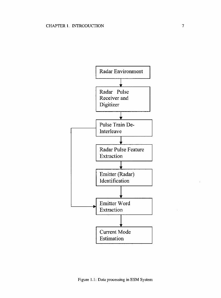
The signal processing in a typical RWR is shown in Figure 1.1. The RWR may
achieve its objective by performing the following three important tasks:
• Pulse Train De-interleaving - The process of de-interleaving refers to
isolating pulse trains associated with a particular radar from a set of over
lapping pulse trains received from the radar within the RWR range of inter
ception. This is the first step to threat recognition in a RWR, as it is difficult
to identify the individual radars without the pulses being de-interleaved. A
significant way to de-interleaving pulse trains is by exploiting their time of
arrival (TOA).
CHAPTER 1. INTRODUCTION 6
• Emitter Identification - The de-interleaved pulse trains are then used to
identify the particular radar emitter that radiated them. This is done by ex
tracting features that are radar-specific such as pulse-repetition frequency
(PPF), pulse width, amplitude, etc., from the pulses. These extracted fea
tures are then compared with the data stored in the ELINT library. Any
matches found will identify the radar that radiated that particular pulse train.
• Modeffhreat Estimation - Once the particular radar is identified, the
threat posed by the radar needs to be estimated as the threat directly depends
on the radar's mode of operation. In the case of radars with hierarchical
signal structure, the mode of operation can be estimated from the words
extracted from the pulse trains.
1.5 Problem Statement
The problem addressed in this thesis is rooted in the concept of radar-target inter
action. This is an important aspect of EW. It involves all the three main divisions
of EW described earlier. There are two different perspectives to this concept.
From the radar's perspective it needs to search, detect, and track the target of
interest. It needs to identify the critical parameters of the target such as its velocity,
direction, etc. Besides these functions, the radar has to perform efficiently in the
presence of any ECM initiated by the target. Therefore from the radar's view the
target represents an uncooperative system that requires to be modeled.
From the target's perspective, say a military aircraft, it has to identify the oper
ational mode of the radar, as the operational mode represents the function that the
radar performs with respect to the target of interest. In this view, the radar itself
CHAPTER 1. INTRODUCTION 7
Radar Environment
~ Radar Pulse Receiver and Digitizer
! Pulse Train De-Interleave
~ Radar Pulse Feature Extraction
~ Emitter (Radar) Identification
Emitter Word Extraction
Current Mode Estimation
Figure 1.1: Data processing in ESM System
CHAPTER 1. INTRODUCTION 8
becomes the target that needs to be tracked. Since the threat level directly de
pends on the operational mode, its knowledge is crucial for the target to estimate
the threat posed by the radar. This is the topic of research addressed in this thesis.
The motivation stems from the fact that, by estimating the operational mode, the
threat can be estimated. This knowledge of threat posed by the radar, helps the
target to initiate measures such as ECM or engage in evasive maneuvers to protect
itself from the radar. This is the task of the RWR.
In order to accomplish this task, the RWR needs to perform the following two
functions:
1. Identify the observed radar.
2. Estimate its operational mode.
In this thesis, we assume the observed radar is identified [15], hence we focus
on estimating the operational mode in an efficient and timely manner. In this
investigation, a recurrent neural network (RNN) trained in a supervised manner,
with dynamic time warping (DTW) algorithm as the post processor is employed to
obtain the minimum distance estimates of the operational modes. These estimates
are smoothed by the application of a grid filter to obtain the posterior estimate of
the radar's current operational mode.
1.6 Organization
This thesis is organized as follows. Chapter 2 describes the essential elements
to the proposed solution, which include a detailed version of the MFR layered
signal architecture and the theory of DTW. Chapter 3 describes the two RNNs
CHAPTER 1. INTRODUCTION 9
employed in the proposed solution, namely, the recurrent multi-layer perceptron
(RMLP) and the echo state network (ESN). This chapter is dedicated to the de
scription of their architecture and training philosophies. Chapter 4 describes in
brief two methodologies that are known in the literature as solutions to the stated
problem. This chapter also states some of their limitations. Chapter 5 describes
the grid filter that is an important component of the proposed solution in a detailed
fashion. Chapter 6 describes the proposed solution with the problem formulation,
methodology, simulation and results. Chapter 7 concludes the thesis with a sum
mary of major contributions and improvements from the proposed methodology
over previous methodologies.
Chapter 2
Essential Elements in the Mode
Estimation of MFR
This chapter introduces some of the essential concepts involved in the mode es
timation of MFR. It describes the layered signal architecture of MFR, which is
proposed to keep the radar signal processing complexity manageable, the idea of
radar mode evolution, and a brief overview on the theory of DTW.
2.1 Hierarchial Signal Structure
As mentioned in Chapter 1, the advancements in electronics and software have
made the MFR a sophisticated military equipment. The pulse structure of MFR
has become more complex as a result of software controlled radar pulse genera
tion. This complex pulse structure along with the capability to perform multiple
tasks makes mode estimation of MFR difficult at the pulse level. Therefore, to
overcome this difficulty and to keep the signal processing complexity manageable
10
CHAPTER 2. ESSENTIAL ELEMENTS IN THE MODE ESTIMATION OF MFR 11
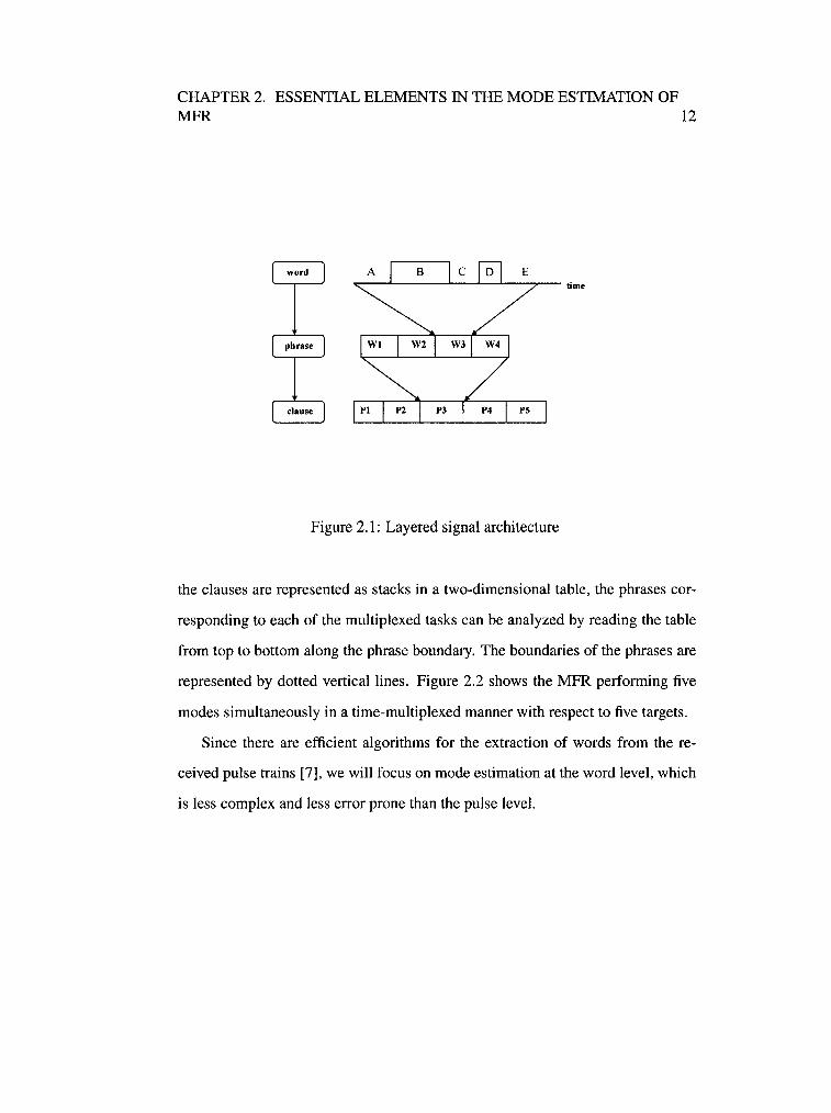
a hierarchial signal structure [6] is proposed as shown in Figure 2.1. Estimation
of the operational mode is obtained through word level processing which is sub
sequent to the pulse level processing.
A word is composed of a specific group of pulses. It is divided into five sec
tions (A-E), of which pulses are transmitted only in section B and section D.
Section B is known as the pulse doppler sequence. The pulse doppler sequence is
unique for each word. It has a set of pulses with a characteristic pulse per interval
(PPI) for each word which makes them unique. Section D is known as the syn-
chronization burst sequence that is common to all the words and sections A,C,E
are known as dead time zones as no pulses are transmitted in these intervals. The
MFR has a total of nine different words (Wl - W9) with similar pulse envelope.
A phrase is made up of a particular combination of four words. Each phrase
represents a mode of operation of MFR but not in a unique way. Therefore, a
particular phrase may represent more than one mode. In the same way several dif
ferent phrases may represent a single mode of operation. For example the phrase
[W6 W6 W6 W6] may represent two modes of operation such as acquisition and
track maintenance. Therefore, the mapping between a mode and a phrase is many
to-many which makes the task of mode estimation for the MFR more complicated.
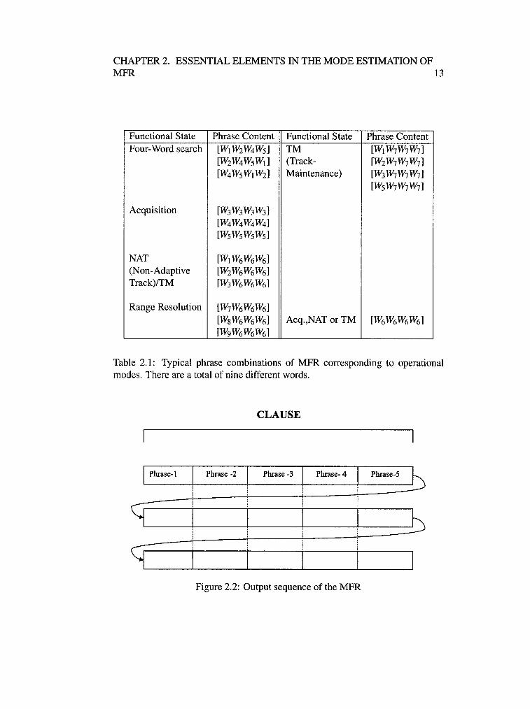
Table 2.1 shows the different operational modes and their corresponding phrase
combinations.
A clause is made up of combination of phrases. The number of phrases in
a clause represents the number of operations performed by the MFR simultane
ously in a time-multiplexed manner. The clauses are concatenated sequentially
one after the other, same as in words and phrases. In that respect the last word
of (n)lh clause is followed by the first word of (n + l)1h clause. However, when
CHAPTER 2. ESSENTIAL ELEMENTS IN THE MODE ESTIMATION OF MFR 12
l word J
[ phrase J
l clause J
Figure 2.1: Layered signal architecture
the clauses are represented as stacks in a two-dimensional table, the phrases cor-
responding to each of the multiplexed tasks can be analyzed by reading the table
from top to bottom along the phrase boundary. The boundaries of the phrases are
represented by dotted vertical lines. Figure 2.2 shows the MFR performing five
modes simultaneously in a time-multiplexed manner with respect to five targets.
Since there are efficient algorithms for the extraction of words from the re
ceived pulse trains [7], we will focus on mode estimation at the word level, which
is less complex and less error prone than the pulse level.
CHAPTER 2. ESSENTIAL ELEMENTS IN THE MODE ESTIMATION OF MFR 13
Functional State Phrase Content Functional State Phrase Content Four-Word search [W1WzW4Ws] TM [W1W7W7W7]
[WzW4WsW1] (Track- [WzW7W7W7] [W4WsW1 Wz] Maintenance) [W3W7W7W7]
[WsW7W7W7]
Acquisition [W3W3W3W3] [W4W4W4W4] [WsWsWsWs]
NAT [W1W6W6W6] (Non-Adaptive [WzW6W6W6] Track)/TM [W3W6W6W6]
Range Resolution [W7W6W6W6] [WsW6W6W6] Acq.,NAT or TM [W6W6W6W6] [W9W6W6W6]
Table 2.1: Typical phrase combinations of MFR corresponding to operational modes. There are a total of nine different words.
CLAUSE
Phrase -2 Phrase -3 Phrase- 4 Phrase-S
Figure 2.2: Output sequence of the MFR
CHAPTER 2. ESSENTIAL ELEMENTS IN THE MODE ESTIMATION OF MFR 14
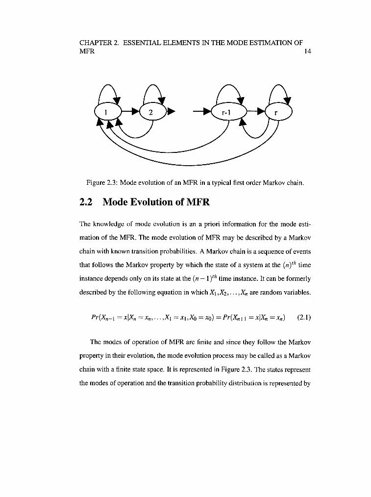
Figure 2.3: Mode evolution of an MFR in a typical first order Markov chain.
2.2 Mode Evolution of MFR
The knowledge of mode evolution is an a priori information for the mode esti
mation of the MFR. The mode evolution of MFR may be described by a Markov
chain with known transition probabilities. A Markov chain is a sequence of events
that follows the Markov property by which the state of a system at the (n) 1h time
instance depends only on its state at the ( n- 1 )lh time instance. It can be formerly
described by the following equation in which x, ,Xz, ... ,Xn are random variables.
Pr(Xn+! = xiXn = Xn, ... ,X, = XJ ,Xo = xo) = Pr(Xn+! = xiXn = Xn) (2.1)
The modes of operation of MFR are finite and since they follow the Markov
property in their evolution, the mode evolution process may be called as a Markov
chain with a finite state space. It is represented in Figure 2.3. The states represent
the modes of operation and the transition probability distribution is represented by
CHAPTER 2. ESSENTIAL ELEMENTS IN THE MODE ESTIMATION OF MFR 15
a matrix with elements given by
Pr(Xn+I = iiXn = j) (2.2)
Therefore, the mode evolution of an MFR is a finite state Markov chain with
known transition probabilities that are invariant in time.
2.3 Dynamic Time Warping (DTW)
DTW is a sequence alignment (template matching) technique widely used in speech
recognition, robotics, pattern recognition, etc. [8]. It is a well known post-processing
tool for neural networks. It is used to measure the similarity between two given
sequences. In DTW, the similarity is estimated as a measure of global distance be
tween the two given sequences. As similarity is inversely proportional to distance,
minimizing the distance signifies maximizing the similarity between the two se
quences. An optimal alignment path is constructed between the two sequences to
measure the global distance between them.
2.3.1 Construction of an Optimal Path
Consider r( i), i = 1 , 2, ... , N and t (j), j = 1, 2, ... , M as the feature vectors rep
resenting the reference and test sequences, respectively. These two vectors need
not be of same length. Now the task is to estimate the similarity between the two
sequences by measuring the global distance between them. Therefore, to accom
plish this, a two-dimensional grid structure is constructed with the elements of the
CHAPTER 2. ESSENTIAL ELEMENTS IN THE MODE ESTIMATION OF MFR 16
5
4.5
4
3.5
g 3
!!l ~ 2.5
~ 2
1.5
2 3 4 5 6 Reference Sequence
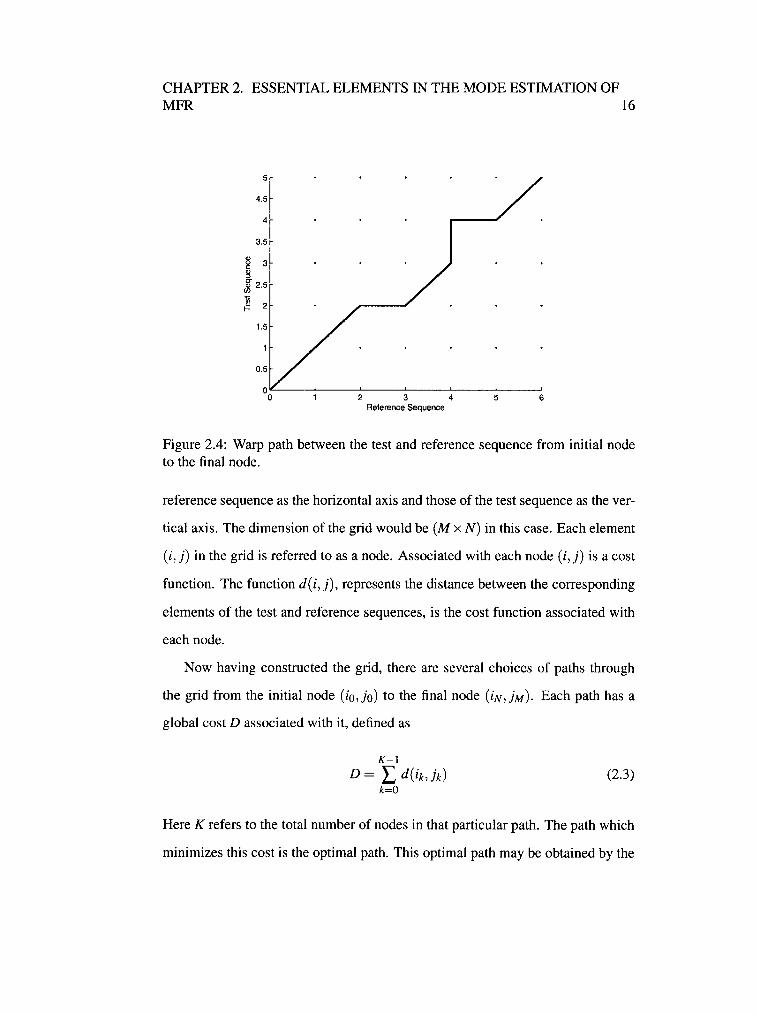
Figure 2.4: Warp path between the test and reference sequence from initial node to the final node.
reference sequence as the horizontal axis and those of the test sequence as the ver
tical axis. The dimension of the grid would be (M x N) in this case. Each element
(i,j) in the grid is referred to as a node. Associated with each node (i,j) is a cost
function. The function d ( i, j), represents the distance between the corresponding
elements of the test and reference sequences, is the cost function associated with
each node.
Now having constructed the grid, there are several choices of paths through
the grid from the initial node (io,jo) to the final node (iN,jM)· Each path has a
global cost D associated with it, defined as
K-1
D = L d(ik, A) (2.3) k=O
Here K refers to the total number of nodes in that particular path. The path which
minimizes this cost is the optimal path. This optimal path may be obtained by the
CHAPTER 2. ESSENTIAL ELEMENTS IN THE MODE ESTIMATION OF MFR 17
principle of dynamic programming (DP). Figure 2.4 shows the warp path between
the test and reference sequence.
2.3.2 Dynamic Programming (DP)
The principle of dynamic programming was first introduced by Bellman [8]. It
states that an optimal path between the initial and final node is the concatenation
of the optimal paths for each of the intermediate nodes that lie between the initial
and final nodes. If (ir. jr) is an intermediate node between the initial node (io, jo)
and final node (iN, jM) and if the optimal path has to pass through it, then by
Bellman's DP the optimal path is given by
( . . ) opt (. . ) (. . ) opt (. . ) (. . ) opt (. . ) lQ,]O --t lN,]M = lO,]O --t lr,]r E9 lr,]r --t lN,]M (2.4)
where ~ refers to the optimal path from one node to another and E9 refers to the
concatenation of these optimal paths. This principle of DP may be applied to find
the optimal path through the grid resulting in minimizing the cost function given
by (2.3). Therefore, the optimal path which minimizes (2.3) is given by
where d(iN, jMiiN-1, jM-1) refers to the cost associated with transition from node
(iN-1 ,jM-1) to node (iN,jM) which is added on to the minimum cost incurred up
to node (iN-1, jM-1) . Step (2.5) is repeated right from the initial node to the final
node. Thus by DP the overall cost is minimized if each of the transitional cost
between the initial node to the final node is minimized. However this is done with
some constraints which determine the direction and scope of node transition.
CHAPTER 2. ESSENTIAL ELEMENTS IN THE MODE ESTIMATION OF MFR 18
i-l,j l,J
/1 i-1,j-1 i,j-1
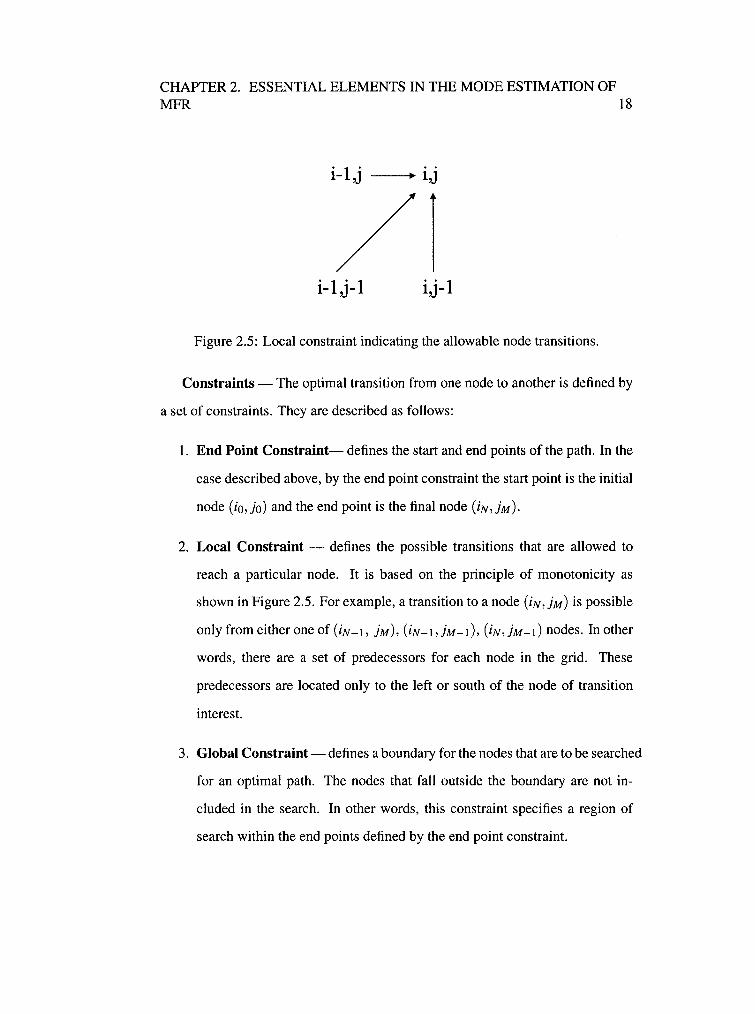
Figure 2.5: Local constraint indicating the allowable node transitions.
Constraints- The optimal transition from one node to another is defined by
a set of constraints. They are described as follows:
1. End Point Constraint- defines the start and end points of the path. In the
case described above, by the end point constraint the start point is the initial
node (io,jo) and the end point is the final node (iN,jM)·
2. Local Constraint - defines the possible transitions that are allowed to
reach a particular node. It is based on the principle of monotonicity as
shown in Figure 2.5. For example, a transition to a node (iN, jM) is possible
only from either one of UN-I, jM). (iN- I ,jM-t), (iN,jM-1) nodes. In other
words, there are a set of predecessors for each node in the grid. These
predecessors are located only to the left or south of the node of transition
interest.
3. Global Constraint- defines a boundary for the nodes that are to be searched
for an optimal path. The nodes that fall outside the boundary are not in
cluded in the search. In other words, this constraint specifies a region of
search within the end points defined by the end point constraint.
Chapter 3
Recurrent Neural Networks (RNNs)
In this chapter, we introduce the concept of recurrent neural networks. We de
scribe in detail two different architectures of RNNs, their training philosophies
and algorithms. The two architectures described are the recurrent multi-layer per
ceptron (RMLP) and the echo state network (ESN).
3.1 Introduction
RNNs are a type of artificial neural networks which are characterized by the use of
feedback. Feedback [ 1 0] is said to exist in a system if the system output influences
the system input in part, by forming a closed loop transmission path from the out
put to the input of the system. RNNs are inspired by the biological neural network
which is recurrent in nature. Due to the presence of feedback RNNs can perform
input-output mapping of a system and hence are dynamically driven networks ca
pable of mimicking dynamic systems with arbitrary precision. RNNs are widely
used in areas such as controls, speech recognition, robotics, telecommunication,
etc., for tasks that include prediction, pattern classification, system identification,
19
CHAPTER 3. RECURRENT NEURAL NETWORKS (RNNS) 20
filtering etc. Though there are different architectures and training algorithms for
RNNs, in this thesis we will focus on two types of RNNs architectures, namely,
the RMLP trained with the extended Kalman filter and the ESN.
3.2 Recurrent Multi-Layer Perceptron (RMLP)
The RMLP [10] [19] is one type of RNN architecture. The RMLP has layers of
neurons between the input and output layers. These layers are called hidden lay
ers. The RMLP must have at least one hidden layer of recurrent neurons. Figure
3.1 illustrates a RMLP with two hidden layers and an output layer. The dynamic
behavior of the RMLP is described by a system of coupled equations [10] as fol
lows.
XJ(n+1) <j>J(XJ(n),u(n))
xu(n+1) = <pu(xu(n),xi(n+1))
Xo(n+ 1) <i>o (x0 (n),xu(n+ 1))
(3.1)
(3.2)
(3.3)
where <j>J(-), <pu(-) and <p0 (-) are the activation functions of the first hidden layer,
second hidden layer, and output layer, respectively.
There are many training algorithms such as back propagation through time
(BPTT), real time recurrent learning (RTRL), extended Kalman filter (EKF), etc.,
to train the RMLP. Each of these algorithms has its own merits. However, in this
thesis we will focus on training the RMLP with the EKF algorithm as it is believed
to give the best results [ 12].
CHAPTER 3. RECURRENT NEURAL NETWORKS (RNNS)
xn(n) Second
x,(n)
Input u(n)
Vector --11!1~ ... .., First
Hidden Layer
Hidden Layer
: L__ __ _J x,(n+ 1) xn(n+ 1) I I : MLP with multiple hidden layers
Output Layer
21
x,(n+l)
1-.--· Output I'!' Vector
L------------------------------------------------
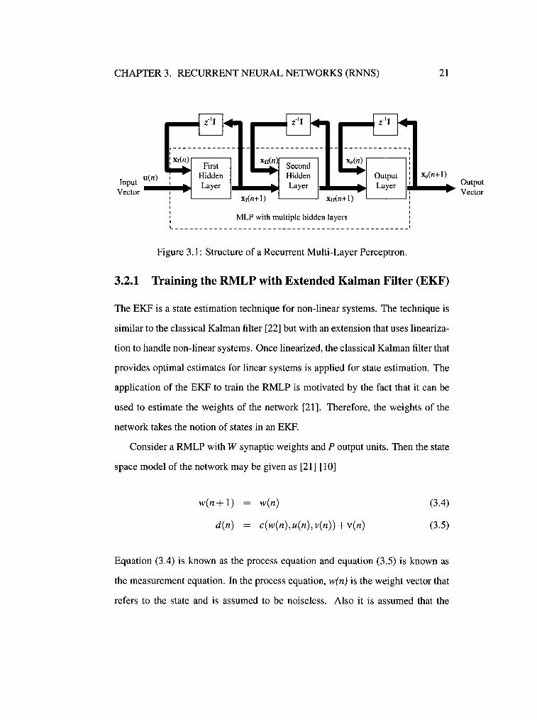
Figure 3.1: Structure of a Recurrent Multi-Layer Perceptron.
3.2.1 Training the RMLP with Extended Kalman Filter (EKF)
The EKF is a state estimation technique for non-linear systems. The technique is
similar to the classical Kalman filter [22] but with an extension that uses lineariza
tion to handle non-linear systems. Once linearized, the classical Kalman filter that
provides optimal estimates for linear systems is applied for state estimation. The
application of the EKF to train the RMLP is motivated by the fact that it can be
used to estimate the weights of the network [21]. Therefore, the weights of the
network takes the notion of states in an EKF.
Consider a RMLP with W synaptic weights and P output units. Then the state
space model of the network may be given as [21] [10]
w(n+ 1)
d(n)
w(n)
c(w(n),u(n), v(n)) +v(n)
(3.4)
(3.5)
Equation (3.4) is known as the process equation and equation (3.5) is known as
the measurement equation. In the process equation, w(n) is the weight vector that
refers to the state and is assumed to be noiseless. Also it is assumed that the
CHAPTER 3. RECURRENT NEURAL NETWORKS (RNNS) 22
network is in an optimum condition with a weight transition matrix being equal to
the identity matrix. In the measurement equation, u(n) and v(n) refers to the input
vector and recurrent node vector, respectively. v(n) denotes the measurement
noise vector which is a zero mean, white noise process with a co-variance defined
by
R(n) = E[v(n)vT (n)J (3.6)
c(.) in (3.5) denotes the entire non-linearity right from the input layer to the output
layer of the RMLP. Therefore, from (3.4) and (3.5) it can be seen that the non-
linearity is associated only with (3.5) hence it is necessary to linearize it before
applying the Kalman filter. The linearized version of (3.5) is given by
d(n) = C(n)w(n) +v(n) (3.7)
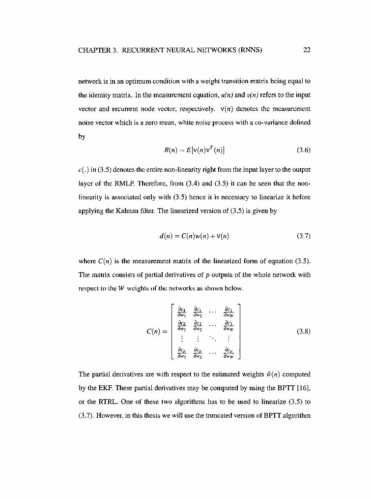
where C(n) is the measurement matrix of the linearized form of equation (3.5).
The matrix consists of partial derivatives of p outputs of the whole network with
respect to the W weights of the networks as shown below.
~ I Pw; 2 ~ w
C(n) = Pw; I
?w; 2 ~ w (3.8)
~ I ~ 2 ~ w
The partial derivatives are with respect to the estimated weights w(n) computed
by the EKF. These partial derivatives may be computed by using the BPTT [16],
or the RTRL. One of these two algorithms has to be used to linearize (3.5) to
(3. 7). However, in this thesis we will use the truncated version of BPTT algorithm
CHAPTER 3. RECURRENT NEURAL NETWORKS (RNNS) 23
as illustrated in [19] to compute the C(n) matrix since it is efficient as well as
computationally affordable. The computation cost for RTRL is O(N4 ). This is
much higher than that of truncated BPTT, which is 0( dN2 ), where N is the number
of recurrent units and d is the truncation depth. Besides computational cost it has
been reported in the literature that best results in training RMLP may be obtained
by using the EKF to estimate the weights of the network with truncated BPTT for
linearization which involves the computation of C( n) [ 12], [ 19]. Therefore with
the computation of C(n) equation (3.5) may be recast in the form of (3.7). Now
the classical Kalman filter may be applied to estimate the weights of the RMLP.
Before deriving the Kalman filter equations, we mention two variations in the
application of EKF, namely,
1. Global EKF
2. Decoupled EKF
In the case of global EKF, the entire linearized measurement matrix C( n) is used as
a whole in the derivation of the Kalman filter. This is computationally expensive
but more accurate. On the other hand, in the case of decoupled EKF the network
synaptic weights may be partitioned into, say, g groups with the i1h group contain
ing }i neurons. Then the partial derivatives of the C(n) measurement matrix have
to be rearranged according to the weights corresponding to each of the individual
neurons in the network in a way that they are grouped as a single block within
C( n). C( n) would then be a concatenation of the partial derivatives corresponding
to each group i, where i = 1, 2, ... , g.
C(n) [C1 (n), · · · ,C8 (n)J (3.9)
CHAPTER 3. RECURRENT NEURAL NETWORKS (RNNS) 24
This decoupled nature of EFK was first introduced in [ 18]. It is computation
ally more efficient than the global EKF with slight compromise in accuracy. The
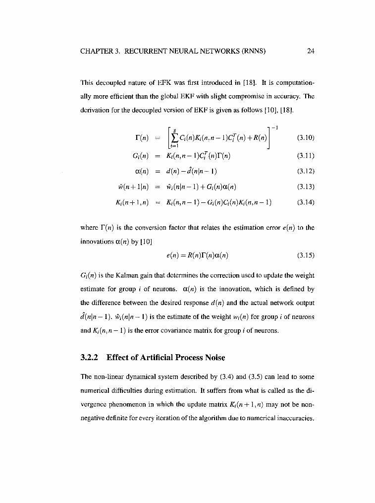
derivation for the decoupled version of EKF is given as follows [10], [18].
r(n) = [,t,c;(n)K;(n,n-I)C{(n)+R(n)]-J (3.10)
Gi(n) Ki(n,n -1)CT (n)r(n) (3.11)
a(n) d(n) -J(nln-1) (3.12)
w(n+1ln) wi(nln- 1) + Gi(n)a(n) (3.13)
Ki(n+ 1,n) = Ki(n,n -1)- Gi(n)q(n)K(n,n- 1) (3.14)
where r(n) is the conversion factor that relates the estimation error e(n) to the
innovations a(n) by [10]
e(n) = R(n)r(n)a(n) (3.15)
Gi(n) is the Kalman gain that determines the correction used to update the weight
estimate for group i of neurons. a(n) is the innovation, which is defined by
the difference between the desired response d ( n) and the actual network output
J(nln-1). wi(nln-1) is the estimate of the weight wi(n) for group i of neurons
and Ki ( n, n- 1) is the error covariance matrix for group i of neurons.
3.2.2 Effect of Artificial Process Noise
The non-linear dynamical system described by (3.4) and (3.5) can lead to some
numerical difficulties during estimation. It suffers from what is called as the di
vergence phenomenon in which the update matrix Ki ( n + 1, n) may not be non
negative definite for every iteration of the algorithm due to numerical inaccuracies.
CHAPTER 3. RECURRENT NEURAL NETWORKS (RNNS) 25
This has to be avoided as Ki ( n + 1, n) represents a covariance matrix which has
to be non-negative definite. This problem can be circumvented by incorporating
artificial process noise in the process (3.4) as follows
w;(n+ 1) = wi(n) + ro;(n) (3.16)
where ro;(n) is the process noise which is assumed to be a zero mean white Gaus
sian noise of diagonal co-variance matrix Qi(n). With the incorporation of roi(n),
(3.14) can be recast into
Ki(n+ 1,n) = Ki(n,n-1)- Gi(n)C;(n)Ki(n,n-1) +Qi(n) (3.17)
Therefore by (3.17), K;(n+ 1 ,n) will remain non-negative definite as long as Qi(n)
is large enough. Apart from overcoming the divergence phenomenon, by the ad
dition of process noise there is less likelihood for the algorithm to be trapped in
local minimum, which therefore results in improved speed of convergence and
accuracy in the solution [ 18]. Hence, because of these benefits we incorporate
artificial process noise in the training of RMLP with EKF algorithm.
3.2.3 Back-Propagation Through Time (BPTT)
The BPTT is a gradient decent algorithm to train a RNN. It is an extension of
the well known back-propagation algorithm which is used to train feed-forward
neural networks. As the back-propagation algorithm cannot be employed directly
to RNN, it is used with an extension and is called back-propagation through time.
The extension here lies in unfolding the RNN in time into a feed-forward net
work. Once this is accomplished, the traditional back-propagation algorithm is
CHAPTER 3. RECURRENT NEURAL NETWORKS (RNNS) 26
employed to compute the weight adjustments. The unfolding of the RNN is done
in time. Some interesting properties relating a RNN with its unfolded counter
part are described in [10]. Once the RNN is unfolded in time into a feed-forward
network the back-propagation algorithm is used to compute the sensitivity of the
network, which is the partial derivatives of the cost function (~) with respect to
the synaptic weights of the network. The cost function is defined by
ni
~totat(no,n!) = 1/2 [, [, e](n) (3.18) n=nojEJ4
where .9l is the set of indices pertaining to those neurons in the network for which
the desired response is specified. no is the start time and n1 is the end time. e](n)
is the error signal at the output of j neuron with respect to some desired response.
However, in minimizing this cost function, the network has to remember informa-
tion right up to the start time no for every iteration. This is computationally too
expensive and is not feasible in real time. Therefore, to overcome this limitation
a truncation depth h is used in which any information older than h time steps will
be ignored. This version is called as the truncated BPTT [20]. The cost function
to be minimized for the truncated BPTT is defined as
~(n) (1/2) [, eJ(n) (3.19) }EJ4
CHAPTER 3. RECURRENT NEURAL NETWORKS (RNNS) 27
By the traditional back-propagation algorithm, the sensitivity of the network is
given by
a~(l) -11-
awji n
11 E OJ(l)xi(l- 1) l=n-h+l
(3.20)
(3.21)
The above equation holds for all j E ..9l and (n- h) < l :::; n. The learning-rate
parameter is represented by 11· The input applied to the i1h synapsis of neuron j at
time (!- 1) is given by Xi (l- 1) and o 1 ( l) is the local gradient defined by
(3.22)
In the case of l = n the local gradient o 1 ( l) is given by
(3.23)
where <p' (.) is the derivative of the activation function u 1 ( l) applied to the neuron
j. In case of (n- h < l < n) the local gradient oj(l) is given by
cp' (u 1(1)) E wk1(l)ok(l + 1) (3.24) kE}l
Equations (3.23), (3.24) are repeated from time n right back to time n- h, and
with the computation of back propagation at time n- h + 1 the adjustment weights
are computed according to (3.21). Thus it can be seen from (3.23) and (3.24) that
the error signals is used only in (3.23) which is the computation at time n. This
indicates that the past records of the desired responses have not been stored which
CHAPTER 3. RECURRENT NEURAL NETWORKS (RNNS) 28
makes the truncated BPTT computationally feasible in real time.
3.3 Echo State Network (ESN)
The echo state network is an RNN recently introduced in [11, 13, 14]. As men
tioned earlier all RNNs are characterized by the use of feedback, inspired by the
biological neural network which is recurrent in nature. RNNs have dynamic mem
ory and are used for black-box modeling of non-linear systems. The ESN differs
from other RNNs in two ways:
1. Architecture- The ESN consists of a large number of recurrent units usu
ally in the order of hundreds (1 00-1 000). These recurrent units form a reser
voir. But, in case of conventional RNN such as the RMLP, recurrent units
are represented in the form of hidden layers and are not large in number.
2. Learning Algorithm - The ESN learning algorithm is supervised in na
ture. In the case of ESN, during training only the output synaptic con
nections are modified, whereas in other RNN learning methods the entire
synaptic connections are altered. The training of ESN is done by linear
regression.
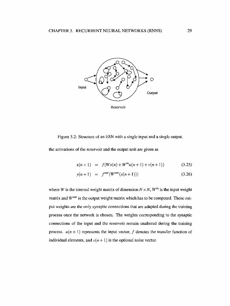
Figure 3.2 shows an ESN with a single input unit, N internal units and a single
output unit. These N internal units are recurrent in nature and thus form the reser
voir of dynamics. The activations of the internal and output units are represented
as x(n) and y(n), respectively. The input is represented by u(n). The updating of
CHAPTER 3. RECURRENT NEURAL NETWORKS (RNNS) 29
0
Reservoir
Figure 3.2: Structure of an ESN with a single input and a single output.
the activations of the reservoir and the output unit are given as
x(n + 1)
y(n + 1)
f(Wx(n) + winu(n + 1) + v(n + 1))
rut (wout (x(n + 1)))
(3.25)
(3.26)
where W is the internal weight matrix of dimension N x N, win is the input weight
matrix and wout is the output weight matrix which has to be computed. These out
put weights are the only synaptic connections that are adapted during the training
process once the network is chosen. The weights corresponding to the synaptic
connections of the input and the reservoir remain unaltered during the training
process. u( n + 1) represents the input vector, f denotes the transfer function of
individual elements, and v( n + 1) is the optional noise vector.
CHAPTER 3. RECURRENT NEURAL NETWORKS (RNNS) 30
3.3.1 Concept of Echo States
A network is an ESN if its dynamic reservoir has echo states. Echo states consti
tute a property that the network exhibits before it is trained. In fact, the echo state
property is related to the properties of the reservoir matrix W. Therefore, a trained
network is an ESN if its untrained version exhibits the echo state property. In this
section, we paraphrase the discussion provided in [12, 14] on the properties and
characterization of echo states. A formal definition of echo states as stated in [14]
is given below.
Definition If an untrained network with weights win, W is driven by teacher input
u(n) from a compact interval U and has network states x(n) from a compact setA,
then the network has echo states if the network state x(n) is uniquely determined
by any left-infinite input u(n- 1), u(n) where n = -2, -1,0.
In an intuitive sense, the echo-state property states that if a network is run
for a very long time from negative infinity (i.e. left-infinite property) then the
current network states can be uniquely determined by the input history. As men
tioned earlier the property of echo states depends on the algebraic properties of
the weight matrix W of the dynamic reservoir. As there is no necessary and suffi
cient algebraic conditions [12] to show that the network has echo states given the
weight matrix (W, win), we resort to a heuristic approach to obtain an echo-state
network. Before describing the heuristics we discuss in proposition (3.3.1) the
sufficient condition for the non-existence of echo states.
Proposition 3.3.1 Consider an untrained network (W, win) with the state update
according to (3.25) and tanh as the transfer function. This network does not have
echo states with respect to the input interval U if the spectral radius of the dynamic
CHAPTER 3. RECURRENT NEURAL NETWORKS (RNNS) 31
reservoir weight matrix W is greater that unity, that is, if l"-maxl > 1. In this, 1"-maxl is the largest absolute value of an eigenvector ofW.
Though there is no sufficient algebraic condition for finding echo-state networks,
in practice it is believed that a network exhibits echo states if Preposition 3.3.1 is
not satisfied. In not satisfying Preposition 3.3.1 the spectral radius 1"-maxl. which
is the largest absolute value of eigenvector of W, is less than unity. Therefore this
heuristic approach [12] as stated in Conjecture 1 is used to design an echo-state
network.
Conjecture 1 Let 8 and E be two small numbers. Then for a dynamic reservoir
of size N a random matrix Wo is created by sampling the weights from a uniform
distribution between [ -1,1]. Then the matrix Wo is normalized to W1 by dividing
Wo by its spectral radius. Scaling W1 to W = (1 - 8)W1 where (1 - 8) is the
spectral radius of W; hence, the network (Win, W) is an echo state network with
probability I -E.
It can be understood from Preposition 3.3.1 and Conjecture 1 that the key to
achieving echo states is by having the spectral radius of the dynamic reservoir less
than unity. It should also be noted that the echo-state property only depends on
the properties of the dynamic reservoir weight matrix W and has nothing to do
with the input weight matrix win. Therefore, the input weight matrix win can be
freely chosen without affecting the echo-state property.
3.3.2 Training an Echo-State Network
Having described the property of echo states along with the heuristic conditions
for an ESN, we present the idea behind training an ESN. First, we discuss the
training principle of an ESN followed by the algorithm employed to train it. A
CHAPTER 3. RECURRENT NEURAL NETWORKS (RNNS) 32
detailed discussion on these topics is presented in [14], [12].
3.3.2.1 Principle
The main difference between an ESN and other RNN structures is that in the case
of ESN only the output synaptic weights are modified during training whereas in
other RNN structures the entire synaptic weights are modified. Therefore the key
aspect of the ESN training lies in the computation of the output weights wout. The
principle employed in the computation of output weights is linear regression. The
training principle is explained as follows.
Consider an ESN, which is to be driven by a set of inputs training data of length
nmax represented by u( n). Then, since the ESN satisfies the echo-state properties
as described in the previous section, after some initial transient period the internal
network states x;(n) of the dynamic reservoir may be represented as
x;(n) ~ e;( ... ,u(n),u(n+ 1)) (3.27)
where e; represents the echo function of the ith unit. The network weight matrix is
assumed to be heterogeneous; therefore, the echo functions will differ from each
other. Let the desired output be denoted by d ( n). Then, the network output is
given by
(3.28)
where wjut represents the ith output connection which needs to be computed. The
rut is a tanh function which is invertible. Hence, (3.28) may be rewritten as
N uout)-ly(n) = E wfutx;(n)
i=l
(3.29)
CHAPTER 3. RECURRENT NEURAL NETWORKS (RNNS) 33
The echo functions as in (3.27) are substituted for Xi(n) in (3.29) which gives
N (fout)-Iy(n) = L wjutei( ... ,u(n),u(n+ 1))
i=I (3.30)
Now the output weights wout which constitute the key ingredient in the training of
an ESN are computed by minimizing the training error in the mean square error
(MSE) sense. The training error is given by
Substituting (3.30) in (3.31), the error is obtained as
N
trrain(n) = (!out)-! d(n)- [. wjut ei(. .. , u(n), u(n + 1)) i=I
Therefore, the MSE, which is to be minimized to obtain wout, is given as
1 nmax
MSErrain = (n _ n . ) L c?rain(n) max mm i=nmin
Now, (3.33) can be written as
(3.31)
(3.32)
(3.33)
(3.34)
where nmin refers to the length of the initial transient that is dismissed and not
used in the computation of the output weight. Since the minimization of (3.33)
is a linear regression task, the training of the ESN which mainly involves the
computation of the output weight wout matrix is by linear regression. If rut = 1
CHAPTER 3. RECURRENT NEURAL NETWORKS (RNNS) 34
as in the case of linear units then (3.34) may be written as
( )
2 1 nmax N
MSEtrain = (n -n . ) L d(n)- L wju1xi(n)
max mm i=nmin i= I (3.35)
3.3.2.2 Algorithm
The training algorithm for an ESN may be described in four stages:
1. Procure an ESN
2. Network state updating
3. Computation of output weights
4. Testing
The first three stages constitute the training phase, and the last stage is the testing
phase.
Procure an ESN - An ESN is one which satisfies the echo-state properties
described earlier. Therefore, to accomplish this we follow the heuristic approach
as discussed in Preposition 3.3.1 and Conjecture 1. The following heuristics guar
antees an ESN.
• The network weight matrix Wo, is a sparse matrix generated randomly from
a uniform distribution [ -1, I]. It is then normalized to W1 with the absolute
value of its spectral radius.
• The Network weight matrix W which has the echo state property is then
obtained as W = aW1 where a < 1 is the spectral radius of W.
CHAPTER 3. RECURRENT NEURAL NETWORKS (RNNS) 35
• The input weights win are randomly generated. Now the untrained network
win, W is an ESN.
• The size of the weight matrix W is always between T /10 and T /2, depend
ing on the complexity of the task. T is the length of the training data.
• The parameter a is of crucial importance for the successful training of an
ESN. Since the spectral radius of the reservoir weight matrix is connected
to the intrinsic timescale of the dynamics of the reservoir state, a diligent
choice of a would improve the probability of successful training. Typical
range of a lies between (0.78 - 0.98).
Network State Updating - Once the ESN is setup, it can be trained by
presenting the input training sequence u(n). The state update is done as follows:
• The initial network state is set to zero, x(O) = 0. Then the network is trained
by presenting the input training data u(n) and the network state update is
performed by
x(n+ I)= f(Wx(n) + winu(n+ 1) +v(n+ 1)) (3.36)
• For each time n, after an initial transient, the network states x(n) are col
lected as a row in a state collecting matrix M and the sigmoid-inverted de
sired output tanh- 1d(n) is collected as a row in a output collecting matrix
T.
Computation of Output Weights - This is the most important part of the
training algorithm since in the case of ESN only the output weights are adapted.
In the previous section, it was shown that the computation of wout is a linear
CHAPTER 3. RECURRENT NEURAL NETWORKS (RNNS) 36
regression task. This can be achieved by multiplying the pseudo-inverse of M
which stores the collected network states with T which stores the collected desired
output:
(3.37)
Thus the output weight wout is obtained as the transpose of (woury.
Testing- The network is trained once the computation of wout is done. The
computed wout is then written in the output weights and the network (W, win, wout)
is ready to be tested. The trained network is tested by presenting a novel input se
quence u(n) and employing (3.25) and (3.26) as the update equations.
Chapter 4
Known Techniques for Mode
Estimation
In this chapter, we briefly describe two stochastic modeling techniques which are
known in the literature as solutions to the mode estimation problem of MFR. The
first technique is based on syntactic modeling, which employs stochastic gram
mar. Here a hidden Markov model (HMM) filter is used to estimate the mode of
operation of the MFR. Some limitations of this technique were overcome by the
second method, the multi-model stochastic approach which is based on observ
able operator model (OOM). This approach exploits the principle of maximum
likelihood to estimate the mode of operation of MFR. This technique also has
some limitations of its own, which leads to the development of a more efficient
model which is described in Chapter 6. The two stochastic modeling techniques,
namely, syntactic modeling and OOM-based modeling are described briefly in the
following sections.
37
CHAPTER 4. KNOWN TECHNIQUES FOR MODE ESTIMATION 38
4.1 Syntactic Modeling
The syntactic modeling technique [6] is based on formal language processing us
ing grammars for modeling. Grammar is a well-known modeling tool in formal
language processing. They help in efficient application of formal language. There
are two types of grammar, namely, deterministic grammar and stochastic gram
mar. In MFR modeling, the radar is assumed to communicate in a formal lan
guage, and stochastic grammar is used to model the same.
4.1.1 Formal Language
A formal language L may be defined as follows.
Definition If A is a set of alphabets of some finite length defined by A =a, b, e, ...
then the language L defined over A is the set of finite length strings formed by
concatenating the alphabets of A.
Two kinds of sets can be formed by concatenating the alphabets in A
a, b, e, ab, be, ea, aa, bb ...
E, a, b, e, ab, be, ea, aa, bb ...
(4.1)
(4.2)
where A+ refers to positive closure of A and A* refers to kleene closure of A as it
contains E. E is an empty string which contains no alphabets. Formal language by
itself has limited application. A better way to employ formal language is by the
use of grammar.
CHAPTER 4. KNOWN TECHNIQUES FOR MODE ESTIMATION 39
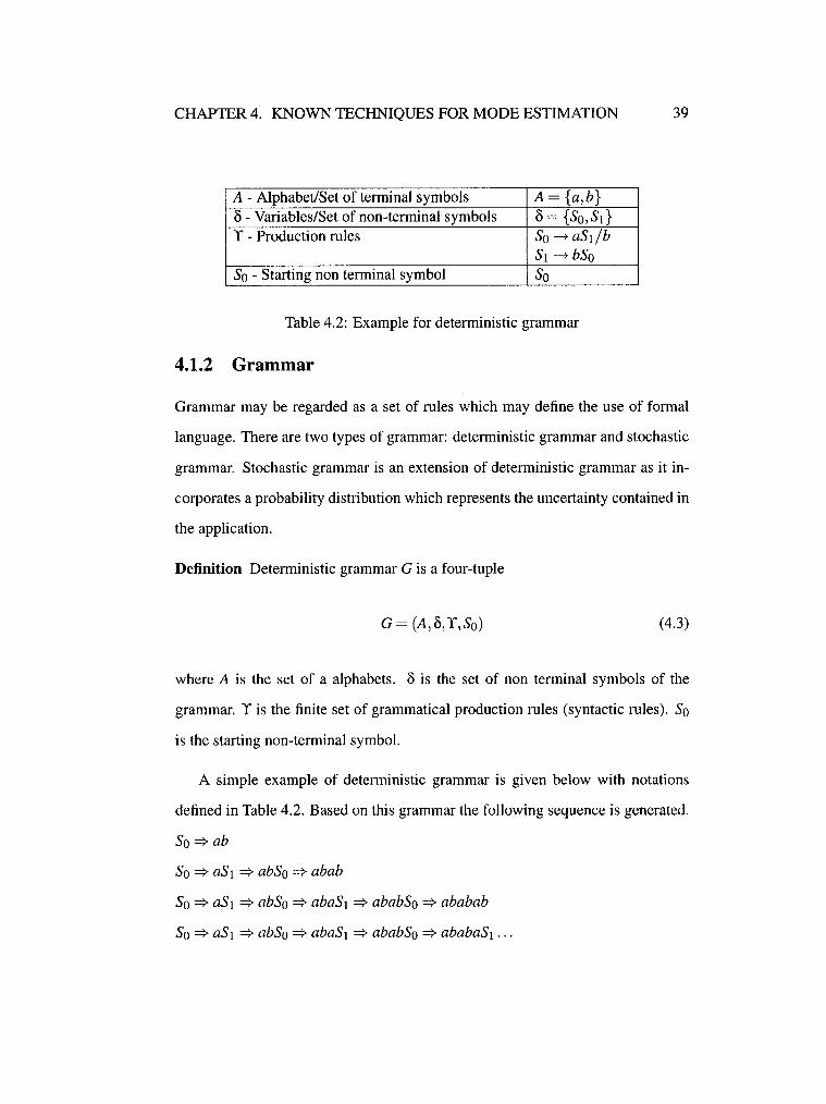
A - Alphabet/Set of terminal symbols A={a,b} o -Variables/Set of non-terminal symbols o = {So,S!} Y - Production rules So-+ aSJ/b
S1-+ bSo So - Starting non terminal symbol So
Table 4.2: Example for deterministic grammar
4.1.2 Grammar
Grammar may be regarded as a set of rules which may define the use of formal
language. There are two types of grammar: deterministic grammar and stochastic
grammar. Stochastic grammar is an extension of deterministic grammar as it in-
corporates a probability distribution which represents the uncertainty contained in
the application.
Definition Deterministic grammar G is a four-tuple
G= (A,o,Y,So) (4.3)
where A is the set of a alphabets. o is the set of non terminal symbols of the
grammar. Y is the finite set of grammatical production rules (syntactic rules). So
is the starting non-terminal symbol.
A simple example of deterministic grammar is given below with notations
defined in Table 4.2. Based on this grammar the following sequence is generated.
So=? ab
So =? aS 1 =? abSo =? abab
So=? aS1 =? abSo =? abaS1 =? ababSo =? ababab
So=? aS1 =? abSo =? abaS1 =? ababSo =? ababaS1 ...
CHAPTER 4. KNOWN TECHNIQUES FOR MODE ESTIMATION 40
The above described production rule is known as regular grammar. By ex
ploiting the properties of production rules four classes of grammar are defined
in a hierarchial fashion in [30]. These four classes of grammar listed below are
known in the literature as Chomsky hierarchy of transformational grammar.
1. Regular Grammar
2. Context-Free Grammar
3. Context-Sensitive Grammar
4. Unrestricted Grammar
The syntactic modeling ofMRF is rooted in the transformation of context-free
grammar. Here, the production rule is defined in the form of S ---+ j), in which the
left hand side of the production rule must contain only one non-terminal symbol
whereas the right hand side can be any string. Many practical applications con
tain some amounts of uncertainty. The uncertainty element may be represented in
the form of probabilistic distribution. To illustrate uncertainty, we take the radar
signal as an example. Radar signals are typically observed in the noisy environ
ment which may cause sparseness in observation. This leads to an extension of
deterministic grammar, which is known as stochastic grammar.
Definition Stochastic grammar Gs is a five tuple
Gs = (A,cS,Y,Ps,So) (4.4)
where Ps is the probability distribution over the set of production rules Y. Rest
of the notations have the same meanings as defined earlier. A more detained
description of grammar and its various forms may be found in [24].
CHAPTER 4. KNOWN TECHNIQUES FOR MODE ESTIMATION 41
4.1.3 Finite State Automata (FSA)
Definition A FSA is a five-tuple
A (Q,I,B,So,F) (4.5)
where Q is the set of states of the FSA. I is the set of input symbols of the FSA. 8
is the transition function of the FSA. So is the initial state of FSA. F is the set of
final (accepting) states of the FSA (F c Q).
It is shown that FSA is equivalent to regular languages, regular grammars and
regular expressions [6]. Chomsky has shown that finite state language can be
generated from CFG if the non-self embedding property is satisfied.
4.1.4 Hidden Markov Model (HMM)
In the syntactic modeling approach mode estimation of MFR is solved by employ
ing a HMM filter. A HMM estimates the underlying state of a model with the help
of noisy observations.
Definition A HMM is a three-tuple defined by
{A,B,<Oo} (4.6)
where A is the Markov matrix/state transition matrix. B is the emission probability
matrix. roo is the initial state probability vector.
The transition and emission probabilities are generated by the syntactic con
cepts described in the previous section with probabilities as defined in stochastic
CHAPTER 4. KNOWN TECHNIQUES FOR MODE ESTIMATION 42
grammar. Finally, a HHM filter is used to estimate the mode of the radar in a
recursive manner. For a detailed description of HMM and the mode estimation
methodology using HMM readers may refer to [6], [23] respectively.
4.1.5 Limitations
The following are the known limitations of this model as described in [3].
• The modeling of MFR is based on the context-free grammar, which needs
to satisfy the non-self embedding property in order to generate FSA. There
fore, there is no guarantee that all radar grammars would pass this test.
• If a realistic radar is considered, the number of states in the word level
HMM is quite large. Consequently, it becomes more expensive in terms of
computational time and memory resource.
• Clustering of the HMM states needs to be performed to estimate the mode
of the radar at any given time. This may lead to lack of accuracy in the radar
mode estimate
• HMM filtering algorithm is valid for a stationary process. However, an
input for the HMM filter is collected from the radar environment which is
non-stationary.
• Finally, from the results presented in [6], there exists frequent mode jumps
in the HMM estimate, which leads to unreliability and lack of accuracy.
Some of these limitations were overcome by the OOM model described in the
following section.
CHAPTER 4. KNOWN TECHNIQUES FOR MODE ESTIMATION 43
4.2 Observable Operator Model (OOM) based Mod
eling
OOM is a stochastic modeling tool developed in [25]. It is comparable to the
well-known HMM with respect to modeling dynamic systems and stochastic time
series. One application example of OOM is to learn the underlying probability
distribution of an unknown system based on its training data. In this section,
we describe in brief the essence of the OOM and the multi-model approach for
mode estimation of MFR. For a detailed description of OOM, readers may refer
to [25] [26].
Definition An m-dimensional OOM is a three tuple, A= (9\m, ( 'ta)aEE, Wo), where
roo E 9\m and 'ta : 9\m ---. 9\m are linear maps represented by matrices, satisfying
1. 1 Wo = I, where 1 = (I , ... , I) E 9\m
2. 11 = LaEE 'ta has column sum equal to 1, where I: is the alphabet.
where m is the dimension of the vector space spanned by the prediction function
and 9\m is the domain of the operators. 'ta is the operator indexed over the output
symbol "a" of the stochastic process. roo is the initial state vector and 1roo refers
to the component sum of WQ.
4.2.1 Why Observable Operators
Consider a system with state space I: consisting of two states (A,B). Then the tran
sition from one state to another is known as the trajectory of the system. This is de
fined by the application of a single operator T. Therefore, the trajectory would be
CHAPTER 4. KNOWN TECHNIQUES FOR MODE ESTIMATION 44
a concatenation of states .... ,A,B,A,A, .... visited by the system. In OOM theory,
this trajectory is viewed in a complimentary fashion. The states are represented as
operators ( TA, TB). Suppose one of these two operators has to be chosen stochasti
cally, then the trajectory refers to the transition from one operator to another. The
trajectory is formed by concatenating the operators TA (T8(TA (TA) ... ) ) .... since the
observable themselves are the operators the model is named as the observable
operator model [26].
4.2.2 Multi-Model Approach
In this section, we briefly describe the algorithm employed to estimate the oper
ational mode of MFR. This multi-model approach [3] makes use of pre-trained
OOMs. The radar is assumed to operate within a finite number of modes which
are known. Then for each mode of operation an OOM is built. The number of
OOMs built is proportional to the number of modes of the radar. These OOMs
may be called as mode specific OOMs. Each mode specific OOM is trained with
word sequences corresponding to that particular mode of operation. The training
is done by the OOM learning principle of Efficiency Sharping. This principle of
training OOMs is believed to overcome some known limitations of the expectation
maximization algorithm which is used to train HMMs [27].
The mode estimation of MFR is done by computing the likelihood of the in
coming words with each of the mode specific OOM model. This is done in a
frame-by-frame manner. The likelihood function (n1(k)) for a frame at time (k)
CHAPTER 4. KNOWN TECHNIQUES FOR MODE ESTIMATION 45
is given as
P( wordsimodel)
P(z(k) IMj(k))
(4.7)
(4.8)
(4.9)
where nj(k) represents the likelihood function for a particular frame at time k.
z(k) refers to the frame of words at time k. Mj refers to the finite number of
modes of MFR with j = 1, ... , r. 't and roo refer to the operator and initial state
vector of the OOM model associated with mode j respectively. Finally, the mode
at time k is obtained by maximizing the likelihood function Q.j(k). Therefore, the
maximum likelihood estimate given by
M(k) = argmaxnj(k) MJ
(4.10)
The maximum likelihood estimate makes frequent jumps from one mode to an
other because of the absence of prior information. This makes the maximum like
lihood estimate unreliable. This is overcome by the use of a grid filter, described
in the next Chapter. The grid filter incorporates prior knowledge about the radar
in the form of transition probabilities. The likelihood estimates of OOM are fed
to the grid filter along with the mode transitional probabilities . The output of the
grid filter is maximized at each time k to obtain the filtered estimate. The filtered
estimate is known as the maximum a posteriori estimate which is free of mode
jumps. A more elaborate version of this approach may be found in [3].
CHAPTER 4. KNOWN TECHNIQUES FOR MODE ESTIMATION 46
4.2.3 Limitations
Though the multi-model OOM approach is said to have overcome some of the
limitations [3] of the syntactic modeling technique, it has some limitations of its
own. Following are the limitations associated with this multi-model approach.
• The OOM modeling is a multi-model approach, which involves building
individual OOM models for each mode of operation. The task of building a
model for each mode of operation could be impractical especially when the
number of operational modes is high.
• The words from the word extractor module are usually corrupted due to
the unfavorable effects of the environment. The word corruption tolerance
supported by the multi-model OOM approach is much less than 10%. This
places a high demand on the performance of the word extractor module.
Therefore, a model with improved word corruption tolerance is needed.
• The OOM multi-model approach fails to detect the mode of operation when
the radar dwell time for that particular mode is less than eight phrases [3].
• The latency associated with the MAP estimate is large.
The above limitations of the multi-model approach lead to the design of a
more reliable and robust technique for the mode estimation of MFR. This novel
estimation technique, described in Chapter 6, overcomes the above mentioned
limitations in an efficient manner.
Chapter 5
Introduction to Grid Filters
This chapter offers a brief description of grid filters. The grid filter is a recursive
state estimation technique to estimate the state of dynamic systems. Systems in
which the state changes over time are called dynamic systems. The grid filter is
a Bayesian filter. A recursive Bayesian filter computes the posterior pdf of the
state of the system in a recursive fashion by incorporating prior knowledge of the
system. In the following sections, we introduce the concept of Bayesian tracking
and the algorithm of grid filter.
5.1 Bayesian Approach for State Estimation
In order to analyze and make inference about a dynamic system, two models are
required namely,
1. The system model which describes the evolution of the state with time.
2. The measurement model which relates the noisy measurement to the state.
47
CHAPTER 5. INTRODUCTION TO GRID FILTERS 48
These two models in general may be available in probabilistic form. This prob
abilistic state space model and the requirement for the updating of information
on receipt of new measurement are ideally suited for the Bayesian approach [ 17].
The main concept of the Bayesian approach lies in the construction of the posterior
probability density function (pdf) of the state with all the available information,
including the measurements received up to the current time instant. Since the pdf
is constructed with all the available statistical information, it is possible to obtain
the optimal estimate of the state from the pdf. For these reasons, such a pdf may
be said to be a complete solution to the state estimation problem of a dynamic
system.
The state of the dynamic system has to be estimated at each time instant. This
calls for a recursive type of filtering approach. In the case of recursive filtering,
the data are processed in a sequential manner when they are received, so there is
no need to store the past history of data. This is realized in two steps, namely, the
prediction step and the update step. The prediction step is used to predict the state
of the system forward from one measurement time to another by employing the
system model. Since the state is usually subject to some random noise the predic
tion may not be accurate, hence an update step is used to modify the predicted pdf.
This update step uses the latest measurement and is achieved by Bayes' theorem,
hence the name "Bayesian" approach.
5.2 Bayesian Tracking
Having described the concept of the Bayesian approach for a dynamic state es
timation problem, we will now see how the prediction and update equations are
CHAPTER 5. INTRODUCTION TO GRID FILTERS 49
developed [ 17]. In order to describe a dynamic system, consider the following
two models.
1. The system model describing the evolution of the state sequence { XkJ k E N}
of a system, is given by
(5.1)
where fk : 9\nx x 9\nv -----t 9\nx is a non-linear function of Xk-1 and vk-1·
{ Vk-1, k E N} is an independent and identically distributed (i.i.d) process
noise sequence. nx & nv are dimensions of state and process noise vectors,
respectively.
2. The measurement model, from which the state of the system is to be esti
mated recursively, is given by.
Zk (5.2)
where hk : 9\nx x 9\nn -----t 9\ny is possibly a non-linear function. { nkl k E
N} is an i.i.d measurement noise sequence. ny & nn are dimensions of
measurement and measurement noise vectors respectively.
The objective of the filter is to estimate the state xk of the system, given all
the available information (measurement) Zk = {zili = 1, ... ,k}. From a Bayesian
perspective, this requires the calculation of the posterior density function p(xkiZk)·
It is assumed that the initial state pdf p(xolzo) = p(xo) is given. Then p(xkiZk) can
be sequentially obtained in two stages: the predict stage and the update stage.
CHAPTER 5. INTRODUCTION TO GRID FILTERS 50
The predict stage uses the system model to predict the state of the system at
one time step ahead using past measurements. Assuming that the required pdf
p(xk-IiZk-I) at time (k- 1) is available, prediction is given by the Chapman
Kolmogorov equation as follows:
where p(xkiXk-d refers to the state transition of the system.
The update stage uses the current measurement Zk to modify the state predic
tion at time p(xkiZk-J), and this is carried out via Bayes' rule:
p(zkixk)p(xkiZk-I)
P(YkiZk)
where P(YkiZk) = J p(zkixk)p(xkiZk-I)dxk is the normalization constant.
(5.4)
The current state estimate p(xkizk) is used as the past estimate in the prediction
equation (5.3) for the next time instant (k + 1 ), forming a recursive propagation.
This recursive propagation of the posterior probability density function is actually
a conceptual solution and cannot be determined analytically. The analytical so
lution does exist but with certain restrictions. One such solution to this Bayesian
recursive filtering is the grid filter, which is described in the next section.
5.3 Grid Filter Algorithm
The grid filter provides optimum solution to the Bayesian recursive equations (5.3)
and (5.4) if the following two conditions hold:
• State space model is discrete
CHAPTER 5. INTRODUCTION TO GRID FILTERS 51
• Number of states in the state space is finite
Suppose the state space at time k- 1 consists of discrete states xL 1, i = 1, ... , r. For each state x;, let the conditional probability of the state given measurements
up to time step (k- 1 ), be denoted by
CJi k-llk-1 Pr(.xk-1 = xL Ilzk-1)
Then the posterior pdf of the state at time k- 1 is given by
r
EroLIIk-I8(.xk-I-.xLI) i=!
(5.5)
(5.6)
where 8(.) is the Dirac delta. Substitution of (5.6) in (5.3) and (5.4) yields the
prediction and update equation at time step (k), respectively, as follows:
where
r
p(xkiZk-!) L ro~lk-!8(xk- xk) i=!
r
p(xkiZk) E ro~lko(xk - xD i=!
r
L roL Ilk- I P(xkl.xi-1) j=!
(5.7)
(5.8)
(5.9)
(5.10)
The above equations assume that p(.xkl.x{_1) and p(zklxk) are known but they
do not constrain the particular form of these discrete densities. This solution of
grid filter is optimal only if the above mentioned assumptions hold.
Chapter 6
RNN-DTW hybrid for Mode
Estimation of MFR
In this chapter, we formulate the mode-estimation problem and describe our novel
methodology to track the operational mode of MFR. This methodology, the RNN
DTW hybrid, employs a RNN trained in a supervised manner with the DTW algo
rithm as the post processor [28] to estimate the operational mode. The approach is
tested for an EW scenario via simulation by employing a hypothetical MFR. The
simulation is performed with two types of RNN for comparison, namely the ESN
and the RMLP which were described in Chapter 3.
6.1 Problem Formulation
For the RWR to estimate the operational mode, it must first classify the observed
radar. In the context of this work, we assume the radar is already classified based
on the characteristics of the received signal [15]. Therefore, having classified the
52
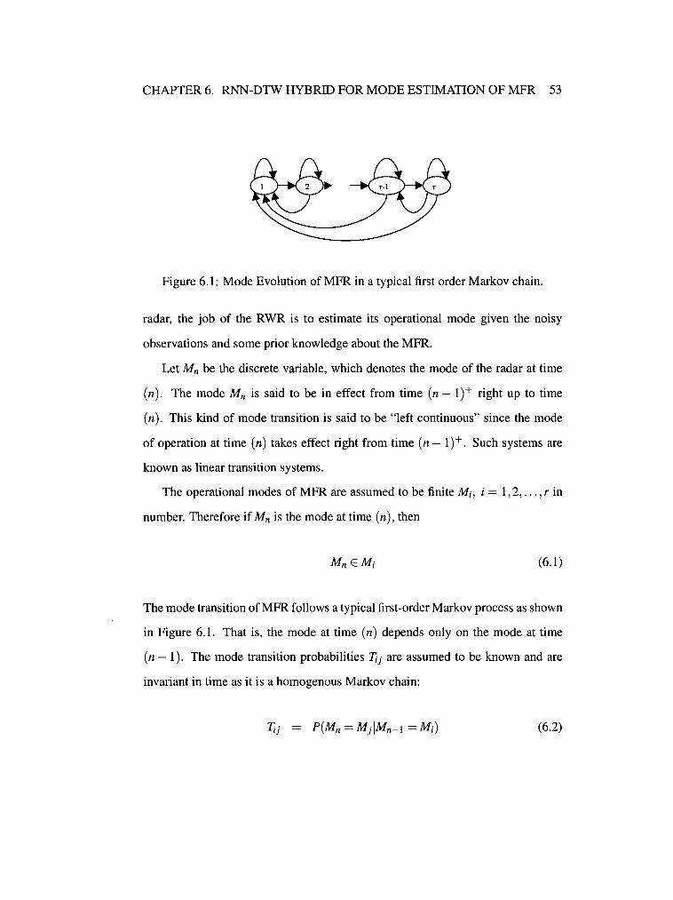
CHAPTER 6. RNN-DTW HYBRID FOR MODE ESTIMATION OF MFR 53
Figure 6.1: Mode Evolution of MFR in a typical first order Markov chain.
radar, the job of the RWR is to estimate its operational mode given the noisy
observations and some prior knowledge about the MFR.
Let Mn be the discrete variable, which denotes the mode of the radar at time
(n). The mode Mn is said to be in effect from time (n -1)+ right up to time
( n). This kind of mode transition is said to be "left continuous" since the mode
of operation at time (n) takes effect right from time (n -1)+. Such systems are
known as linear transition systems.
The operational modes of MFR are assumed to be finite M;, i = 1, 2, ... , r in
number. Therefore if Mn is the mode at time (n), then
(6.1)
The mode transition of MFR follows a typical first-order Markov process as shown
in Figure 6.1. That is, the mode at time (n) depends only on the mode at time
(n- 1 ). The mode transition probabilities Tij are assumed to be known and are
invariant in time as it is a homogenous Markov chain:
(6.2)
CHAPTER 6. RNN-DTW HYBRID FOR MODE ESTIMATION OF MFR 54
6.2 Methodology
The operational mode of MFR is estimated sequentially in two stages in the fol
lowing order:
1. Minimum Distance Estimate
2. Maximum a-Posteriori Estimate
The computation of the minimum distance estimate is the most crucial part
of the algorithm. A RNN-DTW hybrid is used for this purpose. The maximum a
posteriori estimate, which is the second stage of the algorithm, is used to refine the
minimum distance estimate. A grid filter is applied for this step. The following
subsection describes the two stages in detail.
6.2.1 Minimum Distance Estimate
The pulses received from the radar are de-interleaved and given to a word extractor
module. The words from the word extractor are fed to a trained RNN in a sliding
window fashion. The words from the word extractor may usually contain erro
neous words as a result of various corruption effects. A RNN is setup and trained
to learn the underlying word generation mechanism of the MFR. The training is
carried out in a supervised manner with the known sequence of words available
for each mode of operation. In the simulation, we have tested the algorithm for
two types ofRNN: the ESN and the RMLP trained with the EKF algorithm. These
two networks and their respective training principles were described in Chapter 3.
The output of RNN needs to be processed to obtain the modes. The DTW
is used as a post processor. The stream of words from the RNN are fed into
CHAPTER 6. RNN-DTW HYBRID FOR MODE ESTIMATION OF MFR 55
a windowing module. Here the word sequences are split into non-overlapping
windows of fixed length. The choice of the window size is a design parameter.
Mode estimation is carried out in a sequential window fashion with one window
at a time. This offers the following advantages:
• Mode estimation by a sequential window fashion helps detect the radar
mode transition in a precise manner.
• Sequential window processing helps keep the error growth under control in
the case of a mismatched mode estimate at any given time.
Each window from the windowing module is considered as a test sequence
Tn (at time n) and is compared with a finite set of reference sequences Ri, i =
1, 2, ... , r pertaining to each mode. Each reference sequence is a feature vee-
tor describing a particular operational mode. It is the result of concatenation of
phrases which correspond to that particular mode of operation. The test sequence
and reference sequences can be of varying lengths. The choice of their length
is a design parameter. However, it is worthy to note that smaller size sequences
increase the probability of timely mode estimation and timely detection of mode
transition.
The comparison criterion is the distance. The DTW technique described in
Chapter 2 estimates the distance of each reference sequence from the test se-
quence:
. [Ef=I WJ] Di(Tn,Ri) = mm K i (6.3)
where w1 refers to the optimal warp path from the initial node to the final node of
the grid constructed between the test sequence and each of the reference sequence
as described in Chapter 2. This optimal warping minimizes the global distance
CHAPTER 6. RNN-DTW HYBRID FOR MODE ESTIMATION OF MFR 56
between the two sequences. Therefore, the minimum distance estimate (M':/0 ),
which is the mode at time (n), is obtained as
(6.4)
6.2.2 Maximum a-Posteriori Estimate
It can be seen from the simulation results that the minimum distance estimate
makes occasional mode jumps. This is due to the lack of prior knowledge of the
radar. A logical method to overcome this occasional mode jump is by incorporat
ing prior knowledge about the radar into the mode estimation algorithm. This is
achieved by applying a grid filter, described in the previous chapter, to the com
puted minimum distance estimates. The grid filter, which actually smooths the
minimum distance estimate, exploits the known transitional probabilities (TiJ) of
the radar, which is a prior knowledge. The solution of the grid filter is optimal
under the assumption that the state space is discrete and finite [ 17]. The choice
of grid filter is motivated by the fact that in our problem the operational mode
represents the state of the filter and thus satisfies the assumption. The governing
equations of the grid filter modeled in the mode estimation frame-work are given
as
(6.5)
(6.6)
CHAPTER 6. RNN-DTW HYBRID FOR MODE ESTIMATION OF MFR 57
where 'FiJ is the known mode transition probability, which is used as the prior
knowledge of the radar. ro~_ 11n_ 1 is the initial mode probability for each mode
of operation. ro~ln- 1 is obtained from the first step of the grid filter, which is
(6.5). Di(Tn,Ri) is the minimum distance estimate obtained from the first step
of the mode estimation algorithm. Its inversion in the normalized form gives the
probabilistic version of the MMD estimate.
The grid filter provides the posterior estimate of the radar's operational mode.
Therefore, the current mode Mn of the radar is obtained as a maximum a-posteriori
estimate by maximizing the posterior mode probability and is given by
(6.7)
Figure 6.2 illustrates the entire mode estimation methodology. As mentioned ear
lier, this novel approach is tested via simulation for two different RNN networks.
The simulation and results are presented in the next section.
6.3 Simulation
In this section, we explain the computer simulations conducted to test our method
ology in the following hypothetical EW scenario. Imagine a MFR stationed on
the ground. There are five modes of operation, namely, search, acquisition, non-
adaptive track, range resolution and track maintenance that the MFR can perform.
Now assume an aircraft fitted with a RWR is approaching the MFR air space. As
the aircraft enters the radar detection territory, the radar will begin to engage the
aircraft and evolve from one mode to another in a Markovian process as described
earlier in Chapter 2. Now it is the job of the RWR to estimate and track the mode
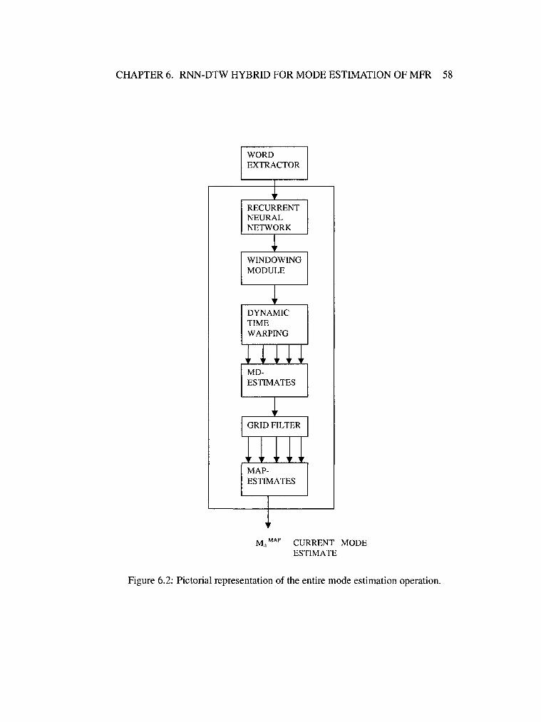
CHAPTER 6. RNN-DTW HYBRID FOR MODE ESTIMATION OF MFR 58
WORD EXTRACTOR
+ RECURRENT NEURAL NETWORK
~ WINDOWING MODULE
~ DYNAMIC TIME WARPING
~ ~ ~ ~ ~ MD-ESTIMATES
~ GRID FILTER
11111 MAP-ESTIMATES
Mn MAP CURRENT MODE ESTIMATE
Figure 6.2: Pictorial representation of the entire mode estimation operation.
CHAPTER 6. RNN-DTW HYBRID FOR MODE ESTIMATION OF MFR 59
evolution of the MFR as this information is vital for the aircraft to estimate the
threat posed by the radar.
A hypothetical radar was setup, which depicts the above mentioned scenario.
For each mode of operation a corresponding phrase from Table 2.1 is assigned.
The phrase selection is done randomly by generating random numbers from a
uniform distribution of (0 to 1). These phrases are then concatenated to form a
sequence of words. This word sequence is then corrupted randomly by introduc
ing mismatched words. This is done to acknowledge the undesirable effects of
corruption in the environment and the word extractor module. The sequence of
words is fed as input to the pre-trained RNN. Mode estimation is then carried out
as described in the previous section. Two thirds of the word sequence are used as
the training data and the rest as the test data. The experiment was carried out sepa
rately with ESN and RMLP. It is worthy to note while using ESN there are several
heuristics [14] to consider as it is not the case with RMLP. However, recent re
search has shown that it is not difficult to overcome the heuristics associated with
ESN [29].
In this experiment, the dimension of the reservoir was 450 units for the ESN,
and in the case of RMLP two hidden layers were used with ten recurrent units
in the first hidden layer and ten non-recurrent units in the second layer. For each
RNN, the simulation was carried out with corruption levels of approximately 10%,
13%, 15% and 18%. The performance results were first obtained for instantaneous
trials of each corruption levels since it represents the actual mode estimation sce
nario for the RWR. Furthermore ensemble averaging of the mode estimate over a
large number of trial was also performed for each of the corruption levels to show
the robustness of the approach. As there is a delay (latency) associated with the
CHAPTER 6. RNN-DTW HYBRID FOR MODE ESTIMATION OF MFR 60
posterior estimate, the delay rate is an important performance criterion. There
fore, the confidence limits of delay rate are also obtained for a large number of
instantaneous trials. The performance of the two approaches were found to be
comparable and encouraging. The results observed from the simulation graphs
are discussed below.
6.3.1 Results
The results obtained via simulation are compared here. The following results
compare the algorithm in terms of reliability, accuracy, delay (latency) and com
putational time between the ESN and RMLP.
• The minimum distance estimate has some mode jumps in both neural net
work methods. The grid filter estimate is more reliable as it circumvents
these mode jumps but at the cost of a delay in detecting the mode transition.
• Both RNN approaches show higher degree of accuracy in the ensemble av
erage estimate, with the mode jump of minimum distance estimate and the
delay rate of the maximum a-posteriori estimate being greatly reduced.
• The delay rate for 10% word corruption level averaged over a large number
of instantaneous trials is 8.85% in the case of the grid filter based ESN/DTW
hybrid and 7.03% in the case of grid filter based RMLP/DTW hybrid as
shown in Table 6.3. The table shows the mean delay with 95% confidence
limits. It can be seen that there is not much difference in the delay rate
between the two methods.
• The word corruption tolerance supported by the RNN-DTW hybrid algo
rithm is 18%. Previous mode estimation techniques discussed in Chapter
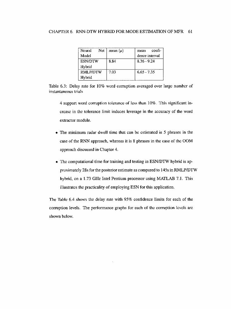
CHAPTER 6. RNN-DTW HYBRID FOR MODE ESTIMATION OF MFR 61
Neural Net mean (J.l) mean confi-Model dence interval
ESN/DTW 8.84 8.36-9.24 Hybrid
RMLP/DTW 7.03 6.65- 7.35 Hybrid
Table 6.3: Delay rate for 10% word corruption averaged over large number of instantaneous trials
4 support word corruption tolerance of less than 10%. This significant in
crease in the tolerance limit induces leverage in the accuracy of the word
extractor module.
• The minimum radar dwell time that can be estimated is 5 phrases in the
case of the RNN approach, whereas it is 8 phrases in the case of the OOM
approach discussed in Chapter 4.
• The computational time for training and testing in ESN/DTW hybrid is ap
proximately 28s for the posterior estimate as compared to 145s in RMLP/DTW
hybrid, on a 1.73 GHz Intel Pentium processor using MATLAB 7.1. This
illustrates the practicality of employing ESN for this application.
The Table 6.4 shows the delay rate with 95% confidence limits for each of the
corruption levels. The performance graphs for each of the corruption levels are
shown below.
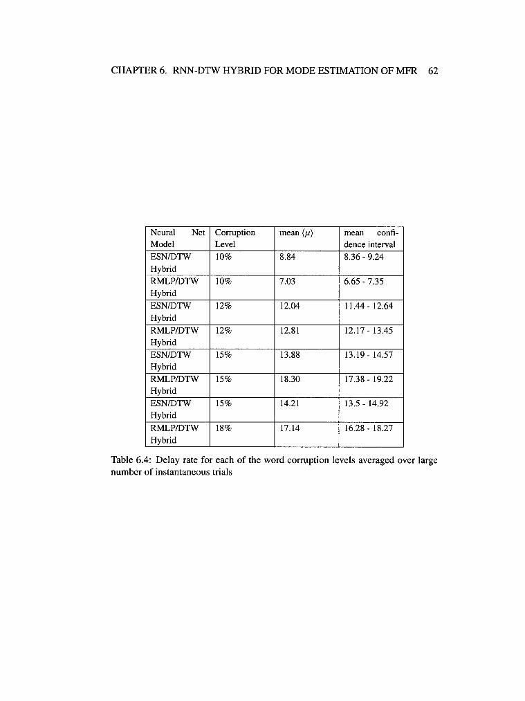
CHAPTER 6. RNN-DTW HYBRID FOR MODE ESTIMATION OF MFR 62
Neural Net Corruption mean (J.l) mean confi-Model Level dence interval
ESN/DTW 10% 8.84 8.36-9.24 Hybrid RMLP/DTW 10% 7.03 6.65- 7.35 Hybrid
ESN/DTW 12% 12.04 11.44- 12.64 Hybrid
RMLP/DTW 12% 12.81 12.17- 13.45 Hybrid
ESN/DTW 15% 13.88 13.19- 14.57 Hybrid
RMLP/DTW 15% 18.30 17.38- 19.22 Hybrid
ESN/DTW 15% 14.21 13.5- 14.92 Hybrid
RMLP/DTW 18% 17.14 16.28- 18.27 Hybrid
Table 6.4: Delay rate for each of the word corruption levels averaged over large number of instantaneous trials
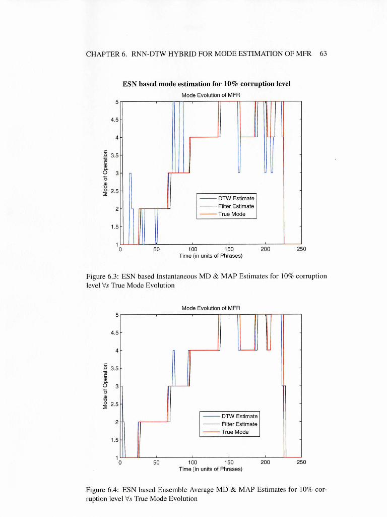
CHAPTER 6. RNN-DTW HYBRID FOR MODE ESTIMATION OF MFR 63
5
4.5
4
c 0 3.5 -~ <ll Q. 0 3 0 <ll "0 0 2.5 :2
2
1.5
1 0
ESN based mode estimation for 10% corruption level
Mode Evolution of MFR
I--
--DTW Estimate -- Filter Estimate --True Mode
50 100 150 200 Time (in units of Phrases)
250
Figure 6.3: ESN based Instantaneous MD & MAP Estimates for 10% corruption level Vs True Mode Evolution
Mode Evolution of MFR 5
4.5
4
c 0 3.5 ~ Qj Q. 0 3 0 <ll "0 0 2.5 :2
--DTW Estimate 2 -- Filter Estimate
-- True Mode
1.5
1 0 50 100 150 200 250
Time (in units of Phrases)
Figure 6.4: ESN based Ensemble Average MD & MAP Estimates for I 0% corruption level 'r:/s True Mode Evolution
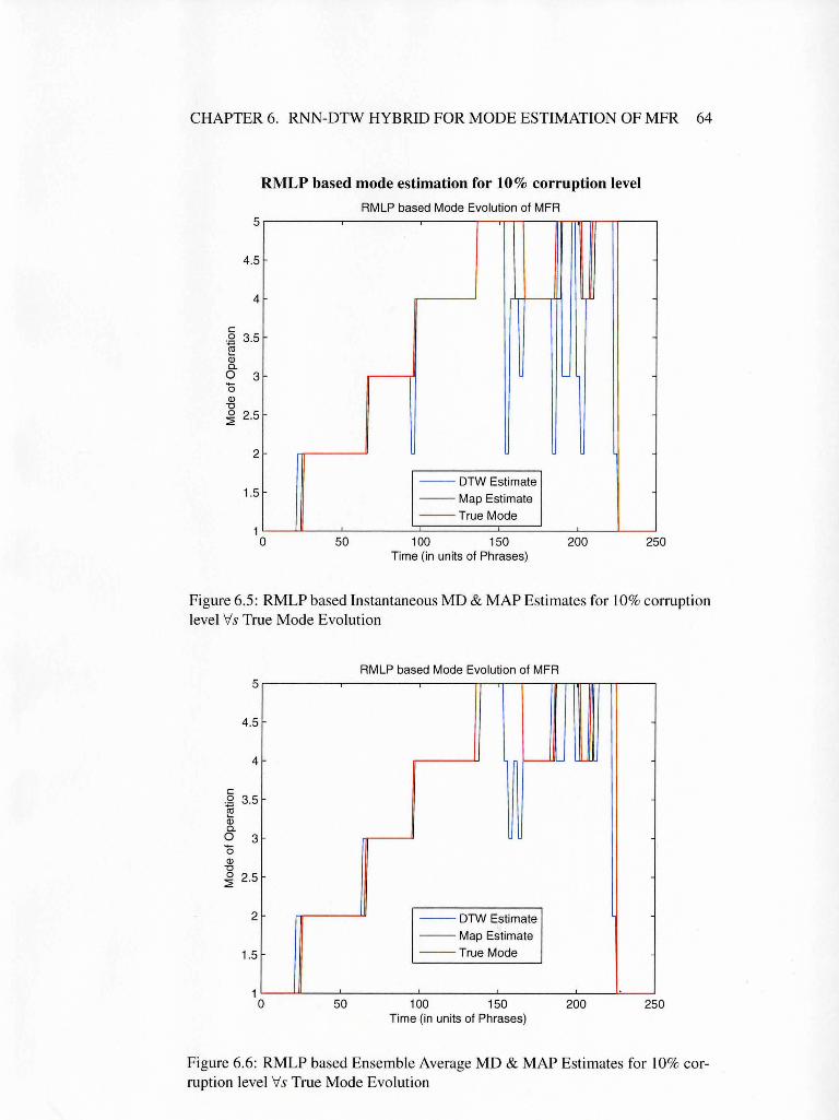
CHAPTER 6. RNN-DTW HYBRID FOR MODE ESTIMATION OF MFR 64
RMLP based mode estimation for 10% corruption level
AMLP based Mode Evolution of MFA 5.--------,---------.-----.--n-rr---n-mrm~.---,
4.5
4
c 0 3.5 ~ Q) a. 0 3 0 Q) -o ~ 2.5
2
1.5 --DTW Estimate --- Map Estimate --True Mode
1L__il __ ~------~======~==~--~--L__j 0 50 100 150 200 250
Time (in units of Phrases)
Figure 6.5: RMLP based Instantaneous MD & MAP Estimates for 10% corruption level Vs True Mode Evolution
AMLP based Mode Evolution of MFA 5
4.5
4 -
c 0 3.5 ~ Q; a. 0 3 0 Q) -o ~ 2.5
2 --DTW Estimate --Map Estimate
1.5 --True Mode
1 0 50 100 150 200 250
Time (in units of Phrases)
Figure 6.6: RMLP based Ensemble Average MD & MAP Estimates for LO% corruption level Vs True Mode Evolution
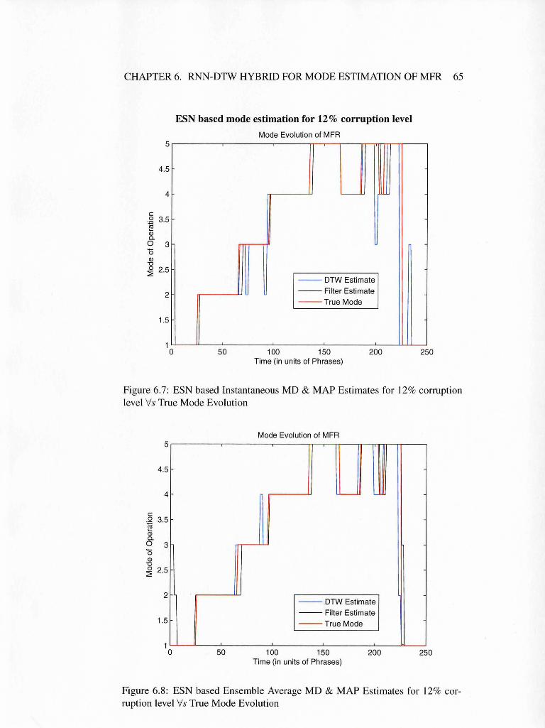
CHAPTER 6. RNN-DTW HYBRID FOR MODE ESTIMATION OF MFR 65
5
4.5
4
c 0 3.5 ~ Q) a. 0 3 0 Q) "0
~ 2.5
2
1.5
1 0
ESN based mode estimation for 12% corruption level
Mode Evolution of MFA
-- DTW Estimate
-- Filter Estimate --True Mode
50 100 150 200 Time (in units of Phrases)
250
Figure 6.7: ESN based Instantaneous MD & MAP Estimates for 12% corruption level Vs True Mode Evolution
Mode Evolution of MFA 5
4.5
4
c 0 3.5 ~ Q; a. 0 3 0 Q)
"0 0 2.5 ~
2 --DTW Estimate -- Filter Estimate
1.5 --True Mode
1 0 50 100 150 200 250
Time (in units of Phrases)
Figure 6.8: ESN based Ensemble Average MD & MAP Estimates for 12% corruption level Vs True Mode Evolution
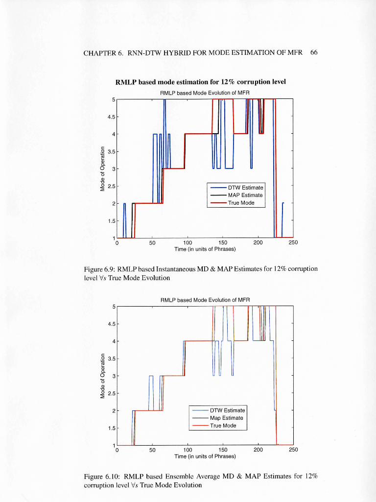
CHAPTER 6. RNN-DTW HYBRID FOR MODE ESTIMATION OF MFR 66
5
4.5
4
c 0 3.5 ~ Q) c. 0 3 0 Q)
"0 0 2.5 :2
2
1.5
1
RMLP based mode estimation for 12% corruption level
RMLP based Mode Evolution of MFR
-
--DTW Estimate --MAP Estimate --True Mode
0 50 100 150 200 Time (in units of Phrases)
250
Figure 6.9: RMLP based Instantaneous MD & MAP Estimates for 12% corruption level Vs True Mode Evolution
RMLP based Mode Evolution of MFR 5
4.5
4 I-- '----
c 0 3.5 -~ Q) c. 0 3 0 Q) "0 0 2.5 :2
2 --DTW Estimate --Map Estimate
1.5 --True Mode
1 0 50 100 150 200 250
Time (in units of Phrases)
Figure 6. 10: RMLP based Ensemble Average MD & MAP Estimates for 12% corruption level Vs True Mode Evolution
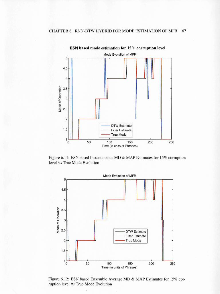
CHAPTER 6. RNN-DTW HYBRID FOR MODE ESTIMATION OF MFR 67
5
4.5
4
c 0 3.5 -~ Q) a. 0 3 0 Q)
"'0 0 2.5 :::2:
2
1.5
1 0
ESN based mode estimation for 15% corruption level
Mode Evolution of MFA
-- DTW Estimate -- Filter Estimate --True Mode
50 100 150 200 Time (in units of Phrases)
250
Figure 6.11 : ESN based Instantaneous MD & MAP Estimates for 15 % corruption level V s True Mode Evolution
Mode Evolution of MFA 5
4.5
4
c 0 3.5 -~
iii a. 0 3 0 Q)
"'0 0 2.5 :::2: --DTW Estimate
-- Filter Estimate 2 --True Mode
1.5
1 0 50 100 150 200 250
Time (in units of Phrases)
Figure 6.12: ESN based Ensemble Average MD & MAP Estimates for 15% corruption level Vs True Mode Evolution
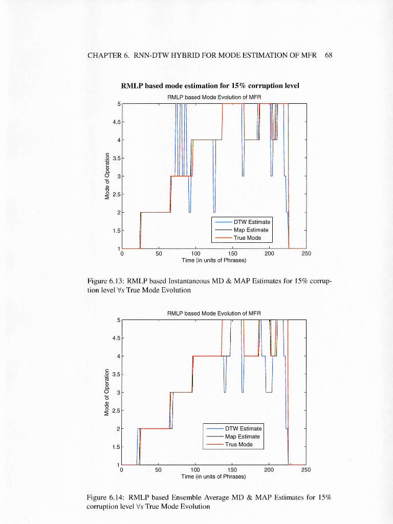
CHAPTER 6. RNN-DTW HYBRID FOR MODE ESTIMATION OF MFR 68
5
4.5
4
c 0 3.5 -~ Q) a. 0 3 0 Q) "0 0 2.5 ~
2
1.5
1
RMLP based mode estimation for 15% corruption level
AMLP based Mode Evolution of MFA
-- DTW Estimate -- Map Estimate --True Mode
0 50 100 150 200 Time (in units of Phrases)
250
Figure 6.13: RMLP based Instantaneous MD & MAP Estimates for 15% corruption level Vs True Mode Evolution
AMLP based Mode Evolution of MFA 5
4.5
4
c 0 3.5 ~ Qj a. 0 3 0 Q) "0 0 2.5 ~
2 --DTW Estimate --Map Estimate
1.5 --True Mode
1 0 50 100 150 200 250
Time (in units of Phrases)
Figure 6.14: RMLP based Ensemble Average MD & MAP Estimates for 15% corruption level Vs True Mode Evolution
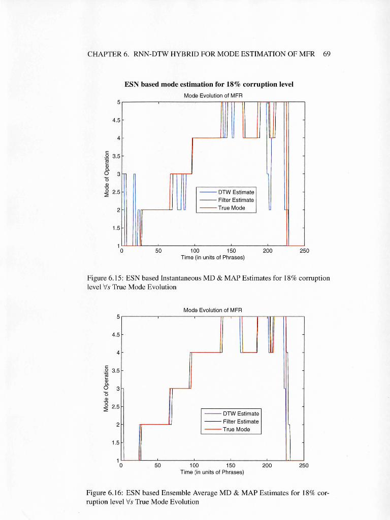
CHAPTER 6. RNN-DTW HYBRID FOR MODE ESTIMATION OF MFR 69
5
4.5
4
c 0 3.5 ~ QJ 0.. 0 3 0 QJ
"0
~ 2.5
2
1.5
1 0
ESN based mode estimation for 18% corruption level
Mode Evolution of MFA
--DTW Estimate -- Filter Estimate --True Mode
50 100 150 200 Time (in units of Phrases)
250
Figure 6.15: ESN based Instantaneous MD & MAP Estimates for 18% corruption level Vs True Mode Evolution
Mode Evolution of MFA 5
4.5
4
c 0 3.5
-~
Gi 0.. 0 3 0 QJ
"0 0 2.5 ~
--DTW Estimate
2 -- Filter Estimate --True Mode
1.5
1 0 50 100 150 200 250
Time (in units of Phrases)
Figure 6.16: ESN based Ensemble Average MD & MAP Estimates for 18% corruption level Vs True Mode Evolution
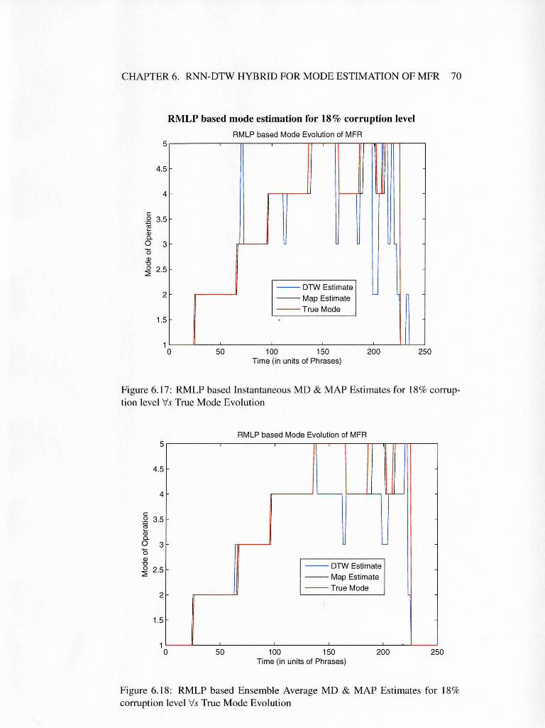
CHAPTER 6. RNN-DTW HYBRID FOR MODE ESTIMATION OF MFR 70
5
4.5
4
c 0 3.5
·~ (jj 0.. 0 3 0 Ql -o 0 2.5 ~
2
1.5
1
RMLP based mode estimation for 18% corruption level
RMLP based Mode Evolution of MFR
--DTW Estimate -- Map Estimate --True Mode
0 50 100 150 200 Time (in units of Phrases)
250
Figure 6.17: RMLP based Instantaneous MD & MAP Estimates for 18% corruption level Vs True Mode Evolution
RMLP based Mode Evolution of MFR 5
4.5
4 -
c 0 3.5
·~ (jj 0.. 0 3 0 Ql -o 0 2.5 ~
--DTW Estimate --Map Estimate -- True Mode
2
1.5
1 0 50 100 150 200 250
Time (in units of Phrases)
Figure 6. 18: RMLP based Ensemble Average MD & MAP Estimates for 18% corruption level Vs True Mode Evolution
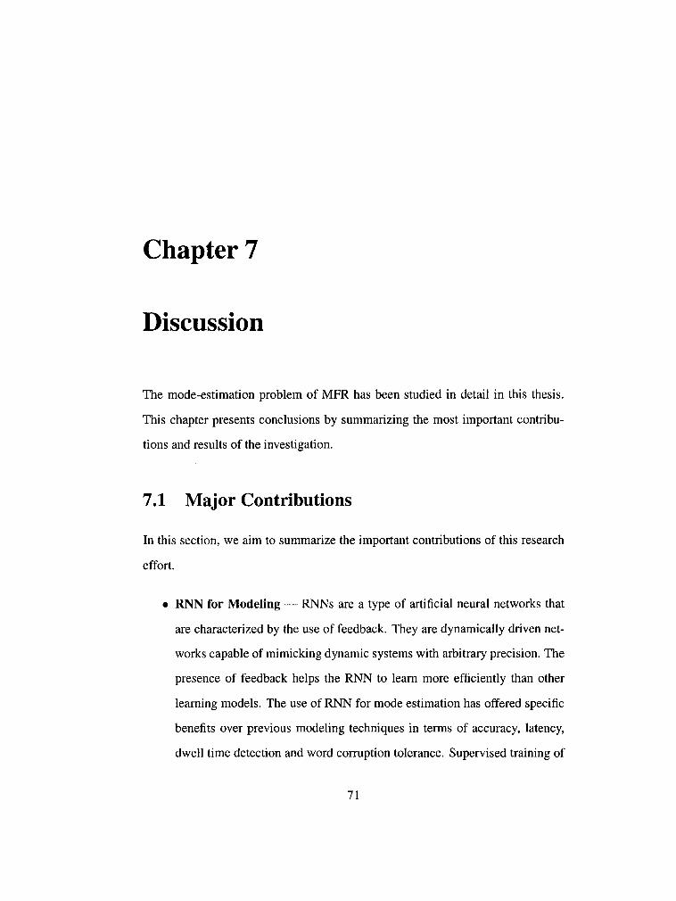
Chapter 7
Discussion
The mode-estimation problem of MFR has been studied in detail in this thesis.
This chapter presents conclusions by summarizing the most important contribu
tions and results of the investigation.
7.1 Major Contributions
In this section, we aim to summarize the important contributions of this research
effort.
• RNN for Modeling- RNNs are a type of artificial neural networks that
are characterized by the use of feedback. They are dynamically driven net
works capable of mimicking dynamic systems with arbitrary precision. The
presence of feedback helps the RNN to learn more efficiently than other
learning models. The use of RNN for mode estimation has offered specific
benefits over previous modeling techniques in terms of accuracy, latency,
dwell time detection and word corruption tolerance. Supervised training of
71
CHAPTER 7. DISCUSSION 72
the ESN and training of the RMLP by the EKF algorithm, which is also
supervised, are efficient in capturing the word generation mechanism of the
radar. This subsequently helps in estimating the operational mode of MFR
accurately.
• Single Model Approach - A single model approach is proposed to track
the operational mode of MFR. The mode estimation of MFR is achieved by
building a single RNN model to learn the underlying word generation mech
anism of the MFR through supervised training. A single model approach
overcomes the burden of building individual models for each operational
mode of MFR, which would prove to be a cumbersome task if the num
ber of operational modes is large. Thus a single model approach is more
practical to solve the MFR problem.
• Word Level Estimation - Since the MFR employs complex pulse struc
ture with the capability to perform multiple tasks, mode estimation becomes
very difficult at the pulse level. To overcome this difficulty and to keep the
signal processing complexity manageable, a hierarchial signal structure is
proposed, in which individual words extracted from the MFR pulses are
used for mode estimation. Mode estimation carried out in the word level,
which is subsequent to the pulse level, is less computationally intensive and
erroneous than pulse level processing.
• Improved Performance- The RNN-DTW hybrid presented in this inves
tigation has demonstrated improved performance over previous approaches
in the mode estimation of MFR. The significant performance improvements
include higher degree of reliability and accuracy, reduced latency rates,
CHAPTER 7. DISCUSSION 73
improved dwell time detection and most importantly higher word corrup
tion tolerance. The word corruption tolerance has been increased to 18%
in RNN-DTW hybrid from below 10% supported by previous techniques.
Computer simulations show that the RNN-DTW hybrid has not only over
come the limitations associated with the previous techniques, but has also
achieved it with comparable computational intensity.
7.2 Conclusion
This thesis presents a novel method, the RNN-DTW hybrid to estimate and track
the mode of operation of MFR accurately. Since the electromagnetic emissions
of the radar are very complex, a hierarchial signal architecture is proposed to
keep the signal processing complexity manageable. The mode estimation is then
performed at a higher level of the hierarchial signal architecture, known as the
word level.
The proposed methodology was tested for two RNNs, namely, the ESN and
RMLP. The RNNs are trained in a supervised manner to capture the underlying
word generation mechanism of the MFR. DTW is used as the post processor for
both RNN models. Minimum distance is the decision criterion used to estimate
the mode of operation. The phenomenon of occasional mode jumps of the min
imum distance estimate is mitigated by updating the probability of each opera
tional mode in a recursive fashion. This is achieved by using the knowledge of
the distance estimates and the prior mode transition probabilities in a grid filter
framework. Finally, the jump free estimate of the current operational mode is ob
tained in the MAP sense by maximizing the mode probability at that particular
CHAPTER 7. DISCUSSION 74
time instant.
Computer simulations conducted for both instantaneous and Monte Carlo tri
als show that the RNN approach performs better than the previous mode esti
mation techniques with increased corruption tolerance, reduced latency rates, im
proved dwell time detection and comparable run times. Among the two RNNs, the
results show that the performance of grid based ESN/DTW hybrid is much similar
to its RMLP counterpart in all the above mentioned performance criterion. How
ever, in terms of computation time the performance of the former is only about
one fifth of the latter. Since computation time may be an important parameter in
the threat analysis of MFR, it is considered to be the deciding factor between the
two RNN models. Therefore, we conclude that grid based ESN/DTW hybrid is a
suitable candidate for tracking the operational mode of the MFR, both in terms of
performance and computational complexity.
Bibliography
[1] C. Schleher, Introduction to Electronic Warfare, Artech House, UK,
1986.
[2] M. I. Skolnik, Introduction to Radar Systems, McGraw-Hill, NY, 2002.
[3] I. Arasaratham, "Tracking the Mode of Operation of Multi-Function
Radar," Master's Thesis, Dept. of Electrical and Computer Eng., Mc
Master University, Canada, 2006.
[4] R. G. Wiley, Electronic Intelligence: The Analysis of Radar Signals,
Artech House, UK, 1993.
[5] R. G. Wiley, Electronic Intelligence: Interception of Radar Signals,
Artech House, UK, 1985.
[6] N. Visnevski, "Syntactic Modeling of Multi Function Radar", PhD Dis
sertation, Dept. of Electrical and Computer Eng., McMaster University,
Canada, 2005.
[7] N. Visnevski, S. Haykin, V. Krishnamurthy, F. Dilkes, and P. Lavoie,
"Hidden Markov Model for Radar Pulse Train Analysis in Electronic
75
BIDLIOGRAPHY 76
Warfare", Proceedings of the IEEE Conference on Acoustics, Speech
and Signal Processing, Philadelphia, PA, Mar. 2005.
[8] S. Theodoridis and K. Koutroumbas, Pattern Recognition, Academic
Press, USA, 2003.
[9] S. Salvador and P. Chan, "Fast DTW: Towards Accurate Dynamic Time
Warping in Linear Time and Space", KDD Workshop on Mining Tempo
ral and Sequential Data, Dept. of Computer Sciences, Florida Institute
of Technology, FL, 2004.
[10] S. Haykin, Neural Networks: A Comprehensive Foundation, Prentice
Hall, NJ, 1999.
[11] H. Jaeger and H. Haas, "Harnessing Nonlinearity: Predicting Chaotic
Systems and Saving Energy in Wireless Communication", Science,
Apr. 2004, pp. 78-80.
[12] H. Jaeger,"A Tutorial on Training Recurrent Neural Networks, Cover
ing BPTT, RTRL, EKF and the Echo State Network Approach", ***,
2004.
[13] H. Jaeger,"Adaptive Nonlinear System Identification with Echo State
Networks" Advances in Neural Information Processing Systems 15, S.
Becker, S. Thrun, and K. Obermayer (Eds), MIT Press, Cambridge,
MA, 2003, pp. 593-600.
[14] H. Jaeger, "The Echo State Approach to Analysing and Training Re
current Neural Networks", GMD Report, German National Research
Center for Information Technology, 2001.
BIDLIOGRAPHY 77
[15] J. Matuszewski and L. Paradowski,"The Knowledge-Based Approach
for Emitter Identification", International Conference on Microwaves
and Radar, MIKON, 1998, pp. 810-814.
[ 16] P. J. Werbos, "Backpropagation Through Time: What it does and how to
do it", Proceedings of the IEEE, Vol. 78, Issue 10, Oct. 1990, pp. 1550-
1560.
[17] B. Ristic, S. Arulampalam, and N. Gordon, Beyond the Kalman Filter:
Particle Filters for Applications, Artech House, UK, 2004.
[18] G. V. Puskorius and L. A. Feldkamp, "Decoupled Extended Kalman
Filter Training of Feedforward Layered Network", International Joint
Conference on Neural Networks, Vol. 1, 1991, pp. 771-777.
[19] G. V. Puskorius and L.A. Feldkamp, "Neurocontrol of Nonlinear Dy
namical Systems with Kalman Filter Trained Recurrent Networks",
IEEE Transactions on Neural Networks, Vol. 5, 1994, pp. 279-297.
[20] R. J. Williams and J. Peng, "An Efficient Gradient Based Algorithm for
Online Training of Recurrent Network Trajectories", Neural Computa
tions, Vol. 2, 1990, pp. 490-501.
[21] S. Singhal and L. Wu, "Training Feed-Forward Networks with Ex
tended Kalman Filter", IEEE International Confrence for Acoustics,
Speech and Signal Processing, Glasgow, Scotland, 1989, pp. 1187-
1190.
BIBLIOGRAPHY 78
[22] R. E. Kalman, "A New Approach to Linear Filtering and Prediction
Problems", Transactions of ASME, Journal of Basic Engineering, Vol.
82, 1960, pp. 35-45.
[23] L. R. Rabiner, "A Tutorial on Hidden Markov Models and Selected Ap
plications in Speech Recognition", Proceedings of the IEEE, 77(2), Feb.
1989, pp. 257-286.
[24] J. E. Hopcroft, R. Motwani, and J.D. Ullman, Introduction to Automata
Theory, Languages and Computation, Addison-Wesley, MA, 2002.
[25] H. Jaeger, "Discrete-Time, Discrete-Valued Observable Operator Mod
els: A Tutorial", Tech. Report, GMD, Sankt Augustin, 1998.
[26] H. Jaeger, "Observable Operator Models for Discrete Stochastic Time
Series", Neural Computation, No.6, 2000, pp. 1371-1398.
[27] H. Jaeger, M. Zhao, K. Krettzhmar, T. Obesrtein, D. Popovinci, and
A. Kolling, "Learning Observable Operator Models via the ES Al
gorithm", New Directions in Statistical Signal Processing: from Sys
tems to Brains, (eds. S. Haykin, J. C. Principe, T. Sejnowski, and J.
McWhirter), MIT Press, Cambridge, MA, 2006.
[28] Y. Bengio, Neural Network for Speech and Sequence Recognition, In
ternational Thomson Publishing, 1995.
[29] Y. Xue, L. Yang, and S. Haykin, "Decoupled Echo State Network
with Lateral Inhibition", Elsevier Neural Networks, 20(3), Apr. 2007,
pp. 365-376.

BIBLIOGRAPHY 79
[30] N. Chomsky, "On Certain Properties of Grammars, Information and
Control", Vol. 2, Issue 2, Jun. 1959, pp. 137-167.