1

Tracking the Source of the Decline in GDP Volatility: An

Analysis of the Automobile Industry

by

Valerie A. RameyUniversity of California, San Diego and National Bureau of Economic Research

and

Daniel J. VineBoard of Governors of the Federal Reserve System

First Draft: December 2001This Draft: March 11, 2004

Abstract

Recent papers by Kim and Nelson (1999) and McConnell and Perez-Quiros (2000) uncover adramatic decline in the volatility of U.S. GDP growth beginning in 1984. Determining whetherthe source is good luck, good policy or better inventory management has since developed into anactive area of research. This paper seeks to shed light on the source of the decline in volatility bystudying the behavior of the U.S. automobile industry, where the changes in volatility havemirrored those of the aggregate data. We find that changes in the relative volatility of sales andoutput, which have been interpreted by some as evidence of improved inventory management,are in fact the result of changes in the process driving automobile sales. We first show that theautocorrelation of sales dropped during the 1980s, and that the behavior of interest rates may bethe force behind the change in sales persistence. A simulation of the assembly plants’ costfunction illustrates that the persistence of sales is a key determinant of output volatility. Acomparison of the ways in which assembly plants scheduled production in the 1990s relative tothe 1970s supports the intuition of the simulation._____________________

We are indebted to Edward Cho and Jillian Medeiros for outstanding research assistance and to George Hall for hisChrysler data. We have benefited from helpful comments from Garey Ramey, Mark Watson, Jeronimo Zettelmeyer,participants in the NBER Monetary Economics and Economic Fluctuations and Growth groups, the Hydra, GreeceWorkshop on Dynamic Macroeconomics, the UCSD Applied Lunch Group, John Haltiwanger and the participantsat the International Society for Inventory Research seminar in Atlanta, GA. Valerie Ramey gratefully acknowledgessupport from National Science Foundation Grant SBR-9617437 through the National Bureau of Economic Research,and National Science Foundation grant # 0213089. Opinions expressed here are those of the authors and not thoseof the Board of Governors of the Federal Reserve System.

2

I. Introduction

Recent papers by Kim and Nelson (1999) and McConnell and Perez-Quiros (2000)

uncover a dramatic decline in the volatility of the U.S. economy beginning in 1984. The

volatility of GDP growth since 1984 has been 50 percent lower than it was in the post-war period

before 1984. Interestingly, statistical tests point to a structural break in the first quarter of 1984

rather than to a gradual decline. The phenomenon also appears to extend beyond U.S. borders.

Blanchard and Simon (2001) and Stock and Watson (2003a) show that all G-7 countries save

Japan have experienced a decline in volatility in recent periods, though the timing and nature of

the declines vary by country.

This discovery raises an important question: Has output volatility declined in a

meaningful and permanent way, or have we simply enjoyed a reprieve from the turbulence of the

1970s and early 1980s? Possible answers to this question depend on which of the three leading

explanations for the decline in volatility is most accurate: (1) Good Luck, (2) Good Policy, or

(3) Structural Change. The "Good Luck” hypothesis argues that the decline in volatility is a

result of a fortuitous decline in the volatility of shocks hitting the economy (e.g. Ahmed, Levin,

and Wilson (2000), Stock and Watson (2002)). Advocates of the “Good Policy” hypothesis

argue that a systematically more decisive and more transparent monetary policy has been the key

source of the decline in volatility of the U.S. economy (e.g. Clarida, Galí, and Gertler (2000),

Boivin and Giannoni (2002) and McCarthy and Zakrajšek (2003)). Finally, the “Structural

Change” hypothesis refers to the innovations in manufacturing technology and inventory

management that allow smooth production along the supply chain (e.g. Kahn, McConnell and

Perez-Quiros (2002) and Irvine and Schuh (2002)). This potential source has recently received a

lot of attention, as the decline in the volatility of aggregate output exceeds that of final sales.

Despite a rapidly developing literature in this area, answering this question in a definitive

way has proven to be difficult. First, a significant reduction in volatility has been discovered

almost universally across the U.S. economy. Aggregate volatility patterns thus provide little help

in narrowing the focus to a particular change in the economic environment or to the contribution

3

of a particular input.1 Second, the conclusions reached from time-series analysis on aggregate

data have been difficult to interpret. The reduction in GDP volatility seems to stem from a

decline in the volatility of shocks, which are typically the forecast errors that result from a vector

autoregression model of the U.S. economy. To further associate these forecast errors with

measurable shocks, such as monetary and fiscal shocks, productivity shocks, supply shocks, etc.,

however, has not met with success.2

This study addresses the decline in U.S. GDP volatility in the context of decisions made

at the plant level in an industry at the forefront of this change – the U.S. automobile industry.

Not only has the automobile industry experienced a sharp decline in its volatility during the

1980s, but it is also an industry often examined by economists such as Blanchard (1983) to

understand the interaction between inventories and the volatility of output. Using aggregate

automobile industry data as well as a new disaggregated dataset that tracks weekly production

scheduling at automobile assembly plants between 1972 and 2001, we investigate the extent to

which the decline in volatility stems from structural changes in the process governing sales

versus structural changes in the process governing production. We conclude that the decline in

output volatility is linked to (1) a decline in the measured persistence of sales shocks and (2)

plant-level non-convexities in production scheduling. In particular, sales are far less serially

correlated after 1984 than they were during the 1970s and early 1980s, and interest rates appear

to be a source of the change. We demonstrate that an inventory model involving non-convex

costs predicts that a decline in the persistence of sales shocks leads to a decline in the variance of

production relative to the variance of sales and to a decline in the covariance of inventory

investment and sales. Finally, we show that the type of data used by other researchers may hide

a change in persistence in other parts of the economy. Thus, recent evidence suggesting no

change in the persistence of final sales overall may be an artifact of the data.

The organization of this paper is as follows: Section II explains the connection between

output volatility, inventory investment and improvements in information and production

1 Stock and Watson (2002) test 168 U.S. macroeconomic time-series and discover the pervasiveness of this volatilitydecline in measures of output, employment, investment and inflation. Manufacturing has been more impacted thatservices, however, and durable goods output volatility has experienced a particularly steep reduction.

2 Stock and Watson (2002) search over several identifiable shocks in the U.S., and Stock and Watson (2003a) do soagain for all G7 countries. In both cases, the behavior of observable shocks is quite different from that of theforecast errors of GDP growth.

4

technologies. Section III demonstrates that the automobile industry is suitable for this case study

and presents evidence that the process governing automobile sales has changed noticeably in the

post-1984 period. Section IV addresses how a change in sales persistence interacts with

production decisions in a simulation featuring the non-convex production costs typical in this

industry. Section V confronts our theory with a panel of production scheduling variables across

U.S. assembly plants. Section VI discusses whether the automobile industry results may be

extended to the rest of the economy, and Section VII concludes.

II. The Information Technology Explanation

Innovations in information and production technology have transformed U.S.

manufacturing in many important ways in recent decades. The current question is whether

technological change also underlies the moderation in GDP volatility. Kahn, McConnell and

Perez-Quiros (2002), hereafter KMPQ, give perhaps the most compelling evidence that it has.

They argue that the decline in GDP volatility is most closely matched in magnitude and in timing

by a similar reduction within the durable goods sector.3 KMPQ further argue that the adoption

of new machine tool technologies and inventory control systems occurred most rapidly during

the 1980s within the durable goods sector. Thus, the “Information Technology Hypothesis”

posits that production lines and inventory distribution systems now respond more rapidly to sales

conditions than they used to, and this improvement has moderated the response of production to

sales shocks.

Two of the most striking pieces of statistical evidence presented by KMPQ in favor of

this hypothesis are the differential declines in final sales versus production volatility and the

changing covariance of inventory investment with final sales. To see how this evidence relates

to inventory management, consider the standard inventory identity t t tY S I= + ∆ , where Y is

production, S is sales, and ∆ I is the change in inventories. For stationary variables, we have the

following relationship between the variance of production and the variance of sales:

3 Kim, Nelson, and Piger (2001) present evidence of structural breaks across broad sectors. McConnell and Perez-Quiros (2000), Warnock and Warnock (2000), and Kahn, McConnell, and Perez-Quiros (2002) offer evidence thatthe durable goods sector plays the most important role. Stock and Watson (2002) claim residential fixed investmentplayed an equally large role as durable goods production.

5

(1) ( ) ( ) ( ) 2 ( , )t t t t tVar Y Var S Var I Cov S I= + ∆ + ∆ .

The standard version of the production-smoothing model of inventories predicts that the variance

of production should be less than the variance of sales. Thus, the covariance of inventory

investment and sales should be negative. Historically, the opposite has been true.

KMPQ apply a version of this formula to growth rates of chain-weighted production,

sales, and inventory investment in the durable goods industry and find that the variance of

production fell by a much larger share from the pre-1984 period to the post-1984 period than did

the variance of final sales. Moreover, the covariance of inventory investment and sales in

durable goods turned from being positive in the early period to negative in the post-1984 period.4

Instead of contributing to the volatility of the economy as they once did, inventories now appear

to stabilize production.

The connection between the “Information Technology (IT)” hypothesis and the

covariance of inventories with sales is as follows: Information technology innovations, such as

electronic scanning of bar codes, allow for automatic restocking based on real-time sales

information and facilitate higher efficiency along the entire supply line. Elements of flexible

manufacturing, such as computer numerically controlled machine tools, have additionally led to

a reduction in set-up times required to produce different specifications of goods. This change in

set-up costs lowers optimal batch size, which varies inversely with inventory levels. Both of

these innovations would be expected to reduce desired inventory-sales ratios. A reduction in the

desired inventory-sales ratio should weaken or eliminate the tendency for inventories to be so

pro-cyclical, and hence so destabilizing.

The volatility and covariance measurements suggest that an explanation of the decline in

aggregate output volatility must be consistent with the following observations: (1) The source

must have particularly strong effects on the durable goods sector as opposed to nondurables and

services; and (2) the effect on production should be more pronounced that the effect on final

sales. KMPQ argue that these observations cast doubt on the “better monetary policy”

explanation since one should expect it to work mostly through sales.

4 Golob (2000) first discovered this switch in the sign of the covariance term.

6

While the changes observed in variance and covariance are consistent with the hypothesis

that information technology and inventory management are the source of the decline in volatility,

this conclusion is not supported by specific studies of inventory control methods and their effects

on output volatility. McCarthy and Zakrajšek (2003) cite numerous articles from the operations

research literature that do draw a connection between improved inventory control methods and a

lower inventory-to-sales ratio at various stages of processing, but fail to find significant effects

on output volatility. Similarly, Feroli (2002) models the optimal inventory-to-sales ratio as a

function of input prices, where inventories serve as an input to production that is substitutable

with equipment and software. While declines in the relative user cost of information technology

can explain a declining inventory-to-sales ratio quite well, the impact on output volatility is

minute.

Patterns in U.S. inventory data also pose two puzzles for the IT hypothesis. The first is

why technology adoption, which usually follows an S-curve, should show up as a one-time

structural break in volatility. The second concerns the inventory-sales ratio. As discussed above,

we would expect information technology innovations to reduce both the inventory-sales ratio and

the volatility of output in a similar way if they were the source of these changes. The data do not

give such a clear picture.

Figure 1 shows the ratio of nonfarm inventories to final sales since 1947. The data are in

chained dollars, which best measure the real trend since the current-dollar ratio’s trend is driven

by relative price changes (see Ramey and Vine (forthcoming)). Two distinct features in the

graph are important. First, there is a large run-up in the inventory-sales ratio that begins in the

late 1960s and lasts through the early 1980s. Second, there is an overall decline in the inventory-

sales ratio in the early 1980s through the present. While some industries may currently hold

historically low levels of inventory relative to sales, the aggregate inventory-sales ratio since the

early 1980s is still higher than it was during the 1950s and 1960s. KMPQ demonstrate that the

volatility of GDP and durable goods was approximately equal across the periods 1953–1968 and

1969–1983, before falling in 1984. Thus, the behavior of the inventory-sales ratio does not line

up very closely with the changes in volatility over time.

In sum, while the changes in relative variances and covariances are consistent with a

change in production management, other parts of the story are not necessarily consistent with the

7

data. As we show below, even the observed changes in relative variances and covariances are

not necessarily indicative of changes in production management.

III. Structural Change in the U.S. Automobile Industry

As noted by KMPQ, the way in which output volatility declined says a great deal about

what may have lead to this change. Before we discuss the ways in which sales volatility impacts

production volatility as agents minimize an inter-temporal cost function, this section studies

historical patterns in the volatility of production, sales, and inventories in the automobile

industry. We first show that the automobile industry exhibits volatility changes that are even

more dramatic than the aggregate, but qualitatively similar. We then show that other features of

aggregate inventory and production behavior are also present in the automobile industry.

Finally, we uncover a structural change in the process governing sales.

III.A Variances and Covariances of Production, Sales and Inventories

Table 1 shows the volatility of output growth in the aggregate economy as well as in the

key sectors of durable goods and motor vehicles. Following the strategy of McConnell and

Perez-Quiros (2000), we first test the variance of quarterly real (chain-weighted) motor vehicle

output growth for a structural break. The estimated break date occurs in the first quarter of 1984,

which corresponds to the break-date discovered by McConnell and Perez-Quiros (2000) for the

volatility of aggregate GDP. All variables are 1996 chain-weighted data from the NIPA

accounts of the BEA, and volatility is measured as the standard deviation of annualized growth

rates. The analysis begins in 1967 because of constraints on the availability of data for the motor

vehicle sector. As the first row of the table shows, the volatility of aggregate GDP growth has

declined by 53 percent from the pre-1984 period to the post-1984 period. 5 The decline for

durable goods is just under 50 percent while the decline for motor vehicles is 60 percent. The

last row shows that the decline in GDP volatility is slightly muted when motor vehicles are

excluded.

5 The volatility of aggregate GDP growth in the truncated early period is similar to the volatility of the extendedperiod from 1953 – 1983 as shown in Kahn, McConnell and Perez-Quiros (2002).

8

The results of this variance comparison suggest that the motor vehicle industry represents

an ideal case study of the decline in volatility. Its volatility behavior is similar to, but more

dramatic than, the behavior of GDP and durable goods overall. Thus, understanding the decline

in volatility in the automobile industry is likely to shed light on the decline in aggregate

volatility.

Another reason to study the automobile industry is the high quality of its data. While

Table 1 uses quarterly chain-weighted data for comparison purposes with aggregate GDP, data

for the motor vehicle sector are available in physical units and at higher frequencies. Not only

do physical unit data have the advantage that they do not suffer from index number problems as

one compares inventories, production and sales numbers over a long period of time, but, as we

demonstrate later in the paper, physical unit data can reveal time series properties that are hidden

by chain-weighted data. Thus, we use physical unit data for the remainder of the analysis.

Figure 2 depicts monthly sales and production of domestic passenger cars and light trucks

in the U.S. from 1967:01 through 2003:12, using physical unit data.6 Several features in these

plots are noteworthy. First, car production is less volatile in the late portion of the sample than in

the early portion. A second feature visible in Figure 2 is the difference between the secular

trends for passenger car sales, which have no trend, and light truck sales, which have grown

steadily since 1980. Since there are obvious differences in the conditional means of these market

segments, we treat them separately in most of the analysis.

In order to investigate whether the automobile industry displays changes in inventory,

production and sales behavior similar to the changes in durable goods discovered by KPMQ,

Table 2 reports the variance decomposition for physical unit data on cars and trucks in the U.S.

from 1967:01 through 2003:12.7 One important difference between the time-series properties of

physical unit data and NIPA data used in other studies is that stationarity tests on the logarithm

of physical unit variables reject a unit root in favor of a deterministic trend, with perhaps a break

in trend around 1984 for trucks. Thus, variance here is based on deterministically detrended 6 Data for light truck production is not available before 1977. The data appendix describes the data sources for all ofthe data used.

7 The variances and covariances do not add up because we have excluded imports and exports to and from Canadaand Mexico. When these elements are included in the analysis, production volatility drops even further as the newBig Three plants in Mexico produce in a fashion that is negatively correlated with U.S. production. U.S. Exports toCanada and Mexico have little impact on the variance of sales. While import/export activity within North Americaraises additional interesting questions, it further augments the results obtained here and does not cause them.

9

data.8 Within the class of trucks, we would also prefer to focus solely on light trucks, since they

are mostly a consumer product like cars. Unfortunately, complete data on production and

inventories back to 1967 are only available for all trucks. Heavy trucks represented 22 percent

of truck production in 1967 but only 7 percent in 2000 as light truck production grew.

Consider first the case of cars, shown in the top panel of Table 2. Both seasonally

adjusted and unadjusted data show that the variance of production and the variance of sales fall

after 1984. Moreover, the variance of production falls by a larger percentage than sales, and the

covariance of inventory investment with final sales become more negative after 1984.

The results for trucks, shown in the bottom panel of Table 2, are similar in the seasonally

adjusted data, but not in the unadjusted data. In the unadjusted data, the variances of both

production and sales falls in the second period, but the variance of production falls by

proportionally less than the variance of sales so that the variance of production relative to sales is

higher in the second period. As is evident in Figure 2, the seasonality of light truck production is

much greater in the second period. As trucks were increasingly marketed as passenger vehicles,

production fluctuations due to model year changeovers became more pronounced. In both

adjusted and unadjusted data, however, the covariance of inventory investment with final sales

does become more negative after 1984, just as in the case of cars.

Thus, physical unit data in the automobile industry exhibit the same changes in the

relative variances and covariances highlighted by KPMQ in the chain-weighted durable goods

data. The automobile industry has also implemented many of the technological changes

showcased by KMPQ in their advocacy of the “Information Technology Hypothesis.” It

developed many of the advances in assembly line technology and was one of the first industries

to adopt just-in-time inventory management in the 1980s. Therefore, if advances in information

technology have revolutionized the fundamentals of U.S. manufacturing and distribution, and

have delivered unprecedented economic stability as a consequence, a natural place to look for

plant-level evidence is within the automobile industry.

Yet, the lack of a trend in the inventory-to-sales ratio is even more apparent within the

automobile industry than within the entire nonfarm sector. Figure 3 depicts this ratio in terms of

8 To be specific, we calculate the variances and covariances of the terms in Tt

tTt

tTt

t

YI

YS

YY

ˆˆˆ∆

+= , where

( )tY Tt ⋅+= 10

ˆˆexpˆ ββ and the β’s are the estimated parameters of a regression of log(Yt) on t.

10

the number of month’s worth of sales (in physical units) in the domestic inventory stock of cars

and light trucks.9 While this ratio shows a great deal of seasonal and business cycle variation,

the average has been remarkably stable. Thus, the behavior of inventory-sales ratios does not

support this version of the information technology story.

It is therefore interesting to explore an alternative explanation for the changes in

production and sales volatility. In particular, is it possible that the decline in production

volatility relative to sales stems from changes in the nature of the sales process rather than from

changes in the structure of production and inventories? We investigate this possibility in several

steps. The next subsection first uncovers changes in the sales process. The remainder of the

paper then demonstrates how changes in the sales process can explain the observed patterns

without recourse to structural change in the way firms manage production.

III.B Persistence of Aggregate Motor Vehicle Sales

The decrease in the volatility of both U.S. motor vehicle production and sales depicted in

the tables above arises from two potential sources: (1) a reduction in the magnitude of shocks to

these series, and (2) a change in the dynamic processes that propagate these shocks. Since

production decisions are made in accordance with forecasts of future sales, the volatility of

production depends not only on the variance of the shocks to the sales process, but also on the

persistence of these shocks (see Blanchard (1983)). Additional insight is therefore found by

comparing the persistence and volatility of sales shocks between the two periods. Within the

automobile industry, such an exercise reveals that the sales shocks since 1984 have been less

persistent than those prior to 1984.

Consider the following univariate model of the process for monthly domestic sales data

from 1967:1 through 2003:12:

(2) log( ) log( ) log( )1 1 2 0 1 1 2Sales Sales trend D D Sales D trendt o t t t t t tt tα α α β β β ε= + ⋅ + ⋅ + ⋅ + ⋅ ⋅ + ⋅ ⋅ +− −

where ( )tDNt ⋅+ 32,0~ βσε

9 Because data for inventories of light trucks are not available before 1972, the pre-1972 numbers are for cars only.Inventory-sales ratios of cars and light trucks are very similar.

11

and 1:1984for 11:1984for 0

≥=<=

tDtD

t

t .

This model allows a change in 1984:1 for all parameters, which include the coefficient on

lagged sales, the constant, the slope of the trend, and the variance of the residual. We estimate

this model via maximum likelihood for cars alone, light trucks alone, and for the combination of

cars and light trucks, which we call “motor vehicles.” In all cases the regression is estimated

with the logarithm of seasonally adjusted unit sales from the BEA.

Table 3 shows the results of this exercise, and the coefficient estimates indicate

significant changes have occurred in the process governing sales. The constant term and the

lagged sales coefficient are different across the two periods for all three aggregates. The trend

(which is not significant for the entire period) changes in the cases of light trucks and motor

vehicles. As for the variance of the shocks, there is a significant decline for light trucks, but not

for cars or the motor vehicle aggregate.

Of particular interest to our analysis is the change in the coefficient on lagged sales,

which measures the persistence of shocks to monthly sales. For all three vehicle categories the

first-order autocorrelation of sales falls between the early and the late periods. For passenger

cars this parameter falls from 0.85 to 0.55, and for trucks it falls from 0.9 to 0.7. When all motor

vehicles are grouped together, this estimate declines from almost 0.9 to 0.6.

This reduction in the serial correlation of car and light truck sales in the time domain is

also visible in the frequency domain, where the spectral density portions out total variance

among cycles of various frequencies. Figure 4 plots the spectral densities for U.S. monthly sales

of domestic cars (left side) and light trucks (right side) in physical units for the pre- and post-

1984 periods in the upper set of graphs.10 In the lower graphs, the solid line is the log ratio of the

two densities (early-to-late) at each frequency, and the dashed line is the log ratio of the total

variance in the two periods, which represents the change in the average height of the spectra.

Thus, frequencies for which the spectral ratio is greater than the variance ratio contribute more

than proportionately to the reduction in total variance. Frequencies for which the spectral ratio

lies below the variance ratio represent cycles that contribute less than proportionately to the

10 Spectral densities are constructed for sales as the deviation from trend of the logarithm of physical units. Thedensities are smoothed with the Bartlett kernel with window length equal to the square root of the sample size.

12

decline in total variance. When the spectral ratio lies below zero, cycles in this range of

frequencies actually cause more variance in the late period than in the early period.

In the case of cars, the total sales variance attributable to cycles with frequencies below

0.4×π are markedly lower in the post-1984 period than in the pre-1984 period, while cycles with

higher frequencies appear to have increased in variance. A frequency of 0.4×π in monthly data

corresponds to a period of five months. In the case of light trucks, the log ratio of early-to-late

spectra lies above zero at all frequencies, but the variance decline again is particularly stark at

lower frequencies. These observations in the frequency domain are equivalent to the reduction

in serial correlation measured in the time domain above for car and light truck sales, and to the

reduction in innovation variance measured for light truck sales.

To determine whether more disaggregated sales data also show a change in persistence,

the AR(1) model is estimated on unit sales at the company and division levels. Ideally, one

would like to examine sales at the assembly-plant level, since this is most important for

production scheduling. The distribution of models across plants, however, makes it difficult to

calculate plant-level sales. Not only does each assembly plant source multiple vehicle models,

but most models are produced by several plants as well, and companies frequently shift models

across plants. While monthly sales are available at the model level, these are often not suitable

for analysis because many have short life cycles, and these life-cycle patterns affect the estimates

of persistence.

Thus, Equation 2 is estimated with sales for the companies and divisions that exist in both

periods. Because disaggregated sales data are available only for cars in the earlier period, we

estimate the equation only for cars and not light trucks. Table 4 displays the results of this

disaggregated exercise.11 The decline in the persistence of sales shocks is similar for the

division-level data for General Motors and Ford. Every division shows a decline in persistence,

with magnitudes similar to those found for the aggregate for cars. Only a few cases show any

11 Because strikes have large effects on particular companies, we include a dummy variable for each month affectedby the strike plus the month afterward. (See the data appendix for details on strike dates.) The econometric modelis otherwise the same as the one used for the aggregate industry data. Monthly sales are seasonally adjusted with theBEA’s seasonal adjustment factor for cars.

13

significant change in the variance of the innovations.12 Chrysler Corporation, however, is an

exception. Only one of its divisions shows a marginally significant change in persistence.

In summary, for aggregate motor vehicle sales as well as for most company divisions, the

sales process in the post-1984 period returns to its mean much more quickly following a surprise

than was previously the case in earlier decades. It is also clear that most of the change in the

unconditional variance of sales described in the tables above comes from a change in the

propagation mechanism for sales rather than in the variance of sales shocks.

These results beg the question: why did the persistence of automobile sales decline? One

might suspect that the change in the sales process owes to changes in foreign trade. For

example, domestic sales of domestically produced vehicles include not only the sales of Big

Three vehicles, but also foreign nameplates that are produced domestically. Since the number of

the vehicles in this category has grown steadily during the 1990s, one might suspect that changes

in the definition of “domestic sales” are responsible for the change in their persistence. When

estimating the sales process of Big Three-only vehicles, however, the first-order autocorrelation

declines by 0.33, an almost identical amount to the estimates for all domestic sales. The same is

true when the definition of sales is expanded to domestic sales of all autos (including imports),

and when exports are included in total sales of domestic manufacturers. Thus, including or

excluding imports, exports and transplants does not change the basic results.

Ideally, one would do a structural analysis of a dynamic stochastic equilibrium model of

this durable goods oligolopoly to determine the source of the change. Data and space limitations

prevent us from doing a full structural analysis here. Instead, we offer some reduced form

evidence that may be suggestive of the source of the decline.

Likely candidates for the change in sales persistence are changes in the variables that

affect automobile demand, such as: (1) firms’ pricing behavior; (2) interest rates, perhaps due to

changes in the conduct of monetary policy; and (3) aggregate income. Suppose that automobile

sales depend on prices, aggregate income, interest rates, and an unobservable shock. When we

estimate a univariate AR process on auto sales alone, the estimated autocorrelation depends on

the data generating processes of these other variables as well as shocks to demand. Suppose that

automobile companies began to aggressively offer incentives and price discounts in the 1980s on

12 We do not put as much weight on the change in variance estimates because of the inclusion of the strike dummyvariables. All of the major strikes occurred in the early period, and we used 13 dummy variables to eliminate theireffects. The dummy variables serve to decrease the estimated variance of the innovation.

14

certain vehicles to rekindle sagging demand. If these price incentives represent a significant

change of practice, are used only at key points in time and have been successful in their aim, then

sales shocks in the univariate model would appear less persistent. Alternatively, if the monetary

authority has become more aggressive in using interest rates to respond to underlying shifts in

the economy that also affect automobile sales, then the measure of sales persistence in the

univariate model would again appear to have declined.

To determine whether any of these variables can account for the reduction in the

autocorrelation of sales observed above, we augment Equation 2 (using aggregate automobile

sales) with the current value and four lags of real automobile prices, real income, and nominal

interest rates.13 Assuming that automobile firms do not adjust their prices to the current month’s

sales shock, this equation can roughly be viewed as a demand equation. The aim of this exercise

is to test whether including any of these other variables makes the estimated persistence

parameter constant across the periods, thus indicating that the behavior of the extra variable was

the source of the difference.

Table 5 displays the results. The first row shows the estimated change in persistence for

the baseline with no other variables. For all classes of vehicles, the change in the persistence

across periods is significantly negative. The second row adds real motor vehicle prices. For

every class, the estimates are similar to the baseline and remain negative and significant. The

third row adds real income instead, which does reduce the magnitude of the change after 1984,

but the estimated change is still statistically significant. The results in the fourth row indicate

that the interest rate has the largest impact on the change in the AR(1) estimate. The magnitude

of the change falls noticeably relative to the baseline, and 1984 no longer represents a

statistically significant break date for cars or for all motor vehicles. These changes become even

smaller when all three variables are included. For cars and motor vehicles, the estimates are less

than half what they were in the baseline case and are not significant. In the case of light trucks,

the estimates are less than in the baseline case, but are still significant.

In summary, it appears that the change in persistence in sales owes in part to the behavior

of interest rates and perhaps income over the two periods. Surprisingly, including prices does

not have any explanatory power.

13 The demand for automobiles should depend on the rental cost in theory. Rental cost variables have lessexplanatory power than the components (interest rates and prices) entered separately.

15

IV. The Effect of Sales Persistence on Production Decisions

The crux of the IT hypothesis proposed by KMPQ rests on technological innovations in

the production process that change the way production is scheduled and inventories are managed,

given a fixed sales process. Their presentation of evidence implicitly assumes there is a fixed

relationship between the variance of production and the variance of sales in the absence of

structural change. In this section, we show how a change in the sales process alone modifies the

relationship between production, inventories and sales. This is true in the standard production

smoothing model when cost functions are convex (see Blanchard (1983), Ramey and Vine

(2003b)), but is more likely when cost functions are non-convex. Here we examine the more

realistic plant-level model with non-convex costs and lumpy production margins. Specifically,

we show that a decline in the persistence of sales shocks decreases the relative variance of

production over sales even without IT effects on production scheduling. Using a model

calibrated to the cost parameters of the U.S. automobiles industry, we show that the sales

persistence changes found in the data are sufficient to explain the changing relative volatilities of

production and sales.

IV.A Production Margins in Automobile Assembly Plants

In order to understand the sources of output volatility and the inventory management

techniques in the automobile industry, it is critical to first understand the institutional structure of

the automobile industry, its labor union, and the mechanical processes involved on the assembly

line. Managers of auto assembly plants have several margins at their disposal to meet production

quotas, many of which involve altering the period of production as opposed to the rate of

production.

Let Qit represent the monthly output volume for plant i. Qit is then a product of the

following margins: (1) the number of weeks in month t the plant is open; (2) the days per week

the plant operates; (3) the number of shifts working each day; (4) the length of each shift; and (5)

the line speed in terms of jobs per hour. This is shown in Equation 3.

(3)hourjobs

shifthours

dayshifts

weekopen days

monthopen weeks ××××=itQ

16

The institutional structures in automobile manufacturing have various implications for the

marginal costs of using and for the fixed costs of changing these margins. Aizcorbe (1990,

1992), for example, documents the implications for marginal cost found in the labor contract

between automobile manufacturers and the United Auto Workers. Bresnahan and Ramey (1994)

and Hall (2000) both study the ways in which production margin changes impact the volatility of

plant output. A conclusion that is common to these as well as other automobile industry studies

is that the constraints placed on production scheduling by union rules and the high cost of

retooling an assembly line make the plant’s cost function non-convex over many ranges of

output.

Consider first the number of hours an assembly plant works each week. Changes in

regular (non-overtime) hours most often take the form of closing the plant for an entire week.

This is called intermittent production, which is often preferable to operating a curtailed schedule,

called a short week, because plants are required by union contract to pay short-week

compensation to workers with at least one year of service. This is 85 % of a workers' regular pay

for each hour less than 40 they did not work. Closing the plant for the entire week, on the other

hand, entails laying workers off, in which case they receive 95% of their straight week pay

through a combination of state Unemployment Insurance (UI) and Supplemental Unemployment

Benefits (SUB).14

The length of a workweek may be extended temporarily with overtime hours. Overtime

hours take the form of one or two extra hours at the end of a regular eight-hour shift or as a Sat-

urday shift. Employees who work more than eight hours per day or more than forty hours per

week receive a 50% wage premium for the extra hours. Overtime hours are intended to be

temporary and assembly plants are prevented from using overtime permanently in lieu of hiring

additional workers. Frequent discontinuous spells of overtime, however, are not uncommon.

Long-term adjustments to production may involve adding or dropping the night shift.

Most auto assembly plants operate with one or two shifts, though U.S. automakers began

designing three-shift schedules in the early 1990s to increase capacity at certain facilities. The

14 The state governments pay UI, and assembly plants contribute indirectly according to their experience rating.SUBs are negotiated between the automakers and the UAW, and the plants support this fund on an employee-hourbasis. Hall (2000) estimates that assembly plants pay 60 cents for each dollar distributed with UI and SUB.

17

second shift pays a 5% shift premium and the third shift a 10% premium. Adding a shift

involves a negotiation process with the UAW and an increase in the number of production and

overhead workers on the payroll. Thus, adding a shift obliges the plant to increase their outlay of

employee benefits. These benefits depend on the size of the payroll and not on whether these

workers are actually on the job in a given week. A plant's long-run liabilities change

substantially when new workers are hired.

Finally, the rate of production may be changed directly by slowing or accelerating the line

speed. Line speed changes require a reorganization of the assembly line, which implies a period

of downtime before the redesigned line is complete. Workers do not simply assemble cars faster

when line speeds increase. Instead, each shift hires more workers. The UAW typically becomes

involved with changes in the line speed as well.15

IV.B Cost Function Simulation with Inventories

Not surprisingly, the nature of assembly line technology and the language written into the

UAW contract imply several levels of production that are either prohibitively expensive or

physically impossible to attain. As a result it is perfectly rational for plant-level production

decisions to yield output volumes that fluctuate much more than sales. Most notably, managers

have the options of closing down an assembly line at weeklong intervals, which is an option they

exercise regularly, and adding and paring entire shifts.

This section takes the cost function for an automobile assembly plant described by

Bresnahan and Ramey (1994) and Hall (2000) and investigates how properties of the sales

processes feed into the cost-minimization objective function and determine production. In

particular, the optimal production behavior from a sales process with persistent shocks is

compared with the production behavior from a sales process with more transitory shocks. The

conclusion is that the relationship between the volatility of production and the volatility of sales

is non-linear and depends on the dynamic properties of sales.

15 Ford was negotiating with the UAW in the third quarter of 2001 in order to reduce production capacity for theFord Explorer built at its Kentucky Truck facility, and the Ford Taurus / Mercury Sable, both built in Atlanta, GAand Chicago, IL. While Ford would prefer to pare shifts at all of these facilities, the UAW are urging instead thatline speeds be reduced and the number of tag-relief workers be trimmed. (The Wall Street Journal, December 18,2001)

18

IV.B.1 The Automobile Assemb ly Plant Production Cost Environment

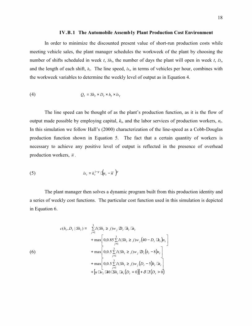
In order to minimize the discounted present value of short-run production costs while

meeting vehicle sales, the plant manager schedules the workweek of the plant by choosing the

number of shifts scheduled in week t, Sht, the number of days the plant will open in week t, Dt,

and the length of each shift, ht. The line speed, lst, in terms of vehicles per hour, combines with

the workweek variables to determine the weekly level of output as in Equation 4.

(4) ttttt lshDShQ ×××=

The line speed can be thought of as the plant’s production function, as it is the flow of

output made possible by employing capital, kt, and the labor services of production workers, nt.

In this simulation we follow Hall’s (2000) characterization of the line-speed as a Cobb-Douglas

production function shown in Equation 5. The fact that a certain quantity of workers is

necessary to achieve any positive level of output is reflected in the presence of overhead

production workers, n .

(5) ( )γγ nnkls ttt −⋅= −1

The plant manager then solves a dynamic program built from this production identity and

a series of weekly cost functions. The particular cost function used in this simulation is depicted

in Equation 6.

(6)

( )

( )

( )( )[ ] ( )0040

5)(5.0,0max

8)(5.0,0max

40)(85.0,0max

)()|,(

1

3

1

3

1

3

1

3

1

>⋅+=⋅⋅⋅⋅+

⋅−∑ ≥+

−∑ ⋅≥+

⋅−∑ ≥+

⋅⋅∑ ⋅≥=

=

=

=

=

tttt

tttj

jt

tttj

jt

tttj

jt

tttj

jtttt

DIDnShwu

nhDwjShI

nhDwjShI

nhDwjShI

nhDwjShIShDhc

δ

19

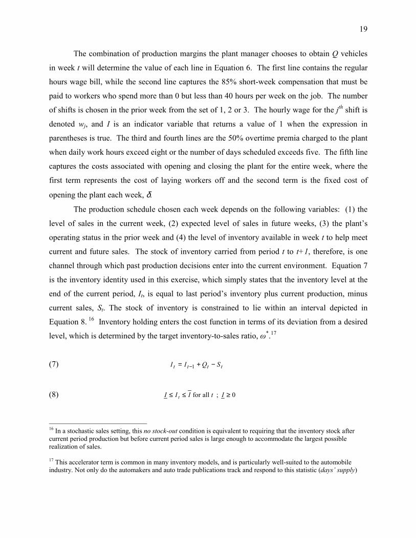
The combination of production margins the plant manager chooses to obtain Q vehicles

in week t will determine the value of each line in Equation 6. The first line contains the regular

hours wage bill, while the second line captures the 85% short-week compensation that must be

paid to workers who spend more than 0 but less than 40 hours per week on the job. The number

of shifts is chosen in the prior week from the set of 1, 2 or 3. The hourly wage for the jth shift is

denoted wj, and I is an indicator variable that returns a value of 1 when the expression in

parentheses is true. The third and fourth lines are the 50% overtime premia charged to the plant

when daily work hours exceed eight or the number of days scheduled exceeds five. The fifth line

captures the costs associated with opening and closing the plant for the entire week, where the

first term represents the cost of laying workers off and the second term is the fixed cost of

opening the plant each week, δ.

The production schedule chosen each week depends on the following variables: (1) the

level of sales in the current week, (2) expected level of sales in future weeks, (3) the plant’s

operating status in the prior week and (4) the level of inventory available in week t to help meet

current and future sales. The stock of inventory carried from period t to t+1, therefore, is one

channel through which past production decisions enter into the current environment. Equation 7

is the inventory identity used in this exercise, which simply states that the inventory level at the

end of the current period, It, is equal to last period’s inventory plus current production, minus

current sales, St. The stock of inventory is constrained to lie within an interval depicted in

Equation 8. 16 Inventory holding enters the cost function in terms of its deviation from a desired

level, which is determined by the target inventory-to-sales ratio, ω*.17

(7) tttt SQII −+= −1

(8) 0 ; allfor ≥≤≤ ItIII t

16 In a stochastic sales setting, this no stock-out condition is equivalent to requiring that the inventory stock aftercurrent period production but before current period sales is large enough to accommodate the largest possiblerealization of sales.

17 This accelerator term is common in many inventory models, and is particularly well-suited to the automobileindustry. Not only do the automakers and auto trade publications track and respond to this statistic (days’ supply)

20

The second channel through which the plant’s history affects current decisions involves

the fixed adjustment costs the plant incurs when the production schedule is changed. Bresnahan

and Ramey (1994) present evidence that changing the line speed or the number of shifts working

entails high adjustment costs, while changing other margins, such as scheduling overtime hours

and closing the plant for week-long intervals, involves relatively low adjustment costs. In our

exercise, changing the number of shifts entails a fixed adjustment cost, αSh.

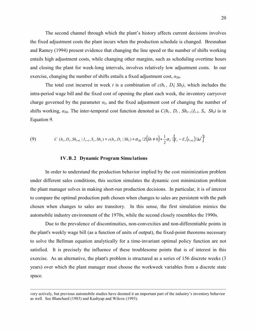
The total cost incurred in week t is a combination of c(ht , Dt| Sht), which includes the

intra-period wage bill and the fixed cost of opening the plant each week, the inventory carryover

charge governed by the parameter αI, and the fixed adjustment cost of changing the number of

shifts working, αSh. The inter-temporal cost function denoted as C(ht , Dt , Sht+1|It-1, St, Sht) is in

Equation 9.

(9) ( ) ( )[ ]2*111 2

10)|,(),,|,,( ωαα ⋅−⋅+≠⋅+= +−+ tttIShttttttttt sEIhSIShDhcShSIShDhC �

IV.B.2 Dynamic Program Simu lations

In order to understand the production behavior implied by the cost minimization problem

under different sales conditions, this section simulates the dynamic cost minimization problem

the plant manager solves in making short-run production decisions. In particular, it is of interest

to compare the optimal production path chosen when changes to sales are persistent with the path

chosen when changes to sales are transitory. In this sense, the first simulation mimics the

automobile industry environment of the 1970s, while the second closely resembles the 1990s.

Due to the prevalence of discontinuities, non-convexities and non-differentiable points in

the plant's weekly wage bill (as a function of units of output), the fixed-point theorems necessary

to solve the Bellman equation analytically for a time-invariant optimal policy function are not

satisfied. It is precisely the influence of these troublesome points that is of interest in this

exercise. As an alternative, the plant's problem is structured as a series of 156 discrete weeks (3

years) over which the plant manager must choose the workweek variables from a discrete state

space.

very actively, but previous automobile studies have deemed it an important part of the industry’s inventory behavioras well. See Blanchard (1983) and Kashyap and Wilcox (1993).

21

To make the dynamic program tractable for numerical solution, the decision variables are

limited to the number of shifts hired for the next week, Sht+1, the number of days open in the

current week, Dt, and the hours scheduled per shift per day, ht. The grids that define the possible

values for each of these choice variables allow the plant manager a reasonable degree of

flexibility in planning the workweek of the plant, but still maintain a state-space of reasonable

dimension for a grid-search solution.18 In particular, it is possible to schedule overtime either

through opening the plant for a sixth day or by scheduling the shift length to exceed 8 hours.

Inventory adjustments can take the form of either a shift reduction or a weeklong plant closure.

A short week is also available through many combinations of production margins.

The line speed in each period is taken as exogenous and is not a choice variable in this

exercise. One can think of line speed as a long-run margin, whose optimal value is determined

by the encompassing profit-maximization problem the auto manufacturer has previously solved

when it designed the plant and chose the type of vehicles it would produce in the current model

year. The set of decision variables in this exercise then determine the workweek of the plant,

given the plant’s configuration and a realized path of sales.19

Sales evolve as a first-order Markov process, where the realization in any given period

may take one of nine possible values. Restricting the realizations of sales to a grid of modest

size is necessary if sales are to be stochastically determined in a grid-search solution algorithm.

The inventory grid consists of points compatible with the sales grid and the production

possibilities, and its boundaries range from a fourteen days’ supply to a ninety days’ supply of

the mean sales rate. The nine sales grid points along with the Markov transition-probability

matrix χ( s’ | s ) are parameterized to mimic a desired AR(1) sales process using Tauchen’s

(1986) procedure. The unconditional mean of sales, µS, is set to the number of vehicles produced

on two shifts using regular-time hours, and thus both scenarios represent a plant that has

correctly matched its full-time capacity with the mean sales rate. Mismatches between the

18 Shifts may take the value of 1, 2 or 3. Days open per week are chosen from the integers 0 through 6. Hours perday are available in increments of 2 ranging from 0 through 10.

19 Taking sales as given in the cost minimization problem does not imply that sales are exogenous to the firm.Rather, we are using a standard micro result that allows us to focus on only the cost minimization part of the overallprofit maximization problem. Automakers often use vehicle-specific incentives to boost weak sales, however it isthe assembly plants’ objective to keep dealers stocked with vehicles in demand, and their relationship becomesstrained when the company promotes unavailable vehicles.

22

capacity of a plant and its realized mean sales are also very important in the determination of

production volatility, and the implications of such occurrences are the subject of Hall (2000).

Since the evidence we have presented above indicates that the most pronounced change

to motor vehicle sales between the periods 1967 – 1983 and 1984 – 2003 has been a reduction in

its serial correlation, this exercise consists of two simulations: Simulation #1 solves the plant’s

cost minimization problem with a persistent monthly sales process (AR(1) = 0.85), and

simulation #2 solves the same problem with the AR(1) coefficient reduced to 0.55. These

parameters match the estimated declines in persistence in the aggregate automobile data. To

determine the pure effect of a change in persistence with no overall change in unconditional

variance, we raise the variance of the innovations in the second simulation so that the

unconditional variance of sales is unchanged between simulations. Thus, these simulations give

a lower bound on how much of the relative change in output volatility we can explain.

The parameter values used throughout this exercise come from the labor contracts

between automakers and their union, parameterizations of assembly plant cost functions from

previous studies (notably Hall (2000)), and from the relatively stable inventory-to-sales ratio

measured in industry data. Parameters that are more difficult to discern, such as the fixed cost of

changing shifts and the marginal cost of deviating from desired inventories, were chosen so that

the solution to the high-persistence version of the model mimics the production behavior

observed among assembly plants in the 1972 – 1983 period as closely as possible.20 21

The sequence of decisions and the arrival of information are as follows: At the beginning

of week t, the plant receives its sales orders for week t, after which the managers schedule the

workweek by choosing values for Dt and ht as well as Sht+1 subject to the relevant constraints.

The orders are then filled and the new level of inventory is carried forward into the next period.

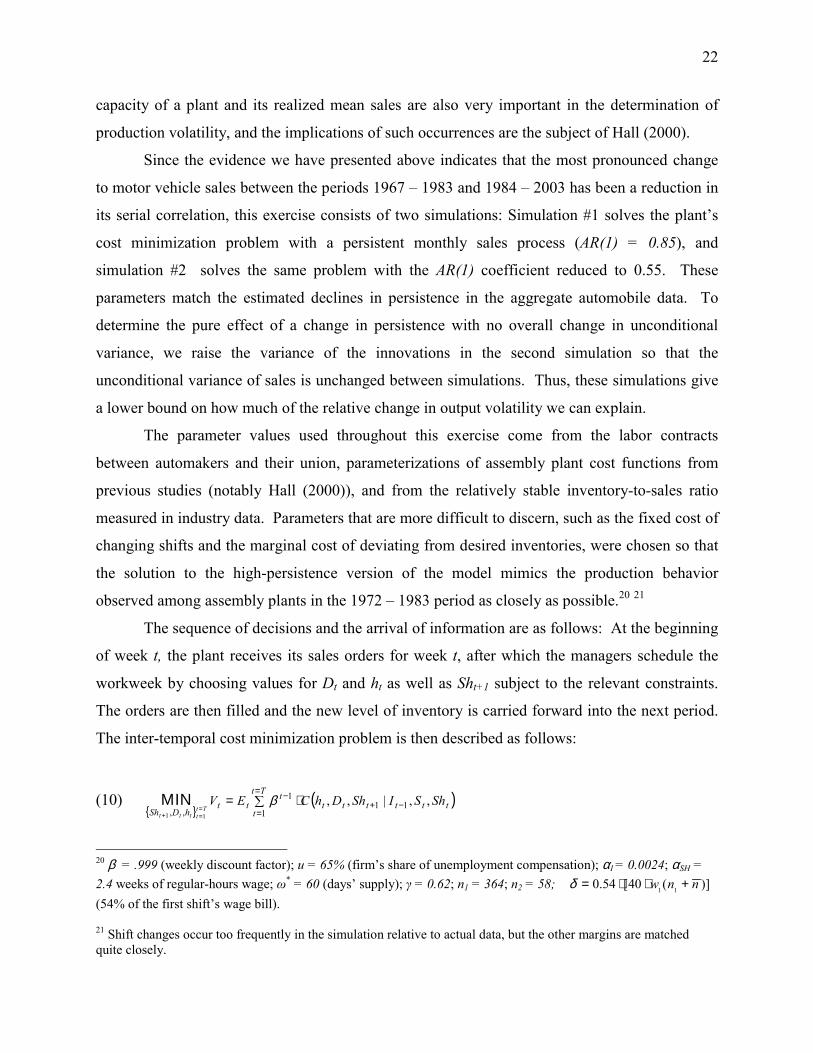
The inter-temporal cost minimization problem is then described as follows:

(10){ }

( )∑ ⋅==

=−+

−==+

ΜΙΝTt

ttttttt

ttt

hDShShSIShDhCEV

Tttttt 1

111

,,,,|,,

11

β

20 β = .999 (weekly discount factor); u = 65% (firm’s share of unemployment compensation); αI = 0.0024; αSH =2.4 weeks of regular-hours wage; ω* = 60 (days’ supply); γ = 0.62; n1 = 364; n2 = 58; 1 10.54 [40 ( )]w n nδ = ⋅ ⋅ +(54% of the first shift’s wage bill).

21 Shift changes occur too frequently in the simulation relative to actual data, but the other margins are matchedquite closely.

23

where ( )tttttt ShSIShDhC ,,|,, 11 −+ is defined as in Equation 9. The solution is subject to the

constraints:

[ ]1 for all 0,

t t tQ S I t T

−≥ − ∈

[ ]T0, allfor ∈≤≤ tIII t ,

where Qt is defined as in Equation 4, and the evolution of final sales

[ ]1

1 1 1| ( | )t

t t t t t ts

E S S S S Sχ+

+ + += ⋅∑

and the initial inventory level

SI µω ⋅= *0 .

The dynamic program is then solved backwards with value functions. 1000 different

paths of sales shocks are generated with a length of 3 years, and in each case the realizations of

sales are constructed for both the persistent (AR(1) = .85) and the more transitory (AR(1) = .55)

sales scenarios.22 The plant solves its weekly cost minimization problem, which determines the

optimal paths for the workweek variables as well as for production and inventory stock. These

solution paths are then aggregated from a weekly to a monthly frequency and their volatility

properties investigated.

The simulation results are summarized in Table 6, which also includes 95% confidence

intervals for certain point estimates and for the changes in the point estimates between scenarios.

In both the high persistence case and in the low persistence (but higher innovation variance)

case, the average (unconditional) standard deviation of monthly sales across simulations is

27.0% of the mean sales rate. The average standard deviation of the optimal production path,

however, changes significantly between the two scenarios. The standard deviation of production

22 The Markov process that generates weekly sales was calibrated so that, on average, monthly sales exhibited thedesired first-order autocorrelation.

24

falls from 40.5% of the mean sales rate per month in the first simulation to 28.0% in the second

simulation. While the average volatility of sales remains unchanged by design between the first

and second simulations, the volatility of production falls. Accordingly, the ratio of the variance

of production over the variance of sales falls from 2.39 to 1.07.

The simulations also generate a change in the covariance of inventory investment and

sales. As Table 6 shows, when sales have a persistence parameter of 0.85, the correlation

between inventory investment and sales is 0.34. In contrast, when sales have a persistence

parameter of 0.55, the correlation becomes -0.15. The intuition is the same as in the standard

production smoothing models of inventory investment. If a sales shock is thought to be very

persistent, then the firm increases its production dramatically in order to maintain its desired

inventory-sales ratio, since it knows sales are likely to stay high for awhile. In contrast, if the

shock is more transitory, the firm is willing to allow a deviation from the desired inventory-sales

ratio since it expects the deviation to be short-lived.

In order to assess from which workweek variables the change in volatility behavior

originates, Table 7 shows the weekly frequency with which various changes to production were

made. Weeklong shutdowns for inventory adjustment, for example, occur in 10.5% of the weeks

when a shock to sales has a persistent effect, and that figure declines just slightly to 9.7% when

the persistence is reduced. Shift reductions, alternatively, are much more common when the

persistence of sales is high. Shift changes occur in 3.8% of the weeks in the high persistence

case, and only in 0.1% of the weeks in the low persistence case. The frequency of the use of

overtime hours, on the other hand, increases from 14.3% in the high persistence scenario to

21.3% in the low persistence simulation. Short-weeks in both scenarios are non-existent.

The conclusion of this simulation exercise is that the variance of output and the

covariance of inventory investment and sales are highly impacted by the nature of the sales

process. When changes in sales are believed to be persistent, the plant often responds by adding

and paring shifts. Alternatively, when changes in sales are transitory, the plant is more likely to

respond with temporary and smaller measures, such as scheduling overtime hours. Thus, if a

given change in the variance of sales stems from a reduction in the persistence of the shocks to

sales, this can lead to a large decline in the variance of output relative to sales. The result is

reached in a simplified production model with certain non-convex costs, but it features no

25

changes to the cost function parameters, inventory targets or improvements in the flow of future

sales information.

The next section investigates changes in production scheduling that have actually taken

place at domestic assembly plants. The changes observed in plant-level data line up quite well

with the model’s predictions.

V. Evidence on Production Scheduling from Plant-Level Data

Our hypothesis states that the change in the nature of the sales process is decreasing the

need to use the non-convex margins that contribute so much to the volatility of production. A

particularly illuminating example of this change is found in Figure 5, which plots weekly posted

production in physical units at Ford’s St. Louis, MO assembly plant during 1972 – 1983 in the

upper panel, and during 1990 – 2001 in the lower panel.23 A feature common to both eras is the

relatively high frequency of weeks where output is zero, which illustrates the intermittent

production behavior discussed above. In addition to shutdowns, however, Ford eliminated the

night shift on two occasions in the early period – once between 1974 and 1976, and then again

between 1980 and 1982. In the late period, the St. Louis assembly plant ran two shifts the entire

time and maintained stable line speeds near 50 vehicles per hour in all model years but 1995.

Weekly production in the late period often exceeds the 4000 vehicles produced on two regular

shifts, however, and the source is the frequent use of daily and weekend overtime hours.

In order to measure changes in production behavior more generally among all Big Three

assembly plants between the 1970s and 1990s, we construct a dataset from industry trade

publications that report production behavior at U.S. and Canadian assembly plants on a weekly

basis over the two time periods: 1972 – 1983 and 1990 – 2001. Bresnahan and Ramey (1994)

collected the data covering the 50 domestic car assembly plants operating in the period 1972 –

1983, and this data set has been significantly extended to include all 103 car and light truck

assembly plants operating within the two periods listed above.24 25

23 Posted production can differ from actual production in instances of unreported deviations from line speed andunreported overtime hours. These are not an important source of volatility, as described by Bresnahan and Ramey(1994).

24 The period 1984 to 1989 was excluded only because we did not have access to Automotive News from that periodwhen we were collecting the data.

26

The data set was collected by reading the weekly production articles in Automotive News,

which report the following variables for all domestic assembly plants: (1) the number of regular

hours the plant works; (2) the number of scheduled overtime hours; (3) the number of shifts

operating; and (4) the number of days per week the plant is closed for (a) union holidays, (b)

inventory adjustments, (c) supply disruptions, and (d) model changeovers. Observations on the

line speed posted on each assembly line were collected from the Wards Automotive Yearbook.26

Table 8 examines how often each margin of production (i.e. plant closures, changes in

shift length, the number of shifts working and line speed) was manipulated during the two

periods. The frequency of margin use among all 103 assembly plants is summarized as a

weighted average, based on each plant’s contribution to total production during the period

examined. Several comparisons between the periods are noteworthy. First, plants shut down at

roughly the same frequency in both periods. The weeklong closures are of particular interest, as

these include the inventory adjustments and model changeovers that directly relate to production

decisions. The frequency of weeklong shutdowns drops from 12.4% in the early period to 11.1%

in the late period, though once holidays are excluded the size of the fall is enhanced somewhat.

Second, the frequency of weeks in which at least four hours of overtime are scheduled has more

than doubled between the periods, rising from 14.4% to 30.3%. Finally, while changes in the

line speed occur with roughly the same frequency in both periods, changes in the number of

shifts occur in 0.6% of the weeks in the early sample, and occur in only 0.1% of the weeks in the

late sample. This implies that the average assembly plant either adds or pares a shift 3.75 times

during the early period, but does so less than once (0.626 times) in the late period.

Table 9 further isolates the plant shutdown margin in the early and in the late periods to

distinguish occurrences that are production planning decisions from those that arise as a

consequence of holidays, the end of the model year, and supply shocks. It shows the percent of

days closed by reason across all plants that were not mothballed, on extended closure, or

permanently removed from service. Thus it considers only temporary closures as opposed to exit

and entry. Inventory adjustments and model changeovers each close plants for a fewer number

25 Data for AMC car plants prior to 1983 were not available, and certain heavy-truck and specialty vehicle facilitieswere excluded, such as the AMC General military vehicle plant, and GMAD Truck & Coach in Pontiac, MI, whichprimarily produces buses.

26 See Bresnahan and Ramey (1994) for more detail about how data is extracted from the weekly production articles.

27

of days in the late period than in the early period, though the decrease in inventory adjustments is

very minor. The number of holidays has increased, and the frequency of supply disruptions,

such as union strikes, parts shortages and natural disasters, is relatively unchanged.

The drop in the average downtime for model changeovers from 4.3 to 2.3 percent of days

is particularly interesting, as this is the margin through which improvements in manufacturing

technology would be visible. There is indeed evidence that model changeover technology has

advanced over time, as the industry introduced the weekend model changeover in the 1970s and

the rolling model changeover in the 1990s. However, the primary means of managing

inventories in the automobile industry, the inventory adjustment, has not changed much despite

the advances in information technology.

The interpretation of these results comes with several caveats. First, the distinction

between inventory adjustments, model changeovers and holidays become blurred during the

winter and summer quarters. Extended Christmas holidays often mask inventory adjustments,27

and model changeovers often take place during a summer vacation or are much longer than the

technology necessitates during periods with low demand.28

When the frequency of production margin use rises and falls, the impact this has on

output volatility depends on the nature of each margin. For example, overtime hours boost

weekly production by up to 25%, while adding a second shift doubles weekly production. Table

10 complements the frequency of use figures by measuring the importance of each production

margin for the variance of output in the pre-1984 and post-1984 periods. To do this analysis, we

construct an artificial output measure, holding each margin constant at some base level. We

determine the impact of a margin on the variance of output by calculating the difference in the

variance of actual output and constructed output. The numbers do not add to 100 because of

nonlinearities and covariance terms.29

Table 10 displays three noticeable changes over the two periods. First, model

changeovers contribute less to the variance of output during the second period. Their impact on

27 Christmas 1982 lasted until almost February 1983 in many plants!

28 An interesting extension of this analysis could evaluate the role of model changeovers in production varianceduring different stages of the business cycle instead of over two discrete pieces of time as we have done. Thiswould be similar to the Cooper and Haltiwanger (1993) study of machine replacement.

29 See Bresnahan and Ramey (1994) for a more detailed explanation of the method.

28

variance falls from 31.1% to 20.3%. Second, the use of overtime hours contributes more than

twice as much to the variance in the second period as it did during the first period, climbing from

a 5.8% contribution to a 13.7% contribution. Third, changes to the number of shifts at individual

plants contribute half as much during the second period as they do during the first period, falling

in contribution from 24.3% to 12.4%.

Thus, the two non-convex margins that lead to so much variance of output – model

changeovers and shifts – are a less important component of the variance of output in the second

period than in the first. Furthermore, overtime hours, which are the classic convex margin of

adjusting production, are more than twice as important during the second period than during the

first. This increase in overtime hours is corroborated by the BLS data on overtime use in the

automobile industry as well, which show a significant increase in overtime used from the early

period to the later period.

VI. Relevance for the Aggregate Economy

The analysis presented here indicates that the persistence of motor vehicle sales has

declined significantly in the post-1984 period, and that this decline can explain observed changes

in the relative volatilities of output and sales as well as the covariance of sales with inventory

investment. Naturally the question arises as to whether this phenomenon is unique to the

automobile industry, or whether it also occurred in the other sectors of the economy that

experienced declines in output volatility.

At first glance it seems that changes to the autocorrelation of sales are unique to the

automobile industry. Blanchard and Simon (2001), Ahmed, Levin and Wilson (2002), and Stock

and Watson (2002) are among those who have tested numerous macroeconomic variables,

including sales, for structural breaks in their autoregressive parameters and have found none.

The motor vehicle sales data used in this study offer two advantages over the sales data used in

these other listed studies, however. First, the frequency of observation is higher – monthly

instead of quarterly; and second, motor vehicle sales are directly measured in physical units

rather than as a chain-weighted index.

These advantages are important to our results, and we believe that the literature’s failure

to find significant changes in sales persistence may owe to data limitations. Plant-level decisions

29

typically occur at the weekly or monthly frequency, so the appropriate sales data would also be

high frequency. Also, production volatility most likely depends on the properties of sales in

physical units as opposed to the properties of their value. These alternative measures of sales, it

turns out, can have very different persistence properties. The reason is that sales measured in

chained-dollars reflect the real expenditures per unit along with its physical-unit quantities. As

shown below for automobiles, real average expenditures per car is a time-series with very high

persistence, and this overwhelms any change in the dynamic properties of unit sales.

Table 11 examines how these two data features (the frequency of observation and the unit

of account) affect the tests for a change in persistence. We estimate the model given in Equation

2, which allows a change in 1984 in the first-order autocorrelation as well as in the conditional

mean and variance, for motor vehicle sales data constructed at different frequencies and with

different units of account. The first three rows replicate changes in the monthly physical unit

sales process measured in Table 4 for cars, light trucks, and their aggregate. In all three cases

there is a significant change in persistence, and in two of three cases there is no significant

change in the variance of the error term.

Consider next the lower panel of Table 11, which inter-temporally aggregates the

physical unit data from the upper panel to a quarterly frequency using averages. In all cases the

changes in the persistence parameter are much smaller in magnitude and are no longer

significant. The changes in the variance of the innovations, on the other hand, now become

significant in each of these series. Monthly data imply a change in the autocorrelation of sales

and no change in the innovation variance, whereas the quarterly data imply just the opposite!

The final row of Table 11 tests the final sales of domestic product of motor vehicles for

changes in persistence and innovation variance. This series is most similar to the types of

variables others have used in more aggregated studies, and it is observed quarterly in units of

chained 1996 dollars.30 The estimated decline in persistence is even smaller in this case than it

was when measured with quarterly physical units in the preceding line, and the change is not

significant. The variance of the innovations, however, appears to have increased significantly in

the second period. Thus, this variable gives answers that are even farther from those obtained

using our preferred data.

30 This variable includes exports. As noted in an earlier section, though, including exports in sales does not changethe estimates noticeably when physical unit data are used.

30

The chained-dollar data contains another element that may be masking the change in

persistence: the behavior of average real expenditures for cars. Chained-dollar sales consist of

the number of physical units multiplied by chained dollar average expenditure per unit. As the

addendum at the bottom of Table 11 shows, average real expenditures per car show no break in

persistence or variance. Average real unit expenditures, however, have a high persistence (first-

order autocorrelation is 0.94), so their effect on chained dollar total expenditures likely hide any

persistence changes in the unit data.31

These exercises suggest that testing for change in sales persistence using standard chain-

weighted quarterly data is not revealing. While general interest in the decline in macroeconomic

volatility focuses on quarterly U.S. GDP growth, it is possible that the true source of this change

is detectable only at higher frequencies and with less aggregation where unit-valued data are

available and meaningful. Thus, the correct data to use in order to verify that the results given

here do or do not extend to other industries are high frequency physical unit data, which we

intend to pursue as future research.

At this point, we offer indirect evidence supportive of the relevance of our hypothesis for

the economy overall. Both the simulations and plant-level data show that when sales persistence

declined in the automobile industry, firms were more likely to vary hours per worker (e.g.

overtime hours) than the number of workers (e.g. the number of shifts). Varying the hours per

worker typically has a low adjustment cost but a high marginal cost, whereas varying the number

of workers has a high adjustment cost but lower marginal cost. Thus, firms will use hours per

worker to respond to transitory shocks and will use employment to respond to more persistent

shocks.

To determine whether production decisions in the overall economy appear to have

changed in the same way as in the automobile industry, we analyze the change in the variances

of the intensive margin (hours per worker) and the extensive margin (number of workers) over

the two periods. The variables used are average weekly hours per worker and the number of

employees in the nonfarm private sector (divided by the population aged 16 and over) at the

31 The case for using physical unit data rather than chained value data can also be made by analogy to studies of thelabor market. One always studies employment variables measured in physical units – either hours or number ofworkers. The stylized facts about labor markets would probably change significantly if economists only studied thereal value of total hours (i.e. the product of real wages and hours) because the high persistence of real wages wouldhide the time series properties of the hours variables.

31

monthly frequency. The product of the two variables is total hours per capita worked in the

nonfarm private sector. We study the growth rates of the variables over the period for which all

of the data are available, which is 1964 to the present.

As Table 12 shows, the variance of total hours fell substantially from the pre-1984 period

to the post-1984 period. Fluctuations in the average hours per employee accounted for 49 percent

of the variance of total hours in the early period but 64 percent of the variance in the later period.

Meanwhile, changes in employment became a smaller part of the overall variance in the second

period. The covariance also declined substantially.

The aggregate labor data display patterns similar to those found in the automobile

industry. The use of margins of adjustment is entirely consistent with the theory that the sales

shocks faced by individual firms in the early period had a higher persistence than those faced by

firms in the later period.

VII. Conclusions

The overview of the automobile industry and analysis conducted using plant-level data

has highlighted several interesting facts that should serve to increase our understanding of the

decline in the variance of GDP. The automobile industry experienced declines in production

volatility around the same time as the rest of the economy. The declines in the automobile

industry were even more dramatic than the declines overall. At least in the case of cars, the

variance of production declined more than the variance of sales.

We presented evidence that the change in production volatility may be linked to changes

in the sales process. We found that changes in the process driving sales appear to be an

important part of the changes in the automobile industry. In contrast to the 1970s and early

1980s, a time when volatile and highly persistent movements in sales beset the automobile

industry, the 1990s featured more transient shocks to sales. We then showed how a change in

the persistence of the sales shocks could lead to a proportionately larger decline in production

volatility over sales volatility.

Plant-level evidence indicates that firms have responded to these changes in the sales

process by reducing their use of non-convex lumpy margins, such as shift changes, and have

32

begun to use the classic convex margin of overtime hours much more intensively. It is likely that

this induced switch is a prime cause of the sharp decline in production volatility.

The brief investigation of the source of the change in the sales process suggests that

monetary policy could be the key. This interpretation is consistent with Clarida Gali and Gertler

(2000), Boivin and Giannoni (2003), and McCarthy and Zakrajšek (2003), all of who find

changes in the estimated monetary policy function at the Federal Reserve to underlie declines in

the persistence of demand shocks and reduced output volatility.

Finally, an analysis of the data suggests that previous failures to find changes in the

persistence of sales at the aggregate level may be due to temporal aggregation and other features

of chain-weighted quantity indexes. Evidence from the aggregate labor market suggests that

firms have varied their labor input in a way that is consistent with sales shocks becoming more

transitory.

33

Data Appendix

Table 1: All data are from the BEA’s NIPA accounts, downloaded November 2003. The data

are in chained 1996 dollars. At the time of writing this paper, the revised accounts with chained

2000 dollars were not available for the durable good and motor vehicle sub-components.

Table 2: All data for car production, inventories and sales are from the BEA. Non seasonally

adjusted truck production is from Wards (extracted from the Federal Reserve’s US database).

Non seasonally adjusted inventory stocks and dealer sales of trucks from 1967 to 1983 are from

volumes of the Wards Automotive Yearbook. The same data for 1984 to 2003 are from the

MVMA (extracted from the Federal Reserve’s US database). The truck production data are

seasonally adjusted using FRB seasonal factors. The truck sales data are seasonally adjusted

using BEA seasonal factors. Car and truck inventory investment series are seasonally adjusted

by regressing them on current and one lag of the relevant production and sales seasonal factors

since the government’s seasonal adjustment factors for inventories do not extend back very far.

Table 3: All series are from the BEA.

Table 4: Division-level sales data are from Wards Communications. We include dummy

variables for each month in which sales are affected by a strike, as well as the month afterward.

The set of dummy variables include the following months: 1967:9 – 1968:1, 1970:9 - 1971:1,

1976:10 - 1976:12. Although most strikes only affect one company, we included the full set of

dummy variables for each company and division to capture spillover effects.

Table 5: The real price of cars is the CPI for new cars divided by the overall CPI. No truck CPI

is available, so we use the CPI for new motor vehicles for both light trucks and motor vehicles

overall. Income is from the BEA and the Federal Funds rate is from the Federal Reserve Board

of Governors.

Tables 8–10: As discussed in the text, all data were collected by hand from articles in

Automotive News.

Table 11: The additional chain-weighted data are from the BEA.

Table 12: Data from the BLS.

34

References

Aizcorbe, A., "Experience Rating, Layoffs and Unions: A Look at U.S. Assembly PlantLayoffs," Manuscript, Bureau of Labor Statistics, 1990

Aizcorbe, A., "Procyclical Labour Productivity, Increasing Returns to Labour and LabourHoarding in Car Assembly Plant Employment," Economic Journal, 102, 1992, 860 – 873.

Ahmed, S., Levin, A. and Wilson, B. A., "Recent U.S. Macroeconomic Stability: Good Policies,Good Practices, or Good Luck?" The Board of Governors of the Federal Reserve System,July 2002.

Automotive News, Detroit: Crain Automotive Group.

Blanchard, O. J., "The Production and Inventory Behavior of the American AutomobileIndustry," The Journal of Political Economy, 91(3), June 1983, 365 – 400.

Blanchard, O.J. and Simon, J., “The Long and Large Decline in U.S. Output Volatility,”Brookings Papers on Economic Activity, 2001:1, 135 – 164.

Boivin, J. and Giannoni, M.P., “Has Monetary Policy Become More Effective?” NBER WorkingPaper Series #9459, January 2003.

Bresnahan, T. F. and Ramey, V. A., “Segment Shifts and Capacity Utilization in the U.S.Automobile Industry,” American Economic Review Papers and Proceedings, 83(2), May 1993,213 – 218.

-----------------------, "Output Fluctuations at the Plant Level," The Quarterly Journal ofEconomics, August 1994, 593 – 624.

Clarida, R., Galí, J., and Gertler, M., “Monetary Policy Rules and Macroeconomic Stability:Evidence and some Theory,” Quarterly Journal of Economics, 115, February 2000, 147 –180.

Cooper, R. and Haltiwanger, J., “The Aggregate Implications of Machine Replacement: Theoryand Evidence,” American Economic Review, 83(3), June 1993, 360 – 382.

-----------------------, “Automobiles and the National Industrial Recovery Act: Evidence onIndustry Complementarities,” Quarterly Journal of Economics 108(4), November 1993,1043 – 1072.

Feroli, M., “An Equilibrium Model of Inventories with Investment-Specific Technical Change,”Working paper, New York University, November 2002.

35

Golob, J. E., "Post-1984 Inventories Revitalize the Production-Smoothing Model," WorkingPaper, University of Missouri - Kansas City, 2000.

Hall, G. J., "Non-convex Costs and Capital Utilization: A Study of Production Scheduling atAutomobile Assembly Plants," Journal of Monetary Economics, 45 (2000), 681 – 716.

Hetrick, R.L., “Analyzing the Recent upward Surge in Overtime Hours,” Monthly Labor Review,February 2000, 30 – 33.

Irvine, O. and Schuh, S., “Inventory Investment and Output Volatility,” Working paper, FederalReserve Bank of Boston, December 2002.

Kahn, J.A., “Why is Production More Volatile than Sales? Theory and Evidence on theStockout-Avoidance Motive for Inventory-Holding,” Quarterly Journal of Economics,107, May 1992, 481 – 510.

Kahn, J. A., McConnell, M. M. and Perez-Quiros, G., "On the Causes of the Increased Stabilityof the U.S. Economy," FRBNY Economic Policy Review, May 2002, 183 – 202.

Kashyap, A.K. and Wilcox, D.W., “Production and Inventory Control at the General MotorsCorporation During the 1920’s and 1930’s,” American Economic Review 83(3), June1993, 383 – 401.

Kim, C. and Nelson, C. R., "Has the U.S. Economy Become More Stable? A Bayesian ApproachBased on a Markov-Switching Model of the Business Cycle," The Review of Economicsand Statistics, 81(4), November 1999, 608 – 616.

Kim, C., Nelson, C.R., and Piger, J., “The Less Volatile U.S. Economy: A BayesianInvestigation of Timing, Breadth and Potential Explanations,” Federal Reserve Board ofGovernors, International Finance Discussion Paper 707, August 2001.

McConnell, M.M., and Perez-Quiros, G., "Output Fluctuations in the United States: What hasChanged Since the Early 1980s?" American Economic Review, 90(5), December 2000,1464 – 76.

McCarthy, J. and Zakrajšek, E., “Inventory Dynamics and Business Cycles: What hasChanged?” Finance and Economics Discussion Series, Federal Reserve Board ofGovernors, June 2003.

Ramey, V. A., "Nonconvex Costs and the Behavior of Inventories," Journal of PoliticalEconomy, 99, 1991, 306 – 334.

Ramey, V. A. and Vine, D. J., “Why Do Real and Nominal Inventory-Sales Ratios HaveDifferent Trends?” forthcoming Journal of Money, Credit and Banking.

36

Ramey, V. A. and Vine, D. J., “The Effect of Sales Persistence on Volatility in a ProductionSmoothing Model,” 2003b, manuscript.

Ramey, V. A. and West, K. D., "Inventories," in Handbook of Macroeconomics, eds. John D.Taylor and Michael Woodford, Elsevier Science Press.

Stock, J.H. and Watson, M.W., “Has the Business Cycle Changed and Why?” NBER WorkingPaper Series #9127, September 2002.

-----------------------, “Understanding Changes in International Business Cycle Dynamics,” NBERWorking Paper Series #9859, July 2003a.

-----------------------, “Has the Business Cycle Changed? Evidence and Explanations,” August2003b.

Tauchen, G., “Finite State Markov-Chain Approximations to Univariate and VectorAutoregressions,” Economics Letters, 20(1986), 177 – 181.

Wards Automotive Yearbook, Detroit: Wards Communications.

Warnock, M. and Warnock, F., “The Declining Volatility of U.S. Employment: Was ArthurBurns Right?” Federal Reserve Board of Governors, International Finance DiscussionPaper 677, August 2000

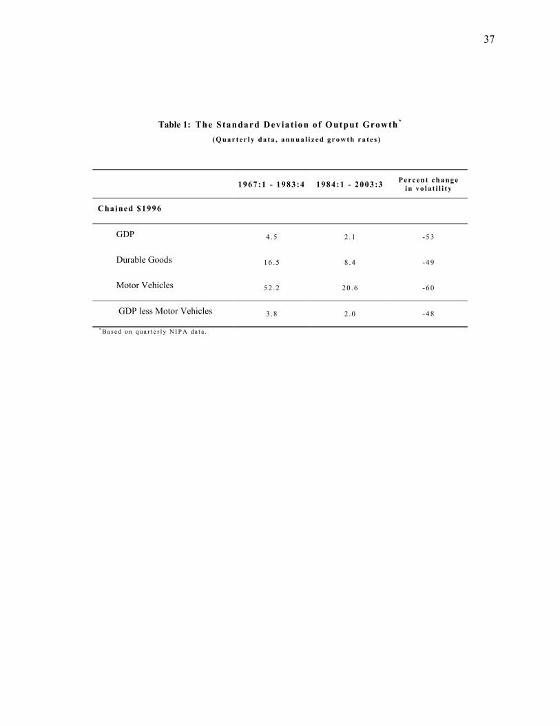
37

Table 1: The Standard Deviat ion of Output Growth *

(Qua r ter ly da ta , ann ua l i zed grow th ra te s )

1967:1 - 1983:4 1984:1 - 2003:3 Percent changei n vo l a t i l i ty

Chained $1996

GDP 4.5 2 .1 -5 3

Durable Goods 16 .5 8 .4 -4 9

Motor Vehicles 5 2 . 2 2 0 . 6 -6 0

GDP less Motor Vehicles 3 .8 2 .0 -4 8

* B a s e d o n q ua r t e r l y N I P A d a t a .

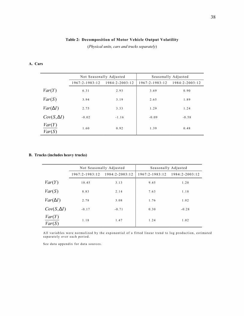
38

Table 2: Decomposition of Motor Vehicle Output Volatility

(Physical units, cars and trucks separately)

A. Cars

Not Season al ly Adju s t ed Seasonal ly Adjus t ed

1967:2-1983:12 1984:2-2003:12 1967:2-1983:12 1984:2-2003:12

( )Var Y 6 . 3 1 2 . 9 3 3 . 6 9 0 . 9 0

( )Var S 3 . 9 4 3 . 1 9 2 . 6 5 1 . 8 9

( )Var I∆ 2 . 7 5 3 . 3 3 1 . 2 9 1 . 2 4

( , )Cov S I∆ -0 . 0 2 -1 . 1 6 -0 . 0 9 -0 . 5 8

( )( )

Var YVar S

1 . 6 0 0 . 9 2 1 . 3 9 0 . 4 8

B. Trucks (includes heavy trucks)

Not Season al ly Adju s t ed Seasonal ly Adjus t ed

1967:2-1983:12 1984:2-2003:12 1967:2-1983:12 1984:2-2003:12

( )Var Y 1 0 . 4 5 3 . 1 3 9 . 4 5 1 . 2 0

( )Var S 8 . 8 3 2 . 1 4 7 . 6 3 1 . 1 8

( )Var I∆ 2 . 7 8 3 . 0 8 1 . 7 6 1 . 0 2

( , )Cov S I∆ -0 . 1 7 -0 . 7 1 0 . 3 0 -0 . 2 8

( )( )

Var YVar S

1 . 1 8 1 . 4 7 1 . 2 4 1 . 0 2

Al l va r i a b l es we r e n o rma l i z ed b y t h e exp on en t i a l o f a f i t t ed l i n ea r t r en d t o l og p rod u c t i on , es t i ma t edsep a ra t e l y o v er ea c h p e r i od .

See d a t a a p p en d i x f or d a t a sou rc es .

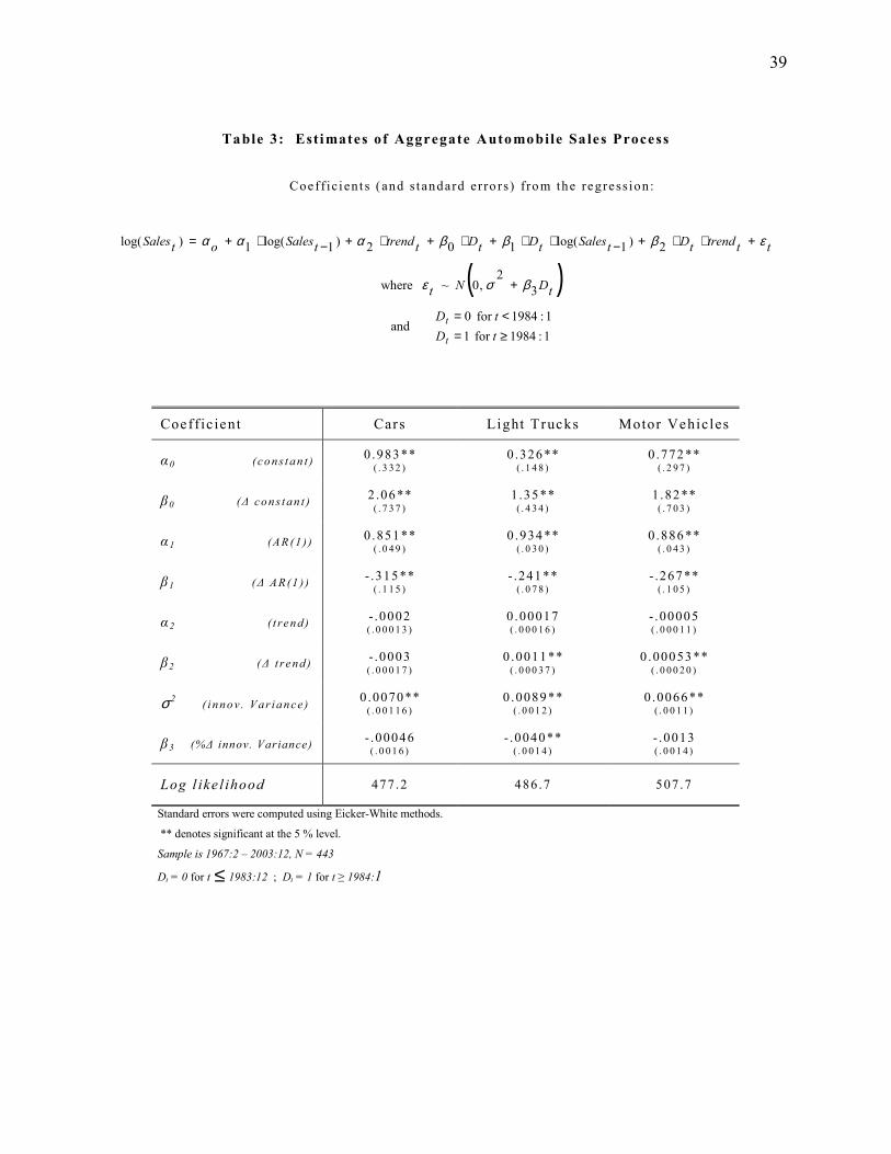
39

Table 3: Est imates of Aggregate Automobile Sa les Process

Coeff ic i en t s ( and s t andard er ro rs) fro m the regress ion :

tttrendtDtSalestDtDttrendtSalesotSales εβββααα +⋅⋅+−⋅⋅+⋅+⋅+−⋅+= 2)1log(102)1log(1)log(

where ( )tDNt 32

,0~ βσε +

and 1:1984for 11:1984for 0

≥=<=

tDtD

t

t

Coeffic ient Cars Light Trucks Motor Vehicles

α 0 (co n s t a n t ) 0 .983 **( . 3 3 2 )

0 .326 **( . 1 4 8 )

0 .772 **( . 2 9 7 )

β0 (∆ c o n s t a n t ) 2.06 **( . 7 3 7 )

1 .35 **( . 4 3 4 )

1 .82 **( . 7 0 3 )

α 1 (AR (1 ) ) 0 .851 **( . 0 4 9 )

0 .934 **( . 0 3 0 )

0 .886 **( . 0 4 3 )

β1 (∆ AR(1 ) ) - .315 **( . 1 1 5 )

- .241 **( . 0 7 8 )

- .267 **( . 1 0 5 )

α 2 ( t r en d ) - .0002( . 0 0 0 1 3 )

0 .00017( . 0 0 0 1 6 )

- .00005( . 0 0 0 1 1 )

β2 (∆ t r e n d ) - .0003( . 0 0 0 1 7 )

0 .0011 **( . 0 0 0 3 7 )

0 .00053 **( . 0 0 0 2 0 )

σ2 ( i nnov . Va r i ance ) 0 .0070 **( . 0 0 1 1 6 )

0 .0089 **( . 0 0 1 2 )

0 .0066 **( . 0 0 1 1 )

β3 (%∆ innov. Variance) - .00046( . 0 0 1 6 )

- .0040 **( . 0 0 1 4 )

- .0013( . 0 0 1 4 )

Log l ike l ihood 477.2 486 .7 507 .7

Standard errors were computed using Eicker-White methods.

** denotes significant at the 5 % level.

Sample is 1967:2 – 2003:12, N = 443

Dt = 0 for t ≤ 1983:12 ; Dt = 1 for t ≥ 1984:1

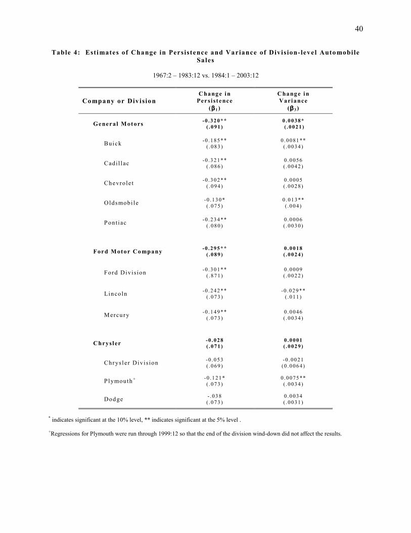
40

Table 4: Est imates of Change in Persistence and Variance of Divis ion-leve l Auto mobi leSales

1967:2 – 1983:12 vs. 1984:1 – 2003:12

Company or Div isionChang e in

Persi st ence(ββββ 1 )

Chang e inVariance

(ββββ 3 )

General Motors -0 . 3 2 0 * *( .0 9 1 )

0 . 0 0 38 * ( . 0 0 2 1 )

Buick -0 . 1 8 5 **( .0 8 3 )

0 . 0 0 81 **( .0 0 3 4 )

Cadi l l ac -0 . 3 2 1 **( .0 8 6 )

0 . 0 0 56( .0 0 4 2 )

Ch evrole t -0 . 3 0 2 **( .0 9 4 )

0 . 0 0 05( .0 0 2 8 )

O ldsmobi le -0 . 1 3 0 *( .0 7 5 )

0 . 0 1 3 **( .0 0 4 )

Pont iac -0 . 2 3 4 **( .0 8 0 )

0 . 0 0 06( .0 0 3 0 )

Ford Motor Co mpany -0 . 2 9 5 * *( .0 8 9 )

0 . 0 0 18( .0 0 2 4 )

Ford Div is ion -0 . 3 0 1 **( .8 7 1 )

0 . 0 0 09( .0 0 2 2 )

Lin coln -0 . 2 4 2 **( .0 7 3 )

-0 . 0 2 9 **( .0 1 1 )

Mercu ry -0 . 1 4 9 **( .0 7 3 )

0 . 0 0 46( .0 0 3 4 )

Chrysl er -0 . 0 2 8( .0 7 1 )

0 . 0 0 01( .0 0 2 9 )

Chrys l er Div is ion -0 . 0 5 3( .0 6 9 )

-0 . 0 0 2 1(0 . 0 0 6 4 )

P lymouth + -0 . 1 2 1 *( .0 7 3 )

0 . 0 0 75 **( .0 0 3 4 )

Dod ge - .0 3 8( .0 7 3 )

0 . 0 0 34( .0 0 3 1 )

* indicates significant at the 10% level, ** indicates significant at the 5% level .

+Regressions for Plymouth were run through 1999:12 so that the end of the division wind-down did not affect the results.

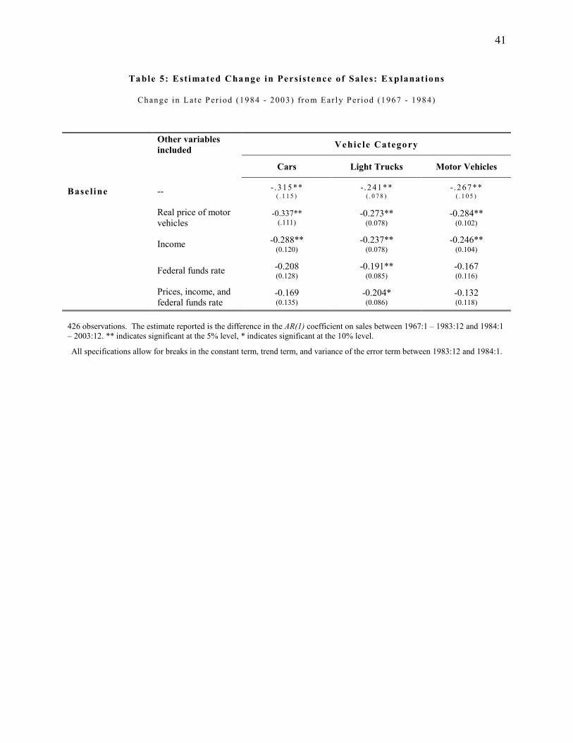
41

Table 5: Est imated Change in Persistence of Sales: Explanat ions

Change in Lat e Per iod (1984 - 2003) fro m Ear ly Per iod (1967 - 1984)

Other variablesincluded Vehic le Category

Cars Light Trucks Motor Vehicles

Base line -- - .315 **( . 1 1 5 )

- .241 **( . 0 7 8 )

- .267 **( . 1 0 5 )

Real price of motorvehicles

-0.337**(.111)

-0.273**(0.078)

-0.284**(0.102)

Income -0.288**(0.120)

-0.237**(0.078)

-0.246**(0.104)

Federal funds rate -0.208(0.128)

-0.191**(0.085)

-0.167(0.116)

Prices, income, andfederal funds rate

-0.169(0.135)

-0.204*(0.086)

-0.132(0.118)

426 observations. The estimate reported is the difference in the AR(1) coefficient on sales between 1967:1 – 1983:12 and 1984:1– 2003:12. ** indicates significant at the 5% level, * indicates significant at the 10% level.

All specifications allow for breaks in the constant term, trend term, and variance of the error term between 1983:12 and 1984:1.

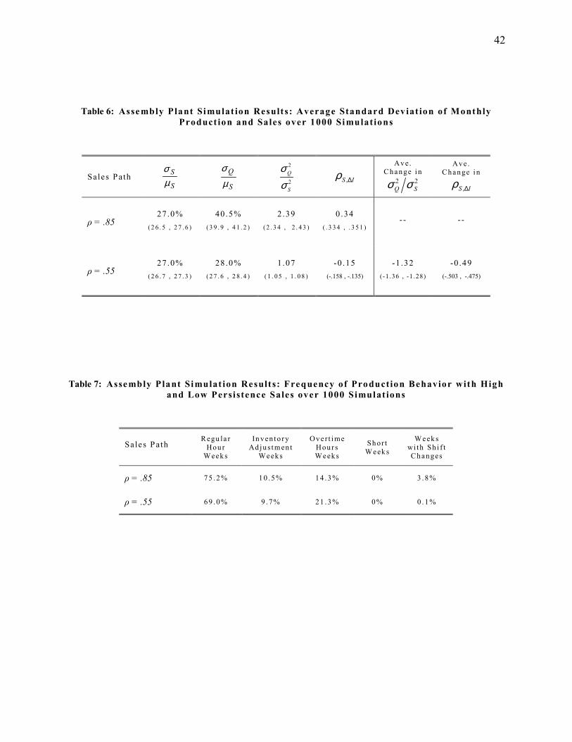
42

Table 6: Assembly Plant Simulat ion Result s: Average Standard Deviat ion of MonthlyProduct ion and Sales over 1000 Simulat ions

Sales PathS

Sµσ

S

Q

µσ 2

2Q

S

σσ ,S Iρ ∆

Av e.Change i n

2 2Q Sσ σ

Av e.Change i n

,S Iρ ∆

ρ = .8527 .0%

( 2 6 . 5 , 2 7 . 6 )

40 .5%( 3 9 . 9 , 4 1 . 2 )

2 .39( 2 . 3 4 , 2 . 4 3 )

0 .34( . 3 3 4 , . 3 5 1 )

- - - -

ρ = .5527 .0%

( 2 6 . 7 , 2 7 . 3 )

28 .0%( 2 7 . 6 , 2 8 . 4 )

1 .07( 1 . 0 5 , 1 . 0 8 )

-0 .15(-.158 , -.135)

-1 .32(-1.36 , -1 .28)

-0 .49(-.503 , -.475)

Table 7: Assembly Plant Simulat ion Result s: Frequency of Production Behavior with Highand Low Persistence Sales over 1000 Simulat ions

Sales PathRegu la r

Hou rWeek s

In v en t o r yAd j u s t m en t

Week s

Ov e r t imeHou r sWeek s

Sh or tWeek s

Week swi t h Sh i f tC h a n ges

ρ = .85 7 5 . 2 % 1 0 . 5 % 1 4 . 3 % 0 % 3 . 8 %

ρ = .55 6 9 . 0 % 9 . 7 % 2 1 . 3 % 0 % 0 . 1 %

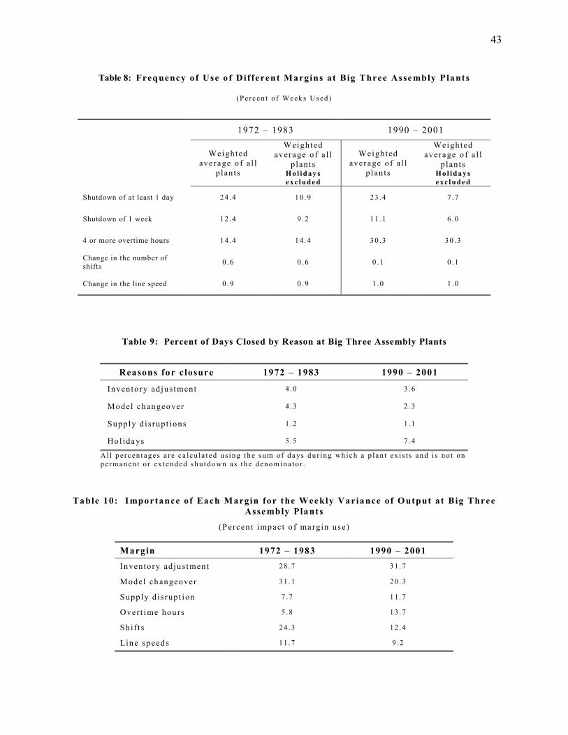
43

Table 8: Frequency of Use o f Different Margins at Big Three Assembly Plants

(P erc en t o f Week s Us ed )

1972 – 1983 1990 – 2001

Weightedaverage o f a l l

p lan ts

Weightedaverage o f a l l

p lan tsHo l i da y sexc lude d

Weightedaverage o f a l l

p lan ts

Weightedaverage o f a l l

p lan tsHo l i da y sexc lude d

Shutdown of at least 1 day 2 4 .4 1 0 .9 2 3 .4 7 .7

Shutdown of 1 week 1 2 .4 9 .2 1 1 .1 6 .0

4 or more overtime hours 1 4 . 4 1 4 . 4 3 0 . 3 3 0 . 3

Change in the number ofshifts 0 .6 0 .6 0 .1 0 .1

Change in the line speed 0 .9 0 .9 1 .0 1 .0

Table 9: Percent of Days Closed by Reason at Big Three Assembly Plants

Reasons for c losure 1972 – 1983 1990 – 2001

Inventory ad ju s tment 4 .0 3 .6

Model ch angeo ver 4 .3 2 .3

Supply d i srup t ions 1 .2 1 .1

Hol idays 5 .5 7 .4

Al l p erc en t a g e s a r e c a lcu la t ed u s i n g t h e su m of d a ys d u r i n g wh i c h a p la n t ex i s t s a n d i s n o t onp erma n en t o r ex t en d ed sh u t d o wn a s t h e d en o mi n a t or .

Table 10: Importance of Each Margin for the Weekly Variance of Output at Big ThreeAssembly Plants

(Percen t imp act o f margin use)

Margin 1972 – 1983 1990 – 2001Inventory ad ju s tment 2 8 . 7 3 1 . 7

Model ch angeo ver 3 1 . 1 2 0 . 3

Supply d i srup t ion 7 . 7 1 1 . 7

Over t ime hours 5 . 8 1 3 . 7

Shi f t s 2 4 . 3 1 2 . 4

Lin e sp eed s 11 .7 9 .2

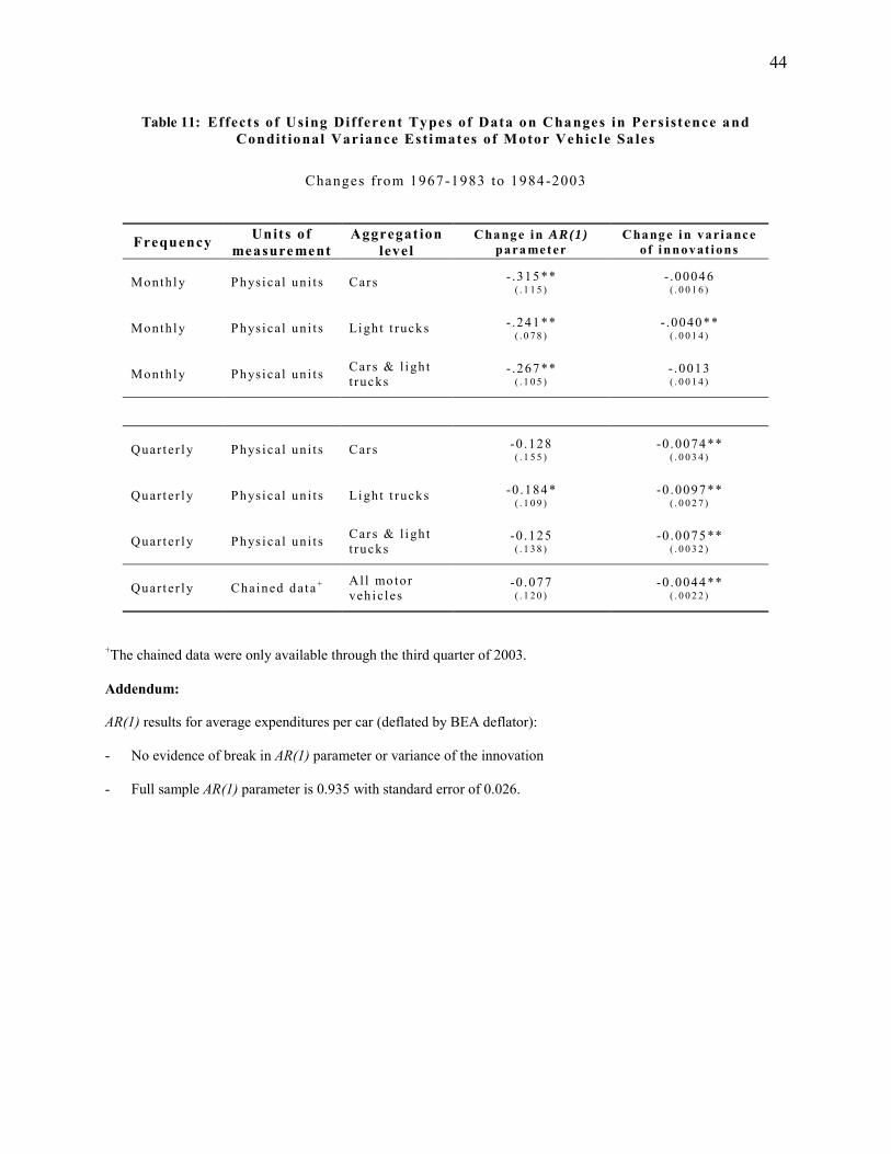
44

Table 11: Effects of Using Different Types of Data on Changes in Pers istence andCondit ional Variance Estimates of Motor Vehic le Sa les

Changes from 1967-1983 to 1984-2003

Frequency Units ofmeasurement

Aggregat ionleve l

Chang e in AR(1)para meter

Chang e in varianceof innovat ions

Monthly Physi cal un i t s Car s - .315 **( . 1 1 5 )

- .00046( . 0 0 1 6 )

Month ly Physi cal un i t s Ligh t t rucks - .241 **( . 0 7 8 )

- .0040 **( . 0 0 1 4 )

Month ly Physi cal un i t s Car s & l i gh tt rucks

- .267 **( . 1 0 5 )

- .0013( . 0 0 1 4 )

Quar t er ly Phys i cal uni t s Car s -0 .128( . 1 5 5 )

-0 .0074 **( . 0 0 3 4 )

Quar t er ly Physi cal un i t s Ligh t t rucks -0 .184 *( . 1 0 9 )

-0 .0097 **( . 0 0 2 7 )

Quar t er ly Phys i cal un i t s Car s & l i gh tt rucks

-0 .125( . 1 3 8 )

-0 .0075 **( . 0 0 3 2 )

Quar t er ly Chained d at a+ Al l mo torveh icl es

-0 .077( . 1 2 0 )

-0 .0044 **( . 0 0 2 2 )

+The chained data were only available through the third quarter of 2003.

Addendum:

AR(1) results for average expenditures per car (deflated by BEA deflator):

- No evidence of break in AR(1) parameter or variance of the innovation

- Full sample AR(1) parameter is 0.935 with standard error of 0.026.

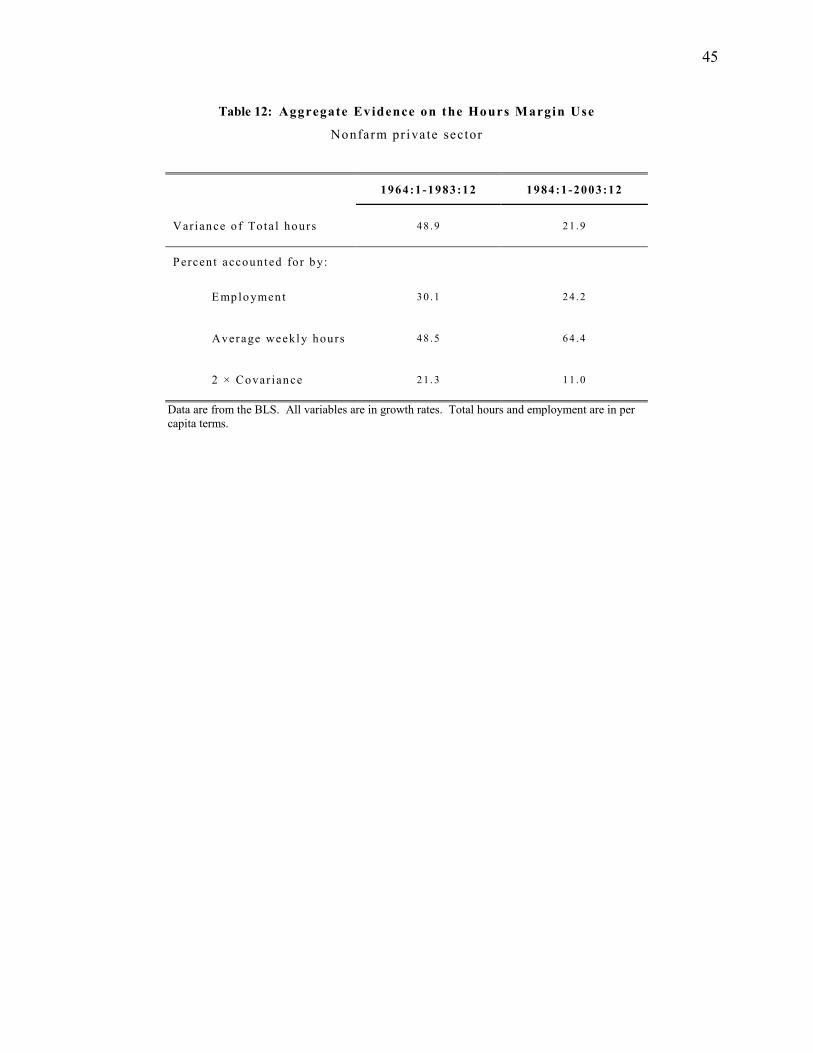
45

Table 12: Aggregate Evidence on the Hours Margin Use

Nonfarm pr iva te sector

1964:1-1983:12 1984:1-2003:12

Varian ce o f Tota l hours 4 8 . 9 2 1 . 9

Percen t accounted fo r b y:

Emp lo ymen t 3 0 . 1 2 4 . 2

Average weekly hours 4 8 . 5 6 4 . 4

2 × Covar ian ce 2 1 . 3 1 1 . 0

Data are from the BLS. All variables are in growth rates. Total hours and employment are in percapita terms.

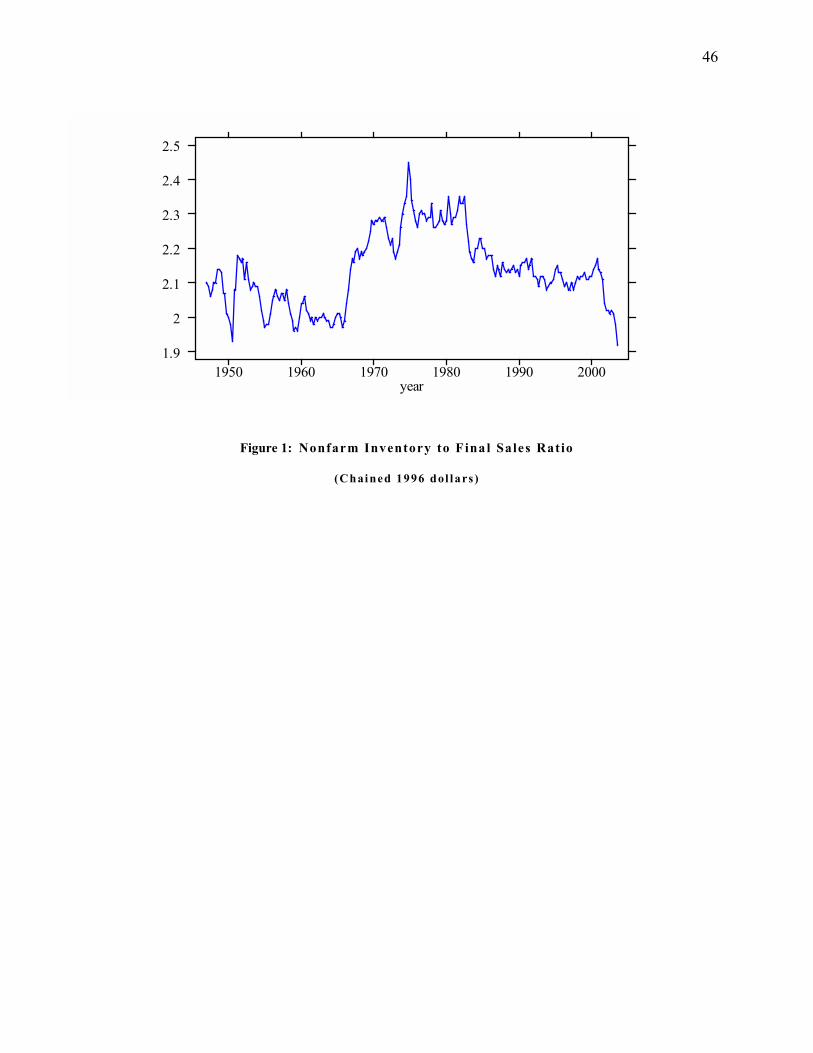
46

Figure 1: Nonfarm Inventory to Fina l Sales Ratio

(Chained 1996 dol lars )

year1950 1960 1970 1980 1990 2000

1.9

2

2.1

2.2

2.3

2.4

2.5

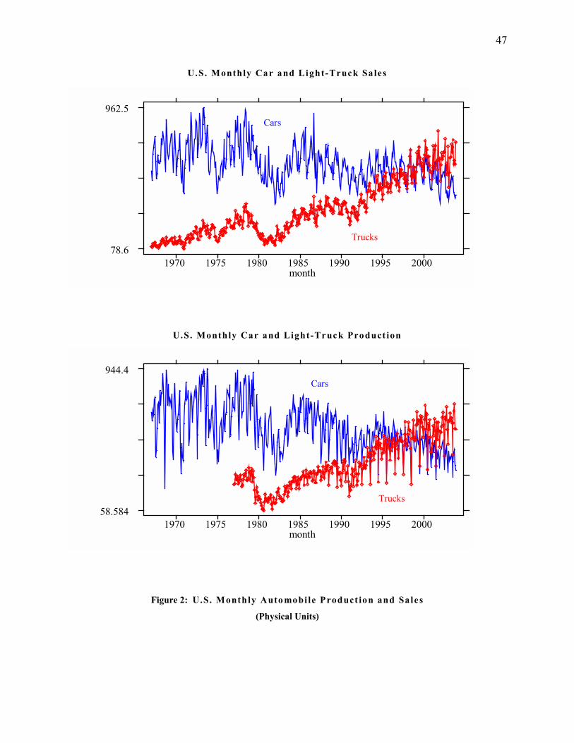
47

U.S. Monthly Car and Light-Truck Sa les

U.S. Monthly Car and Light-Truck Product ion

Figure 2: U.S. Monthly Auto mobi le Product ion and Sales

(Physical Units)

month1970 1975 1980 1985 1990 1995 2000

78.6

962.5Cars

Trucks

month1970 1975 1980 1985 1990 1995 2000

58.584

944.4Cars

Trucks

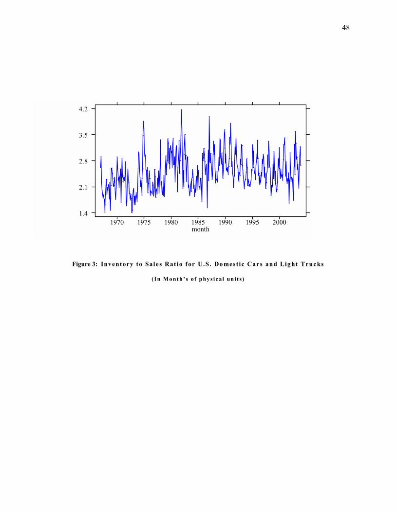
48

Figure 3: Inventory to Sales Rat io for U.S. Do mestic Cars and Light Trucks

(In Month’s of phy si cal uni t s)

month1970 1975 1980 1985 1990 1995 2000

1.4

2.1

2.8

3.5

4.2

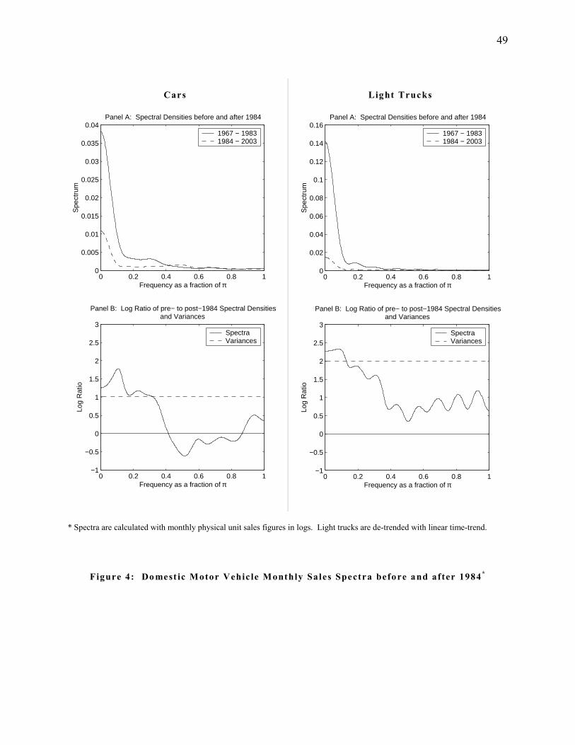
49

Cars

0 0.2 0.4 0.6 0.8 10

0.005

0.01

0.015

0.02

0.025

0.03

0.035

0.04

Frequency as a fraction of π

Spe

ctru

m

Panel A: Spectral Densities before and after 1984

1967 − 19831984 − 2003

0 0.2 0.4 0.6 0.8 1−1

−0.5

0

0.5

1

1.5

2

2.5

3

Frequency as a fraction of π

Log

Rat

io

Panel B: Log Ratio of pre− to post−1984 Spectral Densitiesand Variances

SpectraVariances

Light Trucks

0 0.2 0.4 0.6 0.8 10

0.02

0.04

0.06

0.08

0.1

0.12

0.14

0.16

Frequency as a fraction of π

Spe

ctru

m

Panel A: Spectral Densities before and after 1984

1967 − 19831984 − 2003

0 0.2 0.4 0.6 0.8 1−1

−0.5

0

0.5

1

1.5

2

2.5

3

Frequency as a fraction of π

Log

Rat

ioPanel B: Log Ratio of pre− to post−1984 Spectral Densities

and Variances

SpectraVariances

* Spectra are calculated with monthly physical unit sales figures in logs. Light trucks are de-trended with linear time-trend.

Figure 4: Do mest ic Motor Vehic le Monthly Sales Spectra before and after 1984*

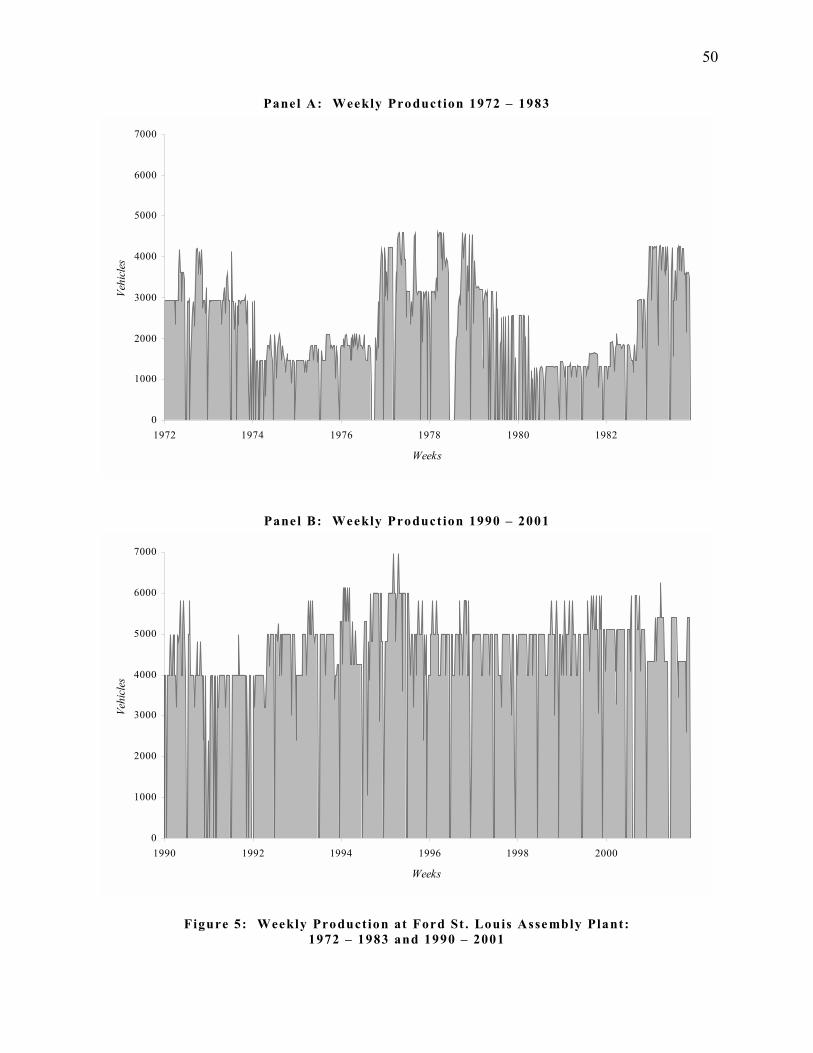
50

Panel A: Weekly Production 1972 – 1983

0

1000

2000

3000

4000

5000

6000

7000

1972 1974 1976 1978 1980 1982

Weeks

Vehi

cles

Panel B: Weekly Product ion 1990 – 2001

0

1000

2000

3000

4000

5000

6000

7000

1990 1992 1994 1996 1998 2000

Weeks

Vehi

cles

Figure 5: Weekly Production at Ford St . Louis Assembly Plant:1972 – 1983 and 1990 – 2001