Tractable Experiment Design via Mathematical Surrogates

Brian Williams LA-UR-16-21255

Statistical Sciences Group, Los Alamos National Laboratory

Abstract This presentation summarizes the development and implementation of quantitative design criteria motivated by targeted inference objectives for identifying new, potentially expensive computational or physical experiments. The first application is concerned with estimating features of quantities of interest arising from complex computational models, such as quantiles or failure probabilities. A sequential strategy is proposed for iterative refinement of the importance distributions used to efficiently sample the uncertain inputs to the computational model. In the second application, effective use of mathematical surrogates is investigated to help alleviate the analytical and numerical intractability often associated with Bayesian experiment design. This approach allows for the incorporation of prior information into the design process without the need for gross simplification of the design criterion. Illustrative examples of both design problems will be presented as an argument for the relevance of these research problems.

Slide 1

Rare Event Estimation •  Interested in rare event estimation

–  Outputs obtained from computational model –  Uncertainties in operating conditions and physics variables –  Physics variables calibrated wrt reference experimental data

•  In particular, quantile or percentile estimation

–  One of qα or α is specified and the other is to be inferred –  qα may be random when inferring α

•  Sequential importance sampling for improved inference –  Oversample region of parameter space producing rare events of

interest –  Sequentially refine importance distributions for improved inference

Slide 2

Pr[ ⇥(x,�) > q� ] = �

Example: VR2plus Model

•  Scenario: Pressurizer failure, followed by pump trip and initiation of SCRAM (insertion of control rods)

•  Goal: Understand behavior of peak coolant temperature (PCT) in the reactor

•  Interested in probability that PCT exceeds 700o K

Slide 3

VR2plus Details •  Single thermal-hydraulics loop with 21 components

•  Working coolant is water at 16MPa and 600o K, single-phase flow

•  Nominal power output of this reactor is 15MW

•  Calculations performed with reactor safety analysis code R7 (INL)

Slide 4

Input Parameter Min Max Description PumpTripPre 15.6 MPa 15.7 MPa Min. pump pressure causing trip PumpStopTime 10 s 100 s Relaxation time of pump phase-out PumpPow 0.0 0.4 Pump end power SCRAMtemp 625o K 635o K Max. temp. causing SCRAM CRinject 0.025 0.24 Position of CR at end of SCRAM CRtime 10 s 50 s Relaxation time of CR system

Input parameters assigned independent Uniform distributions on their ranges

•  Sample from alternative distribution g(x,θ), evaluate computational model, and weight each output

–  Percentile estimator:

–  Quantile estimator: Smallest value of qα for which

•  Importance density g(x,θ) ideally chosen to increase the likelihood of observing desired rare events

Importance Sampling

�1[�(x,�)>q�](x,�) w(x,�)g(x,�) dx d�

w(x,�) � f(x) �(�)g(x,�)Importance weight Importance density

Slide 5

�̂(g) =1N

N�

j=1

w(x(j),�(j)) 1[�(x(j),�(j))>q�](x(j),�(j))

�̂(g) � �

minimum variance importance density g(x,�) =

1�

1[�(x,�)>q�]f(x)⇥(�)

Goal: Approximate minimum variance importance density to achieve substantial variance reduction

•  A subset of variables may be responsible for generating rare events –  Relevant xr, θr

–  Irrelevant xi, θi

•  Minimum variance importance distribution

•  Importance distribution g(x,θ) becomes

Relevant (Sensitive) Variables

Slide 6

�(x,�) = �( (xr, x̃i), (�r, �̃i) ) for all values of x̃i and �̃i

g(x,�) = gr(xr,�r)fi(xi|xr)�i(�i|�r)

gr(xr,�r) =1�

1[�(x,�)>q�](x,�)fr(xr)⇥r(�r) for any values of xi and �i

gi( (xi,�i)|(xr,�r) ) = fi(xi|xr)�i(�i|�r)

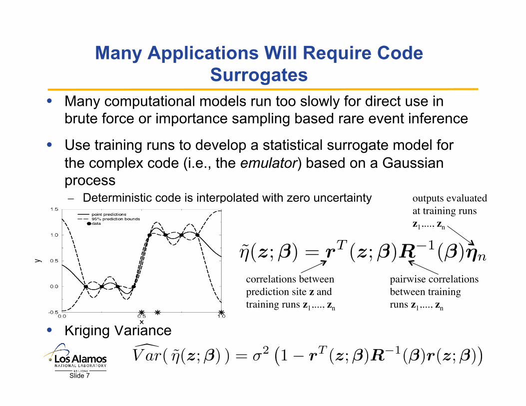
Many Applications Will Require Code Surrogates

•  Many computational models run too slowly for direct use in brute force or importance sampling based rare event inference

•  Use training runs to develop a statistical surrogate model for the complex code (i.e., the emulator) based on a Gaussian process –  Deterministic code is interpolated with zero uncertainty

•  Kriging Predict

•  Kriging Variance

Slide 7

correlations between prediction site z and training runs z1,..., zn

pairwise correlations between training runs z1,..., zn

outputs evaluated at training runs z1,..., zn

⌘̃(z;�) = rT (z;�)R�1(�)⇥n

dV ar( �̃(z;�) ) = ⇥2�1� rT (z;�)R�1(�)r(z;�)

�

Surrogate-based Percentile/Quantile Estimation •  Gaussian Process model with plug-in covariance parameter

estimates, e.g.

•  Process-based inference

Slide 8

Pr [�(x,�) > q|(x,�)] = �

0

@ �̃(x,�)� qqdV ar( �̃(x,�) )

1

A

� =

Z�

0

@ ⇥̃(x,�)� q↵qdV ar( ⇥̃(x,�) )

1

A w(x,�) g(x,�) dx d�

�̂(g) =1

N

NX

j=1

�

0

@ ⇥̃(x(j),�(j))� q�qdV ar( ⇥̃(x(j),�(j)) )

1

A w(x(j),�(j))

�̃(x,�)� �(x,�)qdV ar( �̃(x,�) )

⇠ N(0, 1)

Adaptive Importance Sampling

Slide 9

•  Choose g(x,θ) by iterative refinement 1.  Sample from initial importance density

g(1)(x,θ) = f(x) π(θ) 2.  Given target probability or quantile level, determine which

parameters are sensitive for producing extreme output values

●

●

●

●

●

●

●

●

●●

●●●

●

●

●●●●

●●●

●●●●●●●

●

●

●

●●●●●

●

●

●●

●

●

●

●●●

●

●● ●●●

●●●●

●●

●

●

●

●

●●

●●●

●

●

●●

●

●

●●

●

●●

●

●●

●

●

●●● ●

●

●●

●

●

●

●● ●

● ●

●

0.0 0.1 0.2 0.3 0.4

0.05

0.10

0.15

0.20

Pump Power

Con

trol R

od P

ositi

on

Figure 7: Rare Events at the 700�K (�) level.

34

●

●

●

●

●

●

●

●

●

●

●

●

●

●

●

●

●

●

●

●

●

●

●

●

●

●

●

●

●

●

●

●

●

●

●

●

●

●

●

●

●

●

●

●

●

●

●

●

●

●

●

●

●

●

●

●

●

●

●

●

●

●

●

●●

●

●

●

●

●

●

●

●

●

●●●

●

●

●

●

●

●

●

●

●

●

●

●

●

●●

●

●

●

●

●

●

●●

20 40 60 80 100

1020

3040

50

Pump Stop Time

Con

trol R

od R

elax

atio

n Ti

me

Figure 9: Rare Events at the 700�K (�) level.

36

Adaptive Importance Sampling

Slide 10

3.  For sensitive parameters, adopt a family of importance densities (e.g. Beta, (truncated) Normal, etc.). Fit the parameters of this family to the selected largest order statistics (e.g. method of moments, MLE).

4.  Keep the conditional distribution for the insensitive parameters, given values of the sensitive parameters.

5.  Combine the distributions of (3) and (4) to obtain g(2)

(x,θ). 6.  If applicable, refine the surrogate in the input region of

interest, e.g. using information provided by g(2)(x,θ). 7.  Repeat (2)-(6) until the updated importance

distribution g(k)(x,θ) “stabilizes” in its approximation of the minimum variance importance distribution.

Convergence Assessment Through Iterative Refinement of Surrogate

•  Surrogate bias may affect inference results

•  Choose design augmentation that minimizes integrated mean square error with respect to the currently estimated importance distributions for sensitive parameters –  A version of “targeted” IMSE (tIMSE)

IMSE(Db) = 1�trace

"Zr{D0,Db}(z;�) r

T{D0,Db}(z;�)

nzY

i=1

wi(zi) dz

#R�1

{D0,Db}(�)

!

For sensitive input i, select wi(zi) to be its importance distribution

Estimate correlation parameters based on current design D0

Slide 11

VR2plus Analysis •  Percentile inference

–  PCT > 700o K •  Importance distribution

–  Independent Beta distributions for sensitive parameters –  Independent Uniform distributions for insensitive parameters

Slide 12

●

●

●

●

●

●

●

●

●

●

●

●

●

●

●

●

●

●

●

●

●

●

●

●

●

●

●

●

●

●

●

●

●

●

●

●

●

●

●

●

●

●

●

●

●●

●

●

●●

●●

●

●

●

●●

●

●

●

●

●

●

●

●

●●

●

●

●

●

●

●

●

●

●

●

●

●

●

●

●

●

●

●

●

●

●

●

●

●

●

●

●

●

●●

●●

●

0.000 0.005 0.010 0.015 0.020 0.025 0.030

0.20

0.21

0.22

0.23

0.24

Pump Power

Con

trol R

od P

ositi

on

0.00 0.01 0.02 0.03 0.04 0.05

010

20

30

40

50

60

70

PumpPow

PDF

0.20 0.21 0.22 0.23 0.24

020

40

60

80

CRinject

PDF

Importance Distributions VRF = 42

PumpPow and CRinject are sensitive

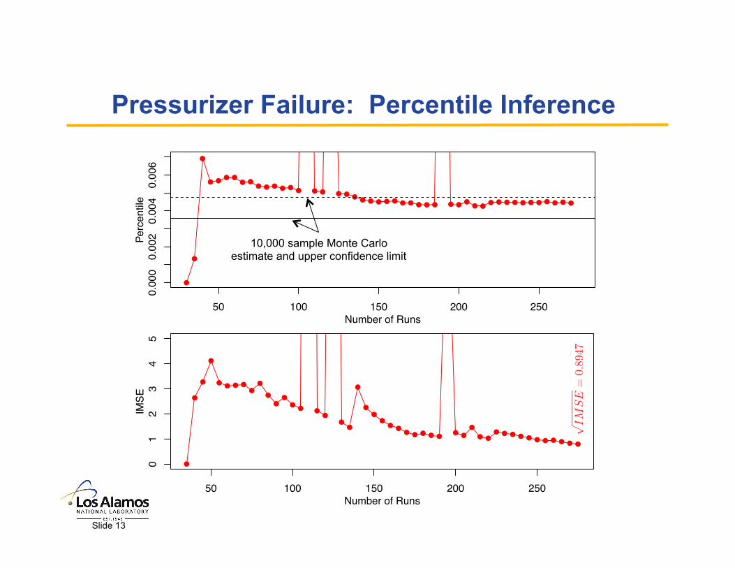
Pressurizer Failure: Percentile Inference

Slide 13

50 100 150 200 250

0.0

00

0.0

02

0.0

04

0.0

06

Number of Runs

Pe

rce

ntile

!

!

!

! !! !

! !! ! ! ! !

! ! ! ! ! !! ! ! ! ! ! ! ! ! ! ! !

!! !

! ! ! ! ! ! ! ! ! ! !

10,000 sample Monte Carlo estimate and upper confidence limit

50 100 150 200 250

01

23

45

Number of Runs

IMS

E

!

!

!

!

!! ! !

!

!

!

!!

!! !

!!

!

!

!

!!

!!

! ! ! ! !! !

!

! !! ! ! ! ! ! ! ! ! ! !

Bayesian Experimental Design

•  Decision-theoretic approach to designing experiments that assimilates the objectives of the experiment with prior information to arrive at an optimal set of new runs

•  Chaloner, K. and Verdinelli, I. (1995) is an excellent review article on Bayesian experimental design

•  Based on utility functions –  Represent preferences: U(x) ≥ U(y) if and only if x is preferred to y

•  Two primary experimental objectives: estimation and prediction

Slide 14

Expected Utility •  Design η must be chosen from some set H •  Data y observed from sample space Y •  Based on y, a decision d is chosen from some set D •  Unknown parameter θ defined on parameter space Θ •  General utility function U(d, θ, η, y)

•  Bayesian experimental design solution η* :

U(⌘) =

Z

Ymax

d2D

Z

⇥U(d, ✓, ⌘,y) p(✓|y, ⌘) p(y|⌘) d✓ dy

U(⌘⇤) = max

⌘2H

Z

Y

max

d2D

Z

⇥U(d, ✓, ⌘,y) p(✓|y, ⌘) p(y|⌘) d✓ dy

p(y, θ | η)

Slide 15

Motivating Application: Accelerated Testing

•  Items will not fail under certain conditions

•  Such items are exposed to accelerated conditions to induce failure

•  Typical application: Estimating the lifetime distribution of reliable items

LANL: Understanding the conditions that induce undesirable explosions Accelerated testing has become commonplace

Slide 16

Motivating Application: Test Planning

•  Key question: How can prior knowledge be incorporated into accelerated test planning?

•  Prior knowledge implemented as an informative prior distribution on model parameters –  Obtained from sequential testing –  Experience with similar populations

•  A test consists of –  Choosing the levels of the accelerators –  Proportion of units at each selected level

Slide 17

0.0050.010.02

0.05

0.1

0.20.30.40.50.60.70.8

0.9

0.95

0.98

100 200 500 1000 2000 5000 10000 2500050000Time

Prop

ortio

n Fa

iling

Temperature Degrees C

406080

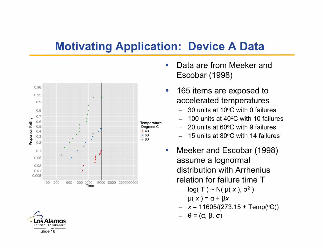
Motivating Application: Device A Data •  Data are from Meeker and

Escobar (1998)

•  165 items are exposed to accelerated temperatures –  30 units at 10oC with 0 failures –  100 units at 40oC with 10 failures –  20 units at 60oC with 9 failures –  15 units at 80oC with 14 failures

•  Meeker and Escobar (1998) assume a lognormal distribution with Arrhenius relation for failure time T –  log( T ) ~ N( µ( x ), σ2 ) –  µ( x ) = α + βx –  x = 11605/(273.15 + Temp(oC)) –  θ = (α, β, σ)

Slide 18

Motivating Application: New Data

•  Suppose –  Different yet similar items to Device A are to be tested next –  Expect a similar failure mechanism as Device A –  Posterior distribution of θ resulting from Device A analysis is

relevant –  Becomes the prior distribution p(θ) for planning and analyzing the next test

•  Notation –  η is an accelerated test

–  Temperatures to test and corresponding proportions –  t is a vector of failure and censoring times corresponding to η –  t0.1 is the 0.1 quantile of the failure-time distribution –  var( t0.1 | t, η, 10oC ) is the posterior variance of t0.1 at 10oC

Slide 19

Motivating Application: Test Constraints

•  Experimentalists specify a temperature range of [10oC,80oC] for new tests –  10oC represents the use condition –  Testing above 80oC will introduce a new failure mechanism not

seen at the use condition

•  All tests end at a censoring time of tc = 5000 hours, independent of test η

•  Interest in estimating t0.1 at 10oC with high precision –  t0.1(x) = exp{ α + βx + σ Φ-1(0.1) }, Φ denotes standard normal CDF –  x = 11605/(273.15 + Temp(oC)) = 11605/(273.15 + 10) ≈ 41 –  Therefore, t0.1 at 10oC is a function t0.1(θ) of parameters θ only

Slide 20

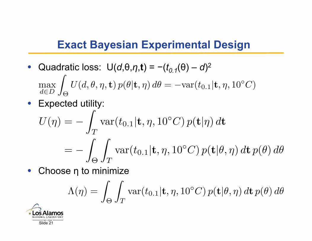
Exact Bayesian Experimental Design

•  Quadratic loss: U(d,θ,η,t) = −(t0.1(θ) – d)2

•  Expected utility:

•  Choose η to minimize

max

d2D

Z

⇥U(d, ✓, ⌘, t) p(✓|t, ⌘) d✓ = �var(t0.1|t, ⌘, 10�C)

U(⌘) = �Z

Tvar(t0.1|t, ⌘, 10�C) p(t|⌘) dt

= �Z

⇥

Z

Tvar(t0.1|t, ⌘, 10�C) p(t|✓, ⌘) dt p(✓) d✓

⇤(⌘) =

Z

⇥

Z

Tvar(t0.1|t, ⌘, 10�C) p(t|✓, ⌘) dt p(✓) d✓

Slide 21

Design Criterion Estimation

•  Given η, Λ(η) is estimated as follows: 1.  Draw θ* from p(θ) 2.  Simulate lifetimes t* from their lognormal sampling distribution

given θ* and η 3.  Censor the elements of t* exceeding tc 4.  Using importance sampling or MCMC to generate a posterior

sample of θ given t* and η, estimate var( t0.1(θ) | t*, η, 10oC ) and denote the resulting sample variance by V*(η)

5.  Repeat steps 1-4 to obtain for J large (e.g. J = 10,000)

6.  Compute the Monte Carlo estimate

V ⇤1 (⌘), . . . , V

⇤J (⌘)

⇤̂(⌘) =1

J

JX

j=1

V ⇤j (⌘)

⇤(⌘) =

Z

⇥

Z

Tvar(t0.1|t, ⌘, 10�C) p(t|✓, ⌘) dt p(✓) d✓

Slide 22

Using GPs to Estimate Optimal Designs 1.  Select a set of initial designs η1, η2, …, ηk and compute

design criterion estimates –  Initial designs are generated, for example, via random or Latin

hypercube sampling

2.  Fit a GP to

3.  Apply the Expected Quantile Improvement (EQI) algorithm with this GP to select the next design ηk+1.

–  EQI selects a design that minimizes an upper quantile of Λ(η).

4.  Increment k to k+1

5.  Repeat steps 2-4 until run budget expires or EQI stopping criteria are satisfied.

⇤̂(⌘1), ⇤̂(⌘2), . . . , ⇤̂(⌘k)

⇤̂k = [⇤̂(⌘1), ⇤̂(⌘2), . . . , ⇤̂(⌘k)]

Slide 23

Motivating Application: EQI Implementation

•  Design η has the following form

•  Zhang, Y. and Meeker, W.Q. (2006) suggests a near-optimal test will have B = 2 –  Our search restricted to this case, so that GP is a function of the 3

inputs (Temp1, Temp2, π1):

⌘ =

2

6664

Temp1 ⇡1

Temp2 ⇡2.

.

.

.

.

.

TempB ⇡B

3

7775where ⇡i � 0 for i = 1, . . . , B and

BX

i=1

⇡i = 1

⌘ =

Temp1 ⇡1

Temp2 1� ⇡1

�

Slide 24

0 20 40 60 80 1002000

025

000

3000

035

000

4000

0

0

20

40

60

80

100

Temperature 1

Tem

pera

ture

2

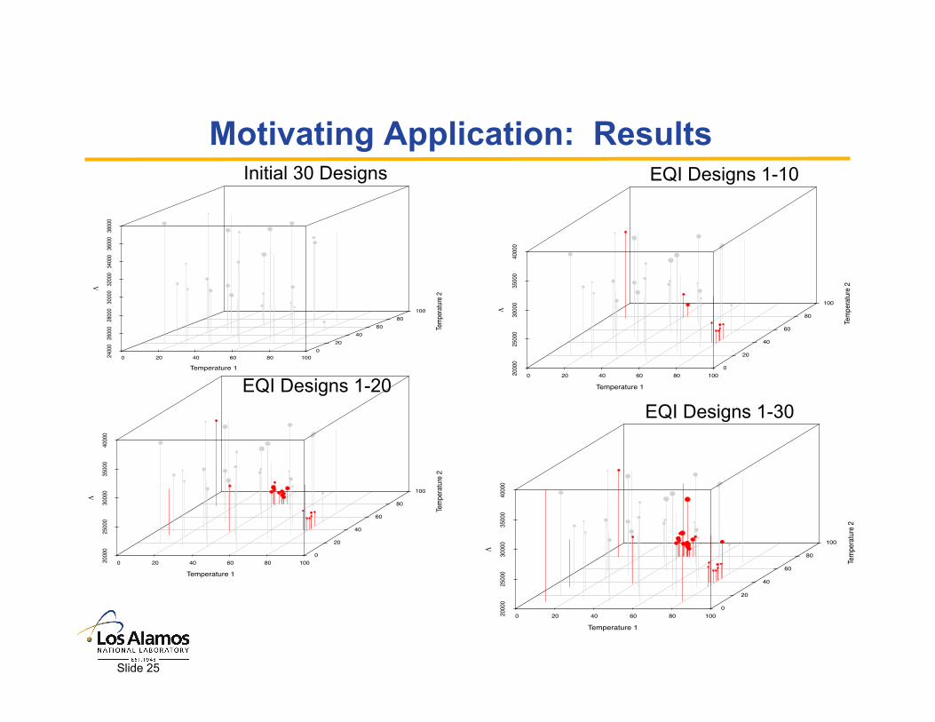
Λ

EQI Designs 1-20

Motivating Application: Results

0 20 40 60 80 1002400

026

000

2800

030

000

3200

034

000

3600

038

000

0 20

40 60

80100

Temperature 1

Temp

eratur

e 2

Λ

Initial 30 Designs

0 20 40 60 80 1002000

025

000

3000

035

000

4000

0

0

20

40

60

80

100

Temperature 1

Tem

pera

ture

2

Λ

EQI Designs 1-10

0 20 40 60 80 1002000

025

000

3000

035

000

4000

0

0

20

40

60

80

100

Temperature 1

Temp

eratu

re 2

Λ

EQI Designs 1-30

Slide 25

Motivating Application: Comparisons

0 20 40 60 80 1002000

025

000

3000

035

000

4000

0

0

20

40

60

80

100

Temperature 1Te

mpe

ratu

re 2

Λ

Exact Bayes: EQI Iterates Approximate Bayes: MLE & Device A posterior for p(θ)

Reduce censoring time so that posterior is not approximately Gaussian: Exact Bayes: EQI Iterates EQI Optimal Design Approximate Bayes

Slide 26

Conclusions

Slide 27

•  Surrogates enable optimization of computationally intensive experimental design criteria –  Slow running codes –  Analytically intractable criterion functions

•  Percentile and quantile estimation –  Importance sampling improves UQ of percentile and quantile

estimates relative to brute force approach –  Sequential design improves surrogate quality in region of

parameter space indicated by importance distributions

•  Bayesian experimental design –  Powerful framework for incorporating prior information into optimal

designs –  Estimation of analytically intractable design criteria can be

mitigated through the application of surrogate-based optimization techniques