Trade and Foreign Direct Investment in China:

A Political Economy Approach

by

Lee G. BranstetterDept. of Economics, Univ. of California, Davis

and NBER

and

Robert C. FeenstraDept. of Economics, Univ. of California, Davis,

Haas School of Business, Univ. of California, Berkeley,and NBER

Revised, March 1999

Acknowledgements: We thank Chen Chun-Lai, Wen Hai, David Li, Barry Naughton, DanielRosen, Scott Rozelle, Edward Steinfeld, William Skinner, Eric Thun, Shang-Jin Wei, WingWoo, Alwyn Young and seminar participants at the University of Michigan and the World Bankfor helpful comments and suggestions. We are indebted to a large team of research assistants,including Natasha Hsieh, Songhua Lin, Kaoru Nabeshima, Shun-li Yao, and David Yue.Branstetter wishes to thank the Japan Foundation Center for Global Partnership and the SocialScience Research Council for financial support of the fieldwork component of this project, andhe thanks the many anonymous China-based multinational executives who provided theirinsights concerning the environment confronting foreign firms in China. He also acknowledgesthe support of a University of California Faculty Research Grant. Feenstra thanks the NationalScience Foundation for financial support. All errors are the sole responsibility of the authors.

Trade and Foreign Direct Investment in China:

A Political Economy Approach

Abstract

We view the political process in China as trading off the social benefits of increased trade

and foreign direct investment, against the losses incurred by state-owned enterprises due to such

liberalization. A model drawing on Grossman and Helpman (1994, 1996) is used to derive an

empirically estimable government objective function. The key structural parameters of this

model are estimated using province-level data on foreign direct investment and trade flows in

China, over the years 1984-1995. We find that the weight applied to consumer welfare is

between one-fifth and one-twelfth of the weight applied to the output of state-owned enterprises.

We find that governmental preferences have shifted over time, but even in recent periods the

weight on consumer welfare is only one-half of the weight on state-owned enterprises. This

suggests that China may find it politically difficult to follow through with liberalizing its trade

and investment regimes, such as under its WTO accession proposal.

Lee Branstetter Robert FeenstraDepartment of Economics Department of EconomicsUniversity of California University of CaliforniaDavis, CA 95616 Davis, CA 9561(530)752-3033 (530)752-7022branstet@ucdavis.edu rcfeenstra@ucdavis.edu

1

1. Introduction

In recent years, few developments in international economics have elicited more interest

or stirred more controversy than the sudden emergence of China as a trading nation and

manufacturing center.1 China’s high rate of economic growth since the adoption of more liberal

economic policies under Deng Xiao-Ping in the late 1970s, while perhaps exaggerated by the

official statistics, is nevertheless a stunning accomplishment.2 In the space of less than a

generation, China has transformed itself from a poor nation almost completely cut off from the

global economy to one of the world’s most important suppliers of labor-intensive manufactures.

Its arrival into the ranks of trading nations will be complete when it is has achieved its intention

to join the World Trading Organization (WTO).

Nevertheless, a number of economists have recently called into question the sustainability

of China’s current rates of GDP and export growth. These observers have tended to point out the

shortcomings of China’s “socialist market economy,” focusing on the inability of the

government to raise revenue by taxing the new private economy, the problems the government

has encountered in reforming state owned enterprises, the distortions created by China’s dualistic

trade regime, and the mounting “non performing loans” problem in the Chinese banking sector.3

In a striking paper, Alwyn Young (1997) has recently argued that China’s high trade/GDP ratio

is a sign of intra-national trade barriers rather than international economic openness. Particularly

since the onset of the East Asian financial crisis, the consensus has shifted to a more pessimistic

outlook for China.

The reality of important distortions in the Chinese economy, and particularly in its

international trade regime, is increasingly evident. We offer, in this paper, what is to our

1 For an excellent overview of this emergence, see Naughton (1996).

2

knowledge the first attempt to use the theoretical models of political economy pioneered by

Grossman and Helpman (1994) to analyze these distortions. We view the political process in

China as trading off the social benefits of increased trade and foreign direct investment, against

the losses incurred by state-owned enterprises due to such liberalization. We write down an

explicit theoretical model of the policy formulation process which, we argue, captures important

features of Chinese institutional reality. We then use this model to derive an empirically

estimable governmental objective function. The key structural parameters of this model are

estimated using province-level data on foreign direct investment and trade flows in China in the

years 1984-1995.

These estimates allow us to quantify the relative weights placed on “special interests” and

general economic welfare. In striking contrast to Goldberg and Maggi’s (1997) results with U.S.

data, we find quantitative evidence that Chinese provincial and central governments have given

much greater weight to the special interests of state-owned enterprises than to general economic

welfare. Moreover, our empirical framework allows us to estimate how the weights in the

government’s objective function have shifted over time. In other words, we can quantify the

extent to which Chinese political economy has become more “market-oriented” over the course

of the reform period. Finally, our framework allows us to estimate the impact on governmental

utility of proposed changes in China’s trade regime. As an experiment, we estimate the impact

of the tariff reductions China has offered as part of its bid for WTO accession. The implications

of these findings for the political economy literature and for the debate over economic reform in

China are discussed in the conclusion. The proofs of propositions are gathered in a separate

Appendix.

2 See Sachs and Woo (1997) for a discussion with some reference to the problems of official Chinese statistics.3 Again, Naughton (1996) provides an excellent overview of these issues.

3

2. Policies towards Foreign Direct Investment and Trade

A comprehensive description of Chinese economic reform, even one focused solely on

the evolution of China’s trade and FDI regime, is well beyond the scope of this paper. The

reader is directed to Lardy (1992) and Naughton (1995) for two well-regarded studies.4 Here, we

quickly summarize some of the most important policy shifts that directly relate to FDI and trade.

The formal ban on foreign direct investment in China was lifted in 1972, in the wake of

the visit of U.S. President Richard Nixon to China. This opened the doors for a diplomatic

rapprochement between China and several major industrial nations. However, a number of

severe restrictions on FDI remained in place – including a ban on external financing of FDI

projects – so that there was very little inward investment until policies were dramatically

changed in 1979.

By 1979, Deng Xiao-Ping had consolidated his power within the Chinese government

and the Communist Party. At his behest, a new Law on Joint Ventures was passed, providing a

basic framework under which foreign firms were allowed to operate. Restrictions on external

debt and equity finance were relaxed, and controls on foreign trade were reduced. Provincial and

local governments were allowed considerable freedom in regulating the joint ventures that were

established within their jurisdictions. In the same year, four “special economic zones” (SEZ)

were established in which foreign firms were offered preferential tax and administrative

treatment, and given an unusually free hand in their operations.5 In particular, these zones

charged a reduced tax of 15% on business income of foreign affiliated firms (as compared to

33% for domestic firms), but these taxes were not levied during the first two years of operation

4 The material in this section also draws on Grub and Lin (1991) and Pomfret (1991).5 These SEZs included Shenzhen (across the border from Hong Kong), Zhuhai (across the border from Macau),Shantou (on the Guangdong coast facing Taiwan) and Xiamen (directly across the Taiwan Straits from Taiwan).

4

and charged at one-half of the full rate in the third through fifth years.6 In addition, wholly

foreign owned enterprises were permitted for the first time. It is important to recognize that none

of the original special economic zones were developed industrial centers in 1979. In fact, these

zones were established outside the state’s industrial centers to prevent “contamination” of

Chinese heavy industry by outside influences. These “experiments” in attracting foreign direct

investment were quite successful. In 1984, fourteen additional areas known as “open coastal

cities”, were granted similar exemptions from taxes and administrative procedures in a bid to

attract FDI.7 These cities levied a tax rate of 24% on foreign affiliated firms, and were granted

local authority to approve foreign investment for projects under $30 million (now $50 million).

The end of the 1970s and early 1980s also marked a period of profound reform in

Chinese trade policy. Up through the 1970s, Chinese trade was essentially monopolized by

twelve state-owned trading companies, each with responsibility for a different set of

commodities. Trade took place within the context of a planned economy and therefore all trade

was subject to very exacting quantitative barriers. The state monopoly on foreign trade was

ended at the end of the 1970s, and what came to replace it by the mid 1980s were, in essence,

two separate trading regimes – one for the foreign-invested enterprises (FIEs) and one for

“native” Chinese enterprises.8 The trade regime under which the FIEs operated was by far the

more liberal. Unlike domestic enterprises, which had to import and export through state-owned

foreign trade companies, FIEs were allowed to engage in international trade directly. In

addition, export-oriented FIEs were allowed duty-free import of raw materials, components, and

6 Naughton (1996, p. 301). The discrepancy between the corporate tax for foreign-affiliated and domestic firmshas led many Chinese firms to seek foreign partners, sometimes through setting up corporations in Hong Kong.This so-called “round tripping” accounts for some (unknown) fraction of the foreign investment into China.7 The entire island of Hainan was declared a special economic zone in 1988.8 Borrowing from the Chinese terminology, Naughton (1996) refers to these two regimes as the “export processing”and “ordinary trade” regimes, respectively and he provides an excellent discussion of them.

5

capital equipment for export production. They also qualified for concessionary income tax rates

and tax holidays.

As noted, domestic firms still had to trade indirectly, obtaining imports and channeling

exports through foreign trade companies (FTCs).9 To be sure, the original twelve monopolies

were broken up, and by the late 1980s there were more than 5,000 FTCs operating throughout

China. However, most of these FTCs were limited to trade in certain commodities, operation in

a particular province, and were only allowed to service certain kinds of customers. Thus,

domestic enterprises seeking to interact with the global economy had to work through a legally

mandated, far from perfectly competitive layer of middlemen. On top of this, most domestic

imports are not duty-free, so that domestic firms have had to contend with China’s formal and

informal barriers to trade. While tariffs have come down over the course of the 1980s and

1990s, they are still high. On top of these tariff barriers, some 20 percent of Chinese imports are

subject to formal non-tariff barriers

The next major regulatory change in FDI came in 1986, with the implementation of the

so-called “Twenty-two Regulations.” These changes represented a major liberalization which

applied throughout China. Foreign invested enterprises were made eligible for reduced business

income tax rates regardless of location, and were given increased managerial autonomy. Tight

controls on the remittance of profit in foreign currencies were lifted. In addition, the Twenty-

two Regulations designated two categories of foreign investments as being eligible for additional

special benefits – “export oriented” projects (defined as projects exporting 50% or more of their

production value) and “technologically advanced” projects (defined as projects which upgrade

domestic production capacity through the use of ‘advanced’ technology).

9 Over time, some larger enterprises were granted independent import rights, but this was generally restricted tolarger enterprises.

6

The Twenty-two Regulations also set up an approval process for foreign direct

investment projects which remains in place today, albeit with some modification. The approval

process is a complex one involving thirteen agencies and branches of the central government as

well as local Foreign Economic Relations and Trade Commissions. While the formal regulatory

framework implies substantial centralization of power over the approval process and subsequent

regulatory oversight of FIEs, there is considerable debate among China scholars as to how much

the central government intervenes in the oversight of FIEs after they are established. In practice,

there seems to be a considerable degree of de facto local autonomy in regulating FIEs.

The next major shift in FDI in China marked not so much a regulatory shift as a change

in the composition of foreign investors. FDI in China slowed briefly after the events of

Tiananmen square in 1989, but resumed and quickly grew in the 1990s.10 Whereas FDI in China

in the 1980s had been overwhelmingly dominated by Hong Kong and Taiwan-based investors

seeking to exploit relatively low cost labor in the SEZs for export processing, in the 1990s FDI in

China increasingly consisted of investments by Western and Japanese multinationals seeking to

serve the Chinese market through local production capacity. It is also important to point out that

FDI inflows in the post-1990 area were much larger than those of the 1980s, both in absolute

quantities and as a percentage of GDP. Finally, in the later 1980s and 1990s, FDI began to flow

in significant quantities into the centers of China’s (state-owned) heavy industry manufacturing

and finance. Of these, Shanghai and the neighboring provinces are the clear standouts.

Figure 1 illustrates the cumulative stock of FDI into China’s 30 provinces (not counting

the Hong Kong Special Administrative Region) in 1995. The variation across regions is quite

10 Naughton (1996), among others, suggests that there was a de facto loosening of the official regulations onforeign direct investment which allowed multinationals to skirt the official export requirements. Essentially, exportrequirements were increasingly ignored or the definition of a “technologically advanced” project was broadened toallow even not particularly technology-intensive firms to set up plants to serve the Chinese market.

7

striking, with Guangdong province, the site of three of the initial four SEZs, and neighboring

Fujian, the site of the fourth, maintaining dominant positions as the most important sites of FIE

activity. On the other hand, Shanghai and the surrounding provinces have received very

substantial inflows starting from a very low base in the late 1980s, such that they have

collectively become the next-largest recipient area by 1995.

3. Firm Interviews

Given the enormous variations in central government policy and regional government

implementation across provinces and across time, we felt it was important to obtain some direct

qualitative information concerning the regulatory environment on the operations of multinational

firms. To this end, one of the authors traveled to China in the winter of 1998, interviewing

executives and former executives of more than 20 multinationals, consulting firms, research

institutions, and advisory agencies in China. We have also consulted with China experts in the

U.S. and in China itself.

One of the most important impressions obtained in China could be summarized as

follows: “For every anecdote in China, there is an equal and opposite anecdote.” One comes to

understand the limits of qualitative field research rather quickly, as the experience of firms varies

so widely across industries, provinces, firms, and time. This truth was forcibly driven home to

the authors when different firms in the same industry in the same province would tell strikingly

different stories about their experience in the Chinese market.

Nevertheless, some consistent themes emerged from our discussions with firm managers,

which reinforce some of the key assumptions in our modeling framework. The first is that most

of the foreign invested enterprises we interviewed do, in fact, compete with state-owned firms to

some degree. In some industries, the FIEs have already collectively obtained a dominant market

8

position, such that the state-owned enterprises have been confined to the less profitable low end

of the product market.

The second is that the Chinese government, both national and local, is acutely aware of

this competition, and has taken steps to impede the ability of foreign firms to compete in the

Chinese market. Scholars of the Chinese economy will be familiar with the nexus of restrictions

on the operations of multinationals that were described to us by multinational executives. They

include export requirements, localization requirements, requirements for technology transfer,

restrictions on domestic market access, and difficulties in recruiting and retaining key personnel

– a feature of the Chinese economy which is exacerbated by government policy. A number of

multinational managers also complained bitterly about attempts by provincial and even local

governments to extract funds from foreign firms through both legal and illegal surcharges and

taxes. While, on paper, foreign firms get favorable tax and import treatment, in practice, figuring

in all of the restrictions and extralegal surcharges, it is clear that, in many cases, foreign firms are

operating with a clear, government-engineered disadvantage.

Third, our presumption of limited economic integration among Chinese provinces –

drawn from Young (1997) – received surprisingly strong support from discussions with

expatriate managers and native Chinese executives. While the extent of local protectionism

varies across industries, it is seen as a barrier to growth and economic efficiency by nearly every

firm we interviewed. As one Shanghai-based advisor to American firms put it, “There is no

China market. There are several China markets, and none of them are as big as you think.”

These various inferences from our firm interviews will be built into the model that we propose to

capture the tradeoffs faced by provincial and central authorities, as they consider the policies

towards foreign direct investment and trade.

9

4. The Model

The model we develop draws heavily from Grossman and Helpman (1996), who apply

the political-economy framework developed in their 1994 paper to the issue of multinationals.

Specifically, they investigate whether the entry of multinationals will affect the level of

protection, and conversely, in a model where the domestic industry is making campaign

contributions. In our model, we will suppose instead that the domestic industry is owned by the

government, which gives extra weight to industry profits in its objective function.11 The

presence of multinationals presents a potential threat to the state-owned enterprises through

product market competition. Li and Chen (1998) use a framework like this to examine the

government’s ability to extract rents from the multinationals, and we will use policy instruments

similar to theirs. Our key findings concerning the shape of the government’s objective function,

depending on the entry of multinationals, are not developed in either of these related papers,

however.

Because some features of our model are familiar, we will try to present it as concisely as

possible. The following points summarize the main components:

Regions: We will treat the regions within the country as distinct, following Young’s (1997)

thesis that the provinces within China have only limited trade with each other. Thus, the model

below describes each region, which will differ in terms of their underlying parameters.

Products: Each regional economy produces a numeraire good denoted by x0 , and a

differentiated product which is a CES aggregate of the various varieties. There are three sources

11 As Naughton (1996) and several other authors have noted, the Chinese government still relies on remittancesfrom state-owned enterprises for about two-thirds of its revenue. This is also true at the provincial level. Theprovincial government of Yunnan is rumored to obtain nearly all of its revenue from the provincial tobaccomonopoly.

10

for the products: nh varieties are produced by home firms; nf varieties are produced by foreign

firms, where m of these are produced locally by multinationals, and the remaining (nf-m) are

imported into the country.

Consumers: Consumer preferences are given by,

,x1

xU /)1(0

θ−θ

−θθ+= θ > 0, θ≠1, (1)

where the CES aggregate is,

[ ] )1/(/)1(m

/)1(ff

/)1(hh mxx)mn(xnx

−εεε−εε−εε−ε +−+= , ε > 1. (2)

The values xj denote consumption of the differentiated varieties from source j=h (home firms),

f (imported), and m (multinationals).

Letting pj denote the prices of each goods j=h,f,m, we can maximize utility subject to the

budget constraint x0+nhphxh+(nf-m)pfxf+mpmxm=I to obtain:

,m,f,hj,qpx jj == θ−εε− and ,qx θ−= (3)

where q is a price index,

[ ] .mpp)mn(pnq)1/(11

m1ff

1hh

ε−ε−ε−ε− +−+= (4)

Note the ε>1 is the own-price elasticity of demand for each variety, while θ > 0 is the elasticity

of demand for the CES aggregate. We add the restriction that ε > θ, which ensures that the

cross-price elasticity for each variety is positive.

11

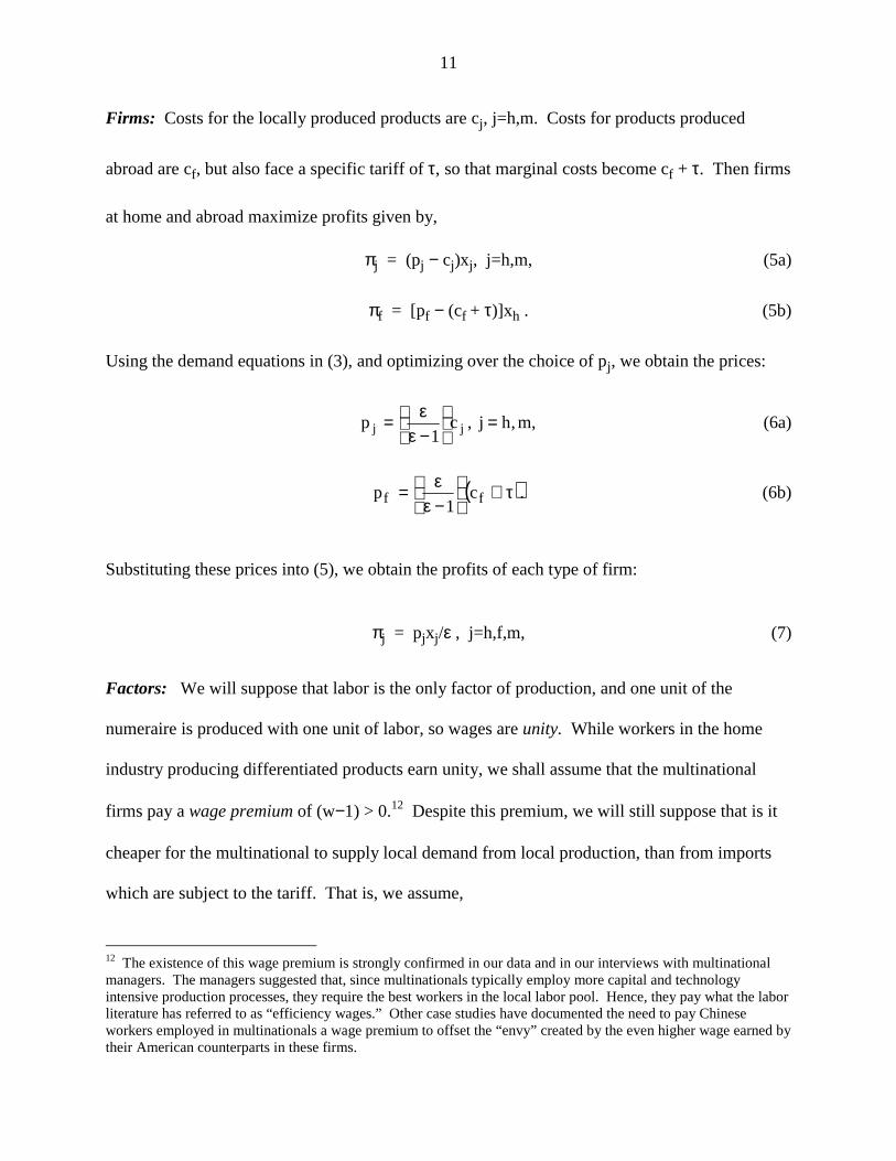
Firms: Costs for the locally produced products are cj, j=h,m. Costs for products produced

abroad are cf, but also face a specific tariff of τ, so that marginal costs become cf + τ. Then firms

at home and abroad maximize profits given by,

πj = (pj − cj)xj, j=h,m, (5a)

πf = [pf − (cf + τ)]xh . (5b)

Using the demand equations in (3), and optimizing over the choice of pj, we obtain the prices:

,m,hj,c1

p jj =

−εε= (6a)

( ).c1

p ff τ+

−εε= (6b)

Substituting these prices into (5), we obtain the profits of each type of firm:

πj = pjxj/ε , j=h,f,m, (7)

Factors: We will suppose that labor is the only factor of production, and one unit of the

numeraire is produced with one unit of labor, so wages are unity. While workers in the home

industry producing differentiated products earn unity, we shall assume that the multinational

firms pay a wage premium of (w−1) > 0.12 Despite this premium, we will still suppose that is it

cheaper for the multinational to supply local demand from local production, than from imports

which are subject to the tariff. That is, we assume,

12 The existence of this wage premium is strongly confirmed in our data and in our interviews with multinationalmanagers. The managers suggested that, since multinationals typically employ more capital and technologyintensive production processes, they require the best workers in the local labor pool. Hence, they pay what the laborliterature has referred to as “efficiency wages.” Other case studies have documented the need to pay Chineseworkers employed in multinationals a wage premium to offset the “envy” created by the even higher wage earned bytheir American counterparts in these firms.

12

cm < cf + τ . (8)

This assumption is needed to ensure that the multinational firms have any interest in entering the

local market.

Policy towards multinationals: Each foreign firm faces the decision of whether to supply

locally through imports, or through setting up a local plant which requires a fixed cost of F>0.

We suppose that the government also charges the multinational an profit tax of λ > 0. This

instrument is supposed to reflect the vast range of actual policies used in China to extract rents

from multinationals, and not just the nominal tax on multinationals. For example, the fact that

most multinationals have had to use local partners reflects an implicit tax on their profits, which

are shared with the partner; similarly, the land-use fees that are commonly charged reduce the

multinationals’ profits. By modeling these policies as a tax on profits, we are abstracting from

the inefficiencies caused by actual policies (such as local content restrictions, for example).13

This is similar to the “entry fee” used by Li and Chen (1998) , and is in the spirit of Grossman

and Helpman (1994), who draw on Bernheim and Whinston (1984) to argue that the outcome of

political contests can be efficient.

The profits earned locally are thus (1-λ)πm-F, with πm defined by (5a) and (6a).

Alternately, the multinational could just export to the home country, and earn πf defined by (5b)

and (6b). Thus, entry will occur if and only (1-λ)πm-F > πf. Using (7), this condition is written:

ε≥−

ελ− ffmm xp

Fxp

)1( . (9)

13 Of course, bribes paid to allow multinationals to enter are another example of the profit tax. Wei (1998) arguesthat corruption in China, which includes the need for “questionable payments”, acts as a significant deterrent toforeign direct investment.

13

We will assume that when m=λ=0 then (9) holds as a strict inequality. This means that for some

positive λ, entry of multinationals will occur.

Government Objective Function: We can now state the total returns to each interest group,

beginning with consumers/workers, who receive a weight of α in the objective function. It is

readily verified that maximized utility from (1) is U = I + q1-θ/(θ−1), where I denotes labor

income. With am workers used per unit output in the multinationals, the total wage premium is

(w−1)mamxm. The multinational’s price is pm=wamε/(ε-1), so the total wage premium can be

written [(ε-1)(w−1)/wε]mpmxm. Including this within labor income, we obtain utility of,

θ−

−θ+

−

−ε+= 1

mm q)1(

1xmp

w

1w

e

1LU

(10)

]xmpxp)mn(xpn[)1(

1xmp

w

1w1L mmfffhhhmm +−+

−θ+

−

ε−ε+=

where L is the labor endowment of the region. To obtain the second line of (10), we combine (3)

and (4) to solve for ]xmpxp)mn(xpn[ mmfffhhh +−+ = θ−1q .

We will suppose that the domestic firms are state-owned, so these profits accrue to the

regional and national government. Profits of the domestic firms are nhπh = nhphxh/ε, from (6).

We give revenue from state-owned firms a weight β in the objective function. Finally, the

government extracts rents mλπmfrom the multinationals, and also collects tariff revenue of

τ(nf − m)xf . These two sources of revenue are each given weights of unity.

The objective function for each region is defined as,

14

G(m,T,τ) ≡ αU + βnhπh + mλπm + τ(nf − m)xf

ffff

hhh xp)mn(p)1(

xpn)1(

L −

τ+−θα+

εβ+

−θα+α= (11)

mmxmpw

)1w)(1(

)1(

ελ+

ε−−εα+

−θα+ ,

where the equality follows using (10). Several properties of this function are summarized by:

Lemma 1

εθ−εβ−α

−ε−

=∂∂ )(

s)1(

)xpxp(

m

Gh

ffmm

−

−εθ−ε+

τ− )xpxp(1

sxpp ffmmfff

f(12)

−

−εθ−ε−

ελ+

−

ε−εα+ )xpxp(

1sxp

w

1w1ffmmmmm

where sj, j=h,f,m denotes the share of domestic spending on home, imported or multinational

products. Then:

(a) if

τ

εβ≥

ελ+

−

ε−εα

fp,max

w

1w1, then G is quasi-concave. If θ>1 these conditions

ensure that G is increasing, while if θ<1 then slightly stronger conditions are needed;14

(b) if

τ

εβ≤

ελ+

−

ε−εα

fp,min

w

1w1, then G is quasi-convex.

14 When θ<1 we need to multiply the right-hand side of the inequality in (a) by (ε-θ)/(ε-1)>1. Then for smsufficiently small, G will be increasing.

15

In (12), we show that ∂G/∂m consists of three terms. The first involves sh, the share of

home firms in domestic spending, and reflects the product market competition between the

multinationals and the home firms: if βsh is high as compared to α, then this term is negative.

The second term reflects the loss in import revenue as multinationals enter, as first analyzed by

Brecher and Diaz-Alejandro (1977). The third term reflects the wage premium generated by

employment in the multinationals and the profit tax levied on these firms, both of which generate

a gain in welfare.

Part (a) identifies conditions under which G is an increasing and quasi-concave function

of m, as illustrated in Figure 2 on the curve labeled “High wage premium or taxes.” It is well

known from Brecher and Diaz-Alejandro (1977) that when foreign capital is taxed at a

sufficiently high rate, this can reverse the decline in welfare that otherwise occurs from their

entry. Our model adds the gain due to the wage premium paid by multinationals. Conversely, if

the wage premium and taxes are low as in part (b), then G is instead a quasi-convex function of

m, as indicated by the curve labeled “Low wage premium and taxes.” In this case, it is relatively

easy to choose the value of β or of the tariff τ such that 0m/G =∂∂ in (12). Such a critical point

will be a global minimum of G, as illustrated.15

While Proposition 1 gives us the properties of G with respect to m, we do not suppose

that the government directly controls entry of multinationals. Instead, entry is influenced

through the tax rate λ and the tariff rate τ, so the number of multinational firms is written as a

function m(λ,τ). Multinationals react in the expected manner to changes in these policies:

15 A convex curve between home welfare and the inflow of foreign capital was illustrated by Brecher and Diaz-Alejandro (1977, Figure 2), when foreign capital was not being taxes. In their model, there was no wage premium.

16

Lemma 2

When (9) holds as an equality, then λd

dm < 0 and

τd

dm > 0.

We are now in a position to setup and solve the governments’ problem. We suppose that

the central and the regional governments jointly determine the rents appropriated from the

multinationals in each region. The central government also chooses the tariff rate. Denoting

regions by the subscript i, we let Gi[mi(λi,τ),λi,τ] denote the objective function for each region.

Then the profit tax and tariff are chosen to solve:

( )[ ]∑ τλτλτλ i

iiiii

,,,mG,

max , (13)

subject to mi(λi,τ) < nf, which is the maximum number of foreign firms willing to enter any

region. Our strong assumption in writing the objective function as in (13) is that the tax rate λi

for one region is separable from that in another region. This is an extreme version of Young’s

(1997) thesis that the provinces in China have only limited trade with each other. If there is no

trade between provinces, then they will not be in competition with one another for foreign

investment, because multinationals can only serve the market where they locate. While this case

does not literally apply in China, it is certainly true that foreign firm face restrictions on their

ability to market outside their immediate area.16 By assuming an extreme form of these

restrictions, we greatly simplify the governmental decision problem.

16 Some “native” Chinese firms face these restrictions as well. In interviews, one Chinese executive ruefully notedthat while the government has been bringing in “multinational” enterprises for twenty years, few truly“multiprovincial” enterprises are allowed to operate within China itself!

17

We also denote all other variables in region i with that subscript, though for simplicity we

suppose this does not apply to the foreign price pf , or the number of foreign firms nf. The

following result describes the solution to (13) over the choice of the tax rate λi, while a

discussion of the solution for tariffs τ is postponed until section 7.

Proposition 1

Suppose that Gi is increasing in mi. Then region i will choose the tax rate λi to allow entry of

multinationals to the point where either mi=nf or,

−

−λ−−

−εθ−ε

ε=

λ∂∂π−=

∂∂

fiif

imiiffmimi

i

imii

i

i smn

ms)1()xpxp(

1

1mm

m

G. (14)

A point satisfying (14) is a global maximum of Gi over the choice of λi provided that

τ

εβ≥

ελ+

−

ε−εα

fi

i

p,max

w

1w1, and also that smi < (ε-1)/(ε-θ) when (14) holds.

The optimality condition (14) is illustrated at point A in Figure 2, where the slope of the

curve Gi equals –miπmi /(∂mi/∂λi). This magnitude reflects the fall in the revenue λimiπmi when

the tax rate is lowered to attract more multinationals. That is, the regions are acting as

monopsonists as they attract foreign capital. This can be contrasted with the competition for

foreign capital that is often modeled between industrial countries or regions, and that is ruled out

in our framework by the assumption of limited trade between the regions.

18

Condition (14) leads to a global optimum under the conditions of Lemma1(a), and also

smi < (ε-1)/(ε- θ), which is automatically satisfied when θ>1 so that (ε-1)/(ε-θ)>1. If instead the

conditions of Lemma1(b) hold, so that Gi is quasi-convex in mi, then it is still possible for the

problem (13) to have an interior maximum: the fact that the regions are acting as monopsonists,

and recognize that multinational entry is affected by the profit tax, leads to further concavity in

Gi[mi(λi,τ),λi,τ] as a function of λi. In our estimation, we will confirm that the second-order

conditions are in fact satisfied.

We can now use the results from Proposition 1 to develop an estimating equation. We

add the subscript i to the variables in (12), and replace smi with 1-shi-sfi on the right-hand side.

This is set equal to the right-hand side of (14), as required for optimality. The resulting equation

can be simplified by using (9) as an equality. Finally, we also add a time subscript to all relevant

variables. We obtain the following equation for the share of spending on products of

multinationals in region i and year t:

fititf

itfit

ft

tfithit

it

it

it

ithitmit s

mn

ms

p)ss(

w

1w)1(

w

1wss

−

+

τε−+

−−εα+

−η+β−=

πλ+π

τε−

−θ−ε

−εα+πλ+θ−ε

πλ−ε+

θ−εαε+

)F(pw

1w

)(

)1(

)F)((

)1(

)( mititit

ft

ft

t

it

it2

mititit

mitit (15)

The first term on the right-side of (15) is the share of spending on domestic state-owned firms,

which enters with the coefficient -β. Thus, the weight on state-owned firms in the regional

objective function is simply obtained as the coefficient on their share in the regression (15). A

19

high weight on the state-owned firms indicates that in regions where these firms are more

prevalent, the share of multinational firms will be correspondingly reduced.

The next term on the right of (15) is the wage premium paid by multinationals, which has

the coefficient η≡α(ε-1)(θ-1)/(ε-θ). Following this is the wage premium times the share of

spending on state-owned firms plus imports. When the wage premium is higher, we expect that

regions would be more willing to accept multinationals, and this is confirmed by having a

positive coefficient α(ε-1) on that variable. The estimate of ε itself comes from the next term,

which is the ad valorem tariff rate times the share of spending on imports. This term reflects the

loss in tariff revenue as multinationals enter, and the coefficient is -ε. Thus, combined with the

former coefficient we can recover an estimate of α. The final term on the first line of (15)

reflects the number of multinationals times the share of imports. For simplicity we treat nf,

which is the number of foreign firms wanting to export or invest in China, as constant over

regions and time, and estimate it as a coefficient.

The terms on the second line of (15) are rather complex expressions of the profit tax

collected in each region, and the fixed costs of entry, entering themselves and interacted with the

wage premium and tariffs. We have no way of measuring these terms, but it seems very likely

that they will vary systematically across regions, and possibly also over time. Thus, we will

model the terms on the second line of (15) as:

,u)F(pw

1w

)(

)1(

)F)((

)1(itti

mititit

ft

ft

t

it

it2

mititit

mitit +δ+γ=

πλ+π

τε−

−θ−ε

−εα+πλ+θ−ε

πλ−ε(16)

where γi and δt and province and year fixed-effects, and uit is a random error assumed to be

uncorrelated with the variables on the first line of (15). Gathering all these terms into fixed-

20

effects plus an error is a strong assumption, but we have no other way of dealing with them.

With this assumption, we will be able to estimate (15) with two-stage least squares applied to

panel data.

Before turning to a discussion of the data, we remind the reader that we have assumed

that a multinational’s entry into one region will not affect its willingness to enter another region.

We could weaken this assumption somewhat by instead writing the constraint as Σi mi(λi,τ) < nf.

In that way, regions are competing for a fixed stock of foreign multinationals. If this constraint

is binding, it means that we would need to add a Lagrange multiplier onto the right of (14). This

multiplier would be time-dependent, and would also appear on the right of (15). But since it

would appear as a yearly fixed effect in (16), then the estimating equation is not affected.

A more significant change would be to consider instances where multinational entry is

not allowed, perhaps because Gi is declining in mi.17 These observations can be incorporated

into (15) by allowing the dependent variable to be zero, in which case the value of the right-hand

side should be negative. In other words, zero multinational presence can in principle be

incorporated into our estimation if we allow for a Tobit estimation. This raises technical

difficulties, however, because we also have fixed-effects as in (16), and some of the right-hand

side variables are endogenous (as discussed below). To date, there is no available estimator for a

censored model with fixed effects and endogenous variables. For this reason, we restrict the

dependent variable in (15) to positive values.18

17 If the weight on state-owned firms β is sufficiently large, for example, then Gi can be declining in mi even whenmultinationals are taxed at a high rate.18 A further difficulty with incorporating zero values for the dependent variable (i.e. when multinationals are notpresent in a province), is that some of the right-hand side variables are then not available. In particular, the wage-premium paid by multinationals, which appears on the right of (15) directly and as an interaction term, cannot bemeasured when there is no such activity in the province.

21

5. Data and Estimation Issues

We have three sources of data, described in increasing order of reliability. The first is a

collection of data from the provincial yearbooks for 1978-1995 (Xinjiang Statistical Bureau ,

1998). There are 30 provinces or autonomous regions distinguished in this source, and we will

refer to it henceforth as the “regional data.” This provides data on FDI, employment, wages, and

output, with the latter broken down by state-owned firms, multinationals, collectives, and

individual proprietorships.19 The wage data does not begin until 1984, effectively limiting our

sample to 1984-1995. It distinguishes the wages paid per worker in multinationals, state-owned

enterprises, and urban collectives, with that in multinationals usually being the highest and that

in urban collectives usually the lowest.20 The wage premium was constructed in two ways. The

first method (called unweighted) was to compute it as the wages paid by multinationals minus

that in urban collectives, divided by that in multinationals. The second, possibly more accurate

method (called weighted), was to compute the wage premium as the wages paid by

multinationals minus a weighted sum of the wages paid in state-owned enterprises and urban

collectives, using employment shares (from the regional data) as weights, with this difference

divided by the multinational wage.

The second data source was various editions of the Chinese Statistical Yearbooks, which

we judge to be more reliable than the provincial yearbooks. In the case of discrepancies, the

provincial output data for state-owned firms, multinationals, collectives, and individual

19 In early years, there is no category exclusively for multinational (or foreign invested enterprises). Rather, thereis a category of output attributed to “other” firms, which includes both multinationals and other stock-heldcompanies. In later years, it was possible to separate out the stock-held companies from the multinationals usingdata provided. In early years this was not possible, except that we did restrict the output share of multinationals tobe zero until another series for “foreign capital actually invested” became positive.20 As in the previous footnote, in early years there is no category exclusively for multinational wages, but there is“other” wages that includes both multinationals and other stock-held companies. In later years, we could comparethis “other” category with actual wages paid by multinationals, and found that they followed each other very closely.The correlation coefficient between the two series was 0.905.

22

proprietorships have been replaced with the corresponding figures from the Statistical

Yearbooks, when the latter had this data. In a limited number of cases for 1984-1985, provincial

output data for state-owned firms, multinationals, collectives, or individual proprietorships had to

be imputed based on employment in these categories.

The third data source was the Chinese trade data obtained from the Customs General

Administration as part of the project described in Feenstra, Hai, Woo and Yao (1998, 1999).21

This source gives imports and exports broken down by Chinese province, the kind of Chinese

enterprise involved in the trade (state-owned enterprise, foreign-invested enterprise, other), and

the type of trade regime under which the transaction took place (ordinary trade, processing trade,

other), for 1988-1995. We judge this to be our most reliable data source, and use it to correct the

trade data from the provincial yearbooks, as described below.

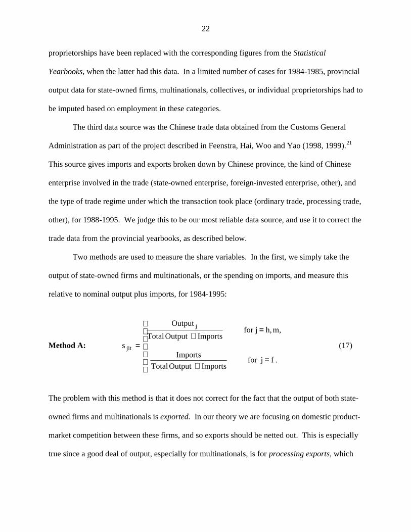
Two methods are used to measure the share variables. In the first, we simply take the

output of state-owned firms and multinationals, or the spending on imports, and measure this

relative to nominal output plus imports, for 1984-1995:

Method A:

=+

=+

=

.fjforImportsOutputTotal

Imports

m,h,jforImportsOutputTotal

Output

s

j

jit (17)

The problem with this method is that it does not correct for the fact that the output of both state-

owned firms and multinationals is exported. In our theory we are focusing on domestic product-

market competition between these firms, and so exports should be netted out. This is especially

true since a good deal of output, especially for multinationals, is for processing exports, which

23

means that intermediate inputs are imported, had some value-added, and then exported again.

The use of nominal output will greatly overstate the actual value-added in these activities. By

the same token, the use of nominal imports in the Method A will greatly overstate the imports

that are not intended for processing, and potentially compete with state-owned firms.

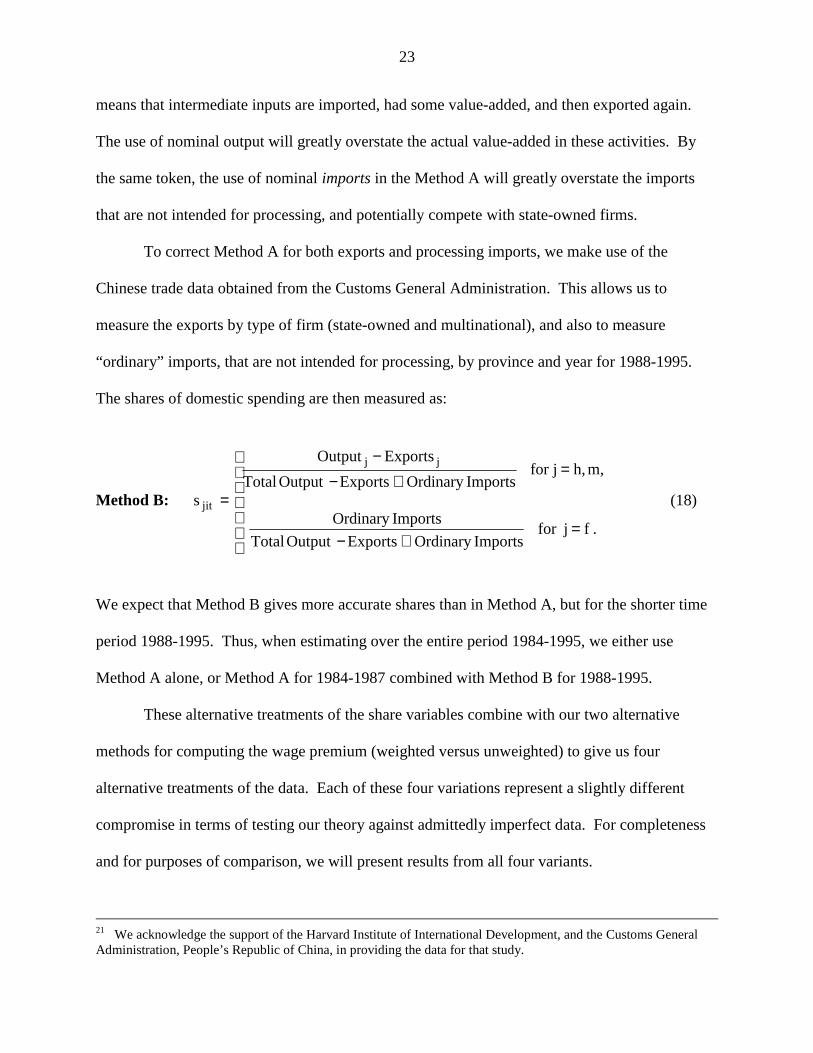
To correct Method A for both exports and processing imports, we make use of the

Chinese trade data obtained from the Customs General Administration. This allows us to

measure the exports by type of firm (state-owned and multinational), and also to measure

“ordinary” imports, that are not intended for processing, by province and year for 1988-1995.

The shares of domestic spending are then measured as:

Method B:

=+−

=+−

−

=

.fjforImportsOrdinaryExportsOutputTotal

ImportsOrdinary

m,h,jforImportsOrdinaryExportsOutputTotal

ExportsOutput

s

jj

jit (18)

We expect that Method B gives more accurate shares than in Method A, but for the shorter time

period 1988-1995. Thus, when estimating over the entire period 1984-1995, we either use

Method A alone, or Method A for 1984-1987 combined with Method B for 1988-1995.

These alternative treatments of the share variables combine with our two alternative

methods for computing the wage premium (weighted versus unweighted) to give us four

alternative treatments of the data. Each of these four variations represent a slightly different

compromise in terms of testing our theory against admittedly imperfect data. For completeness

and for purposes of comparison, we will present results from all four variants.

21 We acknowledge the support of the Harvard Institute of International Development, and the Customs GeneralAdministration, People’s Republic of China, in providing the data for that study.

24

Estimation of (15) requires that we correct for endogeneity of the regressors. This occurs

because the dependent variable and some independent variables are shares of domestic spending,

and in our theory sum to unity: smit+shit+sfit=1. Thus, the share of spending on multinational

output smit (which appears on the left of 15), and the share of spending on state-owned firms shit

(which appears on the right), would tend to have a correlation of –1 by construction. We correct

for this in several ways. When we measure the share of spending on multinationals, state-owned

firms, and imports, we include the spending on products from collectives and individual

proprietorships.22 This means that the shares smi, shi, and sfit sum to less than unity.

Furthermore, we include the spending on collectives and individual proprietorships as control

variables on the right of (15). For example, a reduction in spending on products from collectives

will increase all of smit, shit, and sfit , which would tend to create a positive correlation between

smit and shit in (15); including the spending on collectives and individual proprietorships as

controls offsets this bias. Finally, we use instrumental variables when estimating (15).23

A selection of the data for 1995 is shown in Table 1. For convenience, we report the data

according to three regional groupings: Beijing and the neighboring industrial province of Tianjin;

all those provinces that are coastal, and contain at least one “open coastal city” or SEZ; and then

the interior provinces. For the coastal provinces, the ordering runs north to south; while for the

interior provinces, the order runs roughly clockwise from north to south, and then circling around

to the far inland provinces. It is readily apparent that some coastal provinces have a share of

domestic spending on products of multinationals that equals or exceeds that for state-owned

22 That is, Total Output appearing in the denominator of (17) and (18) includes the output of collectives andindividual proprietorships, as does Exports in (18).23 The instruments are the nominal sales of state-owned firms, value of imports, lagged FDI stock, output, wagepremium, the interaction between the wage premium and these four variables, as well as the two control variables.

25

enterprises; the average of these two shares is 14.4% and 20.2% respectively.24 In contrast, the

interior provinces have an average share of multinationals and state-owned enterprises of 3.5%

and 55.1%, respectively. This illustrates the much more limited multinational presence in the

interior provinces, where the state plays a greater role.

Of course, this difference in the relative presence of multinationals versus state-owned

firms in the coastal and interior provinces can be explained by the natural tendency of the

multinationals to locate where transportation is easier, combined with the deliberate decision of

Chinese planners to develop state-owned enterprises in the inland regions. In our estimation, we

fully control for these differences by including fixed effects across provinces (and also fixed

effects for each year). Thus, the identification of the political weights on stated-owned

enterprises versus consumers will come from the time-series variation within each province, over

1984-1995, and not from the cross-sectional variation that is so apparent in Table 1.

Two other variables are also needed to estimate (15). As a proxy for the number of

multinational firms mit in a province in a given year, we use the cumulated stock of foreign

direct investment actually utilized (in billions of US$). This was computed by taking flows of

foreign direct investment from the regional data and cumulating them using a depreciation rate of

4.5%.25 The 1995 value for this variable was shown in Figure 1. It is interacted with the import

share sfit on the right of (15), and the coefficient is then 1/(nf-mit). For simplicity, we suppose

24 Note that for Guangdong, the “zero” share for state-owned enterprises in 1995 arises because the exports of theseenterprises from the Chinese customs data exceeds their output from the provincial yearbooks or Chinese StatisticalYearbooks. This reflects a discrepancy between the two data sources, but we can still presume that the output ofstate-owned enterprises in Guangdong for domestic consumption is small.25 This depreciation rate was based on data drawn from the 1994 Benchmark Survey on U.S. direct investmentabroad conducted by the Bureau of Economic Analysis of the U.S. Department of Commerce. We are grateful toMichael Ferrantino of the International Trade Commission for drawing our attention to this document, andperforming the computation that produced this number. However, we note that our results are not sensitive to theassumed rate of depreciation, and we obtain similar results with a depreciation rate of zero.

26

that nf is large enough so that this coefficient can be treated as constant over time and regions,

and re-write it as 1/nf when estimating (15).

Finally, the tariff variable is computed for province i in year t as a weighted average of ad

valorem tariffs, based on the provincial imports of different goods multiplied by the 1996 tariff

rate assessed on those good. Unfortunately, we did not have access to any earlier years of tariff

data. However, we were able to include in this calculation an indicator variable, equal to one

when that product is also exported by FIEs in the province, and zero otherwise. Thus, the

weights used to compute the average tariff were the provincial imports of different goods times

the indicator variable, indicating whether the good was also exported (and therefore produced)

by FIEs. This was done because the tariffs we are really interested are those on imported goods

that potentially compete with local FIE-produced goods. Including this indicator variable ensures

that only those imports which potentially compete with local FIE-produced goods are included in

the weighted average tariff level.26 These average provincial tariff levels are shown in the last

column of Table 1. Because this variable was constructed using the tariff schedule in only one

year (1996), it actually varies across provinces i rather than years t. Thus, it is re-written as τi

rather than τt in (15).

6. Estimation Results

Results from regressions based on (15)-(16), using data for 1984-1995, are presented in

Table 2. Each of the four columns uses a different variant of the wage premium and the share

data. The overall results are broadly similar in all variants, although the exact parameter

26 We do not have disaggregated data on FIE production, but we do have disaggregated data on FIE exports. Ourpresumption is that if FIEs are exporting a good from a Chinese province, then they are also probably selling somequantity of that good on the local market, or that at least the potential for local sales exists.

27

estimates do vary. We also note that our key parameters are estimated with varying degrees of

precision in these four columns. Standard errors are placed in parentheses below the respective

parameter estimates.

Each regression includes a full set of provincial and year fixed effects. An estimate of

the parameter β, the weight of state-owned enterprise output in the government’s objective

function, can be taken from the regression coefficient on the state-owned share. This coefficient

is always statistically significant and, usually larger (in absolute value) than unity, though not

significantly so. Estimates of α, the weight on consumer welfare, can be derived from the

regression coefficients shown in the third and fourth rows of Table 2. These estimates are

reported in the first row of Table 3, where we also repeat the estimates of β and ε. Despite some

difference in the estimates over our four variations, a striking pattern emerges: we find that the

weight applied to consumer welfare is much lower than that applied to the output of state-owned

enterprises, with their ratio between one-fifth and one-twelfth in our estimates.

Turning to the other coefficients in Table 2, an estimate of θ can be derived from the

coefficient on the wage premium. The point estimate for θ is always negative, which contradicts

our assumption in (1), but a 95% confidence interval constructed from the other coefficients

includes both positive and negative values. Thus, our estimation fails to identify this parameter

with any precision. The coefficient 1/nf takes the value 0.014-0.023 in Method A, and inverting

this, we estimate that there is $40-70 billion of foreign capital ready to invest in any region of

China. This parameter is estimated with the wrong sign in Method B, however.

We can make use of our parameter estimates to check that the second-order conditions

for the maximization problem (13) are satisfied. Proposition 1 provides us with sufficient

conditions that are easily checked, depending on the choice of λi. However, given the tariffs

28

reported in the last column of Table 1, and the parameter estimates in Table 3, these sufficient

conditions are not satisfied even for very high choices of the profit tax λi. Instead, we need to

directly compute the second-derivative of Gi[mi(λi,τ),λi,τ] with respect to λi, as done in the

Appendix. This second-derivative is evaluated at the critical point (14). For the choice of

parameters ε=5, θ=0.5, β=1, α=0.2 and1/nf = 0.02, we find that the second order condition is

satisfied for every province provided that λi >0.18. Using higher values of the elasticities ε=10

and θ=2, the second-order conditions are satisfied provided that λi >0.26. These values are well

within the range of actual tax rates in China (15% in the SEZ and 24% in the open coastal cities),

without even including the many other ways that rents are extracted from multinationals. We

conclude, therefore, that our objective function is “well behaved.”

The use of instrumental variables raises the question of the validity of the instruments.

To assess this, we regress the residuals from the estimated equations on the instruments, and

report in Table 2 the χ2 statistic constructed as NR2 from this regression. We note that this

approach has been criticized in the econometrics literature for a tendency to “over-reject” the

null hypothesis of validity of the over-identifying restrictions. Indeed, in one of our four

regressions, the null hypothesis of validity is rejected at the 5% level, as the χ2 test statistic is

(slightly) larger than the critical value of 9.49. Otherwise, the null hypothesis is easily accepted

at conventional levels.

A breakdown of the implied structural coefficients of interest is provided in Table 3 for

later sub-samples of the data, the 1988-1995 period and the 1990-1995 period. As we confine

our view to the later sub-samples, we lose observations and consequently precision in some of

our estimates; sub-periods smaller than 1990-1995 do not yield many significant coefficients at

29

all. In the later sub-periods, the estimated magnitudes of the weight on state-owned enterprises

falls. Likewise the weight on consumer welfare rises. This is consistent with the historical trend

towards liberalization, of course. However, the gap between the two weights remains

substantial: for the relatively liberal 1990-95 sub-period, we find that the weight on consumer

welfare is still only about one-half of the weight on state-owned enterprises. This is consistent

with the pessimism among some China scholars concerning the momentum of reform of

restrictions on FDI and trade.

7. Choosing the Tariffs

At the beginning of the paper, we motivated our topic by the desire of China to enter into

the WTO, and suggested that the existing trade barriers would have to be reduced substantially to

achieve this goal. To what extent does the presence of multinationals interact with that goal?

The willingness of foreign firms to invest in China certainly reflects, in part, the difficulty of

importing there directly. If tariffs are reduced substantially, this raises the distinct possibility

that foreign firms who are not just involved in processing trade will divest of some of their

holdings. This scenario was explicitly mentioned in some of our field interviews, and reflects

the fact that for firms not involved in processing trade, investment in China is an attempt to

access the huge domestic market; low wages play only a secondary role.

If we accept this characterization of foreign direct investment, it suggests that a reduction

in tariffs may lead to an outflow of foreign direct investment. There is no “natural experiment”

that allows us to directly estimate this from data for China. However, we can use the estimates

from the previous section to construct the outflow that is consistent with our theoretical model, in

an attempt to judge the welfare impact.

30

To compute the welfare effects, we begin by characterizing the optimal tariff in a special

case. Suppose that the government does not care about state-owned profits (β=0), there are no

multinationals (mi=0), and the tariff is applied to a single import variety . Then it can be shown

that in this simple case, the optimal tariff which maximizes (13) is:

−εα−

ε=τ

1

1

p

*

f . (19)

To interpret this condition, suppose that α=0 so the government did not care about consumer

welfare. Then τ*/pf =1/ε is the revenue maximizing tariff. As α > 0 then the optimal tariff is

reduced below this level.27

Now consider the total effects of a change in tariff on welfare, given that β, mi >0 and the

multinational profit tax *iλ has been chosen optimally. We compute the change in the objective

function of a single region Gi[mi(*iλ ,τ), *

iλ ,τ] as:

.d

dm

G

mmm

G

m

m

GG

d

dG

im

imii

i

i

iimii

i

i

i

iii

τλ

π+τ∂

∂=

λ∂∂

τ∂∂π−

τ∂∂=

τ∂∂

∂∂

+τ∂

∂=

τ

(20)

27 Note that if α=1 so that consumer welfare and revenue receive the same weights, then the optimal tariff isnegative. The reason for this is that with a specific tariff and constant percentage markup (due to CES preferences),then the “terms of trade effect” is negative: raising marginal costs using the tariff leads to an even greater increase inimport prices, implying that the net-of-tariff price goes up instead of down. It follows that an import subsidy isoptimal. For the range of α<1 in our estimates, however, we certainly obtain a positive value for the optimal tariff τ*in (19), due to its revenue impact.

31

The first line of (20) uses the envelope theorem, whereby we can hold *iλ constant when

computing the effect on Gi of changing τ. The second line makes use of the first-order condition

(14), and then the third line follows by computing 0ddimi >τλ as the slope of an iso-curve of

mi(λi,τ). Thus, the total impact of decreasing tariffs can be interpreted as: (i) the direct impact

holding the profit tax and number of multinationals fixed; and (ii) the indirect effect through

decreasing the profit tax itself so that multinationals do not exit the country.

Given this interpretation, we now compute each of the components (i) and (ii) from our

model. Because the tariff is specific, it useful to measure it relative to foreign prices pf, and we

also measure the regional objective function relative to total imports if the differentiated good,

denoted by Mi ≡ (nf-mi)pfixfi :

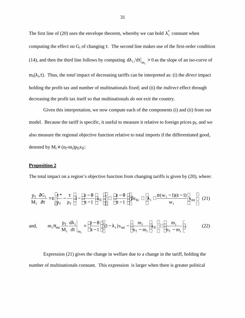
Proposition 2

The total impact on a region’s objective function from changing tariffs is given by (20), where:

−ε−α+λ+β

−ε

θ−ε+

−ε

θ−ε−τ−τε=τ∂

∂mi

i

iihifi

ff

i

i

f sw

)1)(1w(s

1s

11

pp

*G

M

p(21)

and,

−

+

−

−λ−

−εθ−ε=

τλ

πif

ifi

if

imii

m

i

i

fmii mn

ms

mn

ms)1(

1d

d

M

pm

i

. (22)

Expression (21) gives the change in welfare due to a change in the tariff, holding the

number of multinationals constant. This expression is larger when there is greater political

32

weight on state-owned enterprises, or wage premia paid by multinationals: these considerations

mean that increases in the tariff above the “simple” optimum in (19) will raise welfare, whereas

tariff reductions potentially lower welfare. Expression (22) takes into account the induced

effects of tariff changes on the profit tax obtained from multinationals. Since this expression is

positive, is leads to a welfare loss from any tariff reduction.

The unweighted average of the 1996 tariffs in China is 23.4%, and under its WTO

accession proposal the tariffs in 2005 would be reduced to 16.2%, or three-quarters of their 1996

value.28 Applying this reduction to the 1996 tariffs used in our estimation (the last column of

Table 1), we obtain the proposed WTO tariffs shown in the first column of Table 4, at the

provincial level. Then using this change of tariff from their 1996 level to the WTO proposal, we

evaluate the welfare impact from Proposition 2, with results shown in Table 4.

In the first example of Table 4, we use low values of the elasticities: ε=5 and θ=0.5. We

also use the weight on consumer welfare of α=0.2, a weight on state-owned firms of β=1, and a

value of 1/nf = 0.02, which are consistent with our earlier estimates. The “simple” optimal tariff

in (19) for these parameters is τ*/pf = 0.15. The direct effect of lowering the tariffs is computed

from (21), and the indirect effect through lowering the profit tax for multinationals is computed

from (22).29 We see that the direct welfare effect varies in sign over the provinces. Beijing has a

direct welfare benefit of 2% of its import value, reflecting its rather high initial tariff (41% in

Table 1), whereas Liaoning has a direct welfare loss because its initial tariff (23%) is less than

the provincial optimum, taking into account the weight given to state-owned firms and wage

28 These unweighted tariffs are reported in World Bank (1997, Annex Table A.1). If we take the longer periodfrom 1992 to 2005, then unweighted tariffs are reduced by one-half. Thus, to evaluate this total change, the welfareeffects in Table 4 should all be doubled.

33

premia. However, the indirect impact of lowering the profit tax for multinationals means that the

gains to Beijing from tariff reduction are more than offset, and the total impact of tariff reduction

becomes negative. This reversal of the direct gains, leading to overall losses, is also found for

the neighboring industrial region of Tainjin, and nearly so for Fujian. These regions illustrate the

idea that the losses through potential departure of multinationals can offset the direct gains from

tariff reduction, making such liberalization politically difficult to achieve. This is reinforced by

the negative direct effect of tariff reductions found for quite a number of other provinces.

In the second example we consider higher elasticities: ε=10 and θ=2. Higher values for

either of these elasticities make it more likely that welfare gains will be found from tariff

reduction. Other parameters are as before (α=0.2 and β=1), so the “simple” optimal tariff in (19)

is now τ*/pf = 0.078. We find that nearly all regions now have direct gains from tariff removal,

which are substantially larger than the indirect losses. For example, Beijing has a direct gain of

20.4% of its import value, which is much larger than the 2% indirect loss due to potential exit of

multinationals. Gains of a smaller magnitude are observed for most other provinces. Thus, with

high values for the elasticities, most provinces gain from the proposed reduction of tariffs under

China’s WTO proposals, but for low values of the elasticities this is not the case. Both these

cases are within the range of elasticities (for ε) that we have estimated. So while we are not able

to make more definite conclusions about the potential losses due to multinational exit, and

whether these offset the gains due to tariff removal, this possibility is certainly within the range

of our estimates.

29 Note that both (21) and (22) depend on λ, but that this term enters in an exactly offsetting way in eachexpression. Thus, the total effect does not depend on value specified for λ, so we exclude this term from thecalculation of (21) and (22) individually.

34

8. Conclusions

After two decades of substantial reform, China’s current trade and foreign investment

regime remains far from open. If ever we needed a theoretical framework to explain sharp

deviations of policy away from that proscribed by laissez faire economics, we need it here. Our

paper represents a first attempt to apply a theoretical model based on Grossman and Helpman

(1994, 1996) to a policy context in which “political economy” considerations are essential for

understanding and predicting the trajectory of economic reform, and then to obtain economically

meaningful estimates of the model’s parameters from Chinese economic data.

As in any ambitious attempt to marry a complicated structural model with imperfect data,

we have been driven to make a number of compromises. Nevertheless, the results that we end

with are quite striking. To summarize, using the estimates based on our full sample, we find that

the weight applied to consumer welfare is between one-fifth and one-twelfth of the weight

applied to the output of state-owned enterprises. We find that governmental preferences have

shifted over time, but even if we estimate the model with data from the relatively liberal 1990-95

sub-period we still find that the weight on consumer welfare is only about one-half of the weight

on state-owned enterprises. Finally, we estimate the impact on regional governmental objectives

of the proposed changes in tariff structure that China has put forth as part of its bid for WTO

accession. We find that these changes could potentially lower the regional objective function,

due to the exit of multinationals. While this result is sensitive to the elasticities that are used, it

provides some quantitative backing for skepticism that China, given the current political

equilibrium, would actually follow through with the proposed liberalization.

There are a number of directions in which we hope to move this research in future papers.

Most will involve more disaggregated data on multinational and state-owned production and

35

trade. It is obvious that government and other barriers differ in systematic ways across

industries, and part of the provincial variance that we are picking up in our data is really

attributable to differences across provinces in industry mix. Anecdotal evidence also suggests

that there are important differences in the nature of multinationals depending on the “source

country.” In particular, firms are affiliated with Taiwanese or Hong Kong-based foreign partners

are overwhelmingly concentrated on production for export, and hence are to a great extent

outside our modeling framework. With more disaggregated data, we could focus on the Western

and Japan-affiliated multinationals that tend to be more focused on the Chinese market, and

therefore more relevant for our model. To this end, we are currently building up an FDI data

base at the project level.

Further refinements in the model might also prove worthwhile. While a more realistic

depiction of the actual restrictions placed on multinationals (such as local content and export

requirements) would complicate the model, it would also likely yield much more accurate

estimates of the real relative weight placed on consumer welfare. If anything, our current

estimates may prove to be an upper bound of the weight actually placed on consumer welfare by

the Chinese government.

36

Appendix

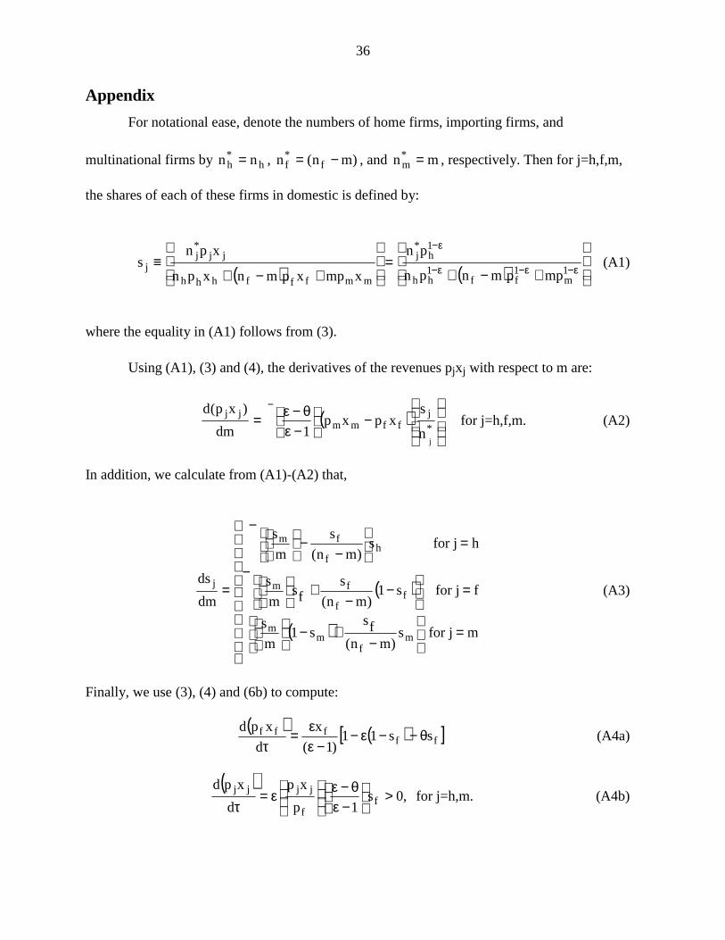
For notational ease, denote the numbers of home firms, importing firms, and

multinational firms by h*h nn = , )mn(n f

*f −= , and mn*

m = , respectively. Then for j=h,f,m,

the shares of each of these firms in domestic is defined by:

( ) ( )

+−+=

+−+≡ ε−ε−ε−

ε−

1m

1ff

1hh

1h

*j

mmfffhhh

jj*j

jmppmnpn

pn

xmpxpmnxpn

xpns (A1)

where the equality in (A1) follows from (3).

Using (A1), (3) and (4), the derivatives of the revenues pjxj with respect to m are:

( )

−

−εθ−ε=

−

*

jffmm

jj

jn

sxpxp

1dm

)xp(dfor j=h,f,m. (A2)

In addition, we calculate from (A1)-(A2) that,

( )

( )

=

−

+−

=

−

−+

−

=

−

−

−

=

mjfors)mn(

fss1

m

s

fjfors1)mn(

sfs

m

s

hjfors)mn(

s

m

s

dm

ds

mf

mm

ff

fm

hf

fm

j(A3)

Finally, we use (3), (4) and (6b) to compute:

( ) ( )[ ]fffff ss11

)1(

x

d

xpd θ−−ε−−ε

ε=τ

(A4a)

( ),0s

1p

xp

d

xpdf

f

jjjj >

−εθ−ε

ε=

τ for j=h,m. (A4b)

37

Proof of Lemma 1

Using (A2), we compute the derivative of G as:

( ) ( )( )

ε

λ+

ε−ε−

+τ

+ε

β+

−θα−

−εθ−ε=

∂∂ mm

f

fhffmm

s

w

s)1(1w

p

ss

1xpxp

1m

G

( ) ( )( )

ε

−ε−+−θ

α+

τ+−θ

−w

)1(1w

1

1xp

p1

1xp mm

fff , (A5)

which can be re-written as (12). Substituting sm=1-sh-sf, this can be re-arranged as:

( )

ελ+

ε−ε−α+

−θα−

−ε−θ+

τ−ελ+

ε−ε−α=

∂∂

w

)1)(1w(

)1(xpxp

1

1

pw

)1)(1w(xp

m

Gffmm

fff

τ−ελ+

ε−ε−α+

εβ−

ελ+

ε−ε−α−

−εθ−ε+

ffhffmm pw

)1)(1w(s

w

)1)(1w(s)xpxp(

1(A6)

Using (A1)-(A3), we compute from (A6) ,

( ) m

G

mn

s

m

s

1m

G

f

fm2

2

∂∂

−

−

−εθ−ε=

∂∂ −

(A7)

( ) ( )

( )( )

−

−+

ελ−

ε−ε−α−τ+

−

−

ελ−

ε−ε−α−

εβ−

−εθ−ε+

ff

ff

m

f

hf

fmffmm

s1mn

ss

m

s

w

)1)(1w(

p

smn

s

m

s

w

)1)(1w(xpxp

1

Eq. (8) ensures that pmxm- pfxf > 0. Then the hypothesis of part (a) implies that ∂2G/∂m2 < 0

when ∂G/∂m = 0, so that G is quasi-concave When θ>1 we also obtain ∂G/∂m > 0 from (A6),

38

while when θ<1 then slightly stronger conditions are needed. Under the hypothesis of part (b),

we see that ∂G/∂m = 0 in (A7) implies that ∂2G/∂m2 > 0, so that G is quasi-convex.

Proof of Lemma 2

Treating (9) as an equality, the derivatives with respect to m are given by (A2). Then totally

differentiating (9), we obtain,

( )[ ] .0)mn/(mss)1(xpxp

xmp1

d

dm

ffmffmm

mm <−−λ−−

θ−ε−ε−=

λ(A9)

Again treating (9) as an equality, we can totally differentiate and use (A2) and (A4) to obtain,

( )[ ] .0

)mn/(mss)1()xpxp(

xp)1(s]xpxp)1[(mp

d

dm

ffmffmm

fffffmmf >

−−λ−−−ε+−λ−θ−ε

θ−εε=

τ(A10)

Proof of Proposition 1

(a) The first-order condition for an interior maximum of (13) with respect to λi is:

0d

m

m

GG

d

dG

i

i

i

i

i

i

i

i =λ

∂∂∂

+λ∂

∂=

λ. (A11)

Noting that ∂Gi/∂λi = miπmi, and using (A9), this condition is expressed as (14).

To check the second-order condition, for fixed τ we solve for the profit tax λi=φi(mi,τ) as

a function of the number of multinational firms. Then we re-express the optimization problem

(13) as choosing mi subject to 0 < mi < nf to maximize Σi Gi[mi,φi(mi,τ),τ]. The first-derivative

39

is dGi/dmi = ∂Gi/∂mi + miπmi∂φi/∂mi = ∂Gi/∂mi + miπmi/(∂mi/∂λi). Using (A1)-(A3), (A7) and

(A9), it can be shown that:

2if

fiimii

i

i

i

i2i

i2

)mn(

sm

12

dm

dGby replaced

m

G with (A7)

dm

Gd

−

−εθ−επλ−

∂∂

=

( )

πλ+

−εθ−ε−πλ+−+π

−

−

λ−

−εθ−ελ+ )F2(s

1)F(sF2

mn

s

m

s)1(

1 miiitmimiiitmiitmiif

fi

i

miii

When dG/dm = 0, then d2G/d2m < 0 provided that the second line is non-negative. Using πmi =

λiπmi + Fit + πf, a sufficient condition for this is smi < (ε-1)/(ε-θ).

To evaluate this second-derivative numerically, we can divide by total expenditure on the

differentiated good, so that πmi=pmixmi /ε becomes substitute for smi/(mε). We also need to

specify the fixed costs Fit, and we choose the conservative value of zero, which leads to a higher

value for the second-derivative.

Proof of Proposition 2

Differentiating (11) using (A4), the partial derivative with respect to τ is,

( )iififi LGs

1p

Gα−

−εθ−ε=

τ∂∂ ( )

ετ−−θ

εα−−+f

fifif p)1(1xpmn . (A12)

Substituting for Gi from (11), and simplifying, we obtain (21). To obtain (22), we compute

)m()m(dd iiimii

λ∂∂τ∂∂−=τλ from (A9) and (A10), and simplify.

40

References

Bernheim, Douglas B. and Michael D. Whinston, 1986, “Menu Auctions, Resource Allocation,and Economic Influence,” Quarterly Journal of Economics, 101, 1-31.

Brecher, Richard and Carlos Diaz-Alejandro, 1977, “Tariffs, Foreign Capital and ImmiserizingGrowth,” Journal of International Economics, 7, 317-322.

Feenstra, Robert C., Wen Hai, Wing T. Woo, and Shunli Yao, 1998 “The U.S.-China BilateralTrade Balance: Its Size and Determinants,”, NBER Working Paper no. 6598.

Feenstra, Robert C., Wen Hai, Wing T. Woo, and Shunli Yao, 1999, “Discrepancies inInternational Data: An Application to China-Hong Kong Entrepôt Trade,” AmericanEconomic Review, May, forthcoming.

Grossman, Gene M and Elhanan Helpman, 1994, “Protection for Sale,” American EconomicReview, 84, 833-850.

Grossman, Gene M and Elhanan Helpman, 1996, “Foreign Investment with EndogenousProtection,” in Robert C. Feenstra, Gene M. Grossman and Douglas A. Irwin, eds., ThePolitical Economy of Trade Policy: Papers in Honor of Jagdish Bhagwati, Cambridge:MIT Press, 199-224.

Grub, Phillip Donald and Jian Hai Lin, 1991, Foreign Direct Investment in China, New York:Quorum Books.

Lardy, Nicholas, 1992, Foreign Trade and Economic Reform in China, 1978-1990. New York:Cambridge University Press.

Li, David D. and Qi Chen, 1998, “Why Aren’t Foreign Direct Investments Always Welcome? –A Political Economy Analysis,” University of Michigan, mimeo.

Naughton, Barry, 1995, Growing Out of the Plan: Chinese Economic Reform, 1978-1993. NewYork: Cambridge University Press.

Naughton, Barry, 1996, “China’s Emergence and Prospects as a Trading Nation,” BrookingsPapers on Economic Activity, 2: 1996, pp. 273-343.

Pomfret, Richard W. T., 1991, Investing in China: Ten Years of the Open Door Policy. Ames:Iowa State University Press.

Rosen, Daniel, 1998, Behind the Open Door: Foreign Firms in China, Institute for InternationalEconomics, Washington, D.C.

Sachs, Jeffrey D. and Wing Thye Woo, 1997, “Understanding China’s Economic Performance,”NBER Working Paper no. 5935, February.

41

Steinfeld, Edward, 1998, Forging Reform in China: The Fate of State-Owned Industry, NewYork: Cambridge University Press.

Wei, Shang-Jin, 1998, “Why Does China Attract so Little Foreign Investment?” HarvardUniversity and NBER, mimeo.

World Bank, 1997, China Engaged: Integration with the Global Economy. Washington, D.C.

Xinjiang Statistical Bureau , 1998, “China’s Regional Economy in the 17 Years Since Reformand Liberalization” electronic database on diskette.

Young, Alwyn, 1997, “The Razor’s Edge: Distortions and Incremental Reform in the People’sRepublic of China, University of Chicago, mimeo.

42

Table 1: Selected Data in 1995

Output MultinationalShare

State-ownedShare

ImportShare

WagePremium

Tariffs

Beijing 1909 0.215 0.555 0.075 0.366 0.413Tianjin 2094 0.240 0.284 0.043 0.522 0.306

Include “Open Coastal Cities” or SEZLiaoning 4975 0.042 0.389 0.022 0.475 0.227Hebei 3996 0.066 0.327 0.007 0.360 0.289Shandong 8456 0.054 0.274 0.007 0.308 0.282Jiangsu 11813 0.102 0.176 0.008 0.353 0.223Shanghai 5129 0.290 0.294 0.080 0.452 0.163Zhejiang 8088 0.075 0.082 0.010 0.270 0.240Fujian 2801 0.270 0.068 0.035 0.387 0.298Guangdong 9535 0.271 0.000 0.075 0.330 0.215Guangxi 1666 0.065 0.357 0.014 0.357 0.252Hainan 193 0.204 0.054 0.348 0.436 0.172

Average 5665 0.144 0.202 0.061 0.373 0.236Do not include “Open Coastal Cities” or SEZ

Heilongjiang 2204 0.026 0.648 0.011 0.582 0.264Jilin 1429 0.062 0.576 0.054 0.367 0.174Inner Mongolia 782 0.048 0.606 0.021 0.232 0.320Shanxi 1754 0.017 0.433 0.005 0.399 0.216Henan 4715 0.041 0.323 0.006 0.352 0.294Anhui 3156 0.032 0.292 0.005 0.578 0.241Hubei 4103 0.037 0.354 0.013 0.350 0.195Jiangxi 1291 0.041 0.495 0.008 0.468 0.257Hunan 2451 0.034 0.385 0.009 0.437 0.209Guizhou 557 0.032 0.641 0.015 0.430 0.139Yunnan 1207 0.028 0.644 0.038 0.270 0.234Sichuan 4426 0.034 0.374 0.012 0.453 0.186Tibet 9 0.000 0.725 0.250 0.621 0.321Qinghai 149 0.006 0.827 0.005 0.463 0.157Shaanxi 1183 0.045 0.563 0.018 0.533 0.234Gansu 825 0.040 0.645 0.013 0.396 0.146Ningxia 198 0.093 0.665 0.006 0.352 0.170Xinjiang 803 0.020 0.715 0.009 0.245 0.092

Average 1736 0.035 0.551 0.028 0.418 0.214

NotesOutput is measured in 100 million RMB, where 8 RMB ≈ $1. The shares of domestic spendingon multinationals, state-owned enterprises and imports are measured according to Method B,as described in the text. The wage premium shown is unweighted, and equals wages paid bymultinationals minus that in urban collectives, divided by that in multinationals. The tariffvariable equals a weighted average of the 1996 ad valorem tariffs in each province.

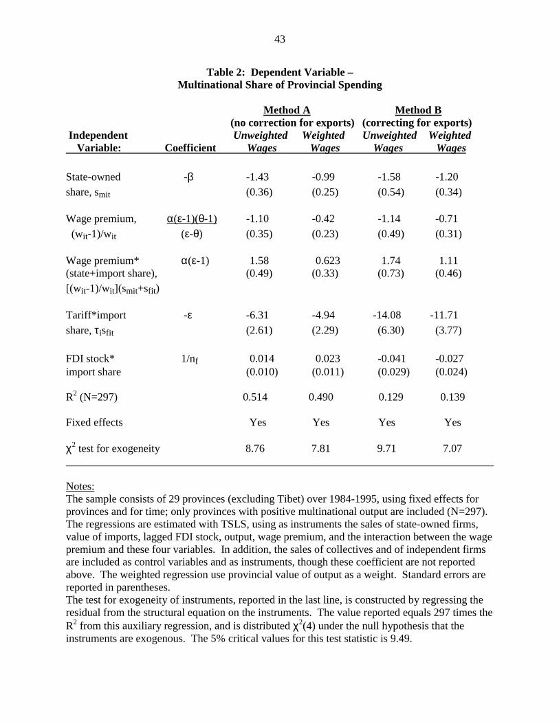
43

Table 2: Dependent Variable –Multinational Share of Provincial Spending

Method A Method B(no correction for exports) (correcting for exports)

Independent Unweighted Weighted Unweighted Weighted Variable: Coefficient Wages Wages Wages Wages

State-owned -β -1.43 -0.99 -1.58 -1.20share, smit (0.36) (0.25) (0.54) (0.34)

Wage premium, α(ε-1)(θ-1) -1.10 -0.42 -1.14 -0.71 (wit-1)/wit (ε-θ) (0.35) (0.23) (0.49) (0.31)

Wage premium* α(ε-1) 1.58 0.623 1.74 1.11(state+import share), (0.49) (0.33) (0.73) (0.46)[(wit-1)/wit](smit+sfit )

Tariff*import -ε -6.31 -4.94 -14.08 -11.71share, τisfit (2.61) (2.29) (6.30) (3.77)

FDI stock* 1/nf 0.014 0.023 -0.041 -0.027import share (0.010) (0.011) (0.029) (0.024)

R2 (N=297) 0.514 0.490 0.129 0.139

Fixed effects Yes Yes Yes Yes

χ2 test for exogeneity 8.76 7.81 9.71 7.07

Notes:The sample consists of 29 provinces (excluding Tibet) over 1984-1995, using fixed effects forprovinces and for time; only provinces with positive multinational output are included (N=297).The regressions are estimated with TSLS, using as instruments the sales of state-owned firms,value of imports, lagged FDI stock, output, wage premium, and the interaction between the wagepremium and these four variables. In addition, the sales of collectives and of independent firmsare included as control variables and as instruments, though these coefficient are not reportedabove. The weighted regression use provincial value of output as a weight. Standard errors arereported in parentheses.The test for exogeneity of instruments, reported in the last line, is constructed by regressing theresidual from the structural equation on the instruments. The value reported equals 297 times theR2 from this auxiliary regression, and is distributed χ2(4) under the null hypothesis that theinstruments are exogenous. The 5% critical values for this test statistic is 9.49.

44

Table 3: Coefficient Estimates, by Time Period

Method A Method B(no correction for exports) (correcting for exports)

Independent Unweighted Weighted Unweighted Weighted Variable: Coefficient Wages Wages Wages Wages

1984-1995 α 0.30 0.16 0.13 0.10(N=297) (0.09) (0.08) (0.03) (0.04)

β 1.43 0.99 1.58 1.20(0.36) (0.25) (0.54) (0.38)

ε 6.31 4.94 14.08 11.71(2.61) (2.30) (6.30) (3.78)

1988-1995 α 0.34 0.18 0.32 0.29(N=225) (0.15) (0.13) (0.18) (0.26)

β 1.19 0.68 1.21 1.06(0.38) (0.20) (0.32) (0.34)

ε 5.11 4.10 5.29 4.61(2.90) (2.61) (3.03) (3.57)

1990-1995 α 0.47 0.32 0.27 0.42(N=171) (0.40) (0.52) (0.13) (0.61)

β 1.03 0.45 1.19 1.06(0.38) (0.15) (0.36) (0.34)

ε 3.29 2.05 5.47 3.31(2.59) (1.78) (2.63) (3.28)

NotesComputed from the regressions reported in Table 2, but run over different time periods.

45

Table 4: Welfare Effects of Tariffs Reductions(expressed as percent of import value)

Example 1 (ε=5, θ=0.5) Example 2 (ε=10, θ=2)WTOTariffs

Direct(21)

Indirect(22)

TotalEffect

Direct(21)

Indirect(22)

TotalEffect

Beijing 0.310 2.16 -3.40 -1.24 20.40 -2.90 17.50Tianjin 0.230 0.70 -2.58 -1.88 10.29 -2.15 8.14

Include “Open Coastal Cities” or SEZLiaoning 0.170 -1.35 -0.82 -2.16 4.49 -0.76 3.73Hebei 0.217 0.83 -0.81 0.02 10.16 -0.70 9.47Shandong 0.212 1.06 -1.55 -0.48 9.90 -1.46 8.44Jiangsu 0.167 -0.08 -2.10 -2.18 5.27 -1.97 3.30Shanghai 0.122 -2.24 -2.12 -4.36 0.31 -1.86 -1.55Zhejiang 0.180 1.07 -0.95 0.11 7.19 -0.85 6.34Fujian 0.224 2.47 -4.09 -1.61 11.33 -3.63 7.70Guangdong 0.161 0.17 -5.10 -4.94 4.49 -4.83 -0.34Guangxi 0.189 -0.55 -0.78 -1.33 6.59 -0.69 5.90Hainan 0.129 -1.86 -1.18 -3.04 0.31 -1.00 -0.69

Average 0.177 -0.05 -1.95 -2.00 6.00 -1.77 4.23Do not include “Open Coastal Cities” or SEZ

Heilongjiang 0.198 -2.32 -0.35 -2.67 6.00 -0.31 5.70Jilin 0.131 -3.06 -0.39 -3.45 0.54 -0.32 0.21Inner Mongolia 0.240 -0.60 -0.43 -1.03 11.31 -0.34 10.97Shanxi 0.162 -1.64 -0.13 -1.77 3.82 -0.11 3.72Henan 0.221 1.11 -0.55 0.56 10.81 -0.48 10.33Anhui 0.181 -0.28 -0.35 -0.64 6.22 -0.31 5.91Hubei 0.146 -1.56 -0.39 -1.95 2.80 -0.35 2.45Jiangxi 0.193 -1.35 -0.40 -1.75 6.32 -0.34 5.98Hunan 0.157 -1.52 -0.34 -1.86 3.50 -0.30 3.20Guizhou 0.104 -3.08 -0.14 -3.22 -0.59 -0.11 -0.70Yunnan 0.176 -2.93 -0.25 -3.18 3.60 -0.21 3.40Sichuan 0.140 -1.78 -0.38 -2.16 2.21 -0.34 1.87Tibet 0.241 -4.46 0.00 -4.46 6.12 0.00 6.12Qinghai 0.118 -3.92 -0.03 -3.95 -0.59 -0.02 -0.61Shaanxi 0.176 -2.35 -0.42 -2.77 4.08 -0.36 3.72Gansu 0.110 -3.14 -0.18 -3.32 -0.42 -0.14 -0.56Ningxia 0.128 -3.35 -0.45 -3.81 0.25 -0.36 -0.11Xinjiang 0.069 -2.67 -0.06 -2.73 -1.43 -0.05 -1.48

Average 0.160 -2.16 -0.29 -2.45 3.59 -0.25 3.34

Notes:Other parameters used in both examples are α=0.2 and β=1. The values shown give the welfareeffects of reducing tariffs from the level shown in Table 1 to that shown above. The direct effectis calculated using (21) in the text, and the indirect effect is calculated using (22)

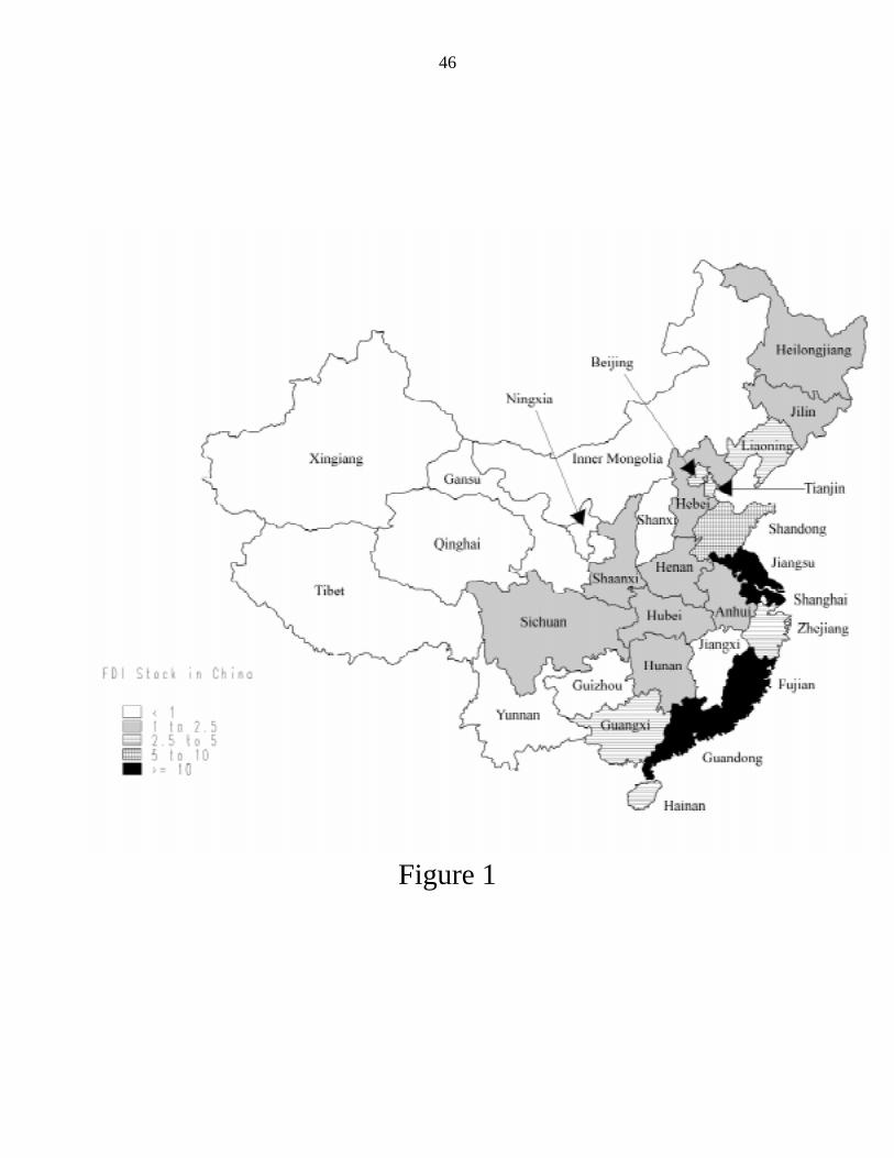
46

Figure 1

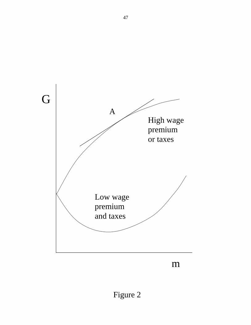
47

m

GA

High wagepremiumor taxes

Low wagepremiumand taxes

Figure 2