Embed Size (px)
Citation preview

International Trade and Job Polarization:
Evidence at the Worker Level∗
Wolfgang Keller†
University of Colorado and NBER
Hale Utar§
Bielefeld University
May 29, 2016
This paper examines the role of international trade for job polarization, the phenomenon in which employment
for high- and low-wage occupations increases but mid-wage occupations decline. With employer-employee
matched data on virtually all workers and firms in Denmark between 1999 and 2009, we use instrumental-
variables techniques and a quasi-natural experiment to show that import competition is a major cause of job
polarization. Import competition with China accounts for about 17% of the aggregate decline in mid-wage
employment. Many mid-skill workers are pushed into low-wage service jobs while others move into high-wage
jobs. The direction of movement, up or down, turns on the skill focus of workers’ education. Workers with
vocational training for a service occupation can avoid moving into low-wage service jobs, and among them
workers with information-technology education are far more likely to move into high-wage jobs than other
workers.
∗This study is sponsored by the Labor Market Dynamics and Growth Center at the University ofAarhus. Support of the Department of Economics and Business, Aarhus University and Statistics Den-mark is acknowledged with appreciation. We thank Henning Bunzel for facilitating the access to theconfidential database of Statistics Denmark and for his support, William Ridley for research assistance,Anna Salomons for sending us data, David Autor and Esther Ann Bøler for their discussions, and Su-santo Basu, Nick Bloom, Rene Boheim, Dave Donaldson, Ben Faber, Kyle Handley, Marc Muendler, Ja-gadeesh Sivadasan, Casper Thorning as well as audiences at the AEA (San Francisco), UIBE Beijing, JKULinz, LSE, ZEW Mannheim, Michigan, CESifo Munich, NBER CRIW, NBER Trade, and EIIT Purdue forhelpful comments and suggestions. The data source used for all figures and tables is Statistics Denmark.†: [email protected]. §: [email protected].

1 Introduction
By integrating many emerging economies the recent globalization has led to a major in-
crease in international trade. China, in particular, doubled its share of world merchandise
exports during the 1990s before almost tripling it again during the first decade of the 21st
century (World Bank 2016). During this globalization, labor markets in high-income coun-
tries became more polarized, with employment increases for high- and low-wage jobs at the
expense of mid-wage jobs.1 The top of Figure 1 shows job polarization in Denmark between
the years 1999 and 2009.2 The magnitudes are comparable to those documented for other,
larger economies such as the United States. This paper examines low-wage import competi-
tion as a source of job polarization, how it affects high-income countries’ labor markets, and
some of the policy issues this raises.
Understanding job polarization is paramount not only because the reason for the loss of
middle-class jobs matters but also because job polarization means inequality, which may
adversely affect the functioning of society. In particular, if trade creates inequality it may
prevent the winners and losers to agree on policies that increase total welfare–not least free
trade. Using administrative, longitudinal data on the universe of workers matched to firm
information between 1999 and 2009, we show that import competition has generated job
polarization in Denmark—it has the unique ability, we find, to explain both the decrease in
mid-wage and the increases in low- and high-wage employment.
We employ two approaches to address the key issue of causality. First, we define a worker’s
exposure to import competition according to the six-digit product category of the Dan-
ish economy in which the worker is active in the year 1999. The possible correlation of
product-level imports with domestic taste or productivity shocks is addressed by instru-
menting Denmark’s imports from China with imports from China of the same products in
1For the case of the Unites States, see Autor, Katz, and Kearney (2006, 2008), Autor and Dorn (2013);United Kingdom: Goos and Manning (2007); Germany: Spitz-Oener (2006), Dustmann, Ludsteck, andSchonberg (2009); France: Harrigan, Reshef, and Toubal (2015) and across 16 European countries, see Goos,Manning, and Salomons (2014).
2The figure on top shows smoothed employment share changes for all non-agricultural occupations at thethree digit occupation level that are ranked from low to high according to 1999 hourly wages. The extent ofjob polarization in Denmark during the early 2000s was comparable to that in the U.S. (see e.g. Autor andDorn 2013 for the years 1980-2005). The lower part summarizes the employment share changes into threebroad categories. Our definition of high-, mid-, and low-wage occupation categories is based on the mean1999 hourly wage; see section 2 for details. The right axis shows relative average wage growth between 1999and 2009 for the three wage categories.
1

-.2
-.1
0.1
.2.3
0 20 40 60 80 100Percentile100
x C
hang
e in
Em
ploy
men
t Sha
re
0.0
05.0
1R
elat
ive
wag
e gr
owth
-.02
0.0
2.0
4.0
6.0
8E
mpl
oym
ent s
hare
cha
nges
Low wage Mid wage High wage
Employment share changes Relative wage growth
Figure 1: Job Polarization in Denmark, 1999-2009
other high-income countries. Key to this identification strategy is that the main reason for
China’s export growth during the 2000s is her rising supply capacity due to higher pro-
ductivity and economic reforms (see Brandt, Hsieh, and Zhu 2008). It is then reasonable
that China’s export success in Denmark is similar to that in other high-income countries.
We augment this approach by employing two openness variables as additional instrumental
variables, the first based on transportation costs and the second capturing the importance of
retail trade channels in a product category. Second, we present evidence from a quasi-natural
experiment by studying the quota removal for textile exports as China entered the World
Trade Organization (WTO).3 Workers who manufacture narrowly defined textile products
subsequently subject to quota removals are compared to workers employed at other textile-
manufacturing firms. By yielding plausibly exogenous variation this trade liberalization is
a quasi-natural experiment for textiles that complements our instrumental-variables results
for Denmark’s entire economy.4
3We use “textiles” for short; these are goods in the textiles and clothing industries.4Earlier work employing the WTO textile quota removal includes Brambilla, Khandelwal, and Schott
(2010), Khandelwal, Schott, and Wei (2013), Bloom, Draca, and van Reenen (2016), and Utar (2014, 2015).Our instrumental variables strategy is similar in spirit to Haskel, Pereira, and Slaughter (2007) and Autor,
2
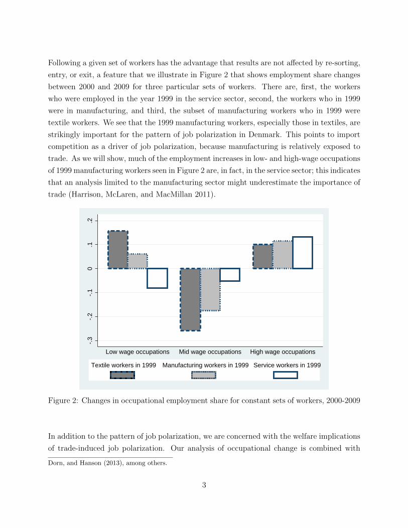
Following a given set of workers has the advantage that results are not affected by re-sorting,
entry, or exit, a feature that we illustrate in Figure 2 that shows employment share changes
between 2000 and 2009 for three particular sets of workers. There are, first, the workers
who were employed in the year 1999 in the service sector, second, the workers who in 1999
were in manufacturing, and third, the subset of manufacturing workers who in 1999 were
textile workers. We see that the 1999 manufacturing workers, especially those in textiles, are
strikingly important for the pattern of job polarization in Denmark. This points to import
competition as a driver of job polarization, because manufacturing is relatively exposed to
trade. As we will show, much of the employment increases in low- and high-wage occupations
of 1999 manufacturing workers seen in Figure 2 are, in fact, in the service sector; this indicates
that an analysis limited to the manufacturing sector might underestimate the importance of
trade (Harrison, McLaren, and MacMillan 2011).
-.3
-.2
-.1
0.1
.2
Low wage occupations Mid wage occupations High wage occupations
Textile workers in 1999 Manufacturing workers in 1999 Service workers in 1999
Figure 2: Changes in occupational employment share for constant sets of workers, 2000-2009
In addition to the pattern of job polarization, we are concerned with the welfare implications
of trade-induced job polarization. Our analysis of occupational change is combined with
Dorn, and Hanson (2013), among others.
3

evidence on the workers’ hourly wages in their new occupations. We show that not only
does import competition lead to an important shift of workers from mid- into low-wage jobs,
it also lowers these workers’ hourly wage relative to other workers in the same occupations.
On the positive side, import competition increases worker welfare because by shifting certain
mid-wage workers into high-wage jobs it accounts for about 8% of the aggregate increase in
Denmark’s high-wage employment during the sample period. Import competition matters
for welfare, both in terms of positive and negative effects, and overall we estimate that it
accounts for about 16% of the recent increase in earnings inequality in Denmark.
Given the ubiquity of job polarization in high-income countries it is natural to think about
education, whether as a way to reduce mid-wage losses or to increase the chance of mid-
to-high-wage transitions. In Denmark as in many European countries vocational training
of workers is common. Considered by some as the jewel of European education systems,
vocational training combines formal schooling with practical apprenticeships, giving an in-
termediate level of education that comes in many specific forms.
One fact to be kept in mind in the policy discussion is that vocational training is important in
industries with a high share of mid-wage jobs, both in manufacturing and in services (upper
line and lower line, respectively, Figure 3). The relatively high share of mid-wage jobs in
manufacturing on average suggests that in the past, vocational training in manufacturing has
helped workers to hold on to mid-wage jobs in this sector. Vocational training may thus be
seen as a successful defensive educational policy. However, if mid-wage manufacturing jobs
in advanced countries are vanishing, and unlikely to return (Moretti 2012), a forward-looking
educational policy will focus on training that lowers the chance of moving into low-wage,
and increases the chance for high-wage jobs—does vocational training do that? Not all, it
turns out, but some. We find that mid-skill workers trained for service vocations can avoid
moving into low-wage service jobs, and mid-skill workers trained for information-technology
vocations are far more likely to move into high-wage jobs than other workers.
In line with findings that trade with low-wage countries depresses employment and wages
in exposed parts of the economy (Autor, Dorn, and Hanson 2013, Ebenstein, Harrison,
McMillan, and Phillips 2014, Utar 2014, Hakobyan and McLaren, fortcoming, and Pierce
and Schott, forthcoming), in this paper we show that import competition from China has
adversely affected employment opportunities for much of Denmark’s labor force, explaining,
in particular, 17% of the decline in mid-wage employment. We show that import competition
has also led to substantial high-wage employment gains. To the best of our knowledge, this
4

is the first paper to show that import competition explains a major part of job polarization,
which extends the literature explaining job polarization mostly in terms of technical change
(Autor and Dorn 2013, Goos, Manning, and Salomons 2014, Michaels, Natraj, and van
Reenen 2014).5 High-wage employment gains are a manifestation of the sustained structural
effects of import competition which are the focus of this paper, in contrast to the trade
induced adjustment processes and frictions which are at the heart of the worker adjustment
literature (Dix-Carneiro 2014, Autor, Dorn, Hanson, and Song 2014, Utar 2015). We show
that import competition leads to job polarization through the shift from manufacturing
towards services (especially low-wage services). Moreover, while wage polarization, shown at
the bottom part of Figure 1, is quantitatively less important than employment polarization
in Denmark, wage effects generally reinforce the polarizing employment effects of import
competition.
Research and Development
Water Transport
Mining of Coal
Business Activities
Chemicals
Electronics
IT
Mining and Quarrying Stones, Slates, Salts
Footwear
ComputersMeasuring, Checking Eq
Extraction of Peat and OilTextiles
Hotels and Restaurants
Non-Metallic Mineral Products
64
Land Transport
Tobacco
Air Transport
Apparel
Recycling
Plastics
FoodElectrical Equipment
Supporting Transport Activities
Iron and Steel
Renting of Transport Eq and Mach
WoodFurniture
Paper
Real Estate
Publishing
Wholesale except Motor Veh.
Machinery
Motor Vehicles
Coke and Refined Petrolium
Metal Products
Retail
Other Transport Eq.
Construction
Sale and Repair of Motor Vehicles
0.2
.4.6
.8S
hare
of M
id-W
age
Wor
kers
.1 .3 .5 .7Share of Vocationally Trained Workers
ManufacturingService
Figure 3: Mid-wage workers and vocational education
Import competition is but one factor affecting employment patterns in high-wage countries,
5The leading technology explanation is that computerized machines and robots replace mid-wage earningworkers performing routine tasks (Autor, Katz, Kearney 2006, Goos and Manning 2007).
5

technical change and offshoring are others.6 Offshoring and international trade lead to wage
changes (Hummels, Jorgenson, Munch, and Xiang 2014) as well as to changes in firms’ entry,
exit, and innovation behavior (Bernard, Jensen and Schott 2006, Utar and Torres-Ruiz
2013, Utar 2014, Bloom, Draca, and van Reenen 2016). Comparing offshoring, technical
change, and import competition side-by-side, we show that both offshoring and technical
change contribute to job polarization (see Firpo, Fortin, and Lemieux 2011, and Autor,
Dorn, Hanson 2015, respectively). The key new finding is that only import competition can
explain the employment changes characteristic of job polarization in all three segments of the
wage distribution; in contrast, offshoring and technical change cannot explain high-wage and
low-wage job growth, respectively. Complementing the task analysis in Ottaviano, Peri, and
Wright (2015) and Becker and Muendler (2015), our analysis differs by performing a causal
analysis of job polarization, which also shows at the worker level that import competition
and technical change have distinct effects. We find that import competition affects mostly
workers performing manual tasks regardless of how routine intensive the tasks are.
The tri-partition of the wage distribution due to job polarization has renewed interest in
educational policies targeting the middle. In particular, even though the U.S. is said to have
a unique disdain for vocational education (Economist 2010), many in the U.S., including
President Obama, consider now some form of vocational training to be crucial (Schwartz
2013, Wyman 2015).7 By comparing vocationally trained workers with other workers, draw-
ing on virtually the entire labor force of Denmark, we bring new evidence to the table on
the efficacy of vocational training in the presence of a large labor demand shock. Key is
our ability–based on information for about 3,000 distinct educational titles–to distinguish
different forms of vocational education. Our results indicate that broadly applied vocational
education may well be ineffective in protecting workers from globalization; rather, it should
be targeted to particular skills that are evidently in high demand.
The next section lays out our empirical strategy, describes the data, and presents a num-
ber of facts on worker transitions between individual occupations in Denmark. Section 3
presents instrumental variables results on the role of trade for job polarization and assesses
its economic magnitude. Our findings are confirmed in the quasi-natural experiment of
the 2001 quota removals on Chinese textile exports in Section 4. In this context we also
show worker-task level evidence on the relationship between trade and technology in causing
6Factors such as changing labor market institutions are seen as less important, e.g., Autor (2010).7President Obama proposed making community college free to most students (Leonhardt 2015).
6

job polarization. Welfare and inequality implications of trade-induced job polarization are
analyzed in Section 5, where we also examine educational policy options with a focus on
vocational training. Section 6 provides a concluding discussion. A number of additional
results are relegated to the Online Appendix.
2 Import competition and polarization: sources of vari-
ation and measurement
2.1 Import competition
To see how the rise of low-wage countries in the global economy can lead to job polarization
in a high-wage country (Home), consider a framework in which Home has one traded and
one non-traded goods sector. Traded goods production requires intensively tasks that are
performed by workers with moderate skill levels, who are paid mid-level wages in the labor
market. An increase in productivity in the traded goods sector abroad raises foreign com-
petitiveness and exports. At Home there is an increase in the level of import competition
together with a reduction in the relative demand for mid-level wage workers. Transitions
from mid-level to other jobs will be shaped by the extent of wage adjustments as well as
any worker- or occupation- specific adjustment costs. We ask whether import competition
has caused the mid-wage employment declines and increases in both high- and low-wage
employment that are typical for job polarization.
The paper employs two complementary approaches. First, following the so-called differential
exposure approach (Goldberg and Pavcnik 2007), we study changes in import penetration
from China across six-digit product categories. At the industry-, occupation-, or regional
level the differential exposure approach has been widely applied in recent work.8 Examining
job polarization by following workers throughout the entire economy has the advantage that
the effects of globalization will not be missed even if they make themselves felt outside of
manufacturing. Second, we employ the exogenous shock of the dismantling of quotas on
Chinese textile imports in conjunction with China’s WTO accession. While the aggregate
implications of the quota removal may be limited, we can investigate the causal effect of
trade on job polarization in a quasi-experimental setting.
8See Autor, Dorn, and Hanson (2013), Kovak 2013, and Dix-Carneiro and Kovak (2015) for example.
7

Turning to the first approach, the change in import penetration from China is defined as:
∆IPCHj =
MCHj,2009 −MCH
j,1999
Cj,1999
. (1)
Here, MCHj,t denotes Denmark’s imports from China in product j and year t = {1999, 2009},
and Cj,1999 is Denmark’s consumption in initial year t = 1999, equal to production minus
exports plus imports in the six-digit product category j. We address potential endogeneity
by instrumenting the numerator of (1) with changes in imports from China in eight other
high-income countries.9 A key requirement for this strategy is that Chinese export success is
explained to a large extent by China’s increased supply capacity, which affects high-income
countries’ imports from China similarly, and that Chinese import growth is not driven by
product-level demand shocks that are common to all advanced countries.
The relatively small size of Denmark helps because, for example, it lowers the likelihood
that China’s exports target a particular Danish product. To address possible sorting in
anticipation of import changes, our instrumental variables approach utilizes consumption
levels from the year 1996. We employ two additional instrumental variables at the six-
digit level: geography-based transportation costs and a measure of the importance of retail
channels. These variables are the log average of the distance from Denmark’s import partners
using the 1996 imports as weights, and the ratio of the number of retail trading firms over
the total number of importing firms in 1996.
Figure 4 shows the change in Chinese import penetration between 1999 and 2009 across
manufacturing industries versus the share of mid-wage workers in 1999. Products belonging
to the same two-digit industry are given labels with the same color and shape. We see that
the relationship between import penetration and the share of mid-level workers varies widely
within a two-digit industry. For example, metal forming and steam generator products are
both part of the fabricated metal products industry, they both have about 50% mid-wage
worker, and yet the change in import penetration for steam generator products was much
lower than for metal forming products. What may account for these stark within-industry
differences?
9The high-income countries are Australia, Finland, Germany, Japan, Netherlands, New Zealand, Switzer-land, and USA. To construct the variable in equation (1) we employ international trade data and businessstatistics data from Statistics Denmark; the instrumental variable is based on information from the UnitedNation’s COMTRADE and Eurostat. See section 1 in the Online Appendix for details.
8

Despite their similarities, tasks performed by mid-level workers in occupations belonging to
the same two-digit industry can in fact be quite different, and so can be worker exposure
to import competition. Take “Fibre-preparing-, spinning-, and winding-machine operators”
(textile machine operators for short) and “Industrial robot operators”, for example, both
four-digit occupations of the International Standard Classification of Occupations (ISCO,
class 8261 and 8170, respectively).10 Workers in both occupations make typically mid-level
wages, and yet textile machine operators will be more negatively affected by rising import
competition compared to industrial robot operators; the latter might actually experience
improved employment prospects due to skill upgrading.11 We account for these differences
0.2
.4.6
.81
Sha
re o
f Mid
-wag
e W
orke
rsin
199
9
0 .1 .2 .3Change of Chinese Import Penetration
Food Tobacco Textiles Apparel
Footwear Wood Paper Publishing
Petroleum Chemicals Plastics Non-Metallic Mineral Products
Iron and Steel Metal Products Machinery Computers
Electrical Equipment Electronics Measuring, Checking Eq. Motor Vehicles
Transport Eq. Furniture
Figure 4: Mid-wage workers and import penetration from China
by including occupational fixed effects at the two- and four-digit level in the analysis.12
Furthermore, we exploit the employer-employee link to capture technology differences in
10Other examples of four-digit occupations include silk-screen textile printers, textile pattern makers, tai-lors, bleaching machine operators, stock clerks, data entry operators, bookkeepers, accountants, secretaries,and sewing machine operators.
11Denmark is among the countries with the highest increase in robotization during 1993-2007 (Graetz andMichaels 2015).
12More than four hundred different occupations are distinguished in our analysis.
9
more than six hundred product categories proxied by the share of information-technology
educated workers. In addition, we account for the quality level in manufacturing activity
using the wage share of vocationally educated workers in the total wage bill. We also include
two-digit industry fixed effects to avoid capturing differences in growth of Chinese imports
across industries due to broad technological differences. As a result, we are not capturing
Chinese import growth due to the potentially disproportional effect of a decline in the costs
of offshoring or automatization across broader industries.
Our second definition of exposure to import competition exploits variation at the worker level
due to a specific policy change, the removal of Multi-fibre Arrangement (MFA) quotas for
China. The entry of China in December 2001 into the WTO meant the removal of binding
quantitative restrictions on China’s exports to countries of the European Union (EU); it
triggered a surge in textile imports in Denmark during the years 2002 to 2009, and prices
declined (Utar 2014). This increase in import competition is plausibly exogenous because
Denmark did not play a major part in negotiating the quotas or their removal, which was
managed at the EU level and finalized in the year 1995. Moreover, the sheer magnitude of
the increase in imports after the quota removal was unexpected, and in part driven by the
allocative efficiency gains in China (Khandelwal, Schott, and Wei, 2013).
We implement this approach by identifying all firms that in 1999 produce narrowly defined
goods – e.g., “Shawls and scarves of silk or silk waste” – in Denmark that are subject to
the MFA quota removal for China. This is our treated group of firms. The control group of
firms with similar characteristics can be constructed because within broad product categories
the quotas did not protect all goods. We then employ the employer-employee link provided
by Statistics Denmark to obtain two sets of workers: a treatment and a control set. In
the year 1999, about half of the textile and clothing workers are exposed to rising import
competition. This setting affords us a way to strengthen the instrumental variables evidence
with a quasi-natural experiment. Section 2 in the Online Appendix gives more information
on the quota removal.
2.2 The Danish labor market
Recent work on Denmark’s labor market, including Bagger, Christensen, and Mortensen
(2014), Hummels, Jorgenson, Munch, and Xiang (2014), Utar (2015), and Groes, Kircher,
and Manovskii (2015), indicates that the country is a good candidate for examining job
10

polarization. In contrast to many continental European economies there are few barriers to
worker movements between jobs in Denmark. Turnover as well as average worker tenure is
comparable to the Anglo-Saxon labor market model (in 1995, average tenure in Denmark
was 7.9 years, comparable to 7.8 in the UK). Hiring and firing costs are low in Denmark.
This is confirmed by more recent international comparisons: for example, in the 2013 Global
Competitiveness report, Denmark and the US are similarly ranked as 6th and 9th respectively
in terms of flexibility of hiring and firing regulations.
The flexibility in terms of firing and hiring practices is combined with a high level of publicly
provided social protection. Most Danish workers participate in centralized wage bargaining,
which tends to reduce the importance of wages in the labor market adjustment process.
However, in recent years decentralization in wage determination has increased wage disper-
sion (Eriksson and Westergaard-Nielsen 2009). While we find that occupational shifts are
central to explaining polarization in the Danish labor market, our earnings and hourly wage
results are consistent with significant wage effects in Denmark in response to globalization,
as documented by Hummels, Jorgenson, Munch, and Xiang (2014).
2.3 Worker- and firm data
The main database used in this study is the Integrated Database for Labor Market Research
of Statistics Denmark, which contains administrative records on individuals and firms in
Denmark.13 We have annual information on all persons of age 15 to 70 residing in Denmark
with a social security number, information on all establishments with at least one employee
in the last week of November of each year, as well as information on all jobs that are active
in that same week. These data files have been complemented with firm-level data and
international transactions to assess exposure to import competition, as well as information
on domestic production which we employ in the quota removal analysis.
The worker information includes annual salary, hourly wage, industry code of primary em-
ployment, education level, demographic characteristics (age, gender and immigration status),
and occupation of primary employment.14 Of particular interest is the information on work-
ers’ occupation. Occupational codes matter in Denmark because they influence earnings due
13See Bunzel (2008) and Timmermans (2010) for more information.14Employment status is based on the last week in November of each year. Thus our results will not be
influenced by short-term unemployment spells or training during a year as long as the worker has a primaryemployment in the last week of November of each year.
11

to the wage determination system. Because employers and labor unions pay close attention
to occupational codes, data quality is high compared to other countries.15 As noted above,
occupation codes are generally given at the four-digit level of the ISCO-88 classification
which allows us to distinguish more than four hundred detailed occupations.
Table 1: Summary Statistics, Economy-wide Sample (n=900,329)
Mean Standard
DeviationPanel A. Outcome Variables
Cumulative Years of Employment in High Wage Jobs (2000-2009) 2.638 3.689Cumulative Years of Employment in Mid Wage Jobs (2000-2009) 3.581 3.755Cumulative Years of Employment in Low Wage Jobs (2000-2009) 1.281 2.457
Panel B. Characteristics of Workers in 1999Age 34.093 8.852Female 0.339 0.473Immigrant 0.045 0.208College Educated 0.176 0.381Vocational School Educated 0.436 0.496At most High School 0.377 0.485Years of Experience in the Labor Market 12.868 6.205History of Unemployment 1.025 1.716Log Hourly Wage 5.032 0.448High Wage Occupation 0.265 0.441Mid Wage Occupation 0.509 0.500Low Wage Occupation 0.194 0.395Union Membership 0.762 0.426
Notes: Variables Female, Immigrant, Union Membership, Unemployment Insurance (UI) Mem-
bership, High Wage, Mid Wage and Low Wage Occupations, College Educated, Vocational School
Educated and At most High School are worker-level indicator variables. History of Unemployment
is the summation of unemployment spells of worker i until 1999 (expressed in years). Values are
reported throughout the paper in 2000 Danish Kroner.
Our sample of n = 900,329 workers are all who were between 18 and 50 years old in 1999
and employed in a firm operating in the non-agricultural private sector for which Statistics
Denmark collects firm-level accounting data. By holding constant this sample of workers
and follow them as they change jobs and sectors, our results are not affected by factors that
lead to entry or exit of workers, including immigration.16 The age constraint ensures that
15Groes, Kircher, and Manovskii (2015) emphasize this point.16For example, as a result of the increase in refugees in Denmark starting in the mid-1990s, the employment
12

workers are typically active in the labor market throughout the sample period, and firm-level
accounting information is needed for a number of covariates. As of base year 1999, workers
were employed in a wide range of industries, including mining, manufacturing, wholesale
and retail trade, hotels and restaurants, transport, storage and communication, as well as
real estate, renting and business activities.17 As in most high-income countries, the sectoral
composition of the sample during this time changed from manufacturing (going from 33%
of the sample in 1999 to 20% by 2009) towards services.
Following the literature on job polarization we distill the U-shaped pattern into changes
for three separate groups, called low-, mid-level, and high-wage workers (Autor 2010, Goos,
Manning, and Salomons 2014). We form these groups based on the median wage paid
in an occupation in Denmark for the year 1999.18 The high-wage occupations comprise
of managerial, professional, and technical occupations. Mid-wage occupations are clerks,
craft and related trade workers, as well as plant and machine operators and assemblers.
Finally, low-wage occupations include service workers, shop and market sales workers, as
well as workers employed in elementary occupations. Descriptive statistics for the sample
are reported in Table 1. Panel A provides information on the employment trajectories of the
workers between 2000 and 2009. On average across all workers, the number of years spent
in mid-wage occupations was about 3.6 years. This is one of our outcomes variables, defined
as
MIDei =
2009∑t=2000
Empmit , (2)
where Empmit is an indicator variable that takes the value of one if worker i has held a primary
job in mid-level wage occupations in year t ∈ T (T = {2000, ..., 2009}). The variable MIDei
ranges from a maximum of 10 years for a 1999 mid-wage worker who has been employed in
mid-wage occupations throughout the years 2000 to 2009, to a minimum of 0 for an 1999
share of Non-European Union immigrants increased from 2.5 to 4.5 % until the mid-2000s; see Foged andPeri (2016) for a study of the impact of refugees on native worker outcomes in Denmark.
17Sectors that are not included as initial employment of workers in the sample are mainly public admin-istration, education, health, and a wide range of small personal and social service providers. Education andhealth sectors in Denmark are to a large extent publicly owned. We have also employed a larger sampleincluding the public sector with about 1.5 million observations, finding that this does not yield importantadditional insights.
18We rank occupations at the one-digit level for full-time workers (see Table A-1). An advantage ofclassifying major occupations is that the mapping of occupations into high-, mid-, and low wage categoriesdoes not change throughout the sample period. Employing the classification of Goos, Manning, Salomons(2014) based on the 1993 wages at the two-digit ISCO across European countries including Denmark leadsto very similar results.
13
high- or low-wage worker who never had a spell in mid-wage jobs. MIDei takes higher values
if worker i was employed in a mid-wage occupation in 1999 and stayed in his or her job, or
if worker i was initially employed in high- or low-wage occupations but transitioned into a
mid-wage occupation relatively early. Occupational change within the category of mid-wage
occupations is not picked up by this variable. Analogously, we define LOW ei and HIGHe
i
as the cumulative low-wage and high-wage employment of worker i between the years 2000
and 2009.
The percentage of workers with college education is 18%, 44% of workers have formal vo-
cational training, and the remaining 38% workers have at most high school education. In
Denmark vocational education is provided by the technical high schools (after 9 years of
mandatory schooling) and involves several years of training with both schooling and appren-
ticeships. As typical of many European countries our sample has a relatively high share of
vocationally-trained workers.19
For the textile worker sample that will be employed in the quota removal analysis, summary
statistics are shown in Table 2. We focus on workers who are of working age throughout
our sample period, about 10.5 thousand workers.20 Compared to the economy as a whole,
as typical of manufacturing in general, mid-wage occupations are relatively more important
(66% of textile workers hold mid-wage occupations in 1999).
19The shares of college, vocational, and at most high school education for Denmark as a whole in 1999 arequite similar to those in our sample; the former are 25%, 43%, and 32%, respectively.
20Since this sample is smaller our age limits are less conservative. Workers are between 17 and 57 yearsold in 1999, which ensures that they will typically be active in the labor market between 2002 and 2009.
14
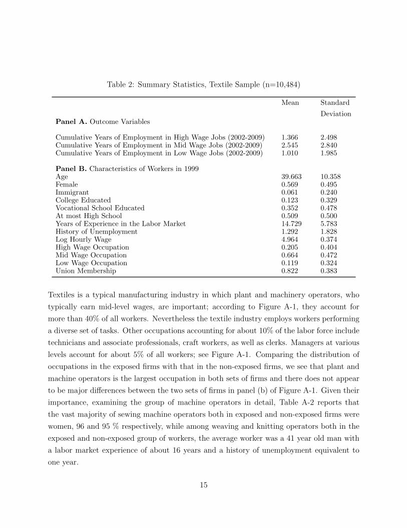
Table 2: Summary Statistics, Textile Sample (n=10,484)
Mean Standard
DeviationPanel A. Outcome Variables
Cumulative Years of Employment in High Wage Jobs (2002-2009) 1.366 2.498Cumulative Years of Employment in Mid Wage Jobs (2002-2009) 2.545 2.840Cumulative Years of Employment in Low Wage Jobs (2002-2009) 1.010 1.985
Panel B. Characteristics of Workers in 1999Age 39.663 10.358Female 0.569 0.495Immigrant 0.061 0.240College Educated 0.123 0.329Vocational School Educated 0.352 0.478At most High School 0.509 0.500Years of Experience in the Labor Market 14.729 5.783History of Unemployment 1.292 1.828Log Hourly Wage 4.964 0.374High Wage Occupation 0.205 0.404Mid Wage Occupation 0.664 0.472Low Wage Occupation 0.119 0.324Union Membership 0.822 0.383
Textiles is a typical manufacturing industry in which plant and machinery operators, who
typically earn mid-level wages, are important; according to Figure A-1, they account for
more than 40% of all workers. Nevertheless the textile industry employs workers performing
a diverse set of tasks. Other occupations accounting for about 10% of the labor force include
technicians and associate professionals, craft workers, as well as clerks. Managers at various
levels account for about 5% of all workers; see Figure A-1. Comparing the distribution of
occupations in the exposed firms with that in the non-exposed firms, we see that plant and
machine operators is the largest occupation in both sets of firms and there does not appear
to be major differences between the two sets of firms in panel (b) of Figure A-1. Given their
importance, examining the group of machine operators in detail, Table A-2 reports that
the vast majority of sewing machine operators both in exposed and non-exposed firms were
women, 96 and 95 % respectively, while among weaving and knitting operators both in the
exposed and non-exposed group of workers, the average worker was a 41 year old man with
a labor market experience of about 16 years and a history of unemployment equivalent to
one year.
15

1999 2001 2003 2005 2007 20090
10
20
30
40
50
60
70
80
90
100
Year
Per
cent
Exposed, staying as machine operatorNon−Exposed, staying as machine operatorExposed, transitioning to personal servicesNon−Exposed, transitioning to personal services
Figure 5: Occupational Transition Probabilities of Textile Machine Operators by ExposureTo Competition
If import competition causes job polarization, mid-wage employment reductions and high-
and low-wage increases must be relatively pronounced for workers who are employed in 1999
in firms that subsequently are affected by the quota removal. Figure 5 provides some initial
evidence on this by comparing the job transitions of treated and untreated machine operators
and assemblers (ISCO 82; machine operators for short). Consider first the hollowing out of
mid-wage employment. Because we start with the universe of machine operators in 1999
and do not include post-1999 entrants, the two upper lines in Figure 5 start at 100% and
slope downward over time. The chief observation is that the rate at which machine operators
leave their occupation in exposed firms is considerably higher than the rate at which they
leave it in non-exposed firms. To be sure, the pattern of Figure 5 suggests that demand for
machine operator services has declined for a number of reasons (such as technical change).
At the same time, in 2009 only about 15% of the exposed machine operators are in that same
occupation, which compares to about 23% machine operators that remain in their original
occupations conditional on not being exposed to rising import competition.
16

Turning to increases in low-wage employment, the two lower lines in Figure 5 give the
cumulative probabilities of machine operator transitions to personal and protective services
(ISCO 51). This is a low-wage occupation that includes the organization and provision
of travel services, housekeeping, child care, hairdressing, funeral arrangements, as well as
protection of individuals and personal property. Occupations such as these have played a
major role in the polarization of the U.S. labor market (Autor and Dorn 2013). Figure 5
shows that the movement of exposed machine operators into personal and protective service
jobs is considerably more pronounced than for non-exposed machine operators. By the year
2009, about 9% of the original exposed machine operators are in the personal and protective
service occupation, compared to about 6% of the non-exposed machine operators. This
evidence is in line with findings of a recent strengthening of trade effects in larger and less
open economies such as the U.S. (Autorn, Dorn, and Hanson 2015). Consistent with job
polarization, workers exposed to rising import competition move relatively strongly from
mid-wage into low-wage occupations. It is also interesting that the extent to which exposed
workers move more noticeably away from mid-wage and towards low-wage jobs than non-
exposed workers is quite similar (about 50%). The movement away from mid-wage and
towards low-wage jobs seems to be driven by the same factor: namely, import competition.
A similar figure for high-wage occupations (not shown) suggests that exposed workers move
also more strongly than non-exposed workers into high-wage occupations.
If a given exposed worker leaves his or her occupation the worker will typically take a job
in either a high or a low-wage occupation, not in both. In our sample with more than
900,000 observations, more than 95% of the 1999 mid-wage workers either stay in that wage
category or move either up or down for any amount of time during 2000-2009. Of all workers
that had mid-wage occupations in 1999, 22% had high-wage employment and 21% had low-
wage employment during the years 2000-2009. What about these figures for 1999 mid-wage
workers exposed to rising import competition? For those, the share of workers with high-
wage employment during 2000-2009 is 19%, whereas the share with low-wage employment
during the same time is 25%.21 Thus import competition is associated with a decline in
transitions to high-wage occupations and an increase in transitions to low-wage occupations.
21Strongly exposed is defined here as a worker at the 90th percentile in terms of Chinese import competi-tion.
17
3 Import competition causes economy-wide polariza-
tion
3.1 Chinese Imports and the Decline in Mid-Wage Jobs
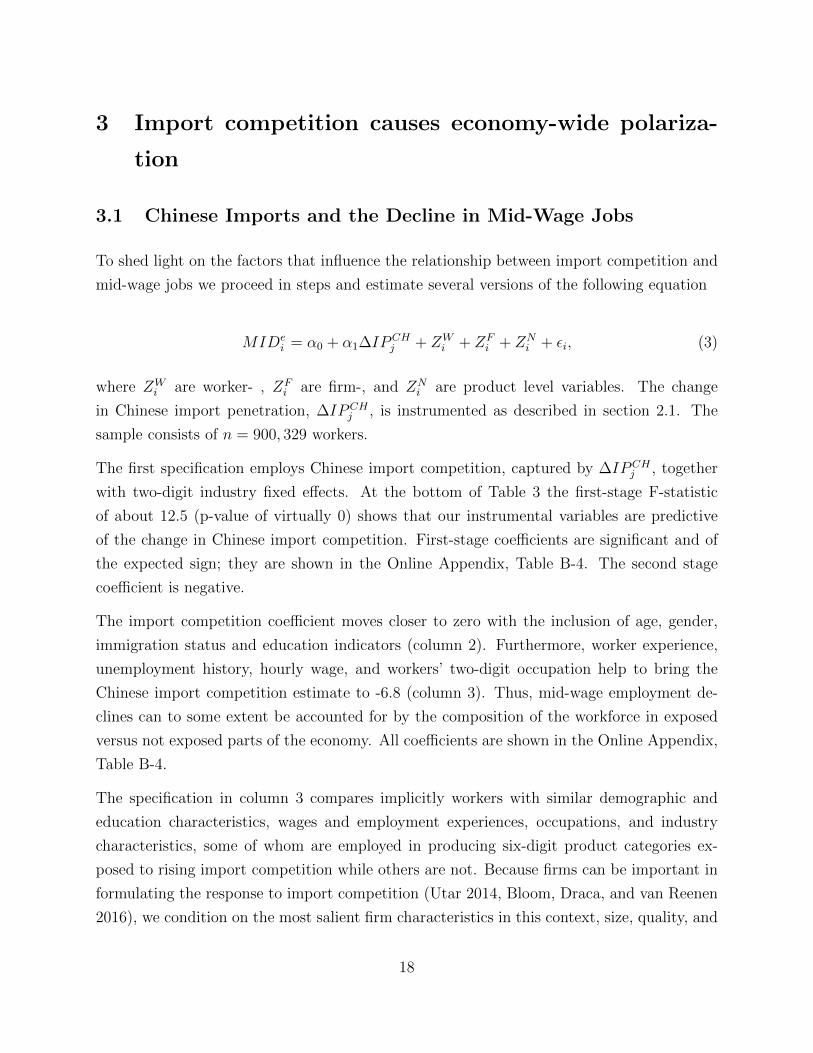
To shed light on the factors that influence the relationship between import competition and
mid-wage jobs we proceed in steps and estimate several versions of the following equation
MIDei = α0 + α1∆IP
CHj + ZW
i + ZFi + ZN
i + εi, (3)
where ZWi are worker- , ZF
i are firm-, and ZNi are product level variables. The change
in Chinese import penetration, ∆IPCHj , is instrumented as described in section 2.1. The
sample consists of n = 900, 329 workers.
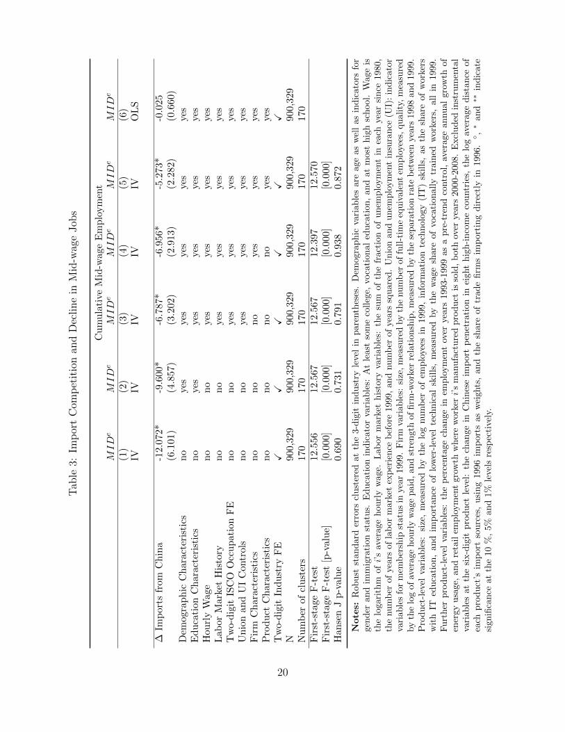
The first specification employs Chinese import competition, captured by ∆IPCHj , together
with two-digit industry fixed effects. At the bottom of Table 3 the first-stage F-statistic
of about 12.5 (p-value of virtually 0) shows that our instrumental variables are predictive
of the change in Chinese import competition. First-stage coefficients are significant and of
the expected sign; they are shown in the Online Appendix, Table B-4. The second stage
coefficient is negative.
The import competition coefficient moves closer to zero with the inclusion of age, gender,
immigration status and education indicators (column 2). Furthermore, worker experience,
unemployment history, hourly wage, and workers’ two-digit occupation help to bring the
Chinese import competition estimate to -6.8 (column 3). Thus, mid-wage employment de-
clines can to some extent be accounted for by the composition of the workforce in exposed
versus not exposed parts of the economy. All coefficients are shown in the Online Appendix,
Table B-4.
The specification in column 3 compares implicitly workers with similar demographic and
education characteristics, wages and employment experiences, occupations, and industry
characteristics, some of whom are employed in producing six-digit product categories ex-
posed to rising import competition while others are not. Because firms can be important in
formulating the response to import competition (Utar 2014, Bloom, Draca, and van Reenen
2016), we condition on the most salient firm characteristics in this context, size, quality, and
18

the extent to which workers separate from their firms. These firm variables do not change
the import competition estimate much (column 4).
Mid-wage employment is likely to be affected by the adoption of new information and commu-
nication technologies (ICTs). To capture this we include the share of information technology-
educated workers for each of the roughly 600 product categories. Furthermore, we add the
wage share of vocationally trained workers. The coefficient for Chinese import competition
is now estimated at about -5.3 (column 5). This is less than half the size of the effect in
column 1, underlining the importance of the worker-, firm-, and product variables that we
employ.
The performance of the instrumental variables does not change much with the inclusion of
worker, firm, and product-level variables. In particular, the first-stage F-statistic is similar,
and the over-identification tests present no evidence that the instrumental variables are not
valid. The final column in Table 3 shows OLS results for comparison. The Chinese imports
variable has a negative point estimate close to zero. This is consistent with the hypothesis
that import demand from China is positively correlated with industry demand shocks, and
failing to account for this correlation, the OLS estimate is upwardly biased.
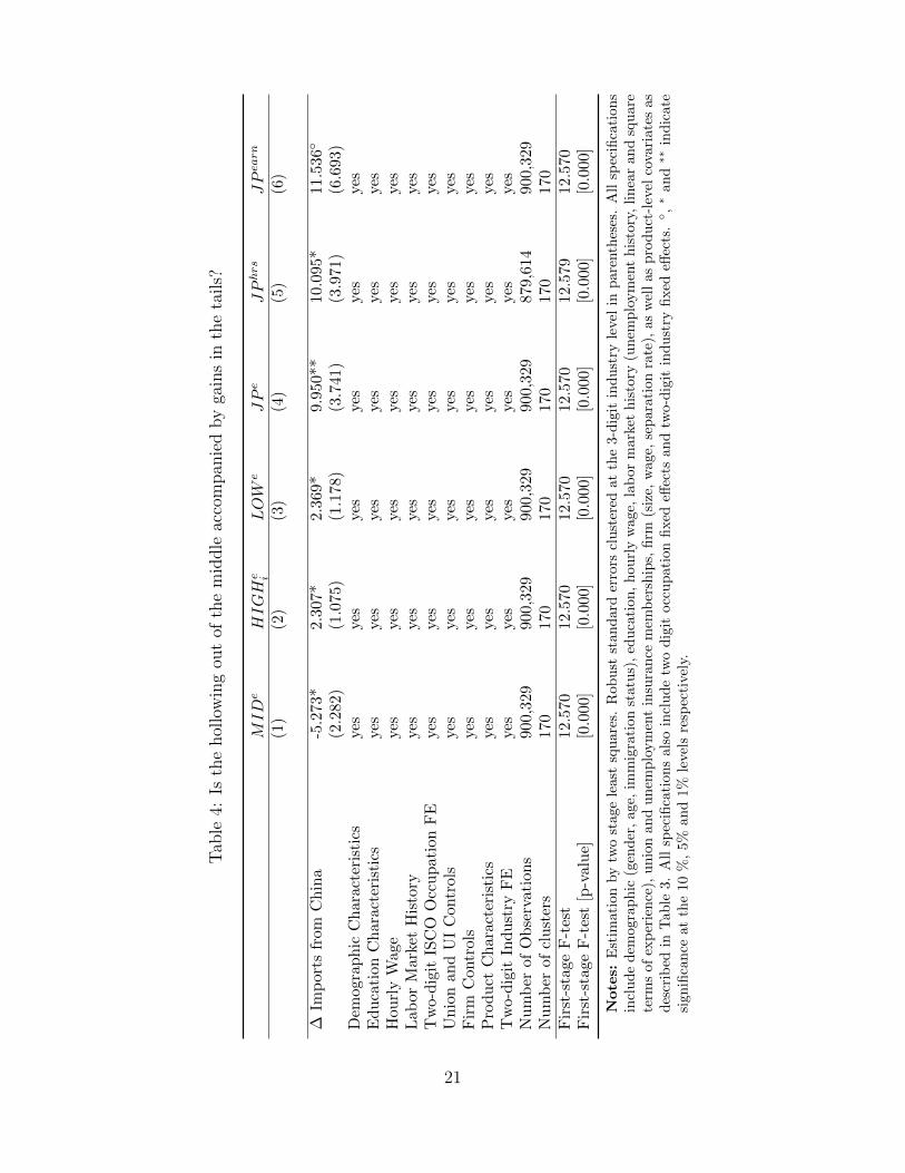
3.2 Can trade explain the U-shaped job polarization pattern?
This section asks whether rising import competition leads to employment increases in the
high- and low-wage tails of the distribution. Without these increases one cannot conclude
that import competition causes job polarization.
We begin with employment in high-wage occupations. The dependent variable is HIGHei ,
the cumulative number of years that worker i has worked in high-wage occupations during
2000-2009. Otherwise the specification is identical to the regression of Table 3, column 5
(presented again for convenience in Table 4). We see that workers exposed to rising Chinese
import competition have more employment in high-wage jobs than otherwise similar workers
that are not exposed. We also see that workers exposed to import competition have more
low-wage employment than not exposed workers (column 3). Overall the results show that
rising import competition from China has caused job polarization in Denmark.
19
Tab
le3:
Imp
ort
Com
pet
itio
nan
dD
ecline
inM
id-w
age
Job
s
Cu
mu
lati
veM
id-w
age
Em
plo
ym
ent
MID
eM
ID
eM
ID
eM
ID
eM
ID
eM
ID
e
(1)
(2)
(3)
(4)
(5)
(6)
IVIV
IVIV
IVO
LS
∆Im
por
tsfr
om
Ch
ina
-12.
072*
-9.6
00*
-6.7
87*
-6.9
56*
-5.2
73*
-0.0
25(6
.101
)(4
.857
)(3
.202
)(2
.913
)(2
.282
)(0
.660
)D
emog
rap
hic
Ch
ara
cter
isti
csn
oye
sye
sye
syes
yes
Ed
uca
tion
Ch
arac
teri
stic
sn
oye
sye
syes
yes
yes
Hou
rly
Wage
no
no
yes
yes
yes
yes
Lab
orM
arke
tH
isto
ryn
on
oye
sye
sye
syes
Tw
o-d
igit
ISC
OO
ccu
pat
ion
FE
no
no
yes
yes
yes
yes
Un
ion
an
dU
IC
ontr
ols
no
no
yes
yes
yes
yes
Fir
mC
har
acte
rist
ics
no
no
no
yes
yes
yes
Pro
du
ctC
har
acte
rist
ics
no
no
no
no
yes
yes
Tw
o-d
igit
Ind
ust
ryF
EX
XX
XX
XN
900,
329
900,
329
900,
329
900,
329
900,
329
900,
329
Nu
mb
erof
clu
ster
s17
017
017
017
017
017
0F
irst
-sta
ge
F-t
est
12.5
5612
.567
12.5
6712
.397
12.5
70F
irst
-sta
ge
F-t
est
[p-v
alu
e][0
.000
][0
.000
][0
.000
][0
.000
][0
.000
]H
an
sen
Jp
-valu
e0.
690
0.73
10.
791
0.93
80.
872
Note
s:R
obu
stst
and
ard
erro
rscl
ust
ered
at
the
3-d
igit
indu
stry
leve
lin
pare
nth
eses
.D
emogra
ph
icva
riab
les
are
age
as
wel
las
ind
icato
rsfo
rge
nd
eran
dim
mig
rati
onst
atu
s.E
du
cati
onin
dic
ato
rva
riab
les:
At
least
som
eco
lleg
e,vo
cati
on
al
edu
cati
on
,an
dat
most
hig
hsc
hool.
Wage
isth
elo
gari
thm
ofi’
sav
erag
eh
ourl
yw
age.
Lab
or
mark
eth
isto
ryva
riab
les:
the
sum
of
the
fract
ion
of
un
emp
loym
ent
inea
chye
ar
sin
ce1980,
the
nu
mb
erof
year
sof
lab
orm
arke
tex
per
ien
ceb
efore
1999,
an
dnu
mb
erof
years
squ
are
d.
Un
ion
an
du
nem
plo
ym
ent
insu
ran
ce(U
I):
ind
icato
rva
riab
les
for
mem
ber
ship
stat
us
inye
ar19
99.
Fir
mva
riab
les:
size
,m
easu
red
by
the
nu
mb
erof
full
-tim
eeq
uiv
ale
nt
emp
loye
es,
qu
ali
ty,
mea
sure
dby
the
log
ofav
erag
eh
ourl
yw
age
pai
d,
and
stre
ngth
of
firm
-work
erre
lati
on
ship
,m
easu
red
by
the
sep
ara
tion
rate
bet
wee
nye
ars
1998
an
d1999.
Pro
du
ct-l
evel
vari
able
s:si
ze,
mea
sure
dby
the
log
nu
mb
erof
emp
loye
esin
1999,
info
rmati
on
tech
nolo
gy
(IT
)sk
ills
,as
the
share
of
work
ers
wit
hIT
edu
cati
on,
and
imp
orta
nce
oflo
wer
-lev
elte
chn
ical
skil
ls,
mea
sure
dby
the
wage
share
of
voca
tion
all
ytr
ain
edw
ork
ers,
all
in1999.
Fu
rth
erp
rod
uct
-lev
elva
riab
les:
the
per
centa
ge
chan
ge
inem
plo
ym
ent
over
years
1993-1
999
as
ap
re-t
ren
dco
ntr
ol,
aver
age
an
nu
al
gro
wth
of
ener
gyu
sage
,an
dre
tail
emp
loym
ent
grow
thw
her
ew
ork
eri’
sm
anu
fact
ure
dp
rod
uct
isso
ld,
both
over
years
2000-2
008.
Excl
ud
edin
stru
men
tal
vari
able
sat
the
six-d
igit
pro
du
ctle
vel:
the
change
inC
hin
ese
imp
ort
pen
etra
tion
inei
ght
hig
h-i
nco
me
cou
ntr
ies,
the
log
aver
age
dis
tan
ceof
each
pro
du
ct’s
imp
ort
sou
rces
,u
sin
g19
96im
port
sas
wei
ghts
,an
dth
esh
are
of
trad
efi
rms
imp
ort
ing
dir
ectl
yin
1996.◦ ,∗
an
d∗∗
ind
icate
sign
ifica
nce
atth
e10
%,
5%an
d1%
leve
lsre
spec
tive
ly.
20
Tab
le4:
Isth
ehol
low
ing
out
ofth
em
iddle
acco
mpan
ied
by
gain
sin
the
tails?
MID
eHIGH
e iLOW
eJP
eJP
hrs
JP
earn
(1)
(2)
(3)
(4)
(5)
(6)
∆Im
por
tsfr
om
Ch
ina
-5.2
73*
2.30
7*2.
369*
9.95
0**
10.0
95*
11.5
36◦
(2.2
82)
(1.0
75)
(1.1
78)
(3.7
41)
(3.9
71)
(6.6
93)
Dem
ogr
aph
icC
hara
cter
isti
csyes
yes
yes
yes
yes
yes
Ed
uca
tion
Ch
ara
cter
isti
csye
sye
sye
syes
yes
yes
Hou
rly
Wag
eye
sye
sye
syes
yes
yes
Lab
orM
ark
etH
isto
ryyes
yes
yes
yes
yes
yes
Tw
o-d
igit
ISC
OO
ccu
pat
ion
FE
yes
yes
yes
yes
yes
yes
Un
ion
and
UI
Contr
ols
yes
yes
yes
yes
yes
yes
Fir
mC
ontr
ols
yes
yes
yes
yes
yes
yes
Pro
du
ctC
hara
cter
isti
csyes
yes
yes
yes
yes
yes
Tw
o-d
igit
Ind
ust
ryF
Eye
sye
syes
yes
yes
yes
Nu
mb
erof
Ob
serv
ati
on
s90
0,32
990
0,32
990
0,32
990
0,32
987
9,61
490
0,32
9N
um
ber
of
clu
ster
s17
017
017
017
017
017
0F
irst
-sta
ge
F-t
est
12.5
7012
.570
12.5
7012
.570
12.5
7912
.570
Fir
st-s
tage
F-t
est
[p-v
alu
e][0
.000
][0
.000
][0
.000
][0
.000
][0
.000
][0
.000
]
Note
s:E
stim
atio
nby
two
stag
ele
ast
squ
ares
.R
ob
ust
stan
dard
erro
rscl
ust
ered
at
the
3-d
igit
ind
ust
ryle
vel
inp
are
nth
eses
.A
llsp
ecifi
cati
on
sin
clu
de
dem
ogra
ph
ic(g
end
er,
age,
imm
igra
tion
statu
s),
edu
cati
on
,h
ou
rly
wage,
lab
or
mark
ethis
tory
(un
emp
loym
ent
his
tory
,li
nea
ran
dsq
uare
term
sof
exp
erie
nce
),u
nio
nan
du
nem
plo
ym
ent
insu
ran
cem
emb
ersh
ips,
firm
(siz
e,w
age,
sep
ara
tion
rate
),as
wel
las
pro
du
ct-l
evel
cova
riate
sas
des
crib
edin
Tab
le3.
All
spec
ifica
tion
sal
soin
clu
de
two
dig
itocc
up
ati
on
fixed
effec
tsan
dtw
o-d
igit
ind
ust
ryfi
xed
effec
ts.◦ ,∗
an
d∗∗
ind
icate
sign
ifica
nce
atth
e10
%,
5%an
d1%
leve
lsre
spec
tive
ly.
21

To assess economic magnitudes we compare two workers, one at the 10th and the other at the
90th percentile of exposure to import competition. The difference in the change in Chinese
import penetration for these workers is 0.037. With a coefficient of about -5.3 in column
1, a highly exposed worker has typically just under 0.2 years of mid-wage employment less
than the typical not exposed worker.22 The coefficients in columns 2 and 3 translate into
about 0.09 years more of high-wage and low-wage employment each. Because the sum of the
trade-induced employment effects across all three wage categories is close to zero, movements
outside of the labor market (long-term unemployment, training) do not affect these results
much.
To put this in perspective, a worker with a bad unemployment history for example has
usually 0.4 years less mid-wage employment between 2000 and 2009 than a worker with a
good unemployment history, and a 47 years old worker has typically 0.5 years less mid-
wage employment than a 22 years old worker. A worker employed in a large firm (500 or
more employees) has 0.06 years more high-wage employment over ten years than a worker
employed in a smaller firm with five employees. These figures suggest that globalization has
sizable effects.
While the finding of negative globalization effects for some workers is not new, the result that,
through the transitioning of workers into higher-wage occupations as well as into low-wage
occupations, import competition leads to job polarization is, to the best of our knowledge,
novel. The benefits from moving into high-wage occupations are independent from other
positive welfare effects of globalization, for example through lower goods prices.
To facilitate some of the exposition in the following, we define a polarization measure that
simultaneously captures employment increases in the tails and decreases in the middle. Let
JP ei be defined as the sum of years of employment in high- and low-wage occupations, minus
years employed in mid-wage occupations, over the period 2000 to 2009:
JP ei = HIGHe
i + LOW ei −MIDe
i , ∀i . (4)
This variable gives equal weight to employment increases in the tails and decreases in the
middle. By construction, the coefficient on Chinese imports in the regression with JP ei as the
dependent variable is equal to the sum of the absolute values of the coefficients with HIGH,
22If we focus on the 90/10 exposure difference for manufacturing workers, the effect becomes larger, namely0.42 years.
22

MID, and LOW as the dependent variables (see Table 4, columns 1 to 4). Analogously, we
define an hours worked variable as
JP hrsi = HIGHhrs
i + LOW hrsi −MIDhrs
i , ∀i (5)
where HIGHhrsi is the number of hours that worker i was employed in high-wage occupations
during the period 2000-2009, relative to initial annual hours worked by worker i; MID and
LOW are defined analogously. Employing this measure we see that the impact of Chinese
import competition on hours worked is quite similar to that for years of employment (column
5, compared to 4). This suggests that the more permanent movements captured by the years
of employment variable describe the job polarization experience quite well.
By analyzing polarization in terms of years and hours of employment we have so far focused
on quantity effects. Turning to earnings polarization, we define:
JP earni = HIGHearn
i + LOW earni −MIDearn
i , ∀i. (6)
Here, HIGHearni is the earnings of worker i in high-wage occupations over the years 2000-
2009, relative to i’s annual earnings in 1999; LOW earni and MIDearn
i are defined analogously.
Employing the same instrumental-variables approach as before, the positive coefficient indi-
cates that rising import competition from China has caused earnings polarization in Denmark
(column 6). We also see that the coefficient in the earnings regression is somewhat higher
than in the employment regressions (columns 5, 6). Wage growth for exposed workers in the
sample has been relatively low for workers in the middle of the distribution, consistent with
the overall wage growth pattern in Denmark of Figure 1.
3.3 Job polarization and shifts between sectors
Like other high-income countries, Denmark’s economy has shifted from manufacturing to
services in recent years. Nonetheless, as we have seen in Figure 2 manufacturing plays a
role in generating the polarization pattern. In this section we ask whether job polarization
due to import competition can be explained by the shift from mid-wage jobs abundant
manufacturing towards services.
23

We decompose a worker’s employment in each of the three wage categories into employment
spells in broad sectors of the economy. Panel A of Table 5 shows instrumental variable
results for mid-wage employment, distinguishing manufacturing from non-manufacturing
employment, as well as isolating the services sector (columns 2, 3, and 4 respectively).
The import-competition induced decline of mid-wage employment is concentrated in manu-
facturing (column 2), whereas outside manufacturing exposed workers have actually higher
mid-wage employment than not-exposed workers. Import competition reduces labor demand
first and foremost for manufacturing workers, not generally for mid-wage workers.
Gains in high-wage employment are distributed more broadly across sectors (Panel B). A
relatively large portion is in manufacturing (columns 2), and to the extent that there are
high-wage gains outside manufacturing they are concentrated in services (columns 3, 4). The
gains in manufacturing are in line with recent findings that import competition forces firms
to downsize at the same time when they shift their demand towards higher skill-requiring
activities (Utar 2014).
At the lower end of the wage distribution, import competition from China reduces low-wage
employment in manufacturing (Panel C, column 2). Taking the manufacturing results in
column 2 of Panels A, B, and C together highlights that analyses limited to manufacturing
might underestimate the role of trade for labor market outcomes. While manufacturing is the
sector with the bulk of mid-wage employment declines, high-wage gains in manufacturing are
limited and manufacturing employment in low-wage occupations does not increase, instead
it decreases. There is no trade-induced employment polarization within manufacturing. It
is found only when we trace out worker movements through the entire economy.
The increase in low-wage employment is almost entirely due to transitions to the service
sector (Panel C, columns 3 and 4). This confirms the descriptive transitions from machine
operator to personal and protective service occupations above (Figure 5). Earlier work has
shown that technical change has increased low-wage service employment in high-income
countries (Autor and Dorn 2013); our findings demonstrate that import competition also
accounts for part of the economy-wide shift in high-wage countries towards low-wage services
jobs. This raises the question whether import competition and technical change have in fact
distinct effects or whether import competition mimics the polarizing effects of technical
24

change.
Table 5: Channels of Job Polarization Due to Trade
(1) (2) (3) (4)Panel A. Mid-Wage Employment 2000-2009
MIDe MIDe MIDe MIDe
Within Outside ServiceManuf. Manuf. Sectors
∆ Imports from China -5.273* −6.946◦ 1.673 1.122(2.282) (3.714) (2.056) (1.551)
N 900,329 900,329 900,329 900,329First-stage F-test [p-value] [0.000] [0.000] [0.000] [0.000]
Panel B. High-Wage Employment 2000-2009
HIGHe HIGHe HIGHe HIGHe
Within Outside ServiceManuf. Manuf. Sectors
∆ Imports from China 2.307* 1.758 0.550 1.220(1.075) (1.977) (1.857) (1.756)
N 900,329 900,329 900,329 900,329First-stage F-test [p-value] [0.000] [0.000] [0.000] [0.000]
Panel C. Low-Wage Employment 2000-2009
LOW e LOW e LOW e LOW e
Within Outside ServiceManuf. Manuf. Sectors
∆ Imports from China 2.369* −2.031◦ 4.401** 4.347**(1.178) (1.071) (1.353) (1.348)
N 900,329 900,329 900,329 900,329First-stage F-test [p-value] [0.000] [0.000] [0.000] [0.000]
Notes: Estimation by two stage least squares. Robust standard errors clustered at the 3-digit industrylevel in parentheses. All specifications include demographic (gender, age, immigration status), education,hourly wage, labor market history (unemployment history, linear and square terms of experience), union andunemployment insurance memberships, firm (size, wage, separation rate), as well as product-level variablesas described under Table 3. All specifications also include two digit occupation fixed effects and two-digitindustry fixed effects. ◦, ∗ and ∗∗ indicate significance at the 10 %, 5% and 1% levels respectively.
3.4 Technical change, offshoring and other explanations
Two approaches are adopted to distinguish the contribution of import competition to job
polarization from other factors. First, we consider well-known measures of technical change
and offshoring employed in the literature, and second, we perform a worker-task level analysis
25

using task characteristics of occupations from the O*NET database (see section 4.2).
Turning to the first approach, the routine task intensity index captures an occupation’s sus-
ceptibility to routine-biased technical change (Autor, Levy and Murnane 2003; RTI). We also
examine the role of offshoring based on the offshorability of tasks, in particular whether they
require personal interaction (Blinder and Krueger 2013).23 Because both routine task inten-
sity and offshoring vary at the two-digit occupation level we replace our two-digit occupation
fixed effects with more aggregate occupation variables.24 The Chinese import competition
estimate of about 10 shows that our results are not much affected by this and the associated
change in sample size (see column 1 in Table 6, and column 4 in Table 4).
Offshoring enters with a positive sign, indicating that workers in more offshorable occupa-
tions tend to be more prone to job polarization (column 2). Technical change as captured by
the routine task intensity contributes to employment polarization as well (column 3). Im-
portantly, the Chinese imports competition estimate does not change much upon inclusion
of the offshoring and technical change variables. Our evidence on offshoring is in line with
the results in Firpo, Fortin, and Lemieux (2011).
Which part of the occupation distribution is affected most strongly by technical change,
offshoring, and import competition? The following separates employment in low-, mid-,
and high-wage occupations (columns 4, 5, and 6). First, import competition from China
contributes significantly to job polarization through changes in low-, mid-, and high-wage
employment. In contrast, offshoring can explain increases in workers’ low-wage employment
but not in high-wage employment. Conversely, technical change increases high-wage em-
ployment but does not lead to a significant increase in low-wage employment. Thus, only
the combination of routine-biased technical change and offshoring generates the full pattern
of job polarization, in contrast to import competition which explains all three aspects of job
polarization.
We report standardized beta coefficients to gauge economic magnitudes (Table 6, hard brack-
ets). A one standard deviation change in import competition has roughly the same effect on
23This measure has been constructed by Blinder and Krueger using the Princeton Data ImprovementInitiative dataset and employed in Goos, Manning and Salomons (2014). We have also experimented withan alternative measure of offshorability due to Goos, Manning, and Salomons (2014), finding that this doesnot affect our main findings. See Table B-5 in the Online Appendix.
24We employ indicator variables for working in a high-, mid-, and low-wage occupation in the year 1999,as well as a measure of each four-digit’s occupation’s propensity to interact with computers.
26

Tab
le6:
Job
Pol
ariz
atio
n,
Off
shor
ing,
Tec
hnol
ogy,
and
Tra
de
JP
eJP
eJP
eLOW
eM
ID
eHIGH
e
(1)
(2)
(3)
(4)
(5)
(6)
∆Im
por
tsfr
om
Ch
ina
10.1
94**
10.4
21**
10.5
74**
2.21
6◦
-5.3
26*
3.03
2*(3
.914
)(3
.914
)(4
.081
)(1
.302
)(2
.462
)(1
.275
)[0
.043
][0
.044
][0
.045
][0
.027
][-
0.04
2][0
.024
]
Off
shori
ng
0.17
0**
0.1
01◦
0.10
8**
-0.0
83*
-0.0
91**
(0.0
61)
(0.0
57)
(0.0
16)
(0.0
35)
(0.0
22)
[0.0
24]
[0.0
14]
[0.0
43]
[-0
.022
][
-0.0
24]
Rou
tin
eT
ask
Inte
nsi
ty0.
345*
*0.
041
-0.1
54*
0.14
9**
(0.1
09)
(0.0
39)
(0.0
62)
(0.0
44)
[0.0
50]
[0.0
17]
[-0.
041]
[0.0
41]
Nu
mb
erof
Ob
serv
ati
on
s80
9,79
180
9,79
180
9,79
180
9,79
180
9,79
180
9,79
1F
irst
-sta
ge
F-t
est
11.8
1811
.870
11.8
8211
.882
11.8
8211
.882
Fir
st-s
tage
F-t
est
[p-v
alu
e][0
.000
][0
.000
][0
.000
][0
.000
][0
.000
][0
.000
]
Note
s:E
stim
atio
nby
two
stag
ele
ast
squ
ares
.R
obu
stst
an
dard
erro
rsth
at
are
clu
ster
edat
the
3-d
igit
ind
ust
ryle
velare
rep
ort
edin
pare
nth
eses
.B
eta
coeffi
cien
tsar
ere
port
edin
squ
are
bra
cket
s.A
llsp
ecifi
cati
on
sin
clu
de
dem
ogra
ph
ic(g
end
er,
age,
imm
igra
tion
statu
s),
edu
cati
on
,w
age,
lab
orm
arke
th
isto
ry(u
nem
plo
ym
ent
his
tory
,li
nea
ran
dsq
uare
term
sof
exp
erie
nce
),u
nio
nan
du
nem
plo
ym
ent
insu
rance
mem
ber
ship
s,fi
rmva
riab
les
(siz
e,w
age
,se
par
atio
nra
te),
asw
ell
as
pro
du
ct-l
evel
contr
ol
vari
ab
les
as
des
crib
edu
nd
erT
ab
le3.
All
spec
ifica
tion
sals
oin
clu
de
two-
dig
itin
dust
ryfi
xed
effec
ts.
Inal
lre
gres
sion
s,in
itia
locc
up
ati
on
sare
contr
oll
edfo
rby
occ
up
ati
on
ind
icato
rsas
hig
h-,
mid
-,an
dlo
w-w
age
occ
up
atio
ns
and
the
occ
up
atio
ns’
like
lih
ood
of
inte
ract
ing
wit
hco
mp
ute
rs(f
rom
O*N
ET
).“O
ffsh
ori
ng”
isth
eoff
shora
bil
ity
of
work
eri’
stw
od
igit
occ
up
atio
ncl
ass,
du
eto
Bli
nd
eran
dK
rueg
er(2
013).
“R
outi
ne
Task
Inte
nsi
ty”
follow
sA
uto
r,L
evy
an
dM
urn
an
e(2
003)
an
dA
uto
ran
dD
orn
(201
3)an
dca
ptu
res
the
rou
tin
eta
skin
ten
sity
of
work
eri’
stw
od
igit
occ
up
ati
on
cod
e.T
he
sou
rces
of
the
off
shori
ng
an
dro
uti
ne
task
inte
nsi
tyva
riab
les
isG
oos
,M
ann
ing
and
Salo
mon
s(2
014).
Th
enu
mb
erof
ob
serv
ati
on
sd
rop
sb
ecau
seth
ere
are
no
rou
tin
eta
skin
ten
sity
or
offsh
orin
gm
easu
res
for
som
eof
the
Dan
ish
occ
up
ati
on
cod
es.◦ ,∗
an
d∗∗
ind
icate
sign
ifica
nce
at
the
10
%,
5%
an
d1%
leve
lsre
spec
tivel
y.
27

job polarization as a one standard deviation change in technical change, and both trade and
technical change are more important than offshoring (column 3). How much of the observed
decrease in mid-wage employment is accounted for by import competition? Comparing a
worker at the 90th and the 10th percentile of exposure, import competition accounts for
about 17% of the aggregate mid-wage employment decline (based on column 5). In contrast,
the analogous 90/10 difference in routine task intensity accounts for about twice as much.
Technical change has a larger effect because it operates throughout the economy, in contrast
to import competition, which is concentrated in manufacturing. If instead of the 90/10 ex-
posure difference in the economy we utilize the 90/10 difference for manufacturing workers,
import competition explains a larger portion of the observed mid-level employment decline
than technical change, namely 36%, versus 30%.
4 Evidence from a quasi-natural experiment
4.1 Job polarization for Denmark’s textile workers
We now examine polarization in the quasi-experimental setting of the removal of quantitative
restrictions on China’s textile exports. Our analysis encompasses all 1999 textile workers
who are of working age throughout the years 2002 to 2009. These years, following China’s
entry into the WTO in December 2001, are times of high rates of textile import growth from
China.
The Chinese import competition variable now is defined as the share of revenue of worker i’s
firm in 1999 derived from domestically produced goods that will later be affected by the quota
removal. In the regression with cumulative mid-wage employment as dependent variable, the
coefficient is about -1.5, implying that highly exposed textile workers have typically about
half a year less mid-wage employment than little-exposed workers (Table 7, column 2). The
results show that Chinese import competition also raises high- and low-wage employment
(Panel A, columns 1 and 3); the implied difference between highly exposed and little-exposed
workers is about three months of employment each. The combined polarization effect of
import competition exposure, or the time that workers spend away from mid- toward high-
or low-wage jobs due to import competition, is about a year of employment (Panel A, column
4). As before, the decline in mid-wage employment due to import competition is similar to
the employment increases in high- and low-wage jobs taken together (Panel A, columns 1,
28
2, and 3). Employing the hours measure, JP hrs, we find similar albeit somewhat stronger
effects, indicating that the November-based employment measure does not over-estimate the
extent of job polarization. Polarization measured in terms of earnings is stronger than in
terms of employment (column 6). Wage changes reinforce the polarization pattern.
The previous specifications include fixed effects for each two-digit occupation. In Panel B we
instead include indicators for the worker’s four-digit occupation class. This means that we
add about two hundred fifty fixed effects for narrowly defined occupations within the textiles
industry. The advantage of this is that it arguably eliminates any remaining differences across
occupations in terms of their propensity to be affected by technical change or offshoring. It
turns out that the results are quite similar and the effect of import competition on job
polarization is very robust (compare Panels A and B). Overall, the economy-wide analysis
and the quasi-natural experiment lead to similar results. This provides additional support
for our findings.
29
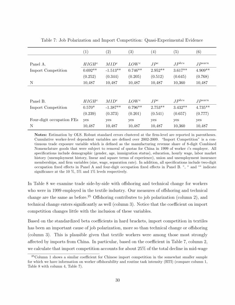
Table 7: Job Polarization and Import Competition: Quasi-Experimental Evidence
(1) (2) (3) (4) (5) (6)
Panel A. HIGHe MIDe LOW e JP e JP hrs JP earn
Import Competition 0.692** -1.513** 0.746** 2.952** 3.617** 4.909**
(0.252) (0.344) (0.205) (0.512) (0.645) (0.768)
N 10,487 10,487 10,487 10,487 10,360 10,487
Panel B. HIGHe MIDe LOW e JP e JP hrs JP earn
Import Competition 0.570* -1.387** 0.796** 2.753** 3.432** 4.735**
(0.239) (0.373) (0.201) (0.541) (0.657) (0.777)
Four-digit occupation FEs yes yes yes yes yes yes
N 10,487 10,487 10,487 10,487 10,360 10,487
Notes: Estimation by OLS. Robust standard errors clustered at the firm-level are reported in parentheses.Cumulative worker-level dependent variables are defined over 2002-2009. “Import Competition” is a con-tinuous trade exposure variable which is defined as the manufacturing revenue share of 8-digit CombinedNomenclature goods that were subject to removal of quotas for China in 1999 of worker i’s employer. Allspecifications include demographic (gender, age, immigration status), education, hourly wage, labor markethistory (unemployment history, linear and square terms of experience), union and unemployment insurancememberships, and firm variables (size, wage, separation rate). In addition, all specifications include two-digitoccupation fixed effects in Panel A and four-digit occupation fixed effects in Panel B. ◦, ∗ and ∗∗ indicatesignificance at the 10 %, 5% and 1% levels respectively.
In Table 8 we examine trade side-by-side with offshoring and technical change for workers
who were in 1999 employed in the textile industry. Our measures of offshoring and technical
change are the same as before.25 Offshoring contributes to job polarization (column 2), and
technical change enters significantly as well (column 3). Notice that the coefficient on import
competition changes little with the inclusion of these variables.
Based on the standardized beta coefficients in hard brackets, import competition in textiles
has been an important cause of job polarization, more so than technical change or offshoring
(column 3). This is plausible given that textile workers were among those most strongly
affected by imports from China. In particular, based on the coefficient in Table 7, column 2,
we calculate that import competition accounts for about 25% of the total decline in mid-wage
25Column 1 shows a similar coefficient for Chinese import competition in the somewhat smaller samplefor which we have information on worker offshorability and routine task intensity (RTI) (compare column 1,Table 8 with column 4, Table 7).
30

employment, compared to 17% in the economy at large.26
Table 8: Alternative Explanations to Import Competition: Quasi-Experimental Evidence
JP e JP e JP e
(1) (2) (3)
Import Competition 3.075** 3.033** 2.999**
(0.516) (0.514) (0.517)
[0.088] [0.087] [0.086]
Offshoring 0.160◦ 0.145
(0.087) (0.088)
[0.041] [0.037]
Routine Task Intensity 0.312*
(0.155)
[0.055]
Notes: N=9,127 in all columns. Estimation by two stage least squares. Robust standard errors clus-tered at the firm-level are reported in parentheses. Cumulative worker-level dependent variables aredefined over 2002-2009. “Import Competition” is a continuous trade exposure variable which is de-fined as the manufacturing revenue share of 8-digit Combined Nomenclature goods that were subjectto removal of quotas for China in 1999 of worker i’s employer. All regressions include demographic(gender, age, immigration status), education, hourly wage, labor market history (unemploymenthistory, linear and square terms of experience), union and unemployment insurance memberships,and firm variables (size, wage, separation rate). In all specifications workers’ initial occupations arecontrolled for using high-, mid-, and low-wage occupation indicators and occupation’s propensity tointeract with computers (varies at the four-digit occupation). ◦, ∗ and ∗∗ indicate significance at the10 %, 5% and 1% levels respectively.
We now address why import competition and technical change have distinct effects on job
polarization.
4.2 Import competition versus technical change: task-level evi-
dence
This section employs information on tasks from the U.S. Department of Labor’s O*NET
database at the level of individual workers in Denmark to distinguish the effect of trade
26We have also examined the question of within-versus-between sector employment effects in the case ofthis quasi-natural experiment, finding strong evidence that employment increases in the high- and low-wageoccupations are primarily in the service sector (see Table B-6 in the Online Appendix).
31

from that of technology.27 We interact the importance of a particular task in the worker’s
occupation with the degree to which this worker is exposed to rising import competition from
China. Our specification is the same as in Table 7, Panel A except that instead of two-digit
occupational fixed effects we include a measure of the importance of a particular task in
the worker’s four-digit occupation together with the interaction of this variable with import
exposure. All regressions include the full set of worker and firm variables from above.28
We span the task space by focusing on two dimensions, namely whether a task is routine or
non-routine (routine-ness dimension) and whether a task is manual or cognitive (manual di-
mension). We employ O*NET questions to map occupations with these tasks as employed in
the literature (Autor, Levy, Murnane 2003, Autor 2013, Firpo, Fortin, Lemieux 2011). Panel
A of Table 9 summarizes the results for four tasks: “Spend time making repetitive motions”,
“Pace Determined by Speed of Equipment”, “Manual Dexterity”, and “Finger Dexterity”.
These tasks are examples of routine manual tasks. Tasks in Panel B are non-routine manual
tasks, followed by routine cognitive tasks (Panel C), while non-routine cognitive tasks are
listed last (Panel D).
For each of the task indicators, Table 9 notes results for two different specifications, one
in which the dependent variable is mid-wage employment over 2002-2009 (MIDe), and
the other is HIGHe + LOW e −MIDe. Of key interest is the trade exposure-task content
interaction variable, whose sign and significance is shown in Table 9. Complete results for
these specifications are reported in the Online Appendix.
To begin with, the negative sign for the O*NET indicator “Spend time making repetitive
motions” in the MIDe regression indicates that exposed workers employed in occupations in
which repetitive motions are important experience larger declines in mid-wage employment
than the average exposed worker. The positive sign in the second column says that workers
in these occupations also have a higher likelihood of an increase in high- and low-wage
employment due to import competition. The finding that workers performing routine manual
tasks are susceptible to trade-induced job polarization is robust to considering other routine
manual tasks (rows 2 to 4 in Panel A). Strikingly, we find the same coefficient pattern for non-
routine manual tasks, such as “Gross Body Coordination” (Panel B). This is an important
finding because it shows that trade-induced job polarization occurs in occupations in which
workers perform manual tasks, whether these are routine or non-routine tasks.
27O*NET stands for Occupational Information Network. See the Online Appendix for details.28We also include indicators for working in high-, mid-, or low-wage occupations in 1999.
32

We now consider cognitive tasks with a high routine component (Panel C). An example
of this is “Evaluating Information to Determine Compliance with Standards”. It requires
cognitive abilities to judge compliance with standards, however it is a task performed in a
particular way and hence subject to some routine. For workers engaged in these tasks, import
competition reduces mid-wage employment by significantly less than for other observationally
similar exposed worker. These workers also see relatively low increases in high- and low-
wage employment, to the point that these workers do not much contribute to trade-induced
job polarization (see Table B-9 in the Online Appendix). We find the same pattern with
an alternative routine cognitive tasks measure, the importance of repeating the same task
(Panel C, second row).
Table 9: Signs of interaction between import competition and task variable
Dep. Var. MIDe JP e
A. Trade and Routine Manual TasksSpend time making repetitive motions - +Pace Determined by Speed of Equipment - +Manual Dexterity - +Finger Dexterity - +B. Trade and Non-Routine Manual TasksMultilimb Coordination - +Gross Body Coordination - +Response orientation - +C. Trade and Routine Cognitive TasksEvaluating Information to Determine Compliance with Standards + -Importance of Repeating Same Tasks + -D. Trade and Non-Routine Cognitive TasksMathematical Reasoning + -Inductive Reasoning + -Developing Objectives and Strategies + -Making Decisions and Solving Problems + -
Notes: Bold indicates significance at the standard levels based on robust standard errors that areclustered at the firm-level. Full results are provided in the Online Appendix.
Finally, we show results for workers performing intensively non-routine cognitive tasks, such
as those involving mathematical reasoning (Panel D). Exposed workers that perform such
tasks experience lower mid-wage employment declines than the typical exposed worker.
These workers are also less likely than the typical exposed worker to experience an increase
in low-wage employment (in fact, they do not gain low-wage employment at all: see the
Online Appendix), and overall, exposed workers performing abstract cognitive tasks hardly
33

contribute to job polarization. Panels C and D show that workers performing cognitive tasks
experience less trade-induced polarization, a result that is independent of whether the task
is routine or not.
Thus while technical change’s impact on job polarization depends on the routine-ness of
a task, the effect of import competition hinges on whether a task is cognitive or manual
in nature. In many countries computerized machines and robots have increasingly taken
over the performance of routine tasks. The fact that to date machines do not perform
certain non-routine tasks that well determines the extent to which domestic manufactures
are still produced by workers. Import competition, however, pits workers in Denmark against
workers in China. From this perspective it is not surprising that technical change and import
competition complement each other in explaining job polarization.
5 Normative implications of trade-induced job polar-
ization
While the previous analysis has focused on trade’s role in generating the U-shaped pattern
of job polarization, in this section we turn to a number of related normative issues. First, we
distinguish workers’ upward from downward movements, which have different welfare effects.
The impact of trade on hourly wages is also discussed. Second, this section quantifies the
contribution of import competition to recent changes in inequality. Third, we speak to the
educational policy debate by examining the performance of workers with different forms of
education. The analysis is based on the economy-wide sample of Section 3 and the same
instrumental variables approach employed before.
5.1 Upward versus downward movements and wages
We begin with the effect of rising import competition on employment and wages (Table 10,
Panels A and B, respectively). The analysis focuses on the n = 458,605 workers that were
employed in mid-wage occupations in the year 1999. Among these, those workers with high-
wage employment during the years 2000-2009 can be thought of moving up whereas those
with low-wage employment are the downward movers. Columns 1 and 3, respectively, show
the effect of rising import competition on these employment transitions.
34
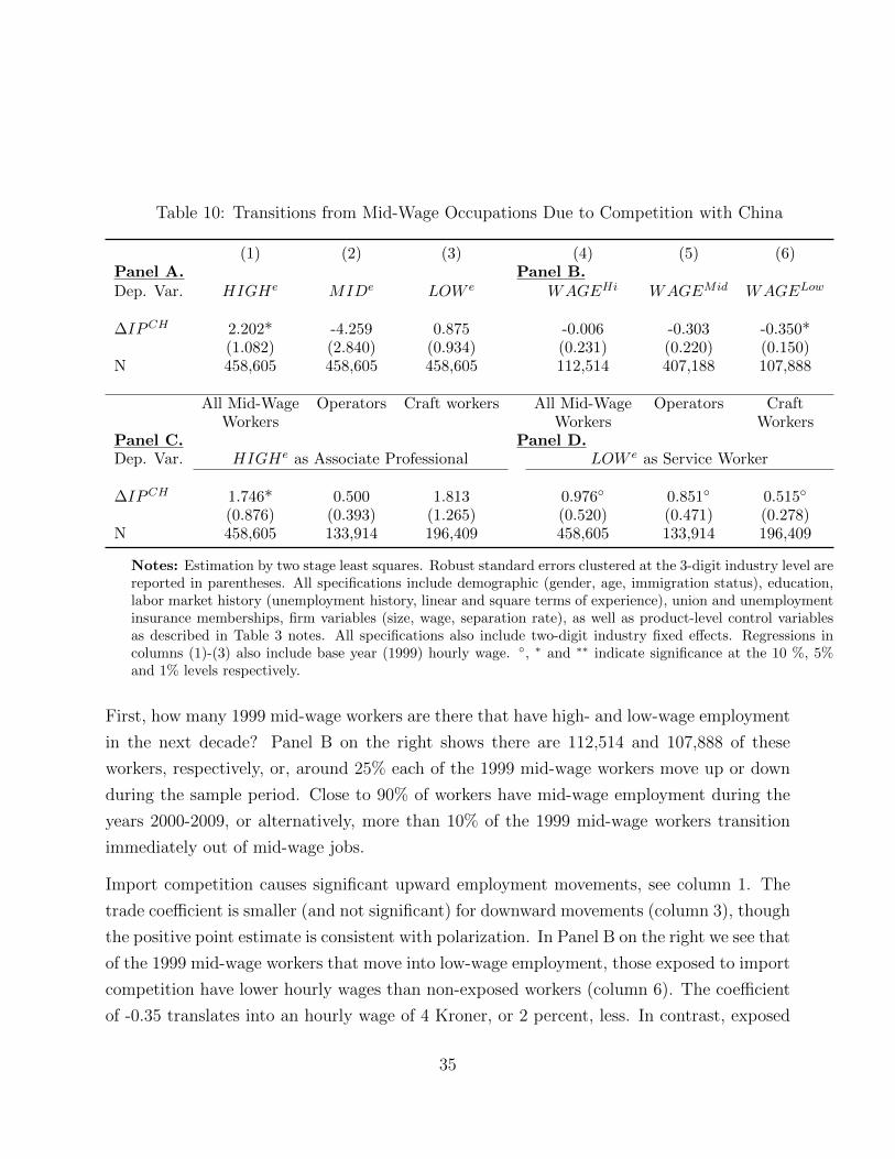
Table 10: Transitions from Mid-Wage Occupations Due to Competition with China
(1) (2) (3) (4) (5) (6)Panel A. Panel B.Dep. Var. HIGHe MIDe LOW e WAGEHi WAGEMid WAGELow
∆IPCH 2.202* -4.259 0.875 -0.006 -0.303 -0.350*(1.082) (2.840) (0.934) (0.231) (0.220) (0.150)
N 458,605 458,605 458,605 112,514 407,188 107,888
All Mid-Wage Operators Craft workers All Mid-Wage Operators CraftWorkers Workers Workers
Panel C. Panel D.Dep. Var. HIGHe as Associate Professional LOW e as Service Worker
∆IPCH 1.746* 0.500 1.813 0.976◦ 0.851◦ 0.515◦
(0.876) (0.393) (1.265) (0.520) (0.471) (0.278)N 458,605 133,914 196,409 458,605 133,914 196,409
Notes: Estimation by two stage least squares. Robust standard errors clustered at the 3-digit industry level arereported in parentheses. All specifications include demographic (gender, age, immigration status), education,labor market history (unemployment history, linear and square terms of experience), union and unemploymentinsurance memberships, firm variables (size, wage, separation rate), as well as product-level control variablesas described in Table 3 notes. All specifications also include two-digit industry fixed effects. Regressions incolumns (1)-(3) also include base year (1999) hourly wage. ◦, ∗ and ∗∗ indicate significance at the 10 %, 5%and 1% levels respectively.
First, how many 1999 mid-wage workers are there that have high- and low-wage employment
in the next decade? Panel B on the right shows there are 112,514 and 107,888 of these
workers, respectively, or, around 25% each of the 1999 mid-wage workers move up or down
during the sample period. Close to 90% of workers have mid-wage employment during the
years 2000-2009, or alternatively, more than 10% of the 1999 mid-wage workers transition
immediately out of mid-wage jobs.
Import competition causes significant upward employment movements, see column 1. The
trade coefficient is smaller (and not significant) for downward movements (column 3), though
the positive point estimate is consistent with polarization. In Panel B on the right we see that
of the 1999 mid-wage workers that move into low-wage employment, those exposed to import
competition have lower hourly wages than non-exposed workers (column 6). The coefficient
of -0.35 translates into an hourly wage of 4 Kroner, or 2 percent, less. In contrast, exposed
35

and non-exposed mid-wage workers moving into high-wage employment have virtually the
same hourly wages (column 4).
Thus, import competition has a more powerful upward employment effect than on downward
employment transitions. On net this can be seen as a positive effect. This quantity effect is
to some extent offset by the wage outcomes, because workers that are moving from mid- into
low-wage jobs due to import competition make relatively low hourly wages. These results are
confirmed when the definition of upward movements is extended to include transitions from
1999 low-wage workers to high-wage employment, and analogously, downward movements
include 1999 high-wage workers moving into low-wage employment. The upward quantity
impact of trade exposure is relatively strong, while at the same time wages of exposed workers
in low-wage occupations are relatively low as well (not shown).
Trade-induced upward movements for particular subsets of occupations are presented in
the lower part of Table 10. The first is transitions from any mid-wage occupations to as-
sociate professionals, a high-wage occupation (ISCO class 3; column 1). Next we present
the impact of import competition with China on the transition of plant and machine op-
erators (ISCO 8) and crafts workers (ISCO 7) to associate professionals (column 2 and 3).
Among the mid-wage workers, there are about 134,000 operators and 196,000 crafts work-
ers. Trade exposure significantly increases transitions into associate professional occupations
for all mid-wage workers (column 1). Comparing operators with crafts workers, though the
instrumental-variables estimates are not significant, we see that the relatively high point esti-
mate is evidence that craft workers are more likely to move upward into associate professional
occupations than operators (columns 2 and 3).
For trade-induced downward transitions we focus on the low-wage occupation of service and
shop workers (ISCO 5; see Panel D). The coefficient of just below one in column 4 means
that import exposure increases employment in these occupations by about 0.6 months on
average for the set of all 1999 mid-wage workers. This is quite close to the impact of trade
on operators, whereas craft workers transition to low-wage service occupations to a lesser
extent than the average worker in mid-wage occupation in 1999 (columns 5 and 6). In sum,
the typical craft worker can expect to do better in terms of trade-induced job polarization
than the typical operator: craft workers are both more likely to move up and less likely to
move down compared to machine operators. Overall, this analysis has shown that the result
of job polarization due to rising import competition holds up quite well even for transitions
between some of the most important individual occupations.
36
5.2 Import competition and inequality
While incomes in Denmark are traditionally distributed relatively equally, in recent years
inequality in Denmark has risen (Bjørnskov, Neamtu, and Westergard-Nielsen 2012). We
are interested in the implications of our analysis for inequality in Denmark as captured by
earnings of workers in different parts of the wage distribution. A simple measure of inequality
is the earnings share of workers in the tails, that is, the share of low-wage plus high-wage
earnings. More weight in the tails means higher inequality.
Employing the average 1999 wages paid in high-, mid-, and low-wage positions in Denmark,
the sum of high- and low-wage employment accounts for 48% of total sample earnings in
the year 1999. In contrast, the share of high- plus low-wage earnings has risen to 59.5%
by the year 2009, an increase in earnings inequality of 11.5 percentage points. Based on
the employment changes caused by rising import competition estimated in Table 4 and the
90/10 exposure difference, trade accounts for about 16% of the increase in earnings inequality.
Adjusting wages as they actually changed between 1999 and 2009 instead of holding wages
constant at the 1999 level increases the contribution of trade only slightly. We conclude that
rising import competition accounts for about 16% of the rise in inequality in Denmark, with
most of the effect due to quantity, not price (wage) changes.
5.3 Job polarization and education
This section considers education as a determinant of trade-induced job polarization. In
the first part we examine the impact of trade exposure on workers employment trajectories
depending on three levels of education (high school, vocational education, and college educa-
tion). Second, we contrast the performance of workers who have different forms of vocational
education.
We begin by including two additional interaction variables between exposure to trade and
education, ∆IPCH*College and ∆IPCH*HighSchool. As a consequence, the linear Chinese
import competition variable captures the impact of trade exposure on vocationally trained
workers (vocational training is the omitted category). Employment results are shown on the
left and wage results on the right side of Table 11.29
29All specifications include indicator variables for the three education levels, two-digit industry and occu-pation fixed effects, as well as the other covariates of our baseline specification (Table 3, column 5).
37
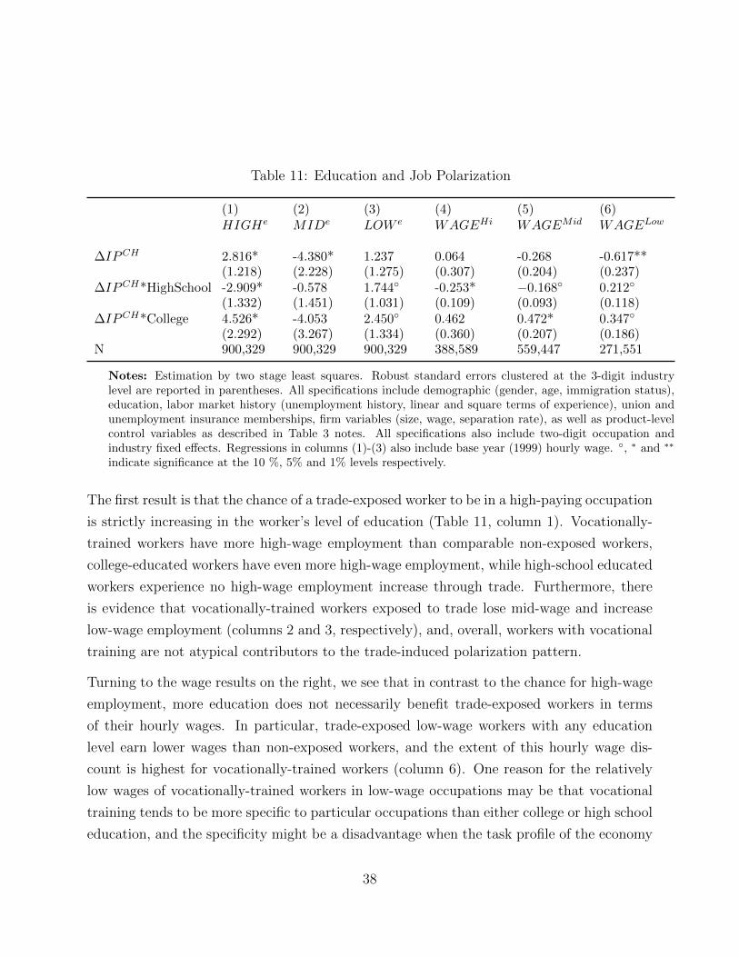
Table 11: Education and Job Polarization
(1) (2) (3) (4) (5) (6)HIGHe MIDe LOW e WAGEHi WAGEMid WAGELow
∆IPCH 2.816* -4.380* 1.237 0.064 -0.268 -0.617**(1.218) (2.228) (1.275) (0.307) (0.204) (0.237)
∆IPCH*HighSchool -2.909* -0.578 1.744◦ -0.253* −0.168◦ 0.212◦
(1.332) (1.451) (1.031) (0.109) (0.093) (0.118)∆IPCH*College 4.526* -4.053 2.450◦ 0.462 0.472* 0.347◦
(2.292) (3.267) (1.334) (0.360) (0.207) (0.186)N 900,329 900,329 900,329 388,589 559,447 271,551
Notes: Estimation by two stage least squares. Robust standard errors clustered at the 3-digit industrylevel are reported in parentheses. All specifications include demographic (gender, age, immigration status),education, labor market history (unemployment history, linear and square terms of experience), union andunemployment insurance memberships, firm variables (size, wage, separation rate), as well as product-levelcontrol variables as described in Table 3 notes. All specifications also include two-digit occupation andindustry fixed effects. Regressions in columns (1)-(3) also include base year (1999) hourly wage. ◦, ∗ and ∗∗
indicate significance at the 10 %, 5% and 1% levels respectively.
The first result is that the chance of a trade-exposed worker to be in a high-paying occupation
is strictly increasing in the worker’s level of education (Table 11, column 1). Vocationally-
trained workers have more high-wage employment than comparable non-exposed workers,
college-educated workers have even more high-wage employment, while high-school educated
workers experience no high-wage employment increase through trade. Furthermore, there
is evidence that vocationally-trained workers exposed to trade lose mid-wage and increase
low-wage employment (columns 2 and 3, respectively), and, overall, workers with vocational
training are not atypical contributors to the trade-induced polarization pattern.
Turning to the wage results on the right, we see that in contrast to the chance for high-wage
employment, more education does not necessarily benefit trade-exposed workers in terms
of their hourly wages. In particular, trade-exposed low-wage workers with any education
level earn lower wages than non-exposed workers, and the extent of this hourly wage dis-
count is highest for vocationally-trained workers (column 6). One reason for the relatively
low wages of vocationally-trained workers in low-wage occupations may be that vocational
training tends to be more specific to particular occupations than either college or high school
education, and the specificity might be a disadvantage when the task profile of the economy
38

undergoes rapid changes.
In general, vocationally trained, mid-skill, workers contribute to job polarization as we have
seen above (Table 11, first row, columns 1 to 3). Since it might be important to separate
workers holding different forms of vocational education, in the following we narrow the focus
to workers who are trained for manufacturing vocations, such as welders, toolmakers, or
industrial cabinet makers, versus workers trained for service vocations, such as orthopedic
technicians, office workers, or decorators. Within the group of workers trained for service
vocations we present separate results for the set of workers trained for information-technology
(IT) related vocations, e.g. IT assistants.30
In Table 12 we present results where we interact our exposure to import competition variable
with an indicator variable for particular forms of vocational training that worker i has com-
pleted: specific to the manufacturing sector (MVoc), service sector (SVoc), and information
technology (ITVoc) vocations, respectively in Panels A, B, and C.31 The impact of trade ex-
posure on mid-wage employment of vocationally trained workers with manufacturing focus
is equal to about -2.1, which is the sum of the two coefficients shown in Table 12 (Panel A,
column 2). This translates into a smaller mid-wage employment reduction than either the
average vocationally trained worker (-4.4, Table 11, column 2) or the typical worker that
is not vocationally trained with a manufacturing focus (-6.0, Table 12, column 2). Thus, a
formal education on manufacturing vocations shields a worker to some extent from mid-wage
employment reductions as these workers are highly skilled for manufacturing.
30This classification has been obtained by coding around 3,000 of the education titles available in Denmark;see the Online Appendix section 1.2 for details.
31All specifications include indicator variables for each of these education levels.
39
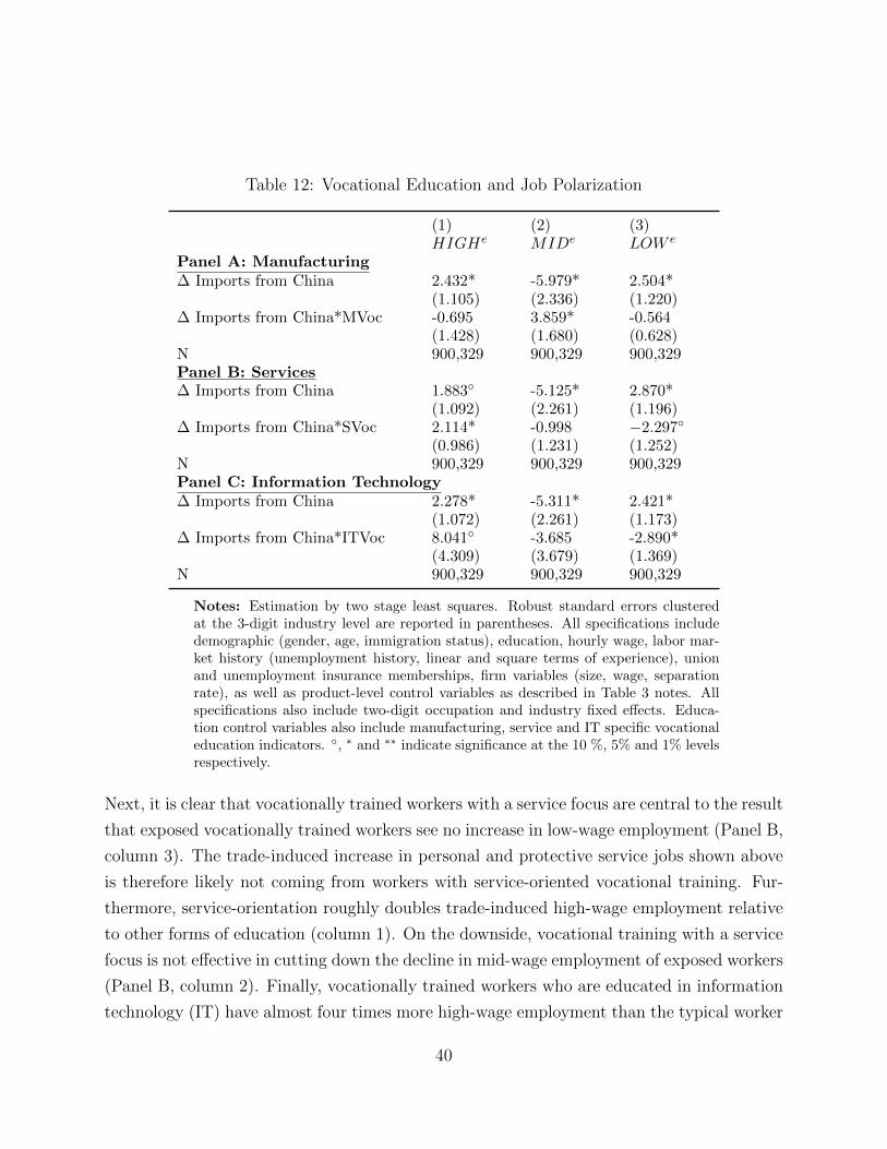
Table 12: Vocational Education and Job Polarization
(1) (2) (3)HIGHe MIDe LOW e
Panel A: Manufacturing∆ Imports from China 2.432* -5.979* 2.504*
(1.105) (2.336) (1.220)∆ Imports from China*MVoc -0.695 3.859* -0.564
(1.428) (1.680) (0.628)N 900,329 900,329 900,329Panel B: Services∆ Imports from China 1.883◦ -5.125* 2.870*
(1.092) (2.261) (1.196)∆ Imports from China*SVoc 2.114* -0.998 −2.297◦
(0.986) (1.231) (1.252)N 900,329 900,329 900,329Panel C: Information Technology∆ Imports from China 2.278* -5.311* 2.421*
(1.072) (2.261) (1.173)∆ Imports from China*ITVoc 8.041◦ -3.685 -2.890*
(4.309) (3.679) (1.369)N 900,329 900,329 900,329
Notes: Estimation by two stage least squares. Robust standard errors clusteredat the 3-digit industry level are reported in parentheses. All specifications includedemographic (gender, age, immigration status), education, hourly wage, labor mar-ket history (unemployment history, linear and square terms of experience), unionand unemployment insurance memberships, firm variables (size, wage, separationrate), as well as product-level control variables as described in Table 3 notes. Allspecifications also include two-digit occupation and industry fixed effects. Educa-tion control variables also include manufacturing, service and IT specific vocationaleducation indicators. ◦, ∗ and ∗∗ indicate significance at the 10 %, 5% and 1% levelsrespectively.
Next, it is clear that vocationally trained workers with a service focus are central to the result
that exposed vocationally trained workers see no increase in low-wage employment (Panel B,
column 3). The trade-induced increase in personal and protective service jobs shown above
is therefore likely not coming from workers with service-oriented vocational training. Fur-
thermore, service-orientation roughly doubles trade-induced high-wage employment relative
to other forms of education (column 1). On the downside, vocational training with a service
focus is not effective in cutting down the decline in mid-wage employment of exposed workers
(Panel B, column 2). Finally, vocationally trained workers who are educated in information
technology (IT) have almost four times more high-wage employment than the typical worker
40

with other education (Panel C, column 1). While we know that college education matters
for high-wage employment gains (Table 11, column 1), comparing column 1 of Panel A with
Panel C also indicates that mid-skilled workers trained for information technology (IT) vo-
cations have more than five times more high-wage employment than other observationally
similar mid-skilled workers with manufacturing focus.32 Furthermore, there is no evidence
that workers with IT education who are exposed to import competition move into low-wage
jobs (column 3).
The picture that emerges from these results is that a while manufacturing focus in vocational
training raises the chance that workers experience smaller mid-wage employment declines,
it does not prevent workers from shifting into low-wage employment. In contrast, service
orientation in vocational training by and large eliminates the chance that exposed workers
shift into low-wage jobs, and strongly increases the chance that a worker moves into high-
wage occupations. Outcomes are highly heterogeneous for workers with different forms
of vocational education. Overall, whatever temporary protection manufacturing orientation
gives in mid-wage occupations has to be compared with the relatively high long-run earnings
potential that appears to come only with certain service-oriented vocational training or
college education.
6 Conclusions
Employing matched worker-firm data for much of Denmark’s economy during the early 2000s
we have shown that competition with China can explain job polarization in high-income
countries. Individual transitions between sectors, observed through worker-level data, are
crucial for the U-shaped employment changes of job polarization. Overwhelmingly rising
import competition impacts manufacturing workers earning mid-level wages. Outcomes are
heterogeneous, with some workers moving up and others down in the wage distribution.
Low-wage employment increases are mainly in services, in contrast to trade–induced gains
in high-wage employment, which are split between manufacturing and the service sector.
The up- versus down movement hinges primarily on workers’ education. Short of college
education—which takes relatively long and is arguably not for everyone—, vocational train-
ing has promise if it is targeted to certain service occupations, especially those involving
32We arrive at the same conclusion when we conduct the analysis only among vocationally trained workers,see Table B-11 in the Online Appendix.
41

technical and computer skills.
Our first conclusion follows directly from finding that import competition is a quantitatively
important cause of job polarization. Consequently, the debate about job polarization as
a phenomenon, and what it implies for government policy, can from now on consider not
only technical change but also rising import competition. In particular, policy initiatives
towards trade reform need to consider the strong possibility that in high-income countries,
job polarization is a likely outcome. Conversely, some of the concerns about the impact of
information & communication technologies (ICTs) on worker outcomes can be put to rest
because the outcomes are actually due to import competition, not technical change.
A critic might question that any of this matters. Aren’t trade, offshoring, and technical
change all just different facets of globalization that are inextricably linked? There is no
doubt that offshoring is related to ICT innovations, or that not only abundant unskilled labor
but also industrial robots (and hence ICT) have contributed to the rising export capacity
in emerging countries.33 However this does not mean that one should give up analyzing
the unique drivers of each of the job polarization causes. In our worker-task analysis we
have shown that the influence of technical change and import competition can be clearly
delineated. We expect that future research can go much further along these lines.
Second, rising import competition does not only have the well-documented negative effects on
employment and (nominal) earnings of workers in high-income countries. Import competition
moves some workers into high-wage jobs, accounting for about 8% of the total increase
in high-wage employment in Denmark during the early 2000s. For these workers, import
competition provides the incentive to switch to a high-wage career path. Import competition,
in the words of Schumpeter, is a force of creative destruction. This important point has not
been emphasized in the recent trade and labor literature. It does not mean that this shift for
some workers to high-wage jobs is costless in the short run. However, we can now start to
think about how to make medium-term transitions to high-earning career paths more likely.
The debate about globalization gains in high-wage countries does not have to start and end
largely with the observation that globalization makes many goods cheaper in high-income
countries.
Our treatment of technical change and offshoring differs somewhat from the way we approach
the role of import competition. In particular, it is one thing to show that jobs with a high
33China is the largest buyer of industrial robots in the world since 2014, Financial Times (2014).
42
degree of offshorability contribute to job polarization, but it is another to show that offshoring
actually causes job polarization. Similarly, one might prefer an analysis of technical change
in terms of computers instead of the task characteristics of workers that are replaced by
computers. Given our emphasis on the role of import competition we adopt a conservative
approach and treat any association with offshoring and technical change as these factors
causing job polarization. While this arguably does not stack the analysis in favor of finding
a major role for import competition, it would be useful for future work to employ direct
measures and comparable identification strategies for all suspected causes of job polarization
and other labor market outcomes of globalization.
References
[1] Autor, David 2010. “The Polarization of Job Opportunities in the U.S. Labor Market:
Implications for Employment and Earnings”, Center for American Progress and The
Hamilton Project.
[2] Autor, David 2013. “The “task approach” to labor markets: an overview”, Journal
for Labour Market Research, 46(3): 185-199.
[3] Autor, David, and David Dorn 2013. “The Growth of Low-Skill Service Jobs and the
Polarization of the US Labor Market”, American Economic Review, 103(5): 1553-1597.
[4] Autor, David, David Dorn, and Gordon Hanson. 2013. “The China Syndrome:
Local Labor Market Effects of Import Competition in the United States”, American
Economic Review, 103(6): 2121-2168.
[5] Autor, David, David Dorn, and Gordon Hanson. 2015. “Untangling Trade and
Technology: Evidence from local Labor Markets”, Economic Journal, 125(584): 621-
646.
[6] Autor, David, David Dorn, Gordon Hanson and Jae Song. 2014. “Trade Adjust-
ment: Worker Level Evidence”, The Quarterly Journal of Economics, 129: 1799-1860.
[7] Autor, David, Lawrance F. Katz, and Melissa S. Kearney 2006. “The Polariza-
tion of the U.S. Labor Market”, American Economic Review: Papers and Proceedings,
96(2), 189-193.
[8] Autor, David, Lawrance F. Katz, and Melissa S. Kearney 2008. “Trends in U.S.
Wage Inequality: Revising the Revisionists”, The Review of Economics and Statistics,
90(2), 300-323.
43
[9] Autor, David, Levy, Frank, and Richard Murnane 2003. “The Skill-Content
of Recent Technological Change: An Empirical Investigation”, Quarterly Journal of
Economics, 118, 1279-1333.
[10] Bagger, Jesper, Bent Jesper Christensen, and Dale T. Mortensen 2014. “Wage
and labor productivity dispersion: The roles of total factor productivity, labor quality,
capital intensity, and rent sharing.”, Working paper.
[11] Becker, Sascha O. and Marc-Andreas Muendler 2015. “Trade and tasks: an
exploration over three decades in Germany”, Economic Policy, 30(84): 589-641.
[12] Bernard, Andrew B., Bradford J. Jensen and Peter K. Schott 2006. “Survival
of the best fit: Exposure to low-wage countries and the (uneven) growth of U.S. manu-
facturing plants”, Journal of International Economics, Elsevier, vol. 68(1), 219-237.
[13] Bjørnskov, Christian, Ioana Neamtu, and Niels Westergard-Nielsen 2012.
“Growing Inequality And Its Impacts In Denmark”, GINI Country Report for Denmark.
[14] Blinder, Alan, and Alan Krueger 2013. “Alternative Measures of Offshorability: A
Survey Approach”, Journal of Labor Economics, 31(2): S97-S128
[15] Bloom, Nicholas, Mirko Draca, and John Van Reenen 2016. “Trade induced
technical change? The impact of Chinese imports on innovation and information tech-
nology”, Review of Economic Studies, 83: 87-117
[16] Brambilla, Irene, Amit Khandelwal and Peter Schott 2010. “China’s Experience
Under the Multifiber Arrangement (MFA) and the Agreement on Textile and Clothing
(ATC)”, Robert Feenstra and Shang-Jin Wei (Eds), China’s Growing Role in World
Trade, NBER, Cambridge: MA.
[17] Brandt, Loren, Chang-Tai Hsieh, and Xiaodong Zhu 2008. “Growth and Struc-
tural Transformation in China.” In China’s Great Economic Transformation, edited by
Loren Brandt and Thomas G. Rawski, 683-728. Cambridge University Press.
[18] Bunzel, Henning 2008. “The LMDG Data Sets”, mimeo, Univeristy of Aarhus.
[19] Dix-Carneiro, Rafael 2014. “Trade Liberalization and Labor Market Dynamics”,
Econometrica, 82(3): 825-885.
[20] Dix-Carneiro, Rafael, and Brian Kovak 2015. “Trade Reform and Regional Dy-
namics: Evidence From 25 Years of Brazilian Matched Employer-Employee Data”, un-
published manuscript.
[21] Dustmann, Christian, Johannes Ludsteck, and Uta Schonberg 2009. “Revisit-
ing the German Wage Structure”, The Quarterly Journal of Economics, 124, 843-881.
44
[22] Ebenstein, Avraham, Ann Harrison, Margaret McMillan and Shannon
Phillips 2014. “Estimating the Impact of Trade and Offshoring on American Work-
ers using the Current Population Surveys”, The Review of Economics and Statistics,
96(3): 581-595.
[23] Eriksson, Tor and Niels Westergaard-Nielsen 2009. “Wage and Labor Mobility in
Denmark, 1980-2000”, appeared in The Structure of Wages: An International Compar-
ison, (Eds.) Edward P. Lazear and Kathryn L. Shaw, Chicago: University of Chicago
Press and National Bureau of Economic Research.
[24] Financial Times 2014. “China becomes largest buyer of industrial robots”, June 1
2014. http://www.ft.com/intl/cms/s/0/a5cca8c0-e70c-11e3-aa93-00144feabdc0.html
[25] Firpo, Sergio, Nicole Fortin, and Thomas Lemieux 2011. “Occupational Tasks
and Changes in the Wage Structure”, IZA Discussion Paper 5542, Institute for the
Study of Labor (IZA).
[26] Foged, Mette and Giovanni Peri 2016. “Immigrants’ Effect on Native Workers: New
Analysis on Longitudinal Data”, American Economic Journal: Applied Economics, 8(2):
1-34.
[27] Goldberg, Pinelopi and Nina Pavcnik 2007. “Distributional Effects of Globaliza-
tion in Developing Countries, Journal of Economic Literature, 45(1), pp. 39-82.
[28] Goos, Maarten, and Alan Manning 2007. “Lousy and Lovely Jobs: The Rising
Polarization of Work in Britain”, The Review of Economics and Statistics, 89(1), 118-
133.
[29] Goos, Maarten, Alan Manning, and Anna Salomons 2009. “Job Polarization in
Europe”, American Economic Review: Papers and Proceedings, 99(2), 58-63.
[30] Goos, Maarten, Alan Manning, and Anna Salomons 2014. “Explaining Job Po-
larization: Routine-Biased Technological Change and Offshoring”, American Economic
Review, 104(8), 2509-2526.
[31] Graetz, Georg and Guy Michaels 2015 “Robots at Work”, Center for Economic
Performance Discussion Paper No. 1335.
[32] Groes, Fane, Philipp Kircher, and Iorii Manovskii 2015. “The U-Shapes of Oc-
cupational Mobility”, Review of Economic Studies, 82(2): 659-692.
[33] Hakobyan, Shushanik and John McLaren 2016. “Looking for Local Labor-Market
Effects of NAFTA”, The Review of Economics and Statistics, forthcoming.
45
[34] Harrigan, James, Ariell Reshef, and Farid Toubal 2015. “The March of the
Techies: Technology, Trade, and Job Polarization in France, 1994-2007”, presented at
NBER ITI Winter Meeting 2015.
[35] Harrison Ann, John McLaren, Margaret McMillan 2011. “Recent Perspectives
on Trade and Inequality”, Annual Review of Economics, Vol 3, pp 261-289.
[36] Haskel, Jonathan E., Sonia C. Pereira, and Matthew J. Slaughter 2007. “Does
Inward Foreign Direct Investment Boost The Productivity Of Domestic Firms?”, The
Review of Economics and Statistics, August 2007, 89(3): 482-496.
[37] Holzer, Harry 2015. “Job Market Polarization and U.S. Worker Skills: A Tale of Two
Middles”, Economic Studies, The Brookings Institution.
[38] Hummels, David, Rasmus Jorgensen, Jacob Munch, and Chong Xiang 2014.
“The Wage Effects of Offshoring: Evidence From Danish Matched Worker-Firm Data”,
American Economic Review, 104(6): 1597-1629.
[39] Kovak, Brian 2013. “Regional Effects of Trade Reform: What Is the Correct Measure
of Liberalization?”, American Economic Review, 103(5):1960-1976.
[40] Khandelwal, Amit, Peter Schott and Shang-Jin Wei 2013. “Trade Liberalization
and Embedded Institutional Reform: Evidence from Chinese Exporters”, American
Economic Review, Vol. 103(6): 2169-2195.
[41] Koopman, Robert, Zhi Wang, and Shang-Jin Wei 2014. “Tracing Value-Added
and Double Counting in Gross Exports”, American Economic Review, 104(2): 459-94.
[42] Leonhardt, D. 2015. “College for the Masses”, New Yorkt Times, Apr 24, 2015.
[43] Michaels, Guy, Ashwini Natraj and John Van Reenen 2014. “Has ICT Polarized
Skill Demand? Evidence From Eleven Countries Over Twenty-Five Years”, The Review
of Economics and Statistics, 96(1), 60-77.
[44] Moretti, Enrico 2012. The New Geography of Jobs. New York: Houghton Mifflin
Harcourt.
[45] Pierce, Justin R. and Peter K. Schott. 2014. “The Surprisingly Swift Decline of
U.S. Manufacturing Employment”, American Economic Review, forthcoming.
[46] Quinton, Sophie 2015. “Could Vocational Education be the Answer to Failing High
Schools?”, The Atlantic, Apr 15, 2015.
[47] Schwartz, Nelson 2013. “Where Factory Apprenticeship Is Latest Model From Ger-
many”, New York Times, Nov 30, 2013.
46

[48] Spitz-Oener, Alexandra 2006. “Technical Change, Job Tasks and Rising Educational
Demand: Looking Outside the Wage Structure”, Journal of Labor Economics, 24, 235-
270.
[49] The Economist 2010. “Too narrow, too soon? Americas misplaced disdain for voca-
tional education”, June 17, 2010.
[50] Timmermans, Bram 2010. “The Danish Integrated Database for Labor Market Re-
search: Towards Demystification for the English Speaking Audience”, DRUID Working
Papers 10-16.
[51] Utar, Hale 2014. “When the Floodgates Open: ”Northern” Firms’ Response to Re-
moval of Trade Quotas on Chinese Goods”, American Economic Journal: Applied Eco-
nomics, 6(4): 226-250.
[52] Utar, Hale 2015. “Workers beneath the Floodgates: Impact of Low-Wage Import
Competition and Workers’ Adjustment”, Bielefeld Working Papers in Economics and
Management, No.12.
[53] Utar, Hale, and Luis Torres Ruiz. 2013. “International Competition and Industrial
Evolution: Evidence from the Impact of Chinese Competition on Mexican Maquilado-
ras”, Journal of Development Economics, 105: 267-287.
[54] World Bank 2016. World Development Indicators databese, merchandise exports.
[55] Wyman, Nicholas 2015. “Why we desparately need to bring back vocational training
in schools”, Forbes, Sept 1, 2015.
Descriptive Statistics
47

Table A-1: Ranking of Major Occupations in Denmark
Occupation Median Log Mean Log Employment CorrespondingHourly Wage Hourly Wage Share Major1999 2009 1999 2009 1999 2009 ISCO
High-WageLegislators, Senior Officials, and Managers 5.488 5.550 5.538 5.604 0.038 0.039 1Professionals 5.297 5.362 5.349 5.412 0.145 0.168 2Technicians and Associate Professionals 5.116 5.177 5.160 5.211 0.184 0.239 3Mid-WageCraft and Related Trade Workers 5.053 5.098 5.002 5.034 0.128 0.091 7Plant and Machine Operators and Assemblers 5.012 5.088 5.095 5.024 0.089 0.062 8Clerks 4.949 5.013 4.945 5.023 0.134 0.103 4Low-WageElementary Occupations in Sales, Services, 4.919 4.962 4.928 4.956 0.117 0.104 9Mining, Construction, Manufacturing, (except 92)and TransportService Workers and Shop Sales Workers 4.849 4.938 4.851 4.927 0.165 0.193 5
Notes: Values are expressed in 2000 Danish Kroner. All hourly wages are calculated among workers with full-time jobsemployed continuously with at least one year tenure. Employment shares are calculated using the number of employeesand excluding army and agriculture/fishery occupations.
48
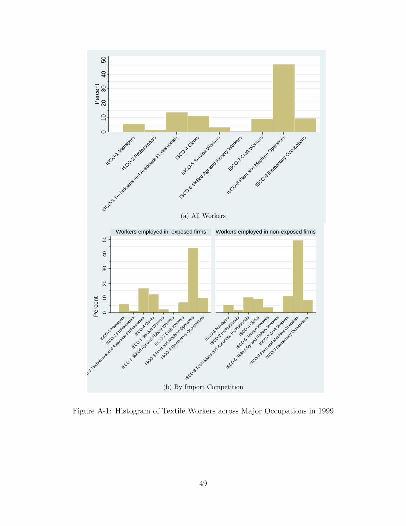
010
2030
4050
Per
cent
ISCO-1
Man
ager
s
ISCO-2
Pro
fess
ionals
ISCO-3
Tec
hnici
ans a
nd A
ssoc
iate
Profe
ssion
als
ISCO-4
Cler
ks
ISCO-5
Ser
vice
Wor
kers
ISCO-6
Skil
led A
gr a
nd F
isher
y Wor
kers
ISCO-7
Cra
ft W
orke
rs
ISCO-8
Plan
t and
Mac
hine
Opera
tors
ISCO-9
Elem
enta
ry O
ccup
ation
s
(a) All Workers
010
2030
4050
ISCO-1
Man
ager
s
ISCO-2
Pro
fess
ionals
ISCO-3
Tec
hnici
ans a
nd A
ssoc
iate
Profe
ssion
als
ISCO-4
Cler
ks
ISCO-5
Ser
vice
Wor
kers
ISCO-6
Skil
led A
gr a
nd F
isher
y Wor
kers
ISCO-7
Cra
ft W
orke
rs
ISCO-8
Plan
t and
Mac
hine
Opera
tors
ISCO-9
Elem
enta
ry O
ccup
ation
s
ISCO-1
Man
ager
s
ISCO-2
Pro
fess
ionals
ISCO-3
Tec
hnici
ans a
nd A
ssoc
iate
Profe
ssion
als
ISCO-4
Cler
ks
ISCO-5
Ser
vice
Wor
kers
ISCO-6
Skil
led A
gr a
nd F
isher
y Wor
kers
ISCO-7
Cra
ft W
orke
rs
ISCO-8
Plan
t and
Mac
hine
Opera
tors
ISCO-9
Elem
enta
ry O
ccup
ation
s
Workers employed in exposed firms Workers employed in non-exposed firms
Per
cent
(b) By Import Competition
Figure A-1: Histogram of Textile Workers across Major Occupations in 1999
49

Table A-2: Textile Workers’ Characteristics in 1999 by Selective Occupations and Import Exposure
Mean Standard
Deviation
N
Weaving and Knitting Machine Operators employed in non-exposed firmsAge 40.566 10.479 304Female 0.247 0.432 304Immigrant 0.089 0.285 304College Educated 0.043 0.203 304Years of Experience in the Labor Market 15.740 5.439 304Unemployment History 1.012 1.509 304Weaving and Knitting Machine Operators employed in exposed firmsAge 41.966 9.459 205Female 0.288 0.454 205Immigrant 0.112 0.316 205College Educated 0.049 0.216 205Years of Experience in the Labor Market 16.493 4.813 205Unemployment History 1.122 1.558 205Sewing Machine Operators employed in non-exposed firmsAge 42.849 9.368 537Female 0.946 0.226 537Immigrant 0.143 0.351 537College Educated 0.020 0.142 537Years of Experience in the Labor Market 15.294 5.579 537Unemployment History 2.574 2.512 537Sewing Machine Operators employed in exposed firmsAge 43.257 10.026 915Female 0.957 0.202 915Immigrant 0.072 0.259 915College Educated 0.026 0.160 915Years of Experience in the Labor Market 16.216 5.255 915Unemployment History Index 1.429 1.695 915Post-Processing Textile Machine Operators employed in non-exposed firmsAge 40.478 9.894 502Female 0.329 0.470 502Immigrant 0.084 0.277 502College Educated 0.064 0.245 502Years of Experience in the Labor Market 14.964 5.535 502Unemployment History 1.375 1.737 502Post-Processing Textile Machine Operators employed in exposed firmsAge 39.030 9.667 133Female 0.323 0.470 133Immigrant 0.045 0.208 133College Educated 0.030 0.171 133Years of Experience in the Labor Market 15.609 5.145 133Unemployment History 1.465 2.003 133Cutting, Rope Making, Netting, Leather Textile Machine Operators in non-exposed firmsAge 39.888 9.311 251Female 0.199 0.400 251Immigrant 0.008 0.089 251College Educated 0.020 0.140 251Years of Experience in the Labor Market 16.275 4.791 251Unemployment History 1.713 2.117 251Cutting, Rope Making, Netting, Leather Textile Machine Operators in exposed firmsAge 40.466 10.201 221Female 0.674 0.470 221Immigrant 0.081 0.274 221College Educated 0.032 0.176 221Years of Experience in the Labor Market 15.330 5.396 221Unemployment History 1.619 2.069 221
50

Supplementary Appendix for:
“International Trade and Job Polarization:
Evidence at the Worker Level”
Wolfgang Keller
Hale Utar
May 30, 2016
1

1 Data
The main database employed in this study is the Integrated Database for Labour
Market Research (abbreviated IDA), which is compiled from person (IDA-personer),
establishment (IDA-arbejdssteder), and job files (IDA-ansættelser) by Statistics Den-
mark. We supplement this database with the domestic production dataset (abbreviated
VARES), a dataset on business statistics (abbreviated FIRE), and the dataset on cus-
toms transactions (abbreviation UHDI). These datasets are accessed through the servers
sponsored by the Labor Market Development and Growth (LDMG) project. Informa-
tion on import quotas for the European Union textile and clothing sector comes from
the Systeme Integre de Gestion de Licenses (abbreviated SIGL) database, which is
available online at http://trade.ec.europa.eu/sigl/index.html. Information on the task
content of occupations employed in this paper comes from the U.S. Bureau of La-
bor Statistics O*NET database, version 14. Below we provide a brief description of
this data. More detailed information regarding the Danish data can be accessed at
http://www.dst.dk/da/Statistik/dokumentation/Times .
Integrated Database for Labor Market Research (IDA)
The IDA Database is the main source of information on workers. It provides a snapshot
of the labor market for each year at the end of November. It contains demographic and
education information on every resident in Denmark between the age of 15 and 74 with
a unique personal identification number. Compiled from separate establishment and job
files, it provides the labor market status of each individual, as well as the annual salary
and hourly wage, occupational position, and industry code of their primary employment.
We describe the information on industry, education, and occupation in greater detail
below.
Production Database (VARES)
The database is part of the industrial commodity production statistics (abbreviated
2
PRODCOM) collected by Statistics Denmark. Production is reported following the
Combined Nomenclature (CN) classification at the eight-digit level for all firms with ten
or more employees. We employ the VARES database to identify firms that manufacture
domestically in Denmark products subject to rising competition due to the removal of
import quotas (the Multi-fiber Arrangement) on Chinese goods after 2001. While some
manufacturing firms have less than ten employees, such firms typically outsource their
production, and consequently we can identify virtually all firms that domestically pro-
duce quota products using VARES. The reporting unit is the “Kind of Activity Unit”
(KAU), which is the sum of a company’s workplaces in the same main industry. Report-
ing units provide as well their company identification code (abbreviated CVR), allowing
us to match the eight-digit production information with other firm-level information.
Business and accounting statistics (FIRE)
This dataset by Statistics Denmark compiles business and accounting data, as well as
tax reports, value-added tax (VAT) reports, and information from incorporated compa-
nies. It is employed in this paper to create the pre-trend variable in the firm’s product
category as well as other measures at the six-digit level. The information covers virtu-
ally all firms for most sectors (including manufacturing, construction, retail, mining, as
well as hospitality, transportation, telecommunication, real estate, rental, information
technology, R&D and other business services).1
1Firms must satisfy certain minimum sizes: at least 0.5 full-time equivalent employment, as wellas certain minimum sales, between 150,000 and 200,000 Danish Kroner in manufacturing and 500,000Danish Kroner in wholesale trade. 1 Danish Kroner is about 0.15 $ US in 2016.
3
International trade data (UHDI)
The data comes from Denmark’s customs records together with monthly reports to
Statistics Denmark from about 8,000 firms in Denmark in which their trade with other
countries of the European Union (EU) is reported. This is supplemented with infor-
mation on EU trade from VAT returns, which are mandatory for virtually all firms in
Denmark. The information of each record gives shipment date, value, and weight, and if
applicable the shipment’s quantity. It also provides information on the 8-digit product
classification according to the Combined Nomenclature (CN) system, as well as a unique
firm identifier. Statistics Denmark aggregates this data into annual information for each
triplet of product-firm-country. The information is employed to identify firms (and their
workers) that are subject to rising import competition from China.
Textile quota data (SIGL)
The Systeme Integre de Gestion de Licenses (SIGL) database of the World Trade Or-
ganization (WTO) provides categories of textile and clothing products that are subject
to trade quotas in the European Union for a particular year. We employ this data to
identify firms in Denmark that will be affected by the quota removals on Chinese exports
following that country’s entry into the WTO. The quota categories are administrative
descriptions of quota products that do not follow standard statistical product classifica-
tions. The quotas have a varying degree of coverage; for example, the quota category
“Gloves, mittens and mitts, knitted or crocheted” covers nine products at the 8-digit
CN level, while the category “Woven fabrics of synthetic filament yarn obtained from
strip or the like of polyethylene or polypropylene, less than 3 m wide” corresponds to a
single 8-digit CN product. Quota categories include both textile and clothing products.
A given category does not necessarily cover a technologically or materially homogeneous
group of products, nor does it have to be comprehensive. For example, ramie bed-
spreads are covered by the quota restriction for China while cotton bedspreads are not,
and “Brasseries of all types of textile material” is covered, in contrast to “Corselettes of
4
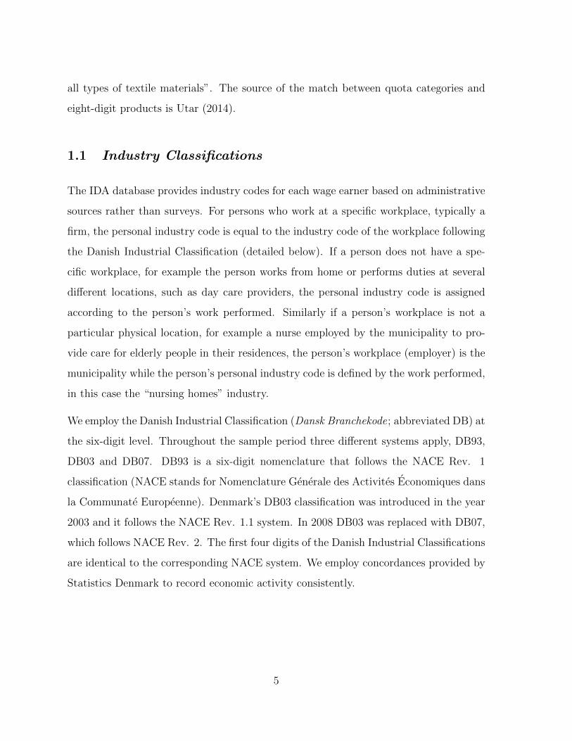
all types of textile materials”. The source of the match between quota categories and
eight-digit products is Utar (2014).
1.1 Industry Classifications
The IDA database provides industry codes for each wage earner based on administrative
sources rather than surveys. For persons who work at a specific workplace, typically a
firm, the personal industry code is equal to the industry code of the workplace following
the Danish Industrial Classification (detailed below). If a person does not have a spe-
cific workplace, for example the person works from home or performs duties at several
different locations, such as day care providers, the personal industry code is assigned
according to the person’s work performed. Similarly if a person’s workplace is not a
particular physical location, for example a nurse employed by the municipality to pro-
vide care for elderly people in their residences, the person’s workplace (employer) is the
municipality while the person’s personal industry code is defined by the work performed,
in this case the “nursing homes” industry.
We employ the Danish Industrial Classification (Dansk Branchekode; abbreviated DB) at
the six-digit level. Throughout the sample period three different systems apply, DB93,
DB03 and DB07. DB93 is a six-digit nomenclature that follows the NACE Rev. 1
classification (NACE stands for Nomenclature Generale des Activites Economiques dans
la Communate Europeenne). Denmark’s DB03 classification was introduced in the year
2003 and it follows the NACE Rev. 1.1 system. In 2008 DB03 was replaced with DB07,
which follows NACE Rev. 2. The first four digits of the Danish Industrial Classifications
are identical to the corresponding NACE system. We employ concordances provided by
Statistics Denmark to record economic activity consistently.
5

1.2 Education
The IDA-personer files specify for each individual the level of the highest completed
education or professional training (Erhvervskompetancegivende uddannelse). We gener-
ally distinguish three education levels, which are college education, vocational education
(or, training) and at most a high school degree. In section 5 of the paper we disaggre-
gate the group of vocationally trained workers by identifying certain subgroups based
on information on about 3,000 different forms of education that appear in the data.
In general, vocational education in Denmark follows a mandatory duration of nine years
of schooling. Vocational education tends to be between 2.5 and 5 years long and con-
tains periods of formal schooling and apprenticeships. Becoming a welder (Svejser), for
example, requires three years of vocational education, in which three blocks of schooling
are distributed over the period that otherwise consists of an apprenticeship. Other ex-
amples are a metal worker with a vehicle body focus (Karrosserismed), which requires
four years of vocational training with six schooling periods throughout the apprentice-
ship period, or a metal worker specializing in alloy (Klejnsmed), which takes a total
of 4.5 years including four longer schooling periods. If a worker decides to complete a
vocational education and later on go to university, the university entrance requirements
can be earned through a longer version of the vocational education program. This gen-
erally takes five years. Otherwise it is necessary to complete a general high school degree
before going to university. College education can also be applied in the sense that it is
vocation- or profession-oriented (this distinguishes college from university education in
Denmark). We have classified any education that includes college education, however
applied it may be, as college education. The distinction whether an educational title
contains college-level education is made by Statistics Denmark.
To distinguish different forms of vocational training we have examined the roughly 3,000
education titles and classified them broadly into service versus manufacturing orienta-
tion. Those with a service focus include pharmacy technicians, farming machine me-
6

chanics, office workers, orthopedic technicians, and decorators, while vocational training
with a manufacturing focus includes welders, toolmakers, and industrial cabinet mak-
ers, for example. We leave out education titles specific to transportation, such as truck
driver or skipper, as well as certain educations specific to agriculture and fishing (e.g.
farmer, fisherman). Among the service-oriented vocational training titles we separately
identify those that focus on information technology (IT) education. In our sample of
n = 900,329 workers, there are 235,180, or 26% whose highest education is vocational
training with a service focus (training for a service vocation); of these, about 3% (n =
6,452) are workers with IT-oriented vocational education. The number of workers with
manufacturing-oriented vocational education is 80,250 (9% of all workers).
1.3 Occupation Classifications
The information on worker occupation in the IDA database is provided in terms of the
Danish version of the United Nation’s occupational classification system, called DISCO;
here, ISCO stands for International Standard Classification of Occupations. The Danish
classification follows the four-digit ISCO-88 system between the years 1999 and 2002,
and from 2003 on the Danish system employs a six-digit classification, where the first
four digits are identical to the international ISCO system.
In Denmark, occupation codes matter directly for wage outcomes because the centralized
wage determination system refers to them, and both employers and workers (and their
unions) pay close attention to occupation codes. Due to their importance, occupation
codes are administratively collected in Denmark, and the extent of misclassification is
comparatively small. If an individual’s occupation cannot be determined or cannot
be classified under a certain ISCO category, it is coded as unknown (code 9999). This
occurs for 7% of all workers in 1999. We remove these workers from the sample, however,
including these workers with a separate occupation category does not change our main
results.
7

1.4 Chinese Import Competition and Instrumental Variables
We construct our measure of Chinese import competition by developing a mapping
between the international trade data at the eight-digit product level from Denmark’s
UHDI database and Denmark’s six-digit industry classification, DB93. Our mapping
follows the match between Combined Nomenclature (CN) and Classification of Products
by Activity (CPA) available at Eurostat’s RAMON database. We adapt this according
to Danish industrial production using the VARES database. The mapping between trade
(CN and Harmonized System, HS) and production data (DB93) is created separately for
the three CN/HS versions, CN/HS-1996, CN/HS-1999 and CN/HS-2009. To construct
Danish consumption figures at the six-digit DB93 level, we employ data on exports and
imports from UHDI together with manufacturing revenue obtained from FIRE.
Imports from China in eight other high-income countries are employed as an instrumental
variable:
∆HIPCHj =
OMCHj,2009 −OMCH
j,1999
Cj,1996
,
where OMCHj,t is the total value of imports in the corresponding industry j in the eight
high-income countries at year t. The countries are Australia, Finland, Germany, Japan,
the Netherlands, New Zealand, Switzerland, and the United States. Data for the Euro-
pean countries comes from Eurostat and is available in the eight-digit CN classification.
Data for the non-European countries comes from the United Nation’s COMTRADE
database in the six-digit Harmonized System classification. We match the international
trade data of all eight high-income countries to the six-digit DB93 classification of Den-
mark via our CN/HS-DB mapping.
We employ two additional instrumental variables, which can be viewed as structural mea-
sures of market openness in the pre-trade shock period. They are, first, the logarithm of
the weighted average distance to the source countries of the goods Denmark imported in
8

1996 in worker i’s initial industry of employment. Employing bilateral distance data from
CEPII http://www.cepii.fr/CEPII/en/bdd modele/presentation.asp?id=8, we weight these
distances by the import value shares at the six-digit industry level. The second measure
is the fraction of retail trade firms in all importing firms in worker i’s six-digit industry
in the year 1996. When retail and wholesale firms are important it is relatively easy for
imported goods to reach consumers, thereby making the industry more vulnerable to
exogenous supply shocks in China. The data comes from the FIRE database.
1.5 Worker Task Analysis
We employ occupational characteristics variables provided in the O*NET, June 2009
database. They are reported according to the Standard Occupational Classification
(SOC). We map this information to our occupation data following the ISCO-88 system
using the crosswalks provided at the National Crosswalk center (SOC 2009, SOC 2006,
SOC 2000, ISCO-88): see ftp://ftp//ftp.xwalkcenter.org/DOWNLOAD/xwalks/. We
broadly follow the literature in relating O*NET variables to task groups, in particu-
lar Autor, Levy, Murnane (2003), Blinder (2009), Blinder and Krueger (2013), Crino
(2010), and Firpo, Fortin, and Lemieux (2011). Table A-1 lists the O*NET question
numbers employed in this paper. The O*NET database provides information on the im-
portance and/or the level of activity in a particular task. The variables we employ are
ordinal, with increasing value indicating the importance of the corresponding activity.
We invert the original variable “Structured versus Unstructured Work” so that its value
increases with greater importance of structured work (as opposed to unstructured work).
Variables are standardized for the regression analyses. The variable “Importance of Re-
peating Same Tasks” contains both mental and physical components; the underlying
question asks “How important is repeating the same physical activities (e.g., key entry)
or mental activities (e.g., checking entries in a ledger) over and over, without stopping,
to performing this job?”. Since a routine cognitive task may also have a significant
9

physical routine associated with it, we classify this variable as a routine cognitive task.
Our measure of routine task intensity (RTI) is the original RTI measure of Autor, Levy,
Murnane (2003) and Autor and Dorn (2013), mapped into the two-digit digit ISCO
occupational classification by Goos, Manning, and Salomons (2014). The offshoring
variables also vary across two-digit ISCO occupations; Table 6 and Table 8 in the paper
use the Blinder and Krueger measure of offshorability from Goos, Manning and Sa-
lomons (2014); Table B-5 in this appendix employs Goos, Manning, Salomons (2014)’s
own measure of offshorability that is constructed from data on actual instances of off-
shoring by European companies. Both measures are from Goos, Manning, and Salomons
(2014).2 The offshoring variables are defined for the particular occupational classifica-
tion employed by Goos, Manning, and Salomons (2014). Table A-2 provides the list
of two-digit occupational classes for which these authors construct their offshoring and
2We thank Anna Salomons for sending us the data.
10

RTI variables.
Table A-1: O*NET questions employed in the paper
O*NET Q No Title Type
Panel A. Routine Manual Tasks4.C.2.d.1.i Spend time making repetitive motions context4.C.3.d.3 Pace Determined by Speed of Equipment context1.A.2.a.2 Manual Dexterity abilities4.C.3.b.8 Structured versus Unstructured Work context
Panel B. Routine Cognitive Tasks4.A.2.a.3 Evaluating Information to Determine Compliance with Standards activities4.C.3.b.7 Importance of Repeating Same Tasks context
Panel C. Non-Routine Manual Tasks1.A.2.b.2 Multilimb Coordination abilities1.A.3.c.3 Gross Body Coordination abilities1.A.2.b.3 Response orientation abilities
Panel D. Non-Routine Cognitive Tasks1.A.1.c.1 Mathematical Reasoning abilities1.A.1.b.5 Inductive Reasoning abilities4.A.2.b.1 Making Decisions and Solving Problems activities4.A.2.b.4 Developing Objectives and Strategies activities
11

Table A-2: High-, Mid-, and Low Wage Occupations across EuropeanCountries (from Goos, Manning, and Salomons (2014))
ISCO-88High-Wage OccupationsCorporate Managers 12Physical, mathematical and engineering science professionals 21Life science and health professional 22Other professionals 24Managers of small enterprises 13Physical, Mathematical and Engineering Associate Professionals 31Other Associate Professionals 34Life Science and Health Associate Professionals 32Middling OccupationsDrivers and Mobile Plant Operators 83Stationary plant and related operators 81Metal, machinery and related trade work 72Precision, handcraft, craft printing and related trade workers 73Office clerks 41Customer service clerks 42Extraction and building trade workers 71Machine operators and assemblers 82Other craft and related trade workers 74Low-Wage OccupationsPersonal and protective service workers 51Laborers in mining, construction, manufacturing and transport 93Models, salespersons and demonstrators 52Sales and services elementary occupations 91
Notes: Occupations are ranked according to the 1993 mean European wage. Theclassification and ordering follows Goos, Manning and Salomons (2014). Excludedoccupations are: Legislators and senior officials (11), Teaching professionals (23),Teaching associate professionals (33), Market-oriented skilled agricultural and fish-ery workers (61), Subsistence agricultural and fishery workers (62), Agricultural,fishery and related labourers (92) and Armed forces (01).
2 Import competition through quota removals
This part of the analysis focuses on workers who were employed in the year 1999 in Den-
mark’s textiles and clothing sector. The original purpose of the Multi-Fibre Arrangement
(MFA) of the year 1974 was to provide comprehensive protection against competition
from low-wage country exports of textiles and clothing through quantitative restrictions.
12
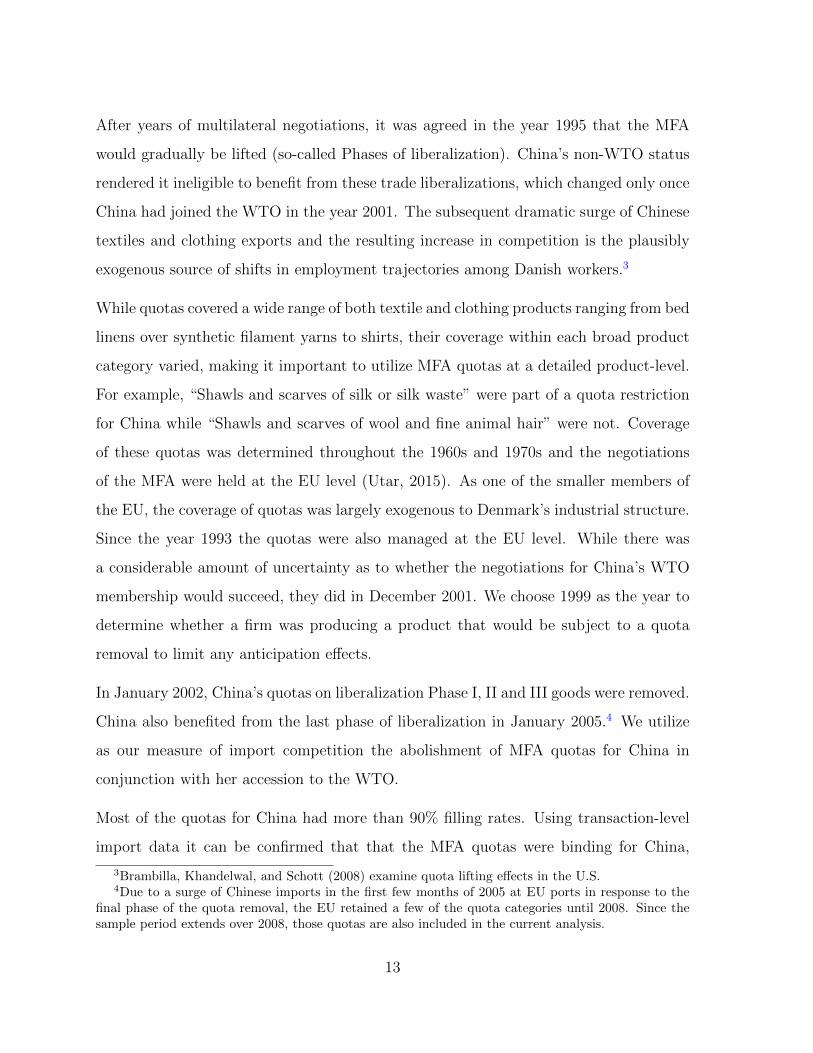
After years of multilateral negotiations, it was agreed in the year 1995 that the MFA
would gradually be lifted (so-called Phases of liberalization). China’s non-WTO status
rendered it ineligible to benefit from these trade liberalizations, which changed only once
China had joined the WTO in the year 2001. The subsequent dramatic surge of Chinese
textiles and clothing exports and the resulting increase in competition is the plausibly
exogenous source of shifts in employment trajectories among Danish workers.3
While quotas covered a wide range of both textile and clothing products ranging from bed
linens over synthetic filament yarns to shirts, their coverage within each broad product
category varied, making it important to utilize MFA quotas at a detailed product-level.
For example, “Shawls and scarves of silk or silk waste” were part of a quota restriction
for China while “Shawls and scarves of wool and fine animal hair” were not. Coverage
of these quotas was determined throughout the 1960s and 1970s and the negotiations
of the MFA were held at the EU level (Utar, 2015). As one of the smaller members of
the EU, the coverage of quotas was largely exogenous to Denmark’s industrial structure.
Since the year 1993 the quotas were also managed at the EU level. While there was
a considerable amount of uncertainty as to whether the negotiations for China’s WTO
membership would succeed, they did in December 2001. We choose 1999 as the year to
determine whether a firm was producing a product that would be subject to a quota
removal to limit any anticipation effects.
In January 2002, China’s quotas on liberalization Phase I, II and III goods were removed.
China also benefited from the last phase of liberalization in January 2005.4 We utilize
as our measure of import competition the abolishment of MFA quotas for China in
conjunction with her accession to the WTO.
Most of the quotas for China had more than 90% filling rates. Using transaction-level
import data it can be confirmed that that the MFA quotas were binding for China,
3Brambilla, Khandelwal, and Schott (2008) examine quota lifting effects in the U.S.4Due to a surge of Chinese imports in the first few months of 2005 at EU ports in response to the
final phase of the quota removal, the EU retained a few of the quota categories until 2008. Since thesample period extends over 2008, those quotas are also included in the current analysis.
13

and both the 2002 and the 2005 quota lifting caused a substantial surge of MFA goods,
accompanied by a decline in unit prices of these goods (Utar 2014).5 As a consequence,
virtually all workers employed at firms subject to the quota removals faced increased
import competition from China. We use the revenue share of firms in quota goods in
1999 as our measure of exposure to import competition. The results with a simple 0/1
indicator variable of whether a firm has any quota goods in its product mix or not are
very similar. It is also possible in this setting to employ a two-stage least squares strategy
in which exposure to quota removal is the instrument for rising import competition from
China; this leads to qualitatively very similar results (see Utar 2014).
3 Supplementary Information and Analysis
The following provides information on our breakdown into high-, mid-, and low-wage
occupations. Employing the classfication of Goos, Manning, and Salomons (2014) based
on two-digit occupations across 16 European countries (including Denmark) gives similar
results.
5Khandelwal, Schott, and Wei (2013) shows that the quota removal for China led to an extraefficiency gain in China due to prior mismanagement of quotas by the Chinese government and thedecline in prices were a result of entry of more efficient Chinese producers into the export market.
14

3.1 Variable Definitions and Descriptive Statistics
Table B-1: Characteristics of High-, Mid-, and Low Wage Occupations in 1999
Occupation Median Log % of workers with Employment CorrespondingClasses Hourly Wage at most High Share ISCO codes
School DiplomaLow-Wage 4.88 0.55 0.28 9 (except 92),5Mid-Wage 5.00 0.38 0.35 4,7,8High-Wage 5.22 0.14 0.37 1,2,3
Data are from 1999. Values are expressed in 2000 Danish Kroner. Employment share is measured asthe share of workers holding corresponding occupation as a primary attachment to the labor market withpositive hourly wage. Data Source: Statistics Denmark.
11.5
55
13.6
13
3.60
6
33.8
39
0.23
2
0.03
1
26.4
07
10.7
17
010
2030
40pe
rcen
t
Construction Financial and Business ServicesFood and Hospitality Serv. ManufacturingMining RecyclingTrade Services Transportation, Shipping, and Comm. Serv.
Figure 1: Industry Affiliation of Workers in 1999 in the Economy-Wide Sample (n =900,329)
Tables B-2 and B-3 give definitions and summary statistics as well as sources for all our
variables, respectively.
15

Tab
leB
-2:
Var
iable
defi
nit
ions
Vari
ab
leN
am
eV
ari
ab
led
efi
nit
ion
Fem
ale
Equ
alto
1if
wor
ker
isfe
mal
e,0
oth
erw
ise
Imm
igra
nt
Equ
al
to1
ifw
orke
ris
firs
tor
seco
nd
gen
erat
ion
imm
igra
nt,
0ot
her
wis
eA
ge
Wor
ker
’sag
ein
year
sas
of19
99C
olle
geE
qu
al
to1
ifw
orke
rat
ten
ded
aco
lleg
eas
of19
99,
0ot
her
wis
eV
oca
tion
al
Equ
alto
1if
hig
hes
tat
tain
eded
uca
tion
ofw
orke
ris
voca
tion
alsc
hool
asof
1999
,0
oth
erw
ise
Hig
hS
chool
Equ
al
to1
ifh
igh
est
atta
ined
edu
cati
onof
wor
ker
isa
gen
eral
hig
hsc
hool
asof
1999
,0
oth
erw
ise
Un
emp
loym
ent
His
tory
Su
mm
atio
nof
unem
plo
ym
ent
spel
lsof
wor
keri
unti
l19
99(e
xp
ress
edin
yea
rs)
Log
Hou
rly
Wag
eL
ogof
hou
rly
wag
eof
wor
ker
in19
99U
nio
nM
emb
ersh
ipE
qu
al
to1
ifw
orke
ris
am
emb
erof
au
nio
nin
1999
,0
oth
erw
ise
UI
Mem
ber
ship
Equ
alto
1if
wor
ker
isa
mem
ber
ofU
nem
plo
ym
ent
Insu
rance
(UI)
asof
1999
,0
other
wis
eE
xp
erie
nce
Nu
mb
erof
year
sw
orke
ri
isin
the
lab
orm
arke
tas
of19
99E
xp
erie
nce
2S
qu
are
of
Exp
erie
nce
Sep
ara
tion
Rate
Th
esh
are
of
wor
ker
sw
ho
are
not
emp
loye
din
the
firm
(of
wor
keri)
from
1998
to19
99L
ogF
irm
Wag
eL
ogar
ith
mof
aver
age
hou
rly
wag
epai
din
the
firm
(of
wor
keri)
in19
99F
irm
Siz
eT
he
full
-tim
eeq
uiv
alen
tnu
mb
erof
emp
loye
esin
the
firm
(of
wor
keri)
in19
99In
du
stry
Voca
tion
al
Lab
or
Sh
are
Th
ew
age
shar
eof
wor
kers
wit
hvo
cati
onal
sch
ool
edu
cati
onov
erth
eto
tal
wag
ep
aym
ent
inth
efo
ur-
dig
itin
du
stry
(of
wor
keri)
in19
99In
du
stry
ITIn
vest
men
tT
he
share
ofw
orke
rsw
ith
ITed
uca
tion
inth
e6-
dig
itin
du
stry
(of
wor
keri)
in19
99
Ind
ust
ryP
re-T
ren
dT
he
per
centa
gech
ange
bet
wee
n19
93-1
999
inth
eto
tal
nu
mb
erof
emp
loye
esin
wor
kers
’6-
dig
itin
du
stry
in19
99In
du
stry
Siz
eT
he
loga
rith
mof
the
nu
mb
erof
wor
ker
sem
plo
yed
inw
orke
ri’
ssi
xd
igit
ind
ust
ryin
1999
Ret
ail
Dem
an
dC
han
ge
Th
ep
erce
nta
geof
emp
loym
ent
chan
ges
over
2000
-200
8in
the
corr
esp
ond
ing
reta
il/w
hol
esal
ese
ctor
ofth
esi
x-d
igit
man
ufa
ctu
rin
gin
du
stry
ofw
orke
rE
ner
gyG
row
thT
he
aver
age
an
nu
algr
owth
inen
ergy
exp
end
itu
rein
the
fou
r-d
igit
ind
ust
ryov
er20
00-2
008
16

Table B-3: Variable Statistics
Variable Name Mean Standard
Deviation
Source
Female 0.339 0.473 IDA-personer
Immigrant 0.045 0.208 IDA-personer
Age 34.093 8.852 IDA-personer
College 0.176 0.381 IDA
Vocational 0.436 0.496 IDA
High School 0.377 0.485 IDA
Unemployment History 1.025 1.716 IDA-personer
Log Hourly Wage 5.032 0.448 IDA-ansættelser
Union Membership 0.762 0.426 Income registers
UI Membership 0.807 0.395 Income registers
Experience 12.868 6.205 IDA-personer
Experience squared 204.097 148.870 IDA-personer
Separation Rate 0.297 0.225 IDA-arbejdssteder
Log Firm Wage 5.121 0.247 IDA-arbejdssteder
Firm Size 231.863 668.347 IDA-arbejdssteder
Industry Vocational Labor
Share
0.461 0.144 IDA
Industry IT Investment 0.005 0.014 IDA
Industry Pre-Trend 0.278 0.713 IDA
Industry Size 8.713 1.250 IDA
Retail Demand Change 0.097 0.195 FIRE
Energy Growth -0.075 0.105 FIRE
∆IPCH 0.011 0.030 UHDI, FIRE
∆HIPCH 1.240 4.196 FIRE, EUROSTAT,
COMTRADE
Log distance to import
source
2.465 3.456 CEPII, UHDI
Share of retail firms in
import
0.020 0.052 UHDI, FIRE
17

Table B-4 gives the full two-stage least squares results that are summarized in Table 4
of the paper. At the bottom of Table B-4, the coefficients and standard errors of the
excluded instruments are shown.
Table B-4: Import Competition and Job Polarization
Dep. Var. HIGHe MIDe LOW e
(1) (2) (3)
∆IPCH 2.307* -5.273* 2.369*
(1.075) (2.282) (1.178)
Female -0.067 0.109 0.133*
(0.046) (0.075) (0.054)
Immigrant -0.559** −0.075◦ 0.025
(0.033) (0.039) (0.041)
Age -0.036** -0.021** -0.001
(0.003) (0.003) (0.003)
College 1.682** -0.407** -0.248**
(0.058) (0.065) (0.040)
Vocational 0.131** 0.471** 0.014
(0.029) (0.068) (0.049)
High School 0.104** 0.175** 0.070*
(0.033) (0.036) (0.028)
Unemployment History -0.118** -0.134** 0.032**
(0.008) (0.011) (0.006)
Log Hourly Wage 0.362** -0.317** -0.199**
(0.070) (0.047) (0.072)
Union Membership 0.028 0.554** 0.154**
(0.037) (0.057) (0.037)
UI Membership -0.324** 0.503** 0.317**
(0.093) (0.032) (0.065)
Experience 0.003 0.020 0.019
(0.006) (0.017) (0.014)
Experience squared 0.001* 0.002** -0.000
(0.000) (0.001) (0.001)
Separation Rate 0.051 -0.719** -0.047
(0.047) (0.063) (0.052)
Log Firm Wage 0.658** -0.000 -0.130*
(0.084) (0.095) (0.065)
Firm Size 0.000** -0.000** 0.000◦
(0.000) (0.000) (0.000)
Continued on next page
18
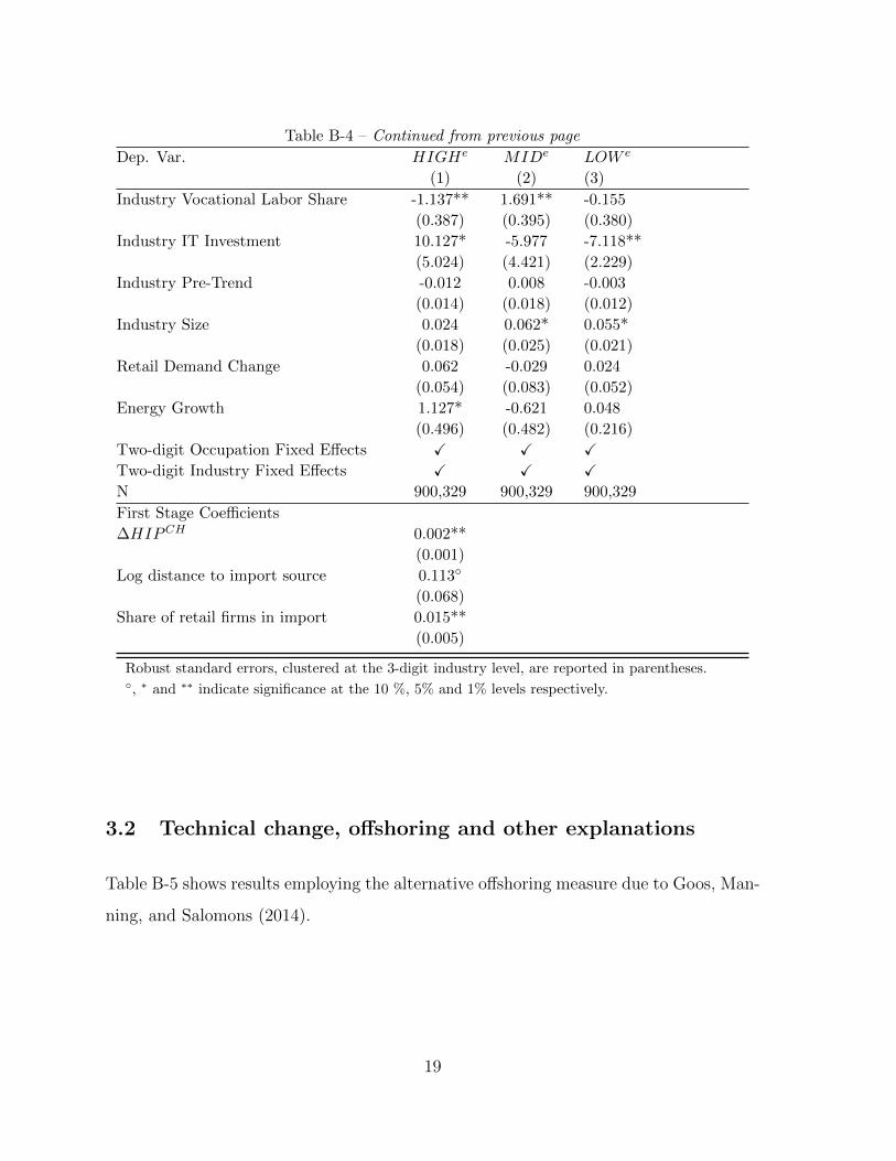
Table B-4 – Continued from previous page
Dep. Var. HIGHe MIDe LOW e
(1) (2) (3)
Industry Vocational Labor Share -1.137** 1.691** -0.155
(0.387) (0.395) (0.380)
Industry IT Investment 10.127* -5.977 -7.118**
(5.024) (4.421) (2.229)
Industry Pre-Trend -0.012 0.008 -0.003
(0.014) (0.018) (0.012)
Industry Size 0.024 0.062* 0.055*
(0.018) (0.025) (0.021)
Retail Demand Change 0.062 -0.029 0.024
(0.054) (0.083) (0.052)
Energy Growth 1.127* -0.621 0.048
(0.496) (0.482) (0.216)
Two-digit Occupation Fixed Effects X X XTwo-digit Industry Fixed Effects X X XN 900,329 900,329 900,329
First Stage Coefficients
∆HIPCH 0.002**
(0.001)
Log distance to import source 0.113◦
(0.068)
Share of retail firms in import 0.015**
(0.005)
Robust standard errors, clustered at the 3-digit industry level, are reported in parentheses.◦, ∗ and ∗∗ indicate significance at the 10 %, 5% and 1% levels respectively.
3.2 Technical change, offshoring and other explanations
Table B-5 shows results employing the alternative offshoring measure due to Goos, Man-
ning, and Salomons (2014).
19

Tab
leB
-5:
Job
Pol
ariz
atio
n,
Off
shor
ing,
Tec
hnol
ogy,
and
Tra
de–
Alt
ernat
ive
offsh
orin
gva
riab
le
JP
eJP
eJP
eLOW
eM
ID
eHIGH
e
(1)
(2)
(3)
(4)
(5)
(6)
∆Im
por
tsfr
om
Ch
ina
10.1
94**
10.5
81**
10.4
95*
2.58
9*-5
.435
*2.
471*
(3.9
14)
(3.9
78)
(4.1
07)
(1.3
08)
(2.5
08)
(1.2
21)
[0.0
43]
[0.0
45]
[0.0
45]
[0.
031]
[-0.
043]
[0.0
20]
Off
shor
ing
(GM
S)
0.09
5◦
0.00
80.
132*
*−
0.0
54◦
-0.1
78**
(0.0
48)
(0.0
40)
(0.0
17)
(0.0
28)
(0.0
20)
[0.
015]
[0.
001]
[0.
061
][
-0.0
16]
[-0.
055]
Rou
tin
eT
ask
Inte
nsi
ty0.
375*
*0.
008
-0.1
54*
0.21
2**
(0.1
11)
(0.0
35)
(0.0
62)
(0.0
43)
[0.
054
][
0.00
3][-
0.04
1]
[0.0
58]
Nu
mb
erof
Ob
serv
ati
on
s80
9,79
180
9,79
180
9,79
180
9,79
180
9,79
180
9,79
1F
-tes
tfi
rst-
stage
11.8
1711
.860
11.8
6611
.866
11.8
6611
.866
F-t
est
firs
t-st
age
[p-v
alu
e][0
.000
][0
.000
][0
.000
][0
.000
][0
.000
][0
.000
]
Note
s:E
stim
atio
nby
two
stag
ele
ast
squ
ares
.R
ob
ust
stan
dard
erro
rsare
rep
ort
edin
pare
nth
eses
.T
hey
are
clu
ster
edat
the
3-d
igit
ind
ust
ryle
vel.
Bet
aco
effici
ents
are
rep
orte
din
squ
are
bra
cket
s.A
llsp
ecifi
cati
on
sin
clu
de
dem
ogra
ph
ic(g
end
er,
age,
imm
igra
tion
statu
s),
edu
cati
on
,w
age,
lab
orm
arket
his
tory
(un
emp
loym
ent
his
tory
,li
nea
ran
dsq
uare
term
sof
exp
erie
nce
),u
nio
nan
du
nem
plo
ym
ent
insu
ran
cem
emb
ersh
ips,
firm
vari
able
s(s
ize,
wag
e,se
par
atio
nra
te),
asw
ell
as
pro
du
ct-l
evel
cova
riate
sas
inT
ab
le??.
All
spec
ifica
tion
sals
oin
clu
de
two-d
igit
ind
ust
ryfi
xed
effec
ts.
All
regr
essi
ons
incl
ud
eb
egin
nin
gofth
ep
erio
docc
up
ati
on
ind
icato
rsfo
rh
igh
-,m
id-,
an
dlo
w-w
age
occ
up
ati
on
san
dth
eocc
up
ati
on
s’li
keli
hood
ofin
tera
ctin
gw
ith
com
pu
ters
,va
ries
at
fou
r-d
igit
occ
up
ati
on
(fro
mO
*N
ET
).“O
ffsh
ori
ng
(GM
S)”
isth
eoff
shora
bil
ity
of
work
eri’
stw
od
igit
occ
up
atio
ncl
ass,
du
eto
Goos
,M
ann
ing
an
dS
alo
mon
s(2
014).
“R
ou
tin
eT
ask
Inte
nsi
ty”
foll
ows
Au
tor,
Lev
yan
dM
urn
an
e(2
003)
an
dA
uto
ran
dD
orn
(201
3);
itca
ptu
res
the
rou
tin
eta
skin
ten
sity
of
work
eri’
stw
od
igit
occ
up
ati
on
cod
e.T
he
sou
rce
of
the
off
shori
ng
an
dro
uti
ne
task
inte
nsi
tyva
riab
les
isG
oos
,M
ann
ing
and
Salo
mon
s(2
014).
Th
enu
mb
erof
ob
serv
ati
on
sd
rop
sb
ecau
seth
ere
are
no
routi
ne
task
inte
nsi
tyor
offsh
orin
gm
easu
res
for
som
eof
the
Dan
ish
occ
up
ati
on
cod
es.
◦ ,∗
an
d∗∗
ind
icate
sign
ifica
nce
at
the
10
%,
5%
an
d1%
leve
lsre
spec
tive
ly.
20

3.3 Within versus Between Shifts–A Quasi-Experiment
Table B-6 shows the importance of between-sector shifts for the textile quasi-natural ex-
periment. The results are similar to the corresponding Table 5 for Denmark’s entire econ-
omy.Table B-6: Within versus Between Shifts for 1999 Textile Workers
(1) (2) (3) (4)
Panel A. Mid-Wage Employment 2002-2009
MIDe MIDe MIDe MIDe
Within Outside Service
Manuf. Manuf. Sectors
Import Competition -1.513** -1.943** 0.430* 0.451*
(0.344) (0.393) (0.192) (0.189)
Panel B. High-Wage Employment 2002-2009
HIGHe HIGHe HIGHe HIGHe
Within Outside Service
Manuf. Manuf. Sectors
Import Competition 0.692** -0.323 1.015** 1.006**
(0.252) (0.249) (0.201) (0.200)
Panel C. Low-Wage Employment 2002-2009
LOW e LOW e LOW e LOW e
Within Outside Service
Manuf. Manuf. Sectors
Import Competition 0.746** 0.196 0.550** 0.549**
(0.205) (0.128) (0.168) (0.163)
Notes: N=10,487 in all regressions. Estimation by OLS. Import competition is defined as revenueshare of worker i’s firm in quota affected products. All specifications include demographic (gender,age, immigration status), hourly wage, education, labor market history (unemployment history, linearand square terms of experience), union and unemployment insurance memberships, firm variables (size,wage, separation rate), as well as two-digit occupation fixed effects. Robust standard errors are reportedin parentheses. They are clustered at the firm-level. ◦, ∗ and ∗∗ indicate significance at the 10 %, 5%and 1% levels respectively.
21

3.4 Trade, Tasks and Job Polarization
This section provides more detail on the results summarized in section 4.2 of the paper.
Our approach is to interact the import competition exposure variable with a measure of
the importance of a particular task in that worker i’s initial four-digit occupation class.
The regression of cumulative worker employment in 2002 to 2009 includes three terms,
in addition to all worker and firm variables employed in our analysis. The first two are
the linear trade and task measures, and the third is the interaction between trade and
task measure.
The analysis with O*NET tasks representative of routine manual tasks is given in Table
B-7, while results for non-routine manual tasks are shown in Table B-8; furthermore,
we show results for routine cognitive tasks in Table B-9 and for abstract tasks in Table
B-10.
22
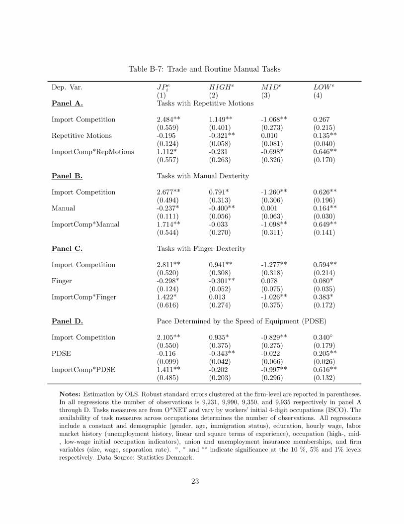
Table B-7: Trade and Routine Manual Tasks
Dep. Var. JP ei HIGHe MIDe LOW e
(1) (2) (3) (4)Panel A. Tasks with Repetitive Motions
Import Competition 2.484** 1.149** -1.068** 0.267(0.559) (0.401) (0.273) (0.215)
Repetitive Motions -0.195 -0.321** 0.010 0.135**(0.124) (0.058) (0.081) (0.040)
ImportComp*RepMotions 1.112* -0.231 -0.698* 0.646**(0.557) (0.263) (0.326) (0.170)
Panel B. Tasks with Manual Dexterity
Import Competition 2.677** 0.791* -1.260** 0.626**(0.494) (0.313) (0.306) (0.196)
Manual -0.237* -0.400** 0.001 0.164**(0.111) (0.056) (0.063) (0.030)
ImportComp*Manual 1.714** -0.033 -1.098** 0.649**(0.544) (0.270) (0.311) (0.141)
Panel C. Tasks with Finger Dexterity
Import Competition 2.811** 0.941** -1.277** 0.594**(0.520) (0.308) (0.318) (0.214)
Finger -0.298* -0.301** 0.078 0.080*(0.124) (0.052) (0.075) (0.035)
ImportComp*Finger 1.422* 0.013 -1.026** 0.383*(0.616) (0.274) (0.375) (0.172)
Panel D. Pace Determined by the Speed of Equipment (PDSE)
Import Competition 2.105** 0.935* -0.829** 0.340◦
(0.550) (0.375) (0.275) (0.179)PDSE -0.116 -0.343** -0.022 0.205**
(0.099) (0.042) (0.066) (0.026)ImportComp*PDSE 1.411** -0.202 -0.997** 0.616**
(0.485) (0.203) (0.296) (0.132)
Notes: Estimation by OLS. Robust standard errors clustered at the firm-level are reported in parentheses.In all regressions the number of observations is 9,231, 9,990, 9,350, and 9,935 respectively in panel Athrough D. Tasks measures are from O*NET and vary by workers’ initial 4-digit occupations (ISCO). Theavailability of task measures across occupations determines the number of observations. All regressionsinclude a constant and demographic (gender, age, immigration status), education, hourly wage, labormarket history (unemployment history, linear and square terms of experience), occupation (high-, mid-, low-wage initial occupation indicators), union and unemployment insurance memberships, and firmvariables (size, wage, separation rate). ◦, ∗ and ∗∗ indicate significance at the 10 %, 5% and 1% levelsrespectively. Data Source: Statistics Denmark.
23
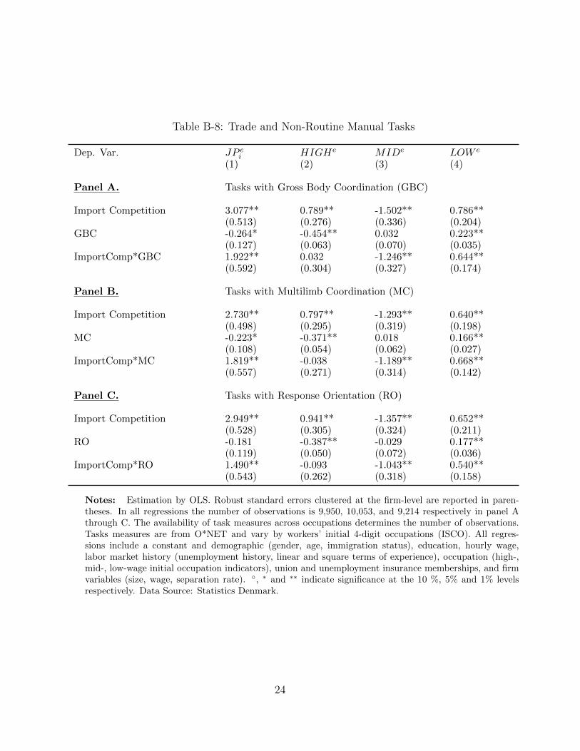
Table B-8: Trade and Non-Routine Manual Tasks
Dep. Var. JP ei HIGHe MIDe LOW e
(1) (2) (3) (4)
Panel A. Tasks with Gross Body Coordination (GBC)
Import Competition 3.077** 0.789** -1.502** 0.786**(0.513) (0.276) (0.336) (0.204)
GBC -0.264* -0.454** 0.032 0.223**(0.127) (0.063) (0.070) (0.035)
ImportComp*GBC 1.922** 0.032 -1.246** 0.644**(0.592) (0.304) (0.327) (0.174)
Panel B. Tasks with Multilimb Coordination (MC)
Import Competition 2.730** 0.797** -1.293** 0.640**(0.498) (0.295) (0.319) (0.198)
MC -0.223* -0.371** 0.018 0.166**(0.108) (0.054) (0.062) (0.027)
ImportComp*MC 1.819** -0.038 -1.189** 0.668**(0.557) (0.271) (0.314) (0.142)
Panel C. Tasks with Response Orientation (RO)
Import Competition 2.949** 0.941** -1.357** 0.652**(0.528) (0.305) (0.324) (0.211)
RO -0.181 -0.387** -0.029 0.177**(0.119) (0.050) (0.072) (0.036)
ImportComp*RO 1.490** -0.093 -1.043** 0.540**(0.543) (0.262) (0.318) (0.158)
Notes: Estimation by OLS. Robust standard errors clustered at the firm-level are reported in paren-theses. In all regressions the number of observations is 9,950, 10,053, and 9,214 respectively in panel Athrough C. The availability of task measures across occupations determines the number of observations.Tasks measures are from O*NET and vary by workers’ initial 4-digit occupations (ISCO). All regres-sions include a constant and demographic (gender, age, immigration status), education, hourly wage,labor market history (unemployment history, linear and square terms of experience), occupation (high-,mid-, low-wage initial occupation indicators), union and unemployment insurance memberships, and firmvariables (size, wage, separation rate). ◦, ∗ and ∗∗ indicate significance at the 10 %, 5% and 1% levelsrespectively. Data Source: Statistics Denmark.
24

Table B-9: Trade and Routine Cognitive Tasks
Dep. Var. JP ei HIGHe MIDe LOW e
(1) (2) (3) (4)
Panel A. Evaluating Information to Determine Compliance with Standards(Evaluating)
Import Competition 2.253** 0.492 -1.237** 0.523*(0.535) (0.330) (0.334) (0.243)
Evaluating 0.234◦ 0.025 -0.083 0.126**(0.121) (0.063) (0.065) (0.035)
ImportComp*Evaluating -1.669** −0.512◦ 0.590◦ -0.567*(0.592) (0.273) (0.302) (0.234)
Panel B. Importance of Repeating the Same Task (Repeating)
Import Competition 2.954** 0.758** -1.433** 0.763**(0.507) (0.281) (0.332) (0.208)
Repeating 0.121 0.227** 0.014 -0.092**(0.087) (0.040) (0.055) (0.031)
ImportComp*Repeating -1.329** -0.176 0.769** -0.384**(0.416) (0.199) (0.243) (0.147)
Notes: Estimation by OLS. Robust standard errors clustered at the firm-level are reported in parentheses. Inall regressions the number of observations is 10,364 and 9,986 respectively in panel A and B. The availabilityof task measures across occupations determines the number of observations. Tasks measures are from O*NETand vary by workers’ initial 4-digit occupations (ISCO). All regressions include a constant and demographic(gender, age, immigration status), education, hourly wage, labor market history (unemployment history,linear and square terms of experience), occupation (high-, mid-, low-wage initial occupation indicators),union and unemployment insurance memberships, and firm variables (size, wage, separation rate). ◦, ∗ and∗∗ indicate significance at the 10 %, 5% and 1% levels respectively. Data Source: Statistics Denmark.
25

Table B-10: Trade and Abstract Tasks
Dep. Var. JP ei HIGHe MIDe LOW e
(1) (2) (3) (4)
Panel A. Tasks that involve developing objectives and strategies (Strategy)
Import Competition 2.386** 0.926* -1.191** 0.268(0.568) (0.383) (0.313) (0.226)
Strategy 0.277* 0.150* -0.082 0.046(0.138) (0.061) (0.081) (0.042)
ImportComp*Strategy −1.086◦ 0.095 0.448 -0.733**(0.584) (0.265) (0.324) (0.205)
Panel B. Tasks that involve inductive thinking (Inductive)
Import Competition 2.196** 1.219** -1.025** -0.049(0.658) (0.468) (0.329) (0.241)
Inductive 0.202 0.219** -0.050 -0.068(0.152) (0.069) (0.083) (0.054)
ImportComp*Inductive −1.383◦ 0.456 0.723* -1.116**(0.716) (0.363) (0.339) (0.246)
Panel C. Tasks that involve mathematical thinking (Math)
Import Competition 2.473** 0.717* -1.239** 0.517**(0.501) (0.315) (0.312) (0.187)
Math 0.269* 0.285** -0.035 -0.051(0.116) (0.055) (0.059) (0.042)
ImportComp*Math -1.837** -0.150 0.872** -0.814**(0.514) (0.254) (0.256) (0.178)
Panel D. Tasks that involve making decisions (Decision)
Import Competition 2.385** 0.980* -1.225** 0.180(0.602) (0.417) (0.312) (0.245)
Decision 0.156 0.046 -0.036 0.074◦
(0.130) (0.057) (0.082) (0.038)ImportComp*Decision -0.933 0.110 0.352 -0.691**
(0.572) (0.279) (0.303) (0.214)
Notes: Estimation by OLS. Robust standard errors clustered at the firm-level are reported in parentheses.In all regressions the number of observations is 9,258, 9,803, 10,066, and 9,313 respectively in panels Athrough D. The availability of task measures across occupations determine the number of observations.Tasks measures are from O*NET and vary by workers’ initial 4-digit occupations (ISCO). All regressionsinclude a constant and demographic (gender, age, immigration status), education, hourly wage, labor markethistory (unemployment history, linear and square terms of experience), occupation (high-, mid-, low-wageinitial occupation indicators), union and unemployment insurance memberships, and firm variables (size,wage, separation rate). ◦, ∗ and ∗∗ indicate significance at the 10 %, 5% and 1% levels respectively. DataSource: Statistics Denmark.
26
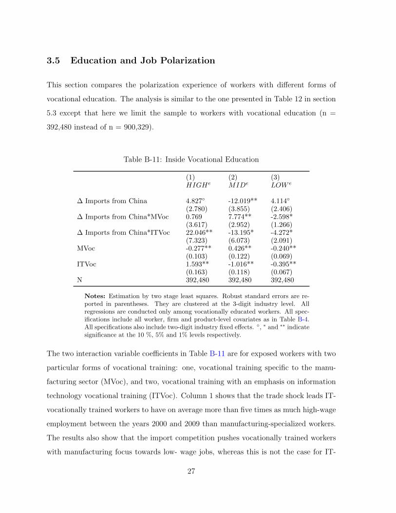
3.5 Education and Job Polarization
This section compares the polarization experience of workers with different forms of
vocational education. The analysis is similar to the one presented in Table 12 in section
5.3 except that here we limit the sample to workers with vocational education (n =
392,480 instead of n = 900,329).
Table B-11: Inside Vocational Education
(1) (2) (3)HIGHe MIDe LOW e
∆ Imports from China 4.827◦ -12.019** 4.114◦
(2.780) (3.855) (2.406)∆ Imports from China*MVoc 0.769 7.774** -2.598*
(3.617) (2.952) (1.266)∆ Imports from China*ITVoc 22.046** -13.195* -4.272*
(7.323) (6.073) (2.091)MVoc -0.277** 0.426** -0.240**
(0.103) (0.122) (0.069)ITVoc 1.593** -1.016** -0.395**
(0.163) (0.118) (0.067)N 392,480 392,480 392,480
Notes: Estimation by two stage least squares. Robust standard errors are re-ported in parentheses. They are clustered at the 3-digit industry level. Allregressions are conducted only among vocationally educated workers. All spec-ifications include all worker, firm and product-level covariates as in Table B-4.All specifications also include two-digit industry fixed effects. ◦, ∗ and ∗∗ indicatesignificance at the 10 %, 5% and 1% levels respectively.
The two interaction variable coefficients in Table B-11 are for exposed workers with two
particular forms of vocational training: one, vocational training specific to the manu-
facturing sector (MVoc), and two, vocational training with an emphasis on information
technology vocational training (ITVoc). Column 1 shows that the trade shock leads IT-
vocationally trained workers to have on average more than five times as much high-wage
employment between the years 2000 and 2009 than manufacturing-specialized workers.
The results also show that the import competition pushes vocationally trained workers
with manufacturing focus towards low- wage jobs, whereas this is not the case for IT-
27

educated workers. IT-education helps in two ways, by increasing the chance of moving to
high-wage jobs and by reducing the likelihood of moving down to low-wage employment.
28
![Lessons from Reducing Emissions from Deforestation and ... › giee › pubpdfs › Negra_2011_Carbon... · Under the UN Framework Convention on Climate Change (UNFCCC) [101], coun-tries](https://img.pdfslide.net/doc/110x75/5f03bdec7e708231d40a8b55/lessons-from-reducing-emissions-from-deforestation-and-a-giee-a-pubpdfs.jpg)