Embed Size (px)
Citation preview

Trade Costs
James E Anderson Eric van Wincoop
Journal of Economic Literature Vol 42 No 3 (Sep 2004) pp 691-751
Stable URL
httplinksjstororgsicisici=0022-05152820040929423A33C6913ATC3E20CO3B2-23
Journal of Economic Literature is currently published by American Economic Association
Your use of the JSTOR archive indicates your acceptance of JSTORs Terms and Conditions of Use available athttpwwwjstororgabouttermshtml JSTORs Terms and Conditions of Use provides in part that unless you have obtainedprior permission you may not download an entire issue of a journal or multiple copies of articles and you may use content inthe JSTOR archive only for your personal non-commercial use
Please contact the publisher regarding any further use of this work Publisher contact information may be obtained athttpwwwjstororgjournalsaeahtml
Each copy of any part of a JSTOR transmission must contain the same copyright notice that appears on the screen or printedpage of such transmission
The JSTOR Archive is a trusted digital repository providing for long-term preservation and access to leading academicjournals and scholarly literature from around the world The Archive is supported by libraries scholarly societies publishersand foundations It is an initiative of JSTOR a not-for-profit organization with a mission to help the scholarly community takeadvantage of advances in technology For more information regarding JSTOR please contact supportjstororg
httpwwwjstororgFri Nov 2 163131 2007
Journal of Economic Literature Vol XLII (September 2004) pp 691-751
Trade Costs
JAMES E ANDERSONand Eric van wincoop1
the report of m y death was a n exaggeration - Mark Twain 1897
1 Introduction
The death of distance is exaggerated Trade costs are large even aside from
trade-policy barriers and even between apparently highly integrated economies Despite many difficulties in measuring and inferring the height of trade costs and their decomposition into economically useful components the outlines of a coherent pic- ture emerge from recent developments in data collection and especially in structural modeling of costs Trade costs have econom- ically sensible magnitudes and patterns across countries and regions and across goods suggesting useful hypotheses for deeper understanding This survey is a progress report Much useful work remains to be done so we make suggestions below
Trade Costs Mattel (1)They are large-a 170-percent total trade barrier is construct- ed below as a representative rich country ad-valorem tax equivalent estimate This includes all transport border-related and local distribution costs from foreign poduc- er to final user in the domestic county (2)
klderson Boston College and NBER van Wincoop University of Virginia and NBER We are grateful to John McMillan two referees and Jeff Bergstrand for excep tionally generous and detailed comments and sugges- tions We have also benefitted from many other comments by colleagues too numerous to single out tllrough e-mail and in presentations at conferences and at university workshops
Trade costs are richly linked to economic policy Direct policy instruments (tariffs the tariff equivalents of quotas and trade barri- ers associated with the exchange-rate sys- tem) are less important than other policies (transport infrastructure investment law enforcement and related property-rights institutions informational institutions regu- lation language) (3) Trade costs have large welfare implications For example Anderson and van Wincoop (2002) argue that current policy-related costs are often worth more than 10 percent of national income (4) Maurice Obstfeld and Kenneth Rogoff (2000) argue that all the major puz- zles of international macroeconomics hang on trade costs ( 5 )Details of trade costs mat- ter to economic geography For example the home market effect hypothesis (big coun- tries produce more of goods with scale economies) hangs on differentiated goods with scale economies having greater trade costs than homogeneous goods (Donald Davis 1998) (6)The cross-commodity struc- ture of policy barriers is important to welfare i e ~ Anderson 1994)
i road lu ~ e f i n e d Trade costs broadlvJ J
defined include all costs inconed in getting a good to a other than Ihe margin- al cost of producing the good itself trans- portation costs (both freight costs and tirne
policy barriers itariffs and llontariff
barriers) information costs contract
Jozrrnal of Economic Litel
enforcement costs costs associated with the use of different currencies legal and regula- tory costs and local distribution costs (wholesale and retail) Trade costs are reported in terms of their ad-valorem tax equivalent The 170-percent headline num- ber breaks down into 55-percent local distri- bution costs and 74-percent international trade costs (17=155174-1)
Both domestic and international trade costs are included because it is arbitrary to stop counting trade costs once goods cross a border It is not even obvious when goods cross a border in the economic sense Is it when they arrive on the dock leave the dock arrive it the importer
Costs broadlv defined and reported below may include sonle rent Exclusion of rent requires a markup theory and its application
Tlzree Sorlrces We report on trade costs from three broad sources Direct measures of trade costs are discussed in section 2 Direct measures are remarkably sparse and inaccurate Two types of indirect measures complement the incomplete and inade-quate direct measures inference from quantities (trade volumes) discussed in sec- tion 3 and inference from prices discussed in section 4
Theory Looriw Large In our survey theo- n7looms large A theoretical approach is inevitable to infer the large portion of trade costs that cannot be directly measured in the data The literature on inference about trade barriers from final goods prices remains largely devoid of theory lie point to ways in which trade theory can be effectively used to fill this gap and learn more about trade bar- riers from evidence on prices Recent devel- opments have bridged the gap between practice and theory in the inference of trade costs from trade flows Readers who pause with us on the bridge will produce better work in the future
The gravity model provides the main link between trade barriers and trade flows Gravity is often taken to be rather atheoret- ic or justified only under highly restrictive
ratzrre Vol XLII (September 2004)
assumptions We place gravity in a wide class of trade separable general equilibrium mod- els Trade separability obtains when the allo- cation of trade across countries is separable from the allocation of production and spending within countries Gravity links the cross-country general equilibrium trade allocation to the cross-country trade barri- ers all conditional on the observed con-sumption and production allocations Inferences about trade costs therefore do not depend on the general equilibrium structure that lies beneath the observed consumption and production allocations within countries
Appropriate aggregation of trade costs is a key concern Aggregation of some sort is inevitable due both to the coarseness of observations of complex underlying phe- nomena and the desirability of simple meas- ures of very high dimensional information lie show how theory can be used to replace common atheoretic aggregation methods with ideal aggregation lie also show how theory can shed light on aggregation bias and what can be done to resolve it
Trade Costs Are Large and Variable Mattels Barbie doll discussed in Robert Feenstra (1998) illustrates large costs The production costs for the doll are $1 while it sells for about $10 in the United States The cost of transportation marketing wholesal- ing and retailing have an ad-valorem tax equivalent of 900 percent
A rough estimate of the tax equivalent of representative trade costs for industrialized countries is 170 percent This number breaks down as follows 21 percent transportation costs 44 percent border-related trade barri- ers and 55 percent retail and wholesale dis- tribution costs (27=121 144155) The 21-percent transport cost includes both directly measured freight costs and a 9-per- cent tax equivalent of the time value of goods in transit Both are based on estimates for US data The 44-percent border-related barrier is a combination of direct observation and inferred costs Total international trade
693 Anderson and van Wincoop Trade Costs
costs are then about 74 percent (074=121144-1) Representative retail and wholesale distribution costs are set at 55 percent close to the average for industrial- ized countries
Direct evidence on border costs shows that tariff barriers are now low in most countries on average (trade-weighted or arithmetic) less than 5 percent for rich countries and with a few exceptions are on average between 10 percent and 20 percent for developing countries Our overall repre- sentative estimate of policy barriers for industrialized countries (including nontariff barriers) is about 8 percent Inferred bor- der costs appear on average to dwarf the effect of tariff and nontariff policy barriers An extremely rough breakdown of the 44-percent number reported above is as follows an 8-percent policy barrier a 7-percent language barrier a 14-percent currency barrier (from the use of different currencies) a 6-percent information cost barrier and a 3-percent security barrier for rich countries
Trade costs are also highly variable across both goods and countries ampade barriers in developing countries are higher than those reported above for industrialized countries High value-to-weight goods are less penal- ized by transport costs The value of timeli- ness varies across goods explaining modal choice Poor institutions and poor infrastruc- ture penalize trade differentially across countries Sectoral trade barriers appear to vary inversely with elasticities of demand Policy barriers especially nontariff barriers (NTBs) also vary significantly across goods NTBs are highly concentrated in many sec- tors they are close to zero but US textiles and apparel have 71 percent of products covered with tariff equivalents ranging from 5 percent to 33 percent
2 Direct Evidence
Direct evidence on trade costs comes in two major categories costs imposed by
policy (tariffs quotas and the like) and costs imposed by the environment (trans- portation insurance against various haz- ards time costs) We review evidence on international policy barriers transport costs and wholesale and retail distribution costs We focus on current and recent trade costs in this survey see the work of Williamson and co-authors (eg Kevin ORourke and Jeffrey Williamson 1999) for historical evidence
An important theme is the many difficul- ties faced in obtaining accurate measures of trade costs Particularly egregious is the paucity of good data on policy barriers Transport-cost data is limited in part by its private nature Many other trade costs such as those associated with information barriers and contract enforcement cannot be direct- ly measured at all Better data on trade costs are feasible with institutional resources and would yield a high payoff
21 Policy Barriers
211 Measurement Problerns and Limitations
How high are policy barriers to trade This seemingly simple question cannot usu- ally be answered with accuracy for most goods in most countries at most dates The inaccuracy arises from three sources absence of data data that are useful only in combination with other missing or fragmen- tary data and aggregation bias Each of the difficulties is discussed further below
The key open3 (to the research communi- ty) source for panel data on policy barriers
he grossly inco~nplete and inaccurate informatioll on policy barriers available to researchers is a scandal and a puzzle It is natural to assume that trade policy is well- documented since theoq and politics have emphasized it for hundreds o f years
UNCTAD sells the TRAINS data each year to com- ~nercial custo~ners who use it to provide current informa- tion on trade costs to potential traders It comes with a front end designed for convenience in pulling a maxi~nu~n o f 200 lines o f data while preventing a user from gaining access to the whole database and using it to compete with UNCTADs potential sales to other customers
694 Journal of Economic Literature Vol XLII (September 2004)
to trade is the United Nations Conference on Trade and Developments Trade Analvsis amp Information System TRAINS It contains information on trade control measures (tar- iff para-tarifp and nontariff measures) at tariff line level for a maximum of 137 coun- tries beginning in the late 1980s TRAINS reports all data on bilateral tariffs nontariff barriers and bilateral trade flows at the six- digit level of the Harmonized System (HS) product classification for roughly 5000 products Countries use a finer product classification when reporting tariffs to UNCTAD Thus multiple tariff lines underlie each six-digit aggregate It is in some cases possible to drill down to the national tariff line level Some organizations have obtained the full TRAINS database (without the front end software) and pro- vide access to a limited set of users inside the ~ r ~ a n i z a t i o n ~
Table 1 gives a sense of the substantial incompleteness of TRAINS For each year from 1989 to 2000 the table reports the fraction of countries that report some lines (though possibly a very limited number) for tariffs NTBs and trade flows Of 121 reporting countries in 1999 43 percent report tariffs 30 percent report NTBs 55 percent report trade flows and 174 per- cent have data for all three The other coun- tries report no data at all for any good Coverage is not much better in other ears Coverage is better for OECD countamp- over 50 percent have tariff and NTB infor- mation recorded in 1999 with considerable variability in coverage across the years
The World Bank has very recently put together from these elements the most
Para-tariff measures include customs surcharges such as i ~ p o r t license fees foreign exchange taxes stamps etc
For example Boston College has purchased disaggrr- gated tariff information from UNCTADs TRAINS data- base for the years 1988 through 2001 inclusi~e Ve havr data for 137 countries for at least one year counting the European Union as a single countq but far less than the maximum amount suggested by fourtren years timrs 137 countries
comprehensive svstem for researchers and in principle prdvides public Itsa c ~ e s s ~ World Integrated Trade System (WITS) sofhvare is coupled to TRAINS and to the World Trade Organization (WTO) Integrated Data Base and Consolidated Tariff ~chedules along with the UN Statistical Divisions COMTRADE trade flow data In principle it allows users to drill down and select data according to their own criteria to track the complexities of trade policy as finely as the primary inputs allow8 WITS has some other data handling and modeling functions as well
National sources in combination with the above allow better measurement of a single countrys trade policy A series from the Institute for International Economics pro- vides measures of a few national trade policies
see httpwitsworldbankorg At this writing there are still technical glitches facing a user tning to gain access I7ITS only runs in late model Untiows machines users may need some IT support to install the software and a user must to pay fees to UKCTAD for use of COM- TRADE and TRAINS Email queries are not answered in our experience without using friends at the Bank as inter- mediaries
The I T 0 Consolidated Tariff Schedule database lists the Most Favored Nation (MFN) boullti tariffs at the tar- iff line level The bound tariffs are the upper li~nits under the member countries I T 0 obligatioll for actual tariffs charged to countries not the~ n e ~ n b e r associated with importer in a free trade agreement or a customs union anti often exceed the actual duties charged The TOS Integrated Data Base colltaills information on the applied rates at the national tariff line level The tiata is closed to resrarchers The LIT0 periodically reports on indilidual member-counti trade policy with a published trade poli- cy review based on its data The 170rld Bank Trade allti Production database pro- duces from its resources a set of three- and four-digit aggregates of trade production and tariff data It is pub- lished on the Bank website and presumably will be regu- larly updated The Trade and Production database covers 67 developing and developrd countries over the period 1976-99 Again the tiescriptioll given misleadingly sug- grsts a usrful panel the actual data is full of missing obser- vations due to the untierling limitations of TRAINS The sector disaggregation in the database follows the Illtemational Standard Industrial Classification (ISIC) and is prolided at the three-digit level (28 industries) for 67 coulltries and at the four-digit level (81 industries) for 24 of thesr countries
Anderson and van Wincoop Trade Costs
TABLE 1 PERCENTAGEOF COUKTRIESWITH DATAIN TRAINS
All Countries OECD Countries Year Tariff NTB Trade All Tariff NTB Trade All
1989 08 17 17 08 00 00 56 00
2000 364 25 00 00 556 556 00
Notes The data are from UNCTADs TRAINS database (Haveman Repackaging) The table reports the percentage of all countries based on total of 121 reporting countries that have at least one type of data for one year available through TRAINS For OECD countries the percentages are based on 19 countries All indicates that a country has reported all three types of data for that year
for single years9 See also the WTOs Trade and must be converted to ad valorem equiv- Policy Reviews series alents using price information that must be
Data limitations can make even the avail- matched up to the tariffs Imperfections of able trade-barrier information difficult to classification or other information introduce interpret TRAINS does not routinely report potential measurement error TRAINS ad-valorem equivalents of specific tariffs (on reports the percentage of underlying lines quantities rather than values) Where specif- that have specific tariffs in order to provide ic tariffs are prevalent such as in agriculture some information about how widespread in many countries the omission of specific the measurement problem may be The tariffs is highly misleading Many tariffs are World Banks trade-barrier database sub- in the form of specific taxes (on quantity) stantially supplements TRAINS by supply-
ing missing specific tariff information The
See Gaq- Hufbauer and Kimberly Ann Elliott (1994) match of the tariff line classifications with on the United States Patrick Messerlin (2001) on the the commodity classifications for trade flows European Union Yoko Sazana~ni Shujiro Urate and is imperfect as well introducing measure- Hiroki Kawai (1995) on Japan Namdoo Kiln (1996) on South Korea and Shuguang Zhang Zhang Yansheng and ment error when converting all data to the Wan Zhonpn (1998)on China Harmonized System
00
696 Jou~malof Econoinic Literature Vol X L I I (Septeinber 2004)
Nontariff barriers (NTBs) are much more problematic than tariff barriers The World Bank database unfortunately does not pro- vide NTB data A user must use TRAINS or more specialized databases directed at par- ticular NTBs The TRAINS database records the presence or absence of a nontar- iff barrier (NTB) on each six-digit line Manv differing types of nontariff barriers ark recorded in TRAINS (a total of eighteen types) The NTB data requires concordance between the differing NTB tariffs and trade classification svstems at the national level converting to the common HS system
Jon Havemans extensive work with TRAINS has produced a usable NTB data- base Haveman follows what has become a customary grouping of NTBs into hard bar- riers (price and quantity measures) threat measures (antidumping and countervailing duty investigations and measures) and qual- ity measures (standards licensing require- ments etc) A fourth category is embargoes and prohibitions A common use of the NTB data is to construct a measure of the preva- lence of nontariff barriers such as the per- centage of HS lines in a given aggregate that are covered by NTBs Nontariff barrier information in TRAINS is particularly prone to incompleteness and poor-quality problems so analysts seeking to study parti- cular sectors such as the Multi-Fibre Arrangement (MFA) will do better to access specialized databases such as the World Banks MFA data
No information about NTB restrictive-ness is provided in TRAINS since measur- ing the restrictiveness of each type of nontariff barrier requires an economic model In some important cases individual analysts have developed direct measures of
lo See the Ultimate Trade Barrier Catalog at ht m~~veiitorgProtection
Uationd tmff line infornlation is also very problem- atic when analyzing nontariff barriers For example matching up reported trade flows with annual quotas immediateb runs into inconsistencies in reporting conven- tions
the restrictiveness of NTBs based on quota license prices where these are available
Indirect methods of measuring the restric- tiveness of NTBs are important because of the paucity of direct measures One method is to infer the restrictiveness of nontariff bar- riers through the comparison of prices Some important trade lines are well-suited for price comparisons (homogeneous products sold on well-organized exchanges for example) but even here there are important issues with domestic transport and intermediary margins and the location of wholesale markets rela- tive to import points of entry Evidence from price comparisons is discussed in section 4 The restrictiveness of nontariff barriers can also be inferred from trade quantities in the context of a well-specified model of trade flows Inference about nontariff barriers from trade flows is discussed in section 3 Alan Deardorff and Robert Stern (1998) and Sam Laird and Alexander Yeats (1990) pro- vide other detailed discussions of inference about the restrictiveness of NTBs
Aggregation is an important problem in the use and analysis of trade barriers Tariffs and NTBs comprise some 10000 lines with large variation across the lines The national customs authorities are the primary sources of trade restrictions and their classification systems do not match up internationally or even intranationally as between trade flows on the one hand and tariff and nontariff- barrier classes on the other hand Matching up the tariff nontariff and trade-flow data requires aggregation guided by concor-dances that are imperfect and necessarily generate measurement error Moreover for many purposes of analysis the comprehen- sion of the analyst is overwhelmed by detail and further aggregation is desirable Atheoretic indices such as arithmetic (equal- ly weighted) and trade-weighted average tar-
iffs are commonly used while production-weighted averages sometimes replace them for nontariff barriers the
indicator is aggregated into a nontar-iff barrier coverage ratio the arithmetic or
697 Anderson and van Wincoop Trade Costs
trade-weighted percentage of component sectors with nontariff barriers
Ideal aggregation is proposed by James Anderson and Peter Neary (1996 2003) based on the idea of a uniform tariff equiva- lent of differentiated tariffs and NTBs Theoretically consistent aggregation depends on the purpose of the analysis so the analyst must specify tariff equivalence with reference to an objective that makes sense for the task at hand Anderson and Neary develop and apply indices for the small-country case that are equivalent in terms of welfare and in terms of distorted aggregate trade volume12 and show that atheoretic aggregation can significantly bias the measurement of trade restrictiveness13 The theme of appropriate aggregation in the different setting of many countries in gener- al equilibrium plays a prominent role in our discussion of indirect measurement of trade costs so we defer a full treatment to that section Ideal aggregation is informationally demanding so for that reason and because of their familiarity and availability in the work of others we report the standard trade- weighted and arithmetic averages of tariffs and of NTB coverage ratios below
212 Evidence on Policy Barriers
Tariffs Trade-weighted and arithmetic average tariffs are reported in table 2 for fifty
ee also Anderson (1998)for equivalence in terms of sector-specific factor income and its relationship to the com~nonly reported effective rate of protection
l3Anderson and Neaq (2003)report results using a volu~ne equivalent uniform tariff- replacement of the dif- ferentiated tariff structure with a uniform tariff such that the general equilibrium aggregate value of trade in tiistort- eti products (in terms of external prices) is held constant The ideal index is usually larger than the trade-weighted average-an arithmetic average across countries in the study ields approximately 11percent for the trade weight- ed average anti 12 percent for the uniform volume equiv- alent while the US nu~nbers in 1990 are 4 percent and 48 percent respectively For purposes of co~nparison between the initial tariffs and free trade the two indexes are quite highly correlated For a s~naller set of evaluations of year-on-year changes in contrast Anderson anti Neal show that the ideal and trade-weighted average indexes are uncorrelatect
countries for 1999 based on TRAINS data14 The relatively small number of coun- tries reflects reporting difficulties typical of TRAINS some earlier years contain data for more countries The reported numbers aggregate the thousands of individual tariff lines in the underlying data The table con- firms that tariffs are low among most devel- oped countries (under 5 percent) while developing countries continue to have high- er tariff barriers (mostly over 10 percent) Dispersion across countries is wide Hong Kong and Switzerland have 0 percent tariffs the United States has a 19 percent simple average and at the high end India has 301 percent and Bangladesh 227 percent
The variation of tariffs across goods is quite large in all countries typically only a few are large Intuition suggests that the variation of tariffs adds to the welfare cost Marginal deadweight loss is proportional to the tariff hence the cumulated dead weight loss triangle varies with the square of the tar- iff Coefficients of variation (the ratio of the standard deviation to the mean) of tariffs either arithmetic or trade-weighted thus sometimes supplement averages Anderson and Neary (2003) report trade-weighted coefficients of variation of tariffs for 25 coun-tries around the year 1990 ranging from 014 to 167 many being clustered around one Thev show that a proper analysis quali- fies the simple intuition considerably with welfare cost increasing in an appropriately weighted coefficient of variation
Bilateral variation of tariffs can also be large Preferential trade is mainly responsible since insiders face a zero tariff while outsiders face the MFN tariff but aggregation over goods induces further bilateral variation due to differing composition of trade across part- ners James Harrigan (1993) reports bilateral production-weighted average tariffs in 28 product categories for OECD countries for
dculations were based on TRAINS annual data- bases purchased by Boston College without the front- e d software and assembled into panel data
TABLE 2 SILIPLE TARIFFAKD TRADE-VEIGHTED A V E R A G E S - ~ ~ ~ ~
County Simple T V Average Average
Argentina 148 113 Australia 45 41 Bahamas 07 08 Bahrain 78 -Bangladesh 227 218 Barbados 192 203 Belize 197 149 Bhutan 153 -
Boli~ia 97 91 Brazil 155 123 Canada 45 13 (bile 100 100 (oloinbia 122 107 (osta Rica 65 40 (zech Republic 55 -
Ilorninica 185 158 Ecuador 138 111 European Union 34 27 (korgia 106 -
Grenada 189 157 Guyana 207 -
Ilonduras 75 78 Hong Kong 00 00 India 301 -
Illdonesia 112 -
Jiiunaica 188 167
Japan 24 29 Korea 91 59 Mexico 175 66 hlontserrat 180 -
New Zealand 24 30 Nicaragua 105 110 Paraguay 130 61 Peru 134 126 Pllilippilles 97 -
Romania 159 83 Saudi Arabia 122 -
Singapore 00 00 Slovenia 98 114 Soutll Africa 60 44 St Kitts 187 -
St Lucia 187 -
St Uncent 183 -
Suriname 187 -
Switzerland 00 00 Taiwan 101 67 Trinidad 191 170 Ur11gua)i 49 45 USA 29 19 Ve~~ezuela 124 130
Xotcs Tlle data are from UNCTADs TRAINS database (Haveman repackagmg) A -indicates that trade data for 1999 are ullavailable in TRAINS
699 Anderson and van Wincoop Trade Costs
1983 For Canada the reported range of bilateral averages runs from 12 percent to 32 percent and for Japan from 23 percent to 45 percent The United States has more modest differences from 16 percent to 23 percent15
Nontarif Barriers Table 3 reports the prevalence of nontariff barriers for 34 coun- tries in 1999 based on data from TRAINS and Havemans work (rendering it more usable) The smaller number of countries available than for tariffs reflects previously noted limi- tations of TRAINS We report arithmetic and trade-weighted NTB coverage ratios the per- centage of tariff lines subject to NTBs The trade-weighted NTB coverage ratios general- ly exceed the arithmetic average NTB cover- age ratios often considerably so For example on the narrow definition (defined below) the US arithmetic NTB coverage is 15 percent while the trade-weighted NTB coverage is 55 percent This reflects the fact that NTBs tend to fall on important traded goods such as textiles and apparel
Narrow NTB coverage is basically price and quantity control measures and quality control measures while broad coverage is the narrow classification plus threat measures related to antidumping Threats are signifi- cant since Robert Staiger and Frank Wolak (1994) have shown that the threat of antidumping impedes trade considerably (on average for the United States they find a sev- enteen-percent reduction in trade due to an ongoing investigation) Narrow NTBs cover less than 10 percent of trade for the rich countries and modest amounts of trade in most except for Argentina and Brazil Table 3 implies that antidumping is quite common For example based on the TRAINS data the United States in 1999 had 15 percent of tar- iff lines subject to NTB when narrowly defined but 272 percent of tariff lines subject
l5 Harrigans data is available to the public Huiwen Lai and Daniel Trefler (2002) are notable for compiling three- digit bilateral tariffs for fourteen importers and 36 exporters for 1972 1977 1982 1987 and 1992 They emphasize the hard work involved and have not yet made the data public
to NTB when broadly defined These meas- ures do not include withdrawn suits which are presumptively restrictive since they facil- itate collusion Table 3 also shows wide vari- ability over countries in the use of NTBs The broad definition with arithmetic averages has South Africa at 113 percent and Argentina at 718 percent
The use of NTBs is concentrated in a few sectors in most economies Table 4 reports sectoral NTB coverage ratios for the United States European Union Japan and Canada for 1999 NTBs are widely used by devel- oped countries in food products (for exam- ple the trade-weighted NTB coverage of agriculture forestry and fishery products is 74 percent for the United States and 24 per- cent for the European Union) textilesappar- el (71 percent for the United States and 42 percent for the European Union) wood and wood products (39 percent for the United States and 26 percent for the European Union) and in some other areas of manufac- turing The products involved are quite sig- nificant in the trade of developing countries but also somewhat significant in the trade of developed countries with each other
In comparison to tariffs NTBs are con- centrated in a smaller number of sectors and in those sectors they are much more restric- tive Deardorff and Stern (1998) survey most of what limited data is available on quota license prices Table 5 (based on table 36 of Deardorff and Stern 1998) gives estimates of tax equivalents based on annual averages of week1 Hong Kong MFA quota license
(which are themselves averages of
l6Where markets subject to quotas are thick and well- organized and behavior of all agents is competitive quota license prices provide the best evidence of tariff equiva- lents Using license price data even under these assump- tions forces the analyst to face the many dimensions on which the quota is not equivalent to a tariff-daily price quotes exhibit within-year variation with economically sig- nificant patterns (seasonality year-end jumps and drops)- such that no single index of them can generally be equivalent to a tariff Nevertheless average license prices in combination with the substantial rent-retaining tariffs found on most quota-constrained products provide a use-ful measure of the restrictiveness of quotas
TABLE 3 NOY-TARIFFB R R I E R S - ~ ~ ~ ~
NTB ratio Tf7NTB ratio NTB ratio Tf7NTB ratio (narrow) (narrow) (broad) (broad)
Algeria
Argentina
Australia
Ballrain
Bhutan
Bolivia
Brazil
Canada
Chile
Colombia
Czech Republic
Ecuador
European Union
Guatemala
H u n g a ~
Indonesia
Lebanon
Lithuania
Mexico
Morocco
New Zealand
Oman
Paraguay
Peru
Poland
Romania
Saudi Arabia
Slo-enia
South Africa
Taiwan
Tunisia
Uruguay
USA
Venezuela
Xotes Tlle data are from UNCTADs TRAINS database (Haveman repackaging) Tlle narrow cat ego^ includes quantity price quality and ad-ance payment NTBs but does not include threat measures such as antidumping in-estigations and duties The broad categon includes quantity price quality advance payment and threat measures Tlle ratios are calculated based on six-digit HS categories 4 - indicates that trade data for 1999 are not available
Anderson and van Wincoop Trade Costs
TABLE 4 NTH COVERAGE RATIOSBY SECTOR-^^^^
United States 1999 EU-12 1999 Japan 1996 Canada 1999
Narrow Broad Narrow Broad Narrow Broad Narrow Broad
NTB-ratio NTB-ratio NTB-ratio KTB-ratio KTB-ratio KTB-ratio NTB-ratio NTB-ratio
ISIC Description 1 Agric Forestry Fish 011 052 719 743 001 001 229 241 153 227 897 962 028 022 878 938
2 Mining Quarcng 000 000 018 099 001 055 001 055 028 008 193 706 000 000 027 014
21 Coal Mining 000 000 000 000 004 000 004 000 000 000 667 1000 000 000 000 000
22 Crude Petroleum 000 000 250 105 004 067 004 067 000 000 1000 1000 000 000 375 019
23 Metal Ore Mining 000 000 000 000 000 000 000 000 087 000 087 000 000 000 000 000
29 Other Mining 000 000 000 000 001 038 001 038 014 129 120 184 000 000 000 000
3 Manufacturing 015 047 245 423 007 042 083 107 044 102 322 366 171 044 261 196
31 Food Bev Tobacco 072 120 644 809 004 011 489 474 185 329 925 893 185 348 456 453 32 Textiles Apparel 000 002 509 708 030 255 102 420 022 050 163 120 762 681 816 784
33 Wood Toad Prod 000 000 459 389 000 007 197 263 000 000 098 025 016 015 262 252
34 Paper Paper Prod 000 000 053 023 000 000 000 000 000 000 133 036 000 000 000 000
35 Chem Petrol Prod 036 149 114 322 003 011 032 033 048 169 635 750 013 007 047 073
36 Kon-Metal Min Prod 000 006 014 029 000 016 000 043 000 000 073 160 000 000 000 000
37 Basic Metal Ind 003 044 006 044 002 010 012 016 051 086 375 139 000 000 381 362
38 Fab Metal Prod 002 039 166 450 000 010 005 012 032 057 095 266 000 000 048 179 39 Other Manuf 000 002 122 199 000 017 238 222 000 000 134 112 000 000 073 012
Total All Products 015 055 272 389 008 041 095 106 055 098 369 442 151 039 307 198
Notes S indicates simple and TI1 indicates trade-weighted Data are from UNCTADs TRAINS database (Haveman repackaging) The Narrow category includes quantity price quality and advance payment NTBs but does not include threat measures such as antidumping investigations and duties The Broad category includes quantity price quality advance payment and threat measures The ratios are calculated for two-digit ISIC categories based on the six-digit HS classifications used by TRAINS using HS to ISIC concordances published by the World Bank
transactions within the week) for textiles and the license prices to form the full tax equiv- apparel subject to quota behveen controlled alent The table shows fairly high tax equiva- exporters and the United States in 1991 and lents especially in the largest trade 1993 The license prices imputed for other categories (23 percent for products of broad- suppliers depend on arbitrage assumptions woven fabric mills 33 percent for apparel and especially on relative labor productivity made from purchased material) There is assumptions which may not be met The also high variability of license prices and tax prices are expressed as ad-valorem tax equiv- equivalents across commodities (from 5 per-alents using Hong Kong export prices for the cent to 23 percent for textiles from 5 per-underlying textile and apparel items trade- cent to 33 percent for apparel) Earlier years weighted across suppliers17 We add the reveal higher tax equivalents18 Thus there is US tariffs on the corresponding items to
l8Anderson and Neary (1994) report trade-weighted average tax equivalents across the MFA commodity groups
l7 Because the license prices are for transfer between for a set of exporters to the United States in the mid- holders and users and are effectively subject to penalty for 1980s The Hong Kong average exceeded 19 percent in the holder the implied tariff equivalents are lower bounds each year and ranged to over 30 percent in some years to true measures of restrictiveness this bias direction while tax equivalents (very likely biased upward) for other probably also applies to the intertemporal averaging countries were much larger some over 100 percent
702 Journal of Economic Literature Vol XLIl (September 2004)
TABLE 5 TARIFFEQUIULEXTSOF US hfFA QIoT~s 1991 AND 1993 (PERCENT)
Sector 1991 1993
Rent Rent S TIV Rent + US Tar Eq Tar Eq Tanff Tariff TT7 Tariff Imports
Textiles Broadvo-en fabric mills Karrov fabric mills Yarn mills and textile finishillg Thread mills Floor co-erings Felt and textile goods nec Lace and knit fabric goods Coated fabrics not rubberized Tire cord and fabric Cordage and twine Konvoven fabric
Apparel and fab textile products TVomens hosiery except socks HosieT nnec Appl made from purchased mat] Curtains and draperies House furnishings nec Textile bags Can-as and related products Pleating stitching e m b r o i d e ~ Fabricated textile products nec Luggage TVomens handbags and purses
Xotes S indicates simole and 71indicates trade-weirrhted Rent eaui-alents for US imoorts from H o w 0 D
Kong were estimated on the basis of average weekly Hong Kong quota prices paid by brokers using information from International Business and Economic Research Corporation For countries that do not allocate quota rights in public auctions export prices were estimated from Hong Kong export prices with adjustments for differences in labor costs and productivity Sectors and their correspolldillg SIC classifications are detailed in USITC (1995) Table D-1 Quota tariff equivalents are reproduced from Deardorff and Stem (1998) Table 36 (Source USITC 19931995) Tariff a-erages trade-weighted tariff a-erages and US import percentages are calculated using data from the UNCTAD TRAINS dataset SIC to HS concordances from the US Census Bureau are used
(i) substantial restrictiveness of MFA quotas and Canadian agriculture Details are dis- and (ii) very large differentials in quota pre- cussed in section 4 mia across commodity lines and across Using a variety of methods Messerlin exporters (2001) makes a notably ambitious attempt to
Price comparison measures confirm this assemble tariff equivalents of all trade policy picture of the high and highly concentrated barriers for the European Union He com- nature of NTBs with data from the agricul- bines the NTB tariff equivalents with the tural sector European and Japanese agricul- MFN tariffs For 1999 the tariff equivalent of ture is even more highly protected than US policy barriers were 5 percent for cereals
703 Anderson and van Wincoop Trade Costs
648 percent for meat 1003 percent for dairy and 125 percent for sugar In mining the tar- iff equivalent was 713 percent The com-bined arithmetic average protection rate was 317 percent in agriculture 221 percent in textiles 306 percent in apparel and much less in other industrial goods The combined arithmetic average protection rate in industri- al goods was 77 percent We use 77 percent for our representative trade policy cost
22 Transport Costs
Direct transport costs include freight charges and insurance which is customarily added to the freight charge Indirect trans- port user costs include holding cost for the goods in transit inventory cost due to buffering the variability of delivery dates preparation costs associated with shipment size (full container load vs partial loads) and the like Indirect costs must be inferred
221 Measurement Problems and Limitations
There are three main sources of data for transport costs The most direct is industry or shipping firm information Nuno Limao and Anthony Venables (2001) obtain quotes from shipping firms for a standard container shipped from Baltimore to various destina- tions David Hummels (2001a) obtains indices of ocean shipping and air freight rates from trade journals which presumably are averages of such quotes Direct methods are best but not always feasible due to data limitations and the very large size of the resulting datasets
Alternatively there are two sources of information on average transport costs National customs data in some cases allow fine detail For example the US Census provides data on US imports at the ten-digit Harmonized System level by exporter coun- try mode of transport and entry port by weight (where available) and valued at f0b and cif bases Dividing the former value into the latter yields an ad-valorem estimate of bilateral transport cost Hummels (2001a)
makes use of this source for the United States and several other countries The most widely available (many countries and years are covered) but least satisfactory average ad valorem transport costs are the aggregate bilateral cif1fob ratios produced by the IMF from matching export data (re orted f0b) to import data (reported cif)J9 The IMF uses the UNs COMTRADE database supplemented in some cases with national data sources Hummels (2001a) points out that a high proportion of observations are imputed this and the compositional shifts in aggregate trade flows which occur over time lead him to conclude that quality problems should disqualify these data from use as a measure of transportation costs in even semi-careful studies20
222 Evidence on Transport Costs
Hummels (2001a) shows the wide disper- sion in freight rates over commodities and across countries in 1994 The all-commodi- ties trade-weighted average transport cost from national customs data ranges from 38 percent of the f0b price for the United States to 133 percent for Paraguay The all- commodities arithmetic average ranges from 73 percent for Uruguay to 175 percent for Brazil The US average is 107 percent Across commodities for the United States the range of trade-weighted averages is from less than 1 percent (for transport equip- ment) to 27 percent for crude fertilizer The arithmetic averages range from 57 percent for machinery and transport equipment to 157percent for mineral fuels
Hummels (1999) considers variation over time The overall trade-weighted average transport cost for the United States declined over the last thirty years from 6 percent to 4
l9 See the Direction of Trade Statzstics and the li~tenlational Financial Statistics
Nevertheless because of then avallabihty and the difficulty of obtaining better estimates for a w d e range of countries and years apparently careful work such as Harrigan (1993) and Scott Baier and Jeffrey Bergstrand (2001)uses the I M F data
704 Journal of Economic Literature Vol XLlI (September 2004)
percent Composition problems are acute because world trade in high-value-to-weight manufactures has grown much faster than trade in low-value-to-weight primary prod- ucts Hummels shows that air freight cost has fallen dramatically while ocean shipping cost has risen (along with the shift to con- tainerization which improves the quality of the shipping senice) He also documents the vide dispersion in the rate of change of air-freight rates across country pairs over the past forty years
Notice that alongside tariffs and NTBs transport costs look to be comparable in average magnitude and in variability across countries commodities and time Transport costs tend to be higher in bulky agricultural products where protection in OECD coun- tries is also high Policy protection tends to complement natural protection amplifying the variability of total trade costs
Limao and enables (2001) emphasize the dependence of trade costs on infrastructure They gather price quotes for shipment of a standardized container from Baltimore to various points in the world Infrastructure is measured as an average of the density of the road network the paved road network the rail network and the number of telephone main lines per person A deterioration of infrastructure from the median to the 75th percentile of destinations raises transport costs by 12 percent The median landlocked country has transport costs that are 55 per- cent higher than the median coastal econo- my21 The infrastructure variables also have explanator) power in predicting trade vol- ume Inescapably understanding trade costs and their role in determining international trade volumes must incorporate the internal geography of countries and the associated interior trade costs
As for indirect costs I-Iummels (2001b) imputes a willingness-to-pay for saved time
21 Limao and enables also report similar results using the cif1fob ratios of the IILIF
Each day in travel is on average worth 08 percent of the value of manufactured goods equivalent to a 16-percent ad-val- orem tariff for the average-length ocean shipment Shippers switch from ocean to air in his mode choice model when the full (shipping plus time) cost of ocean exceeds that for air22 The use of averages here masks a lot of variation in the estimated value of time across two-digit manufactur- ing sectors and is subject to upward aggre- gation bias due to larger growth in trade where savings are greatest due to the sub- stitution effect Infrastructure is likely to have a considerable effect on the time dosts of trade
In 1998 half of US shipments was by air and half by boat23 Assigning one day to shipment by air anywhere in the world as Hummels does and using the twenty-day average for ocean shipping leads to an average 9-percent tax equivalent of time costs Hummels argues that faster transport (shifting from shipping to air and faster ships) has reduced the tax equivalent of time costs for the United States from 32 percent to 9 percent over the period 1950-9824
We combine percent time costs and 107 percent US average direct transport costs for our representative full transport cost of 21 percent (1107109-1)
Linking port of entry for US imports with the trav- el time to the exporter (a county-average of times to the exporters ports) he creates a matrix of ocean shipping times Air freight is assumed to take one day for points anywhere in the world
This ignores trucking and rail modes which are important to trade with Canada and Mexico the two lar est trade partners of the United States
The calculation is based on observing that US imports excluding Canada and Mexico had 0-percent air shiprnent in 1950 and 50-percent air shipment in 1998 The average ocean shiprnent time was halved from forty days to twent) days over the same time The net effect is a sa~ingof 295 days equal to forty days for 1950 minus 105 days for 1998 The latter is equal to 5 times hvent) days for ocean shipping plus 5 times one day for air freight For manufacturing at 08 per cent ad valorem per day for the value of time in shipping the sa~ing of 295 days is worth a fall from 32 percent to 9 percent ad valorern
Anderson and van Wincoop Trade Costs
TABLE 6 DISTRIBUTIONMARGINSFOR HOUSEHOLDCONSUMPTIONAND CAPITALGOODS
Select Aus Bel Can Ger Ita Jap Net UK US Product Categories 95 90 90 93 92 95 90 90 92
Rice 1239 1237 1867 1423 1549 1335 1434 1511 1435
Fresh frozen beef 1485 1626 1544 1423 1605 1681 1640 1390 1534
Beer 1185 1435 1213 1423 1240 1710 1373 2210 1863
Cigarettes 1191 1133 1505 1423 1240 1398 1230 1129 1582
Ladies clothing 1858 1845 1826 2039 1562 2295 1855 2005 2159
Refrigerators freezers 1236 1586 1744 1826 1783 1638 1661 2080 1682
Passenger vehicles 1585 1198 1227 1374 1457 1760 1247 1216 1203
Books 1882 1452 1294 2039 1778 1665 1680 1625 1751
Office data proc mach 1715 1072 1035 1153 1603 1389 1217 1040 1228
Electronic equip etc 1715 1080 1198 1160 1576 1432 1224 1080 1139
Simple Average (125 categories) 1574 1420 1571 1535 1577 1703 1502 1562 1681
Notes The table is reproduced from Bradford and Lawrence Paying the Price The Cost of Fragmented International Markets Institute of International Economics forthcoming (2003)Margins represent the ratio of purchaser price to producer price Margms data on capital goods are not available for the Netherlands so an average of the four European countries margins is used
23 Wholesale and Retail Distribution Costs show that their input-output estimates of US distribution costs are roughly consis-
Wholesale and retail distribution costs tent with survey data from the US enter retail prices in each country Since Department of Agriculture for agricultural wholesale and retail costs vary widely by goods and from the 1992 Census of country this would appear to affect Wholesale and Retail Trade For other G-7 exporters decisions Local trade costs apply countries they report distribution costs in to both imported and domestic goods how- the range of 35-50 percent ever so relative prices to buyers dont Scott Bradford and Robert Lawrence change and neither does the pattern of (2003) use the same input-output sources to trade Section 3 gives a formal argument measure distribution costs for the United Section 4 discusses the effect of distribution States and eight other industrialized coun- margins on inference about international tries but instead divide by the producer trade costs from retail prices price consistent with the approach in this
Ariel Burstein Joao Neves and Sergio survey of reporting trade barriers in terms of Rebelo (2003) construct domestic distribu- ad valorem tax equivalents Table 6 reports tion costs from national input-output data distribution costs for selected tradable for tradable consumption goods (which household consumption goods and an arith- correspond most closely to the goods for metic average for 125 goods The averages which narrowly defined trade costs are rel- range over countries from 42 percent in evant) They report a weighted average of Belgium to 70 percent in Japan Average 419 percent for the United States in 1992 US distribution costs are 68 percent of pro- as a fraction of the retail price They also ducer prices The range of distribution costs
706 Journal of Economic Literature Vol X L I I (September 2004)
is much larger across goods than across countries for example running from 14 per- cent on electronic equipment to 216 percent on ladies clothing in the United We take 55 percent as our representative domestic distribution cost close to the trad- able consumption goods average of OECD countries
3 Inference of Trade Costs from Trade F1ous
Trade costs can be inferred from an eco- nomic model linking trade flows to observ- able variables and unobservable trade costs Inference has mainly used the gravity
The economic theor) of gravity is developed here extensively revealing new properties that clarify procedures for good empirical work reporting results and doing sensible comparative statics Our develop- ment embeds gravity within the classic con- cerns of trade economists with the equilibrium allocation of production and expenditure within nations
A variety of ad hoc trade cost functions have been used to relate the unobservable cost to observable variables Plausibly cost falls with common language and customs better information better enforcement and so forth Many implementations impose restrictions that seem implausible Some proxies may not be exogenous such as membership in a currency union or regional trade agreement their effects will not be uniform functional form is often too simple and so forth Further economic theory is needed to identify the underlying structure of trade costs
j Iye sshould warn that some of these distribution cost estimates include rents in the form of lnonopolistic markups rather than actual costs incurred by the local dis- tribution sector Although it n~ould be desirable to take out these rents no data are available to do so 4 subset of the gravity literature uses it to discrimi- nate among theories of the determinants of trade It is not very well-suited for this purpose since many trade models ill lead to gra~ity (Deardorff 1998)
31 Traditional Gravity
Most estimated gravity equations take the form
where xg is the log of exports from i toj y and yJ are the log of GDP of the exporter and importer and zy (m=l M) is a set of observables to which bilateral trade barri- ers are related The disturbance term is E
A large recent literature developed estimat- ing this type of gravity equation after a sur- prising finding by McCallum (1995) that the US-Canada border has a big impact on trade McCallum estimated a version of (1)for US states and provinces with two z variables bilateral distance and an indica- tor variable that is equal to one if the two regions are located in the same country and equal to zero otherwise He found that trade between provinces is more than twenty times trade between states and provinces after controlling for distance and size The subsequent literature has often added so-called remoteness variables which are intended to capture the average distance of countries or regions from their trading partners
Gravity equations can be derived from a variety of different theories None lead to tra- ditional gravity despite this literatures use of references such as Anderson (1979) and Deardorff (1998) to justify estimation of
32 Theo y-Based Gravity
Gravity-like structure obtains in a wide class of models those where the allocation of trade across countries can be analyzed
See Michael Anderson and Stephen Smith (1999ab) Natalie Chen (2002) Carolyn Evans (2003abc) John Hellivell (1996 1997 1998) Hellin~ell and John McCallum (1995) Hellivell and Genevieve F7erdier (2001) Russell Hillberry (1998 2002) 1701ker Nitsh (2000) Shang-Jin 17ei (1996) and Holger LVolf (2000ab)
For recent surveys of gravity theory see Harrigan (2002) and Feenstra (20022003)
707 Anderson and can Wincoop Trade Costs
separately from the allocation of production and consumption within countries29 Let Y Elk] be the value of production and expenditure in country i for product class k A product class can be either a final or an intermediate good A model is trade separa- ble if the allocation of ytkk for each coun- Etk try i is separable from the bilateral allocation of trade across countries
Trade separability obtains under the assumption of separable preferences and technology Each product class has a distinct natural aggregator of varieties of goods dis- tinguished by country of origin This assumption allows the two-stage budgeting needed to separate the allocation of expen- diture across product classes from the allo- cation of expenditure within a product class across countries of origin3o What exactly is implied by product differentiation within a product class will differ depending on the product class and its myriad characteristics For inputs of physically standardized prod- ucts (grains petroleum steel plate) differ- entiation may be on terms of delivery or subtle qualities that affect productivity while branded final goods suggest hedonic differ- entiation over varieties of clothing or per- fume Imposing some form of differentiation is unavoidable if empirical trade models are to fit the bilateral trade data as Armington noted long ago
The class of trade separable models yields bilateral trade without having to make any assumptions about what specific model accounts for the observed output structure Y and expenditure allocations
The general equilibrium of trade in a many-country world is enorlnously simplified by this natural assumption
30Explicitly separabiliv restricts the dual cost function c ( p w y )where p is a vector of traded input prices and w is a vector of non-traded primary input prices n~hile y is the level of output The separability restriction is imposed in c(p u- y )=f lg(p) u- y]where g ( p ) is a homogenous of degree one and concave function of p By Shephards Lemma f is the aggregate demand for the traded input class while fg is the demand vector for the individual products A similar structure characterizes the assumption of separability in final demand
~ k ~ lBilateral trade is determined in con-ditional general equilibrium whereby prod- uct markets for each good (each brand) produced in each country clear conditional on the allocations ytkk Etk] Inference about trade costs is based on this conditional gen- eral equilibrium Comparative static analy- sis in contrast requires consideration of the full general equilibrium A change in trade barriers for example will generally affect the allocations Y E]
Two additional restrictions to the class of trade separable models yield gravity These are the aggregator of varieties is identical across countries and CES and ad-valorem tax equivalents of trade costs do not depend on the quantity of trade The CES form imposes homothetic preferences and the homogeneity equivalent for intermediate input demand These assumptions simplify the demand equations and market clearing equations These two restrictions can be relaxed in various useful ways discussed below Our derivation provides much more context to Deardorffs (1998) remark I sus- pect that just about any plausible model of trade would yield something very like the gravity equation
If X is defined as exports from i to j in product class k the CES demand structure implies (under the expositional simplifica- tion of equal weights for each country of origin)
where a is the elasticity of substitution among brands pi is the price charged by i for exports to j and P is the CES price index
Specifically it does not matter what one assumes about production functions technology the degree of competition or specialization patterns The nature of pref- erences and technology that gives rise to the observed expenditure allocations E also does not matter
708 Journal of Econoinic Literature Vol XLII (September 2004)
The assumption that trade costs are pro- portional to trade implies that the price p can be written as pftwhere p f is the sup- ply price received by producers in country k and ti-1 is the ad-valorem tax equivalent of trade costs independent of volume
If supply is monopolistic the supply price is the product of marginal production cost and the markup So long as the markup is invariant over destination^^^ t i contains only trade costs Otherwise the tax equiva- lent must be interpreted to contain markups With competitive supply this issue does not arise Markups arising from monopoly power in the distribution sector itself are a more important issue with interpreting ti-1 as a cost
Imposing the market-clearing conditions
for all i and k yields gravity Solve for the supply prices p from the market-clearing conditions and substitute the result in (2) and (3)This yields the system
where yk is world output in sector k The indices P and flk can be solved as a function
32 LVith Cournot competition the markup is invariant over destinations in symmetric rnonopolistic competition Generally it is equal to l [ l - l ~( l - s ~) ] is the mar- where s ket share of i inj
of trade barriers (t] and the entire set (Y E~] Trade flows therefore also depend on trade barriers and the set ( Y E ~ ) ~ ~
A wide variety of production and expen- diture models may lie behind (EY~In particular some of the Es and 2s may be equal to zero Previous derivations of gravi- ty have usual1 made much more restrictive assumptionsJ
The main insight from the theory is that bilateral trade depends on relathe trade bar- riers The key variables fl and P are out- ward and inward multilateral resistance respectively They summarize the average trade resistance between a country and its trading partners in an ideal aggregation sense which we develop below Basic demand theory suggests that the flow of good i intoj is increased (given ugtl)by high trade costs from other suppliers to j as captured by inward multilateral resistance P But less obviously high resistance to shipments from i to its other markets ca P tured in outward multilateral resistance Hitips more trade back into is market in j Gravity gives these insights an elegant1 sim le form in (5) Y PThe trade cost tVmay include local distri- bution costs in the destination market but those domestic costs do not affect trade flows This rather surprising and important result follows from basic gravity theory Suppose for any goods class k that each destination j has its own domestic margin m If we multiply all
Theoretical gravity equations in Anderson (1979) Jeffrey Bergstrand (198519891990) and Scott Baier and Bergstrand (2001) look far more complicated than (3 with a large number of prices and price indices Anderson and van Lfincoop (2003) show that all these prices can be surnrnarized by just two price indices one for the importer and one for the exporter which are solved as a function of trade barriers and total supply and dernand in each location
34 The first paper to formally derive a grality equation from a general equilibrium model with trade costs is Anderson (1979) who assumes that every country pro- duces a particular variety Bergstrand (1989 1990) and Baier and Bergstrand (2001) derive gravity equations in models with rnonopolistic competition endogenizing vari- ety Anderson and van incoop (2003) assume each coun- try has an endovment of its good
709 Anderson and uan Wincoop Trade Costs
narrowly defined trade barriers tlJ by domes- tic trade costs mkin the destination market it is easily verified from (6)-(7) that the P are multiplied by m the are unchanged and therefore trade flows are also unchanged
The invariance of trade patterns to domes- tic distribution costs that apply to all goods has another important practical implication We can only identify relative costs with the gravity model One way to interpret an inferred system of trade costs ti] is to I ick some region i and normalize t = l Essentially this procedure treats the trade cost of i with itself as a pure local distribu- tion cost and divides all other trade costs by the local distribution cost in region i
As in most gravity papers Anderson and van Wincoop (2003) consider a one-sector economy They show that when consumers have CES preferences with common elas- ticity a among all goods the gravity equa- tion can be written omitting the superscripts k as
where Y and Y are levels of GDP Y is world GDP and 0 is the income share of country i This is a special case of (5) with expenditure equal to output because it is a one-sector economy (E=Y) With symmetry of trade costs (t=t) n=P
A couple of comments are in order about homogeneous goods trade When we let the elasticity of substitution ak in (5)-(7) go to infinity trade converges to that in a homoge- neous goods model However no informa- tion about trade barriers can be inferred As an example consider a two-country model with trade in a homogeneous good k If country 1exports k to country 2 its export is
equal to ~k-Yk Gravity equation ( 5 ) accounting for multilateral resistance indeed converges to this for the two-count17 case as a approaches infinity assuming any non-zero international trade barrier (and normalizing domestic barriers to zero) Since the bilateral trade flow in the condi- tional general equilibrium does not depend on the magnitude of trade barriers nothing can be learned about trade barriers More generally it is difficult to learn much about trade barriers from a gravity equation for sectors where the elasticity of substitution is extremely high The expressions t-hn which trade flows (directly and through mul- tilateral resistance) depend are virtually zero when a is very high as long as the trade bar- rier is positive (tgtl) Conditional on a trade barrier being positive the size of the trade barrier does not matter much to the pattern of trade flows in the conditional general equilibrium hence we cannot learn much about their size
Several authors have derived gravity equa- tions for homogeneous goods trade when trade is an aggregate of a variety of homoge- neous goods Deardorff (1998) derived a gravity equation in the Heckscher Ohlin model with complete specialization This is essentially a differentiated goods model though with each country producing a dif- ferent brand It does not mean much to say that a good is homogeneous when there is only one producer
A real homogeneous goods model with multiple producers of the same homoge-neous good is the Ricardian model of Jonathan Eaton and Samual Kortum (2002) Their model leads to a gravity equation for an aggregate of homogeneous goods It is also a model with trade separability although the rationale is somewhat different Production is Ricardian with the cost of pro- duction in country i in good k given by clz(k) where z(k) is the realization of tech- nology in good k an element in a continuum of goods Productivity is drawn from a Frdchet distribution The distribution has
710 Journal of Economic Literature Vol X L I I (September 2004)
two parameters The first is Twith higher T meaning a higher average realization for country i The second is 8 with a larger value implying lower productivity differ-ences across countries For a particular good users always buy from the cheapest source The price is the production cost times the trade cost t Each good is pro- duced with both labor and a bundle of inter- mediate goods that consists of the same CES index of all final goods as the utility function over final goods
Since there is a continuum of goods and the setup is the same for all goods (same pro- duction function same productivity distribu- tion same trade cost) the fraction that countnj spends on goods from i is equal to the probability for any particular good that j sources from i With the assumed Frdchet distribution this is equal to
The probability of shipment from country i is lowered by the trade cost of getting the good to country j relative to the average trade cost of shipping from all other destina- tions and lowered by a higher cost of labor The same mathematical representation of the allocation of trade arises as with the CES structure of demand for goods differentiated by place of origin This equation is the same as (2) with a=8+1 and pI1- replaced by Tcll-The p is essentially replaced by c which can be solved in the same way from the conditional general equilibrium This gives rise to the same gravity equation as beforel5
It is worth noting that gross output is now larger than net output due to the input of intermediates The output in the gravity equation (8) is gross output Since Eaton and Kortum assume that intermediates are a fraction 1-P of the production cost c with
ji Eaton and Kortum onl) derwe a graltv spec~ficat~on for X X
labor a fraction P gross output is 11P times value added If we interpret Y in (8) as value added the gravity equation must be multiplied by 1IP
33 The Trade Cost Function
The theoretical gravity model allows infer- ence about unobservable trade costs by (i) linking trade costs to observable cost proxies and (ii) making an assumption about error terms which link observable trade flows to theoretically predicted values Here we focus on (i) the next section deals with (ii) For now we will focus on inference about trade barriers from the aggregate gravity equation (8) In a section about aggregation below we will return to the disaggregated gravity equation (5)
Bilateral trade barriers are assumed to be a function of observables z commonly loglinear
W
Normalizing such that z$=1 measures zero trade barriers associated with this variable (z)ril is equal to one plus the tax equivalent of trade barriers associated with variable m The list of observable arguments 2 which have been used in the trade cost function in the literature includes directly measured trade costs distance adjacency preferential trade membership common language and a host of others Gravity theory has used arbi- trary assumptions regarding functional form of the trade cost function the list of vari- ables and regularity conditions
As an illustration of the functional form problem consider distance By far the most common assumption is that t=d Gene Grossman (1998) argues that a more reason- able assumption is that ~=t-l=d since one can think of z as transport costs per dollar of shipments Hummels (2001a) estimates the p in the second specification by using data on ad-valorem freight rates and finds a value of about 03 Limao and Venables (2001) esti- mate the first specification using cif1fob
Anderson and uan Wincoop Trade Costs
data and also find an estimate of p of about 03 Although these numbers are the same they are inconsistent with each other If the Grossman specification is correct with p=03 one would expect a distance elasticity oft of 03ziJ(1+q1) evaluated at some average z which is much less than 03 Highly mislead- ing results for trade barrier estimates arise when the wrong functional form is adopted
Eaton and Kortum (2002) generalize the treatment of distance with a flexible form which can approximate both of the preceding specifications They assume that there are dif- ferent trade barriers for six different distance intervals While implicitly they still assume a particular functional form in the form of a step function this spline approach is likely to be more robust to specification error
Another functional form issue is that the most common setup (11)is multiplicative in the various cost factors Hummels (2001a) argues that an additive specification is more sensible A multi-dimensional generalization of the approach by Eaton and Kortum (2002) may be applied although there is a tradeoff between degrees of freedom and generality of the specification To the extent that theory has something to say about the functional form it is preferable to use this information over econometric solutions that waste degrees of freedom
The second problem is which observables to include Empirical practice can improve with a more theoretical approach to the zs Especially for abstract trade barriers such as information costs it is often unclear what specific variables are meant to capture Even in the absence of a specific theory it is useful to ponder the relationship between trade barriers and observed variables For example common empirical practice uses a language variable that is one if two countries speak the same language and zero otherwise Jacques Melitz (2003) considers ways in which lan- guage differences affect trade and develops several variables that each capture different aspects of communication One such variable is direct communication which depends on
the percentages of people in two countries that can speak the same language Another is the binary variable open-circuit communica- tion which is one if two countries have the same official language or the same language is spoken by at least 20 percent of the popu- lations of both countries The first variable reflects that trade requires direct communi- cation while the second variable is meant to capture an established network of translation Another example is distance It is common to model distance as the Great Circle distance between capitals Where these differ from commercial centers it is sometimes taken to be superior to use distance between com-mercial centers But then what of countries with more than one commercial center of interior i n f r a s t r~c tu re~~
Implausibly strong regularity (common coefficients) conditions are often implicitly imposed on the trade cost function For example the effect of membership in a cus- toms union or a monetary union on trade costs is often assumed to be uniform for all members As for customs unions a uniform external tariff is indeed approximately the trade policy (though NTBs remain inherent- ly discriminatory) while free trade agree- ments continue to have different national external tariffs and thus different effects As for monetary unions the effect of switching from national to common currencies is like- ly to be quite different depending on the national currency Similar objections can be raised to a number of the other commonly used proxies z y such as common language or adjacency dummies NTBs present an acute form of this problem The effect on trade barriers of NTBs in a country i will general- ly vary across trading partners j goods k and time t Regression residuals reflect the NTBs but also random error To identify the tariff equivalent of NTBs Harrigan (1993)
36 Some investigators (eg Bergstrand) measure bilat- eral distance between ports supplemented by twice the land distance between ports and commercial centers reflecting the rough difference in cost between water and land shipment
712 Journal of Economic Literature Vol XLIl (Septeinber 2004)
assumes not very plausibly that the import- ing countrys NTB has the same trade dis- placement effect for each exporter i that it buys good k from Trefler (1993) assumes even less plausibly that US NTBs have the same trade-reducing effect for all goods k that it imports from the rest of the world 37
We sympathize with efforts to identify trade costs with simple forms of (11) Our criticism of the ad hoc functional form and the regularity assumptions aims to stimulate improvement in estimation and useful com- parative statics Unpacking the reduced form to its plausible structural elements will aid both
34 Estimation of Trade Barriers
Given the trade cost function the loga- rithmic form of the empirical gravity equa- tion becomes (dropping the constant term)
where x=ln(X ) y=ln(Y) and Am=(l -o)~ r and y are oiservables and 5 is the error term
The theoretical gravity equation can be estimated in three different ways38 Anderson and van Wincoop (2003) estimate the structural equation with nonlinear least squares after solving for the multilateral resistance indices as a function of the observables 2 (bilateral distances and a dummy variable for international borders) and the parameters A Another approach
37 Both authors implicitly impose a further regularit) condition NTB coverage ratios for each good are the explanatory variable so all changes in this ratio are assumed to be equally important
38 A potential fourth method is to infer all bilateral trade barriers for a group of countries or regions from the residuals of the bilateral trade flows from the prediction of the frictionless gravit) model The information in this measure would be drowned in random error however there is an unboundedly large confidence in tend about the point estimates because all degrees of freedom are used up
which also gives an unbiased estimate of the parameters A is to replace the inward and outward multilateral resistance indices and production variables y-(1-o)lnP and y-( 1-o)ln(Il) with inward and outward region-specific dummies With symmetry a single set of region-specific dummies suffice This approach is adopted by Anderson and van Wincoop (2003) Eaton and Kortum (2002) Asier Minondo (2002) Andrew Rose and van Wincoop (2002) and Hummels (2001a) Keith Head and Thierry Mayer (2001) and Head and John Ries (2001) fol- low an estimation approach that is identical to replacing multilateral resistance variables with country dummies in the case where internal trade data X exist for all regions or countries Assuming that z=zJ it follows from (12) that
The parameters Ak can then be estimated through a linear regression
A third method is to use data for the price indices and estimate with OLS This requires data on price levels for a cross-sec-tion regression or changes in price indices when there are at least two years of data The latter is the approach taken by Bergstrand (1985 1989 1990) Baier and Bergstrand (2001) and Head and Mayer (2000) As discussed in Baier and Berstrand (2001) it is often hard or impossible to measure the theoretical price indices in the data Price indices such as the consumer price index also include nontradables and are affected by local taxes and subsidies Nominal rigidities also affect observed prices and have a big impact on relative prices when combined with nominal exchange rate fluctuations Anderson and van Wincoop (2003) also argue that certain trade barriers such as a home bias in prefer- ences do not show up in prices Similarly Deardorff and Stern (1998) explain why cer- tain NTBs affect trade but not prices
713 Anderson and van Wincoop Trade Costs
Feenstra (2003) sums it up by writing that the myriad of costs involved in making transactions across the border are probably not reflected in aggregate price indices This does not mean that prices of individual tradable goods are entirely uninformative about trade costs We turn to that topic in section 4
The tax equivalent of trade barriers between i andj associated with variable m is estimated as
This shows that we need an estimate of CJ
in order to obtain an estimate of trade barri- ers Assumptions about o can make quite a difference For example the estimated tax equivalent is approximately nine times larg- er when using o=2 instead of o=10
Gravity can only measure trade barriers relative to some benchmark as noted above The literature tends to compare trade barri- ers between countries to barriers within countries or barriers between regions to barriers within regions This is problematic since different countries or regions have dif- ferent barriers for internal trade The results will also depend on the measure of barriers within a region or country such as the treatment of distance within a country or region This is essentially an aggregation problem since a country or region is itself an aggregate Head and Mayer (2001) Helliwell and Verdier (2001) and Russell Hillberry and David Hummels (2002a) show that the different measures of internal distance can make a big difference for the results
The error term in the empirical gravity literature is usually taken to reflect meas-urement error Trade flow data are notori- ously rife with measurement error39 which is taken to justify a normally distributed additive error term which is orthogonal to
39 For example mirror-image trade flow data do not match
the regressors More careful consideration of measurement error is likely to be produc- tive Some recent implementations recog- nize the panel nature of the data in constructing standard errors (all bilateral observations from i or into j ma have com- mon disturbance elements)lJ Improved econometric techniques based on careful consideration of the error structure are like- ly to pay off Recent literature on spatial econometrics (eg H H Kelejian and Ingmar Prucha 1999) may be helpful
The error term may also reflect unobserv- able variables in the trade cost function (11) If the trade cost t is multiplied by eEy there is again an additive error term in the empirical gravity equation (12) In this case the structural estimation technique dis-cussed above would have to be modified since the multilateral resistance variables also depend on these error terms But the second estimation technique replacing the multilateral resistance variables with region or country-specific dummies is still appro- priate Eaton and Kortum (2002) introduce the error term in this way and adopt the sec- ond estimation method
Non-orthogonality of the error term has two sources omitted variables and endo- geneity If the error term reflects omitted trade frictions which are correlated with the included Z variables it causes estimation bias Endogeneity problems arise in several ways Concerned that trade can affect out- put many papers use instrumental variables for output Y and Y The most common instruments are population or factor endow- ments l1With coefficients on the ys con-strained to one the natural implementation is to make the dependent variable size-adjusted trade x-y-y as Anderson and van Wincoop (2003) do Endogeneity issues also arise when the proxies for trade costs are
40 See for example James Anderson and Douglas Marcou~ller(2002)
41 See for example Exans (2003a)Harngan (19931and el (1996)
714 J o ~ ~ r n a lof Economic Literature Vol XLII (September 2004)
endogenous Examples are membership in currency unions or free trade agreements Section 372 below discusses how the liter- ature has addressed endogeneity in these specific cases
35 Estimation Bias with Traditional Grauity Equations
The traditional gravity equation (1)omits the multilateral resistance terms of the theo- retically consistent model (12) In the absence of multilateral resistance the two equations are the same with amp=Am In that case ( Z ~ ) P ( ~ ~ ~ is an estimate of one plus the tax equivalent of trade barriers associated with this variable This interpretation of the results from estimating (1)is generally incor- rect because the z are correlated with the multilateral resistance indices which are themselves a function of trade barriers
In order to better illustrate this point con- sider the following simplified environment There are two countries the United States and Canada with respectively N states and M provinces The only trade barrier is a bor- der barrier between states and provinces (ignore distance and other factors generating trade barriers) In that case t=bsg where b is one plus the tariff equivalent of trade barri- ers associated with the border and 6 is equal to zero when hvo regions are located in the same country and equal to one other- wise The gravity equation is then (dropping the constant term)
If we ignore multilateral resistance the estimate of (l-o)ln(b) is equal to the aver- age within-country size adjusted trade minus the average cross-country size-adjusted trade When there are N observa- tions of trade within the United States (between states) and M observations of trade within Canada (between provinces) it is easy to check that the estimate of (l-o)ln(b) when ignoring the multilateral
resistance terms is equal to (l-o)ln(b) plus the bias
M - N(1-a)- (InP - InPC)
N +hl (16)
where P and PC are the multilateral resist- ance indices for respectively US states and Canadian provinces PgtP because Canada is smaller and provinces face border barriers with trade to all of the United States The result is that for agtl the estimate of (l-a)ln(b) is biased upwards as long as MgtN This result is intuitive If for example the only within-country trade in the sample is between provinces the average size-adjusted within-country trade is very large The reason is that relative trade barriers within Canada are lower than within the United States due to larger multilateral resistance so that size- adjusted trade is larger between provinces than between states This point way empha- sized by Anderson and van Wincoop (2003)
The example above emphasizes size but estimation bias holds more Consider the role of distance When t=db
general11 the gravity equation becomes (4) with the term (l-o)pln(d) added There are two types of bias when attempting to estimate the border barrier b in a traditional gravity equation that omits multilateral resistance First the distance elasticity (l-o)p is gener- ally incorrectly estimated since bilateral dis- tance is correlated with the multilateral distance terms that are left in the error term Second even when (l-o)p is estimated cor- rectly we still obtain the same bias as in (16) The bias results as long as the multilateral resistance terms P C and P are different Differences arise due to size but also due to geography For example Canadian provinces are located on the North American periphery As a result their dis- tances from main trading partners tend to be relatively large so that PgtP A McCallum type gravity equation with N=O would then imply a positive US-Canada border barrier even when none existed If the geographic size of Canada were much
715 Anderson and van Wincoop Trade Costs
smaller so that trading distances between provinces are much smaller PC would be smaller and the bias from estimating the border barrier b with McCallums equation (N=O) would be smaller Serge Coulombe (2002) emphasizes the role of these topolog- ical issues related to the special structure of the regions42
36 The Elasticity of Substitution
Estimates of trade costs from trade flows are very sensitive to assumptions about the elasticity of substitution a so a look at the evidence is worthwhile Although many papers have estimated this elasticity from bilateral trade flow models only a few have used theory-based gravity
One way to obtain an estimate of a is to use information from directly observed trade barriers Harrigan (1993) Hummels (2001a) Head and Ries (2001) and Baier and Bergstrand (2001) all combine estimation of theoretical gravity equations with informa- tion about tariffs andlor transport costs
Hummels (2001a) assumes
where tar is the tariff rate andamp is a freight factor equal to one plus the tax equivalent of freight costs The gravity equation then becomes (dropping the constant term)
The elasticity of substitution can now be estimated through the coefficient on the log
42 t7l1ile we have focused the discussion on US-Canada estimation bias when estimating the traditional grawity equation of course holds quite generally Some authors have estimated both equations to allow for easy comparison For example Rose and van incoop (2001) find that the estimated trade barriers associated with the use of different currencies are much lower wvllen estimating the theoretical grawity equation Minondo (2001) finds that the estimate of border barriers for European trade is much lower wvllen estimating the theoretical grawity equation
of directly observed trade costs Hummels estimates (18) for 1992 data on sectoral imports of six countries from a large number of other countries Multilateral resistance terms are replaced by country dummies for each sector The estimated elasticity r i~es from 479 for one-digit SITC data to 826 for four-digit SITC data
Head and Ries (2001) adopt a similar method They consider two countries the United States and Canada and assume that the only trade barrier is a border-related bar- rier which varies across three-digit industry data from 1990 to 1995 They estinlate (a-l)ln(b) with b equal to one plus the tar- iff equivalent of the border barrier in indus- try i at time t43 They then decompose the border barrier into tariff and nontariff com- ponents b=(l+tar)(l+NTB) It is assumed that ln(l+NTB1)=amp+~ where K is a time dummy and E is a zero mean random distur- bance By regressing the estimate of (1-a)b on a time dummy and ln(l+tar) they obtain an estimate of both a and average nontariff barriers across industries This approach is similar to that in Hummels (2001a) in that it uses evidence on observed trade barriers to tie down the elasticity Head and Ries obtain an estimate of a of 114 when assuming that NTB is the same for all industries and 79 when allowing for industry fixed effects
Baier and Bergstrand (2001) estimate a theoretical gravity equation where tariffs and transport costs are the only trade barriers They use aggregate trade data for OECD countries and focus on changes in trade flows from the period 1958-60 to the period 1986-88 Their point estimate of a is 64
Harrigan (1993) implicitly models the impact on full trade costs of directly observed trade costs asJ(l+tar) and finds significantl different coefficients on lnf1 and In (1+tar) in the gravity regressions His restricted regres- sions report most elasticity point estimates for
43 In this setup the estimate is obtained as a simple ana- lytical function of the shares that both countries spend on their ow1n goods
1716 Journal of Economic Litel rature Vol XLlI (Septeinber 2004)
28 sectors in the range from five to ten with four above and one below
An entirely different way to estimate a is to simply estimate demand equations direct- ly using data on prices But in general one estimates some combination of demand and supply relationships the classic simultaneity problem Feenstra (1994) is nonetheless able to obtain an estimate of the demand elasticity by using the fact that the second moments of demand and supply changes (their variances and covariance) have a lin- ear relationship that depends on demand and supply elasticities By assuming that supply elasticities are the same for all coun- tries a cross-section of the second moments allows for estimation of the elasticities This estimation method therefore requires panel data and is applied bv Feenstra to US imports from 1967 to 1987 from various countries for six manufactured products The products are highly disaggregated finer than eight-digit SITC The estimated elas- ticities range from three for typewriters to 84 for Treceivers
Eaton and Kortum (2002) adopt vet another entirelv different approach to obampn an estimate of aFrom (8) it follows that
The numerator consists of observables The denominator is approximated as follows Using data on retail price levels for fifty manufactured products in nineteen coun-tries they approximate ln(P)-ln(P) as the arithmetic average of the log-price differen- tials behveen j and i for all 50 goods Using the fact that log-price differentials behveen j and i are bounded above by ln(t)-ln(t) they estimate ln(t)-ln(t) as the maximum of log- price differentials behveen i and j The parameter 8=a-1can then be estimated as the average of the ratio on the right hand side of (19) Thev find 0=828 so that a=928
Overall the literature leads us to conclude that a i s likely to be in the range of five to ten
37 The Size of International Trade Barriers
In this section we report some results for international trade barriers computed as the ratio of total trade barriers relative to domes- tic trade barriers tt We first present sum- mary measures of all international trade barriers and then discuss results which decompose border barriers into several like- ly sources All our calculations are based on point estimates from gravity studies which differ somewhat in their list of trade cost proxies in the data used and in the assump- tions used to construct standard errors
371 Su iiziiza y Measures
Part of the empirical gravity literature reports the tax equivalent of summary meas- ures of trade barriers those associated with distance and the presence of borders Table 7 presents the results of a number of studies The table indicates whether results are based on the traditional gravity equation (1) or the theory-based gravity equation (12) It also indicates whether numbers are based on aggregate trade data or disaggregate (sec- toral) trade data In the latter case table 7 reports the average trade barrier across sec- tors Column four reports the tax equivalent of trade barriers reported by the authors with the corresponding elasticity a in brack- ets In order to make results more compara- ble across papers the final three columns re-compute the trade barriers for elasticities of five eight and ten These are representa- tive of the elasticities estimated in the litera- ture In some cases two numbers are shown with the lower number applyng to countries that share the same language and border
The first three rows report results for total international trade barriers The results are sensitive to the elasticity of substitution For example the US-Canada trade barrier based on the Head and Ries (2001) stud11 ranges from 35 percent for a = l O to 97 Per- cent for a=5 From now on we will focus the discussion on the intermediate value of a=8 In that case the findings by Head and Ries
Anderson and van Wincoop Trade Costs
TABLE 7 TampRIFFEQUIV~LEUT COSTSOF TRADE
method data reported
by authors a = 5
all trade barriers Head and Ries (2001) new disaggr 48 97
US-Canada 1990-1995 (a= 79)
Anderson and van TVincoop (2003) new 91 US-Canada 1993
Eaton and Korturn (2002) new ar 48-63 123-174 19 OECD countries 1990 (u= 928) 750-1500miles apart
national border barriers tVei (1996) trad aggr 5 2676
19 OECD countries 1982-1994 (a=20)
Evans (2003a) trad disaggr 45 45 8 OECD countries 1990 (a=5)
Anderson and van TVincoop (2003) new ar 48 48 US-Canada 1993 (a=5)
Eaton and Korturn (2002) new ar 3245 77-116 19 OECD countries 1990 (a= 928)
language barrier Eaton and Kortum (2002) new ar 6 12
19 OECD countries 1990 (a=928)
Hummels (1999) new disaggr 11 12 160 countries 1994 (u= 63)
currency barrier Rose and van TVincoop (2001) new ar 26 26
143 countries 1980 and 1990 (a=5)
Notes This table reports findings in the gravity literature on the tariff equivalent of a variety of factors that increase trade barriers The second column indicates wvhether estimates are based on the traditional gravity equa- tion -trad- or the theory-based gravity equation -newn The third column indicates wvhether estimation is based on aggregate or disaggregate data The numbers in the fourth column have been reported by the authors for various elasticities of substitution s that are shown in brackets For results based on disaggregated trade data the average trade barrier across sectors is reported (for Hummels (1999)only sectors with statistically significant estimates are used) The numbers in the last three columns re-compute these results for alternative values of a For results based on disaggregate data the trade barriers are first re-computed for each sector and then averaged (with the exception of Head and Ries (2001)who only report average trade barriers across all sectors) When two numbers are reported the lower number applies to countries that share a border and have a comlnon language
(2001) imply an average US-Canada trade barrier for 1993 virtually the same as Head barrier of 47 percent based on average and Ries (2001) This is calculated as the results from 1990 to 1995 Based on trade-weighted average barrier for trade Anderson and van Wincoops (2003) results between states and provinces divided bv the their estimated trade cost parameters with trade-weighted average barrier for trade a=8implv a 46-percent US-Canada trade within the United States and Canada Eaton
718 Journal of Economic Litel pature Vol XLIl (September 2004)
and Kortum (2002) report results for nine- teen OECD countries for 1990 For coun- tries that are 750-1500 miles apart the trade barrier is 58-78 percent The lower 58 per- cent number which applies to countries that share a border and language is not much larger than the estimates of the US-Canada barrier Summarizing international trade barriers are in the range of 40-80 percent for a representative elasticity estimate
Edward Balistreri and Russell Hillberry (2002) argue that trade barrier estimates from these types of studies are implausibly large Based on parameter estimates in Anderson and van Wincoop (2003) they report on trade barriers for Alberta and Alabama relative to the barrier of trade with- in Maryland which has the lowest trade bar- rier As an illustration thev report a trade barrier behveen Alabama and Quebec of 1684 percent for a = 3 and 322 percent for a=5 These numbers are much larger than the 46 percent US-Canada trade barrier reported above There are several reasons for this discrepancy First elasticities of three and five are low relative to estimates in the literature reported above If we set a=8 the Alabama-Quebec barrier drops to 133 percent relative to the Maryland barrier Second Balistreri and Hillberry report trade barriers relative to Maryland instead of rela- tive to average domestic trade barriers as in the papers discussed above Thev therefore also capture trade barriers withinthe United States which are known to be very large based on the direct evidence on distribution costs reported in section 2 The trade barri- er for Alabama-Quebec trade relative to within-US trade is 61 percent The latter is still a bit above the 46-percent US-Canada barrier reported above since Alabama and Quebec are farther apart than the average state-province pair
International trade barriers can be decom- posed into barriers associated with national borders and barriers associated with geo- graphic frictions such as distance The next set of rows in table 7 report the magnitude of
international trade barriers associated with borders For a=8 the estimated US-Canada border barrier from Anderson and van Vincoop (2003) is 26 percent Vith a total barrier of 46 percent it implies a dis- tance related barrier of 16 percent (116= 1461126) This is not much different than direct estimates of trade costs reported in section 11 the total transport cost estimate for the United States is 21 percent (121= 1107109 with 107-percent freight cost and 9-percent time cost) In our repre- sentative total trade cost calculation we assume all effects of distance are captured in the transport cost number (Hummels reports partial success in testing this hypothesis with his disaggregated data)
Although based on traditional gravitv equations estimates of border barriers in Wei (1996) and Evans (2003a) are not too far off respectively 14-38 percent and 30 per- cent Both applv to OECD countries The results from Eaton and Kortum (2002) are a bit higher 39-55 percent Eaton and Kortum do not actually report barriers associated with national borders The 39-55 percent barrier applies to trade costs of countries 0-375 miles apart relative to domestic trade costs Since even for those countries the average distance is larger than within coun- tries it overstates a bit the barrier associated with borders But our own calculations based on estimates from Anderson and van Wincoop (2003) indicate that this overstate- ment is only about 6 percent Summarizing barriers associated with national borders are in the range of 25-50 percent for a represen- tative elasticity estimate44
All the trade costs estimates reported above are based on point estimates Standard errors tend to be quite small though as the empiri- cal fit of gravity equations is general111 very strong For example a 95-percent confidence
44 There is also a small literature that has documented border barriers at the level of states within the United States See f701f (2000ab) Hillberry and Hummels (2002a) and Daniel Millirnet and Thornas Osang (2001)
719 Anderson and van Wincoop Trade Costs
intend of US-Canada border barriers based on Anderson and van Vincoop (2003) is 23 percent-28 percent Standard errors of trade costs associated with distance are even smaller
372 Decomposition of Border Barriers
It is of great interest to better understand what blocks build these border barriers We saw in section 2 that policy barriers in the form of tariffs and NTBs amount to no more than about 8 percent for OECD c~unt r ies ~ suggesting important additional barriers associated with national borders Estimates of five different types of trade frictions are associated with national borders
Language Barriers Table 7 reports esti- mates from Eaton and Kortum (2002) and Hummels (2001a) on language-related barri- ers Thev both follow the common approach of introducing a dummv variable that is one if two countries have B common language and zero otherwise Results from both papers imply a tax equivalent associated with speak- ing different languages of about 7 percent when u=8
Currency Barriers The use of different currencies may pose a barrier to trade as well Rose and van Wincoop (2001) intro- duce a dummy variable that is equal to one when two countries use the same currency (are part of a currency union) and equal to zero otherwise Based on data for 143 coun- tries the estimated tariff equivalent associat- ed with using different currencies is 14 percent when u=8
While Rose and van Wincoop (2001) is the only paper that computes the tariff equiva- lent of the reduction in trade barriers from joining a currency union by now a large bodv of papers has documented a big posi- tive impact of currency unions on trade Rose (2000) estimates a traditional gravity equation using data for 186 countries from 1970 to 1990 and finds that countries in a
currency union trade three times as much The finding also applies to historical data Using data from the nineteenth and early twentieth centuries Antoni Estevadeordal Brian Frantz and Alan Tavlor (2003) and Ernesto Lopez-Cordova and Christopher Meissner (2003) document a big impact on trade of belonging to the same commodity regime such as the gold standard Rose (2004) considers the evidence from nineteen studies on the effect of currency unions on trade and concludes that the combined evi- dence from all studies suggests a doubling of trade if countries belong to a currency union
One problem with this evidence is that it is unclear why a currency union raises trade levels so much There are small costs involved in exchanging currencies There is substantial consensus that the impact of exchange rate volatility on trade is very small at best with even the sign uncertain hence the volatility-suppressing effect of currency unions should not raise trade much
Another potential problem is endogeneity Countries may join a currency union because thev have close trade relationships rather than the other wav around The endogeneity problem is well-recognized in the literature Anecdotal evidence on this issue is mixed Rose (2000) discusses anecdotal evidence suggesting that trade does not play an impor- tant role in the decision to join a currency union but Estevadeordal etal (2003) discuss an example where it does appear to have mat- tered A second approach is to use instru-ments Rose (2000) uses various instruments associated with inflation and continues to find that currencv unions have a significant effect on trade ~ l b e r t o Alesina Robert Barro and Silvana Tenreyro (2002) and Barro and Tenreyro (2002) also adopt an IV approach Using a probit analysis thev first compute the probability that a country ado ts each of four potential anchor currencies For any two
46 The probability depends on exogenous factors such 45 Recall that Messerlin (2001) reports a 77 percent as various size-related measures distance from the anchor
arithmetic average protection rate in industrial goods for currency country and various dummy variables such as the European Union comrnon language with the anchor currency countly
720 Jouriaal of Economic Literature Vol XLZZ (September2004)
countries i andj the probability of belongng to the same currencv union is then C=pp where p is the probability that country i adopts anchor currency c This is used as an instrument for the currency union dummy They find that the impact of currency unions on trade remains large and significant Christian Broda and John Romalis (2003) also adopt an instrumental variables tech- nique but instead find that endogeneity is important They argue that commodities trade should not be affected bv currency unions If this is the case commodities trade can be used as an instrument in a regression of a currency union dummy on total trade The resulting error term of this regression is used as an instrument for currency unions in a regression of manufacturing trade on a cur- rency union dummy They find that the coef- ficient on this currency union instrument is small and insignificant
Another approach to deal with endogene- ity uses time series evidence If a country joins a currency union because of close trade ties then trade is alreadv high when the country joins the currency union and does not rise subsequent to that Reuven Glick and Andrew Rose (2002) examine data for 200 countries from 1948 to 1997 and find that countries joining or exiting a currency union during this period experienced respectively a near-doubling or halving of bilateral trade In contrast Albrecht Ritschl and Nikolaus Wolf (2003) find evidence that endogeneity is important After the Great Depression most countries went off the gold standard and new regional currencv blocs were formed Ritschl and Wolf find that trade among members of these new currency blocs is two to three times as high as trade among countries that do not belong to the same currency bloc But they show that trade among countries of these future currencv areas was alreadv high in the 1920s a decade before the new currencv blocs were formed and that the actual foi- mation of the currency areas did not raise bilateral trade among their members
However their currencv blocs have fixed exchange rate systems rather than a single currency so that it is not evidence about currency unions
Znfomnation Barriers Border costs associ- ated with information barriers are potential- ly important This is documented bv several authors Richard Portes and ~ e l k n e Rey (2002) first estimate a traditional gravity equation (I) regressing bilateral trade on GDPs per capita GDPs and distance Then they add two information variables a size- adjusted volume of telephone traffic and the size-adjusted number of branches of the importing countrys banks located in the exporters country Both coefficients are pos- itive and highly significant Moreover the coefficient on bilateral distance is reduced from -055 to -023
James Rauch and Vitor Trindade (2002) have conducted the most careful work so far They argue that information barriers to trade may be reduced when hvo countries have a substantial Chinese network proxied as the product of the population percent- ages of Chinese ethnicity in the two coun- tries They estimate a traditional gravity equation for both reference price goods and differentiated oods which do not have reference prices The trade-increasing effect of the Chinese network variable is larger for the differentiated goods than for the reference price goods The difference between them may be taken to represent the effects of information transfer using the network with the trade increasing effect of nehvorks on the reference price goods rep- resenting the value of the network to infor- mal contract enforcement Pushing inference based on their results to the limit we calculate the information-cost-reducing value of strong Chinese immigrant links (where both partners have a larger than 1 percent Chinese population) to be worth as
For the reference price goods they also distinguish between goods traded on organized exchanges and those not so traded
Anderson and van Wincoop Trade Costs
much as a 47-percent increase in trade48 Earlier work done on the effect of Chinese immigrant links on the bilateral trade of the United States by Gould (1994) found larger effects while Head and Ries (1998) found much more modest effects in the bilateral trade of Canada
With an elasticity of substitution of eight these Chinese networks save an information cost worth 6 percent This may be both a lower bound and an upper bound to the tax equivalent of information barriers It is a lower bound in that information barriers are likely to be important even if two countries have populations with the same ethnic back- ground It is an upper bound to the extent that one believes that other factors are picked up For example the results are largely driven by countries with very large Chinese populations such as Taiwan Hong Kong China Singapore and Malaysia Since Rauch and Trindade estimate a traditional gravity equation they may not properly con- trol for the large distance of these countries from the United States and Europe It is also possible that strong historical trade ties drive the results as would be the case in trade models where history matters Evidence by Evans (2003a) also suggest that the 6-per- cent information barrier is an overstatement She estimates a traditional gravity equation for OECD bilateral trade flow data for twelve industries with trade dependent on
Table 9 o f Rauch and Trindade (2002) reports the trade volume effect o f changing the Chinese nehvork vari- able from zero to its sample mean value for hvo subsets o f trading partners those with Chinese population shares greater than 1percent and those with Chinese population shares less than 1 percent For the smaller share group the volume effects are modest-62 percent for the differenti- ated products and somewhat smaller for the reference priced products For the subset o f countries with larger Chinese population shares the effect o f switching on the sample mean o f the Chinese network variable is a 178per-cent rise in trade for differentiated goods a 128 percent rise in trade in reference priced goods and a 89 percent rise in trade in goods on organized exchanges W e attrib- ute the difference behveen the impact on differentiated goods and goods traded in organized exchanges as a result o f information costs 47 percent=100~278189)
GDPs distance remoteness and a border dummy She finds that the coefficient on the border dummy does not drop once a variety of industry-specific variables related to the importance and difficulty of information transfers are included (eg the frequency of technical service) More careful modeling of the underlyng information costs in future work will probably be illuminating
Contracting Costs and Insecurity The costs of writing contracts and enforcing them or self-insuring the costs of default on unenforced contracts are all plausibly larger across borders 49 Evans (2001) provides evi- dence that internal contracting costs within a firm are much lower than external contract- ing costs Specifically the tax equivalent of the trading costs of a foreign affiliate of a US multinational with unaffiliated US firms is on average 37 percent higher (for a demand elasticity of five) than the trading costs with its US parent She provides evi- dence that proprietary assets associated with transactions (eg the sale of a brand with a good reputation or a good that is technolog- ically advanced) play an important role in this result Since the goals of unaffiliated firms are different there are greater risks involved in selling goods that involve sub- stantial proprietary assets which would involve larger contracting costs
Rauch and Trindade (2002) can be inter- preted to provide an inference about con- tracting and enforcement cost Networks provide a kind of enforcement through sanc- tions which substitutes for weak internation- al enforcement of formal contracts Their finding of an 89 percent trade increasing effect of nehvorks for reference price goods is hard to interpret as information costs and mav be a result of contracting costs But since these goods presumably have high elasticities of substitution the tax equivalent is likelv small (3 percent when u=20)
49 See Anderson (2000)for a discussion o f the litcriture on this topic
722 Journal of Economic Literature Vol XLIl (September 2004)
Anderson and Marcouiller (2002) show that insecurity associated both with contrac- tual enforcement problems and with cor-ruption lowers trade substantially Using survey data taken from businessmen by the LYorld Economic Forum as an index of insti- tutional quality and making institutional quality (both contractual enforcement and corruption) an argument of the trade cost function they implement a variant of the theoretically consistent gravity model50 Thev report the effect of raising the qualitv of hstitutions from the Latin American average (for the seven Latin American coun- tries in the sample-Argentina Brazil Chile Colombia Mexico Peru and Venezuela) to the EU average Combined with their maximum likelihood point esti- mate of the elasticitv of substitution equal to eight the implied tax equivalent of relative- ly low quality institutions is 16 percent Insecurity is therefore an important trade barrier for developing countries It plays less of a role for industrialized countries on which trade barrier estimates in table 7 are based An experiment based on their esti- mates that raises the US security level to that of Singapore the highest in the data implies a tax equivalent of 3 percent for an elasticity of eight
SontarT f Policy Barriers Harrigan (1993) Head and Mayer (2000) and Chen (2002) consider the role of nontariff barri- ers in accounting for the impact of borders on trade levels The last two papers do not find evidence of a positive relationship between sectoral estimates of the impact of borders on trade and sectoral data for non- tariff barriers Harrigan (1993) estimates the traditional gravity equation (1)for 1983 bilateral trade data for 28 industries among OECD countries and also finds that nontar- iff barriers have little effect on trade with coefficients sometimes having the wrong
They divide irnports of j froin i by US irnports froin i which cancels the exporter price index The importer rel- ative price index is approxirnated with a Tornqxist index
sign These insignificant results may be explained by failure to control for the endo- geneity of NTBs suggested by political economy Daniel Trefler (1993) shows that the effect of NTBs on US trade with the rest of the world is increased in absolute value bv an order of magnitude when con- trollin for the endogeneitv of NTBs with instruments commonly used in the political economy literature In contrast in a related approach which uses a set of both rich and poor countries Jong-Wha Lee and Phillip Swage1 (1997) jointlv estimate an equation relating sectoral imhorts to trade barriers and an equation relating sectoral NTBs to various driving factors from political econo- my Once appropriately controlling for industry and country dummies in the trade regression thev find no evidence that NTBs affect trade flows The difference behveen their results and Treflers may partly reflect differences across countries which are not controlled for and partly the richer set of political economy variables which Trefler is able to deploy for the United States alone
There is extensive evidence that free trade agreements and customs unions increase trade and therefore reduce trade barriers (eg Jeffrev Frankel Ernesto Stein and Shang-Jin LQei 1998 Frankel and Wei 1997) but it is less clear what elements of these trade agreements play a role (tariffs NTBs or regulatory issues) As noted above all gravity model analyses of NTBs and regional trade agreements impose very strong and presumptively implausible regularity restric- tions on the effect of nontariff barriers and customs-union membership upon trade vol- ume Moreover most of this evidence is cross-section evidence which raises causality issues Baier and Bergstrand (2003) control for endogenous regional trade agreements and greatly increase the implied magnitude of the membership effect Time series evi- dence in contrast suggests that free trade agreements are less important than in cross- section findings Although Helliwell (1998
723 Anderson and uan Wincoop Trade Costs
1999) estimates a substantial drop in the bor- der effect for US-Canada trade since the 1988 free trade agreement Coulombe (2002) shows that the same downward trend took place already before 1988 and applies to the entire sample 1981-2000 Similarly Head and Mayer (2000) document a gradual drop in European border barriers from 1976 to 1995 with no significant drop after the implementation of the Single European Act of 1986
Summay Assuming an 8-percent policy related barrier (based on direct evidence from tariffs and NTBs) a 7-percent language barrier 14-percent currency barrier a 6-per- cent information cost barrier and a 3-per- cent security barrier overall border barriers are 44 percent This falls within the estimat- ed 25-50 percent range reported for OECD countries in table 7 The discussion above qualifies these magnitudes as quite rough
38 Aggregation Issues
The gravity equations (5)-(7) are the basis for discussion of aggregation issues
There are two different aggregation issues First estimated trade costs at a disaggregate level overwhelm the comprehension of the analyst Like others we report atheoretic averages in this survey but an ideal summary index is desirable Second in practice gravity equations are estimated from aggregate data even sectoral data are not at the level of detail of reality Aggregation bias results from esti- mating trade costs with aggregate data when trade costs vary at the disaggregate level
381 Ideal Aggregation
Anderson and Neary (2003) develop an ideal summary index of trade costs defined as the uniform trade cost that leads to the same aggregate trade level The ideal index idea can be applied to aggregation in sever- al dimensions each providing answers to sensible questions In the context of gravity models it is natural to consider ideal aggre- ation over trading partners (eg aggregate
gktY over importers j for an export trade cost index) and aggre ation over commodities8(eg aggregate tY over k for a given link from i to j )
Summary Trade Costs for Each Region The multilateral indices ~jkIIjk]are elegant- ly simple summary measures of trade costs for a particular region j with all its trading partners (including the region itself) pk is an average import trade cost (including imports from oneself) and nk an average export trade cost (including exports to one- self) To see this note that if h Pothetically the actual bilateral cost set ti]is replaced with pkII]the equilibrium price indices themsefves remain the same and aggregate trade flows C X ~and CX also remain unchanged
To illustrate table 8 reports multilateral resistance for US states and Canadian provinces based on Anderson and van Wincoop (2003) assuming a=8 In their model Pi=niso the import and export trade cost measures are the same We use the approach of Balistreri and Hillberry (2002) by normalizing trade costs within Maryland as zero and therefore dividing all trade barriers by that of trade within Maryland Note that Canadian provinces have systematically higher trade costs because they face the border cost on much more of their trade with the US states and because they are more distant from more important sources of supply Note also that populous northeastern US states and California face the lowest trade costs explained by the geographic advantage of
TABLE 8 TRADECOST INDICES FOR US AND CANADIANREGIONS
Multilateral resistance
Prokinces Alberta British Columbia Manitoba New Brunswick Newfoundland Nova Scotia Ontario Prince Edvard Island Quebec Saskatchewan
States Alabama Arizona California Florida Georgia Idaho Illinois Indiana Kentucky Louisiana Maine Maryland Massachusetts Michigan Minnesota Missouri Montana New Hampshire New Jersey New York North Carolina North Dakota Ohio Pennsylvania Tennessee Texas Vermont Virginia IVashington I$7isconsin Rest of USA
Notes This table reports multilateral resistance indices for US states and Canadian prokinces based on data and trade cost estimates from Anderson and van IYincoop (2003) The assumed elasticity of substitution is 8
725 Anderson and uan Wincoop Trade Costs
being close to a greater share of the output produced51
Aggregating Across Trading Partners Since bilateral trade barriers vary across countries a summary measure of interna- tional trade barriers is useful A natural aggregator for inward or outward shipments replaces all t where i+ j with a uniform inward or outward international trade barri- er that leaves aggregate international trade unchanged
To illustrate this consider a simple exam- ple There are N countries with N an odd integer Each produce a fraction 1N of the output of industry k The countries are even- ly spaced on a circle with trade barriers between them proportional to their shortest distance on the circle There are no trade barriers within countries These simplifying assumptions imply that inward and outward summary barriers are the same and common across countries and that P=II=P If b is the trade barrier for two countries that are i steps away from each other on the circle it is easily checked that the uniform internation- al trade cost index b that leads to the same level of international trade can be solved from (dropping industry subscripts)
Since b is convex in b it follows that b is less than the average trade barrier More (omitted) algebra based on the substitution effect shows that b is larger than the trade- weighted average barrier The ideal index therefore lies in between the arithmetic average and trade-weighted average barrier in this example
Aggregating Across Gooch Aggregation across goods is useful for summarizing
A more subtle pattern ma be discerned Location near a border should all else eoual raise multilateral resistai~ce since the border cannot matter as much for a state located far from the boder where distance ill natu- rally impede trade (This is observable only in states since all Canadian provinces are on the border)
detailed data To illustrate again consider a simple example Assume that there are two equally sized countries (Y=Y) and K sec-tors Each country spends a fraction 8 on sector k E~=O~Yand produces half of the output in each sector The only trade barrier is a border barrier between the two coun- tries that varies across industries tk_bk This example again has the advantage of closed form solutions for the multilateral resistance indices It is easy to check that for each sec- tor =IIk When raised to be power 1-uk they are equal to (05+05b~)O In our example the uniform barrier b that leads to the same aggregate trade between the two countries can be solved from
Starting from a benchmark where all bar- riers are equal to amp and all elasticities are equal to a we now introduce variation in the barriers and elasticities such that the indus- try size weighted averages
C ekbk and cxk = l ekuk
remain constant at respectively band 8 The function ~ ( b u ) +bl-) is decreasing ~ b - ~ ( l and convex in b Then Jensens Inequality implies that for a mean-preserving spread in b] blt 6Since the absolute effect on aggre- gate trade is larger when reducing a trade barrier than raising a trade barrier the ideal index gives relatively more weight to low sectoral trade barriers Variation in u given a uniform b has no effect from (21)
Simultaneous variation of bkuk) requires us to consider covariation Consider margin- al variation holding A=var(u)var(b) con- stant We can use a second order Taylor expansion of (21) to show the following
abla(var(b)) =-a+ aAcorr(bu) (22)
where a and a are two ~ositive constants 1f the elastidy is low exaitly in sectors i t h high barriers the On aggregate trade of these high barriers is reduced leading to
726 Journal of Economic Literaturg Vol XLZZ (Septeinber 2004)
Distance Elasticity of
Trade Costs (p)
Elasticity of Substitution (o)
Figure 1Elasticity of Substitution versus Distance Elasticity of Trade Costs
a smaller uniform barrier b There is evi- dence that a negative correlation is realistic which reinforces the conclusion that the uniform b is lower than 6j2
As an illustration figure 1 graphs trade barriers against price elasticities for findings based on table 4 in Hummels (2001a) Hummels assumes k where dij ist i=cZ~m~ distance and m(stands for trade barriers unrelated to distance An increase in pk implies higher distance related trade barri- ers Figure 1 shows that sectors with a high distance elasticity p of trade costs tend to have low elasticities of substitution which is consistent with corr(ba)ltO Similar conclu- sions can be drawn for language and adja- cency as factors driving trade costs in Hummels (2001a) Evans (2003a) provides similar evidence for border related trade
j2 Simulation with discrete changes confirms the result from (22)negative correlation increases b-b positive cor- relation can change its sign and the magnitude of b-b can be substantial
barriers Using 1990 OECD country data for twelve industries she estimates relative- ly high values of bu with b the tariff equiva- lent of border barriers for industries with a high degree of product differentiation (low elasticity) This can only be the case if industries with low elasticities tend to have relatively high border barriersj3
Finally there is also reason to believe that (he industry size weighted average b=z8bk is lower than a simple average tradefarr ier Head and Ries (2001) point out that US-Canada trade barriers tend to be low in relatively large sectors such as motor vehicles This will further reduce the uniform barrier below a simple average barrier across industries Hillberry (2002) shows that for US-Canada trade a simple average border-related barrier across
53 Chen (2002) finds that for European trade there is no relationship between b and the Rauch and Tnndade (2002) measure of product differentiation again pointing to a negative relationship between b and u across industries
Anderson and 2an Wincoop Trade Costs
industries is twice as large as an output weighted average
The example shows that there are several reasons to believe that an ideal index of trade barriers that aggregates over sectors will be lower than a simple average of sectoral trade barriers This suggests that arithmetic aver- age trade barriers reported in section 2 as well as the numbers in table 7 based on stud- ies from disaggregate data overstate an ideal index of trade barriers How much they over- state the ideal index is unknown and is there- fore an obvious area for future research
382 Estimation Bias and Aggregation
Estimation based on aggregate data pre- tends that there is only one border barrier b and one elasticity a while international trade barriers vary across goods Consider aggre- gate estimation with multilateral resistance indices replaced by country dummies The aggregate gravity equation can be written as
where oiand oj are country-specific con- stants that depend on the multilateral resist- ance variables and 6 is one if i=j and zero otherwise
First consider again the example above where the border barriers vary across coun- try pairs With N countries the OLS esti- mate of ln(bl-)is
Together with (20) and the concavity of the log-transformation it follows that the estimated border barrier is larger than the ideal index if we know the elasticity a
Next consider the two-country example with varying border barriers across indus-tries In this case the OLS estimate of the border barrier is
Substitution of the theoretical expressions for XI X and X yields
Together with (21) it follows that the esti- mate b based on the aggregate gravity equa- tion is equal to the ideal index b when all price elasticities are identical and we set a at that level Although the assumption of iden- tical elasticities across sectors is not realistic this result nonetheless provides important guidance There is confusion in the litera- ture about whether one should use elastici- ties based on aggregate data or disaggregate data when interpreting estimation results based on aggregate data It makes a big dif- ference because price elasticities based on aggregate data are much smaller The exam- ple shows that the elasticity of substitution at the more aggregate level between sectors is entirely irrelevant One should choose elas- ticities at a sufficiently disaggregated level at which firms truly compete
If the price elasticities differ across sectors then we need to choose a below the avezage across sectors in order for the estimate b to be equal to the uniform index b If we choose a to be equal to the average_elastici- ty across sectors then the estimate b would be lower than the uniform barrier b The magnitude of this bias is unknown
In the examples above the production and spending structure-the set Y ~ E ~ ] - ~ s unrelated to trade barriers In general though the production and spending structure is endogenous and depends on trade costs This can generate another important source of aggregation bias as discussed in Hillberry (2002) and Hillberry and Hummels (2002b) They consider models with an endogenous production structure whereby either (i) trade barriers vary across both industries and countries while the demand structure is the
728 Journal of Economic Litel
same across countries or (ii) trade barriers only vary across countries while the (inter- mediate) demand structure varies across countries (due to varying gross output mix)54
Hillberry (2002) considers case (i) in the context of a monopolistic competition model with endogenous entry of firms Countries will tend to specialize in sectors in which they have a comparative advantage reflected in trade costs If for example trade costs take
kthe form t=z+m then a country i that faces relatively low trade barriers m has comparative advantage in industries with relatively low industry-specific barriers T~ This raises the level of trade among coun- tries with low bilateral trade barriers Trade becomes more sensitive to trade barriers trade barriers reduce trade both through a standard substitution effect and because firms endogenously locate close to markets with which they have low trade barriers Estimation based on aggregate data attempts to attribute the reduction in trade as a result of trade costs solely to the stan- dard substitution effect Estimated trade barriers will therefore be too high
Hillberry (2002) considers another exam- ple applied to US states and Canadian proviuces He assumes that trade costs take the form t=~neamplwhere m is a barrier related to distance and 6 is 0 if regions are located in the same country and 1otherwise 2 is an industry-specific border barrier This setup implies that regions located close to the border which tend to trade a lot with the other country have comparative advantage
54 If neither (i) nor (ii) are satisfied there is no aggre- gation bias An example of this is the model by Eaton and Koltum (2002)All firms use the sarne CES bundle of all intermediate goods as inputs and all consumers have the same preferences The demand structure is therefore the same across countries loreover trade barriers are the same for all industries As discussed prexiously their model can be shov~i to lead to the standard aggregate grajt equation (8)
If on the other hand trade barriers take a multi- plicative form t i = sitl the rrlative trade barrier in two dif- ferrnt sectors is thr same for all i j and all countries ill have the sarne production structure
in the sectors with relatively low border costs Since all state-province pairs get equal weight in gravity equation estimation Hillberry argues that estimates from aggre- gate gravity equations overstate the impact of border barriers on international trade He provides some evidence to confirm this but because it is based on the traditional gravity equation omitted variable bias may explain the finding
Hillberry and Hummels (2002) consider case (ii) in which trade barriers are the same across industries but the demand structure varies across countries because firms use dif- ferent bundles of intermediate goods in pro- duction In that case countries tend to specialize in industries in which demand is relatively high from trading partners with whom they have relatively low trade barri- ers This again raises the impact of trade bar- riers on aggregate trade flows leading to an upward bias of trade cost estimates based on aggregate data For trade within and between US states Hillberry and Hummels (2002b) regress the product of sectoral demand and supply EY~on dis- tance adjacency and a within-state dummy They find that the co-location of production and demand is mainly important at the very local level within states or between adjacent states They do not report results on the extent to which trade barrier estimates based on aggregate data overstate the ideal index
Papers by Kei-Mu Yi (2003ab) are also relevant in this context These papers are based on evidence of an important role of vertical specialization in international trade as documented in Hummels Jun Ishii and Yi (2001) Vertical specialization is defined as the use of imported intermediate goods in the production of goods that are exported Yi (2003a) develops a two-country model ( H and F ) in which consumer goods are pro- duced in three stages The first stage pro- duces an intermediate good which is used in the second stage to produce another intermediate good The final stage combines all intermediate goods from stage two to
729 Anderson and van Wincoop Trade Costs
produce a nontraded final consumption good These stages can take place in differ- ent locations leading to back and forth trade Yi (2003a) shows that trade barriers now have a magnified effect on world trade which helps account for the growth in world trade over the past four decades Yi (2003b) argues that taking into account this magnifi- cation factor should reduce estimates of trade barriers
Two factors magnify the impact of trade barriers on trade First there are fewer imports of vertically specialized goods by the final goods sector There is vertical special- ization when for example stage 1is produced in H which is shipped to F for stage-2 pro- duction which is shipped to H for final goods production Stage 1 goods will then have crossed borders twice magnifying the impact of border barriers56 Second a rise in trade barriers affects the production struc- ture in that it becomes more likely that the first two stages are produced in the same country (thus eliminating vertical specializa- tion) If stage 1 is produced in H higher trade barriers make it more attractive to pro- duce stage 2 in H as well Both magnification factors are again associated with aggregation bias Standard gravity equations still hold for stage-2 sub-sectors that use the same pro- duction function (source stage-1 products from the same country)
While aggregation bias can theoretically arise in many ways little is known about the
he critical aspect o f the Yi model that leads to this magnification effect is the asymmetn- of production func- tions This can be seen most clearly in comparison to the model of Eaton and Kortum (2002) As discussed above the Eaton and Kortum model leads to a standard gravity equation so there is no magnification effect In the Eaton and Kortum model firms produce goods that are used both as intermediate goods and final consumption goods Intermediate goods produced in one location are used as inputs in the production of intermediate goods in another location which are used as intermediate inputs in another location etc Com~onents ill therefore have crossed bor- ders infinitely many times But in contrast to Yi (2003ab) the same bundle o f intermediate goods is used for the pro- duction of each good This symmetry assumption regard- ing production functions bIIs the magnification effect
empirical magnitude of aggregation bias One obvious recommendation is to disaggre- gate There is no bias in the estimation of trade costs for given expenditure and pro- duction at the disaggregated level But disag- gregation can never be as fine as reality so some degree of aggregation bias is inevitable
39 Criticisms of the Gravity Approach
The main criticisms against using gravity equations such as (8)and (5)to analyze trade volumes and trade costs are these 1 Estimates of the distance elasticity of
trade costs are unrealistically high (Grossman 1998) and have not dropped over time in the face of globalization (the missing globalization puzzlen- David Coe Anind Subramanian and Natalia Tumirisa 2002)
2 There are no import-competing sectors or non-tradables sectors that only supply to the domestic market (Charles Engel 2002)
3 One should allow the elasticity of substi- tution between domestic and foreign goods to be different from the elasticity of substitution among domestic goods (Engel 2002)
4 In contrast to the predictions of the model the substantial increase in US- Canada trade during the 1990s was not accompanied by a big drop in intra-provincial trade (Helliwell2003)
5 The model implies trade among all coun- tries for each sector while the reality is dominated by zeros (Jon Haveman and Hummels 2004)
6 Estimated trade barriers are unrealisti- cally high (Balistreri and Hillberry 2002)
7 Estimates of the gravity equation have the unrealistic implication that consumer prices are much higher in Canada than in the United States (Balistreri and Hillberry 2002)
Criticisms of the em~irical validitv of gravity equations are implicitly (sometimes
criticisms of the of theories underlying the gravity framework
--
730 Journal of Economic Literature Vol XLZZ (September 2004)
Below we will therefore discuss how these criticisms can be addressed by generalizing assumptions of theories behind gravity equations (8) and (5) But before doing so we will first discuss these criticisms in a bit more detail
The puzzle of unrealistically high distance elasticities was first raised by Grossman (1998) Grossman pointed out that a distance coefficient of -142 in McCallums gravity equation implies that regions that are 500 miles apart will trade 267 times more with each other than regions that are 1000 miles apart which he considered implausibly large The distance elasticity is much lower (-079 with a reported standard error of 003) in Anderson and van Wincoop (2003) This remains unreasonably large if distance is intended to capture transport costs Grossman (1998) reasoned as follows First write t=l+qj where z is the tax equivalent of transport costs Defining a=z ( l+qj) one can write the elasticity of bilateraf trade with respect to amps- tance (holding constant multilateral resistance indices) as
a(1-a)dln(qj)dln(d) (4)
Transport costs are plausibly no more than proportional to distance so that the elastici- ty ln(ql)dln(d) is less than one Hummels (2001a) estimates it to be about 03~As dis- cussed in section 1 the tax equivalents for transport costs for the United States are on average about 11percent With the elastici- ty a i n the range of 5 to 10 the distance elas- ticity can be expected to be in the range of -012 to -026 If we include time costs the tax equivalent of US transport costs are on average 21 percent Even then the implied distance elasticity is below available esti- mates in the range of -021 to -046 for a in the interval [510]
Grossman (1998)assumes a constant distance elastic- ity o f 5However the estimated trade-distance elasticities from the gravity equations that Grossman refers to assume a constant distance elasticity oft I f the Grossman specifi- cation is correct it is possible that the high distance elas- ticities obtained from gravity equation estimation are a result of specification error oft
Apart from changing theoretical assump- tions to which we turn in a moment there are at least two possible explanations in the literature for this distance elasticity puzzle First the distance may proxy for much more than trade costs Portes and Rey (2002) find that the distance elasticity halves to -023 once information barriers are introduced separately A second explanation is offered by Coe et al (2002) They estimate the theo- retical gravity equation (8) in levels rather than logs which reduces the absolute value of the distance elasticity from -108 to -035 for 2000 trade data A possible explanation for their finding is that the absolute value of the elasticity of trade with respect to distance is falling in distance as Eaton and Kortum document Cutting off the high-distance low-trade volume observations by using log- arithmic data with exclusion of zeroes excludes observations for which the elasticity is low in absolute value hence pushing upward the estimated distance elasticity
Apart from the level of the distance elas- ticity there is also the so-called missing globalization puzzle which is based on findings in a large number of studies that the distance elasticity has not declined or even risen over time (see survey of this lit- erature in Coe et al 2002) This is often considered puzzling since transport costs have declined over time Coe et al (2002) find that when the gravity equation is esti- mated in levels rather than logs the dis- tance elasticity has fallen over the last two decades from -051 in 1980 to -035 in 2000 It is not clear though why estimation in levels would resolve this puzzle For industrialized countries Brun et al (2002) succeed in reversing a rising distance elas- ticity by including the cost of fuel in the trade cost function A rise in the price of fuel acts like a negative productivity shock to transportation so omitting the fuel cost variable in an era when it is rising will pro- duce rising distance elasticities Fuel costs both rose and fell in the period of their analysis 1962-96 and it is not clear why the
Anderson and uan Wincoop Trade Costs 731
omitted fuel-cost variable is associated with rising distance elasticities in subperiods when fuel costs are falling Moreover fuel costs should affect the trade cost of devel- oping countries symmetrically so it is not clear why this effect only works with rich countries The missing globalization puzzle may not be a real puzzle after all if one real- izes that since 1913 techno lo^ growth in shipping has been relatively slow in compar- ison to the rest of the economy Transport costs may therefore have increased as a frac- tion of average marginal production costs This point is emphasized in Estevadeordal et al (2003)
The second criticism raised by Engel (2002) is that there are no import-compet- ing sectors or nontradables sectors that do not export Engel makes this comment on Anderson and van Wincoop (2003) and argues that ignoring sectors that do not export can lead to an underestimation of border barriers His reasoning is most clear- ly understood for nontradables Assume that as a result of a rise in border barriers there is a shift in resources out of tradables into non- tradables The nontradables are only sold locally within a region and not between regions As a result a given 10-percent drop in exports of provinces will lead to a smaller increase in trade with other provinces than in the absence of nontradables Engel argues that therefore a bigger border barrier is needed to account for the observed home bias Under trade separability however this is not the case for the conditional general equilibrium model upon which estimation is based Nontradables do not affect the gravi- ty equation for tradables and trade barrier estimates are therefore unaffected^^^
To better understand this seemingly para- doxical result consider the gravity equation (8)Let Y and Y be the tradables output of respectively individual states and
j8 Under trade separability nontradables do not affect the marginal utility (or marginal productivity) of different t)rpes of tradable goods within a sector
provinces Pus and P be the respective mul- tilateral resistance variables for states and provinces and b the border barrier Then trade between two provinces is equal to
while trade between a province and state is equal to
r P Pamp
For observed tradables outputs Y and Y the ratio of inter-provincial to state- province trade does not depend on non-tradables and the estimated border barrier does not
In contrast full general equilibrium com- parative statics is affected by the presence of nontradables In the presence of nontrad- ables a rise in border barriers will shift resources to the nontradables sector so that tradables output of Canadian provinces Y drops Tradables output of US states drops much less As a result inter-provincial trade will rise less and state-province trade will drop more For every l-percent drop in inter- national trade the increase in interprovincial trade will be lower
In short the gravity equation and esti- mates of trade barriers are unaffected by non-tradables but comparative statics are The same conclusion cannot be drawn for an import-competing sector Many manufactur- ing firms do not export a fact that cannot be accommodated by the gravity equation (5) Below we will consider an extension of fixed trade costs that modifies the gravity equation and allows for certain varieties to be only supplied to the domestic market
The third criticism also by Engel (2002) is that gravity theory does not allow the elasticity of substitution between domestic and foreign goods to be different from the elasticity of substitution among domestic goods There is good reason to consider the case of a higher elasticity of substitution among domestic goods commonly assumed
732 Journal of Economic Literature Vol XLZZ (September 2004)
in the new open economy macro litera- ture In the context of Eaton and Kortum (2002) it is equivalent to the variation of productivity among regions within a country being lower than among regions of different countries which is undoubtedly true Extensions of gravity in this direction are discussed below
The fourth criticism is raised by Helliwell (2003) based on a finding in another paper Helliwell (1999) He documents that follow- ing the 1988 free trade agreement between the United States and Canada trade between them rose rapidly while trade with- in Canada (interprovincial trade) did not fall much This stands in sharp contrast to the finding by Anderson and van Wincoop (2003) that border barriers have increased interprovincial trade much more (factor 6) than they reduced state-province trade (about 44 pe r~en t ) ~
Helliwell (2003) criticizes the plausibility of the outcome from the comparative statics exercise in Anderson and van Wincoop (2003) Comparative statics exercises depend on the entire general equilibrium This is therefore not necessarily a criticism of the gravity equation itself which is based on a conditional general equilibrium It may be that the modeling outside of the gravity structure in particular the production struc- ture is in~orrect ~ This doesnt affect the estimation of the trade cost parameters which only depends on the gravity structure
One possible explanation for the Helliwell puzzle is a nontradables sector as discussed above But this would only work if trade bar- riers lead to a significant shift out of trad- ables into nontradables Because of its much larger size the share of the tradables sector would not be much affected in the United
jg Poss~bl related to the Helliwell emdence is the point rased b) W lark Brown (2003) that mdustnes where border barners have disappeared when comparing data on interstate and state-promnce trade tend to still have much more interpromncidl trade than interstate trade
60 Anderson and van lTincoop (2003) adopt a simple endowment economy
States and therefore be much bigger than in Canada There is no evidence of this in the data With tradables defined as the sum of mining agriculture and manufacturing its share in total output is about the same in the two countries
The criticism by Helliwell raises a more general point An obvious direction for future research would be to evaluate the validity of theoretical gravity equations with respect to their time series implications This is espe- cially useful since most estimation is based on cross-section data Baier and Bergstrand (2001) estimate a gravity equation with pooled data for two periods (1958-60 and 1986-88) to understand what factors drive the increase in world trade However their use of price data is unlikely to properly cap- ture changes over time in multilateral resist- ance indices Estevadeordal et al (2003) estimate a gravity equation with pooled data for three years (19131928 and 1938) While they include country-specific dummies to capture the multilateral resistance variables the theory tells us that these will change over time One should therefore include separate country dummies for each year In order to exploit the time series properties of the data most effectively it is even better to estimate gravity equations in their structural form
The fifth criticism launched by Haveman and Hummels (2004) is that gravity models imply that all countries purchase goods from all suppliers Using 1990 bilateral trade data among 173 countries for four-digit SITC cat- egories Haveman and Hummels show that in 58 percent of cases importers buy from fewer than 10 percent of available suppliers The Haveman and Hummels criticism is directed at models with complete specializa- tion However Eaton and Kortum (2002) derived the same gravity equation in a model without complete specialization In that
there are generally a limited number of suppliers each of which sells to countries with whom they have relatively low trade barriers (in to other Countries therefore buy goods from only
Anderson and van Wincoop Trade Costs
one supplier (the cheapest one) even though many suppliers may exist It can therefore account for zero trade flows at a disaggregated level At the aggregate level since it is equivalent to the CES model the Eaton and Kortum model cannot account for zero aggregate bilateral trade flows which are seen for trade among small regions (certain states and provinces) or developing countries Below we will also dis- cuss an extension with fixed cost as an expla- nation for zero trade flows
The sixth criticism by Balistreri and Hillberry (2002) that estimated trade barri- ers are unrealistically high has already been discussed above The numbers would cer-tainly be too high when they are interpreted as transport costs as Balistreri and Hillberry do In reality though they reflect lots of trade barriers that cannot be directly measured It is hard to dismiss estimates of large trade bar- riers without direct evidence to refute this It is quite possible though that various exten- sions of existing gravity theory that we discuss below will eventually lead to a consensus of lower trade barriers than reported in table 7
The final criticism by Balistreri and Hillberry (2002) is that gravity equations have unrealistic implications for price differ- ences They argue that the Anderson and van Wincoop (2003) results imply that the consumer price index is 24 percent higher in Canada than in the United States (assuming ( ~ = 5 ) As discussed above we think the focus on consumer prices indices in the data is a misuse of the model They include things such as non-tradables taxes and subsidies and relative price fluctuations with exchange rates due to nominal rigidities of prices We interpret multilateral resistance in the con- text of gravity theory as an ideal index of trade costs and find the 24-percent greater trade cost index for Canada to be quite plau- sible given the revealed trade-cost impact of the border Canadas much smaller size the revealed trade-cost impact of distance and the greater distance of Canadian provinces from US centers of activity
310 Extensions of the Gra~ity Approach
Simple extensions can meet criticisms and allow greater flexibility while retaining the essential simplicity of the gravity model (5)-(7) Three assumptions lead to gravity (5) (i) trade separability (ii) the aggregator of varieties is identical across countries and CES and (iii) ad-valorem tax equivalents of trade costs do not depend on the quan- tity of trade A variety of extensions of (ii) and (iii) are discussed below With relax- ation of (i) two-stage budgeting is impossi- ble It is worthwhile to at least consider how estimates of trade barriers depend on this but no work has yet been done in this direction
Extensions of the CES Structure Yuriy Tchamourliysky (2002) considers non-homothetic CES preferences He modifies a standard CES consumption index by adding a constant ai to consumption of goods from country i by every countrys consumers He then derives a modified gravity equation and estimates 6 to be neg- ative interpretable as a subsistence requirement A subsistence requirement makes trade flows less sensitive to trade barriers Incorrectly assuming homothetic CES preferences would make consumption excessively sensitive to trade barriers and the estimated trade barriers therefore too high Tchamourliysky (2002) focuses partic- ularly on distance as a trade barrier and finds that allowing for non-homothetic pref- erences reduces the impact of distance on trade barriers This extension can potential- ly address several of the criticisms raised above First by reducing estimates of trade barriers it addresses the concern by Hillberry and Balistreri (2002) that estimat- ed trade barriers from theoretical gravity equations are unrealistically high Second a lower distance elasticity of trade addresses the concern of Grossman (1998)
The CES preference structure can also be generalized by assuming using nested CES structures that certain goods within a sector
Jounaal of Economic Literature Vol XLZZ (September 2004)
are better substitutes than other goods This would for example allow domestic goods to be closer substitutes for each other than domestic goods are with foreign goods addressing the criticism of Engel (2002) How much this matters to trade costs is unknown61
Diflerences in Preferences and Technol-ogy The gravity model assumes that prefer- ences and technology are the same for all agents This is a strong assumption and can be relaxed in a number of directions First it is possible that consumers in different regions or countries have different prefer- ences For example consumers may be biased towards goods produced in their own country Differences in preferences are however empirically indistinguishable from trade costs Consider the following utility function for country j consumers
Here cii is consumption of goods produced in country i by country j consumers Utility generally differs across countries due to vari- ation in the yyIt is easily verified that in the absence of trade barriers the gravity equa- tion is the same as in (8) with tijreplaced by y Under sufficiently strong restrictions on taste differences it is possible to distinguish
Consider for example data on trade flows for US states and Canadian provinces Assume a one-sector world Let mR be the elasticity of substitution behveen goods pro- duced within a countn- and mf the elasticity of substitution between domestic and foreign goods It is then easily ver- ified that the gravie equation (8) is modified as follows
1 1-X =A tb i I qy~~pl~n-~~
where P is the price index of goods imported by region j from countv c in which the exporting region i is located P is the overall price index of importer j and nis a price index specific to exporter i In general the estimated trade barriers can now be different The direction in which they will change is not obvious though and ill depend on the details It is easy for example to show that the estimate of the US-Canada border barrier is the same as based on the standard gravity equation (8) when this is the only trade barrier
trade costs from taste differences Another promising route to distinguishing the two is to exploit time-series variation Trade costs plausibly move over time while tastes pre- sumptively are stable
Evans (2003b) provides some evidence suggesting that estimates of large border- related trade barriers are not a result of a home bias for domestic goods Information about the size of border-related barriers is usually obtained by comparing international trade to domestic trade within a gravity framework Evans (2003b) estimates a tradi- tional gravity equation to find that after con- trolling for size distance and remoteness domestic sales within non-US OECD countries is 436 times imports from the United States But she finds that the home bias is virtually identical when comparing local sales in non-US OECD countries of affiliates of U S multinationals to imports from the United States This suggests that location-and not the nationality of the firm that sells the goods-is critical
Demand can also be different when it comes from firms buying intermediate goods Assume that for a specific industry the index of intermediates in the production function differs across firms For example let (28) represent the index of intermediates in the production functions of firms in coun-tryj The same comment can now be made as for heterogeneous preferences of con-sumers One cannot empirically distinguish trade barriers t and the parameters y in production functions If production func-tions of firms tend to give more weight to intermediates that are produced in their own country it will be indistinguishable from a border barrier One can therefore estimate positive border barriers even if none exist
G Bergstrand (1985)derives a gravity equation under a different type of heterogeneity in preferences Consumers consider the elasticity of substitution among goods pro- duced in foreign countries to be different from the elas- ticity of substitution behveen home and foreign goods where home and foreign varies with the location of the consumer
735 Anderson and oan Wincoop Trade Costs
Fixed Costs of Trade Bernard and Jensen (1997) Bernard and Wagner (1998) and Roberts and Tybout (1997) all report sub- stantial evidence of fixed entry costs into foreign markets They all show that having exported in the past significantly increases the probability of a firm exporting today Introducing fixed costs can explain the many zeros in bilateral trade data Coe et al (2002) and Evenett and Venables (2002) also document that the number of zeros has substantially dropped over time This sug- gests that a reduction in fixed costs or growth of income can play an important role in accounting for the growth of world trade Evenett and Venables (2002) find that the removal of zeros accounts for one third of developing countries export growth since 1970
Evans (2003~) attempts to recompute the tax equivalent of proportional trade costs for US exports after controlling for fixed costs She assumes that fixed trade costs are borne by exporters Once a firm has paid the sunk cost it can export to all foreign markets She finds that in 1992 only 25 per- cent of all US firms exported abroad The US Census of Manufactures provides data for each industry on the proportion of US output that is produced by firms that both export and sell domestically The output kk of country i in industry k is then redefined as the output of firms that sell in both domestic and foreign markets Evans (2003~)finds that estimates of proportional trade costs drop somewhat as a result of this However there are two problems with this approach First she estimates a tradi- tional gravity equation Second one cannot ignore firms that only supply varieties to the domestic market These are import-competing firms that affect the demand from firms in the industry that supply goods to both the domestic market and foreign markets
In contrast to Evans (2003c) Peter Klenow and Andres Rodriguez-Clare (1997) develop a model in which fixed costs are borne by
importers63 In that setup it is possible that firms only export to a limited number of markets The same would be the case if fixed costs are borne by exporters but vary across export markets Based on data for Costa Rica from 1986 to 1993 Klenow and Rodriguez- Clare (1997) find that a drop in tariffs from 485 percent to 221 percent over this period led to an increase in the number of imported varieties of 30 percent for consumer goods and 20 percent for intermediate goods
A simple generalization of (5)-(7) takes into account fixed costs Assume that as a result of fixed costs in industry k country i exports to the limited set of countries xtkand imports from the set ~ observed from the k trade-flow data When there are positive exports from i to j the generalized gravity equation becomes
This setup allows for the case where firms in a country only sell to the domestic market (import-competing firms) sell to a limited set of foreign markets or sell to all foreign mar- kets On the importing side it allows for the case where a country only purchases domes- tic varieties where it purchases a limited set of domestic and foreign varieties and where it purchases all varieties from all countries It can therefore address several of the criticisms of gravity models discussed above Note that (29)-(31) give rise to zero trade flows inde- pendently of fixed trade costs if either E or kk is equal to zero These are unrestricted in conditional general equilibrium
G3 They use their model to compute welfare gains from trade liberalization
736 Journal of Economic Literature Vol XLZZ (September 2004)
We can either estimate the structural form or estimate the log-transformation with OLS after replacing the multilateral resistance indices with importer and exporter dum- mies In the latter case the estimates for pro- portional trade barriers remain the same as before when only positive trade flows are included in the regression However esti- mates based on aggregate gravity equations overstate proportional trade barriers since they aggregate zero and positive trade flows We expect fixed costs to be a fruitful area for further re~earch ~
4 Evidence from Prices
Prices provide another indirect source of information about the magnitude of trade costs Two separate literatures shed light on trade barriers using price data a trade liter- ature and a macro literature The trade liter- ature has focused on comparing import or world prices to domestic wholesale prices The aim is usually to estimate NTBs The macro literature compares retail prices of similar goods across countries The macro literature is focused on issues such as the speed of convergence of prices across coun- tries and the relationship between exchange rates and prices We will only discuss what can be learnt about the magnitude of trade costs from this literature Broader surveys can be found el~ewhere~
41 The Trade Literature
It is useful to first introduce some nota- tion Consider two countries i andj with i a major exporter of a particular good and j an importer The wholesale price of the good in
G4 Bergstrand (1985 1989 1990) and Baier and Bergstrand (2001) model the cost of distributing market- ing and tailoring a product to an export market as a CES transformation function Total output of a particular good is a CES function of the quantities of that good sold to var- ious markets It is not exactly clear though what the micro- foundations are for this transformation function It leads to additional price indices in the gravity equation
See for example Kenneth Froot and Kenneth Rogoff (1995) and Pinelopi Koujianou Goldberg and Michael Knetter (1997)
countryj is p The cif import price at the port of entry is pInwhile the f0b export price is p The literature aims to extract information about policy barriers by com-paring either the world price p or port of entry import price py to the domestic whole- sale price p
There are both conceptual and data prob- lems associated with this method The main conceptual problem for our purposes is that the price comparison captures only a limited component of the overall trade barrier t between two countries It also does not accurately capture NTBs for which the method is designed Data problems take the form of measurement problems and limited data coverage
First consider the conceptual problems In most reasonable models of economic activity a large component of trade costs often the most important component is borne by the exporter and then shifted onto the importer The cif import price includes not only the standard transport insurance and freight costs but also the myriad of other costs borne by the exporter in order to bring the good to the foreign market The price ratio p1pntherefore does not capture this portion o full trade cost It only cap- tures the trade costs directly borne by the importing country those associated with pol- icy barriers in the form of tariffs and NTBs as well as more informal trade costs borne by the importing country such as information regulatory and contract costs
Deardorff and Stern (1998)in their sur- vey of the literature on the measurement of NTBs explain why the price ratio pdi does not necessarily capture all trade costs associ- ated with quotas and other NTBs If for example the exporting firm has market power it may be able to extract the quota rev- enue for itself by raising the import price66 Another possibility is that a quota licence is
GG hlichael Knetter (1997) proxides exidence that German exporters charge substantiallj higher pnces to Japan due to a xanetv of UTBs in Japan
737 Anderson and uan Wincoop Trade Costs
allocated directly to the final user of the imported good In that case no price com- parison will be able to capture it Finally vol- untary export restraints (VERs) allocate the quota to exporters who presumptively build the value of their quota licenses into the export price The Multi-Fibre Arrangement is the most prominent example
The data problems besetting price com- parisons are twofold limitations of coverage and imperfections in the data which do exist As to limitations of coverage perhaps the main data problem sun7ey data on price comparisons is mostly limited to agricultur- al products and to a lesser extent textiles and clothing Even within these categories data are only available for certain countries and years As to imperfections of the data that do exist they can be categorized in three types First the wholesale price p is not a port of entry price and therefore already contains some local distribution costs Second the price p is usually for a domestic substitute of the import good or an index of imported and domestic goods The analyst making price comparisons must con- front the issue of comparability of the goods Even a physically homogeneous good (such as Number 2 Red wheat) has variations with respect to terms of delivery The price com- parison method is most convincing where markets are thick and well organized Third there are timing problems which are partic- ularly an issue when the import or world price is denominated in another currency and a correct exchange rate needs to be used for price comparison
The lack of availability of survey data on prices has led some researchers to compute unit values (eg Sazanami et al 1995) This is only possible for categories of goods that are sufficiently broadly defined that domes- tic production exists and for which sensible quantity units exist The domestic price p is then computed by dividing the value of domestic production by the quantity of out- put and similarly for imports The approxi- mations resulting from this technique tend
to be very crude and yield very different results than survey data when both are avail- able The comparison is often over very dis- similar goods
Deardorff and Stern (1998) and Laird and Yeats (1990) both review studies that have estimated trade barriers based on price comparisons The overall conclusion one reaches from the evidence is that trade bar- riers are very large in the agricultural sector Table 9 reproduces from Deardorff and Stern a few price comparison measures in agriculture in the United States for 1991 and 1993 Agricultural policy commonly starts with a price support fixed by the govern- ment and uses quotas or variable levies (in the case of the European Union) to avoid supporting farmers in the rest of the world Sugar is the most notorious example of large distortions In 1991 the sugar support price was equivalent to a 125-percent tariff while in some years the tariff equivalent has exceeded 300 percent Protection for U S dairy products is also very high Canada also protects its agricultural sector Deardorff and Stern report 1992 tariff equivalents of 165 percent in dairy products 28 percent in chicken and 29 percent in turkey Other countries have even more extreme agricul- tural distortions-Japan is notorious for a domestic rice price over ten times the world price with similar differentials for sugar in some years
42 The Macro Literature
The purchasing power parity literature compares retail prices of individual goods or baskets of goods across countries The main weakness of the literature to date is the absence of a theoretical foundation neces-sary to link evidence on relative prices across countries to trade barriers We suggest vari- ous directions that trade theory can be employed to extract more information from price data
Papers that attempt to draw a link from relative prices to trade barriers comlnonly refer to an arbitrage equation of the type
Journal of Economic Literature Vol X L I I (September2004)
TABLE 9 Price-Gap hteasures by Sector 1991 and 1993 (Percent)
Sector 1991 1993
Price-gap measures Quota Quota S TIIT Quota US Agricultural Sectof Tar Eq Tar Eq Tariff Tariff + TIITTar Imports
Sugar 1248 937 1 0 02 939 0 1296
Butter 269 208 88 87 295 00008
Cheese 354 374 106 112 486 00889
Dncondensed milk prod 603 603 132 132 735 00033
Cream 603 603 00 00 603 00008
Meat 65 50 13 40 90 04296
Cotton 270 22 01 271 00001
Motor Vehiclesb 04 22 17 21 95673
htaritirne trans (Jones Act) 1330 891
A1otes a The price cornparisons for the agricultural products were as follows Sugar calculated as the difference between the US price and the world price inclusive of transport costs and import duties expressed as a per- centage of the world price data from USDA Sugar and Sweetener Situation and Outlook Yearbook Dairy prod- ucts-based on domestic and world price data collected by the USDA for whole milk powder butter and cheese for dncondensed milk products and cream the price gap for whole milk powder was used as a proq hteat -based on the market price support portion of the producer subsidy equivalent (PSE) calculated by the OECD comparing Sioux Falls (US) cutter prices with New Zealand milk cow prices and domestic and world prices of OrleansfTexas B index cotton including adjustments for transportation and marketing costs b htotor vehicles based on an estimated 15percent additional increase above the industrymde US price increase needed in Japanese autos to equate supply and demand in the presence of the auto import restraint weighted by the percent of Japanese auto imports to total whole imports c htaritirne transport calculated as the output-weighted average difference between the US and world price for shipping wet and dry cargo the weighted differences are between the US price for shipping Alaskan North Slope crude petroleum to the US west coast and to the US gulf coast and the average world price for compara- ble tanker shipments transported equal distances a separate estimate from the literature was used for the tariff equivalent for d n cargo Additional estimates of the price gap attributed to the Jones Act can be found in bite (1988)and Francois et al (1996 p186)
Sources USITC (1993 1995) Quota tariff equivalents and the notes for price colnparisons above are reproduced from Deardorff and Stern (1998)Table 36 (Source USITC 1993 1995) Tariff averages trade-weighted tariff aver- ages and US product import percentages (except maritime transport) are calculated using data from the UNCTAD TRAINS database (Haveman repackagng) SIC to HS concordances from the US Census Bureau are used
vance in understanding the link between price differentials and trade costs in most markets
Limitations on arbitrage pose a significant with t the cost of arbitraging a price differen- limitation to using (32)In many cases the tial between i andj by a wholesaler The rela- arbitrage costs of wholesalers are prohibi- tive price is assumed to move freely between tive Producers often obtain exclusive the arbitrage points also referred to as national marketing licences which pre-Heckschers (1916) commodity points cludes arbitrage by wholesalers Moreover Equation (32)is unfortunately of limited rele- as pointed out by Obstfeld and Rogoff
Anderson and uan Wincoop Trade Costs
(2000) even small firms that do not have exclusive distribution rights can price dis- criminate by dealing with a small number of wholesalers with whom they have developed long-term relationships Other factors such as warranties or small differences in prod- ucts due to regulatory constraints also con- tribute to limit the ability of wholesalers to arbitrage price differences Pinelopi Koujianou Goldberg and Frank Verboven (2001) provide explicit evidence for the European car market showing that arbitrage activity by resellers is very limited even though price differences are large
General equilibrium forces limiting price variation pose an even greater limitation to using (32) Even though (32) holds in most models the relative price cannot freely fluc- tuate in the range given by Heckschers (1916) commodity points Below we will show that arbitrage alone leads to a much tighter condition Assuming a specific trade model can tie down the relationship between relative prices and trade costs exactly We will illustrate this point and examine the link between relative prices and trade costs below in the context of a version of the Ricardian model of Eaton and Kortum (2002)
While we will focus this survey on evi- dence from price levels at a point in time some studies have employed evidence on changes in relative price over time to extract information about trade costs motivated by (32) We will first briefly review the time series evidence The remainder of this sec- tion discusses what can be learned from price levels at a point in time
421 Time Series Evidence
A well-known paper by Charles Engel and John Rogers (1996) computes the standard deviation of relative prices between Canadian and US cities for fourteen con- sumption categories (such as alcoholic bev- erages and mens and boys apparel) They show that the standard deviation of relative prices depends positively on distance and is much higher when two cities are separated
by a border than when they are located in the same country They argue that this may be a result of trade barriers as arbitrage equation (32) suggests that larger relative price differences are possible if trade barri- ers are larger But Engel and Rogers (2001) provide evidence that exchange-rate volatili- ty may be the main explanation for the bor- der effect In that study they use evidence from cities in eleven European countries which allows them to compute the border effect after controlling for bilateral exchange-rate volatility The coefficient on the border dummy drops from 285 to 021
Maurice Obstfeld and Alan Taylor (1997) is another example of a study that used price index information Their starting point is again (32) They estimate a threshold autore- gression (TAR) whereby the log- price differential follows a random walk inside a band [-cc]It can also exit the band and will then converge back to the band at a rate to be estimated Their estimates for c tend to be rather small on average about 008 for the United States relative to other countries Obstfeld and Taylor interpret them as estimates of trade barriers based on arbitrage equation (32)
Since theory tells us that relative prices are not free to fluctuate in the range sug- gested by (32) it is not a correct starting point for either time series evidence or evi- dence about price levels at a point in time There are many factors that contribute to time series variation in relative prices such as changes in marginal costs trade costs taxes markups and exchange rates It is hard to see how information can be extract- ed about the leuel of trade costs from evi- dence on changes in relative prices especially without the guidance of theory
422 Extracting Information from Price Levels
Recent survey evidence of price levels for individual goods in cities around the world
See also Alan Taylor (2001)and references therein
740 Journal o f Economic Literature Vol X L I I (September 2004)
has led to a small but promising literature aimed at extracting information about trade costs Since the approach that most authors have taken is rather atheoretical we will first discuss some theoretical background to interpret the findings from this literature
Some Theoretical Background The price paid by the final user of a good generally contains four components (i) the marginal cost of production (ii) trade costs (iii) vari- ous monopolistic markups over cost in the chain from producer to final user and (iv) subsidies and taxes In order to shed light on the relationship between trade costs and price differentials we will first abstract from the last two price components The key force is a general equilibrium or multi-mar- ket version of arbitrage which constrains the behavior of relative prices
If country i buys a good from country m the price in i will be p=ctwhere c is the cost of production in iiz and t is one plus the tax equivalent of trade costs on ship-ments from m to i Country i will source from the producer m for which ctis the lowest Arbitrage is done here not by con- sumers or wholesalers but by producers If the price in market i is above ct it is prof- itable for the producer in country m to undercut the existing price in country i
Without imposing any specific model structure we can already say something about the price in location i relative to the price in location j Specifically if it is optimal for country i to source from country z and country j from zj then it must be the case that the price in i is no larger than if it had sourced from zj and the price in j is no larger than if it had sourced from 2These arbitrage constraints lead to the following inequalities
The arbitrage equation (33) is generally much tighter than the equation (32) com- monly referred to in the literature As an example consider the case where i and j
purchase the good from the same producer If the producer is located in country m the relative price is equal to
Pi = tin2 (34) j tj71
In this case the relative price is completely tied down by trade barriers Analogous points were made in Deardorff (1979) in the context of forward and spot currency trade with transactions costs
It also follows from (34) that trade costs do not necessarily lead to price differentials If both i andj face the same trade barrier with m their relative price is equal to one On the other hand in the specific case where m is one of the two countries the relative price captures exactly what we intend to measure If m=j the relative price is tt the trade cost between i and j relative to the trade cost within countryj A natural strategy would be to identify the source country for each prod- uct The price in country i relative to the source country is informative about interna- tional relative to local trade barriers Unfortunately survey data often do not tell us which country produced the good In some cases the price is not even for a specif- ic good but an index of similar goods We will return to these issues below
More can be learned about the relation- ship between relative price differentials and trade costs by adopting a specific trade model with a specific economic geography This is useful for gaining perspective on the atheoretical literature which looks at the geo- graphic dispersion of prices for e~idence of trade costs We simulate a model to generate distributions of prices and then relate them to the trade cost parameters we impose
For the trade model we will consider a variation of Eaton and Kortum (2002) There are N countries that each have the same size labor force There are G goods with an elasticity of substitution a between them Productivity z for each good in each country is drawn from the Frkchet distribu- tion with cumulative distribution function
- - 8
Anderson and van Wincoop Trade Costs 741
e - The variance of z is inversely related to the parameter 8
The countries are evenly spaced on a cir- cle The average trade cost for any pair of countries is proportional to their distance on the circle Trade costs vary across both goods and location pairs This extends Eaton and Kortum who assume that trade costs are identical across goods The average trade cost of good g (across location pairs) is 2t(g-l)(G-1) Average trade costs there- fore vary across goods from 0 to 2t The average trade cost (tax equivalent) across all goods and location pairs is t
Each country buys from the cheapest pro- ducer so that the price of good g in country i is
where cf is the production cost of good g in countryj and t j is one plus the tax equivalent of trade costs on shipments of good g fromj to i When there is a continuum of goods total labor demand will be the sarne across countries and wage rates will be equal The level of this common wage rate is irrelevant for the price dispersion measures We approximate the continuum model by simu- lating the model for a large number of goods with G=3000
In simulations of the model we compute five different price dispersion measures that have been reported in the literature The measures can be location-specific location pair-specific or good-specific The five meas- ures are 1 location-specific for given location i the
average of Ip~-p~l (0 5pf+05p~) across both goods and locationsj
2 good-specific average of Ipp-pp across locations i with p-he average price of good g across locations
3 location-specific expenditure weighted average of (pf-pi)pt across goods where pi is the lowest price across coun- tries of good g
4 location pair-specific the standard devi- ation of ln(pf)-ln(pf) across goods for a given location pair (i j )
5 standard deviation across both goods and countries of ln(pf) -xln(p)~
Particularly the third and the fourth meas- ures have been computed with the aim of measuring trade barriers Bradford and Lawrence (2003) and Mario Crucini Chris Telmer and Marios Zachariadis (2000) com- pute variations of measure 3 and interpret it respectively as a measure of fragmentation and cost of arbitrage This measure may both overstate and understate the trade-weighted average trade barrier If the cheap- est country is 111 the price that i would pay to import from 111 is the price in m times the trade cost t If the trade cost is high it may be optimal to import from another country with whom i has a lower trade barrier In that case the measure overstates actual trade costs It may also be optimal to purchase from a domestic producer in i In that case the model tells us that the price difference with the cheapest country m is equal to the difference in production cost between i and 771 The latter is smaller than the trade barri- er between i and m (otherwise i would import from m)and may even be zero (if i is itself the cheapest country)
David Parsley and Shang-Jin Wei (2002) compute measure 4 They justify it based on the arbitrage equation (32) Assuming the sarne trade barrier for all goods and that the relative prices between i andj are evenly dis- persed in this no-arbitrage zone there is indeed a direct relationship between the trade barrier between i and j and the stan- dard deviation of these relative prices across goods But arbitrage equation (32) is not a good starting point for relating price differ- ences to trade barriers Two extreme exam- ples make the point First assume that trade costs are so large that there is no trade In that case price differences are entirely driv- en by differences in local production costs which in general bear no relationship to trade costs As a second example assume that i and j buy all goods from country 111 with whom they have the same trade barrier for each good The price dispersion measure
Journal of Economic Literature Vol XLII (September 2004)
TABLE 10 T K ~ D ECOSTSIDPRICE DISPEKSIOI
parameters Price Dispersion Measure Trade Cost X u 0 trade cost 1 2 3 4 5 trade- ideal
average van weighted index same se rage
Trade Cost Only Source of Price Dispersion (i) 10 4 5 100 vary 13 26 27 18 31 (ii) 10 4 5 200 v a n 15 30 31 21 38 (iii) 10 1 5 100 v a n 13 42 27 18 40 (iv) 10 1 5 200 van- 15 53 31 21 50 (v) 10 4 5 100 same 15 40 30 20 100 (vi) 10 4 3 100 v a n 17 32 34 23 43 (vii) 10 4 8 100 vary 10 21 19 13 22 (viii) 20 4 5 100 v a n 13 29 26 18 28 (ix) 20 4 5 200 v a n 1Fj 37 29 21 36
f7ith Other Sources of Price Dispersion (x) 20 4 5 0 V d n 17 37 31 22 0 (xi) 20 4 5 100 vary 22 45 40 28 28 (xii) 20 4 5 200 van 23 47 43 30 36
Data (xiii) 21 40 44 24
X0tes This table reports the average of five price dispersion measures described in the text All numbers are in percentages The rnodel mornents are based on the trade rnodel described in the text which is a variation of the Eaton and Korturn (2002) model Results are shovn for a variety of parameter assunlptions in the model N refers to the number of countries u is the elasticity of substitution between goods t9 is the parameter from the FrCchet distribution that is inversely related to productitity differences across countries vanlsan~e refers to whether the trade barriers ti v a n across goods and countries as described in the text or are the same across a1 goods and countries Trade weighted average trade costs and the ideal index of trade costs are shovn as well The latter is a cornnlon trade barrier across countries and goods that leads to the same overall expected trade level as implied by the trade costs assumed in the model The last row reports data moments that have been cornputed by different authors The samples are reported in Table 11
will then be zero even though trade costs international shipments tend to be limited to may be very large countries with whom the producer has a low
Table 10 provides some results of model trade barrier Clusters of countries of vary- simulations for various model parameters ing sizes are formed with one member of Only average price dispersion measures are the cluster being the single source of pro- reported (eg across location pairs or duction for all members of the cluster The goods) Apart from the assumed average ideal index always lies in between the arith- trade cost the table also reports the trade- metic average and trade-weighted average weighted average and the ideal index The barrier latter is the common international trade bar- Table 10 shows that even if trade barriers rier (across goods and countries) that leads are the only source of price dspersion it is to the same aggregate international trade as hard to conclude much about the magnitude implied by the assumed trade barriers All of trade barriers from the average price dis- reported numbers are in percentages The persion measures Rows (i)-(ix) show results trade-weighted average trade cost is much for nine dfferent parameterizations All price lower than the arithmetic average since dispersion measures are far below the ideal
Anderson and van Wincoop Trade Costs
Fourth Price panel CM Dispersion 4G 1 I
Fourth P~ice35 ~ Panel A Second Price 25 Panel B
Average Trade Barrier For Location Pair
Trade Costs Only Source of Price Dispersion
Dispersion Measure 20
15
10
5
0
Dispersion Measure 30
Figure 2 Price Dispersion acrc
0 20 40 60 80 100 120 140 1M) 180 200 0 PO 40 60 80 100 120 140 160 180 200
Average Trade Barrier For Location Pair Average Trade Bar~ierClass of Goods
+ -i
index There is also no apparent relationship with the trade-weighted average index If we lower the elasticity of substitution afrom four to one the trade-weighted average barrier rises but the price dispersionmeasures (other than the third) remain unchanged If we remove the variation of trade barriers across locations and goods the trade-weighted aver-age barrier rises from 31 percent to 100per-cent but the price dispersion measures change very littleWhen we raise the number of countries from ten to twenty the trade-weighted average barrier drops while the third price dispersion measure rises All price dispersion measures drop relative to the trade-weighted average barrier when the average trade cost is increased or 8is lowered
Even if we knew the model and the parameters of the model other than trade costs it would still be impossible to conclude much about the magnitude of trade costs whether the arithmetic or trade-weighted
Second Price Panel D Dispersion 307
I PO
Measure 2i
24
21
18
15
Average Trade Barrier Class of Goods
Including Other Sources of Price Dispersion
10
~ s sLocation Pairs and Goods
average or the ideal index The reason is that we do not know the distribution of trade costs across goods and location pairs
While average price dispersion measures are not very informative about trade costs the variation of price dispersion across loca-tion pairs and goods is This is illustrated in panels A and B of figure 2 based on repre-sentative simulations of the model Panel A shows the fourth price dispersion measure for each location pair as a function of the average trade cost for that location pair Price dispersion is clearly higher for location pairs that have higher average trade costs Panel B shows a similar result for goods based on the second price dispersion meas-ure Average price dispersion for a particular good (across location pairs) depends on the particular productivity draws for that good from the Frkchet distribution and therefore has some randomnessto it Each point in the panel represents the average for ten goods
744 Journal of Economic Literature Vol XLZZ (Septenzber 2004)
It is clear that price dispersion tends to rise for goods with higher trade barriers
These findings can be exploited empirical- ly For example one can specify a trade cost function like (ll)relating trade cost across location pairs to distance and other observ- able characteristics that are associated with trade barriers One can similarly add good- specific characteristics to the trade cost function The parameters of the trade cost function can be estimated by using the vari- ation of price dispersion across location pairs and goods We will return to this in the dis- cussion of empirical evidence below
So far we have abstracted from the h7o other components of prices associated with taxes and markups W7e have also abstracted from differences in domestic trade costs across countries Introducing domestic trade costs and taxes is relatively easy The equilib- rium prices in the model above then need to be multiplied by the ad-valorem tax equiva- lent of domestic trade costs and taxes This affects the price dispersion measures to the extent that taxes and local trade costs vary across countries
Variable markups also affect price differ- ences Markups depend on factors such as the price elasticity of demand and the mar- ket share of an oligopolist In practice one of the most important factors affecting markups is nominal exchange rate volatility combined with nominal price rigidities in the buyers currency To the extent that exporters set prices in the buyers currency the relative price for the same good across two countries will fluctuate one-for-one with the exchange rate during the time that prices remain set The ~ r o f i t mar in of the exporter will fluctuate accordingly amp Essentially tlle same outcome occurs $hen the
exporter sets the price in its own currency but domestic distributors in the importing country (importers whole- salers retailers) absorb tlle exchange rate fluctuations in their profit margins by setting the price fxed in the local currency See Philippe Bacchetta and van f7incoop (2003) for a model along this line vhich shows that such price setting beha~ior may be optimal for both exporters and importers
To illustrate the impact of these addition- al sources of price dispersion we multiply the equilibrium prices by t v o r good g in location i This captures local taxes and dis- tribution costs One can make an argument that it also captures ex-post markup variation due to exchange rate volatility and price rigidities although introducing such features would require a substantial modification of the model As an illustration we will assume that ln(tF) has a standard deviation of 23 per- cent across goods and countries including country and good-specific components with standard deviations of both 5 percent
Rows (x)-(xii) of table 10 show the average price dispersion moments which result from introducing variation in ln(tf) It further illustrates that average price dispersion measures tell us very little about trade barri- ers For example doubling the average trade barrier from 100 percent to 200 percent has remarkably little effect on the price disper- sion measures It is again the case that much more can be learned from the variation in price dispersion across location pairs and goods Panels C and D of figure 2 show that across both location pairs and goods there remains a strong positive relationship between price dispersion and trade costs even though it is somewhat clouded by the additional sources of price dispersion
Ecidence from Surcey Data Various authors have computed measures of price dispersion using survey data for disaggregat- ed goods from the OECD Eurostat and the Economist Intelligence Unit Table 11 lists the papers that have computed the five price dispersion measures discussed above as well as the data samples Average price disper- sion measures are listed in the last row of both tables 10 and 11 While some papers consider a much broader set of countries for comparability we only report results for industrialized countries (mostly European countries)
Table 10 shows that the average price dis- persion numbers in the data are not too far from those in the model when other sources
Anderson and uan Wincoop Trade Costs
TABLE 11 DATASOURCES MEASURESFOR PRICE DISPERSION
Measure 1
author Bradford amp Lawrence (2003)
data source OECD survey
countries 9 OECD
goods 120
period 1990 1999
average price 32 dispersion
Measure 2
Crucini etal(2001)
Eurostat
13 EC
3545
1990
21
Measure 3
Bradford amp Lawrence (2003)
OECD survey
9 OECD
120
1990s
40
Measure 4 Measure 5
Parsley amp Cmcini amp lei (2002) Shintani (2002)
Economist Economist Intelligence Unit Intelligence Unit
11 EC 15 EC
95 270 (traded)
1990s 19902000
44 24
ATotes the Table reports the papers and associated data sources that have computed the five price-dispersion measures mentioned in the text Traded refers to traded goods as an unknown subset of the total number of goods listed
of price dispersion are included But since this can be said for an average trade barrier in the model of 100 percent as well as for an average trade barrier of 200 percent we cannot expect to learn much about trade barriers from this
We saw that more can be learned by exploiting the variation of price dispersion across location pairs and goods Parsley and Wei (2001 2002) and Crucini et al (2000) have related location pair-specific price dis- persion measures to observables associated with trade barriers while Crucini et al (20002001) have related good-specific price dispersion measures to various characteris- tics of goods These studies confirm that variation of price dispersion across location pairs and goods is related to variation in trade barriers across locations and goods This is consistent with the results from the model we discussed The main weakness of the literature so far is that the empirical work is not based on any particular trade model
Parsley and Wei (2002) regress the loca- tion pair-specific fourth price dispersion measure the standard deviation of
In (pf)-In (p) across goods on various vari- ables related to trade frictions These include distance common language exchange rate volatility membership of a currency union and average tariff rate Using data for four- teen US cities and cities in 69 other coun- tries they find that such regressions have a high adjusted R in the range of 07 to 08
Parsley and Wei are particularly interested in an estimate of the reduction in the tariff equivalent of trade barriers associated with currency unions They find that the price dispersion measure is reduced by 32 per- cent for non-EMU country pairs with the same currency and by 43 percent for EMU countries relative to countries that do not have a common currency They transform these into tax equivalents by using that a 1-percent tariff reduction reduces the price dispersion measure by 086 percent The reduction in the tax equivalent of trade bar- riers is then 37 percent for non-EMU coun- tries in a currency union and 5 percent for EMU countries These are much lower esti- mates of international trade barriers than those based on trade volume data in the
746 Journal of Economic Literature Vol XLII (September 2004)
gravity literature The important difference though is that there is a theoretical founda- tion for estimates based on gravity equa- tions Theory does not predict a simple linear relationship between price dispersion and trade barriers
Parsley and Wei (2001) apply the same method to relative prices between Japanese and US cities for 27 goods They find that price dispersion is positively related to dis- tance and the presence of a border between two cities They also find that the impor- tance of the border has declined during their 1976-97 sample Nominal exchange rate volatility and shipping costs help account for the border effect but do not explain the decline in the border effect over time
Crucini et al (2000) run a regression of a different price dispersion measure on dis- tance and distance squared Their price dis-
5 ersion measure for location pair (ij) is c=l(lG)lpf-pqllp This is similar to the
first price dispersion measure discussed above Applying it to data for thirteen European countries from the mid-1980s they find distance to be highly significant with an R of 053
Crucini et al (2001) consider the relation- ship behveen price dispersion and goods characteristics They do not particularly focus on trade costs but one of their results is closely related to trade costs They find a negative relationship behveen good-specific price dispersion (measure 2 above) and the level of trade for each good The latter is defined as aggregate trade among the coun- tries in the sample divided by aggregate out- put Since more trade is associated with lower trade barriers this result is consistent with a positive relationship between price dispersion and trade barriers
While the results from this literature do not yet reveal much about the magnitude of actual trade barriers they suggest that exploiting the variation of price dispersion across goods and location pairs is a natural direction to go to learn about the size of trade barriers This needs to be done in the
context of a trade model that incorporates all major sources of price differentials interna- tional trade costs domestic trade costs taxes and markups
Which theoretical approach to adopt depends on the nature of the survey data There are three different types of data The first category gives us information about prices of a particular brand (particular make and model) in different locations and also tells us the location of the producer of that brand An example of this is data on auto- mobile prices for particular makes and mod- els The second type of data also gives detailed price information for a particular brand in various locations but does not pro- vide sufficient information that allows for identification of the producer of the brand An example of this is the Eurostat survey data The third type of price data is not for particular brands but for an average of rep- resentative brands in a sector An example of this is the OECD survey dataGg
The first type of data is the most inform- ative about trade costs but detailed infor- mation of this type is quite rare In the absence of local trade costs markups and taxes the trade barrier is revealed by the price relative to that in the producers coun- try But of course local trade costs markups and taxes are not zero and some modeling is still required to extract information about trade barriers A nice illustration is Goldberg and Verboven (2001) who devel- op a model for the European car market They only consider one type of trade barri- er quotas for Japanese cars but their approach could be used more broadly to estimate trade barriers The price paid by consumers is equal to marginal cost times a wholesale price markup times an exoge-nous dealer markup times the gross value added tax rate times trade costs associated with quotas The marginal cost is defined to include the cost of local distribution and
Bradford and Lawrence (2003)provlde a description of the aggregation procedures adopted by the OECD
747 Anderson and van Wincoop Trade Costs
marketing in the destination market which depends on the wage rate in the destination market The markup charged by producers is endogenous and depends on both the supply and demand side of the model Estimation of the parameters of the model together with data on taxes and exogenous dealer markups then yields an estimate of trade costs associated with quota
Next consider the second type of data where we do not know the location of the producer One can of course make an informed guess about who the producer is Otherwise we need a general equilibrium model to tell us which country is the likely producer of a product As an illustration consider again the Eaton and Kortum (1992) model Production costs for each country are not known exactly only the distribution from which these costs are drawn For each good in country i we know the probabilities that it is sourced from various countries The distri- bution from which the set of relative prices is drawn is therefore known and can be used to estimate trade barriers after assuming a specific trade cost function For realism the Eaton and Kortum model would need to be extended to allow for local distribution costs taxes and markups
Finally consider the case where the price data are not for individual brands but for an average of prices of various brands of a cate- gory of consumption This may actually make it easier to extract information about trade costs In this case we can straightfor- wardly apply the gravity model without hav- ing to make any specific assumptions about the production structure Simply equating aggregate demand and aggregate supply assuming a constant elasticity demand struc- ture yields (6)and (7)
Theory implies that the equilibrium price indices P for consumption category (or sec- tor) k are an implicit function of aggregate demand and supply in every country and all bilateral trade barriers After adopting a spe- cific trade cost function the equilibrium price indices will depend on observables and parameters of the trade cost function that need to be estimated If we interpret the price data for consumption categories as the P plus measurement error the trade cost parameters can be estimated with nonlinear least squares 70
In applyng this approach some other real- istic features need to be added First one needs to allow for tax differences across countries and goods Second local trade costs tiiare probably better modeled as a function of both local wages and internal dis- tance Direct information on local distribu- tion costs may be used as well Third as discussed in section 3 introducing fixed costs makes it possible to capture the fact that brands from only a limited number of suppli- ers are purchased by a country Using infor- mation about the set of suppliers to each country will then make it possible to solve for the price indices PI from (30) and ( 31)
5 Conclzrsion
Trade costs are large when broadly defined to include all costs involved in get- ting a good from producer to final user Both international trade costs and local distribu- tion costs are very large and together domi- nate the marginal cost of production Trade costs also vary widely across countries On average developing countries have signifi- cantly larger trade costs by a factor of h7o or more in some important categories Trade costs also vary widely across product lines by factors of as much as ten or more
O It is possible that the average price data are not rep- resentative of the various brands consunled and therefore not a good proxy for Pk An alternative approach is to use price data for indi~idual brands from the second type of data and aggregate those up to the price indices
748 Journal of Economic Literature Vol XLZZ (Septenzber 2004)
The patterns of variation make some eco- nomic sense but we think more sense can still be extracted
Better measurement of trade costs is high- ly desirable The quality of the existing measures is low and can be improved Direct measures of policy barriers are scan- dalously difficult to find and to use consid- ering the importance of trade policy in overall international policy making and to potential welfare-improving changes Transport-cost data could relatively easily be improved greatly Estimates based on the structural gravity models can also be improved Extensions of existing gravity models better treatment of aggregation and endogeneity problems and better estimates of substitution elasticities are all likely to improve our understanding of trade costs
Our focus is on measuring the costs only glancingly with their explanation Ultimately the profession should proceed to explana- tion There is undoubtedly a rich relation- ship between domestic and international trade costs market structure and political economy Some trade costs provide benefits and it is likely that the pursuit of benefits partly explains the costs
Alesina Alberto Robert J Barro and Silmna Tenreyro 2002 Optimum Currency Unions NBER Macroeconomics Annual 2002
Anclerson James E 1979 A Theoretical Foundation for the Gravity Equation Amer Econ Rcu 69l pp 106-16
1994 The Theory of Protection in Sumeys in Intem~ational Trc~dc Daitl Greenaway antl L Alan 7inters eds Oxforcl Blackwell pp 107-38
1998 Effective Protection Redux J Int Econ 441 pp 2144
2000 hy Do Nations Tratle (So Little) Pacqic Econ Rec 32 pp 113-34
Anclerson James E and Douglas bfarcouiller 2002 Insecurity and the Pattern of Trade An Empirical Investigation Rec Econ Statist 842 pp 343-32
Anderson James E and J Peter N e a n 1994 The Trade Restrictiveness of the Multi-Fibre Arrange- ment World Bank Econ Rec 8 2 pp 171-89
1996 A New A roach to Evaluating Trade Polir7 Reu E m n Stuij)3lllp 107-2s
2003 The hlercanti 1st Index of Trade
Policy Int Econ Rec 442 pp 62749 Anderson James E and Eric van incoop 2002
Borders Trade and elfare in Brookin s Trade Forurrr 3001 Susan Collins and Dani Rofrik eds ashington Brookings Institution pp 20744
2003 Gravit) with Gravitas A Solution to the Border Puzzle An~er Econ Rec 931 pp 170-92
Anderson Michael A and Stephen LS Smith 1999a Canadian Pro~inces in orld Trade Engagement and Detachment Can J Econ 32l pp 23-37
199911 Do hational Borders Really Matter Canada-US Regional Trade Reconsidered Rec Int Econ 72 p 219-27
Bacchetta Phiippe and Eric van inmop 2003 M y Do Consumer Prices React Less than Import Prices to Exchange Rates J Europ Econ Assoc forth-coming
Baier Scott L and Jeffrey H Bergstrand 2001 The Growth of orld Tracle Tariffs Transport Costs and Income Similarit) J Int Econ 531 pp 1-27
2003 Endogenous Free Tratle Agreements and the Gravity Equation Notre Dame U
Balistreri E(l~artl J and Russell H Hillber~y 2002 Tratle Frictions and elfare in the Gravity lloclel How Much of the Iceberg Melts work pap US Int Trade Commission
Barro Robert J and Silvana Tenreyro 2002 Economic Effects of Currencv Unions x~~ork D ~ D
A A
Harvard U Bercrstrancl Teffrev H 1985 The Graitv Euuation in
J I
~ter~lational Trade Sorne ~icroeconomic Foundations and Empirical Eviclence Rcc Econ Statist 673 pp 474-81
1989 The Generalized Gra~itv Equation Monopolistic Competition antl the Factor-Proportions Theo~y in International Trade Rec Econ Statist 7l l pp 143-53 -- 1990 The Heckscher-Ohlin-Samuelson
Model the Lintler HL-pothesis and the Determinants of Bilateral 1ntra-lndustn Trade Econ J 100403 pp 1216-29
Bernard Andrew B and J Bradford Jensen 2003 TYhy Some Firms Export Reu Econ Statist forth-coming
Bernard Andrew B antl Joachim IT-agner 2001 Export E n t n antl Exit by German Firms ~~elttcirtschafttichcsArchie 1372 pp 103-23
Bradford Scott C and Robert Z La~vrence 2003 Paying the Price The Cost of Fragmented International Markets Inst Int EconVashington DC forthcoming
Brotla Christian and John Romalis 2003 Itlenti$ing the Relationship betvseen Trade and Exchange Rate Thlatility xvork pap U Chicago GSB
Brown IT liark 2003 Overcoming Distance Overcoming Borders Comparing North American Regional Trade research pap 8 Micro-Economic Analysis Diision Statistics Canada
Broxvn TI Mark and TYilliam P Anderson 2002 Spatial Markets and the Potential for Economic Integration between Canadian and US Regions Pap Reg Sci 811 pp 99-120
Anderson and san Iliincoop Trade Costs
Brun Jean-Francois Celine Carrere Patrick Guillaumont and Jaime de hfelo 2002 Has Distance Died CEPR discus pap 3500
Burstein Ariel Joao C Neves and Ser io Rebelo f 2003 Distribution Costs and Real Exc lange Rate Dynamics During Exchange-Rate-Based Stabilizations J Jionet Econ 506 pp 1189-214
Chen Natalie A 2002 Intra-national versus International Trade in the European Union Vhy Do National Borclers Matter CEPR Discus Pap 3402
Coe David T Anintl Subramanian and Natalia Tamirisa 2002 The Missing Globalization Puzzle work g p I IL
Coulom e Serge 2002 Border Effects ancl North American Economic Integration work pap U Ottava
Crucini Mario J and bfototsugu Shintani 2002 Persistence in Lan-of-One Price Deviations Evidence from Micro-Data work pap 02--22 Vanclerbilt U
Crucini Mario J Chris I Telmer and bfarios Zachariadis 2000 Dispersion in Real Exchange Rates work pap Vanclerbilt U -- 2001 ldquoUnderstanding European Real
Exchange Rates work pap Entlerbilt U Davis Donald 1998 The Home Market Effect Tracle
and Inclustrial Structure Aine) Econ Rca 883 pp 1264-76
Dearclorff Alan V 1979 One-ay Arbitrage and Its I1n lications for the Foreign Exchange Markets J Poamp Econ 872 pp 351-64
1998 Determinants of Bilateral Tracle Does GraLity fork in a Neoclassical TYorld in The Rcgionalization ofthe World Economy JA Frankel ed Chicago U Chicago Press pp 7-32
Deardorff Alan 1 ancl Robert M Stern 1998 Jieasureincnt of A70ntariff Bamers Ann Arbor U Michigan Press
Eaton Jonathan and Samual Kortum 2002 Technologgt Geography antl Trade Econoinctrica 705 p 1741-79
Engel Cirles 2002 Comment on Anderson and van incoop in Brookings Trc~de Forum 2001 Susan Collins antl Dani Rodrik eds Vashington Brookings Inst
Engel Charles and John H Rogers 1996 Hoxv Vide Is the Border Ainel Econ Rec 865 pp 1112-25
2000 Relative Price Volatility hat Role Does the Border Play in Intrc~national Macroeconomics Grego Hess and Eric van Tincoop eds Cambridge Cambridge U Press pp 92-111
2001 Deiations from Purchasing Power Parit) Causes and TYelfiare Costs 1 Int Econ 551 pp i9-57
Estevadeordal Antoni Brian Frantz antl Alan hf Taylor 2003 The Rise ancl Fall of Iforld Tracle 1870-1939 Qunrt J Econ 682 pp 359408
Evans Carolyn L 2001 The Costs of Outsourcing work pap 2001b Board Gov Fecl Resene System
2003a The Economic Significance of National Border Effects Ainel ~ c o n y ~ e a 934 pp 1291-312
2003b Home Bias in Trade Location or Foreign-ness work pap 2001a Boarcl Gov Fetl Reserve System
2003c Borcler Effects and the lvailability of Domestic Products Abroacl work pap Board Gov Fetl Resene System
Evenett Simon J and Anthony Venables 2002
Export Growth in Develo ing Countries Market Entry and Bilateral Trac r e Flows work pap ond don school con
Feenstra Robert C 1994 New Product Varieties ancl the l~leasurement of International Prices Aincl Econ Rcc 841 pp 137-77 -- 1998 Integration of Trade and
Disintegration of Procluction in the Global EconomyJ Econ Perspect 124 pp 31-30
2002 The Grait)- Equation in International Economics Theo~y and ELidence Scot J Polit Econ 495 pp 491-506
2003 Adanneed International Trade Tlteonj and Eaidcnce Princeton Princeton U Press
Frankel Jeffrey Ernesto Stein and Shang-jin ei 1998 Continental Tracling Blocs Are They Natural or Su ernatural in The Regionalizntiort of the I 1 4 ~ r l ~ E c o n o m yJA Rankel ed Chicago U Chicago Press pp 91-113
Frankel Jeffrey A ancl Shang-Jin Vei 1997 ASEAN in a Regional Perspective in Mncroeconomic Issues Fncirtg ASEAX Countries J Hicklin D Robinson and A Singh ecls TVashington DC IMF
Froot Kenneth antl Kenneth Rogoff 1993 Perspectives on PPP antl Long-Run Real Exchange Rates in Handbook of Inten~ational Ecorton~ics vol 3 Gene Grossman antl Kenneth Rogoff eds Amsterdam Elsevier pp 1645-729
Ghosh Atish and Hol er C TYolf 1994 Pricing in International Maie t s Lessons from the Economist NBER work pap 4806
Glick Reuven and Andrew K Rose 2002 Does a Currency Union Affect Tracle Time Series Evidence Europ Econ Rea 466 p 1125 51
Goldberg Pinelopi Koujianou mcl licRai hf inciter 1997 Goods Prices antl Exchange Rates Vhat Have e Learned] 1243lt2Emn Li t 353 ~ p
Goldberg Pinelopi Koujianou and Fran erho~en 2001 The Evolution of Price Dispersion in European Car Markets Rec Econ Stud 684 pp 81148
Goulcl Davicl M 1994 Immigrant Links to the Home Count Empirical Implications for US Bilateral Trade Flows Rec Econ Statist 762 pp302-16
Grossman Gene 1998 Comment on Deartlorff in The Regionalization of the World Economy JA Frankel ed Chicago U Chicago Press pp 33-37
Harrigan James 1993 OECD Imports and Trade Barriers in 1983 J Int Econ 34l-2 pp 91-111
2002 Specialization antl the olume of Trade Do the Data Obey the Laws in Handbook of International Trade Kwan Choi ancl James Harrigan eds London Basil Blackwell
Haveman Jon and Daitl Hummels 2004 Alternative Hgtpotheses and the Volume of Trade ELidence on the Extent of Specialization CanJ Econ forthcoming
Journal of Economic Literature Vol XLII (September 2004)
Head Keith ancl Thiern hlayer 2000 Nun-Euro e The Magnitude and Cruses of bfarfei Fra mentation in the EU ll7eltwirtschaftliches Arcgic 1362 pp 284-314 -- 2001 I l l u s o ~ Border Effects Distance
Misnleasurement Inflates Estimates of Home Bias in Trade work ap U Britisll Colunhia
Head Keith an John Rles 1998 Immigration and Trade Creation Evidence from Canada Can J Econ 311 pp 47-62 -- 2001 Increasing Returns vs National
Procluct Differentiation as an Explanation for the Pattern of US-Canada Trade A i w r Econ Rea 914 p p 858-76
Heckscher EF 1916 helkursens Gruntlval vicl Pappersmyntfot Ekonomisk Tidskrij 18Oct pp 309-12-~ --
Helliwell John F 1996 Do National Boundaries Matter for Quebecs Trade Can J Econ 293 pp 507-22 -- 1997 National Borders Tracle ancl
bfigration Pacfic Econ Rcc 2s pp 165-85 -- 1998 Hou Muell Do Natiortul Borders
Matter Ifashington DC Broohngs Inst 1999 Perspectives on North American Free
Trade Effects of the Canada-US Free Tratle Agreement on Interprovincial Tracle Industry Canada Research Publications Program pap5
2003 Borcler Effects Assessing Their Implications for Canadian Policy in a North American Context work pap U British Columbia
Hellixvell John F and Frank C Lee 1999 Effects of the Canada-United States Free Tratle A reenlent on Interprovincial Tracle Inclustry Cana 8a Research Publication Program
Helliwell John F and J o ~ p ~ ~ ~ C a l l u m 1995 National Borders Still Matter for Trade Policy Options 16 p 4448
Helixvell John F and Genevieve Verclier 2001 Measuring Internal Tracle Distances A New liethod Applied to Estimate ProLincial Border Effects in Canada Can J Econ 344 pp 102441
Hillberry Russell 1998 Regional Trade antl the Medicine Line The National Border Effect in US Commoditv Flow Data r Borderlands Stud 8 3 pp 1-17
2002 Aggregation Bias Compositional Change antl the Border Effect Can T Econ 33s
5fi-30 HampdrIT Russell and David Hummels 2002a Intra-
National Home Bias Some Explanations NBER work pap 9022 Rec Econ Statist forthcoming
2002b Explaining Home Bias in Consun~ption The Role of Intermediate Input Trade xvork pap 9020 NBER Cambridge LIA
Hufbauer Gal ancl Kimberly Ail11 Elliott 1994 the Cost of Protection in the United States Vashington Institute Int Econ
Hummels David 1999 Have International Transportation Costs Declined work pap Purdue U
2001a Towarcl a Geography of Tracle Costs work pap Purdue U
2001b Time as a Tracle Barrier work pap Purtlue U
Hummels David Jun Ishii and Kei-Mu Yi 2001 The Nature ancl Growth of Vertical Specialization in Torld Trade J Int Econ 341 pp 73-96
Kelejian HH and Ingmar R Prucha 1999 A Generalized L~loments Estimator for the Autoregressive Parameter in a Spatial Model Int Econ Rec 402 pp 309-33
Kim Namcloo 1996 Jr[ca~uring the cost^ of Visible Protection in Korea Tashington Institute Int Econ
Klenov Peter J and Andres Rodriguez-Clare 1997 Quantifying Variety Gains from Trade Liberalization work pap Stanford U
Knetter Michael 1997Ifhy Are Retail Prices in Japan So High Evidence from German Export Prices Int J Ind Organ Aug pp 549-72
Lai Huiwen and Daniel Trefler 2002 The Gains from Tratle tit11 Monopolistic Competition Specification Estimation and llis-specification NBER work
L i r X and Alexander Yeats 1990 Qu(~ntitatice Jfethods for Trc~dc-Barrier Analysis NY NYU Press
Lee Jong-Ifha and Phillip Swagel 1997 Tratle Barriers ancl Tracle Flows Across Countries and Industries Rec Econ Statist 193 pp 372-82
Limao Nuno and Anthony J enables 2001 Infrastructure Geo raphical Disaclvantage Transport Costs and Trae LVorld Bank Econ Rec 153 p p 451-79
Lopez-Corclova Ernesto J antl Christopher 11 Meissner 2003 Exchange Rate Regimes and International Trade Eidence from the Classical Gold Standard Era Ainer Econ Rcc 93l pp 344-53
McCallum John 1995 National Borclers Matter Canada-US Regional Trade Patterns Airier Econ Rec 853 pp 613-23
l~lelitz Jacques 2003 Language and Foreign Tracle work ap U Strathchde
MesserL Pair ick 2dO1 ~ ~ e i i s u r i n gthe cos t (g Protection in Europe Ifashington DC Institute Int Econ
hlillimet Daniel L and Thomas Osang 2001 Do State Borders Matter for US Intranational Trade The Role of Histop and Internal lligration work pap Southern Methociist U
l~linonclo Asier 2002 Borclers ancl Trade in Europe A Fresh Analysis on the Extent of the Home-Bias Effect work pap U Deusto-ESTE Sail Sebastian
Nitsch Volker 2000 National Borders ancl International Trade Evidence from the European Union Can J Econ 334 pp 1091-105
Obstfeld llaurice and Kenneth Rogoff 2000 The Six Major Puzzles in International Macroeconomics Is There a Common Cause in NBER Jfacrocconomics Annual 2000 BS Bernanke and K Rogoff eds Cambiiclge MA MIT Press pp 339-90
Obstfeld Maurice and Alan bf Taylor 1997 Nonlinear Aspects of Goods-Market Arbitrage and Adjustment Heckschers Commodity Points
Anderson and van Wincoop Trade Costs
ReLisitedJ Jnpan Int Econ 1lDec pp 441-79
21-53 ORourke Kevin H and Jeffrey G IVilliamson 1999
Globalizntion and History The Ecolution of a Nineteentlt Ccntunj Atlantic Economy Cambridge MIT Press
Parsle) Davicl C and Shang-Jin IVei 2001 Explaining the Border Effect The Role of Exchange Rate ariability Shipping Costs ancl Geography J Int Econ 551 pp 87-105
2002 Currency Arrangements and Goocls Market Integration A Price Based Approach work pap ktnclerbilt U
Portes Richard and Helene Rey 2002 The Determinants of Cross-Border E uity Transaction Flairs work pap London Bus Sampool
Rauch James E and Vitor Trintlacle 2002 Ethnic Chinese Networks in International Tratle Rec Econ Statist 841 pp 116-30
Ritschl Albrecht and Nikolaus IVolf 2003 Endogeneit)- of Currency Areas and Trade Blocs Eidence from the Inter-Tar Periocl work pap Humbolclt U
Roberts Mark and James Tybout 1997 The Decision to Export in Colombia An Empirical l~iodel of E n t ~ with Sunk Costs Arner Econ Rec 874 pp 343-64
Rose Andrew K 2000 One lloney One Market Estimating the Effect of Common Currencies on Tratle Econ Pol 30 pp 745
2004 The Effect of Common Currencies on International Trade A Meta-Analysis in Jionetny Uniorts and Hard Pegs E ects on Trade Financinl Decelopment nnd Stabiiity Volbert Alexancler Jacques bfelitz ancl George bf von Furstenberg eds Oxford U Press
Rose Anclrew K and Eric van Tincoop 2001
National Money as a Barrier to Tratle The Real Case for Currency Union Amer Econ Rec Pop Proceed 912 p t 386-90
Sazanami Yoko S ujiro Urate and Hiroki Kawvai 1993 Jr[ensuring the Costs of Pretection in Japan TTashington Institute Int Econ
Staiger Robert I and Frank A Tolak 1994 Measuring Intlustn Specific Protection Anticlumping in the United States Brookings Pap Econ Act Microecon pp 31-118
Taylor Alan 11 2001 Potential Pitfalls for the Purchasing-Power-Parity Puzzle Sampling and Specification Biases in Mean-Reversion Tests of the Law of One Price Econornetrica 692 pp 473-98
Tchamourli ampI Yuriy 2002 Distance and Bilateral Trade T i e Role of Non-Homothetic Preferences work pap Boston College
Trefler Daniel 1993) Tracle Liberalization ancl the Theon of Endogenous Protection An Econometric ~tudyofUS 1nl)rt Po1ic)J Polit Econ 1011 pp 138-60
Vei Shang-Jin 1996 Intra-national versus Inter-national Tratle How Stubborn Are Nations in Global Integration NBER work pap 5331 Cambridge 11 A
TVolf Holger 2000a (Vhy) Do Borders Matter For Tracle in Intmnational Macroeconomics GD Hess and E van IVincoop eds Cambridge Cambridge U Press pp 112-28
2000b Intranational Home Bias in Trade Rca Econ Statist 824 pp 535-63
Yi Kei-llu 2003a Can Vertical Specialization Explain the Growth of orltl Tratle J Polit Econ 111l pp 52-102
2003b A Simple Explanation for the Border Effect wrk pap Fecl Resene Bank NY
Zhang Shuguang Zhang Yansheng and Tan Zhongrin 1998 Measuring the Costs o f Protection in China asl~ington DC Institute Int Econ
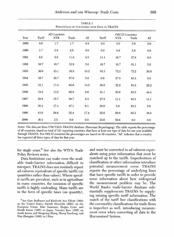
Anderson and van Wincoop Trade Costs
TABLE 1 PERCENTAGEOF COUKTRIESWITH DATAIN TRAINS
All Countries OECD Countries Year Tariff NTB Trade All Tariff NTB Trade All
1989 08 17 17 08 00 00 56 00
2000 364 25 00 00 556 556 00
Notes The data are from UNCTADs TRAINS database (Haveman Repackaging) The table reports the percentage of all countries based on total of 121 reporting countries that have at least one type of data for one year available through TRAINS For OECD countries the percentages are based on 19 countries All indicates that a country has reported all three types of data for that year
for single years9 See also the WTOs Trade and must be converted to ad valorem equiv- Policy Reviews series alents using price information that must be
Data limitations can make even the avail- matched up to the tariffs Imperfections of able trade-barrier information difficult to classification or other information introduce interpret TRAINS does not routinely report potential measurement error TRAINS ad-valorem equivalents of specific tariffs (on reports the percentage of underlying lines quantities rather than values) Where specif- that have specific tariffs in order to provide ic tariffs are prevalent such as in agriculture some information about how widespread in many countries the omission of specific the measurement problem may be The tariffs is highly misleading Many tariffs are World Banks trade-barrier database sub- in the form of specific taxes (on quantity) stantially supplements TRAINS by supply-
ing missing specific tariff information The
See Gaq- Hufbauer and Kimberly Ann Elliott (1994) match of the tariff line classifications with on the United States Patrick Messerlin (2001) on the the commodity classifications for trade flows European Union Yoko Sazana~ni Shujiro Urate and is imperfect as well introducing measure- Hiroki Kawai (1995) on Japan Namdoo Kiln (1996) on South Korea and Shuguang Zhang Zhang Yansheng and ment error when converting all data to the Wan Zhonpn (1998)on China Harmonized System
00
696 Jou~malof Econoinic Literature Vol X L I I (Septeinber 2004)
Nontariff barriers (NTBs) are much more problematic than tariff barriers The World Bank database unfortunately does not pro- vide NTB data A user must use TRAINS or more specialized databases directed at par- ticular NTBs The TRAINS database records the presence or absence of a nontar- iff barrier (NTB) on each six-digit line Manv differing types of nontariff barriers ark recorded in TRAINS (a total of eighteen types) The NTB data requires concordance between the differing NTB tariffs and trade classification svstems at the national level converting to the common HS system
Jon Havemans extensive work with TRAINS has produced a usable NTB data- base Haveman follows what has become a customary grouping of NTBs into hard bar- riers (price and quantity measures) threat measures (antidumping and countervailing duty investigations and measures) and qual- ity measures (standards licensing require- ments etc) A fourth category is embargoes and prohibitions A common use of the NTB data is to construct a measure of the preva- lence of nontariff barriers such as the per- centage of HS lines in a given aggregate that are covered by NTBs Nontariff barrier information in TRAINS is particularly prone to incompleteness and poor-quality problems so analysts seeking to study parti- cular sectors such as the Multi-Fibre Arrangement (MFA) will do better to access specialized databases such as the World Banks MFA data
No information about NTB restrictive-ness is provided in TRAINS since measur- ing the restrictiveness of each type of nontariff barrier requires an economic model In some important cases individual analysts have developed direct measures of
lo See the Ultimate Trade Barrier Catalog at ht m~~veiitorgProtection
Uationd tmff line infornlation is also very problem- atic when analyzing nontariff barriers For example matching up reported trade flows with annual quotas immediateb runs into inconsistencies in reporting conven- tions
the restrictiveness of NTBs based on quota license prices where these are available
Indirect methods of measuring the restric- tiveness of NTBs are important because of the paucity of direct measures One method is to infer the restrictiveness of nontariff bar- riers through the comparison of prices Some important trade lines are well-suited for price comparisons (homogeneous products sold on well-organized exchanges for example) but even here there are important issues with domestic transport and intermediary margins and the location of wholesale markets rela- tive to import points of entry Evidence from price comparisons is discussed in section 4 The restrictiveness of nontariff barriers can also be inferred from trade quantities in the context of a well-specified model of trade flows Inference about nontariff barriers from trade flows is discussed in section 3 Alan Deardorff and Robert Stern (1998) and Sam Laird and Alexander Yeats (1990) pro- vide other detailed discussions of inference about the restrictiveness of NTBs
Aggregation is an important problem in the use and analysis of trade barriers Tariffs and NTBs comprise some 10000 lines with large variation across the lines The national customs authorities are the primary sources of trade restrictions and their classification systems do not match up internationally or even intranationally as between trade flows on the one hand and tariff and nontariff- barrier classes on the other hand Matching up the tariff nontariff and trade-flow data requires aggregation guided by concor-dances that are imperfect and necessarily generate measurement error Moreover for many purposes of analysis the comprehen- sion of the analyst is overwhelmed by detail and further aggregation is desirable Atheoretic indices such as arithmetic (equal- ly weighted) and trade-weighted average tar-
iffs are commonly used while production-weighted averages sometimes replace them for nontariff barriers the
indicator is aggregated into a nontar-iff barrier coverage ratio the arithmetic or
697 Anderson and van Wincoop Trade Costs
trade-weighted percentage of component sectors with nontariff barriers
Ideal aggregation is proposed by James Anderson and Peter Neary (1996 2003) based on the idea of a uniform tariff equiva- lent of differentiated tariffs and NTBs Theoretically consistent aggregation depends on the purpose of the analysis so the analyst must specify tariff equivalence with reference to an objective that makes sense for the task at hand Anderson and Neary develop and apply indices for the small-country case that are equivalent in terms of welfare and in terms of distorted aggregate trade volume12 and show that atheoretic aggregation can significantly bias the measurement of trade restrictiveness13 The theme of appropriate aggregation in the different setting of many countries in gener- al equilibrium plays a prominent role in our discussion of indirect measurement of trade costs so we defer a full treatment to that section Ideal aggregation is informationally demanding so for that reason and because of their familiarity and availability in the work of others we report the standard trade- weighted and arithmetic averages of tariffs and of NTB coverage ratios below
212 Evidence on Policy Barriers
Tariffs Trade-weighted and arithmetic average tariffs are reported in table 2 for fifty
ee also Anderson (1998)for equivalence in terms of sector-specific factor income and its relationship to the com~nonly reported effective rate of protection
l3Anderson and Neaq (2003)report results using a volu~ne equivalent uniform tariff- replacement of the dif- ferentiated tariff structure with a uniform tariff such that the general equilibrium aggregate value of trade in tiistort- eti products (in terms of external prices) is held constant The ideal index is usually larger than the trade-weighted average-an arithmetic average across countries in the study ields approximately 11percent for the trade weight- ed average anti 12 percent for the uniform volume equiv- alent while the US nu~nbers in 1990 are 4 percent and 48 percent respectively For purposes of co~nparison between the initial tariffs and free trade the two indexes are quite highly correlated For a s~naller set of evaluations of year-on-year changes in contrast Anderson anti Neal show that the ideal and trade-weighted average indexes are uncorrelatect
countries for 1999 based on TRAINS data14 The relatively small number of coun- tries reflects reporting difficulties typical of TRAINS some earlier years contain data for more countries The reported numbers aggregate the thousands of individual tariff lines in the underlying data The table con- firms that tariffs are low among most devel- oped countries (under 5 percent) while developing countries continue to have high- er tariff barriers (mostly over 10 percent) Dispersion across countries is wide Hong Kong and Switzerland have 0 percent tariffs the United States has a 19 percent simple average and at the high end India has 301 percent and Bangladesh 227 percent
The variation of tariffs across goods is quite large in all countries typically only a few are large Intuition suggests that the variation of tariffs adds to the welfare cost Marginal deadweight loss is proportional to the tariff hence the cumulated dead weight loss triangle varies with the square of the tar- iff Coefficients of variation (the ratio of the standard deviation to the mean) of tariffs either arithmetic or trade-weighted thus sometimes supplement averages Anderson and Neary (2003) report trade-weighted coefficients of variation of tariffs for 25 coun-tries around the year 1990 ranging from 014 to 167 many being clustered around one Thev show that a proper analysis quali- fies the simple intuition considerably with welfare cost increasing in an appropriately weighted coefficient of variation
Bilateral variation of tariffs can also be large Preferential trade is mainly responsible since insiders face a zero tariff while outsiders face the MFN tariff but aggregation over goods induces further bilateral variation due to differing composition of trade across part- ners James Harrigan (1993) reports bilateral production-weighted average tariffs in 28 product categories for OECD countries for
dculations were based on TRAINS annual data- bases purchased by Boston College without the front- e d software and assembled into panel data
TABLE 2 SILIPLE TARIFFAKD TRADE-VEIGHTED A V E R A G E S - ~ ~ ~ ~
County Simple T V Average Average
Argentina 148 113 Australia 45 41 Bahamas 07 08 Bahrain 78 -Bangladesh 227 218 Barbados 192 203 Belize 197 149 Bhutan 153 -
Boli~ia 97 91 Brazil 155 123 Canada 45 13 (bile 100 100 (oloinbia 122 107 (osta Rica 65 40 (zech Republic 55 -
Ilorninica 185 158 Ecuador 138 111 European Union 34 27 (korgia 106 -
Grenada 189 157 Guyana 207 -
Ilonduras 75 78 Hong Kong 00 00 India 301 -
Illdonesia 112 -
Jiiunaica 188 167
Japan 24 29 Korea 91 59 Mexico 175 66 hlontserrat 180 -
New Zealand 24 30 Nicaragua 105 110 Paraguay 130 61 Peru 134 126 Pllilippilles 97 -
Romania 159 83 Saudi Arabia 122 -
Singapore 00 00 Slovenia 98 114 Soutll Africa 60 44 St Kitts 187 -
St Lucia 187 -
St Uncent 183 -
Suriname 187 -
Switzerland 00 00 Taiwan 101 67 Trinidad 191 170 Ur11gua)i 49 45 USA 29 19 Ve~~ezuela 124 130
Xotcs Tlle data are from UNCTADs TRAINS database (Haveman repackagmg) A -indicates that trade data for 1999 are ullavailable in TRAINS
699 Anderson and van Wincoop Trade Costs
1983 For Canada the reported range of bilateral averages runs from 12 percent to 32 percent and for Japan from 23 percent to 45 percent The United States has more modest differences from 16 percent to 23 percent15
Nontarif Barriers Table 3 reports the prevalence of nontariff barriers for 34 coun- tries in 1999 based on data from TRAINS and Havemans work (rendering it more usable) The smaller number of countries available than for tariffs reflects previously noted limi- tations of TRAINS We report arithmetic and trade-weighted NTB coverage ratios the per- centage of tariff lines subject to NTBs The trade-weighted NTB coverage ratios general- ly exceed the arithmetic average NTB cover- age ratios often considerably so For example on the narrow definition (defined below) the US arithmetic NTB coverage is 15 percent while the trade-weighted NTB coverage is 55 percent This reflects the fact that NTBs tend to fall on important traded goods such as textiles and apparel
Narrow NTB coverage is basically price and quantity control measures and quality control measures while broad coverage is the narrow classification plus threat measures related to antidumping Threats are signifi- cant since Robert Staiger and Frank Wolak (1994) have shown that the threat of antidumping impedes trade considerably (on average for the United States they find a sev- enteen-percent reduction in trade due to an ongoing investigation) Narrow NTBs cover less than 10 percent of trade for the rich countries and modest amounts of trade in most except for Argentina and Brazil Table 3 implies that antidumping is quite common For example based on the TRAINS data the United States in 1999 had 15 percent of tar- iff lines subject to NTB when narrowly defined but 272 percent of tariff lines subject
l5 Harrigans data is available to the public Huiwen Lai and Daniel Trefler (2002) are notable for compiling three- digit bilateral tariffs for fourteen importers and 36 exporters for 1972 1977 1982 1987 and 1992 They emphasize the hard work involved and have not yet made the data public
to NTB when broadly defined These meas- ures do not include withdrawn suits which are presumptively restrictive since they facil- itate collusion Table 3 also shows wide vari- ability over countries in the use of NTBs The broad definition with arithmetic averages has South Africa at 113 percent and Argentina at 718 percent
The use of NTBs is concentrated in a few sectors in most economies Table 4 reports sectoral NTB coverage ratios for the United States European Union Japan and Canada for 1999 NTBs are widely used by devel- oped countries in food products (for exam- ple the trade-weighted NTB coverage of agriculture forestry and fishery products is 74 percent for the United States and 24 per- cent for the European Union) textilesappar- el (71 percent for the United States and 42 percent for the European Union) wood and wood products (39 percent for the United States and 26 percent for the European Union) and in some other areas of manufac- turing The products involved are quite sig- nificant in the trade of developing countries but also somewhat significant in the trade of developed countries with each other
In comparison to tariffs NTBs are con- centrated in a smaller number of sectors and in those sectors they are much more restric- tive Deardorff and Stern (1998) survey most of what limited data is available on quota license prices Table 5 (based on table 36 of Deardorff and Stern 1998) gives estimates of tax equivalents based on annual averages of week1 Hong Kong MFA quota license
(which are themselves averages of
l6Where markets subject to quotas are thick and well- organized and behavior of all agents is competitive quota license prices provide the best evidence of tariff equiva- lents Using license price data even under these assump- tions forces the analyst to face the many dimensions on which the quota is not equivalent to a tariff-daily price quotes exhibit within-year variation with economically sig- nificant patterns (seasonality year-end jumps and drops)- such that no single index of them can generally be equivalent to a tariff Nevertheless average license prices in combination with the substantial rent-retaining tariffs found on most quota-constrained products provide a use-ful measure of the restrictiveness of quotas
TABLE 3 NOY-TARIFFB R R I E R S - ~ ~ ~ ~
NTB ratio Tf7NTB ratio NTB ratio Tf7NTB ratio (narrow) (narrow) (broad) (broad)
Algeria
Argentina
Australia
Ballrain
Bhutan
Bolivia
Brazil
Canada
Chile
Colombia
Czech Republic
Ecuador
European Union
Guatemala
H u n g a ~
Indonesia
Lebanon
Lithuania
Mexico
Morocco
New Zealand
Oman
Paraguay
Peru
Poland
Romania
Saudi Arabia
Slo-enia
South Africa
Taiwan
Tunisia
Uruguay
USA
Venezuela
Xotes Tlle data are from UNCTADs TRAINS database (Haveman repackaging) Tlle narrow cat ego^ includes quantity price quality and ad-ance payment NTBs but does not include threat measures such as antidumping in-estigations and duties The broad categon includes quantity price quality advance payment and threat measures Tlle ratios are calculated based on six-digit HS categories 4 - indicates that trade data for 1999 are not available
Anderson and van Wincoop Trade Costs
TABLE 4 NTH COVERAGE RATIOSBY SECTOR-^^^^
United States 1999 EU-12 1999 Japan 1996 Canada 1999
Narrow Broad Narrow Broad Narrow Broad Narrow Broad
NTB-ratio NTB-ratio NTB-ratio KTB-ratio KTB-ratio KTB-ratio NTB-ratio NTB-ratio
ISIC Description 1 Agric Forestry Fish 011 052 719 743 001 001 229 241 153 227 897 962 028 022 878 938
2 Mining Quarcng 000 000 018 099 001 055 001 055 028 008 193 706 000 000 027 014
21 Coal Mining 000 000 000 000 004 000 004 000 000 000 667 1000 000 000 000 000
22 Crude Petroleum 000 000 250 105 004 067 004 067 000 000 1000 1000 000 000 375 019
23 Metal Ore Mining 000 000 000 000 000 000 000 000 087 000 087 000 000 000 000 000
29 Other Mining 000 000 000 000 001 038 001 038 014 129 120 184 000 000 000 000
3 Manufacturing 015 047 245 423 007 042 083 107 044 102 322 366 171 044 261 196
31 Food Bev Tobacco 072 120 644 809 004 011 489 474 185 329 925 893 185 348 456 453 32 Textiles Apparel 000 002 509 708 030 255 102 420 022 050 163 120 762 681 816 784
33 Wood Toad Prod 000 000 459 389 000 007 197 263 000 000 098 025 016 015 262 252
34 Paper Paper Prod 000 000 053 023 000 000 000 000 000 000 133 036 000 000 000 000
35 Chem Petrol Prod 036 149 114 322 003 011 032 033 048 169 635 750 013 007 047 073
36 Kon-Metal Min Prod 000 006 014 029 000 016 000 043 000 000 073 160 000 000 000 000
37 Basic Metal Ind 003 044 006 044 002 010 012 016 051 086 375 139 000 000 381 362
38 Fab Metal Prod 002 039 166 450 000 010 005 012 032 057 095 266 000 000 048 179 39 Other Manuf 000 002 122 199 000 017 238 222 000 000 134 112 000 000 073 012
Total All Products 015 055 272 389 008 041 095 106 055 098 369 442 151 039 307 198
Notes S indicates simple and TI1 indicates trade-weighted Data are from UNCTADs TRAINS database (Haveman repackaging) The Narrow category includes quantity price quality and advance payment NTBs but does not include threat measures such as antidumping investigations and duties The Broad category includes quantity price quality advance payment and threat measures The ratios are calculated for two-digit ISIC categories based on the six-digit HS classifications used by TRAINS using HS to ISIC concordances published by the World Bank
transactions within the week) for textiles and the license prices to form the full tax equiv- apparel subject to quota behveen controlled alent The table shows fairly high tax equiva- exporters and the United States in 1991 and lents especially in the largest trade 1993 The license prices imputed for other categories (23 percent for products of broad- suppliers depend on arbitrage assumptions woven fabric mills 33 percent for apparel and especially on relative labor productivity made from purchased material) There is assumptions which may not be met The also high variability of license prices and tax prices are expressed as ad-valorem tax equiv- equivalents across commodities (from 5 per-alents using Hong Kong export prices for the cent to 23 percent for textiles from 5 per-underlying textile and apparel items trade- cent to 33 percent for apparel) Earlier years weighted across suppliers17 We add the reveal higher tax equivalents18 Thus there is US tariffs on the corresponding items to
l8Anderson and Neary (1994) report trade-weighted average tax equivalents across the MFA commodity groups
l7 Because the license prices are for transfer between for a set of exporters to the United States in the mid- holders and users and are effectively subject to penalty for 1980s The Hong Kong average exceeded 19 percent in the holder the implied tariff equivalents are lower bounds each year and ranged to over 30 percent in some years to true measures of restrictiveness this bias direction while tax equivalents (very likely biased upward) for other probably also applies to the intertemporal averaging countries were much larger some over 100 percent
702 Journal of Economic Literature Vol XLIl (September 2004)
TABLE 5 TARIFFEQUIULEXTSOF US hfFA QIoT~s 1991 AND 1993 (PERCENT)
Sector 1991 1993
Rent Rent S TIV Rent + US Tar Eq Tar Eq Tanff Tariff TT7 Tariff Imports
Textiles Broadvo-en fabric mills Karrov fabric mills Yarn mills and textile finishillg Thread mills Floor co-erings Felt and textile goods nec Lace and knit fabric goods Coated fabrics not rubberized Tire cord and fabric Cordage and twine Konvoven fabric
Apparel and fab textile products TVomens hosiery except socks HosieT nnec Appl made from purchased mat] Curtains and draperies House furnishings nec Textile bags Can-as and related products Pleating stitching e m b r o i d e ~ Fabricated textile products nec Luggage TVomens handbags and purses
Xotes S indicates simole and 71indicates trade-weirrhted Rent eaui-alents for US imoorts from H o w 0 D
Kong were estimated on the basis of average weekly Hong Kong quota prices paid by brokers using information from International Business and Economic Research Corporation For countries that do not allocate quota rights in public auctions export prices were estimated from Hong Kong export prices with adjustments for differences in labor costs and productivity Sectors and their correspolldillg SIC classifications are detailed in USITC (1995) Table D-1 Quota tariff equivalents are reproduced from Deardorff and Stem (1998) Table 36 (Source USITC 19931995) Tariff a-erages trade-weighted tariff a-erages and US import percentages are calculated using data from the UNCTAD TRAINS dataset SIC to HS concordances from the US Census Bureau are used
(i) substantial restrictiveness of MFA quotas and Canadian agriculture Details are dis- and (ii) very large differentials in quota pre- cussed in section 4 mia across commodity lines and across Using a variety of methods Messerlin exporters (2001) makes a notably ambitious attempt to
Price comparison measures confirm this assemble tariff equivalents of all trade policy picture of the high and highly concentrated barriers for the European Union He com- nature of NTBs with data from the agricul- bines the NTB tariff equivalents with the tural sector European and Japanese agricul- MFN tariffs For 1999 the tariff equivalent of ture is even more highly protected than US policy barriers were 5 percent for cereals
703 Anderson and van Wincoop Trade Costs
648 percent for meat 1003 percent for dairy and 125 percent for sugar In mining the tar- iff equivalent was 713 percent The com-bined arithmetic average protection rate was 317 percent in agriculture 221 percent in textiles 306 percent in apparel and much less in other industrial goods The combined arithmetic average protection rate in industri- al goods was 77 percent We use 77 percent for our representative trade policy cost
22 Transport Costs
Direct transport costs include freight charges and insurance which is customarily added to the freight charge Indirect trans- port user costs include holding cost for the goods in transit inventory cost due to buffering the variability of delivery dates preparation costs associated with shipment size (full container load vs partial loads) and the like Indirect costs must be inferred
221 Measurement Problems and Limitations
There are three main sources of data for transport costs The most direct is industry or shipping firm information Nuno Limao and Anthony Venables (2001) obtain quotes from shipping firms for a standard container shipped from Baltimore to various destina- tions David Hummels (2001a) obtains indices of ocean shipping and air freight rates from trade journals which presumably are averages of such quotes Direct methods are best but not always feasible due to data limitations and the very large size of the resulting datasets
Alternatively there are two sources of information on average transport costs National customs data in some cases allow fine detail For example the US Census provides data on US imports at the ten-digit Harmonized System level by exporter coun- try mode of transport and entry port by weight (where available) and valued at f0b and cif bases Dividing the former value into the latter yields an ad-valorem estimate of bilateral transport cost Hummels (2001a)
makes use of this source for the United States and several other countries The most widely available (many countries and years are covered) but least satisfactory average ad valorem transport costs are the aggregate bilateral cif1fob ratios produced by the IMF from matching export data (re orted f0b) to import data (reported cif)J9 The IMF uses the UNs COMTRADE database supplemented in some cases with national data sources Hummels (2001a) points out that a high proportion of observations are imputed this and the compositional shifts in aggregate trade flows which occur over time lead him to conclude that quality problems should disqualify these data from use as a measure of transportation costs in even semi-careful studies20
222 Evidence on Transport Costs
Hummels (2001a) shows the wide disper- sion in freight rates over commodities and across countries in 1994 The all-commodi- ties trade-weighted average transport cost from national customs data ranges from 38 percent of the f0b price for the United States to 133 percent for Paraguay The all- commodities arithmetic average ranges from 73 percent for Uruguay to 175 percent for Brazil The US average is 107 percent Across commodities for the United States the range of trade-weighted averages is from less than 1 percent (for transport equip- ment) to 27 percent for crude fertilizer The arithmetic averages range from 57 percent for machinery and transport equipment to 157percent for mineral fuels
Hummels (1999) considers variation over time The overall trade-weighted average transport cost for the United States declined over the last thirty years from 6 percent to 4
l9 See the Direction of Trade Statzstics and the li~tenlational Financial Statistics
Nevertheless because of then avallabihty and the difficulty of obtaining better estimates for a w d e range of countries and years apparently careful work such as Harrigan (1993) and Scott Baier and Jeffrey Bergstrand (2001)uses the I M F data
704 Journal of Economic Literature Vol XLlI (September 2004)
percent Composition problems are acute because world trade in high-value-to-weight manufactures has grown much faster than trade in low-value-to-weight primary prod- ucts Hummels shows that air freight cost has fallen dramatically while ocean shipping cost has risen (along with the shift to con- tainerization which improves the quality of the shipping senice) He also documents the vide dispersion in the rate of change of air-freight rates across country pairs over the past forty years
Notice that alongside tariffs and NTBs transport costs look to be comparable in average magnitude and in variability across countries commodities and time Transport costs tend to be higher in bulky agricultural products where protection in OECD coun- tries is also high Policy protection tends to complement natural protection amplifying the variability of total trade costs
Limao and enables (2001) emphasize the dependence of trade costs on infrastructure They gather price quotes for shipment of a standardized container from Baltimore to various points in the world Infrastructure is measured as an average of the density of the road network the paved road network the rail network and the number of telephone main lines per person A deterioration of infrastructure from the median to the 75th percentile of destinations raises transport costs by 12 percent The median landlocked country has transport costs that are 55 per- cent higher than the median coastal econo- my21 The infrastructure variables also have explanator) power in predicting trade vol- ume Inescapably understanding trade costs and their role in determining international trade volumes must incorporate the internal geography of countries and the associated interior trade costs
As for indirect costs I-Iummels (2001b) imputes a willingness-to-pay for saved time
21 Limao and enables also report similar results using the cif1fob ratios of the IILIF
Each day in travel is on average worth 08 percent of the value of manufactured goods equivalent to a 16-percent ad-val- orem tariff for the average-length ocean shipment Shippers switch from ocean to air in his mode choice model when the full (shipping plus time) cost of ocean exceeds that for air22 The use of averages here masks a lot of variation in the estimated value of time across two-digit manufactur- ing sectors and is subject to upward aggre- gation bias due to larger growth in trade where savings are greatest due to the sub- stitution effect Infrastructure is likely to have a considerable effect on the time dosts of trade
In 1998 half of US shipments was by air and half by boat23 Assigning one day to shipment by air anywhere in the world as Hummels does and using the twenty-day average for ocean shipping leads to an average 9-percent tax equivalent of time costs Hummels argues that faster transport (shifting from shipping to air and faster ships) has reduced the tax equivalent of time costs for the United States from 32 percent to 9 percent over the period 1950-9824
We combine percent time costs and 107 percent US average direct transport costs for our representative full transport cost of 21 percent (1107109-1)
Linking port of entry for US imports with the trav- el time to the exporter (a county-average of times to the exporters ports) he creates a matrix of ocean shipping times Air freight is assumed to take one day for points anywhere in the world
This ignores trucking and rail modes which are important to trade with Canada and Mexico the two lar est trade partners of the United States
The calculation is based on observing that US imports excluding Canada and Mexico had 0-percent air shiprnent in 1950 and 50-percent air shipment in 1998 The average ocean shiprnent time was halved from forty days to twent) days over the same time The net effect is a sa~ingof 295 days equal to forty days for 1950 minus 105 days for 1998 The latter is equal to 5 times hvent) days for ocean shipping plus 5 times one day for air freight For manufacturing at 08 per cent ad valorem per day for the value of time in shipping the sa~ing of 295 days is worth a fall from 32 percent to 9 percent ad valorern
Anderson and van Wincoop Trade Costs
TABLE 6 DISTRIBUTIONMARGINSFOR HOUSEHOLDCONSUMPTIONAND CAPITALGOODS
Select Aus Bel Can Ger Ita Jap Net UK US Product Categories 95 90 90 93 92 95 90 90 92
Rice 1239 1237 1867 1423 1549 1335 1434 1511 1435
Fresh frozen beef 1485 1626 1544 1423 1605 1681 1640 1390 1534
Beer 1185 1435 1213 1423 1240 1710 1373 2210 1863
Cigarettes 1191 1133 1505 1423 1240 1398 1230 1129 1582
Ladies clothing 1858 1845 1826 2039 1562 2295 1855 2005 2159
Refrigerators freezers 1236 1586 1744 1826 1783 1638 1661 2080 1682
Passenger vehicles 1585 1198 1227 1374 1457 1760 1247 1216 1203
Books 1882 1452 1294 2039 1778 1665 1680 1625 1751
Office data proc mach 1715 1072 1035 1153 1603 1389 1217 1040 1228
Electronic equip etc 1715 1080 1198 1160 1576 1432 1224 1080 1139
Simple Average (125 categories) 1574 1420 1571 1535 1577 1703 1502 1562 1681
Notes The table is reproduced from Bradford and Lawrence Paying the Price The Cost of Fragmented International Markets Institute of International Economics forthcoming (2003)Margins represent the ratio of purchaser price to producer price Margms data on capital goods are not available for the Netherlands so an average of the four European countries margins is used
23 Wholesale and Retail Distribution Costs show that their input-output estimates of US distribution costs are roughly consis-
Wholesale and retail distribution costs tent with survey data from the US enter retail prices in each country Since Department of Agriculture for agricultural wholesale and retail costs vary widely by goods and from the 1992 Census of country this would appear to affect Wholesale and Retail Trade For other G-7 exporters decisions Local trade costs apply countries they report distribution costs in to both imported and domestic goods how- the range of 35-50 percent ever so relative prices to buyers dont Scott Bradford and Robert Lawrence change and neither does the pattern of (2003) use the same input-output sources to trade Section 3 gives a formal argument measure distribution costs for the United Section 4 discusses the effect of distribution States and eight other industrialized coun- margins on inference about international tries but instead divide by the producer trade costs from retail prices price consistent with the approach in this
Ariel Burstein Joao Neves and Sergio survey of reporting trade barriers in terms of Rebelo (2003) construct domestic distribu- ad valorem tax equivalents Table 6 reports tion costs from national input-output data distribution costs for selected tradable for tradable consumption goods (which household consumption goods and an arith- correspond most closely to the goods for metic average for 125 goods The averages which narrowly defined trade costs are rel- range over countries from 42 percent in evant) They report a weighted average of Belgium to 70 percent in Japan Average 419 percent for the United States in 1992 US distribution costs are 68 percent of pro- as a fraction of the retail price They also ducer prices The range of distribution costs
706 Journal of Economic Literature Vol X L I I (September 2004)
is much larger across goods than across countries for example running from 14 per- cent on electronic equipment to 216 percent on ladies clothing in the United We take 55 percent as our representative domestic distribution cost close to the trad- able consumption goods average of OECD countries
3 Inference of Trade Costs from Trade F1ous
Trade costs can be inferred from an eco- nomic model linking trade flows to observ- able variables and unobservable trade costs Inference has mainly used the gravity
The economic theor) of gravity is developed here extensively revealing new properties that clarify procedures for good empirical work reporting results and doing sensible comparative statics Our develop- ment embeds gravity within the classic con- cerns of trade economists with the equilibrium allocation of production and expenditure within nations
A variety of ad hoc trade cost functions have been used to relate the unobservable cost to observable variables Plausibly cost falls with common language and customs better information better enforcement and so forth Many implementations impose restrictions that seem implausible Some proxies may not be exogenous such as membership in a currency union or regional trade agreement their effects will not be uniform functional form is often too simple and so forth Further economic theory is needed to identify the underlying structure of trade costs
j Iye sshould warn that some of these distribution cost estimates include rents in the form of lnonopolistic markups rather than actual costs incurred by the local dis- tribution sector Although it n~ould be desirable to take out these rents no data are available to do so 4 subset of the gravity literature uses it to discrimi- nate among theories of the determinants of trade It is not very well-suited for this purpose since many trade models ill lead to gra~ity (Deardorff 1998)
31 Traditional Gravity
Most estimated gravity equations take the form
where xg is the log of exports from i toj y and yJ are the log of GDP of the exporter and importer and zy (m=l M) is a set of observables to which bilateral trade barri- ers are related The disturbance term is E
A large recent literature developed estimat- ing this type of gravity equation after a sur- prising finding by McCallum (1995) that the US-Canada border has a big impact on trade McCallum estimated a version of (1)for US states and provinces with two z variables bilateral distance and an indica- tor variable that is equal to one if the two regions are located in the same country and equal to zero otherwise He found that trade between provinces is more than twenty times trade between states and provinces after controlling for distance and size The subsequent literature has often added so-called remoteness variables which are intended to capture the average distance of countries or regions from their trading partners
Gravity equations can be derived from a variety of different theories None lead to tra- ditional gravity despite this literatures use of references such as Anderson (1979) and Deardorff (1998) to justify estimation of
32 Theo y-Based Gravity
Gravity-like structure obtains in a wide class of models those where the allocation of trade across countries can be analyzed
See Michael Anderson and Stephen Smith (1999ab) Natalie Chen (2002) Carolyn Evans (2003abc) John Hellivell (1996 1997 1998) Hellin~ell and John McCallum (1995) Hellivell and Genevieve F7erdier (2001) Russell Hillberry (1998 2002) 1701ker Nitsh (2000) Shang-Jin 17ei (1996) and Holger LVolf (2000ab)
For recent surveys of gravity theory see Harrigan (2002) and Feenstra (20022003)
707 Anderson and can Wincoop Trade Costs
separately from the allocation of production and consumption within countries29 Let Y Elk] be the value of production and expenditure in country i for product class k A product class can be either a final or an intermediate good A model is trade separa- ble if the allocation of ytkk for each coun- Etk try i is separable from the bilateral allocation of trade across countries
Trade separability obtains under the assumption of separable preferences and technology Each product class has a distinct natural aggregator of varieties of goods dis- tinguished by country of origin This assumption allows the two-stage budgeting needed to separate the allocation of expen- diture across product classes from the allo- cation of expenditure within a product class across countries of origin3o What exactly is implied by product differentiation within a product class will differ depending on the product class and its myriad characteristics For inputs of physically standardized prod- ucts (grains petroleum steel plate) differ- entiation may be on terms of delivery or subtle qualities that affect productivity while branded final goods suggest hedonic differ- entiation over varieties of clothing or per- fume Imposing some form of differentiation is unavoidable if empirical trade models are to fit the bilateral trade data as Armington noted long ago
The class of trade separable models yields bilateral trade without having to make any assumptions about what specific model accounts for the observed output structure Y and expenditure allocations
The general equilibrium of trade in a many-country world is enorlnously simplified by this natural assumption
30Explicitly separabiliv restricts the dual cost function c ( p w y )where p is a vector of traded input prices and w is a vector of non-traded primary input prices n~hile y is the level of output The separability restriction is imposed in c(p u- y )=f lg(p) u- y]where g ( p ) is a homogenous of degree one and concave function of p By Shephards Lemma f is the aggregate demand for the traded input class while fg is the demand vector for the individual products A similar structure characterizes the assumption of separability in final demand
~ k ~ lBilateral trade is determined in con-ditional general equilibrium whereby prod- uct markets for each good (each brand) produced in each country clear conditional on the allocations ytkk Etk] Inference about trade costs is based on this conditional gen- eral equilibrium Comparative static analy- sis in contrast requires consideration of the full general equilibrium A change in trade barriers for example will generally affect the allocations Y E]
Two additional restrictions to the class of trade separable models yield gravity These are the aggregator of varieties is identical across countries and CES and ad-valorem tax equivalents of trade costs do not depend on the quantity of trade The CES form imposes homothetic preferences and the homogeneity equivalent for intermediate input demand These assumptions simplify the demand equations and market clearing equations These two restrictions can be relaxed in various useful ways discussed below Our derivation provides much more context to Deardorffs (1998) remark I sus- pect that just about any plausible model of trade would yield something very like the gravity equation
If X is defined as exports from i to j in product class k the CES demand structure implies (under the expositional simplifica- tion of equal weights for each country of origin)
where a is the elasticity of substitution among brands pi is the price charged by i for exports to j and P is the CES price index
Specifically it does not matter what one assumes about production functions technology the degree of competition or specialization patterns The nature of pref- erences and technology that gives rise to the observed expenditure allocations E also does not matter
708 Journal of Econoinic Literature Vol XLII (September 2004)
The assumption that trade costs are pro- portional to trade implies that the price p can be written as pftwhere p f is the sup- ply price received by producers in country k and ti-1 is the ad-valorem tax equivalent of trade costs independent of volume
If supply is monopolistic the supply price is the product of marginal production cost and the markup So long as the markup is invariant over destination^^^ t i contains only trade costs Otherwise the tax equiva- lent must be interpreted to contain markups With competitive supply this issue does not arise Markups arising from monopoly power in the distribution sector itself are a more important issue with interpreting ti-1 as a cost
Imposing the market-clearing conditions
for all i and k yields gravity Solve for the supply prices p from the market-clearing conditions and substitute the result in (2) and (3)This yields the system
where yk is world output in sector k The indices P and flk can be solved as a function
32 LVith Cournot competition the markup is invariant over destinations in symmetric rnonopolistic competition Generally it is equal to l [ l - l ~( l - s ~) ] is the mar- where s ket share of i inj
of trade barriers (t] and the entire set (Y E~] Trade flows therefore also depend on trade barriers and the set ( Y E ~ ) ~ ~
A wide variety of production and expen- diture models may lie behind (EY~In particular some of the Es and 2s may be equal to zero Previous derivations of gravi- ty have usual1 made much more restrictive assumptionsJ
The main insight from the theory is that bilateral trade depends on relathe trade bar- riers The key variables fl and P are out- ward and inward multilateral resistance respectively They summarize the average trade resistance between a country and its trading partners in an ideal aggregation sense which we develop below Basic demand theory suggests that the flow of good i intoj is increased (given ugtl)by high trade costs from other suppliers to j as captured by inward multilateral resistance P But less obviously high resistance to shipments from i to its other markets ca P tured in outward multilateral resistance Hitips more trade back into is market in j Gravity gives these insights an elegant1 sim le form in (5) Y PThe trade cost tVmay include local distri- bution costs in the destination market but those domestic costs do not affect trade flows This rather surprising and important result follows from basic gravity theory Suppose for any goods class k that each destination j has its own domestic margin m If we multiply all
Theoretical gravity equations in Anderson (1979) Jeffrey Bergstrand (198519891990) and Scott Baier and Bergstrand (2001) look far more complicated than (3 with a large number of prices and price indices Anderson and van Lfincoop (2003) show that all these prices can be surnrnarized by just two price indices one for the importer and one for the exporter which are solved as a function of trade barriers and total supply and dernand in each location
34 The first paper to formally derive a grality equation from a general equilibrium model with trade costs is Anderson (1979) who assumes that every country pro- duces a particular variety Bergstrand (1989 1990) and Baier and Bergstrand (2001) derive gravity equations in models with rnonopolistic competition endogenizing vari- ety Anderson and van incoop (2003) assume each coun- try has an endovment of its good
709 Anderson and uan Wincoop Trade Costs
narrowly defined trade barriers tlJ by domes- tic trade costs mkin the destination market it is easily verified from (6)-(7) that the P are multiplied by m the are unchanged and therefore trade flows are also unchanged
The invariance of trade patterns to domes- tic distribution costs that apply to all goods has another important practical implication We can only identify relative costs with the gravity model One way to interpret an inferred system of trade costs ti] is to I ick some region i and normalize t = l Essentially this procedure treats the trade cost of i with itself as a pure local distribu- tion cost and divides all other trade costs by the local distribution cost in region i
As in most gravity papers Anderson and van Wincoop (2003) consider a one-sector economy They show that when consumers have CES preferences with common elas- ticity a among all goods the gravity equa- tion can be written omitting the superscripts k as
where Y and Y are levels of GDP Y is world GDP and 0 is the income share of country i This is a special case of (5) with expenditure equal to output because it is a one-sector economy (E=Y) With symmetry of trade costs (t=t) n=P
A couple of comments are in order about homogeneous goods trade When we let the elasticity of substitution ak in (5)-(7) go to infinity trade converges to that in a homoge- neous goods model However no informa- tion about trade barriers can be inferred As an example consider a two-country model with trade in a homogeneous good k If country 1exports k to country 2 its export is
equal to ~k-Yk Gravity equation ( 5 ) accounting for multilateral resistance indeed converges to this for the two-count17 case as a approaches infinity assuming any non-zero international trade barrier (and normalizing domestic barriers to zero) Since the bilateral trade flow in the condi- tional general equilibrium does not depend on the magnitude of trade barriers nothing can be learned about trade barriers More generally it is difficult to learn much about trade barriers from a gravity equation for sectors where the elasticity of substitution is extremely high The expressions t-hn which trade flows (directly and through mul- tilateral resistance) depend are virtually zero when a is very high as long as the trade bar- rier is positive (tgtl) Conditional on a trade barrier being positive the size of the trade barrier does not matter much to the pattern of trade flows in the conditional general equilibrium hence we cannot learn much about their size
Several authors have derived gravity equa- tions for homogeneous goods trade when trade is an aggregate of a variety of homoge- neous goods Deardorff (1998) derived a gravity equation in the Heckscher Ohlin model with complete specialization This is essentially a differentiated goods model though with each country producing a dif- ferent brand It does not mean much to say that a good is homogeneous when there is only one producer
A real homogeneous goods model with multiple producers of the same homoge-neous good is the Ricardian model of Jonathan Eaton and Samual Kortum (2002) Their model leads to a gravity equation for an aggregate of homogeneous goods It is also a model with trade separability although the rationale is somewhat different Production is Ricardian with the cost of pro- duction in country i in good k given by clz(k) where z(k) is the realization of tech- nology in good k an element in a continuum of goods Productivity is drawn from a Frdchet distribution The distribution has
710 Journal of Economic Literature Vol X L I I (September 2004)
two parameters The first is Twith higher T meaning a higher average realization for country i The second is 8 with a larger value implying lower productivity differ-ences across countries For a particular good users always buy from the cheapest source The price is the production cost times the trade cost t Each good is pro- duced with both labor and a bundle of inter- mediate goods that consists of the same CES index of all final goods as the utility function over final goods
Since there is a continuum of goods and the setup is the same for all goods (same pro- duction function same productivity distribu- tion same trade cost) the fraction that countnj spends on goods from i is equal to the probability for any particular good that j sources from i With the assumed Frdchet distribution this is equal to
The probability of shipment from country i is lowered by the trade cost of getting the good to country j relative to the average trade cost of shipping from all other destina- tions and lowered by a higher cost of labor The same mathematical representation of the allocation of trade arises as with the CES structure of demand for goods differentiated by place of origin This equation is the same as (2) with a=8+1 and pI1- replaced by Tcll-The p is essentially replaced by c which can be solved in the same way from the conditional general equilibrium This gives rise to the same gravity equation as beforel5
It is worth noting that gross output is now larger than net output due to the input of intermediates The output in the gravity equation (8) is gross output Since Eaton and Kortum assume that intermediates are a fraction 1-P of the production cost c with
ji Eaton and Kortum onl) derwe a graltv spec~ficat~on for X X
labor a fraction P gross output is 11P times value added If we interpret Y in (8) as value added the gravity equation must be multiplied by 1IP
33 The Trade Cost Function
The theoretical gravity model allows infer- ence about unobservable trade costs by (i) linking trade costs to observable cost proxies and (ii) making an assumption about error terms which link observable trade flows to theoretically predicted values Here we focus on (i) the next section deals with (ii) For now we will focus on inference about trade barriers from the aggregate gravity equation (8) In a section about aggregation below we will return to the disaggregated gravity equation (5)
Bilateral trade barriers are assumed to be a function of observables z commonly loglinear
W
Normalizing such that z$=1 measures zero trade barriers associated with this variable (z)ril is equal to one plus the tax equivalent of trade barriers associated with variable m The list of observable arguments 2 which have been used in the trade cost function in the literature includes directly measured trade costs distance adjacency preferential trade membership common language and a host of others Gravity theory has used arbi- trary assumptions regarding functional form of the trade cost function the list of vari- ables and regularity conditions
As an illustration of the functional form problem consider distance By far the most common assumption is that t=d Gene Grossman (1998) argues that a more reason- able assumption is that ~=t-l=d since one can think of z as transport costs per dollar of shipments Hummels (2001a) estimates the p in the second specification by using data on ad-valorem freight rates and finds a value of about 03 Limao and Venables (2001) esti- mate the first specification using cif1fob
Anderson and uan Wincoop Trade Costs
data and also find an estimate of p of about 03 Although these numbers are the same they are inconsistent with each other If the Grossman specification is correct with p=03 one would expect a distance elasticity oft of 03ziJ(1+q1) evaluated at some average z which is much less than 03 Highly mislead- ing results for trade barrier estimates arise when the wrong functional form is adopted
Eaton and Kortum (2002) generalize the treatment of distance with a flexible form which can approximate both of the preceding specifications They assume that there are dif- ferent trade barriers for six different distance intervals While implicitly they still assume a particular functional form in the form of a step function this spline approach is likely to be more robust to specification error
Another functional form issue is that the most common setup (11)is multiplicative in the various cost factors Hummels (2001a) argues that an additive specification is more sensible A multi-dimensional generalization of the approach by Eaton and Kortum (2002) may be applied although there is a tradeoff between degrees of freedom and generality of the specification To the extent that theory has something to say about the functional form it is preferable to use this information over econometric solutions that waste degrees of freedom
The second problem is which observables to include Empirical practice can improve with a more theoretical approach to the zs Especially for abstract trade barriers such as information costs it is often unclear what specific variables are meant to capture Even in the absence of a specific theory it is useful to ponder the relationship between trade barriers and observed variables For example common empirical practice uses a language variable that is one if two countries speak the same language and zero otherwise Jacques Melitz (2003) considers ways in which lan- guage differences affect trade and develops several variables that each capture different aspects of communication One such variable is direct communication which depends on
the percentages of people in two countries that can speak the same language Another is the binary variable open-circuit communica- tion which is one if two countries have the same official language or the same language is spoken by at least 20 percent of the popu- lations of both countries The first variable reflects that trade requires direct communi- cation while the second variable is meant to capture an established network of translation Another example is distance It is common to model distance as the Great Circle distance between capitals Where these differ from commercial centers it is sometimes taken to be superior to use distance between com-mercial centers But then what of countries with more than one commercial center of interior i n f r a s t r~c tu re~~
Implausibly strong regularity (common coefficients) conditions are often implicitly imposed on the trade cost function For example the effect of membership in a cus- toms union or a monetary union on trade costs is often assumed to be uniform for all members As for customs unions a uniform external tariff is indeed approximately the trade policy (though NTBs remain inherent- ly discriminatory) while free trade agree- ments continue to have different national external tariffs and thus different effects As for monetary unions the effect of switching from national to common currencies is like- ly to be quite different depending on the national currency Similar objections can be raised to a number of the other commonly used proxies z y such as common language or adjacency dummies NTBs present an acute form of this problem The effect on trade barriers of NTBs in a country i will general- ly vary across trading partners j goods k and time t Regression residuals reflect the NTBs but also random error To identify the tariff equivalent of NTBs Harrigan (1993)
36 Some investigators (eg Bergstrand) measure bilat- eral distance between ports supplemented by twice the land distance between ports and commercial centers reflecting the rough difference in cost between water and land shipment
712 Journal of Economic Literature Vol XLIl (Septeinber 2004)
assumes not very plausibly that the import- ing countrys NTB has the same trade dis- placement effect for each exporter i that it buys good k from Trefler (1993) assumes even less plausibly that US NTBs have the same trade-reducing effect for all goods k that it imports from the rest of the world 37
We sympathize with efforts to identify trade costs with simple forms of (11) Our criticism of the ad hoc functional form and the regularity assumptions aims to stimulate improvement in estimation and useful com- parative statics Unpacking the reduced form to its plausible structural elements will aid both
34 Estimation of Trade Barriers
Given the trade cost function the loga- rithmic form of the empirical gravity equa- tion becomes (dropping the constant term)
where x=ln(X ) y=ln(Y) and Am=(l -o)~ r and y are oiservables and 5 is the error term
The theoretical gravity equation can be estimated in three different ways38 Anderson and van Wincoop (2003) estimate the structural equation with nonlinear least squares after solving for the multilateral resistance indices as a function of the observables 2 (bilateral distances and a dummy variable for international borders) and the parameters A Another approach
37 Both authors implicitly impose a further regularit) condition NTB coverage ratios for each good are the explanatory variable so all changes in this ratio are assumed to be equally important
38 A potential fourth method is to infer all bilateral trade barriers for a group of countries or regions from the residuals of the bilateral trade flows from the prediction of the frictionless gravit) model The information in this measure would be drowned in random error however there is an unboundedly large confidence in tend about the point estimates because all degrees of freedom are used up
which also gives an unbiased estimate of the parameters A is to replace the inward and outward multilateral resistance indices and production variables y-(1-o)lnP and y-( 1-o)ln(Il) with inward and outward region-specific dummies With symmetry a single set of region-specific dummies suffice This approach is adopted by Anderson and van Wincoop (2003) Eaton and Kortum (2002) Asier Minondo (2002) Andrew Rose and van Wincoop (2002) and Hummels (2001a) Keith Head and Thierry Mayer (2001) and Head and John Ries (2001) fol- low an estimation approach that is identical to replacing multilateral resistance variables with country dummies in the case where internal trade data X exist for all regions or countries Assuming that z=zJ it follows from (12) that
The parameters Ak can then be estimated through a linear regression
A third method is to use data for the price indices and estimate with OLS This requires data on price levels for a cross-sec-tion regression or changes in price indices when there are at least two years of data The latter is the approach taken by Bergstrand (1985 1989 1990) Baier and Bergstrand (2001) and Head and Mayer (2000) As discussed in Baier and Berstrand (2001) it is often hard or impossible to measure the theoretical price indices in the data Price indices such as the consumer price index also include nontradables and are affected by local taxes and subsidies Nominal rigidities also affect observed prices and have a big impact on relative prices when combined with nominal exchange rate fluctuations Anderson and van Wincoop (2003) also argue that certain trade barriers such as a home bias in prefer- ences do not show up in prices Similarly Deardorff and Stern (1998) explain why cer- tain NTBs affect trade but not prices
713 Anderson and van Wincoop Trade Costs
Feenstra (2003) sums it up by writing that the myriad of costs involved in making transactions across the border are probably not reflected in aggregate price indices This does not mean that prices of individual tradable goods are entirely uninformative about trade costs We turn to that topic in section 4
The tax equivalent of trade barriers between i andj associated with variable m is estimated as
This shows that we need an estimate of CJ
in order to obtain an estimate of trade barri- ers Assumptions about o can make quite a difference For example the estimated tax equivalent is approximately nine times larg- er when using o=2 instead of o=10
Gravity can only measure trade barriers relative to some benchmark as noted above The literature tends to compare trade barri- ers between countries to barriers within countries or barriers between regions to barriers within regions This is problematic since different countries or regions have dif- ferent barriers for internal trade The results will also depend on the measure of barriers within a region or country such as the treatment of distance within a country or region This is essentially an aggregation problem since a country or region is itself an aggregate Head and Mayer (2001) Helliwell and Verdier (2001) and Russell Hillberry and David Hummels (2002a) show that the different measures of internal distance can make a big difference for the results
The error term in the empirical gravity literature is usually taken to reflect meas-urement error Trade flow data are notori- ously rife with measurement error39 which is taken to justify a normally distributed additive error term which is orthogonal to
39 For example mirror-image trade flow data do not match
the regressors More careful consideration of measurement error is likely to be produc- tive Some recent implementations recog- nize the panel nature of the data in constructing standard errors (all bilateral observations from i or into j ma have com- mon disturbance elements)lJ Improved econometric techniques based on careful consideration of the error structure are like- ly to pay off Recent literature on spatial econometrics (eg H H Kelejian and Ingmar Prucha 1999) may be helpful
The error term may also reflect unobserv- able variables in the trade cost function (11) If the trade cost t is multiplied by eEy there is again an additive error term in the empirical gravity equation (12) In this case the structural estimation technique dis-cussed above would have to be modified since the multilateral resistance variables also depend on these error terms But the second estimation technique replacing the multilateral resistance variables with region or country-specific dummies is still appro- priate Eaton and Kortum (2002) introduce the error term in this way and adopt the sec- ond estimation method
Non-orthogonality of the error term has two sources omitted variables and endo- geneity If the error term reflects omitted trade frictions which are correlated with the included Z variables it causes estimation bias Endogeneity problems arise in several ways Concerned that trade can affect out- put many papers use instrumental variables for output Y and Y The most common instruments are population or factor endow- ments l1With coefficients on the ys con-strained to one the natural implementation is to make the dependent variable size-adjusted trade x-y-y as Anderson and van Wincoop (2003) do Endogeneity issues also arise when the proxies for trade costs are
40 See for example James Anderson and Douglas Marcou~ller(2002)
41 See for example Exans (2003a)Harngan (19931and el (1996)
714 J o ~ ~ r n a lof Economic Literature Vol XLII (September 2004)
endogenous Examples are membership in currency unions or free trade agreements Section 372 below discusses how the liter- ature has addressed endogeneity in these specific cases
35 Estimation Bias with Traditional Grauity Equations
The traditional gravity equation (1)omits the multilateral resistance terms of the theo- retically consistent model (12) In the absence of multilateral resistance the two equations are the same with amp=Am In that case ( Z ~ ) P ( ~ ~ ~ is an estimate of one plus the tax equivalent of trade barriers associated with this variable This interpretation of the results from estimating (1)is generally incor- rect because the z are correlated with the multilateral resistance indices which are themselves a function of trade barriers
In order to better illustrate this point con- sider the following simplified environment There are two countries the United States and Canada with respectively N states and M provinces The only trade barrier is a bor- der barrier between states and provinces (ignore distance and other factors generating trade barriers) In that case t=bsg where b is one plus the tariff equivalent of trade barri- ers associated with the border and 6 is equal to zero when hvo regions are located in the same country and equal to one other- wise The gravity equation is then (dropping the constant term)
If we ignore multilateral resistance the estimate of (l-o)ln(b) is equal to the aver- age within-country size adjusted trade minus the average cross-country size-adjusted trade When there are N observa- tions of trade within the United States (between states) and M observations of trade within Canada (between provinces) it is easy to check that the estimate of (l-o)ln(b) when ignoring the multilateral
resistance terms is equal to (l-o)ln(b) plus the bias
M - N(1-a)- (InP - InPC)
N +hl (16)
where P and PC are the multilateral resist- ance indices for respectively US states and Canadian provinces PgtP because Canada is smaller and provinces face border barriers with trade to all of the United States The result is that for agtl the estimate of (l-a)ln(b) is biased upwards as long as MgtN This result is intuitive If for example the only within-country trade in the sample is between provinces the average size-adjusted within-country trade is very large The reason is that relative trade barriers within Canada are lower than within the United States due to larger multilateral resistance so that size- adjusted trade is larger between provinces than between states This point way empha- sized by Anderson and van Wincoop (2003)
The example above emphasizes size but estimation bias holds more Consider the role of distance When t=db
general11 the gravity equation becomes (4) with the term (l-o)pln(d) added There are two types of bias when attempting to estimate the border barrier b in a traditional gravity equation that omits multilateral resistance First the distance elasticity (l-o)p is gener- ally incorrectly estimated since bilateral dis- tance is correlated with the multilateral distance terms that are left in the error term Second even when (l-o)p is estimated cor- rectly we still obtain the same bias as in (16) The bias results as long as the multilateral resistance terms P C and P are different Differences arise due to size but also due to geography For example Canadian provinces are located on the North American periphery As a result their dis- tances from main trading partners tend to be relatively large so that PgtP A McCallum type gravity equation with N=O would then imply a positive US-Canada border barrier even when none existed If the geographic size of Canada were much
715 Anderson and van Wincoop Trade Costs
smaller so that trading distances between provinces are much smaller PC would be smaller and the bias from estimating the border barrier b with McCallums equation (N=O) would be smaller Serge Coulombe (2002) emphasizes the role of these topolog- ical issues related to the special structure of the regions42
36 The Elasticity of Substitution
Estimates of trade costs from trade flows are very sensitive to assumptions about the elasticity of substitution a so a look at the evidence is worthwhile Although many papers have estimated this elasticity from bilateral trade flow models only a few have used theory-based gravity
One way to obtain an estimate of a is to use information from directly observed trade barriers Harrigan (1993) Hummels (2001a) Head and Ries (2001) and Baier and Bergstrand (2001) all combine estimation of theoretical gravity equations with informa- tion about tariffs andlor transport costs
Hummels (2001a) assumes
where tar is the tariff rate andamp is a freight factor equal to one plus the tax equivalent of freight costs The gravity equation then becomes (dropping the constant term)
The elasticity of substitution can now be estimated through the coefficient on the log
42 t7l1ile we have focused the discussion on US-Canada estimation bias when estimating the traditional grawity equation of course holds quite generally Some authors have estimated both equations to allow for easy comparison For example Rose and van incoop (2001) find that the estimated trade barriers associated with the use of different currencies are much lower wvllen estimating the theoretical grawity equation Minondo (2001) finds that the estimate of border barriers for European trade is much lower wvllen estimating the theoretical grawity equation
of directly observed trade costs Hummels estimates (18) for 1992 data on sectoral imports of six countries from a large number of other countries Multilateral resistance terms are replaced by country dummies for each sector The estimated elasticity r i~es from 479 for one-digit SITC data to 826 for four-digit SITC data
Head and Ries (2001) adopt a similar method They consider two countries the United States and Canada and assume that the only trade barrier is a border-related bar- rier which varies across three-digit industry data from 1990 to 1995 They estinlate (a-l)ln(b) with b equal to one plus the tar- iff equivalent of the border barrier in indus- try i at time t43 They then decompose the border barrier into tariff and nontariff com- ponents b=(l+tar)(l+NTB) It is assumed that ln(l+NTB1)=amp+~ where K is a time dummy and E is a zero mean random distur- bance By regressing the estimate of (1-a)b on a time dummy and ln(l+tar) they obtain an estimate of both a and average nontariff barriers across industries This approach is similar to that in Hummels (2001a) in that it uses evidence on observed trade barriers to tie down the elasticity Head and Ries obtain an estimate of a of 114 when assuming that NTB is the same for all industries and 79 when allowing for industry fixed effects
Baier and Bergstrand (2001) estimate a theoretical gravity equation where tariffs and transport costs are the only trade barriers They use aggregate trade data for OECD countries and focus on changes in trade flows from the period 1958-60 to the period 1986-88 Their point estimate of a is 64
Harrigan (1993) implicitly models the impact on full trade costs of directly observed trade costs asJ(l+tar) and finds significantl different coefficients on lnf1 and In (1+tar) in the gravity regressions His restricted regres- sions report most elasticity point estimates for
43 In this setup the estimate is obtained as a simple ana- lytical function of the shares that both countries spend on their ow1n goods
1716 Journal of Economic Litel rature Vol XLlI (Septeinber 2004)
28 sectors in the range from five to ten with four above and one below
An entirely different way to estimate a is to simply estimate demand equations direct- ly using data on prices But in general one estimates some combination of demand and supply relationships the classic simultaneity problem Feenstra (1994) is nonetheless able to obtain an estimate of the demand elasticity by using the fact that the second moments of demand and supply changes (their variances and covariance) have a lin- ear relationship that depends on demand and supply elasticities By assuming that supply elasticities are the same for all coun- tries a cross-section of the second moments allows for estimation of the elasticities This estimation method therefore requires panel data and is applied bv Feenstra to US imports from 1967 to 1987 from various countries for six manufactured products The products are highly disaggregated finer than eight-digit SITC The estimated elas- ticities range from three for typewriters to 84 for Treceivers
Eaton and Kortum (2002) adopt vet another entirelv different approach to obampn an estimate of aFrom (8) it follows that
The numerator consists of observables The denominator is approximated as follows Using data on retail price levels for fifty manufactured products in nineteen coun-tries they approximate ln(P)-ln(P) as the arithmetic average of the log-price differen- tials behveen j and i for all 50 goods Using the fact that log-price differentials behveen j and i are bounded above by ln(t)-ln(t) they estimate ln(t)-ln(t) as the maximum of log- price differentials behveen i and j The parameter 8=a-1can then be estimated as the average of the ratio on the right hand side of (19) Thev find 0=828 so that a=928
Overall the literature leads us to conclude that a i s likely to be in the range of five to ten
37 The Size of International Trade Barriers
In this section we report some results for international trade barriers computed as the ratio of total trade barriers relative to domes- tic trade barriers tt We first present sum- mary measures of all international trade barriers and then discuss results which decompose border barriers into several like- ly sources All our calculations are based on point estimates from gravity studies which differ somewhat in their list of trade cost proxies in the data used and in the assump- tions used to construct standard errors
371 Su iiziiza y Measures
Part of the empirical gravity literature reports the tax equivalent of summary meas- ures of trade barriers those associated with distance and the presence of borders Table 7 presents the results of a number of studies The table indicates whether results are based on the traditional gravity equation (1) or the theory-based gravity equation (12) It also indicates whether numbers are based on aggregate trade data or disaggregate (sec- toral) trade data In the latter case table 7 reports the average trade barrier across sec- tors Column four reports the tax equivalent of trade barriers reported by the authors with the corresponding elasticity a in brack- ets In order to make results more compara- ble across papers the final three columns re-compute the trade barriers for elasticities of five eight and ten These are representa- tive of the elasticities estimated in the litera- ture In some cases two numbers are shown with the lower number applyng to countries that share the same language and border
The first three rows report results for total international trade barriers The results are sensitive to the elasticity of substitution For example the US-Canada trade barrier based on the Head and Ries (2001) stud11 ranges from 35 percent for a = l O to 97 Per- cent for a=5 From now on we will focus the discussion on the intermediate value of a=8 In that case the findings by Head and Ries
Anderson and van Wincoop Trade Costs
TABLE 7 TampRIFFEQUIV~LEUT COSTSOF TRADE
method data reported
by authors a = 5
all trade barriers Head and Ries (2001) new disaggr 48 97
US-Canada 1990-1995 (a= 79)
Anderson and van TVincoop (2003) new 91 US-Canada 1993
Eaton and Korturn (2002) new ar 48-63 123-174 19 OECD countries 1990 (u= 928) 750-1500miles apart
national border barriers tVei (1996) trad aggr 5 2676
19 OECD countries 1982-1994 (a=20)
Evans (2003a) trad disaggr 45 45 8 OECD countries 1990 (a=5)
Anderson and van TVincoop (2003) new ar 48 48 US-Canada 1993 (a=5)
Eaton and Korturn (2002) new ar 3245 77-116 19 OECD countries 1990 (a= 928)
language barrier Eaton and Kortum (2002) new ar 6 12
19 OECD countries 1990 (a=928)
Hummels (1999) new disaggr 11 12 160 countries 1994 (u= 63)
currency barrier Rose and van TVincoop (2001) new ar 26 26
143 countries 1980 and 1990 (a=5)
Notes This table reports findings in the gravity literature on the tariff equivalent of a variety of factors that increase trade barriers The second column indicates wvhether estimates are based on the traditional gravity equa- tion -trad- or the theory-based gravity equation -newn The third column indicates wvhether estimation is based on aggregate or disaggregate data The numbers in the fourth column have been reported by the authors for various elasticities of substitution s that are shown in brackets For results based on disaggregated trade data the average trade barrier across sectors is reported (for Hummels (1999)only sectors with statistically significant estimates are used) The numbers in the last three columns re-compute these results for alternative values of a For results based on disaggregate data the trade barriers are first re-computed for each sector and then averaged (with the exception of Head and Ries (2001)who only report average trade barriers across all sectors) When two numbers are reported the lower number applies to countries that share a border and have a comlnon language
(2001) imply an average US-Canada trade barrier for 1993 virtually the same as Head barrier of 47 percent based on average and Ries (2001) This is calculated as the results from 1990 to 1995 Based on trade-weighted average barrier for trade Anderson and van Wincoops (2003) results between states and provinces divided bv the their estimated trade cost parameters with trade-weighted average barrier for trade a=8implv a 46-percent US-Canada trade within the United States and Canada Eaton
718 Journal of Economic Litel pature Vol XLIl (September 2004)
and Kortum (2002) report results for nine- teen OECD countries for 1990 For coun- tries that are 750-1500 miles apart the trade barrier is 58-78 percent The lower 58 per- cent number which applies to countries that share a border and language is not much larger than the estimates of the US-Canada barrier Summarizing international trade barriers are in the range of 40-80 percent for a representative elasticity estimate
Edward Balistreri and Russell Hillberry (2002) argue that trade barrier estimates from these types of studies are implausibly large Based on parameter estimates in Anderson and van Wincoop (2003) they report on trade barriers for Alberta and Alabama relative to the barrier of trade with- in Maryland which has the lowest trade bar- rier As an illustration thev report a trade barrier behveen Alabama and Quebec of 1684 percent for a = 3 and 322 percent for a=5 These numbers are much larger than the 46 percent US-Canada trade barrier reported above There are several reasons for this discrepancy First elasticities of three and five are low relative to estimates in the literature reported above If we set a=8 the Alabama-Quebec barrier drops to 133 percent relative to the Maryland barrier Second Balistreri and Hillberry report trade barriers relative to Maryland instead of rela- tive to average domestic trade barriers as in the papers discussed above Thev therefore also capture trade barriers withinthe United States which are known to be very large based on the direct evidence on distribution costs reported in section 2 The trade barri- er for Alabama-Quebec trade relative to within-US trade is 61 percent The latter is still a bit above the 46-percent US-Canada barrier reported above since Alabama and Quebec are farther apart than the average state-province pair
International trade barriers can be decom- posed into barriers associated with national borders and barriers associated with geo- graphic frictions such as distance The next set of rows in table 7 report the magnitude of
international trade barriers associated with borders For a=8 the estimated US-Canada border barrier from Anderson and van Vincoop (2003) is 26 percent Vith a total barrier of 46 percent it implies a dis- tance related barrier of 16 percent (116= 1461126) This is not much different than direct estimates of trade costs reported in section 11 the total transport cost estimate for the United States is 21 percent (121= 1107109 with 107-percent freight cost and 9-percent time cost) In our repre- sentative total trade cost calculation we assume all effects of distance are captured in the transport cost number (Hummels reports partial success in testing this hypothesis with his disaggregated data)
Although based on traditional gravitv equations estimates of border barriers in Wei (1996) and Evans (2003a) are not too far off respectively 14-38 percent and 30 per- cent Both applv to OECD countries The results from Eaton and Kortum (2002) are a bit higher 39-55 percent Eaton and Kortum do not actually report barriers associated with national borders The 39-55 percent barrier applies to trade costs of countries 0-375 miles apart relative to domestic trade costs Since even for those countries the average distance is larger than within coun- tries it overstates a bit the barrier associated with borders But our own calculations based on estimates from Anderson and van Wincoop (2003) indicate that this overstate- ment is only about 6 percent Summarizing barriers associated with national borders are in the range of 25-50 percent for a represen- tative elasticity estimate44
All the trade costs estimates reported above are based on point estimates Standard errors tend to be quite small though as the empiri- cal fit of gravity equations is general111 very strong For example a 95-percent confidence
44 There is also a small literature that has documented border barriers at the level of states within the United States See f701f (2000ab) Hillberry and Hummels (2002a) and Daniel Millirnet and Thornas Osang (2001)
719 Anderson and van Wincoop Trade Costs
intend of US-Canada border barriers based on Anderson and van Vincoop (2003) is 23 percent-28 percent Standard errors of trade costs associated with distance are even smaller
372 Decomposition of Border Barriers
It is of great interest to better understand what blocks build these border barriers We saw in section 2 that policy barriers in the form of tariffs and NTBs amount to no more than about 8 percent for OECD c~unt r ies ~ suggesting important additional barriers associated with national borders Estimates of five different types of trade frictions are associated with national borders
Language Barriers Table 7 reports esti- mates from Eaton and Kortum (2002) and Hummels (2001a) on language-related barri- ers Thev both follow the common approach of introducing a dummv variable that is one if two countries have B common language and zero otherwise Results from both papers imply a tax equivalent associated with speak- ing different languages of about 7 percent when u=8
Currency Barriers The use of different currencies may pose a barrier to trade as well Rose and van Wincoop (2001) intro- duce a dummy variable that is equal to one when two countries use the same currency (are part of a currency union) and equal to zero otherwise Based on data for 143 coun- tries the estimated tariff equivalent associat- ed with using different currencies is 14 percent when u=8
While Rose and van Wincoop (2001) is the only paper that computes the tariff equiva- lent of the reduction in trade barriers from joining a currency union by now a large bodv of papers has documented a big posi- tive impact of currency unions on trade Rose (2000) estimates a traditional gravity equation using data for 186 countries from 1970 to 1990 and finds that countries in a
currency union trade three times as much The finding also applies to historical data Using data from the nineteenth and early twentieth centuries Antoni Estevadeordal Brian Frantz and Alan Tavlor (2003) and Ernesto Lopez-Cordova and Christopher Meissner (2003) document a big impact on trade of belonging to the same commodity regime such as the gold standard Rose (2004) considers the evidence from nineteen studies on the effect of currency unions on trade and concludes that the combined evi- dence from all studies suggests a doubling of trade if countries belong to a currency union
One problem with this evidence is that it is unclear why a currency union raises trade levels so much There are small costs involved in exchanging currencies There is substantial consensus that the impact of exchange rate volatility on trade is very small at best with even the sign uncertain hence the volatility-suppressing effect of currency unions should not raise trade much
Another potential problem is endogeneity Countries may join a currency union because thev have close trade relationships rather than the other wav around The endogeneity problem is well-recognized in the literature Anecdotal evidence on this issue is mixed Rose (2000) discusses anecdotal evidence suggesting that trade does not play an impor- tant role in the decision to join a currency union but Estevadeordal etal (2003) discuss an example where it does appear to have mat- tered A second approach is to use instru-ments Rose (2000) uses various instruments associated with inflation and continues to find that currencv unions have a significant effect on trade ~ l b e r t o Alesina Robert Barro and Silvana Tenreyro (2002) and Barro and Tenreyro (2002) also adopt an IV approach Using a probit analysis thev first compute the probability that a country ado ts each of four potential anchor currencies For any two
46 The probability depends on exogenous factors such 45 Recall that Messerlin (2001) reports a 77 percent as various size-related measures distance from the anchor
arithmetic average protection rate in industrial goods for currency country and various dummy variables such as the European Union comrnon language with the anchor currency countly
720 Jouriaal of Economic Literature Vol XLZZ (September2004)
countries i andj the probability of belongng to the same currencv union is then C=pp where p is the probability that country i adopts anchor currency c This is used as an instrument for the currency union dummy They find that the impact of currency unions on trade remains large and significant Christian Broda and John Romalis (2003) also adopt an instrumental variables tech- nique but instead find that endogeneity is important They argue that commodities trade should not be affected bv currency unions If this is the case commodities trade can be used as an instrument in a regression of a currency union dummy on total trade The resulting error term of this regression is used as an instrument for currency unions in a regression of manufacturing trade on a cur- rency union dummy They find that the coef- ficient on this currency union instrument is small and insignificant
Another approach to deal with endogene- ity uses time series evidence If a country joins a currency union because of close trade ties then trade is alreadv high when the country joins the currency union and does not rise subsequent to that Reuven Glick and Andrew Rose (2002) examine data for 200 countries from 1948 to 1997 and find that countries joining or exiting a currency union during this period experienced respectively a near-doubling or halving of bilateral trade In contrast Albrecht Ritschl and Nikolaus Wolf (2003) find evidence that endogeneity is important After the Great Depression most countries went off the gold standard and new regional currencv blocs were formed Ritschl and Wolf find that trade among members of these new currency blocs is two to three times as high as trade among countries that do not belong to the same currency bloc But they show that trade among countries of these future currencv areas was alreadv high in the 1920s a decade before the new currencv blocs were formed and that the actual foi- mation of the currency areas did not raise bilateral trade among their members
However their currencv blocs have fixed exchange rate systems rather than a single currency so that it is not evidence about currency unions
Znfomnation Barriers Border costs associ- ated with information barriers are potential- ly important This is documented bv several authors Richard Portes and ~ e l k n e Rey (2002) first estimate a traditional gravity equation (I) regressing bilateral trade on GDPs per capita GDPs and distance Then they add two information variables a size- adjusted volume of telephone traffic and the size-adjusted number of branches of the importing countrys banks located in the exporters country Both coefficients are pos- itive and highly significant Moreover the coefficient on bilateral distance is reduced from -055 to -023
James Rauch and Vitor Trindade (2002) have conducted the most careful work so far They argue that information barriers to trade may be reduced when hvo countries have a substantial Chinese network proxied as the product of the population percent- ages of Chinese ethnicity in the two coun- tries They estimate a traditional gravity equation for both reference price goods and differentiated oods which do not have reference prices The trade-increasing effect of the Chinese network variable is larger for the differentiated goods than for the reference price goods The difference between them may be taken to represent the effects of information transfer using the network with the trade increasing effect of nehvorks on the reference price goods rep- resenting the value of the network to infor- mal contract enforcement Pushing inference based on their results to the limit we calculate the information-cost-reducing value of strong Chinese immigrant links (where both partners have a larger than 1 percent Chinese population) to be worth as
For the reference price goods they also distinguish between goods traded on organized exchanges and those not so traded
Anderson and van Wincoop Trade Costs
much as a 47-percent increase in trade48 Earlier work done on the effect of Chinese immigrant links on the bilateral trade of the United States by Gould (1994) found larger effects while Head and Ries (1998) found much more modest effects in the bilateral trade of Canada
With an elasticity of substitution of eight these Chinese networks save an information cost worth 6 percent This may be both a lower bound and an upper bound to the tax equivalent of information barriers It is a lower bound in that information barriers are likely to be important even if two countries have populations with the same ethnic back- ground It is an upper bound to the extent that one believes that other factors are picked up For example the results are largely driven by countries with very large Chinese populations such as Taiwan Hong Kong China Singapore and Malaysia Since Rauch and Trindade estimate a traditional gravity equation they may not properly con- trol for the large distance of these countries from the United States and Europe It is also possible that strong historical trade ties drive the results as would be the case in trade models where history matters Evidence by Evans (2003a) also suggest that the 6-per- cent information barrier is an overstatement She estimates a traditional gravity equation for OECD bilateral trade flow data for twelve industries with trade dependent on
Table 9 o f Rauch and Trindade (2002) reports the trade volume effect o f changing the Chinese nehvork vari- able from zero to its sample mean value for hvo subsets o f trading partners those with Chinese population shares greater than 1percent and those with Chinese population shares less than 1 percent For the smaller share group the volume effects are modest-62 percent for the differenti- ated products and somewhat smaller for the reference priced products For the subset o f countries with larger Chinese population shares the effect o f switching on the sample mean o f the Chinese network variable is a 178per-cent rise in trade for differentiated goods a 128 percent rise in trade in reference priced goods and a 89 percent rise in trade in goods on organized exchanges W e attrib- ute the difference behveen the impact on differentiated goods and goods traded in organized exchanges as a result o f information costs 47 percent=100~278189)
GDPs distance remoteness and a border dummy She finds that the coefficient on the border dummy does not drop once a variety of industry-specific variables related to the importance and difficulty of information transfers are included (eg the frequency of technical service) More careful modeling of the underlyng information costs in future work will probably be illuminating
Contracting Costs and Insecurity The costs of writing contracts and enforcing them or self-insuring the costs of default on unenforced contracts are all plausibly larger across borders 49 Evans (2001) provides evi- dence that internal contracting costs within a firm are much lower than external contract- ing costs Specifically the tax equivalent of the trading costs of a foreign affiliate of a US multinational with unaffiliated US firms is on average 37 percent higher (for a demand elasticity of five) than the trading costs with its US parent She provides evi- dence that proprietary assets associated with transactions (eg the sale of a brand with a good reputation or a good that is technolog- ically advanced) play an important role in this result Since the goals of unaffiliated firms are different there are greater risks involved in selling goods that involve sub- stantial proprietary assets which would involve larger contracting costs
Rauch and Trindade (2002) can be inter- preted to provide an inference about con- tracting and enforcement cost Networks provide a kind of enforcement through sanc- tions which substitutes for weak internation- al enforcement of formal contracts Their finding of an 89 percent trade increasing effect of nehvorks for reference price goods is hard to interpret as information costs and mav be a result of contracting costs But since these goods presumably have high elasticities of substitution the tax equivalent is likelv small (3 percent when u=20)
49 See Anderson (2000)for a discussion o f the litcriture on this topic
722 Journal of Economic Literature Vol XLIl (September 2004)
Anderson and Marcouiller (2002) show that insecurity associated both with contrac- tual enforcement problems and with cor-ruption lowers trade substantially Using survey data taken from businessmen by the LYorld Economic Forum as an index of insti- tutional quality and making institutional quality (both contractual enforcement and corruption) an argument of the trade cost function they implement a variant of the theoretically consistent gravity model50 Thev report the effect of raising the qualitv of hstitutions from the Latin American average (for the seven Latin American coun- tries in the sample-Argentina Brazil Chile Colombia Mexico Peru and Venezuela) to the EU average Combined with their maximum likelihood point esti- mate of the elasticitv of substitution equal to eight the implied tax equivalent of relative- ly low quality institutions is 16 percent Insecurity is therefore an important trade barrier for developing countries It plays less of a role for industrialized countries on which trade barrier estimates in table 7 are based An experiment based on their esti- mates that raises the US security level to that of Singapore the highest in the data implies a tax equivalent of 3 percent for an elasticity of eight
SontarT f Policy Barriers Harrigan (1993) Head and Mayer (2000) and Chen (2002) consider the role of nontariff barri- ers in accounting for the impact of borders on trade levels The last two papers do not find evidence of a positive relationship between sectoral estimates of the impact of borders on trade and sectoral data for non- tariff barriers Harrigan (1993) estimates the traditional gravity equation (1)for 1983 bilateral trade data for 28 industries among OECD countries and also finds that nontar- iff barriers have little effect on trade with coefficients sometimes having the wrong
They divide irnports of j froin i by US irnports froin i which cancels the exporter price index The importer rel- ative price index is approxirnated with a Tornqxist index
sign These insignificant results may be explained by failure to control for the endo- geneity of NTBs suggested by political economy Daniel Trefler (1993) shows that the effect of NTBs on US trade with the rest of the world is increased in absolute value bv an order of magnitude when con- trollin for the endogeneitv of NTBs with instruments commonly used in the political economy literature In contrast in a related approach which uses a set of both rich and poor countries Jong-Wha Lee and Phillip Swage1 (1997) jointlv estimate an equation relating sectoral imhorts to trade barriers and an equation relating sectoral NTBs to various driving factors from political econo- my Once appropriately controlling for industry and country dummies in the trade regression thev find no evidence that NTBs affect trade flows The difference behveen their results and Treflers may partly reflect differences across countries which are not controlled for and partly the richer set of political economy variables which Trefler is able to deploy for the United States alone
There is extensive evidence that free trade agreements and customs unions increase trade and therefore reduce trade barriers (eg Jeffrev Frankel Ernesto Stein and Shang-Jin LQei 1998 Frankel and Wei 1997) but it is less clear what elements of these trade agreements play a role (tariffs NTBs or regulatory issues) As noted above all gravity model analyses of NTBs and regional trade agreements impose very strong and presumptively implausible regularity restric- tions on the effect of nontariff barriers and customs-union membership upon trade vol- ume Moreover most of this evidence is cross-section evidence which raises causality issues Baier and Bergstrand (2003) control for endogenous regional trade agreements and greatly increase the implied magnitude of the membership effect Time series evi- dence in contrast suggests that free trade agreements are less important than in cross- section findings Although Helliwell (1998
723 Anderson and uan Wincoop Trade Costs
1999) estimates a substantial drop in the bor- der effect for US-Canada trade since the 1988 free trade agreement Coulombe (2002) shows that the same downward trend took place already before 1988 and applies to the entire sample 1981-2000 Similarly Head and Mayer (2000) document a gradual drop in European border barriers from 1976 to 1995 with no significant drop after the implementation of the Single European Act of 1986
Summay Assuming an 8-percent policy related barrier (based on direct evidence from tariffs and NTBs) a 7-percent language barrier 14-percent currency barrier a 6-per- cent information cost barrier and a 3-per- cent security barrier overall border barriers are 44 percent This falls within the estimat- ed 25-50 percent range reported for OECD countries in table 7 The discussion above qualifies these magnitudes as quite rough
38 Aggregation Issues
The gravity equations (5)-(7) are the basis for discussion of aggregation issues
There are two different aggregation issues First estimated trade costs at a disaggregate level overwhelm the comprehension of the analyst Like others we report atheoretic averages in this survey but an ideal summary index is desirable Second in practice gravity equations are estimated from aggregate data even sectoral data are not at the level of detail of reality Aggregation bias results from esti- mating trade costs with aggregate data when trade costs vary at the disaggregate level
381 Ideal Aggregation
Anderson and Neary (2003) develop an ideal summary index of trade costs defined as the uniform trade cost that leads to the same aggregate trade level The ideal index idea can be applied to aggregation in sever- al dimensions each providing answers to sensible questions In the context of gravity models it is natural to consider ideal aggre- ation over trading partners (eg aggregate
gktY over importers j for an export trade cost index) and aggre ation over commodities8(eg aggregate tY over k for a given link from i to j )
Summary Trade Costs for Each Region The multilateral indices ~jkIIjk]are elegant- ly simple summary measures of trade costs for a particular region j with all its trading partners (including the region itself) pk is an average import trade cost (including imports from oneself) and nk an average export trade cost (including exports to one- self) To see this note that if h Pothetically the actual bilateral cost set ti]is replaced with pkII]the equilibrium price indices themsefves remain the same and aggregate trade flows C X ~and CX also remain unchanged
To illustrate table 8 reports multilateral resistance for US states and Canadian provinces based on Anderson and van Wincoop (2003) assuming a=8 In their model Pi=niso the import and export trade cost measures are the same We use the approach of Balistreri and Hillberry (2002) by normalizing trade costs within Maryland as zero and therefore dividing all trade barriers by that of trade within Maryland Note that Canadian provinces have systematically higher trade costs because they face the border cost on much more of their trade with the US states and because they are more distant from more important sources of supply Note also that populous northeastern US states and California face the lowest trade costs explained by the geographic advantage of
TABLE 8 TRADECOST INDICES FOR US AND CANADIANREGIONS
Multilateral resistance
Prokinces Alberta British Columbia Manitoba New Brunswick Newfoundland Nova Scotia Ontario Prince Edvard Island Quebec Saskatchewan
States Alabama Arizona California Florida Georgia Idaho Illinois Indiana Kentucky Louisiana Maine Maryland Massachusetts Michigan Minnesota Missouri Montana New Hampshire New Jersey New York North Carolina North Dakota Ohio Pennsylvania Tennessee Texas Vermont Virginia IVashington I$7isconsin Rest of USA
Notes This table reports multilateral resistance indices for US states and Canadian prokinces based on data and trade cost estimates from Anderson and van IYincoop (2003) The assumed elasticity of substitution is 8
725 Anderson and uan Wincoop Trade Costs
being close to a greater share of the output produced51
Aggregating Across Trading Partners Since bilateral trade barriers vary across countries a summary measure of interna- tional trade barriers is useful A natural aggregator for inward or outward shipments replaces all t where i+ j with a uniform inward or outward international trade barri- er that leaves aggregate international trade unchanged
To illustrate this consider a simple exam- ple There are N countries with N an odd integer Each produce a fraction 1N of the output of industry k The countries are even- ly spaced on a circle with trade barriers between them proportional to their shortest distance on the circle There are no trade barriers within countries These simplifying assumptions imply that inward and outward summary barriers are the same and common across countries and that P=II=P If b is the trade barrier for two countries that are i steps away from each other on the circle it is easily checked that the uniform internation- al trade cost index b that leads to the same level of international trade can be solved from (dropping industry subscripts)
Since b is convex in b it follows that b is less than the average trade barrier More (omitted) algebra based on the substitution effect shows that b is larger than the trade- weighted average barrier The ideal index therefore lies in between the arithmetic average and trade-weighted average barrier in this example
Aggregating Across Gooch Aggregation across goods is useful for summarizing
A more subtle pattern ma be discerned Location near a border should all else eoual raise multilateral resistai~ce since the border cannot matter as much for a state located far from the boder where distance ill natu- rally impede trade (This is observable only in states since all Canadian provinces are on the border)
detailed data To illustrate again consider a simple example Assume that there are two equally sized countries (Y=Y) and K sec-tors Each country spends a fraction 8 on sector k E~=O~Yand produces half of the output in each sector The only trade barrier is a border barrier between the two coun- tries that varies across industries tk_bk This example again has the advantage of closed form solutions for the multilateral resistance indices It is easy to check that for each sec- tor =IIk When raised to be power 1-uk they are equal to (05+05b~)O In our example the uniform barrier b that leads to the same aggregate trade between the two countries can be solved from
Starting from a benchmark where all bar- riers are equal to amp and all elasticities are equal to a we now introduce variation in the barriers and elasticities such that the indus- try size weighted averages
C ekbk and cxk = l ekuk
remain constant at respectively band 8 The function ~ ( b u ) +bl-) is decreasing ~ b - ~ ( l and convex in b Then Jensens Inequality implies that for a mean-preserving spread in b] blt 6Since the absolute effect on aggre- gate trade is larger when reducing a trade barrier than raising a trade barrier the ideal index gives relatively more weight to low sectoral trade barriers Variation in u given a uniform b has no effect from (21)
Simultaneous variation of bkuk) requires us to consider covariation Consider margin- al variation holding A=var(u)var(b) con- stant We can use a second order Taylor expansion of (21) to show the following
abla(var(b)) =-a+ aAcorr(bu) (22)
where a and a are two ~ositive constants 1f the elastidy is low exaitly in sectors i t h high barriers the On aggregate trade of these high barriers is reduced leading to
726 Journal of Economic Literaturg Vol XLZZ (Septeinber 2004)
Distance Elasticity of
Trade Costs (p)
Elasticity of Substitution (o)
Figure 1Elasticity of Substitution versus Distance Elasticity of Trade Costs
a smaller uniform barrier b There is evi- dence that a negative correlation is realistic which reinforces the conclusion that the uniform b is lower than 6j2
As an illustration figure 1 graphs trade barriers against price elasticities for findings based on table 4 in Hummels (2001a) Hummels assumes k where dij ist i=cZ~m~ distance and m(stands for trade barriers unrelated to distance An increase in pk implies higher distance related trade barri- ers Figure 1 shows that sectors with a high distance elasticity p of trade costs tend to have low elasticities of substitution which is consistent with corr(ba)ltO Similar conclu- sions can be drawn for language and adja- cency as factors driving trade costs in Hummels (2001a) Evans (2003a) provides similar evidence for border related trade
j2 Simulation with discrete changes confirms the result from (22)negative correlation increases b-b positive cor- relation can change its sign and the magnitude of b-b can be substantial
barriers Using 1990 OECD country data for twelve industries she estimates relative- ly high values of bu with b the tariff equiva- lent of border barriers for industries with a high degree of product differentiation (low elasticity) This can only be the case if industries with low elasticities tend to have relatively high border barriersj3
Finally there is also reason to believe that (he industry size weighted average b=z8bk is lower than a simple average tradefarr ier Head and Ries (2001) point out that US-Canada trade barriers tend to be low in relatively large sectors such as motor vehicles This will further reduce the uniform barrier below a simple average barrier across industries Hillberry (2002) shows that for US-Canada trade a simple average border-related barrier across
53 Chen (2002) finds that for European trade there is no relationship between b and the Rauch and Tnndade (2002) measure of product differentiation again pointing to a negative relationship between b and u across industries
Anderson and 2an Wincoop Trade Costs
industries is twice as large as an output weighted average
The example shows that there are several reasons to believe that an ideal index of trade barriers that aggregates over sectors will be lower than a simple average of sectoral trade barriers This suggests that arithmetic aver- age trade barriers reported in section 2 as well as the numbers in table 7 based on stud- ies from disaggregate data overstate an ideal index of trade barriers How much they over- state the ideal index is unknown and is there- fore an obvious area for future research
382 Estimation Bias and Aggregation
Estimation based on aggregate data pre- tends that there is only one border barrier b and one elasticity a while international trade barriers vary across goods Consider aggre- gate estimation with multilateral resistance indices replaced by country dummies The aggregate gravity equation can be written as
where oiand oj are country-specific con- stants that depend on the multilateral resist- ance variables and 6 is one if i=j and zero otherwise
First consider again the example above where the border barriers vary across coun- try pairs With N countries the OLS esti- mate of ln(bl-)is
Together with (20) and the concavity of the log-transformation it follows that the estimated border barrier is larger than the ideal index if we know the elasticity a
Next consider the two-country example with varying border barriers across indus-tries In this case the OLS estimate of the border barrier is
Substitution of the theoretical expressions for XI X and X yields
Together with (21) it follows that the esti- mate b based on the aggregate gravity equa- tion is equal to the ideal index b when all price elasticities are identical and we set a at that level Although the assumption of iden- tical elasticities across sectors is not realistic this result nonetheless provides important guidance There is confusion in the litera- ture about whether one should use elastici- ties based on aggregate data or disaggregate data when interpreting estimation results based on aggregate data It makes a big dif- ference because price elasticities based on aggregate data are much smaller The exam- ple shows that the elasticity of substitution at the more aggregate level between sectors is entirely irrelevant One should choose elas- ticities at a sufficiently disaggregated level at which firms truly compete
If the price elasticities differ across sectors then we need to choose a below the avezage across sectors in order for the estimate b to be equal to the uniform index b If we choose a to be equal to the average_elastici- ty across sectors then the estimate b would be lower than the uniform barrier b The magnitude of this bias is unknown
In the examples above the production and spending structure-the set Y ~ E ~ ] - ~ s unrelated to trade barriers In general though the production and spending structure is endogenous and depends on trade costs This can generate another important source of aggregation bias as discussed in Hillberry (2002) and Hillberry and Hummels (2002b) They consider models with an endogenous production structure whereby either (i) trade barriers vary across both industries and countries while the demand structure is the
728 Journal of Economic Litel
same across countries or (ii) trade barriers only vary across countries while the (inter- mediate) demand structure varies across countries (due to varying gross output mix)54
Hillberry (2002) considers case (i) in the context of a monopolistic competition model with endogenous entry of firms Countries will tend to specialize in sectors in which they have a comparative advantage reflected in trade costs If for example trade costs take
kthe form t=z+m then a country i that faces relatively low trade barriers m has comparative advantage in industries with relatively low industry-specific barriers T~ This raises the level of trade among coun- tries with low bilateral trade barriers Trade becomes more sensitive to trade barriers trade barriers reduce trade both through a standard substitution effect and because firms endogenously locate close to markets with which they have low trade barriers Estimation based on aggregate data attempts to attribute the reduction in trade as a result of trade costs solely to the stan- dard substitution effect Estimated trade barriers will therefore be too high
Hillberry (2002) considers another exam- ple applied to US states and Canadian proviuces He assumes that trade costs take the form t=~neamplwhere m is a barrier related to distance and 6 is 0 if regions are located in the same country and 1otherwise 2 is an industry-specific border barrier This setup implies that regions located close to the border which tend to trade a lot with the other country have comparative advantage
54 If neither (i) nor (ii) are satisfied there is no aggre- gation bias An example of this is the model by Eaton and Koltum (2002)All firms use the sarne CES bundle of all intermediate goods as inputs and all consumers have the same preferences The demand structure is therefore the same across countries loreover trade barriers are the same for all industries As discussed prexiously their model can be shov~i to lead to the standard aggregate grajt equation (8)
If on the other hand trade barriers take a multi- plicative form t i = sitl the rrlative trade barrier in two dif- ferrnt sectors is thr same for all i j and all countries ill have the sarne production structure
in the sectors with relatively low border costs Since all state-province pairs get equal weight in gravity equation estimation Hillberry argues that estimates from aggre- gate gravity equations overstate the impact of border barriers on international trade He provides some evidence to confirm this but because it is based on the traditional gravity equation omitted variable bias may explain the finding
Hillberry and Hummels (2002) consider case (ii) in which trade barriers are the same across industries but the demand structure varies across countries because firms use dif- ferent bundles of intermediate goods in pro- duction In that case countries tend to specialize in industries in which demand is relatively high from trading partners with whom they have relatively low trade barri- ers This again raises the impact of trade bar- riers on aggregate trade flows leading to an upward bias of trade cost estimates based on aggregate data For trade within and between US states Hillberry and Hummels (2002b) regress the product of sectoral demand and supply EY~on dis- tance adjacency and a within-state dummy They find that the co-location of production and demand is mainly important at the very local level within states or between adjacent states They do not report results on the extent to which trade barrier estimates based on aggregate data overstate the ideal index
Papers by Kei-Mu Yi (2003ab) are also relevant in this context These papers are based on evidence of an important role of vertical specialization in international trade as documented in Hummels Jun Ishii and Yi (2001) Vertical specialization is defined as the use of imported intermediate goods in the production of goods that are exported Yi (2003a) develops a two-country model ( H and F ) in which consumer goods are pro- duced in three stages The first stage pro- duces an intermediate good which is used in the second stage to produce another intermediate good The final stage combines all intermediate goods from stage two to
729 Anderson and van Wincoop Trade Costs
produce a nontraded final consumption good These stages can take place in differ- ent locations leading to back and forth trade Yi (2003a) shows that trade barriers now have a magnified effect on world trade which helps account for the growth in world trade over the past four decades Yi (2003b) argues that taking into account this magnifi- cation factor should reduce estimates of trade barriers
Two factors magnify the impact of trade barriers on trade First there are fewer imports of vertically specialized goods by the final goods sector There is vertical special- ization when for example stage 1is produced in H which is shipped to F for stage-2 pro- duction which is shipped to H for final goods production Stage 1 goods will then have crossed borders twice magnifying the impact of border barriers56 Second a rise in trade barriers affects the production struc- ture in that it becomes more likely that the first two stages are produced in the same country (thus eliminating vertical specializa- tion) If stage 1 is produced in H higher trade barriers make it more attractive to pro- duce stage 2 in H as well Both magnification factors are again associated with aggregation bias Standard gravity equations still hold for stage-2 sub-sectors that use the same pro- duction function (source stage-1 products from the same country)
While aggregation bias can theoretically arise in many ways little is known about the
he critical aspect o f the Yi model that leads to this magnification effect is the asymmetn- of production func- tions This can be seen most clearly in comparison to the model of Eaton and Kortum (2002) As discussed above the Eaton and Kortum model leads to a standard gravity equation so there is no magnification effect In the Eaton and Kortum model firms produce goods that are used both as intermediate goods and final consumption goods Intermediate goods produced in one location are used as inputs in the production of intermediate goods in another location which are used as intermediate inputs in another location etc Com~onents ill therefore have crossed bor- ders infinitely many times But in contrast to Yi (2003ab) the same bundle o f intermediate goods is used for the pro- duction of each good This symmetry assumption regard- ing production functions bIIs the magnification effect
empirical magnitude of aggregation bias One obvious recommendation is to disaggre- gate There is no bias in the estimation of trade costs for given expenditure and pro- duction at the disaggregated level But disag- gregation can never be as fine as reality so some degree of aggregation bias is inevitable
39 Criticisms of the Gravity Approach
The main criticisms against using gravity equations such as (8)and (5)to analyze trade volumes and trade costs are these 1 Estimates of the distance elasticity of
trade costs are unrealistically high (Grossman 1998) and have not dropped over time in the face of globalization (the missing globalization puzzlen- David Coe Anind Subramanian and Natalia Tumirisa 2002)
2 There are no import-competing sectors or non-tradables sectors that only supply to the domestic market (Charles Engel 2002)
3 One should allow the elasticity of substi- tution between domestic and foreign goods to be different from the elasticity of substitution among domestic goods (Engel 2002)
4 In contrast to the predictions of the model the substantial increase in US- Canada trade during the 1990s was not accompanied by a big drop in intra-provincial trade (Helliwell2003)
5 The model implies trade among all coun- tries for each sector while the reality is dominated by zeros (Jon Haveman and Hummels 2004)
6 Estimated trade barriers are unrealisti- cally high (Balistreri and Hillberry 2002)
7 Estimates of the gravity equation have the unrealistic implication that consumer prices are much higher in Canada than in the United States (Balistreri and Hillberry 2002)
Criticisms of the em~irical validitv of gravity equations are implicitly (sometimes
criticisms of the of theories underlying the gravity framework
--
730 Journal of Economic Literature Vol XLZZ (September 2004)
Below we will therefore discuss how these criticisms can be addressed by generalizing assumptions of theories behind gravity equations (8) and (5) But before doing so we will first discuss these criticisms in a bit more detail
The puzzle of unrealistically high distance elasticities was first raised by Grossman (1998) Grossman pointed out that a distance coefficient of -142 in McCallums gravity equation implies that regions that are 500 miles apart will trade 267 times more with each other than regions that are 1000 miles apart which he considered implausibly large The distance elasticity is much lower (-079 with a reported standard error of 003) in Anderson and van Wincoop (2003) This remains unreasonably large if distance is intended to capture transport costs Grossman (1998) reasoned as follows First write t=l+qj where z is the tax equivalent of transport costs Defining a=z ( l+qj) one can write the elasticity of bilateraf trade with respect to amps- tance (holding constant multilateral resistance indices) as
a(1-a)dln(qj)dln(d) (4)
Transport costs are plausibly no more than proportional to distance so that the elastici- ty ln(ql)dln(d) is less than one Hummels (2001a) estimates it to be about 03~As dis- cussed in section 1 the tax equivalents for transport costs for the United States are on average about 11percent With the elastici- ty a i n the range of 5 to 10 the distance elas- ticity can be expected to be in the range of -012 to -026 If we include time costs the tax equivalent of US transport costs are on average 21 percent Even then the implied distance elasticity is below available esti- mates in the range of -021 to -046 for a in the interval [510]
Grossman (1998)assumes a constant distance elastic- ity o f 5However the estimated trade-distance elasticities from the gravity equations that Grossman refers to assume a constant distance elasticity oft I f the Grossman specifi- cation is correct it is possible that the high distance elas- ticities obtained from gravity equation estimation are a result of specification error oft
Apart from changing theoretical assump- tions to which we turn in a moment there are at least two possible explanations in the literature for this distance elasticity puzzle First the distance may proxy for much more than trade costs Portes and Rey (2002) find that the distance elasticity halves to -023 once information barriers are introduced separately A second explanation is offered by Coe et al (2002) They estimate the theo- retical gravity equation (8) in levels rather than logs which reduces the absolute value of the distance elasticity from -108 to -035 for 2000 trade data A possible explanation for their finding is that the absolute value of the elasticity of trade with respect to distance is falling in distance as Eaton and Kortum document Cutting off the high-distance low-trade volume observations by using log- arithmic data with exclusion of zeroes excludes observations for which the elasticity is low in absolute value hence pushing upward the estimated distance elasticity
Apart from the level of the distance elas- ticity there is also the so-called missing globalization puzzle which is based on findings in a large number of studies that the distance elasticity has not declined or even risen over time (see survey of this lit- erature in Coe et al 2002) This is often considered puzzling since transport costs have declined over time Coe et al (2002) find that when the gravity equation is esti- mated in levels rather than logs the dis- tance elasticity has fallen over the last two decades from -051 in 1980 to -035 in 2000 It is not clear though why estimation in levels would resolve this puzzle For industrialized countries Brun et al (2002) succeed in reversing a rising distance elas- ticity by including the cost of fuel in the trade cost function A rise in the price of fuel acts like a negative productivity shock to transportation so omitting the fuel cost variable in an era when it is rising will pro- duce rising distance elasticities Fuel costs both rose and fell in the period of their analysis 1962-96 and it is not clear why the
Anderson and uan Wincoop Trade Costs 731
omitted fuel-cost variable is associated with rising distance elasticities in subperiods when fuel costs are falling Moreover fuel costs should affect the trade cost of devel- oping countries symmetrically so it is not clear why this effect only works with rich countries The missing globalization puzzle may not be a real puzzle after all if one real- izes that since 1913 techno lo^ growth in shipping has been relatively slow in compar- ison to the rest of the economy Transport costs may therefore have increased as a frac- tion of average marginal production costs This point is emphasized in Estevadeordal et al (2003)
The second criticism raised by Engel (2002) is that there are no import-compet- ing sectors or nontradables sectors that do not export Engel makes this comment on Anderson and van Wincoop (2003) and argues that ignoring sectors that do not export can lead to an underestimation of border barriers His reasoning is most clear- ly understood for nontradables Assume that as a result of a rise in border barriers there is a shift in resources out of tradables into non- tradables The nontradables are only sold locally within a region and not between regions As a result a given 10-percent drop in exports of provinces will lead to a smaller increase in trade with other provinces than in the absence of nontradables Engel argues that therefore a bigger border barrier is needed to account for the observed home bias Under trade separability however this is not the case for the conditional general equilibrium model upon which estimation is based Nontradables do not affect the gravi- ty equation for tradables and trade barrier estimates are therefore unaffected^^^
To better understand this seemingly para- doxical result consider the gravity equation (8)Let Y and Y be the tradables output of respectively individual states and
j8 Under trade separability nontradables do not affect the marginal utility (or marginal productivity) of different t)rpes of tradable goods within a sector
provinces Pus and P be the respective mul- tilateral resistance variables for states and provinces and b the border barrier Then trade between two provinces is equal to
while trade between a province and state is equal to
r P Pamp
For observed tradables outputs Y and Y the ratio of inter-provincial to state- province trade does not depend on non-tradables and the estimated border barrier does not
In contrast full general equilibrium com- parative statics is affected by the presence of nontradables In the presence of nontrad- ables a rise in border barriers will shift resources to the nontradables sector so that tradables output of Canadian provinces Y drops Tradables output of US states drops much less As a result inter-provincial trade will rise less and state-province trade will drop more For every l-percent drop in inter- national trade the increase in interprovincial trade will be lower
In short the gravity equation and esti- mates of trade barriers are unaffected by non-tradables but comparative statics are The same conclusion cannot be drawn for an import-competing sector Many manufactur- ing firms do not export a fact that cannot be accommodated by the gravity equation (5) Below we will consider an extension of fixed trade costs that modifies the gravity equation and allows for certain varieties to be only supplied to the domestic market
The third criticism also by Engel (2002) is that gravity theory does not allow the elasticity of substitution between domestic and foreign goods to be different from the elasticity of substitution among domestic goods There is good reason to consider the case of a higher elasticity of substitution among domestic goods commonly assumed
732 Journal of Economic Literature Vol XLZZ (September 2004)
in the new open economy macro litera- ture In the context of Eaton and Kortum (2002) it is equivalent to the variation of productivity among regions within a country being lower than among regions of different countries which is undoubtedly true Extensions of gravity in this direction are discussed below
The fourth criticism is raised by Helliwell (2003) based on a finding in another paper Helliwell (1999) He documents that follow- ing the 1988 free trade agreement between the United States and Canada trade between them rose rapidly while trade with- in Canada (interprovincial trade) did not fall much This stands in sharp contrast to the finding by Anderson and van Wincoop (2003) that border barriers have increased interprovincial trade much more (factor 6) than they reduced state-province trade (about 44 pe r~en t ) ~
Helliwell (2003) criticizes the plausibility of the outcome from the comparative statics exercise in Anderson and van Wincoop (2003) Comparative statics exercises depend on the entire general equilibrium This is therefore not necessarily a criticism of the gravity equation itself which is based on a conditional general equilibrium It may be that the modeling outside of the gravity structure in particular the production struc- ture is in~orrect ~ This doesnt affect the estimation of the trade cost parameters which only depends on the gravity structure
One possible explanation for the Helliwell puzzle is a nontradables sector as discussed above But this would only work if trade bar- riers lead to a significant shift out of trad- ables into nontradables Because of its much larger size the share of the tradables sector would not be much affected in the United
jg Poss~bl related to the Helliwell emdence is the point rased b) W lark Brown (2003) that mdustnes where border barners have disappeared when comparing data on interstate and state-promnce trade tend to still have much more interpromncidl trade than interstate trade
60 Anderson and van lTincoop (2003) adopt a simple endowment economy
States and therefore be much bigger than in Canada There is no evidence of this in the data With tradables defined as the sum of mining agriculture and manufacturing its share in total output is about the same in the two countries
The criticism by Helliwell raises a more general point An obvious direction for future research would be to evaluate the validity of theoretical gravity equations with respect to their time series implications This is espe- cially useful since most estimation is based on cross-section data Baier and Bergstrand (2001) estimate a gravity equation with pooled data for two periods (1958-60 and 1986-88) to understand what factors drive the increase in world trade However their use of price data is unlikely to properly cap- ture changes over time in multilateral resist- ance indices Estevadeordal et al (2003) estimate a gravity equation with pooled data for three years (19131928 and 1938) While they include country-specific dummies to capture the multilateral resistance variables the theory tells us that these will change over time One should therefore include separate country dummies for each year In order to exploit the time series properties of the data most effectively it is even better to estimate gravity equations in their structural form
The fifth criticism launched by Haveman and Hummels (2004) is that gravity models imply that all countries purchase goods from all suppliers Using 1990 bilateral trade data among 173 countries for four-digit SITC cat- egories Haveman and Hummels show that in 58 percent of cases importers buy from fewer than 10 percent of available suppliers The Haveman and Hummels criticism is directed at models with complete specializa- tion However Eaton and Kortum (2002) derived the same gravity equation in a model without complete specialization In that
there are generally a limited number of suppliers each of which sells to countries with whom they have relatively low trade barriers (in to other Countries therefore buy goods from only
Anderson and van Wincoop Trade Costs
one supplier (the cheapest one) even though many suppliers may exist It can therefore account for zero trade flows at a disaggregated level At the aggregate level since it is equivalent to the CES model the Eaton and Kortum model cannot account for zero aggregate bilateral trade flows which are seen for trade among small regions (certain states and provinces) or developing countries Below we will also dis- cuss an extension with fixed cost as an expla- nation for zero trade flows
The sixth criticism by Balistreri and Hillberry (2002) that estimated trade barri- ers are unrealistically high has already been discussed above The numbers would cer-tainly be too high when they are interpreted as transport costs as Balistreri and Hillberry do In reality though they reflect lots of trade barriers that cannot be directly measured It is hard to dismiss estimates of large trade bar- riers without direct evidence to refute this It is quite possible though that various exten- sions of existing gravity theory that we discuss below will eventually lead to a consensus of lower trade barriers than reported in table 7
The final criticism by Balistreri and Hillberry (2002) is that gravity equations have unrealistic implications for price differ- ences They argue that the Anderson and van Wincoop (2003) results imply that the consumer price index is 24 percent higher in Canada than in the United States (assuming ( ~ = 5 ) As discussed above we think the focus on consumer prices indices in the data is a misuse of the model They include things such as non-tradables taxes and subsidies and relative price fluctuations with exchange rates due to nominal rigidities of prices We interpret multilateral resistance in the con- text of gravity theory as an ideal index of trade costs and find the 24-percent greater trade cost index for Canada to be quite plau- sible given the revealed trade-cost impact of the border Canadas much smaller size the revealed trade-cost impact of distance and the greater distance of Canadian provinces from US centers of activity
310 Extensions of the Gra~ity Approach
Simple extensions can meet criticisms and allow greater flexibility while retaining the essential simplicity of the gravity model (5)-(7) Three assumptions lead to gravity (5) (i) trade separability (ii) the aggregator of varieties is identical across countries and CES and (iii) ad-valorem tax equivalents of trade costs do not depend on the quan- tity of trade A variety of extensions of (ii) and (iii) are discussed below With relax- ation of (i) two-stage budgeting is impossi- ble It is worthwhile to at least consider how estimates of trade barriers depend on this but no work has yet been done in this direction
Extensions of the CES Structure Yuriy Tchamourliysky (2002) considers non-homothetic CES preferences He modifies a standard CES consumption index by adding a constant ai to consumption of goods from country i by every countrys consumers He then derives a modified gravity equation and estimates 6 to be neg- ative interpretable as a subsistence requirement A subsistence requirement makes trade flows less sensitive to trade barriers Incorrectly assuming homothetic CES preferences would make consumption excessively sensitive to trade barriers and the estimated trade barriers therefore too high Tchamourliysky (2002) focuses partic- ularly on distance as a trade barrier and finds that allowing for non-homothetic pref- erences reduces the impact of distance on trade barriers This extension can potential- ly address several of the criticisms raised above First by reducing estimates of trade barriers it addresses the concern by Hillberry and Balistreri (2002) that estimat- ed trade barriers from theoretical gravity equations are unrealistically high Second a lower distance elasticity of trade addresses the concern of Grossman (1998)
The CES preference structure can also be generalized by assuming using nested CES structures that certain goods within a sector
Jounaal of Economic Literature Vol XLZZ (September 2004)
are better substitutes than other goods This would for example allow domestic goods to be closer substitutes for each other than domestic goods are with foreign goods addressing the criticism of Engel (2002) How much this matters to trade costs is unknown61
Diflerences in Preferences and Technol-ogy The gravity model assumes that prefer- ences and technology are the same for all agents This is a strong assumption and can be relaxed in a number of directions First it is possible that consumers in different regions or countries have different prefer- ences For example consumers may be biased towards goods produced in their own country Differences in preferences are however empirically indistinguishable from trade costs Consider the following utility function for country j consumers
Here cii is consumption of goods produced in country i by country j consumers Utility generally differs across countries due to vari- ation in the yyIt is easily verified that in the absence of trade barriers the gravity equa- tion is the same as in (8) with tijreplaced by y Under sufficiently strong restrictions on taste differences it is possible to distinguish
Consider for example data on trade flows for US states and Canadian provinces Assume a one-sector world Let mR be the elasticity of substitution behveen goods pro- duced within a countn- and mf the elasticity of substitution between domestic and foreign goods It is then easily ver- ified that the gravie equation (8) is modified as follows
1 1-X =A tb i I qy~~pl~n-~~
where P is the price index of goods imported by region j from countv c in which the exporting region i is located P is the overall price index of importer j and nis a price index specific to exporter i In general the estimated trade barriers can now be different The direction in which they will change is not obvious though and ill depend on the details It is easy for example to show that the estimate of the US-Canada border barrier is the same as based on the standard gravity equation (8) when this is the only trade barrier
trade costs from taste differences Another promising route to distinguishing the two is to exploit time-series variation Trade costs plausibly move over time while tastes pre- sumptively are stable
Evans (2003b) provides some evidence suggesting that estimates of large border- related trade barriers are not a result of a home bias for domestic goods Information about the size of border-related barriers is usually obtained by comparing international trade to domestic trade within a gravity framework Evans (2003b) estimates a tradi- tional gravity equation to find that after con- trolling for size distance and remoteness domestic sales within non-US OECD countries is 436 times imports from the United States But she finds that the home bias is virtually identical when comparing local sales in non-US OECD countries of affiliates of U S multinationals to imports from the United States This suggests that location-and not the nationality of the firm that sells the goods-is critical
Demand can also be different when it comes from firms buying intermediate goods Assume that for a specific industry the index of intermediates in the production function differs across firms For example let (28) represent the index of intermediates in the production functions of firms in coun-tryj The same comment can now be made as for heterogeneous preferences of con-sumers One cannot empirically distinguish trade barriers t and the parameters y in production functions If production func-tions of firms tend to give more weight to intermediates that are produced in their own country it will be indistinguishable from a border barrier One can therefore estimate positive border barriers even if none exist
G Bergstrand (1985)derives a gravity equation under a different type of heterogeneity in preferences Consumers consider the elasticity of substitution among goods pro- duced in foreign countries to be different from the elas- ticity of substitution behveen home and foreign goods where home and foreign varies with the location of the consumer
735 Anderson and oan Wincoop Trade Costs
Fixed Costs of Trade Bernard and Jensen (1997) Bernard and Wagner (1998) and Roberts and Tybout (1997) all report sub- stantial evidence of fixed entry costs into foreign markets They all show that having exported in the past significantly increases the probability of a firm exporting today Introducing fixed costs can explain the many zeros in bilateral trade data Coe et al (2002) and Evenett and Venables (2002) also document that the number of zeros has substantially dropped over time This sug- gests that a reduction in fixed costs or growth of income can play an important role in accounting for the growth of world trade Evenett and Venables (2002) find that the removal of zeros accounts for one third of developing countries export growth since 1970
Evans (2003~) attempts to recompute the tax equivalent of proportional trade costs for US exports after controlling for fixed costs She assumes that fixed trade costs are borne by exporters Once a firm has paid the sunk cost it can export to all foreign markets She finds that in 1992 only 25 per- cent of all US firms exported abroad The US Census of Manufactures provides data for each industry on the proportion of US output that is produced by firms that both export and sell domestically The output kk of country i in industry k is then redefined as the output of firms that sell in both domestic and foreign markets Evans (2003~)finds that estimates of proportional trade costs drop somewhat as a result of this However there are two problems with this approach First she estimates a tradi- tional gravity equation Second one cannot ignore firms that only supply varieties to the domestic market These are import-competing firms that affect the demand from firms in the industry that supply goods to both the domestic market and foreign markets
In contrast to Evans (2003c) Peter Klenow and Andres Rodriguez-Clare (1997) develop a model in which fixed costs are borne by
importers63 In that setup it is possible that firms only export to a limited number of markets The same would be the case if fixed costs are borne by exporters but vary across export markets Based on data for Costa Rica from 1986 to 1993 Klenow and Rodriguez- Clare (1997) find that a drop in tariffs from 485 percent to 221 percent over this period led to an increase in the number of imported varieties of 30 percent for consumer goods and 20 percent for intermediate goods
A simple generalization of (5)-(7) takes into account fixed costs Assume that as a result of fixed costs in industry k country i exports to the limited set of countries xtkand imports from the set ~ observed from the k trade-flow data When there are positive exports from i to j the generalized gravity equation becomes
This setup allows for the case where firms in a country only sell to the domestic market (import-competing firms) sell to a limited set of foreign markets or sell to all foreign mar- kets On the importing side it allows for the case where a country only purchases domes- tic varieties where it purchases a limited set of domestic and foreign varieties and where it purchases all varieties from all countries It can therefore address several of the criticisms of gravity models discussed above Note that (29)-(31) give rise to zero trade flows inde- pendently of fixed trade costs if either E or kk is equal to zero These are unrestricted in conditional general equilibrium
G3 They use their model to compute welfare gains from trade liberalization
736 Journal of Economic Literature Vol XLZZ (September 2004)
We can either estimate the structural form or estimate the log-transformation with OLS after replacing the multilateral resistance indices with importer and exporter dum- mies In the latter case the estimates for pro- portional trade barriers remain the same as before when only positive trade flows are included in the regression However esti- mates based on aggregate gravity equations overstate proportional trade barriers since they aggregate zero and positive trade flows We expect fixed costs to be a fruitful area for further re~earch ~
4 Evidence from Prices
Prices provide another indirect source of information about the magnitude of trade costs Two separate literatures shed light on trade barriers using price data a trade liter- ature and a macro literature The trade liter- ature has focused on comparing import or world prices to domestic wholesale prices The aim is usually to estimate NTBs The macro literature compares retail prices of similar goods across countries The macro literature is focused on issues such as the speed of convergence of prices across coun- tries and the relationship between exchange rates and prices We will only discuss what can be learnt about the magnitude of trade costs from this literature Broader surveys can be found el~ewhere~
41 The Trade Literature
It is useful to first introduce some nota- tion Consider two countries i andj with i a major exporter of a particular good and j an importer The wholesale price of the good in
G4 Bergstrand (1985 1989 1990) and Baier and Bergstrand (2001) model the cost of distributing market- ing and tailoring a product to an export market as a CES transformation function Total output of a particular good is a CES function of the quantities of that good sold to var- ious markets It is not exactly clear though what the micro- foundations are for this transformation function It leads to additional price indices in the gravity equation
See for example Kenneth Froot and Kenneth Rogoff (1995) and Pinelopi Koujianou Goldberg and Michael Knetter (1997)
countryj is p The cif import price at the port of entry is pInwhile the f0b export price is p The literature aims to extract information about policy barriers by com-paring either the world price p or port of entry import price py to the domestic whole- sale price p
There are both conceptual and data prob- lems associated with this method The main conceptual problem for our purposes is that the price comparison captures only a limited component of the overall trade barrier t between two countries It also does not accurately capture NTBs for which the method is designed Data problems take the form of measurement problems and limited data coverage
First consider the conceptual problems In most reasonable models of economic activity a large component of trade costs often the most important component is borne by the exporter and then shifted onto the importer The cif import price includes not only the standard transport insurance and freight costs but also the myriad of other costs borne by the exporter in order to bring the good to the foreign market The price ratio p1pntherefore does not capture this portion o full trade cost It only cap- tures the trade costs directly borne by the importing country those associated with pol- icy barriers in the form of tariffs and NTBs as well as more informal trade costs borne by the importing country such as information regulatory and contract costs
Deardorff and Stern (1998)in their sur- vey of the literature on the measurement of NTBs explain why the price ratio pdi does not necessarily capture all trade costs associ- ated with quotas and other NTBs If for example the exporting firm has market power it may be able to extract the quota rev- enue for itself by raising the import price66 Another possibility is that a quota licence is
GG hlichael Knetter (1997) proxides exidence that German exporters charge substantiallj higher pnces to Japan due to a xanetv of UTBs in Japan
737 Anderson and uan Wincoop Trade Costs
allocated directly to the final user of the imported good In that case no price com- parison will be able to capture it Finally vol- untary export restraints (VERs) allocate the quota to exporters who presumptively build the value of their quota licenses into the export price The Multi-Fibre Arrangement is the most prominent example
The data problems besetting price com- parisons are twofold limitations of coverage and imperfections in the data which do exist As to limitations of coverage perhaps the main data problem sun7ey data on price comparisons is mostly limited to agricultur- al products and to a lesser extent textiles and clothing Even within these categories data are only available for certain countries and years As to imperfections of the data that do exist they can be categorized in three types First the wholesale price p is not a port of entry price and therefore already contains some local distribution costs Second the price p is usually for a domestic substitute of the import good or an index of imported and domestic goods The analyst making price comparisons must con- front the issue of comparability of the goods Even a physically homogeneous good (such as Number 2 Red wheat) has variations with respect to terms of delivery The price com- parison method is most convincing where markets are thick and well organized Third there are timing problems which are partic- ularly an issue when the import or world price is denominated in another currency and a correct exchange rate needs to be used for price comparison
The lack of availability of survey data on prices has led some researchers to compute unit values (eg Sazanami et al 1995) This is only possible for categories of goods that are sufficiently broadly defined that domes- tic production exists and for which sensible quantity units exist The domestic price p is then computed by dividing the value of domestic production by the quantity of out- put and similarly for imports The approxi- mations resulting from this technique tend
to be very crude and yield very different results than survey data when both are avail- able The comparison is often over very dis- similar goods
Deardorff and Stern (1998) and Laird and Yeats (1990) both review studies that have estimated trade barriers based on price comparisons The overall conclusion one reaches from the evidence is that trade bar- riers are very large in the agricultural sector Table 9 reproduces from Deardorff and Stern a few price comparison measures in agriculture in the United States for 1991 and 1993 Agricultural policy commonly starts with a price support fixed by the govern- ment and uses quotas or variable levies (in the case of the European Union) to avoid supporting farmers in the rest of the world Sugar is the most notorious example of large distortions In 1991 the sugar support price was equivalent to a 125-percent tariff while in some years the tariff equivalent has exceeded 300 percent Protection for U S dairy products is also very high Canada also protects its agricultural sector Deardorff and Stern report 1992 tariff equivalents of 165 percent in dairy products 28 percent in chicken and 29 percent in turkey Other countries have even more extreme agricul- tural distortions-Japan is notorious for a domestic rice price over ten times the world price with similar differentials for sugar in some years
42 The Macro Literature
The purchasing power parity literature compares retail prices of individual goods or baskets of goods across countries The main weakness of the literature to date is the absence of a theoretical foundation neces-sary to link evidence on relative prices across countries to trade barriers We suggest vari- ous directions that trade theory can be employed to extract more information from price data
Papers that attempt to draw a link from relative prices to trade barriers comlnonly refer to an arbitrage equation of the type
Journal of Economic Literature Vol X L I I (September2004)
TABLE 9 Price-Gap hteasures by Sector 1991 and 1993 (Percent)
Sector 1991 1993
Price-gap measures Quota Quota S TIIT Quota US Agricultural Sectof Tar Eq Tar Eq Tariff Tariff + TIITTar Imports
Sugar 1248 937 1 0 02 939 0 1296
Butter 269 208 88 87 295 00008
Cheese 354 374 106 112 486 00889
Dncondensed milk prod 603 603 132 132 735 00033
Cream 603 603 00 00 603 00008
Meat 65 50 13 40 90 04296
Cotton 270 22 01 271 00001
Motor Vehiclesb 04 22 17 21 95673
htaritirne trans (Jones Act) 1330 891
A1otes a The price cornparisons for the agricultural products were as follows Sugar calculated as the difference between the US price and the world price inclusive of transport costs and import duties expressed as a per- centage of the world price data from USDA Sugar and Sweetener Situation and Outlook Yearbook Dairy prod- ucts-based on domestic and world price data collected by the USDA for whole milk powder butter and cheese for dncondensed milk products and cream the price gap for whole milk powder was used as a proq hteat -based on the market price support portion of the producer subsidy equivalent (PSE) calculated by the OECD comparing Sioux Falls (US) cutter prices with New Zealand milk cow prices and domestic and world prices of OrleansfTexas B index cotton including adjustments for transportation and marketing costs b htotor vehicles based on an estimated 15percent additional increase above the industrymde US price increase needed in Japanese autos to equate supply and demand in the presence of the auto import restraint weighted by the percent of Japanese auto imports to total whole imports c htaritirne transport calculated as the output-weighted average difference between the US and world price for shipping wet and dry cargo the weighted differences are between the US price for shipping Alaskan North Slope crude petroleum to the US west coast and to the US gulf coast and the average world price for compara- ble tanker shipments transported equal distances a separate estimate from the literature was used for the tariff equivalent for d n cargo Additional estimates of the price gap attributed to the Jones Act can be found in bite (1988)and Francois et al (1996 p186)
Sources USITC (1993 1995) Quota tariff equivalents and the notes for price colnparisons above are reproduced from Deardorff and Stern (1998)Table 36 (Source USITC 1993 1995) Tariff averages trade-weighted tariff aver- ages and US product import percentages (except maritime transport) are calculated using data from the UNCTAD TRAINS database (Haveman repackagng) SIC to HS concordances from the US Census Bureau are used
vance in understanding the link between price differentials and trade costs in most markets
Limitations on arbitrage pose a significant with t the cost of arbitraging a price differen- limitation to using (32)In many cases the tial between i andj by a wholesaler The rela- arbitrage costs of wholesalers are prohibi- tive price is assumed to move freely between tive Producers often obtain exclusive the arbitrage points also referred to as national marketing licences which pre-Heckschers (1916) commodity points cludes arbitrage by wholesalers Moreover Equation (32)is unfortunately of limited rele- as pointed out by Obstfeld and Rogoff
Anderson and uan Wincoop Trade Costs
(2000) even small firms that do not have exclusive distribution rights can price dis- criminate by dealing with a small number of wholesalers with whom they have developed long-term relationships Other factors such as warranties or small differences in prod- ucts due to regulatory constraints also con- tribute to limit the ability of wholesalers to arbitrage price differences Pinelopi Koujianou Goldberg and Frank Verboven (2001) provide explicit evidence for the European car market showing that arbitrage activity by resellers is very limited even though price differences are large
General equilibrium forces limiting price variation pose an even greater limitation to using (32) Even though (32) holds in most models the relative price cannot freely fluc- tuate in the range given by Heckschers (1916) commodity points Below we will show that arbitrage alone leads to a much tighter condition Assuming a specific trade model can tie down the relationship between relative prices and trade costs exactly We will illustrate this point and examine the link between relative prices and trade costs below in the context of a version of the Ricardian model of Eaton and Kortum (2002)
While we will focus this survey on evi- dence from price levels at a point in time some studies have employed evidence on changes in relative price over time to extract information about trade costs motivated by (32) We will first briefly review the time series evidence The remainder of this sec- tion discusses what can be learned from price levels at a point in time
421 Time Series Evidence
A well-known paper by Charles Engel and John Rogers (1996) computes the standard deviation of relative prices between Canadian and US cities for fourteen con- sumption categories (such as alcoholic bev- erages and mens and boys apparel) They show that the standard deviation of relative prices depends positively on distance and is much higher when two cities are separated
by a border than when they are located in the same country They argue that this may be a result of trade barriers as arbitrage equation (32) suggests that larger relative price differences are possible if trade barri- ers are larger But Engel and Rogers (2001) provide evidence that exchange-rate volatili- ty may be the main explanation for the bor- der effect In that study they use evidence from cities in eleven European countries which allows them to compute the border effect after controlling for bilateral exchange-rate volatility The coefficient on the border dummy drops from 285 to 021
Maurice Obstfeld and Alan Taylor (1997) is another example of a study that used price index information Their starting point is again (32) They estimate a threshold autore- gression (TAR) whereby the log- price differential follows a random walk inside a band [-cc]It can also exit the band and will then converge back to the band at a rate to be estimated Their estimates for c tend to be rather small on average about 008 for the United States relative to other countries Obstfeld and Taylor interpret them as estimates of trade barriers based on arbitrage equation (32)
Since theory tells us that relative prices are not free to fluctuate in the range sug- gested by (32) it is not a correct starting point for either time series evidence or evi- dence about price levels at a point in time There are many factors that contribute to time series variation in relative prices such as changes in marginal costs trade costs taxes markups and exchange rates It is hard to see how information can be extract- ed about the leuel of trade costs from evi- dence on changes in relative prices especially without the guidance of theory
422 Extracting Information from Price Levels
Recent survey evidence of price levels for individual goods in cities around the world
See also Alan Taylor (2001)and references therein
740 Journal o f Economic Literature Vol X L I I (September 2004)
has led to a small but promising literature aimed at extracting information about trade costs Since the approach that most authors have taken is rather atheoretical we will first discuss some theoretical background to interpret the findings from this literature
Some Theoretical Background The price paid by the final user of a good generally contains four components (i) the marginal cost of production (ii) trade costs (iii) vari- ous monopolistic markups over cost in the chain from producer to final user and (iv) subsidies and taxes In order to shed light on the relationship between trade costs and price differentials we will first abstract from the last two price components The key force is a general equilibrium or multi-mar- ket version of arbitrage which constrains the behavior of relative prices
If country i buys a good from country m the price in i will be p=ctwhere c is the cost of production in iiz and t is one plus the tax equivalent of trade costs on ship-ments from m to i Country i will source from the producer m for which ctis the lowest Arbitrage is done here not by con- sumers or wholesalers but by producers If the price in market i is above ct it is prof- itable for the producer in country m to undercut the existing price in country i
Without imposing any specific model structure we can already say something about the price in location i relative to the price in location j Specifically if it is optimal for country i to source from country z and country j from zj then it must be the case that the price in i is no larger than if it had sourced from zj and the price in j is no larger than if it had sourced from 2These arbitrage constraints lead to the following inequalities
The arbitrage equation (33) is generally much tighter than the equation (32) com- monly referred to in the literature As an example consider the case where i and j
purchase the good from the same producer If the producer is located in country m the relative price is equal to
Pi = tin2 (34) j tj71
In this case the relative price is completely tied down by trade barriers Analogous points were made in Deardorff (1979) in the context of forward and spot currency trade with transactions costs
It also follows from (34) that trade costs do not necessarily lead to price differentials If both i andj face the same trade barrier with m their relative price is equal to one On the other hand in the specific case where m is one of the two countries the relative price captures exactly what we intend to measure If m=j the relative price is tt the trade cost between i and j relative to the trade cost within countryj A natural strategy would be to identify the source country for each prod- uct The price in country i relative to the source country is informative about interna- tional relative to local trade barriers Unfortunately survey data often do not tell us which country produced the good In some cases the price is not even for a specif- ic good but an index of similar goods We will return to these issues below
More can be learned about the relation- ship between relative price differentials and trade costs by adopting a specific trade model with a specific economic geography This is useful for gaining perspective on the atheoretical literature which looks at the geo- graphic dispersion of prices for e~idence of trade costs We simulate a model to generate distributions of prices and then relate them to the trade cost parameters we impose
For the trade model we will consider a variation of Eaton and Kortum (2002) There are N countries that each have the same size labor force There are G goods with an elasticity of substitution a between them Productivity z for each good in each country is drawn from the Frkchet distribu- tion with cumulative distribution function
- - 8
Anderson and van Wincoop Trade Costs 741
e - The variance of z is inversely related to the parameter 8
The countries are evenly spaced on a cir- cle The average trade cost for any pair of countries is proportional to their distance on the circle Trade costs vary across both goods and location pairs This extends Eaton and Kortum who assume that trade costs are identical across goods The average trade cost of good g (across location pairs) is 2t(g-l)(G-1) Average trade costs there- fore vary across goods from 0 to 2t The average trade cost (tax equivalent) across all goods and location pairs is t
Each country buys from the cheapest pro- ducer so that the price of good g in country i is
where cf is the production cost of good g in countryj and t j is one plus the tax equivalent of trade costs on shipments of good g fromj to i When there is a continuum of goods total labor demand will be the sarne across countries and wage rates will be equal The level of this common wage rate is irrelevant for the price dispersion measures We approximate the continuum model by simu- lating the model for a large number of goods with G=3000
In simulations of the model we compute five different price dispersion measures that have been reported in the literature The measures can be location-specific location pair-specific or good-specific The five meas- ures are 1 location-specific for given location i the
average of Ip~-p~l (0 5pf+05p~) across both goods and locationsj
2 good-specific average of Ipp-pp across locations i with p-he average price of good g across locations
3 location-specific expenditure weighted average of (pf-pi)pt across goods where pi is the lowest price across coun- tries of good g
4 location pair-specific the standard devi- ation of ln(pf)-ln(pf) across goods for a given location pair (i j )
5 standard deviation across both goods and countries of ln(pf) -xln(p)~
Particularly the third and the fourth meas- ures have been computed with the aim of measuring trade barriers Bradford and Lawrence (2003) and Mario Crucini Chris Telmer and Marios Zachariadis (2000) com- pute variations of measure 3 and interpret it respectively as a measure of fragmentation and cost of arbitrage This measure may both overstate and understate the trade-weighted average trade barrier If the cheap- est country is 111 the price that i would pay to import from 111 is the price in m times the trade cost t If the trade cost is high it may be optimal to import from another country with whom i has a lower trade barrier In that case the measure overstates actual trade costs It may also be optimal to purchase from a domestic producer in i In that case the model tells us that the price difference with the cheapest country m is equal to the difference in production cost between i and 771 The latter is smaller than the trade barri- er between i and m (otherwise i would import from m)and may even be zero (if i is itself the cheapest country)
David Parsley and Shang-Jin Wei (2002) compute measure 4 They justify it based on the arbitrage equation (32) Assuming the sarne trade barrier for all goods and that the relative prices between i andj are evenly dis- persed in this no-arbitrage zone there is indeed a direct relationship between the trade barrier between i and j and the stan- dard deviation of these relative prices across goods But arbitrage equation (32) is not a good starting point for relating price differ- ences to trade barriers Two extreme exam- ples make the point First assume that trade costs are so large that there is no trade In that case price differences are entirely driv- en by differences in local production costs which in general bear no relationship to trade costs As a second example assume that i and j buy all goods from country 111 with whom they have the same trade barrier for each good The price dispersion measure
Journal of Economic Literature Vol XLII (September 2004)
TABLE 10 T K ~ D ECOSTSIDPRICE DISPEKSIOI
parameters Price Dispersion Measure Trade Cost X u 0 trade cost 1 2 3 4 5 trade- ideal
average van weighted index same se rage
Trade Cost Only Source of Price Dispersion (i) 10 4 5 100 vary 13 26 27 18 31 (ii) 10 4 5 200 v a n 15 30 31 21 38 (iii) 10 1 5 100 v a n 13 42 27 18 40 (iv) 10 1 5 200 van- 15 53 31 21 50 (v) 10 4 5 100 same 15 40 30 20 100 (vi) 10 4 3 100 v a n 17 32 34 23 43 (vii) 10 4 8 100 vary 10 21 19 13 22 (viii) 20 4 5 100 v a n 13 29 26 18 28 (ix) 20 4 5 200 v a n 1Fj 37 29 21 36
f7ith Other Sources of Price Dispersion (x) 20 4 5 0 V d n 17 37 31 22 0 (xi) 20 4 5 100 vary 22 45 40 28 28 (xii) 20 4 5 200 van 23 47 43 30 36
Data (xiii) 21 40 44 24
X0tes This table reports the average of five price dispersion measures described in the text All numbers are in percentages The rnodel mornents are based on the trade rnodel described in the text which is a variation of the Eaton and Korturn (2002) model Results are shovn for a variety of parameter assunlptions in the model N refers to the number of countries u is the elasticity of substitution between goods t9 is the parameter from the FrCchet distribution that is inversely related to productitity differences across countries vanlsan~e refers to whether the trade barriers ti v a n across goods and countries as described in the text or are the same across a1 goods and countries Trade weighted average trade costs and the ideal index of trade costs are shovn as well The latter is a cornnlon trade barrier across countries and goods that leads to the same overall expected trade level as implied by the trade costs assumed in the model The last row reports data moments that have been cornputed by different authors The samples are reported in Table 11
will then be zero even though trade costs international shipments tend to be limited to may be very large countries with whom the producer has a low
Table 10 provides some results of model trade barrier Clusters of countries of vary- simulations for various model parameters ing sizes are formed with one member of Only average price dispersion measures are the cluster being the single source of pro- reported (eg across location pairs or duction for all members of the cluster The goods) Apart from the assumed average ideal index always lies in between the arith- trade cost the table also reports the trade- metic average and trade-weighted average weighted average and the ideal index The barrier latter is the common international trade bar- Table 10 shows that even if trade barriers rier (across goods and countries) that leads are the only source of price dspersion it is to the same aggregate international trade as hard to conclude much about the magnitude implied by the assumed trade barriers All of trade barriers from the average price dis- reported numbers are in percentages The persion measures Rows (i)-(ix) show results trade-weighted average trade cost is much for nine dfferent parameterizations All price lower than the arithmetic average since dispersion measures are far below the ideal
Anderson and van Wincoop Trade Costs
Fourth Price panel CM Dispersion 4G 1 I
Fourth P~ice35 ~ Panel A Second Price 25 Panel B
Average Trade Barrier For Location Pair
Trade Costs Only Source of Price Dispersion
Dispersion Measure 20
15
10
5
0
Dispersion Measure 30
Figure 2 Price Dispersion acrc
0 20 40 60 80 100 120 140 1M) 180 200 0 PO 40 60 80 100 120 140 160 180 200
Average Trade Barrier For Location Pair Average Trade Bar~ierClass of Goods
+ -i
index There is also no apparent relationship with the trade-weighted average index If we lower the elasticity of substitution afrom four to one the trade-weighted average barrier rises but the price dispersionmeasures (other than the third) remain unchanged If we remove the variation of trade barriers across locations and goods the trade-weighted aver-age barrier rises from 31 percent to 100per-cent but the price dispersion measures change very littleWhen we raise the number of countries from ten to twenty the trade-weighted average barrier drops while the third price dispersion measure rises All price dispersion measures drop relative to the trade-weighted average barrier when the average trade cost is increased or 8is lowered
Even if we knew the model and the parameters of the model other than trade costs it would still be impossible to conclude much about the magnitude of trade costs whether the arithmetic or trade-weighted
Second Price Panel D Dispersion 307
I PO
Measure 2i
24
21
18
15
Average Trade Barrier Class of Goods
Including Other Sources of Price Dispersion
10
~ s sLocation Pairs and Goods
average or the ideal index The reason is that we do not know the distribution of trade costs across goods and location pairs
While average price dispersion measures are not very informative about trade costs the variation of price dispersion across loca-tion pairs and goods is This is illustrated in panels A and B of figure 2 based on repre-sentative simulations of the model Panel A shows the fourth price dispersion measure for each location pair as a function of the average trade cost for that location pair Price dispersion is clearly higher for location pairs that have higher average trade costs Panel B shows a similar result for goods based on the second price dispersion meas-ure Average price dispersion for a particular good (across location pairs) depends on the particular productivity draws for that good from the Frkchet distribution and therefore has some randomnessto it Each point in the panel represents the average for ten goods
744 Journal of Economic Literature Vol XLZZ (Septenzber 2004)
It is clear that price dispersion tends to rise for goods with higher trade barriers
These findings can be exploited empirical- ly For example one can specify a trade cost function like (ll)relating trade cost across location pairs to distance and other observ- able characteristics that are associated with trade barriers One can similarly add good- specific characteristics to the trade cost function The parameters of the trade cost function can be estimated by using the vari- ation of price dispersion across location pairs and goods We will return to this in the dis- cussion of empirical evidence below
So far we have abstracted from the h7o other components of prices associated with taxes and markups W7e have also abstracted from differences in domestic trade costs across countries Introducing domestic trade costs and taxes is relatively easy The equilib- rium prices in the model above then need to be multiplied by the ad-valorem tax equiva- lent of domestic trade costs and taxes This affects the price dispersion measures to the extent that taxes and local trade costs vary across countries
Variable markups also affect price differ- ences Markups depend on factors such as the price elasticity of demand and the mar- ket share of an oligopolist In practice one of the most important factors affecting markups is nominal exchange rate volatility combined with nominal price rigidities in the buyers currency To the extent that exporters set prices in the buyers currency the relative price for the same good across two countries will fluctuate one-for-one with the exchange rate during the time that prices remain set The ~ r o f i t mar in of the exporter will fluctuate accordingly amp Essentially tlle same outcome occurs $hen the
exporter sets the price in its own currency but domestic distributors in the importing country (importers whole- salers retailers) absorb tlle exchange rate fluctuations in their profit margins by setting the price fxed in the local currency See Philippe Bacchetta and van f7incoop (2003) for a model along this line vhich shows that such price setting beha~ior may be optimal for both exporters and importers
To illustrate the impact of these addition- al sources of price dispersion we multiply the equilibrium prices by t v o r good g in location i This captures local taxes and dis- tribution costs One can make an argument that it also captures ex-post markup variation due to exchange rate volatility and price rigidities although introducing such features would require a substantial modification of the model As an illustration we will assume that ln(tF) has a standard deviation of 23 per- cent across goods and countries including country and good-specific components with standard deviations of both 5 percent
Rows (x)-(xii) of table 10 show the average price dispersion moments which result from introducing variation in ln(tf) It further illustrates that average price dispersion measures tell us very little about trade barri- ers For example doubling the average trade barrier from 100 percent to 200 percent has remarkably little effect on the price disper- sion measures It is again the case that much more can be learned from the variation in price dispersion across location pairs and goods Panels C and D of figure 2 show that across both location pairs and goods there remains a strong positive relationship between price dispersion and trade costs even though it is somewhat clouded by the additional sources of price dispersion
Ecidence from Surcey Data Various authors have computed measures of price dispersion using survey data for disaggregat- ed goods from the OECD Eurostat and the Economist Intelligence Unit Table 11 lists the papers that have computed the five price dispersion measures discussed above as well as the data samples Average price disper- sion measures are listed in the last row of both tables 10 and 11 While some papers consider a much broader set of countries for comparability we only report results for industrialized countries (mostly European countries)
Table 10 shows that the average price dis- persion numbers in the data are not too far from those in the model when other sources
Anderson and uan Wincoop Trade Costs
TABLE 11 DATASOURCES MEASURESFOR PRICE DISPERSION
Measure 1
author Bradford amp Lawrence (2003)
data source OECD survey
countries 9 OECD
goods 120
period 1990 1999
average price 32 dispersion
Measure 2
Crucini etal(2001)
Eurostat
13 EC
3545
1990
21
Measure 3
Bradford amp Lawrence (2003)
OECD survey
9 OECD
120
1990s
40
Measure 4 Measure 5
Parsley amp Cmcini amp lei (2002) Shintani (2002)
Economist Economist Intelligence Unit Intelligence Unit
11 EC 15 EC
95 270 (traded)
1990s 19902000
44 24
ATotes the Table reports the papers and associated data sources that have computed the five price-dispersion measures mentioned in the text Traded refers to traded goods as an unknown subset of the total number of goods listed
of price dispersion are included But since this can be said for an average trade barrier in the model of 100 percent as well as for an average trade barrier of 200 percent we cannot expect to learn much about trade barriers from this
We saw that more can be learned by exploiting the variation of price dispersion across location pairs and goods Parsley and Wei (2001 2002) and Crucini et al (2000) have related location pair-specific price dis- persion measures to observables associated with trade barriers while Crucini et al (20002001) have related good-specific price dispersion measures to various characteris- tics of goods These studies confirm that variation of price dispersion across location pairs and goods is related to variation in trade barriers across locations and goods This is consistent with the results from the model we discussed The main weakness of the literature so far is that the empirical work is not based on any particular trade model
Parsley and Wei (2002) regress the loca- tion pair-specific fourth price dispersion measure the standard deviation of
In (pf)-In (p) across goods on various vari- ables related to trade frictions These include distance common language exchange rate volatility membership of a currency union and average tariff rate Using data for four- teen US cities and cities in 69 other coun- tries they find that such regressions have a high adjusted R in the range of 07 to 08
Parsley and Wei are particularly interested in an estimate of the reduction in the tariff equivalent of trade barriers associated with currency unions They find that the price dispersion measure is reduced by 32 per- cent for non-EMU country pairs with the same currency and by 43 percent for EMU countries relative to countries that do not have a common currency They transform these into tax equivalents by using that a 1-percent tariff reduction reduces the price dispersion measure by 086 percent The reduction in the tax equivalent of trade bar- riers is then 37 percent for non-EMU coun- tries in a currency union and 5 percent for EMU countries These are much lower esti- mates of international trade barriers than those based on trade volume data in the
746 Journal of Economic Literature Vol XLII (September 2004)
gravity literature The important difference though is that there is a theoretical founda- tion for estimates based on gravity equa- tions Theory does not predict a simple linear relationship between price dispersion and trade barriers
Parsley and Wei (2001) apply the same method to relative prices between Japanese and US cities for 27 goods They find that price dispersion is positively related to dis- tance and the presence of a border between two cities They also find that the impor- tance of the border has declined during their 1976-97 sample Nominal exchange rate volatility and shipping costs help account for the border effect but do not explain the decline in the border effect over time
Crucini et al (2000) run a regression of a different price dispersion measure on dis- tance and distance squared Their price dis-
5 ersion measure for location pair (ij) is c=l(lG)lpf-pqllp This is similar to the
first price dispersion measure discussed above Applying it to data for thirteen European countries from the mid-1980s they find distance to be highly significant with an R of 053
Crucini et al (2001) consider the relation- ship behveen price dispersion and goods characteristics They do not particularly focus on trade costs but one of their results is closely related to trade costs They find a negative relationship behveen good-specific price dispersion (measure 2 above) and the level of trade for each good The latter is defined as aggregate trade among the coun- tries in the sample divided by aggregate out- put Since more trade is associated with lower trade barriers this result is consistent with a positive relationship between price dispersion and trade barriers
While the results from this literature do not yet reveal much about the magnitude of actual trade barriers they suggest that exploiting the variation of price dispersion across goods and location pairs is a natural direction to go to learn about the size of trade barriers This needs to be done in the
context of a trade model that incorporates all major sources of price differentials interna- tional trade costs domestic trade costs taxes and markups
Which theoretical approach to adopt depends on the nature of the survey data There are three different types of data The first category gives us information about prices of a particular brand (particular make and model) in different locations and also tells us the location of the producer of that brand An example of this is data on auto- mobile prices for particular makes and mod- els The second type of data also gives detailed price information for a particular brand in various locations but does not pro- vide sufficient information that allows for identification of the producer of the brand An example of this is the Eurostat survey data The third type of price data is not for particular brands but for an average of rep- resentative brands in a sector An example of this is the OECD survey dataGg
The first type of data is the most inform- ative about trade costs but detailed infor- mation of this type is quite rare In the absence of local trade costs markups and taxes the trade barrier is revealed by the price relative to that in the producers coun- try But of course local trade costs markups and taxes are not zero and some modeling is still required to extract information about trade barriers A nice illustration is Goldberg and Verboven (2001) who devel- op a model for the European car market They only consider one type of trade barri- er quotas for Japanese cars but their approach could be used more broadly to estimate trade barriers The price paid by consumers is equal to marginal cost times a wholesale price markup times an exoge-nous dealer markup times the gross value added tax rate times trade costs associated with quotas The marginal cost is defined to include the cost of local distribution and
Bradford and Lawrence (2003)provlde a description of the aggregation procedures adopted by the OECD
747 Anderson and van Wincoop Trade Costs
marketing in the destination market which depends on the wage rate in the destination market The markup charged by producers is endogenous and depends on both the supply and demand side of the model Estimation of the parameters of the model together with data on taxes and exogenous dealer markups then yields an estimate of trade costs associated with quota
Next consider the second type of data where we do not know the location of the producer One can of course make an informed guess about who the producer is Otherwise we need a general equilibrium model to tell us which country is the likely producer of a product As an illustration consider again the Eaton and Kortum (1992) model Production costs for each country are not known exactly only the distribution from which these costs are drawn For each good in country i we know the probabilities that it is sourced from various countries The distri- bution from which the set of relative prices is drawn is therefore known and can be used to estimate trade barriers after assuming a specific trade cost function For realism the Eaton and Kortum model would need to be extended to allow for local distribution costs taxes and markups
Finally consider the case where the price data are not for individual brands but for an average of prices of various brands of a cate- gory of consumption This may actually make it easier to extract information about trade costs In this case we can straightfor- wardly apply the gravity model without hav- ing to make any specific assumptions about the production structure Simply equating aggregate demand and aggregate supply assuming a constant elasticity demand struc- ture yields (6)and (7)
Theory implies that the equilibrium price indices P for consumption category (or sec- tor) k are an implicit function of aggregate demand and supply in every country and all bilateral trade barriers After adopting a spe- cific trade cost function the equilibrium price indices will depend on observables and parameters of the trade cost function that need to be estimated If we interpret the price data for consumption categories as the P plus measurement error the trade cost parameters can be estimated with nonlinear least squares 70
In applyng this approach some other real- istic features need to be added First one needs to allow for tax differences across countries and goods Second local trade costs tiiare probably better modeled as a function of both local wages and internal dis- tance Direct information on local distribu- tion costs may be used as well Third as discussed in section 3 introducing fixed costs makes it possible to capture the fact that brands from only a limited number of suppli- ers are purchased by a country Using infor- mation about the set of suppliers to each country will then make it possible to solve for the price indices PI from (30) and ( 31)
5 Conclzrsion
Trade costs are large when broadly defined to include all costs involved in get- ting a good from producer to final user Both international trade costs and local distribu- tion costs are very large and together domi- nate the marginal cost of production Trade costs also vary widely across countries On average developing countries have signifi- cantly larger trade costs by a factor of h7o or more in some important categories Trade costs also vary widely across product lines by factors of as much as ten or more
O It is possible that the average price data are not rep- resentative of the various brands consunled and therefore not a good proxy for Pk An alternative approach is to use price data for indi~idual brands from the second type of data and aggregate those up to the price indices
748 Journal of Economic Literature Vol XLZZ (Septenzber 2004)
The patterns of variation make some eco- nomic sense but we think more sense can still be extracted
Better measurement of trade costs is high- ly desirable The quality of the existing measures is low and can be improved Direct measures of policy barriers are scan- dalously difficult to find and to use consid- ering the importance of trade policy in overall international policy making and to potential welfare-improving changes Transport-cost data could relatively easily be improved greatly Estimates based on the structural gravity models can also be improved Extensions of existing gravity models better treatment of aggregation and endogeneity problems and better estimates of substitution elasticities are all likely to improve our understanding of trade costs
Our focus is on measuring the costs only glancingly with their explanation Ultimately the profession should proceed to explana- tion There is undoubtedly a rich relation- ship between domestic and international trade costs market structure and political economy Some trade costs provide benefits and it is likely that the pursuit of benefits partly explains the costs
Alesina Alberto Robert J Barro and Silmna Tenreyro 2002 Optimum Currency Unions NBER Macroeconomics Annual 2002
Anclerson James E 1979 A Theoretical Foundation for the Gravity Equation Amer Econ Rcu 69l pp 106-16
1994 The Theory of Protection in Sumeys in Intem~ational Trc~dc Daitl Greenaway antl L Alan 7inters eds Oxforcl Blackwell pp 107-38
1998 Effective Protection Redux J Int Econ 441 pp 2144
2000 hy Do Nations Tratle (So Little) Pacqic Econ Rec 32 pp 113-34
Anclerson James E and Douglas bfarcouiller 2002 Insecurity and the Pattern of Trade An Empirical Investigation Rec Econ Statist 842 pp 343-32
Anderson James E and J Peter N e a n 1994 The Trade Restrictiveness of the Multi-Fibre Arrange- ment World Bank Econ Rec 8 2 pp 171-89
1996 A New A roach to Evaluating Trade Polir7 Reu E m n Stuij)3lllp 107-2s
2003 The hlercanti 1st Index of Trade
Policy Int Econ Rec 442 pp 62749 Anderson James E and Eric van incoop 2002
Borders Trade and elfare in Brookin s Trade Forurrr 3001 Susan Collins and Dani Rofrik eds ashington Brookings Institution pp 20744
2003 Gravit) with Gravitas A Solution to the Border Puzzle An~er Econ Rec 931 pp 170-92
Anderson Michael A and Stephen LS Smith 1999a Canadian Pro~inces in orld Trade Engagement and Detachment Can J Econ 32l pp 23-37
199911 Do hational Borders Really Matter Canada-US Regional Trade Reconsidered Rec Int Econ 72 p 219-27
Bacchetta Phiippe and Eric van inmop 2003 M y Do Consumer Prices React Less than Import Prices to Exchange Rates J Europ Econ Assoc forth-coming
Baier Scott L and Jeffrey H Bergstrand 2001 The Growth of orld Tracle Tariffs Transport Costs and Income Similarit) J Int Econ 531 pp 1-27
2003 Endogenous Free Tratle Agreements and the Gravity Equation Notre Dame U
Balistreri E(l~artl J and Russell H Hillber~y 2002 Tratle Frictions and elfare in the Gravity lloclel How Much of the Iceberg Melts work pap US Int Trade Commission
Barro Robert J and Silvana Tenreyro 2002 Economic Effects of Currencv Unions x~~ork D ~ D
A A
Harvard U Bercrstrancl Teffrev H 1985 The Graitv Euuation in
J I
~ter~lational Trade Sorne ~icroeconomic Foundations and Empirical Eviclence Rcc Econ Statist 673 pp 474-81
1989 The Generalized Gra~itv Equation Monopolistic Competition antl the Factor-Proportions Theo~y in International Trade Rec Econ Statist 7l l pp 143-53 -- 1990 The Heckscher-Ohlin-Samuelson
Model the Lintler HL-pothesis and the Determinants of Bilateral 1ntra-lndustn Trade Econ J 100403 pp 1216-29
Bernard Andrew B and J Bradford Jensen 2003 TYhy Some Firms Export Reu Econ Statist forth-coming
Bernard Andrew B antl Joachim IT-agner 2001 Export E n t n antl Exit by German Firms ~~elttcirtschafttichcsArchie 1372 pp 103-23
Bradford Scott C and Robert Z La~vrence 2003 Paying the Price The Cost of Fragmented International Markets Inst Int EconVashington DC forthcoming
Brotla Christian and John Romalis 2003 Itlenti$ing the Relationship betvseen Trade and Exchange Rate Thlatility xvork pap U Chicago GSB
Brown IT liark 2003 Overcoming Distance Overcoming Borders Comparing North American Regional Trade research pap 8 Micro-Economic Analysis Diision Statistics Canada
Broxvn TI Mark and TYilliam P Anderson 2002 Spatial Markets and the Potential for Economic Integration between Canadian and US Regions Pap Reg Sci 811 pp 99-120
Anderson and san Iliincoop Trade Costs
Brun Jean-Francois Celine Carrere Patrick Guillaumont and Jaime de hfelo 2002 Has Distance Died CEPR discus pap 3500
Burstein Ariel Joao C Neves and Ser io Rebelo f 2003 Distribution Costs and Real Exc lange Rate Dynamics During Exchange-Rate-Based Stabilizations J Jionet Econ 506 pp 1189-214
Chen Natalie A 2002 Intra-national versus International Trade in the European Union Vhy Do National Borclers Matter CEPR Discus Pap 3402
Coe David T Anintl Subramanian and Natalia Tamirisa 2002 The Missing Globalization Puzzle work g p I IL
Coulom e Serge 2002 Border Effects ancl North American Economic Integration work pap U Ottava
Crucini Mario J and bfototsugu Shintani 2002 Persistence in Lan-of-One Price Deviations Evidence from Micro-Data work pap 02--22 Vanclerbilt U
Crucini Mario J Chris I Telmer and bfarios Zachariadis 2000 Dispersion in Real Exchange Rates work pap Vanclerbilt U -- 2001 ldquoUnderstanding European Real
Exchange Rates work pap Entlerbilt U Davis Donald 1998 The Home Market Effect Tracle
and Inclustrial Structure Aine) Econ Rca 883 pp 1264-76
Dearclorff Alan V 1979 One-ay Arbitrage and Its I1n lications for the Foreign Exchange Markets J Poamp Econ 872 pp 351-64
1998 Determinants of Bilateral Tracle Does GraLity fork in a Neoclassical TYorld in The Rcgionalization ofthe World Economy JA Frankel ed Chicago U Chicago Press pp 7-32
Deardorff Alan 1 ancl Robert M Stern 1998 Jieasureincnt of A70ntariff Bamers Ann Arbor U Michigan Press
Eaton Jonathan and Samual Kortum 2002 Technologgt Geography antl Trade Econoinctrica 705 p 1741-79
Engel Cirles 2002 Comment on Anderson and van incoop in Brookings Trc~de Forum 2001 Susan Collins antl Dani Rodrik eds Vashington Brookings Inst
Engel Charles and John H Rogers 1996 Hoxv Vide Is the Border Ainel Econ Rec 865 pp 1112-25
2000 Relative Price Volatility hat Role Does the Border Play in Intrc~national Macroeconomics Grego Hess and Eric van Tincoop eds Cambridge Cambridge U Press pp 92-111
2001 Deiations from Purchasing Power Parit) Causes and TYelfiare Costs 1 Int Econ 551 pp i9-57
Estevadeordal Antoni Brian Frantz antl Alan hf Taylor 2003 The Rise ancl Fall of Iforld Tracle 1870-1939 Qunrt J Econ 682 pp 359408
Evans Carolyn L 2001 The Costs of Outsourcing work pap 2001b Board Gov Fecl Resene System
2003a The Economic Significance of National Border Effects Ainel ~ c o n y ~ e a 934 pp 1291-312
2003b Home Bias in Trade Location or Foreign-ness work pap 2001a Boarcl Gov Fetl Reserve System
2003c Borcler Effects and the lvailability of Domestic Products Abroacl work pap Board Gov Fetl Resene System
Evenett Simon J and Anthony Venables 2002
Export Growth in Develo ing Countries Market Entry and Bilateral Trac r e Flows work pap ond don school con
Feenstra Robert C 1994 New Product Varieties ancl the l~leasurement of International Prices Aincl Econ Rcc 841 pp 137-77 -- 1998 Integration of Trade and
Disintegration of Procluction in the Global EconomyJ Econ Perspect 124 pp 31-30
2002 The Grait)- Equation in International Economics Theo~y and ELidence Scot J Polit Econ 495 pp 491-506
2003 Adanneed International Trade Tlteonj and Eaidcnce Princeton Princeton U Press
Frankel Jeffrey Ernesto Stein and Shang-jin ei 1998 Continental Tracling Blocs Are They Natural or Su ernatural in The Regionalizntiort of the I 1 4 ~ r l ~ E c o n o m yJA Rankel ed Chicago U Chicago Press pp 91-113
Frankel Jeffrey A ancl Shang-Jin Vei 1997 ASEAN in a Regional Perspective in Mncroeconomic Issues Fncirtg ASEAX Countries J Hicklin D Robinson and A Singh ecls TVashington DC IMF
Froot Kenneth antl Kenneth Rogoff 1993 Perspectives on PPP antl Long-Run Real Exchange Rates in Handbook of Inten~ational Ecorton~ics vol 3 Gene Grossman antl Kenneth Rogoff eds Amsterdam Elsevier pp 1645-729
Ghosh Atish and Hol er C TYolf 1994 Pricing in International Maie t s Lessons from the Economist NBER work pap 4806
Glick Reuven and Andrew K Rose 2002 Does a Currency Union Affect Tracle Time Series Evidence Europ Econ Rea 466 p 1125 51
Goldberg Pinelopi Koujianou mcl licRai hf inciter 1997 Goods Prices antl Exchange Rates Vhat Have e Learned] 1243lt2Emn Li t 353 ~ p
Goldberg Pinelopi Koujianou and Fran erho~en 2001 The Evolution of Price Dispersion in European Car Markets Rec Econ Stud 684 pp 81148
Goulcl Davicl M 1994 Immigrant Links to the Home Count Empirical Implications for US Bilateral Trade Flows Rec Econ Statist 762 pp302-16
Grossman Gene 1998 Comment on Deartlorff in The Regionalization of the World Economy JA Frankel ed Chicago U Chicago Press pp 33-37
Harrigan James 1993 OECD Imports and Trade Barriers in 1983 J Int Econ 34l-2 pp 91-111
2002 Specialization antl the olume of Trade Do the Data Obey the Laws in Handbook of International Trade Kwan Choi ancl James Harrigan eds London Basil Blackwell
Haveman Jon and Daitl Hummels 2004 Alternative Hgtpotheses and the Volume of Trade ELidence on the Extent of Specialization CanJ Econ forthcoming
Journal of Economic Literature Vol XLII (September 2004)
Head Keith ancl Thiern hlayer 2000 Nun-Euro e The Magnitude and Cruses of bfarfei Fra mentation in the EU ll7eltwirtschaftliches Arcgic 1362 pp 284-314 -- 2001 I l l u s o ~ Border Effects Distance
Misnleasurement Inflates Estimates of Home Bias in Trade work ap U Britisll Colunhia
Head Keith an John Rles 1998 Immigration and Trade Creation Evidence from Canada Can J Econ 311 pp 47-62 -- 2001 Increasing Returns vs National
Procluct Differentiation as an Explanation for the Pattern of US-Canada Trade A i w r Econ Rea 914 p p 858-76
Heckscher EF 1916 helkursens Gruntlval vicl Pappersmyntfot Ekonomisk Tidskrij 18Oct pp 309-12-~ --
Helliwell John F 1996 Do National Boundaries Matter for Quebecs Trade Can J Econ 293 pp 507-22 -- 1997 National Borders Tracle ancl
bfigration Pacfic Econ Rcc 2s pp 165-85 -- 1998 Hou Muell Do Natiortul Borders
Matter Ifashington DC Broohngs Inst 1999 Perspectives on North American Free
Trade Effects of the Canada-US Free Tratle Agreement on Interprovincial Tracle Industry Canada Research Publications Program pap5
2003 Borcler Effects Assessing Their Implications for Canadian Policy in a North American Context work pap U British Columbia
Hellixvell John F and Frank C Lee 1999 Effects of the Canada-United States Free Tratle A reenlent on Interprovincial Tracle Inclustry Cana 8a Research Publication Program
Helliwell John F and J o ~ p ~ ~ ~ C a l l u m 1995 National Borders Still Matter for Trade Policy Options 16 p 4448
Helixvell John F and Genevieve Verclier 2001 Measuring Internal Tracle Distances A New liethod Applied to Estimate ProLincial Border Effects in Canada Can J Econ 344 pp 102441
Hillberry Russell 1998 Regional Trade antl the Medicine Line The National Border Effect in US Commoditv Flow Data r Borderlands Stud 8 3 pp 1-17
2002 Aggregation Bias Compositional Change antl the Border Effect Can T Econ 33s
5fi-30 HampdrIT Russell and David Hummels 2002a Intra-
National Home Bias Some Explanations NBER work pap 9022 Rec Econ Statist forthcoming
2002b Explaining Home Bias in Consun~ption The Role of Intermediate Input Trade xvork pap 9020 NBER Cambridge LIA
Hufbauer Gal ancl Kimberly Ail11 Elliott 1994 the Cost of Protection in the United States Vashington Institute Int Econ
Hummels David 1999 Have International Transportation Costs Declined work pap Purdue U
2001a Towarcl a Geography of Tracle Costs work pap Purdue U
2001b Time as a Tracle Barrier work pap Purtlue U
Hummels David Jun Ishii and Kei-Mu Yi 2001 The Nature ancl Growth of Vertical Specialization in Torld Trade J Int Econ 341 pp 73-96
Kelejian HH and Ingmar R Prucha 1999 A Generalized L~loments Estimator for the Autoregressive Parameter in a Spatial Model Int Econ Rec 402 pp 309-33
Kim Namcloo 1996 Jr[ca~uring the cost^ of Visible Protection in Korea Tashington Institute Int Econ
Klenov Peter J and Andres Rodriguez-Clare 1997 Quantifying Variety Gains from Trade Liberalization work pap Stanford U
Knetter Michael 1997Ifhy Are Retail Prices in Japan So High Evidence from German Export Prices Int J Ind Organ Aug pp 549-72
Lai Huiwen and Daniel Trefler 2002 The Gains from Tratle tit11 Monopolistic Competition Specification Estimation and llis-specification NBER work
L i r X and Alexander Yeats 1990 Qu(~ntitatice Jfethods for Trc~dc-Barrier Analysis NY NYU Press
Lee Jong-Ifha and Phillip Swagel 1997 Tratle Barriers ancl Tracle Flows Across Countries and Industries Rec Econ Statist 193 pp 372-82
Limao Nuno and Anthony J enables 2001 Infrastructure Geo raphical Disaclvantage Transport Costs and Trae LVorld Bank Econ Rec 153 p p 451-79
Lopez-Corclova Ernesto J antl Christopher 11 Meissner 2003 Exchange Rate Regimes and International Trade Eidence from the Classical Gold Standard Era Ainer Econ Rcc 93l pp 344-53
McCallum John 1995 National Borclers Matter Canada-US Regional Trade Patterns Airier Econ Rec 853 pp 613-23
l~lelitz Jacques 2003 Language and Foreign Tracle work ap U Strathchde
MesserL Pair ick 2dO1 ~ ~ e i i s u r i n gthe cos t (g Protection in Europe Ifashington DC Institute Int Econ
hlillimet Daniel L and Thomas Osang 2001 Do State Borders Matter for US Intranational Trade The Role of Histop and Internal lligration work pap Southern Methociist U
l~linonclo Asier 2002 Borclers ancl Trade in Europe A Fresh Analysis on the Extent of the Home-Bias Effect work pap U Deusto-ESTE Sail Sebastian
Nitsch Volker 2000 National Borders ancl International Trade Evidence from the European Union Can J Econ 334 pp 1091-105
Obstfeld llaurice and Kenneth Rogoff 2000 The Six Major Puzzles in International Macroeconomics Is There a Common Cause in NBER Jfacrocconomics Annual 2000 BS Bernanke and K Rogoff eds Cambiiclge MA MIT Press pp 339-90
Obstfeld Maurice and Alan bf Taylor 1997 Nonlinear Aspects of Goods-Market Arbitrage and Adjustment Heckschers Commodity Points
Anderson and van Wincoop Trade Costs
ReLisitedJ Jnpan Int Econ 1lDec pp 441-79
21-53 ORourke Kevin H and Jeffrey G IVilliamson 1999
Globalizntion and History The Ecolution of a Nineteentlt Ccntunj Atlantic Economy Cambridge MIT Press
Parsle) Davicl C and Shang-Jin IVei 2001 Explaining the Border Effect The Role of Exchange Rate ariability Shipping Costs ancl Geography J Int Econ 551 pp 87-105
2002 Currency Arrangements and Goocls Market Integration A Price Based Approach work pap ktnclerbilt U
Portes Richard and Helene Rey 2002 The Determinants of Cross-Border E uity Transaction Flairs work pap London Bus Sampool
Rauch James E and Vitor Trintlacle 2002 Ethnic Chinese Networks in International Tratle Rec Econ Statist 841 pp 116-30
Ritschl Albrecht and Nikolaus IVolf 2003 Endogeneit)- of Currency Areas and Trade Blocs Eidence from the Inter-Tar Periocl work pap Humbolclt U
Roberts Mark and James Tybout 1997 The Decision to Export in Colombia An Empirical l~iodel of E n t ~ with Sunk Costs Arner Econ Rec 874 pp 343-64
Rose Andrew K 2000 One lloney One Market Estimating the Effect of Common Currencies on Tratle Econ Pol 30 pp 745
2004 The Effect of Common Currencies on International Trade A Meta-Analysis in Jionetny Uniorts and Hard Pegs E ects on Trade Financinl Decelopment nnd Stabiiity Volbert Alexancler Jacques bfelitz ancl George bf von Furstenberg eds Oxford U Press
Rose Anclrew K and Eric van Tincoop 2001
National Money as a Barrier to Tratle The Real Case for Currency Union Amer Econ Rec Pop Proceed 912 p t 386-90
Sazanami Yoko S ujiro Urate and Hiroki Kawvai 1993 Jr[ensuring the Costs of Pretection in Japan TTashington Institute Int Econ
Staiger Robert I and Frank A Tolak 1994 Measuring Intlustn Specific Protection Anticlumping in the United States Brookings Pap Econ Act Microecon pp 31-118
Taylor Alan 11 2001 Potential Pitfalls for the Purchasing-Power-Parity Puzzle Sampling and Specification Biases in Mean-Reversion Tests of the Law of One Price Econornetrica 692 pp 473-98
Tchamourli ampI Yuriy 2002 Distance and Bilateral Trade T i e Role of Non-Homothetic Preferences work pap Boston College
Trefler Daniel 1993) Tracle Liberalization ancl the Theon of Endogenous Protection An Econometric ~tudyofUS 1nl)rt Po1ic)J Polit Econ 1011 pp 138-60
Vei Shang-Jin 1996 Intra-national versus Inter-national Tratle How Stubborn Are Nations in Global Integration NBER work pap 5331 Cambridge 11 A
TVolf Holger 2000a (Vhy) Do Borders Matter For Tracle in Intmnational Macroeconomics GD Hess and E van IVincoop eds Cambridge Cambridge U Press pp 112-28
2000b Intranational Home Bias in Trade Rca Econ Statist 824 pp 535-63
Yi Kei-llu 2003a Can Vertical Specialization Explain the Growth of orltl Tratle J Polit Econ 111l pp 52-102
2003b A Simple Explanation for the Border Effect wrk pap Fecl Resene Bank NY
Zhang Shuguang Zhang Yansheng and Tan Zhongrin 1998 Measuring the Costs o f Protection in China asl~ington DC Institute Int Econ
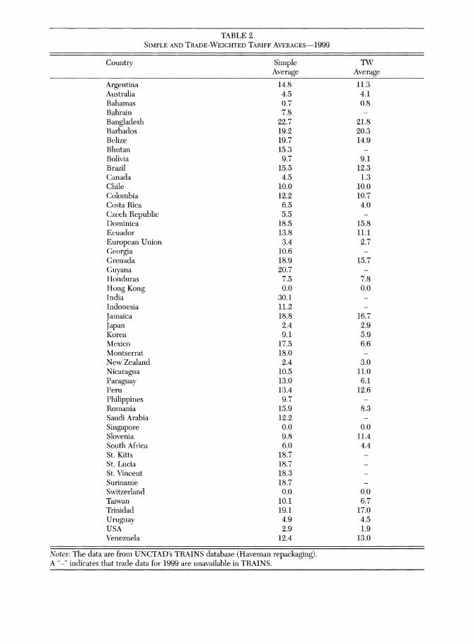
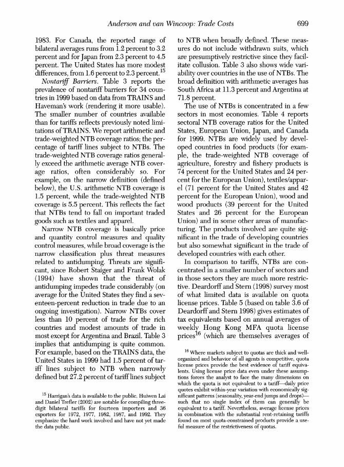


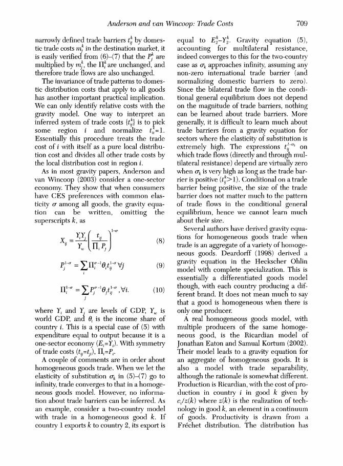

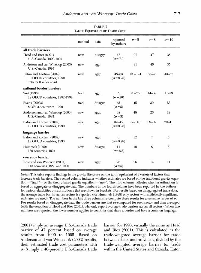


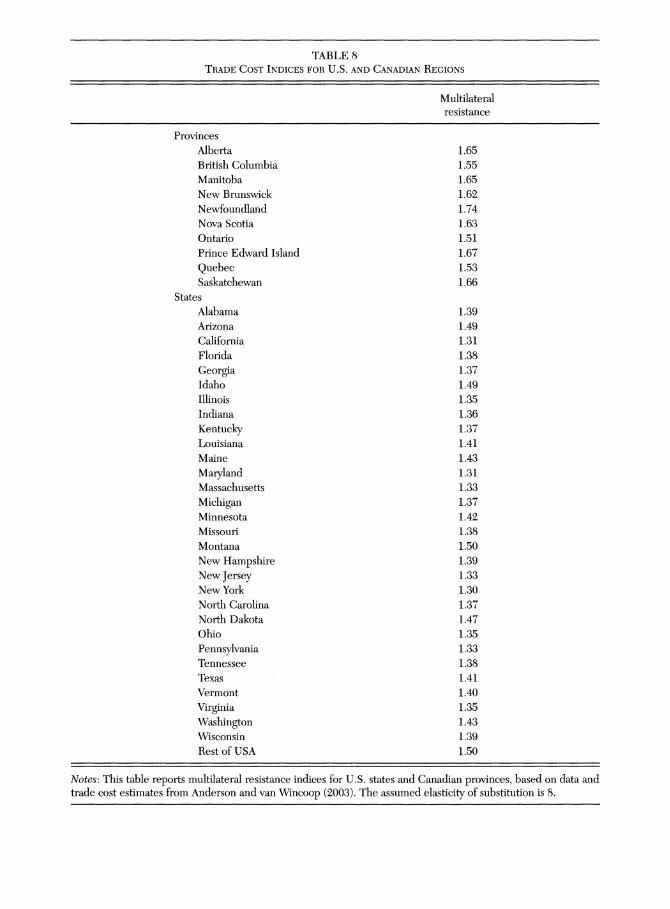


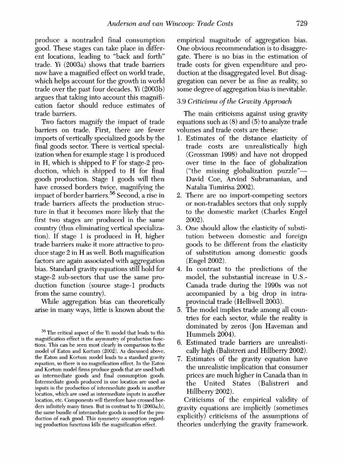


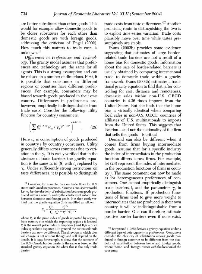

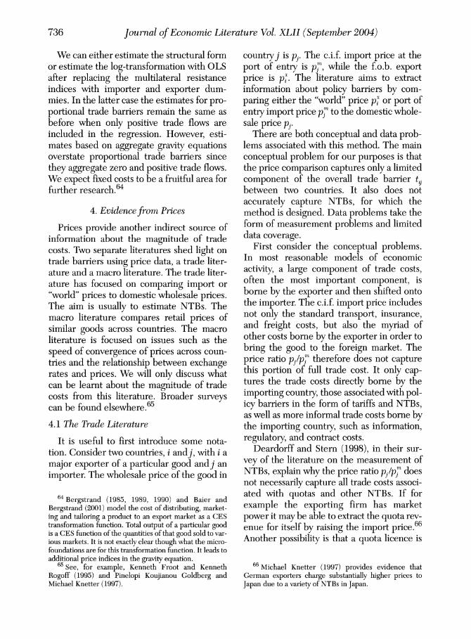
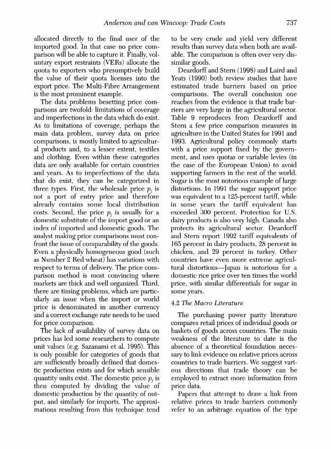
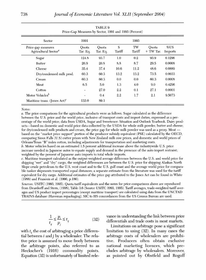


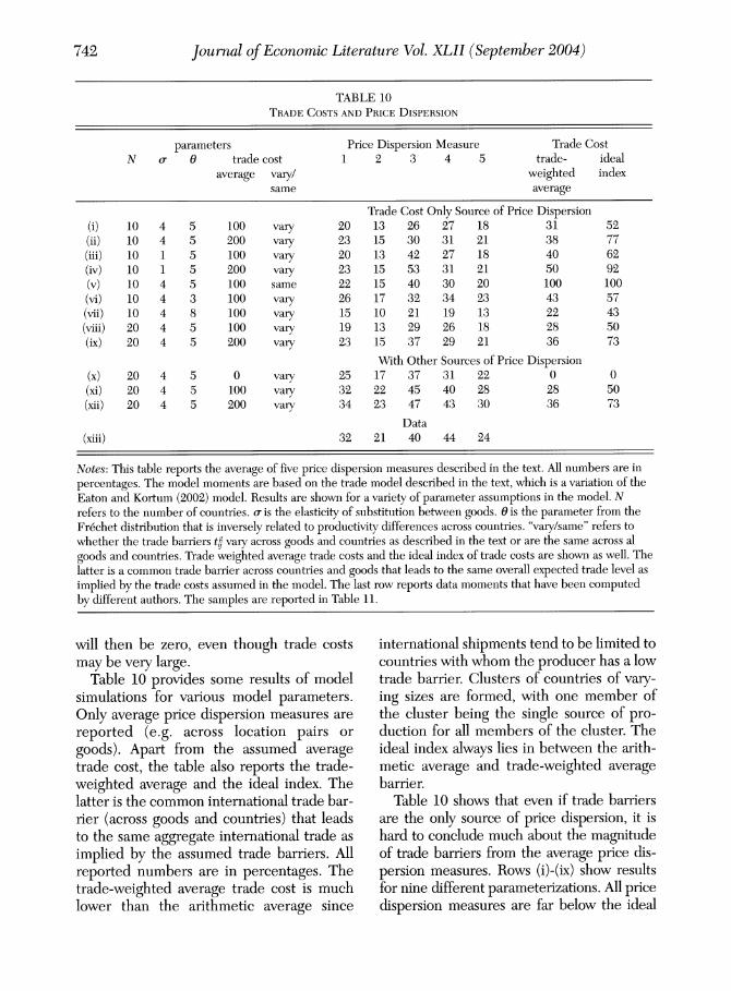
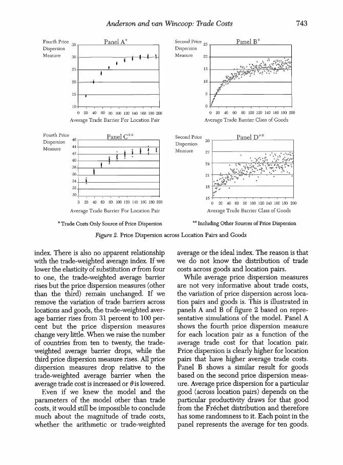
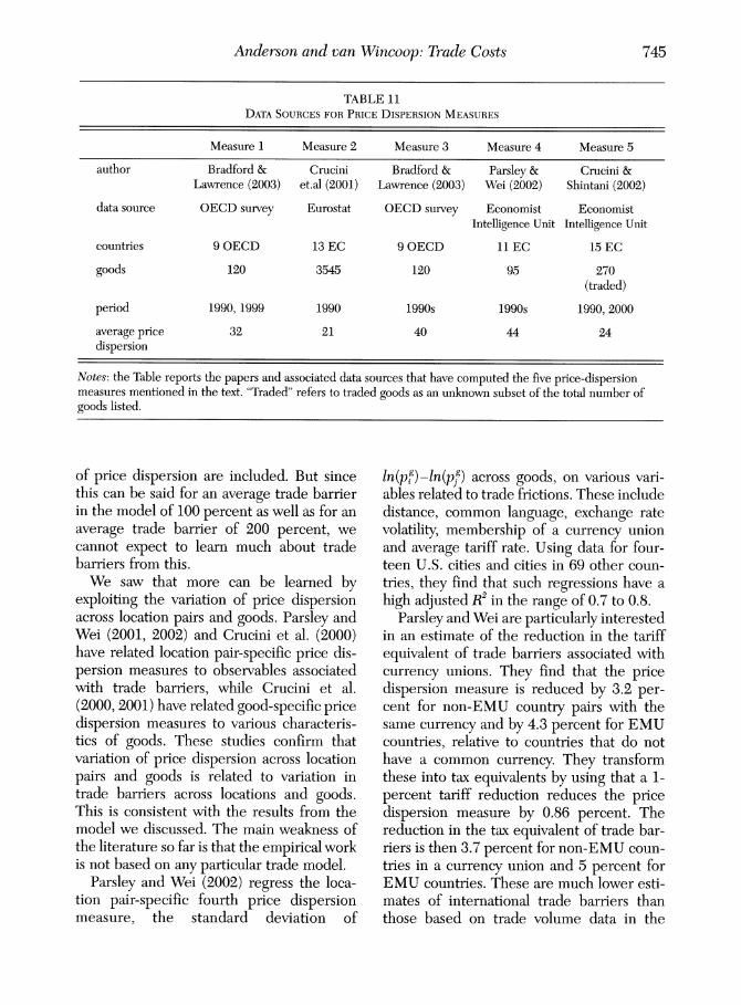


![60 Years after the Nakba: Historical Truth, Collective …...have received extensive critical reappraisal in the works of Benedict Anderson [Anderson 1991: 6, 11–2], Eric Hobsbawn](https://img.pdfslide.net/doc/110x75/5e79d74cc3e74b7c3b5034fc/60-years-after-the-nakba-historical-truth-collective-have-received-extensive.jpg)