EUROPEAN COMMISSION

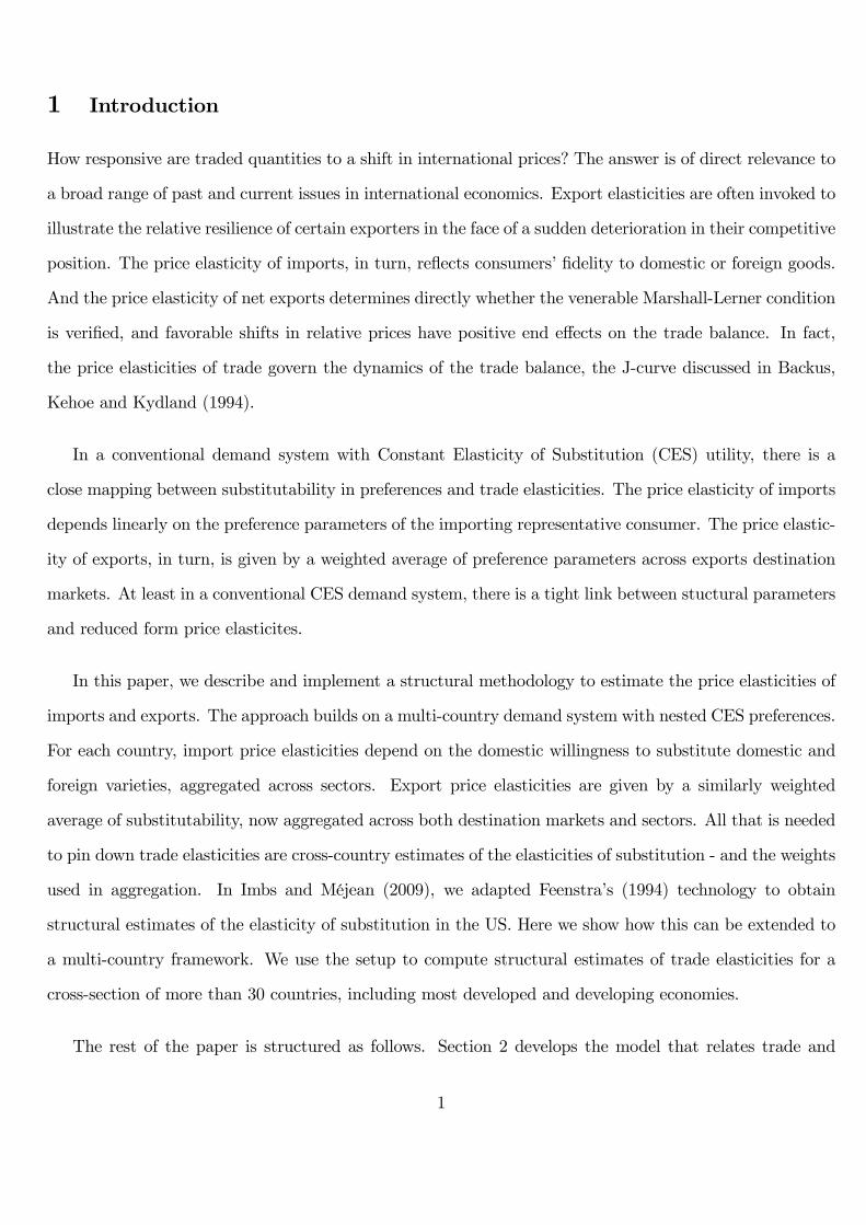
Trade ElasticitiesA Final Report for the European Commission

Jean Imbs and Isabelle Méjean

Economic Papers 432| December 2010

EUROPEAN ECONOMY

Economic Papers are written by the Staff of the Directorate-General for Economic and Financial Affairs, or by experts working in association with them. The Papers are intended to increase awareness of the technical work being done by staff and to seek comments and suggestions for further analysis. The views expressed are the author’s alone and do not necessarily correspond to those of the European Commission. Comments and enquiries should be addressed to: European Commission Directorate-General for Economic and Financial Affairs Publications B-1049 Brussels Belgium E-mail: Ecfin-Info@ec.europa.eu This paper exists in English only and can be downloaded from the website ec.europa.eu/economy_finance/publications A great deal of additional information is available on the Internet. It can be accessed through the Europa server (ec.europa.eu) KC-AI-10-432-EN-N ISSN 1725-3187 ISBN 978-92-79-14918-4 doi 10.2765/46193 © European Union, 2010 Reproduction is authorised provided the source is acknowledged.

Trade Elasticities

A Final Report for the European Commission�

Jean Imbsy Isabelle Méjeanz

July 2010

Abstract

In a demand system with conventional CES preferences, the price elasticitites of aggregate trade �ows

are weighted averages of sector-speci�c elasticities of substitution. We describe a methodology that can

be used to estimate country-speci�c values for the price elasticities of aggregate imports and exports.

We �rst use disaggregated trade data to compute structural estimates of international substitutability

for a large cross section of countries. We aggregate up the estimates using model-implied, country-

speci�c weights. We obtain structural estimates of the price elasticities of aggregate exports and

imports for more than 30 countries, including most developed and developing economies.

JEL Classi�cation Numbers: F32, F02, F15, F41

Keywords: Price Elasticity of Exports, Price Elasticity of Imports.

�Special thanks are due to Soledad Zignano for many insightful discussions and assistance with the estimations.yParis School of Economics, HEC Lausanne, Swiss Finance Institute and CEPR. Corresponding author: HEC Lausanne,

Extranef 228, Lausanne Switzerland 1015. +41 21 692 3484, jimbs@unil.ch, www.hec.unil.ch/jimbszInternational Monetary Fund, Ecole Polytechnique and CEPR, imejean@imf.org, http://www.isabellemejean.com

1 Introduction

How responsive are traded quantities to a shift in international prices? The answer is of direct relevance to

a broad range of past and current issues in international economics. Export elasticities are often invoked to

illustrate the relative resilience of certain exporters in the face of a sudden deterioration in their competitive

position. The price elasticity of imports, in turn, re�ects consumers��delity to domestic or foreign goods.

And the price elasticity of net exports determines directly whether the venerable Marshall-Lerner condition

is veri�ed, and favorable shifts in relative prices have positive end e¤ects on the trade balance. In fact,

the price elasticities of trade govern the dynamics of the trade balance, the J-curve discussed in Backus,

Kehoe and Kydland (1994).

In a conventional demand system with Constant Elasticity of Substitution (CES) utility, there is a

close mapping between substitutability in preferences and trade elasticities. The price elasticity of imports

depends linearly on the preference parameters of the importing representative consumer. The price elastic-

ity of exports, in turn, is given by a weighted average of preference parameters across exports destination

markets. At least in a conventional CES demand system, there is a tight link between stuctural parameters

and reduced form price elasticites.

In this paper, we describe and implement a structural methodology to estimate the price elasticities of

imports and exports. The approach builds on a multi-country demand system with nested CES preferences.

For each country, import price elasticities depend on the domestic willingness to substitute domestic and

foreign varieties, aggregated across sectors. Export price elasticities are given by a similarly weighted

average of substitutability, now aggregated across both destination markets and sectors. All that is needed

to pin down trade elasticities are cross-country estimates of the elasticities of substitution - and the weights

used in aggregation. In Imbs and Méjean (2009), we adapted Feenstra�s (1994) technology to obtain

structural estimates of the elasticity of substitution in the US. Here we show how this can be extended to

a multi-country framework. We use the setup to compute structural estimates of trade elasticities for a

cross-section of more than 30 countries, including most developed and developing economies.

The rest of the paper is structured as follows. Section 2 develops the model that relates trade and

1

substitution elasticities. Section 3 discusses our structural estimation of substitution elasticities across

countries, along with the data we use. Our results are presented in Section 4, and Section 5 concludes.

2 Theory

We build on a Constant Elasticity of Substitution (CES) demand system, with two layers of aggregation.

Aggregate consumption is a CES aggregate of sectors indexed by k = 1; :::; K. Each sector, in turn, is a

CES index of varieties j 2 Ikj that can be produced either at home or abroad. Consumption in country j

is given by

Cj =

24Xk2Kj

(�kjCkj) j�1 j

35 j

j�1

where �kj denotes an exogenous preference parameter and j the elasticity of substitution between sectors

in country j. Consumption in each sector is derived from a range of varieties of good k, that may be

imported or not, as in

Ckj =

24Xi2Ikj

��kij Ckij

��kj�1�kj

35�kj

�kj�1

Here i 2 Ikj indexes varieties of good k, produced in country i and consumed by country j. We let

the elasticity of substitution �kj be heterogeneous across industries and importing countries. �kij lets

preferences vary exogenously across varieties, re�ecting for instance di¤erences in quality or a home bias

in consumption.

The representative maximizing agent chooses consumption keeping in mind that all varieties incur a

transport cost � kij. In the trade literature, the transport cost is usually assumed to be zero for domestically

produced goods, i.e. � kjj = 1. Utility maximization implies that demand for variety i in each sector k is

given by

Ckij = ��kj�1kij

�PkijPkj

�1��kj 1

Pkij� j�1kj

�PkjPj

�1� jPjCj (1)

2

with

Pkij = � kijPfobkij

Pkj =

24Xi2Ikj

�Pkij�kij

�1��kj35 11��kj

Pj =

24Xk2Kj

�Pkj�kj

�1� j35 11� j

where P fobkij is the Free On Board (FOB) price of variety i. Without loss of generality, we assume FOB

prices are expressed in the importer�s currency.

We now ask our model how aggregate quantities respond to changes in aggregate international rela-

tive prices. Our aim here is to replicate the assumptions that underly conventional estimations of trade

elasticities. In macroeconomics, the conventional estimated regressions write

lnMjt = �Mj ln

PMjtPjt

!+ Yjt

lnXjt = �Xj ln

PXjtP �t

!+ Zjt

whereMjt and Xjt measure aggregate imports and exports by country j,PMjtPjtis the price of imports relative

to domestic prices in country j,PXjtP �t

is the price of exports relative to prices in the destination country,

denoted with a �, and Yjt and Zjt are country-speci�c controls. �Mj (�Xj ) measures the response of imports

(exports) to a shock in the price of imports (exports), relative to the price of the competing goods. Both

are expected to be negative.

In what follows we use these de�nitions of trade elasticities and compute the response of trade to a

shock a¤ecting all relative prices in country j, across all sectors k. Let �Mkj (�Xkj) denote the response of

country j�s sectoral imports (exports) to the shock, while �Mj (�Xj ) is the aggregate response of imports

3

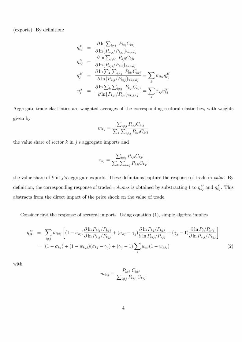
(exports). By de�nition:

�Mkj =@ ln

Pi6=j PkijCkij

@ lnfPkij=Pkjjg8k;i6=j

�Xkj =@ ln

Pi6=j PkjiCkji

@ lnfPkji=Pkiig8k;i6=j

�Mj =@ ln

Pk

Pi6=j PkijCkij

@ lnfPkij=Pkjjg8k;i6=j=Xk

mkj�Mkj

�Xj =@ ln

Pk

Pi6=j PkjiCkji

@ lnfPkji=Pkiig8k;i6=j=Xk

xkj�Xkj

Aggregate trade elasticities are weighted averages of the corresponding sectoral elasticities, with weights

given by

mkj =

Pi6=j PkijCkijP

k

Pi6=j PkijCkij

the value share of sector k in j�s aggregate imports and

xkj =

Pi6=j PkjiCkjiP

k

Pi6=j PkjiCkji

the value share of k in j�s aggregate exports. These de�nitions capture the response of trade in value. By

de�nition, the corresponding response of traded volumes is obtained by substracting 1 to �Mkj and �Xkj. This

abstracts from the direct impact of the price shock on the value of trade.

Consider �rst the response of sectoral imports. Using equation (1), simple algebra implies

�Mjk =Xi6=j

mkij

�(1� �kj)

@ lnPkij=Pkjj@ lnPkij=Pkjj

+ (�kj � j)@ lnPkj=Pkjj@ lnPkij=Pkjj

+ ( j � 1)@ lnPj=Pkjj@ lnPkij=Pkjj

�= (1� �kj) + (1� wkjj)(�kj � j) + ( j � 1)

Xk

wkj(1� wkjj) (2)

with

mkij �Pkij CkijPi6=j Pkij Ckij

4

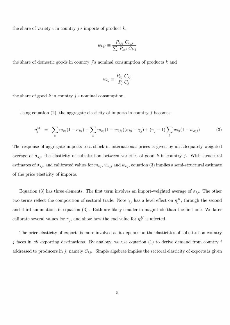
the share of variety i in country j�s imports of product k,

wkjj �Pkjj CkjjPi Pkij Ckij

the share of domestic goods in country j�s nominal consumption of products k and

wkj �Pkj CkjPj Cj

the share of good k in country j�s nominal consumption.

Using equation (2), the aggregate elasticity of imports in country j becomes:

�Mj =Xk

mkj(1� �kj) +Xk

mkj(1� wkjj)(�kj � j) + ( j � 1)Xk

wkj(1� wkjj) (3)

The response of aggregate imports to a shock in international prices is given by an adequately weighted

average of �kj, the elasticity of substitution between varieties of good k in country j. With structural

estimates of �kj, and calibrated values formkj, wkjj and wkj, equation (3) implies a semi-structural estimate

of the price elasticity of imports.

Equation (3) has three elements. The �rst term involves an import-weighted average of �kj. The other

two terms re�ect the composition of sectoral trade. Note j has a level e¤ect on �Mj , through the second

and third summations in equation (3) . Both are likely smaller in magnitude than the �rst one. We later

calibrate several values for j, and show how the end value for �Mj is a¤ected.

The price elasticity of exports is more involved as it depends on the elasticities of substitution country

j faces in all exporting destinations. By analogy, we use equation (1) to derive demand from country i

addressed to producers in j, namely Ckji. Simple algebrae implies the sectoral elasticity of exports is given

5

by

�Xjk =Xi6=j

xkji

�(1� �ki)

@ lnPkji=Pkii@ lnPkji=Pkii

+ (�ki � i)@ lnPki=Pkii@ lnPkji=Pkii

+ ( i � 1)@ lnPi=Pkii@ lnPkji=Pkii

�

=Xi6=j

xkji

"(1� �ki) + (�ki � i)wkji + ( i � 1)

Xk

wkiwkji

#(4)

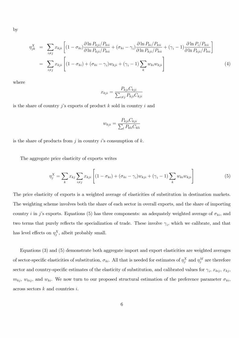
where

xkji =PkjiCkjiPi6=j PkjiCkji

is the share of country j�s exports of product k sold in country i and

wkji =PkjiCkjiPl PkliCkli

is the share of products from j in country i�s consumption of k.

The aggregate price elasticity of exports writes

�Xj =Xk

xkjXi6=j

xkji

"(1� �ki) + (�ki � i)wkji + ( i � 1)

Xk

wkiwkji

#(5)

The price elasticity of exports is a weighted average of elasticities of substitution in destination markets.

The weighting scheme involves both the share of each sector in overall exports, and the share of importing

country i in j�s exports. Equations (5) has three components: an adequately weighted average of �ki, and

two terms that purely re�ects the specialization of trade. These involve i, which we calibrate, and that

has level e¤ects on �Xj , albeit probably small.

Equations (3) and (5) demonstrate both aggregate import and export elasticities are weighted averages

of sector-speci�c elasticities of substitution, �ki. All that is needed for estimates of �Xj and �Mj are therefore

sector and country-speci�c estimates of the elasticity of substitution, and calibrated values for i, xkij, xkj,

mkj, wkij, and wki. We now turn to our proposed structural estimation of the preference parameter �ki,

across sectors k and countries i.

6

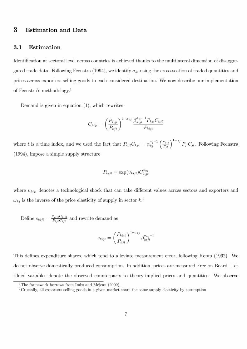
3 Estimation and Data

3.1 Estimation

Identi�cation at sectoral level across countries is achieved thanks to the multilateral dimension of disaggre-

gated trade data. Following Feenstra (1994), we identify �ki using the cross-section of traded quantities and

prices across exporters selling goods to each considered destination. We now describe our implementation

of Feenstra�s methodology.1

Demand is given in equation (1), which rewrites

Ckijt =

�PkijtPkjt

�1��kj ��kj�1kijt PkjtCkjt

Pkijt

where t is a time index, and we used the fact that PkjtCkjt = � j�1kj

�PkjtPjt

�1� jPjtCjt. Following Feenstra

(1994), impose a simple supply structure

Pkijt = exp(�kijt)C!kjkijt

where �kijt denotes a technological shock that can take di¤erent values across sectors and exporters and

!kj is the inverse of the price elasticity of supply in sector k.2

De�ne skijt =PkijtCkijtPkjtCkjt

and rewrite demand as

skijt =

�PkijtPkjt

�1��kj��kj�1kijt

This de�nes expenditure shares, which tend to alleviate measurement error, following Kemp (1962). We

do not observe domestically produced consumption. In addition, prices are measured Free on Board. Let

tilded variables denote the observed counterparts to theory-implied prices and quantities. We observe

1The framework borrows from Imbs and Méjean (2009).2Crucially, all exporters selling goods in a given market share the same supply elasticity by assumption.

7

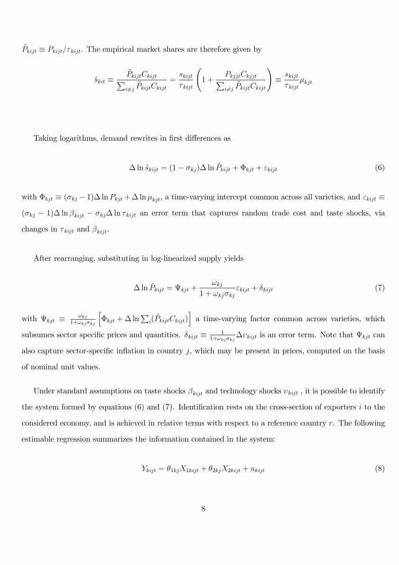
~Pkijt � Pkijt=� kijt. The empirical market shares are therefore given by

~skit �~PkijtCkijtPi6=j

~PkijtCkijt=skijt� kijt

1 +

PkjjtCkjjtPi6=j

~PkijtCkijt

!� skijt� kijt

�kjt

Taking logarithms, demand rewrites in �rst di¤erences as

� ln ~skijt = (1� �kj)� ln ~Pkijt + �kjt + "kijt (6)

with �kjt � (�kj � 1)� lnPkjt+� ln�kjt, a time-varying intercept common across all varieties, and "kijt �

(�kj � 1)� ln �kijt � �kj� ln � kijt an error term that captures random trade cost and taste shocks, via

changes in � kijt and �kijt.

After rearranging, substituting in log-linearized supply yields

� ln ~Pkijt = kjt +!kj

1 + !kj�kj"kijt + �kijt (7)

with kjt � !kj1+!kj�kj

h�kjt +� ln

Pi(~PkijtCkijt)

ia time-varying factor common across varieties, which

subsumes sector speci�c prices and quantities. �kijt � 11+!kj�kj

��kijt is an error term. Note that kjt can

also capture sector-speci�c in�ation in country j, which may be present in prices, computed on the basis

of nominal unit values.

Under standard assumptions on taste shocks �kijt and technology shocks �kijt , it is possible to identify

the system formed by equations (6) and (7). Identi�cation rests on the cross-section of exporters i to the

considered economy, and is achieved in relative terms with respect to a reference country r. The following

estimable regression summarizes the information contained in the system:

Ykijt = �1kjX1kijt + �2kjX2kijt + ukijt (8)

8

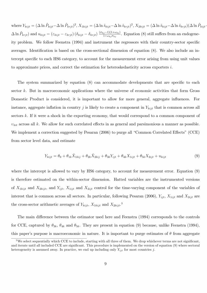
where Ykijt = (� ln ~Pkijt�� ln ~Pkrjt)2,X1kijt = (� ln ~skijt�� ln ~skrjt)2,X2kijt = (� ln ~skijt�� ln ~skrjt)(� ln ~Pkijt�

� ln ~Pkrjt) and ukijt = ("kijt � "krjt) (�kijt � �krjt) (�kj�1)(1+!kj)1+!kj�kj. Equation (8) still su¤ers from an endogene-

ity problem. We follow Feenstra (1994) and instrument the regressors with their country-sector speci�c

averages. Identi�cation is based on the cross-sectional dimension of equation (8). We also include an in-

tercept speci�c to each HS6 category, to account for the measurement error arising from using unit values

to approximate prices, and correct the estimation for heteroskedasticity across exporters i.

The system summarized by equation (8) can accommodate developments that are speci�c to each

sector k. But in macroeconomic applications where the universe of economic activities that form Gross

Domestic Product is considered, it is important to allow for more general, aggregate in�uences. For

instance, aggregate in�ation in country j is likely to create a component in Ykijt that is common across all

sectors k. If it were a shock in the exporting economy, that would correspond to a common component of

�kit across all k. We allow for such correlated e¤ects in as general and parsimonious a manner as possible.

We implement a correction suggested by Pesaran (2006) to purge all �Common Correlated E¤ects�(CCE)

from sector level data, and estimate

Ykijt = �0 + �1kX̂1kij + �2kX̂2kij + �3kYijt + �4kX1ijt + �5kX2ijt + ukijt (9)

where the intercept is allowed to vary by HS6 category, to account for measurement error. Equation (9)

is therefore estimated on the within-sector dimension. Hatted variables are the instrumented versions

of X1kijt and X2kijt, and Yijt, X1ijt and X2ijt control for the time-varying component of the variables of

interest that is common across all sectors. In particular, following Pesaran (2006), Yijt, X1ijt and X2ijt are

the cross-sector arithmetic averages of Ykijt, X1kijt and X2kijt.3

The main di¤erence between the estimator used here and Feenstra (1994) corresponds to the controls

for CCE, captured by �3k, �4k and �5k. They are present in equation (9) because, unlike Feenstra (1994),

this paper�s purpose is macroeconomic in nature. It is important to purge estimates of � from aggregate

3We select sequentially which CCE to include, starting with all three of them. We drop whichever terms are not signi�cant,and iterate until all included CCE are signi�cant. This procedure is implemented on the version of equation (9) where sectoralheterogeneity is assumed away. In practice, we end up including only Yijt for most countries j.

9

in�uences at the sector level, since not doing so would result in double-counting across the panel of sectors.

In practice we let the data tell us which CCE are e¤ectively signi�cant for each country j, and modify

speci�cation (9) accordingly.

Estimates of equation (8) map directly with the parameters of interest, since

�1kj =!kj

(�kj � 1)(1 + !kj); �2kj =

!kj�kj � 2!kj � 1(�kj � 1)(1 + !kj)

With consistent, country- and sector-speci�c estimates of �1kj and �2kj, it is straightforward to infer the

parameters of interest. In particular, the model implies

�̂kj = 1 +�̂2kj +�kj

2�̂1kjif �̂1kj > 0 and �̂1kj + �̂2kj < 1 (10)

�̂kj = 1 +�̂2kj ��kj

2�̂1kjif �̂1kj < 0 and �̂1kj + �̂2kj > 1

with �kj =

q�̂2

2kj + 4�̂1kj. Standard deviations are obtained using a �rst-order approximation around

these point estimates.4

With consistent estimates of �kj, we can infer values for the aggregate import and export price elasticities

using equations (3) and (5). We can feed the de�nitions of both trade elasticities with estimates of �̂kj that

vary by sector and by country. Then equations (3) and (5) can be used to decompose the international

di¤erences in �Mj and �Xj . We can also estimate a version of equation (8) where the elasticities of substitution

are constrained to sectoral homogeneity, i.e. �kj = �j. We now discuss the di¤erences that makes.

3.2 Heterogeneity Bias

Estimates of �Xj and �Mj have di¤erent interpretations depending on whether they are computed on the

basis of heterogeneous values of �̂kj, or using estimates constrained to homogeneity across sectors. In

4As is apparent, there are combinations of estimates in equation (10) that do not correspond to any theoretically consistentestimates of �̂kj . We follow Broda and Weinstein (2006) and use a search algorithm that minimizes the sum of squaredresiduals in equation (10) over the intervals of admissible values of the elasticities. The standard errors are bootstrapped inthese instances.

10

Imbs and Méjean (2009), we argue constrained estimates su¤er from a heterogeneity bias. The end value

obtained for �̂j does not necessarily re�ect a weighted average of sector-speci�c estimates that is grounded

in theory. This can be a problem for the calibration choice of a representative agent in general equilibrium.

A representative agent whose preferences are to re�ect the heterogeneity in substitution elasticities across

sectors should be endowed with an adequately weighted average of �̂kj, not with the value obtained for

�̂j. We show in Imbs and Méjean (2009) that using aggregate data in fact constrains estimates of �̂kj to

homogeneity across sectors. As a result, we argue estimates based on aggregate data should not be used

to calibrate the elasticity of substitution of a representative agent in an international context.

In this paper, our purpose is di¤erent. We are after estimates of reduced form elasticities, inferred from

the calibration of theory-implied weighting schemes, applied to structural estimates of �, the elasticity of

substitution. Since we are concerned with reduced form elasticities, the possibility of a heterogeneity bias

in constrained estimates of �̂j only matters in as much as it alters the end interpretation of �Mj and �Xj .

In particular, if it is aggregate data that the estimates of �Mj and �Xj are to replicate, then constrained

estimates of �̂j are of the essence. Identi�cation issues notwithstanding, the elasticity of imports (or

exports) to a shift in relative prices, that is estimated on aggregate data implicitly imposes that �̂kj = �̂j

for all k. The intuition is straightforward. Aggregating the data suppresses mechanically any sectoral

dimension from the estimation, which may result in di¤erent results than aggregating sectoral estimates.

If a discrepancy exists, there is a heterogeneity bias, and it is caused by the assumption that �̂kj = �̂j in

macro data. In that case, the behavior of macro data can only be mimicked by constrained estimates of

�̂j, fed into �Mj and �Xj .5

In contrast, the values of �Mj and �Xj based on heterogeneous estimates of �̂kj cannot hope to reproduce

the dynamic response of aggregate trade to price shocks. But they are informative nonetheless. Constrained

trade elasticities do not depend on the specialization of trade, simply because the weighting schemes in

equations (3) and (5) become largely innocuous if �̂kj = �̂j. Unconstrained trade elasticities, on the other

hand, will take di¤erent values depending on the specialization of production and trade across sectors. The

5To be precise, we show in Imbs and Méjean (2009) that aggregate data in fact assumes �̂kj = �̂j = j , since with macroaggregates, di¤erent sectors become impossible to di¤erentiate from each other. There is however nothing we can say aboutthe empirical value of j , which we calibrate throughout the paper.

11

unconstrained estimate of �Xj will take larger values in countries specialized in substitutable exports, but

not necessarily its constrained counterpart. Since the two alternatives are conceptually di¤erent, we report

both variants in this report.

The sectoral dimension plays another important role. Disaggregated data lend power to our estimation,

so that we are able to identify with precision country-speci�c estimates. In contrast, the conventional

literature has often had to use cross-country data to identify one parameter, typically assumed to be the

same for all considered countries. The assumption is almost certainly not innoucous. Anecdotal evidence

is plentiful that the elasticity is actually heterogeneous across countries. There are observable di¤erences

in the trade performance of Euro-zone countries in response to a given Euro appreciation. Journalistic

discussions are frequent, for instance of the di¤erences between resilient German and French exports. And

in general, global shocks to international relative prices do not appear to have identical consequences

across countries. The entry of China in world markets, and the accompanying fall in the relative price of

Chinese goods, has not a¤ected trade balances identically everywhere. Yet, these international di¤erences

are absent from most modelling choices in academia or policy circles. We conjecture such is the case for

lack of reliable estimates across countries.

3.3 Data

A structural estimate of �̂j requires that we observe the cross-section of imported quantities and unit values

at the sector level, and for all countries j. We choose to use the multilateral trade database ComTrade,

released by the United Nations. The data traces multilateral trade at the 6-digit level of the harmonized

system (HS6), and cover around 5,000 products for a large cross-section of countries. We focus on the

recent period, and use yearly data between 1995 and 2004. We start in 1995, as before then the number of

reporting countries displayed substantial variation. In addition, the unit values reported in ComTrade after

2004 display large time variations that seem to correspond to a structural break. The database is freely

available online, to facilitate replication of our results. We focus on the data based on export declarations,

to maximize country coverage.

12

Thanks to the multilateral dimension of our data, we are able to estimate �̂j for a wide range of countries

j. Identi�cation requires the cross-section of countries exporting to j be wide enough, for all sectors. And

since the precision of our estimates depends on the time-average of these trade data, we also need the cross-

section of exporting countries (and goods) to be as stable over time as possible. We therefore only retain

goods for which a minimum of 20 exporting countries are available throughout the period we consider. In

addition, both unit values and market shares are notoriously plagued by measurement error. We limit the

in�uence of outliers, and compute the median growth rate at the sector level for each variable, across all

countries and years. We exclude the bilateral trade �ows for all sectors whose growth rates exceed �ve time

that median value in either unit values or in market share. On average, the resulting truncated sample

covers about 85 percent of world trade. Table 1 presents some summary statistics for the 33 countries we

have data for. The number of sectors ranges from 10 to 26. We also report the total number of exporters

into each country j, equal to the product of the number of sectors in country j, times the number of

exporters for each sectors. This suggests the average number of exporters ranges from 35 in Sri Lanka

to more than 90 in the United States. For each sector, our data implies an average number of exporting

countries of 53.

The main constraint on the range of countries for which we can obtain end estimates of �Xj and �Mj is

not imposed by the availability of trade data. It is the calibration of sectoral shares that is limited by the

availability of adequate data. Computing aggregate trade elasticities requires the calibration of six weights.

We need values for mkj and xkj, which denote the value share of sector k in the aggregate imports and

exports of country j, respectively. We need a value for xkji, which is the share of country j�s exports of

product k sold in country i. There are also three consumption shares: wkj, which denotes the share of

sector k in country j�s nominal consumption, wkjj, the share of domestically produced goods in sector k

consumption, and wkji, the share of sector k consumption in country i that is imported from country j.

Consumption data require information on domestic production at sectoral level, across as large a cross-

section of countries as possible. This is absent from conventional international trade databases. We resort

instead to UNIDO data, which report nominal sectoral output at the 3-digit ISIC (revision 2) level. UNIDO

data are incomplete for some countries. Since aggregation can become misleading for countries where too

13

few sectors are reported, we impose a minimum of 10 sectors for all countries j. This tends to exclude

small or developing economies, such as Hong Kong, Panama, Slovakia or Poland. The data are expressed in

USD, and available at a yearly frequency. To limit the consequences of measurement error, we use �ve-year

averages of the relevant UNIDO data. We experiment with weights computed between 1991 and 1995, or

between 1996 and 2000. We merge multilateral trade data into the ISIC classi�cation.

The UNIDO dataset is focused on manufacturing goods only, which truncates somewhat the original

coverage in trade data. But the vast majority of traded goods are manufactures, so that the sampling

remains minimal. We have experimented with weights implied by the OECD Structural Analysis database

(STAN): for countries covered by both datasets, the end elasticities were in fact virtually identical - even

though STAN provides information on all sectors of the economy. UNIDO has sectoral information on

many more countries, not least non-OECD members like China. Such coverage is important in its own

right, but it is also of the essence when it comes to computing export elasticities. The price elasticity of

exports involves an average across destination markets for all countries considered. Focusing on just OECD

economies would complicate the interpretation of our end estimates, as they would ignore non-OECD trade

�ows, which have increased in magnitude of late. The last column in Table 1 reports the percentage of

total trade as implied by ComTrade, that we continue to cover once we restrict the sample to sectors for

which we have UNIDO data. The coverage is below 20 percent for small open economies such as Hong

Kong, Singapore, or the Philippines, and around three-quarters for large developed economies such as the

US, France or Spain.

The values for mkj and xkj are calculated as the ratios of sectoral imports and exports, relative to their

respective aggregate at the country level. The value for xkji is computed as the ratio of good k�s exports

from country j that are sold in i. A choice must be made when it comes to the sectors used in computing

xkj. A �rst option is to consider the coverage in ComTrade data for both mkj and xkj , but without any

guarantee they are the same. Such choice implies that we allow for the sectoral patterns of exports from

country j to di¤er from what it imports. The assumption seems realistic and plausible, but it takes missing

data from ComTrade at face value - even though data collection issues or measurement error may in reality

be the reason why a sector is missing from ComTrade. In addition, the choice also implies that the trade

14

weights xkj are computed on a di¤erent sample than the consumption weights. This may create issues of

comparability, as the consumption weights are constructed on the basis of a sectoral coverage put together

by Di Giovanni and Levchenko (2009), with a view to accounting for outliers.

An alternative is to use the trade data compiled by Di Giovanni and Levchenko (2009), and e¤ectively

imposing no specialization, as countries import and export the same sectors. The assumption is clearly at

odds with the evidence, but it is prudent. There are many sectors with zero entries in disaggregated trade

data, and the distinction between e¤ectively non traded goods, measurement error, or improvement in data

collection over time is often di¢ cult. With a no-specialization assumption, we maximize the comparability

of our estimates of trade elasticities on the import and the export sides. This is done at the potential cost

of realism.

For the three other weights, we require information on both production and trade at the sectoral level.

In order to maximize concordance and comparability, we use a dataset built by Di Giovanni and Levchenko

(2009) who merge information on production from UNIDO and on bilateral trade �ows from the World

Trade Database compiled by Feenstra et al (2005). Domestic consumption at the sectoral level is computed

as production net of exports, and overall consumption is production net of exports but inclusive of imports.

We have

wkjj �Ykj �Xkj

Ykj �Xkj +Mkj

where Xkj (Mkj) denotes country j�s exports (imports) of good k.

wkji =Xkji

Yki �Xki +Mki

=xkjiPj xkji

(1� wkii)

where Xkji are country j�s exports of good k sold in country i. And

wkj �Ykj �Xkj +MkjPk (Ykj �Xkj +Mkj)

We experimented with alternative combinations of data sources. Rather than using the dataset merged

by Di Giovanni and Levchenko (2009), we combined data from ComTrade for sectoral imports or exports,

15

and from UNIDO for output. In all instances, however, we made use of output data corresponding to

the UNIDO data treated for outliers by Di Giovanni and Levchenko (2009). This is important, for it

ensures the compatibility of production and trade data, and the meaningfulness of the measures w of local

consumption. We did however use production data from the OECD STAN as well, with substantially

smaller country coverage. For those countries where data are available across all three alternatives, our

end results are virtually unchanged.

4 Results

We present �rst cross-country estimates of import elasticities. We then turn to exports. In both instances,

we report elasticity estimates obtained from both constrained and unconstrained estimates of the preference

parameter �kj. We also present extensive robustness analysis. We consider di¤erent calibrated values for

the cross-sector elasticity of substitution , and use di¤erent sub-periods to compute the weights w, m and

x.

4.1 Import Price Elasticities

Table 2 reports the constrained estimates of �Mj for 33 countries at various levels of development. The

elasticities are computed imposing = 1. The left panel of the table uses weights computed on the basis

of a 5-year average between 1991 and 1995. There is a lot of heterogeneity across countries, with values

ranging from 0:5 in Hong Kong to 2:7 in Italy or Finland. Small, open countries tend to display low

elasticities, with Hong Kong, Singapore or Austria all taking values around 1. Large, rich economies tend

to have high elasticities, with France, the US, Spain, Japan, Australia or Italy all around 2.

Commodity exporters tend to have large elasticities, with elasticitites above 1:5 for Venezuela, Australia,

or Indonesia. The exception is Kuwait, which takes one of the lowest values in our sample, at 0:6. Kuwait

is extremely specialized in oil products, and is probably an outlier in that sense. There is no apparent

mapping between income per capita and import elasticities, as there are developed countries at both ends

of the distribution. The import elasticity in China is estimated at 1:57, with a tight standard error of 0:2.

16

In the US and Japan, the import elasticity is closer to 2, with standard errors below 0:2. The big European

economies have estimates in the same region - with French, Spanish and German elasticities at or around 2.

The value for Italy is higher, at 2:7, although the estimate is less precise with standard errors equal to 0:4.

Small European economies tend to have low elasticities: Greece and Austria are below 1, Hungary, Norway,

the UK and Portugal are close to 1:5. The main lesson from Table 2 is a large cross-country heterogeneity.

The estimated elasticities change little when weights used in aggregation are measured over the end of

the 1990�s, between 1996 and 2000. For the countries with observations in both sub-periods, the discrepancy

between the values on the left and right panels of Table 1 is virtually never signi�cant, compared to the

standard deviations reported in the table. Exceptions are Canada, whose elasticity falls from 1:79 to 1:36,

Australia, which goes from 2:04 to 1:54, and perhaps Israel and Germany, which go from 2:19 to 1:54 and

1:72 to 1:34, respectively. In general, the magnitude and ranking of import elasticities are largely robust

to aggregation weights that are computed over di¤erent time periods. Of course, this can re�ect the well

known persistence in international trade patterns - even though the 1990�s saw the rapid emergence of

China in world trade.

Table 3 presents the unconstrained estimates of �Mj for the same parametrization. Estimates are now

substantially more heterogeneous, ranging from 0:7 to 7:14. Interestingly, the ranking of countries is altered

somewhat. There is now a clear tendency for large, emerging markets to have high elasticity values. China

is the most striking, that now tops the ranking of 33 countries with an elasticity estimate of 7:14. The

same can be said of India, Korea, or Turkey. Rich developed countries now tend to be at the bottom of

the distribution, with elasticity estimates below 3. This di¤erence in ranking re�ects the importance of

specialization in driving the (unconstrained) elasticity of imports. Rich countries tend to import goods that

are not substitutable, whereas the opposite can be said of large developing economies. Such importance of

specialization was not apparent from Table 2. These relative rankings remain virtually unchanged when

the weighting scheme is chosen using data from the second half of the 1990�s.

Tables 4 and 5 present the constrained and unconstrained estimates of �Mj for = 2. Goods across

sectors are now assumed to be substitutes. From equation (3), we expect alternative values of to have a

minimal impact on the level of aggregate trade elasticities. The two Tables con�rm this to be the case. The

17

magnitudes and distribution of elasticities in Table 4 resembles Table 2, and unconstrained estimates in

Table 5 are virtually identical to Table 3. In particular, the same two results obtain. Constrained estimates

are relatively less heterogeneous. And unconstrained estimates re�ect di¤erences in income per capita, and

presumably of the specialization of production and trade. The same can be said for estimates implied by

a calibration of = 0:5, which are reported in Tables 6 and 7.

4.2 Export Price Elasticities

Computing the price elasticities of exports entails averaging across two dimensions: across sectors, and

across destination markets. The latter is performed with the weights xkji, which capture the international

allocation of exports from country j. We only estimate substitution elasticities for the destination countries

in our sample, so thatP

i6=j xkji is in fact not unity in our data. In what follows, we experiment both with

and without normalization , i.e. report estimates of �Xj arising from the actual weights xkji that we observe,

and also from weights that are normalized so thatP

i6=j xkji = 1. The normalization amounts to assuming

the export markets we do not observe are in fact negligible in country j�s trade.

Table 8 reports constrained estimates of the export elasticity for 33 countries, where we do not nor-

malizeP

i6=j xkji to unity, and use the UNIDO coverage to compute the export weights xkj, i.e. we assume

specialization away. Estimates correspond to = 1. Table 9 reports the corresponding unconstrained elas-

ticities. Constrained estimates display some heterogeneity, with values ranging from 0:9 to 2:25. Developed

countries tend to take relatively low values, with Singapore, the US, Germany, the UK, Japan, France or

Austria all around 1:5. Small open economies, such as Canada, Portugal, Hong Kong or Israel take larger

values, around 2. Using weights from the late 90�s does not alter these magnitudes, nor indeed the ranking.

As with import elasticities, heterogeneity is magni�ed for unconstrained elasticities. Estimates in Table

9 now range from 1:43 to 5:21. The ranking of countries remains however largely unchanged, with developed

countries taking relatively low values. Interestingly, both India and China have export elasticities that are

similar in magnitude with the US, France, the UK, or more generally rich OECD economies. This result

18

does not depend on whether estimates are constrained or unconstrained. Unconstrained export elasticities

are highest once again for small open economies, with Australia, Canada and Hong Kong taking the highest

three values. Using weights from the late 1990�s barely alters these results, with the possible exception of

the German elasticity that increases signi�cantly, whereas Korea�s and Israel�s fall in absolute value.

Tables 10 and 11 impose the normalization thatP

i6=j xkji = 1, but continue to use the same sectoral

coverage for xkj as is done for import elasticities. As expected, the normalization has level e¤ects on all

estimates, since xkji now take higher values for all countries. Constrained estimates now range from 1:9 to

3:0, whereas unconstrained estimates range from 3:5 to 6:0. Unconstrained estimates continue to display

higher heterogeneity. In addition, the ranking of countries is altered. With the exception of China, which

takes the lowest value in both Tables, the rank correlation between income per capita and �Xj (in absolute

value) is now �rmly negative. Rich countries take relatively low values, as one would expect from countries

that export branded, di¤erentiated goods. Poor countries, and small open economies tend to take high

values - in a way that is even more apparent for the unconstrained estimates in Table 11. The case of

China is intriguing, and its ranking changes drastically compared with Tables 8 and 9. An explanation may

lie in the fact that imposingP

i6=j xkji = 1 in fact assumes our data actually contains all export markets

of country j. The di¤erence between the estimates reported in Tables 8 and 10 will be largest, the more

imperfect our actual coverage. Estimates of �Xj for China in fact increase little between Tables 8 and 10,

which suggests our coverage of China�s trade may in fact be substantially better than what it is for other

countries, where estimates of �Xj increase more. In fact, the coverage percentages reported in Table 1 do

suggest that, amongst developing economies, Chinese data have relatively high coverage, almost equal to

50% of all available trade �ows in ComTrade. To limit the incidence of cross-country di¤erences in coverage

on our elasticity estimates, we do not imposeP

i6=j xkji = 1 in what follows.

Tables 12 and 13 report elasticity estimates imposing sectoral specialization as implied by ComTrade

data. Comparing Tables 12 and 8, it is patent that using ComTrade data has little consequence on the

magnitude and ranking of elasticity estimates. �Xj range from 0:91 to 2:25 in Table 8 (without special-

ization), and from 1:02 to 2:24 in Table 12. Di¤erences in ranking are too small to detect, and estimates

for most big economies are virtually identical. The comparison between Tables 9 and 13 implies similar

19

comments, with only one noticeable change, namely Venezuela�s elasticity doubling to 6:7 when specializa-

tion is imposed. This suggests the assumption that Venezuela imports and exports in the same sectors is

especially implausible.

Tables 14, 15, 16 and 17 report estimates for = 2, or = 0:5, while maintaining the specialization

hypothesis. The elasticity estimates are virtually unchanged, and country rankings continue to have the

properties discussed previously. Di¤erent calibrates values for seem to have little e¤ects on the end

estimates of �Xj .

5 Conclusion

We describe a CES demand system where the price elasticities of exports and imports are given by weighted

averages of the international elasticity of substitution. We adapt the econometric methodology in Feenstra

(1994) and Imbs and Méjean (2009) to estimate structurally the substitution elasticity for a broad range of

countries. We collect from a variety of sources the weights that theory implies should be used to infer both

imports and exports elasticities. We report trade elasticity estimates for more than 30 countries, including

most developed and the major developing economies. We �nd susbtantial cross-country dispersion, which

is robust to alternative measurement strategies. Our benchmark calibration imply constrained import

elasticitites ranging from 0:5 to 2:7. While constrained import elasticities display little cross-country corre-

lation with income per capita, unconstrained elasticities are clearly higher for open, developing, specialized

economies - and closer to 0 in rich countries. Export elasticities display relatively less dispersion, and range

(in absolute value) from 0:9 to 2:25. Rich open economies tend to take low absolute values, and developing

countries have relatively high estimates. Alternative calibration choices for the cross-sector elasticity

have little end consequences on trade elasticities. The same is true of the period used to calibrate the

weights used in aggregating elasticities of substitution.

20

6 References

Backus, D., P. Kehoe & F. Kydland, 1994, �Dynamics of the Trade Balance and the Terms of Trade:

The J-Curve?�American Economic Review, 84(1): 84-103.

Broda, C. & D. Weinstein, 2006, �Globalization and the Gains from Variety�, The Quarterly Journal

of Economics, 121(2): 541-585

Di Giovanni, J. & A. Levchenko, 2009, �Trade Openness and Volatility�, Review of Economics and

Statistics, 91(3): 558-85.

Feenstra, R., 1994, �New Product Varieties and the Measurement of International Prices�, American

Economic Review, 84(1): 157-177.

Imbs, J. & Mejean, I., 2009, �Elasticity Optimism�, CEPR Discussion Papers, 7177.

Kemp, M., 1962, �Error of Measurements and Bias in Estimates of Import Demand Parameters�, Eco-

nomic Record, 38: 369-372.

Pesaran, H., 2006, �Estimation and Inference in Large Heterogeneous Panels with a Multifactor Error

Structure�, Econometrica, 74(4): 967-1012.

21

Table 1: Summary Statistics

Weights 1991-1995 Weights 1996-2000# sect # sect�exp % Trade # sect # sect�exp % Trade

Australia 16 763 47.7 18 851 50.1Austria 24 1127 69.5 19 898 60.9Belgium 13 857 24.7Canada 24 1415 63.0 24 1415 63.0Sri Lanka 10 355 24.3 10 355 24.3China 18 989 49.3 17 924 35.3Finland 25 1116 61.0 22 998 59.8France 25 1950 74.0 26 2007 74.1Germany 20 1506 50.4 21 1602 65.7Greece 17 904 47.1Hong Kong 11 596 15.3Hungary 19 856 44.5 15 667 18.8Indonesia 14 575 39.5Israel 20 868 38.7 14 620 32.6Italy 25 1854 71.3 26 1918 72.6Japan 26 1470 61.4 26 1470 61.4Korea 25 1170 54.6 25 1170 54.6Kuwait 15 640 24.6 13 559 21.7Taiwan 20 972 40.3Norway 20 904 48.7 23 1029 51.4Philippines 15 589 17.1Poland 23 1113 63.6Portugal 22 1029 64.4 26 1194 70.6India 17 884 38.1 17 884 38.1Singapore 10 496 12.3Slovakia 10 369 23.4Spain 26 1725 75.1 26 1725 75.1Sweden 25 1305 72.0 21 1067 54.0Turkey 23 1182 53.1 20 1020 48.9Egypt 19 925 37.7United Kingdom 26 2015 77.4 24 1838 73.0United States 26 2347 77.1 25 2258 76.7Venezuela 20 758 37.1

22

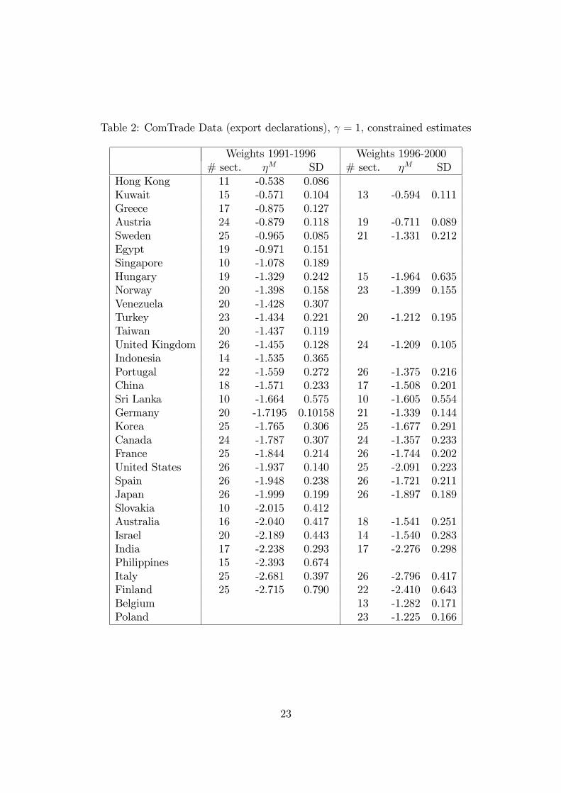
Table 2: ComTrade Data (export declarations), = 1, constrained estimates

Weights 1991-1996 Weights 1996-2000# sect. �M SD # sect. �M SD

Hong Kong 11 -0.538 0.086Kuwait 15 -0.571 0.104 13 -0.594 0.111Greece 17 -0.875 0.127Austria 24 -0.879 0.118 19 -0.711 0.089Sweden 25 -0.965 0.085 21 -1.331 0.212Egypt 19 -0.971 0.151Singapore 10 -1.078 0.189Hungary 19 -1.329 0.242 15 -1.964 0.635Norway 20 -1.398 0.158 23 -1.399 0.155Venezuela 20 -1.428 0.307Turkey 23 -1.434 0.221 20 -1.212 0.195Taiwan 20 -1.437 0.119United Kingdom 26 -1.455 0.128 24 -1.209 0.105Indonesia 14 -1.535 0.365Portugal 22 -1.559 0.272 26 -1.375 0.216China 18 -1.571 0.233 17 -1.508 0.201Sri Lanka 10 -1.664 0.575 10 -1.605 0.554Germany 20 -1.7195 0.10158 21 -1.339 0.144Korea 25 -1.765 0.306 25 -1.677 0.291Canada 24 -1.787 0.307 24 -1.357 0.233France 25 -1.844 0.214 26 -1.744 0.202United States 26 -1.937 0.140 25 -2.091 0.223Spain 26 -1.948 0.238 26 -1.721 0.211Japan 26 -1.999 0.199 26 -1.897 0.189Slovakia 10 -2.015 0.412Australia 16 -2.040 0.417 18 -1.541 0.251Israel 20 -2.189 0.443 14 -1.540 0.283India 17 -2.238 0.293 17 -2.276 0.298Philippines 15 -2.393 0.674Italy 25 -2.681 0.397 26 -2.796 0.417Finland 25 -2.715 0.790 22 -2.410 0.643Belgium 13 -1.282 0.171Poland 23 -1.225 0.166

23

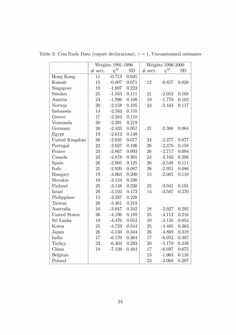
Table 3: ComTrade Data (export declarations), = 1, Unconstrained estimates

Weights 1991-1996 Weights 1996-2000# sect. �M SD # sect. �M SD

Hong Kong 11 -0.713 0.045Kuwait 15 -0.807 0.071 12 -0.857 0.020Singapore 10 -1.697 0.223Sweden 25 -1.943 0.111 21 -2.052 0.168Austria 24 -1.996 0.108 19 -1.778 0.102Norway 20 -2.158 0.105 23 -2.443 0.117Indonesia 14 -2.163 0.155Greece 17 -2.283 0.110Venezuela 20 -2.391 0.219Germany 20 -2.433 0.057 21 -2.386 0.064Egypt 19 -2.613 0.148United Kingdom 26 -2.635 0.077 24 -2.277 0.077Portugal 22 -2.637 0.196 26 -2.370 0.158France 25 -2.867 0.093 26 -2.717 0.094Canada 24 -2.878 0.301 24 -2.163 0.206Spain 26 -2.905 0.125 26 -2.548 0.111Italy 25 -2.920 0.087 26 -2.951 0.086Hungary 19 -3.063 0.200 15 -2.085 0.110Slovakia 10 -3.124 0.238Finland 25 -3.148 0.230 22 -3.041 0.191Israel 20 -3.193 0.173 14 -3.587 0.270Philippines 15 -3.337 0.228Taiwan 20 -3.461 0.219Australia 16 -3.647 0.342 18 -2.927 0.292United States 26 -4.196 0.189 25 -4.112 0.216Sri Lanka 10 -4.476 0.052 10 -4.135 0.054Korea 25 -4.723 0.344 25 -4.485 0.363Japan 26 -5.150 0.344 26 -4.869 0.319India 17 -6.170 0.384 17 -6.052 0.397Turkey 23 -6.403 0.293 20 -5.179 0.239China 18 -7.139 0.484 17 -6.697 0.675Belgium 13 -1.963 0.116Poland 23 -3.069 0.207

24

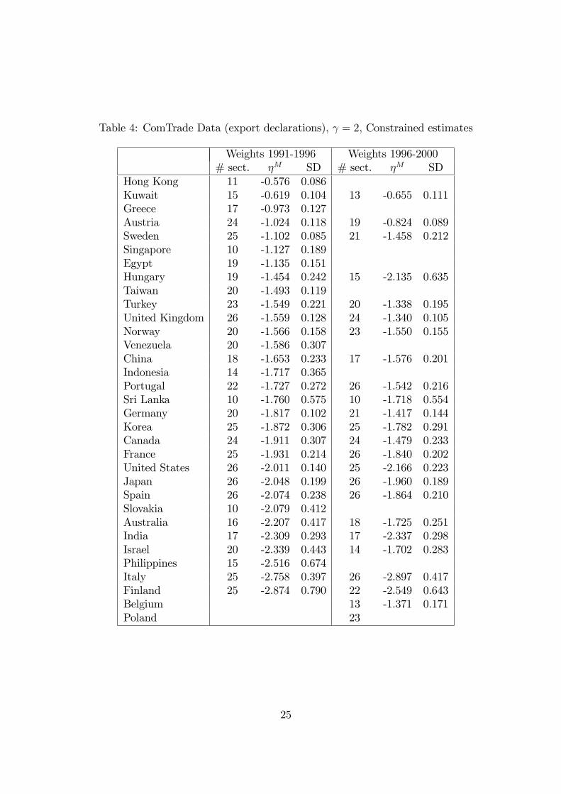
Table 4: ComTrade Data (export declarations), = 2, Constrained estimates

Weights 1991-1996 Weights 1996-2000# sect. �M SD # sect. �M SD

Hong Kong 11 -0.576 0.086Kuwait 15 -0.619 0.104 13 -0.655 0.111Greece 17 -0.973 0.127Austria 24 -1.024 0.118 19 -0.824 0.089Sweden 25 -1.102 0.085 21 -1.458 0.212Singapore 10 -1.127 0.189Egypt 19 -1.135 0.151Hungary 19 -1.454 0.242 15 -2.135 0.635Taiwan 20 -1.493 0.119Turkey 23 -1.549 0.221 20 -1.338 0.195United Kingdom 26 -1.559 0.128 24 -1.340 0.105Norway 20 -1.566 0.158 23 -1.550 0.155Venezuela 20 -1.586 0.307China 18 -1.653 0.233 17 -1.576 0.201Indonesia 14 -1.717 0.365Portugal 22 -1.727 0.272 26 -1.542 0.216Sri Lanka 10 -1.760 0.575 10 -1.718 0.554Germany 20 -1.817 0.102 21 -1.417 0.144Korea 25 -1.872 0.306 25 -1.782 0.291Canada 24 -1.911 0.307 24 -1.479 0.233France 25 -1.931 0.214 26 -1.840 0.202United States 26 -2.011 0.140 25 -2.166 0.223Japan 26 -2.048 0.199 26 -1.960 0.189Spain 26 -2.074 0.238 26 -1.864 0.210Slovakia 10 -2.079 0.412Australia 16 -2.207 0.417 18 -1.725 0.251India 17 -2.309 0.293 17 -2.337 0.298Israel 20 -2.339 0.443 14 -1.702 0.283Philippines 15 -2.516 0.674Italy 25 -2.758 0.397 26 -2.897 0.417Finland 25 -2.874 0.790 22 -2.549 0.643Belgium 13 -1.371 0.171Poland 23

25

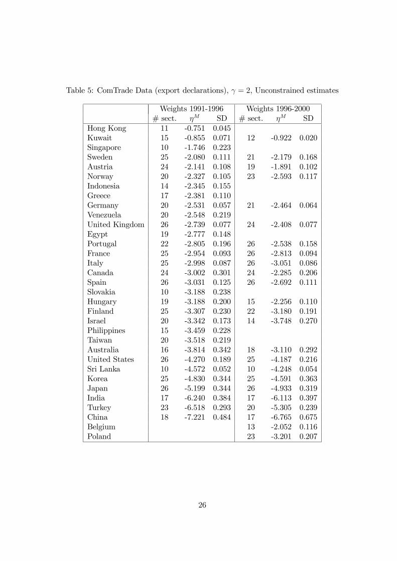
Table 5: ComTrade Data (export declarations), = 2, Unconstrained estimates

Weights 1991-1996 Weights 1996-2000# sect. �M SD # sect. �M SD

Hong Kong 11 -0.751 0.045Kuwait 15 -0.855 0.071 12 -0.922 0.020Singapore 10 -1.746 0.223Sweden 25 -2.080 0.111 21 -2.179 0.168Austria 24 -2.141 0.108 19 -1.891 0.102Norway 20 -2.327 0.105 23 -2.593 0.117Indonesia 14 -2.345 0.155Greece 17 -2.381 0.110Germany 20 -2.531 0.057 21 -2.464 0.064Venezuela 20 -2.548 0.219United Kingdom 26 -2.739 0.077 24 -2.408 0.077Egypt 19 -2.777 0.148Portugal 22 -2.805 0.196 26 -2.538 0.158France 25 -2.954 0.093 26 -2.813 0.094Italy 25 -2.998 0.087 26 -3.051 0.086Canada 24 -3.002 0.301 24 -2.285 0.206Spain 26 -3.031 0.125 26 -2.692 0.111Slovakia 10 -3.188 0.238Hungary 19 -3.188 0.200 15 -2.256 0.110Finland 25 -3.307 0.230 22 -3.180 0.191Israel 20 -3.342 0.173 14 -3.748 0.270Philippines 15 -3.459 0.228Taiwan 20 -3.518 0.219Australia 16 -3.814 0.342 18 -3.110 0.292United States 26 -4.270 0.189 25 -4.187 0.216Sri Lanka 10 -4.572 0.052 10 -4.248 0.054Korea 25 -4.830 0.344 25 -4.591 0.363Japan 26 -5.199 0.344 26 -4.933 0.319India 17 -6.240 0.384 17 -6.113 0.397Turkey 23 -6.518 0.293 20 -5.305 0.239China 18 -7.221 0.484 17 -6.765 0.675Belgium 13 -2.052 0.116Poland 23 -3.201 0.207

26

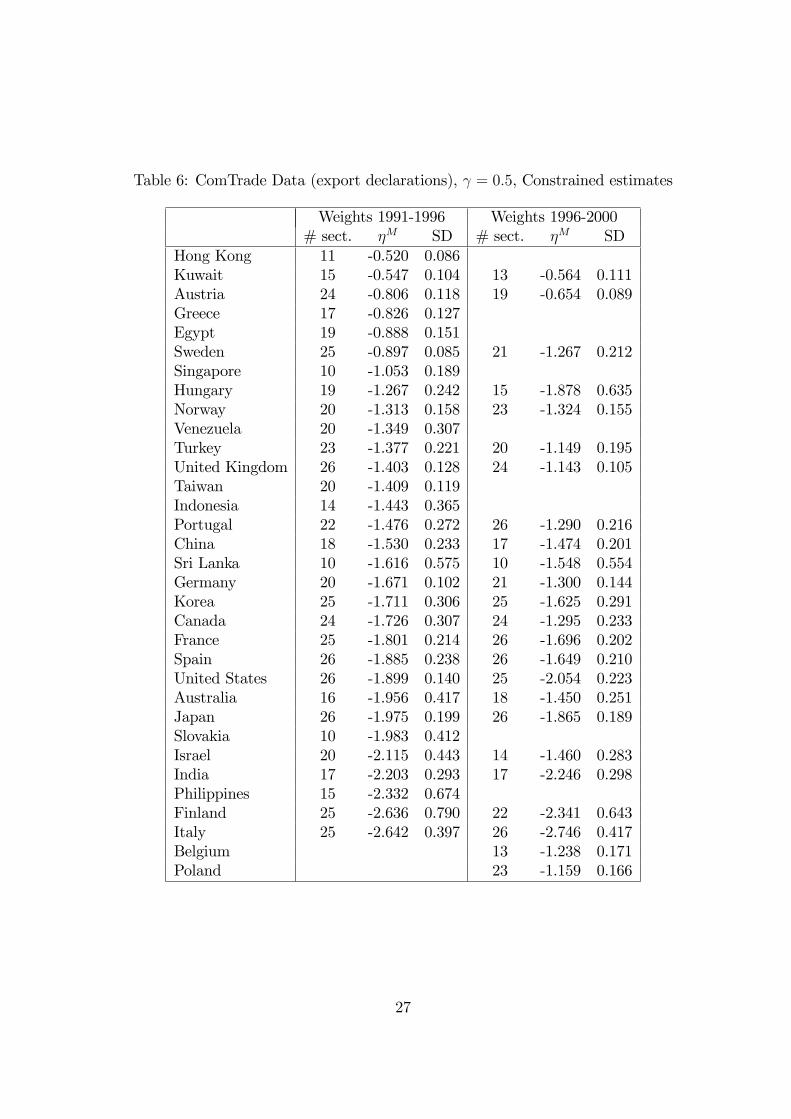
Table 6: ComTrade Data (export declarations), = 0:5, Constrained estimates

Weights 1991-1996 Weights 1996-2000# sect. �M SD # sect. �M SD

Hong Kong 11 -0.520 0.086Kuwait 15 -0.547 0.104 13 -0.564 0.111Austria 24 -0.806 0.118 19 -0.654 0.089Greece 17 -0.826 0.127Egypt 19 -0.888 0.151Sweden 25 -0.897 0.085 21 -1.267 0.212Singapore 10 -1.053 0.189Hungary 19 -1.267 0.242 15 -1.878 0.635Norway 20 -1.313 0.158 23 -1.324 0.155Venezuela 20 -1.349 0.307Turkey 23 -1.377 0.221 20 -1.149 0.195United Kingdom 26 -1.403 0.128 24 -1.143 0.105Taiwan 20 -1.409 0.119Indonesia 14 -1.443 0.365Portugal 22 -1.476 0.272 26 -1.290 0.216China 18 -1.530 0.233 17 -1.474 0.201Sri Lanka 10 -1.616 0.575 10 -1.548 0.554Germany 20 -1.671 0.102 21 -1.300 0.144Korea 25 -1.711 0.306 25 -1.625 0.291Canada 24 -1.726 0.307 24 -1.295 0.233France 25 -1.801 0.214 26 -1.696 0.202Spain 26 -1.885 0.238 26 -1.649 0.210United States 26 -1.899 0.140 25 -2.054 0.223Australia 16 -1.956 0.417 18 -1.450 0.251Japan 26 -1.975 0.199 26 -1.865 0.189Slovakia 10 -1.983 0.412Israel 20 -2.115 0.443 14 -1.460 0.283India 17 -2.203 0.293 17 -2.246 0.298Philippines 15 -2.332 0.674Finland 25 -2.636 0.790 22 -2.341 0.643Italy 25 -2.642 0.397 26 -2.746 0.417Belgium 13 -1.238 0.171Poland 23 -1.159 0.166

27

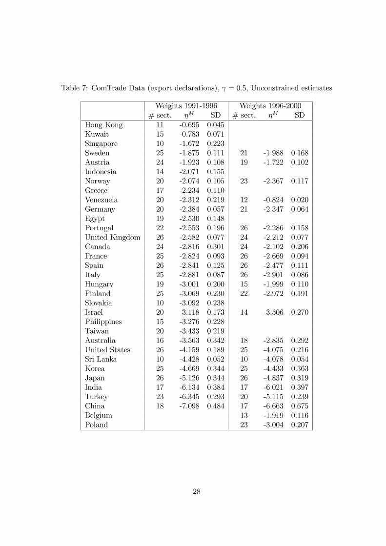
Table 7: ComTrade Data (export declarations), = 0:5, Unconstrained estimates

Weights 1991-1996 Weights 1996-2000# sect. �M SD # sect. �M SD

Hong Kong 11 -0.695 0.045Kuwait 15 -0.783 0.071Singapore 10 -1.672 0.223Sweden 25 -1.875 0.111 21 -1.988 0.168Austria 24 -1.923 0.108 19 -1.722 0.102Indonesia 14 -2.071 0.155Norway 20 -2.074 0.105 23 -2.367 0.117Greece 17 -2.234 0.110Venezuela 20 -2.312 0.219 12 -0.824 0.020Germany 20 -2.384 0.057 21 -2.347 0.064Egypt 19 -2.530 0.148Portugal 22 -2.553 0.196 26 -2.286 0.158United Kingdom 26 -2.582 0.077 24 -2.212 0.077Canada 24 -2.816 0.301 24 -2.102 0.206France 25 -2.824 0.093 26 -2.669 0.094Spain 26 -2.841 0.125 26 -2.477 0.111Italy 25 -2.881 0.087 26 -2.901 0.086Hungary 19 -3.001 0.200 15 -1.999 0.110Finland 25 -3.069 0.230 22 -2.972 0.191Slovakia 10 -3.092 0.238Israel 20 -3.118 0.173 14 -3.506 0.270Philippines 15 -3.276 0.228Taiwan 20 -3.433 0.219Australia 16 -3.563 0.342 18 -2.835 0.292United States 26 -4.159 0.189 25 -4.075 0.216Sri Lanka 10 -4.428 0.052 10 -4.078 0.054Korea 25 -4.669 0.344 25 -4.433 0.363Japan 26 -5.126 0.344 26 -4.837 0.319India 17 -6.134 0.384 17 -6.021 0.397Turkey 23 -6.345 0.293 20 -5.115 0.239China 18 -7.098 0.484 17 -6.663 0.675Belgium 13 -1.919 0.116Poland 23 -3.004 0.207

28

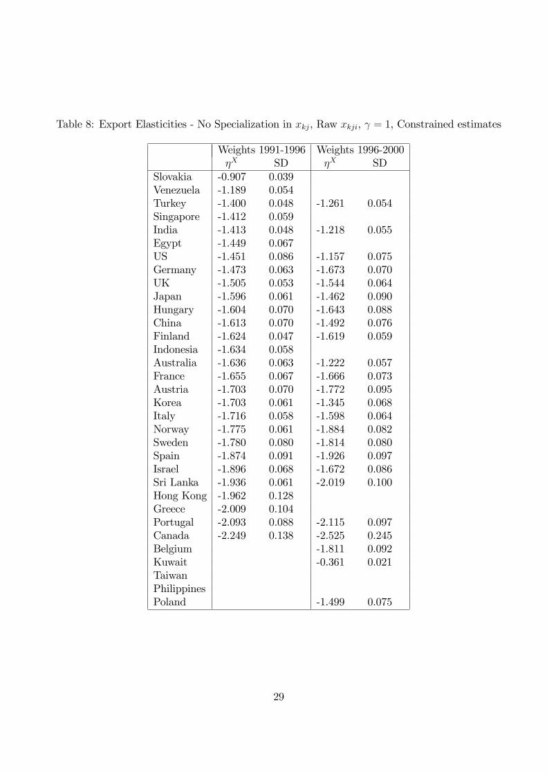
Table 8: Export Elasticities - No Specialization in xkj, Raw xkji, = 1, Constrained estimates

Weights 1991-1996 Weights 1996-2000�X SD �X SD

Slovakia -0.907 0.039Venezuela -1.189 0.054Turkey -1.400 0.048 -1.261 0.054Singapore -1.412 0.059India -1.413 0.048 -1.218 0.055Egypt -1.449 0.067US -1.451 0.086 -1.157 0.075Germany -1.473 0.063 -1.673 0.070UK -1.505 0.053 -1.544 0.064Japan -1.596 0.061 -1.462 0.090Hungary -1.604 0.070 -1.643 0.088China -1.613 0.070 -1.492 0.076Finland -1.624 0.047 -1.619 0.059Indonesia -1.634 0.058Australia -1.636 0.063 -1.222 0.057France -1.655 0.067 -1.666 0.073Austria -1.703 0.070 -1.772 0.095Korea -1.703 0.061 -1.345 0.068Italy -1.716 0.058 -1.598 0.064Norway -1.775 0.061 -1.884 0.082Sweden -1.780 0.080 -1.814 0.080Spain -1.874 0.091 -1.926 0.097Israel -1.896 0.068 -1.672 0.086Sri Lanka -1.936 0.061 -2.019 0.100Hong Kong -1.962 0.128Greece -2.009 0.104Portugal -2.093 0.088 -2.115 0.097Canada -2.249 0.138 -2.525 0.245Belgium -1.811 0.092Kuwait -0.361 0.021TaiwanPhilippinesPoland -1.499 0.075

29

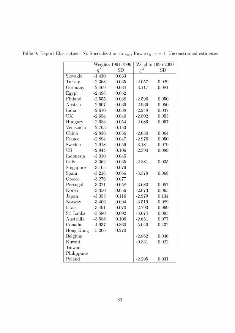
Table 9: Export Elasticities - No Specialization in xkj, Raw xkji, = 1, Unconstrained estimates

Weights 1991-1996 Weights 1996-2000�X SD �X SD

Slovakia -1.430 0.033Turkey -2.368 0.035 -2.057 0.029Germany -2.469 0.034 -3.117 0.081Egypt -2.496 0.052Finland -2.555 0.038 -2.596 0.050Austria -2.607 0.036 -2.936 0.050India -2.610 0.038 -2.248 0.037UK -2.654 0.040 -2.802 0.053Hungary -2.683 0.054 -2.686 0.057Venezuela -2.763 0.153China -2.836 0.056 -2.680 0.064France -2.894 0.047 -2.976 0.050Sweden -2.918 0.056 -3.181 0.079US -2.944 0.106 -2.390 0.089Indonesia -3.010 0.045Italy -3.062 0.035 -2.881 0.035Singapore -3.105 0.079Spain -3.216 0.066 -3.378 0.068Greece -3.276 0.077Portugal -3.321 0.058 -3.680 0.057Korea -3.350 0.056 -2.673 0.065Japan -3.355 0.116 -2.979 0.134Norway -3.406 0.094 -3.519 0.089Israel -3.491 0.070 -2.793 0.069Sri Lanka -3.580 0.092 -3.674 0.095Australia -3.588 0.106 -2.651 0.077Canada -4.937 0.360 -5.046 0.432Hong Kong -5.206 0.270Belgium -2.862 0.046Kuwait -0.831 0.022TaiwanPhilippinesPoland -2.295 0.031

30

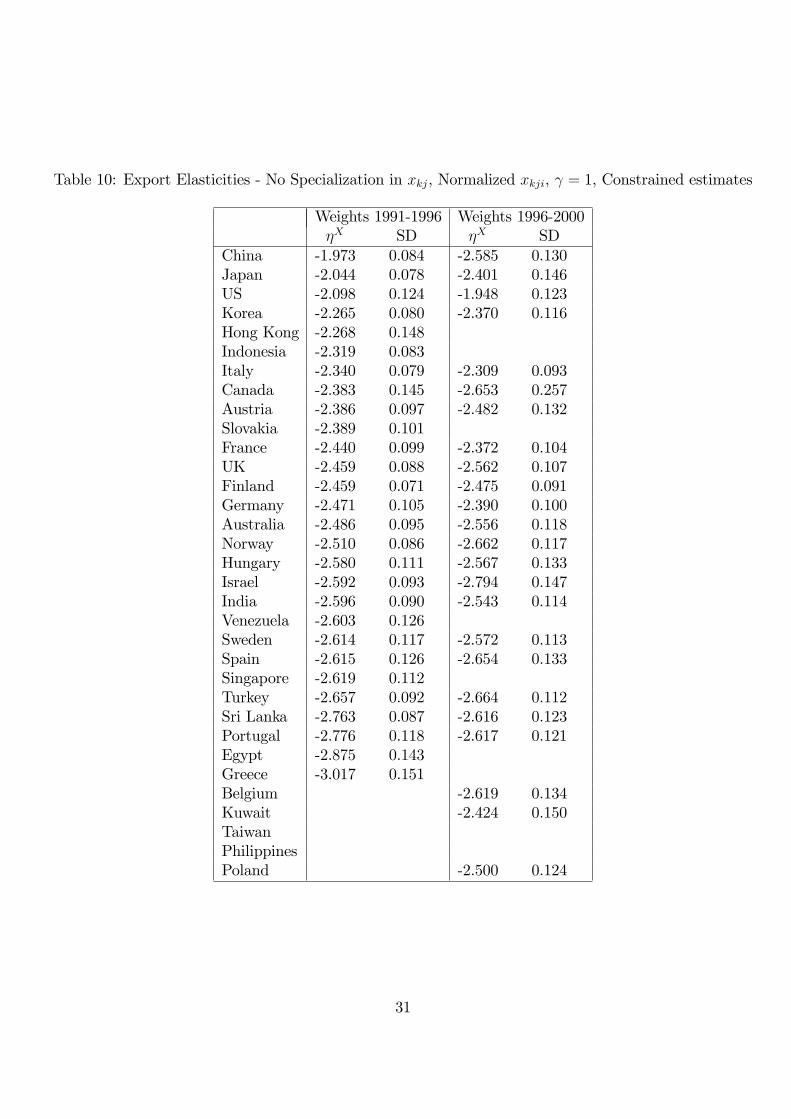
Table 10: Export Elasticities - No Specialization in xkj, Normalized xkji, = 1, Constrained estimates

Weights 1991-1996 Weights 1996-2000�X SD �X SD

China -1.973 0.084 -2.585 0.130Japan -2.044 0.078 -2.401 0.146US -2.098 0.124 -1.948 0.123Korea -2.265 0.080 -2.370 0.116Hong Kong -2.268 0.148Indonesia -2.319 0.083Italy -2.340 0.079 -2.309 0.093Canada -2.383 0.145 -2.653 0.257Austria -2.386 0.097 -2.482 0.132Slovakia -2.389 0.101France -2.440 0.099 -2.372 0.104UK -2.459 0.088 -2.562 0.107Finland -2.459 0.071 -2.475 0.091Germany -2.471 0.105 -2.390 0.100Australia -2.486 0.095 -2.556 0.118Norway -2.510 0.086 -2.662 0.117Hungary -2.580 0.111 -2.567 0.133Israel -2.592 0.093 -2.794 0.147India -2.596 0.090 -2.543 0.114Venezuela -2.603 0.126Sweden -2.614 0.117 -2.572 0.113Spain -2.615 0.126 -2.654 0.133Singapore -2.619 0.112Turkey -2.657 0.092 -2.664 0.112Sri Lanka -2.763 0.087 -2.616 0.123Portugal -2.776 0.118 -2.617 0.121Egypt -2.875 0.143Greece -3.017 0.151Belgium -2.619 0.134Kuwait -2.424 0.150TaiwanPhilippinesPoland -2.500 0.124

31

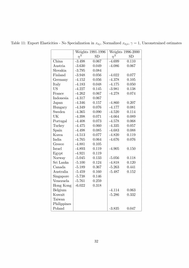
Table 11: Export Elasticities - No Specialization in xkj, Normalized xkji, = 1, Unconstrained estimates

Weights 1991-1996 Weights 1996-2000�X SD �X SD

China -3.498 0.067 -4.699 0.110Austria -3.630 0.049 -4.086 0.067Slovakia -3.795 0.084Finland -3.948 0.056 -4.022 0.077Germany -4.152 0.056 -4.378 0.105Italy -4.183 0.048 -4.175 0.050US -4.227 0.145 -3.981 0.138France -4.262 0.067 -4.278 0.074Indonesia -4.317 0.067Japan -4.346 0.157 -4.860 0.207Hungary -4.349 0.076 -4.177 0.081Sweden -4.365 0.090 -4.520 0.114UK -4.398 0.071 -4.664 0.089Portugal -4.408 0.073 -4.578 0.068Turkey -4.475 0.060 -4.335 0.057Spain -4.498 0.085 -4.683 0.088Korea -4.513 0.077 -4.820 0.119India -4.765 0.064 -4.676 0.076Greece -4.881 0.105Israel -4.893 0.119 -4.905 0.150Egypt -4.921 0.119Norway -5.045 0.133 -5.056 0.118Sri Lanka -5.100 0.124 -4.818 0.120Canada -5.189 0.367 -5.263 0.441Australia -5.459 0.160 -5.487 0.152Singapore -5.738 0.146Venezuela -5.761 0.259Hong Kong -6.022 0.318Belgium -4.114 0.063Kuwait -5.286 0.332TaiwanPhilippinesPoland -3.835 0.047

32

Table 12: Export Elasticities - Specialization in xkj, Raw xkji, = 1, Constrained estimates

Weights 1991-1996 Weights 1996-2000�X SD �X SD

Slovakia -1.020 0.045Venezuela -1.216 0.068Singapore -1.264 0.044Australia -1.380 0.056 -1.017 0.048Egypt -1.446 0.060India -1.467 0.047 -1.315 0.065United States -1.477 0.088 -1.178 0.077Turkey -1.512 0.051 -1.352 0.058Germany -1.518 0.064 -1.629 0.068United Kingdom -1.542 0.055 -1.541 0.064China -1.554 0.065 -1.403 0.072Finland -1.573 0.045 -1.647 0.062Japan -1.602 0.061 -1.472 0.091Hungary -1.638 0.068 -1.782 0.094France -1.663 0.068 -1.679 0.074Korea -1.672 0.059 -1.291 0.063Austria -1.674 0.067 -1.752 0.094Italy -1.688 0.057 -1.613 0.065Indonesia -1.692 0.060Hong Kong -1.748 0.083Israel -1.782 0.069 -1.828 0.112Sweden -1.788 0.081 -1.799 0.083Norway -1.793 0.064 -1.791 0.075Spain -1.878 0.092 -1.918 0.096Greece -1.888 0.086Sri Lanka -1.984 0.075 -2.256 0.152Portugal -2.090 0.084 -2.073 0.092Canada -2.238 0.136 -2.518 0.243Belgium -1.790 0.083Kuwait -0.239 0.014TaiwanPhilippinesPoland -1.572 0.082

33

Table 13: Export Elasticities - Specialization in xkj, Raw xkji, = 1, Unconstrained estimates

Weights 1991-1996 Weights 1996-2000�X SD �X SD

Slovakia -1.658 0.025Singapore -2.414 0.040Egypt -2.454 0.047Finland -2.592 0.039 -2.766 0.055Austria -2.593 0.036 -2.915 0.048India -2.634 0.035 -2.309 0.034United Kingdom -2.671 0.038 -2.756 0.049Turkey -2.702 0.044 -2.410 0.035Germany -2.768 0.054 -3.002 0.070France -2.879 0.044 -3.000 0.051China -2.893 0.053 -2.608 0.044Israel -2.909 0.045 -2.734 0.042Hungary -2.940 0.052 -3.351 0.070Sweden -2.990 0.062 -3.151 0.065United States -3.025 0.111 -2.452 0.094Italy -3.053 0.036 -2.953 0.038Australia -3.116 0.113 -2.344 0.083Greece -3.236 0.052Spain -3.264 0.069 -3.415 0.070Korea -3.374 0.059 -2.650 0.066Japan -3.385 0.121 -3.036 0.145Indonesia -3.435 0.125Norway -3.484 0.072 -3.445 0.070Portugal -3.680 0.066 -3.718 0.067Sri Lanka -3.774 0.086 -4.241 0.159Hong Kong -4.360 0.183Canada -5.291 0.334 -5.485 0.411Venezuela -6.671 0.070Belgium -3.056 0.043Kuwait -0.538 0.024TaiwanPhilippinesPoland -2.574 0.038

34

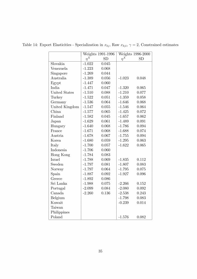
Table 14: Export Elasticities - Specialization in xkj, Raw xkji, = 2, Constrained estimates

Weights 1991-1996 Weights 1996-2000�X SD �X SD

Slovakia -1.022 0.045Venezuela -1.223 0.068Singapore -1.269 0.044Australia -1.389 0.056 -1.023 0.048Egypt -1.447 0.060India -1.471 0.047 -1.320 0.065United States -1.510 0.088 -1.210 0.077Turkey -1.522 0.051 -1.359 0.058Germany -1.536 0.064 -1.646 0.068United Kingdom -1.547 0.055 -1.546 0.064China -1.577 0.065 -1.425 0.072Finland -1.582 0.045 -1.657 0.062Japan -1.629 0.061 -1.489 0.091Hungary -1.640 0.068 -1.786 0.094France -1.671 0.068 -1.688 0.074Austria -1.678 0.067 -1.755 0.094Korea -1.680 0.059 -1.295 0.063Italy -1.700 0.057 -1.622 0.065Indonesia -1.706 0.060Hong Kong -1.784 0.083Israel -1.788 0.069 -1.835 0.112Sweden -1.797 0.081 -1.807 0.083Norway -1.797 0.064 -1.795 0.075Spain -1.887 0.092 -1.927 0.096Greece -1.892 0.086Sri Lanka -1.988 0.075 -2.266 0.152Portugal -2.099 0.084 -2.080 0.092Canada -2.260 0.136 -2.538 0.243Belgium -1.798 0.083Kuwait -0.239 0.014TaiwanPhilippinesPoland -1.576 0.082

35

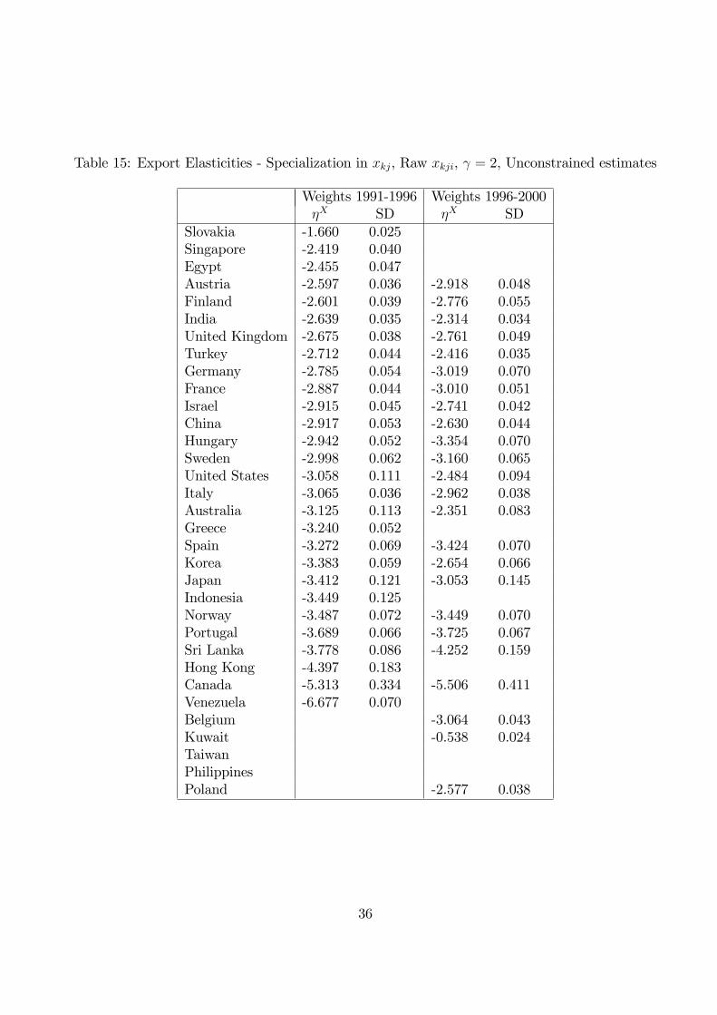
Table 15: Export Elasticities - Specialization in xkj, Raw xkji, = 2, Unconstrained estimates

Weights 1991-1996 Weights 1996-2000�X SD �X SD

Slovakia -1.660 0.025Singapore -2.419 0.040Egypt -2.455 0.047Austria -2.597 0.036 -2.918 0.048Finland -2.601 0.039 -2.776 0.055India -2.639 0.035 -2.314 0.034United Kingdom -2.675 0.038 -2.761 0.049Turkey -2.712 0.044 -2.416 0.035Germany -2.785 0.054 -3.019 0.070France -2.887 0.044 -3.010 0.051Israel -2.915 0.045 -2.741 0.042China -2.917 0.053 -2.630 0.044Hungary -2.942 0.052 -3.354 0.070Sweden -2.998 0.062 -3.160 0.065United States -3.058 0.111 -2.484 0.094Italy -3.065 0.036 -2.962 0.038Australia -3.125 0.113 -2.351 0.083Greece -3.240 0.052Spain -3.272 0.069 -3.424 0.070Korea -3.383 0.059 -2.654 0.066Japan -3.412 0.121 -3.053 0.145Indonesia -3.449 0.125Norway -3.487 0.072 -3.449 0.070Portugal -3.689 0.066 -3.725 0.067Sri Lanka -3.778 0.086 -4.252 0.159Hong Kong -4.397 0.183Canada -5.313 0.334 -5.506 0.411Venezuela -6.677 0.070Belgium -3.064 0.043Kuwait -0.538 0.024TaiwanPhilippinesPoland -2.577 0.038

36

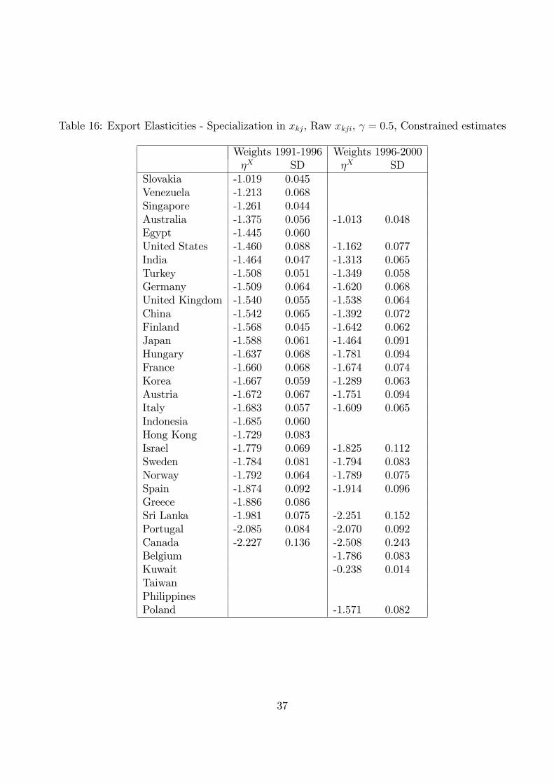
Table 16: Export Elasticities - Specialization in xkj, Raw xkji, = 0:5, Constrained estimates

Weights 1991-1996 Weights 1996-2000�X SD �X SD

Slovakia -1.019 0.045Venezuela -1.213 0.068Singapore -1.261 0.044Australia -1.375 0.056 -1.013 0.048Egypt -1.445 0.060United States -1.460 0.088 -1.162 0.077India -1.464 0.047 -1.313 0.065Turkey -1.508 0.051 -1.349 0.058Germany -1.509 0.064 -1.620 0.068United Kingdom -1.540 0.055 -1.538 0.064China -1.542 0.065 -1.392 0.072Finland -1.568 0.045 -1.642 0.062Japan -1.588 0.061 -1.464 0.091Hungary -1.637 0.068 -1.781 0.094France -1.660 0.068 -1.674 0.074Korea -1.667 0.059 -1.289 0.063Austria -1.672 0.067 -1.751 0.094Italy -1.683 0.057 -1.609 0.065Indonesia -1.685 0.060Hong Kong -1.729 0.083Israel -1.779 0.069 -1.825 0.112Sweden -1.784 0.081 -1.794 0.083Norway -1.792 0.064 -1.789 0.075Spain -1.874 0.092 -1.914 0.096Greece -1.886 0.086Sri Lanka -1.981 0.075 -2.251 0.152Portugal -2.085 0.084 -2.070 0.092Canada -2.227 0.136 -2.508 0.243Belgium -1.786 0.083Kuwait -0.238 0.014TaiwanPhilippinesPoland -1.571 0.082

37

Table 17: Export Elasticities - Specialization in xkj, Raw xkji, = 0:5, Unconstrained estimates

Weights 1991-1996 Weights 1996-2000�X SD �X SD

Slovakia -1.657 0.025Singapore -2.411 0.040Egypt -2.453 0.047Finland -2.587 0.039 -2.761 0.055Austria -2.591 0.036 -2.913 0.048India -2.632 0.035 -2.306 0.034United Kingdom -2.668 0.038 -2.754 0.049Turkey -2.698 0.044 -2.406 0.035Germany -2.759 0.054 -2.994 0.070France -2.875 0.044 -2.996 0.051China -2.882 0.053 -2.596 0.044Israel -2.905 0.045 -2.730 0.042Hungary -2.939 0.052 -3.349 0.070Sweden -2.986 0.062 -3.147 0.065United States -3.008 0.111 -2.436 0.094Italy -3.047 0.036 -2.948 0.038Australia -3.111 0.113 -2.341 0.083Greece -3.234 0.052Spain -3.260 0.069 -3.411 0.070Korea -3.370 0.059 -2.648 0.066Japan -3.371 0.121 -3.028 0.145Indonesia -3.428 0.125Norway -3.482 0.072 -3.443 0.070Portugal -3.675 0.066 -3.715 0.067Sri Lanka -3.772 0.086 -4.236 0.159Hong Kong -4.342 0.183Canada -5.280 0.334 -5.475 0.411Venezuela -6.667 0.070Belgium -3.052 0.043Kuwait -0.538 0.024TaiwanPhilippinesPoland -2.573 0.038

38