Trade Facilitation and the Extensive Margin-Finalcid.econ.ucdavis.edu/Papers/Trade_Facilitation_and_the_Extensive... · Trade Facilitation and the Extensive Margin of Exports Robert

Forthcoming, Japanese Economic Review

Trade Facilitation and the Extensive Margin of Exports

Robert C. Feenstra, University of California - Davis and NBER

Hong Ma, Tsinghua University

December 2013

Abstract

This paper examines the link between trade facilitation and export variety for a broad cross-

section of countries. We measure trade facilitation using port efficiency. We also include the

bilateral import tariff and OECD membership and regional trade agreement. We find that port

efficiency contributes significantly to the extensive margin of exports, and that the bilateral

import tariff negatively impacts variety of exports. The positive effect is confirmed when

examining trade between countries without common land border, or between OECD member

countries and non-OECD countries. Results are not as strong when we look at within-OECD

trade, or focus on bilateral trade in the intensive margin.

JEL code: F13， F14

Address for correspondence: Hong Ma, Department of Economics, Tsinghua University, Beijing, 100086, China. [email protected]. Tel: (86)-10-62794388. Fax: (86)-10-62785562.

2

1. Introduction

Recent literature in international trade has emphasized the extensive margin, by which we

mean the variety that a country exports and imports. When a country imports more varieties then

its consumers gain, as has been shown empirically for the United States by Broda and Weinstein

(2006). But as a country exports more product varieties then its producers also gain, as has been

shown by Feenstra and Kee (2008). This gain arises due to improved productivity in a model

with heterogeneous firms, due to Melitz (2003). When a country faces improved market

opportunities abroad the high-productivity firms will begin to export. The entry of those firms

will drive up factor prices in the sector and force out lower-productivity domestic firms. So

improved market opportunities abroad are associated with greater product variety of exports and

higher overall productivity in a sector.

This linkage between export variety and productivity raises a potential for welfare-

enhancing government policies via trade facilitation. Within this broad category of policies we

include actions that allow for enhanced exports, through infrastructure development, foreign

marketing opportunities, institutions, etc1. The logic of the Melitz model is that such actions that

facilitate trade will raise export variety and average productivity. There has been a rapidly-

growing body of literature discussing various actions that promote or facilitate trade flow across

countries. Recent research by Limao and Venables (2000) has shown that a 10 percent decrease

in transport cost raises trade volume by more than 20 percent. The reduction in transport costs

could be due to improvement in infrastructure, for example, the improvement in ocean ports

facilities. Clark, Dollar and Micco (2004) analyze the effect of port efficiency on bilateral trade

flows and shows that improving port efficiency does reduce shipping costs a lot. Finally, a series

1 In the WTO, trade facilitation is defined as “the simplification and harmonization of international trade procedures” covering the “activities, practices and formalities involved in collecting, presenting, communicating and processing data required for the movement of goods in international trade”.

3

of World Bank working papers has empirically explored the trade-facilitating impact of

standards (Chen et al. 2008), road network quality (Shepherd and Wilson, 2006), and other

factors such as port efficiency, custom regimes, regulatory policy and technology, etc. (Wilson,

Mann and Otsuki, 2005; Soloaga, et al. 2006).

With few exceptions, most of current works focus on the effect of trade facilitation on

trade flows, instead of on the extensive margin or export variety. One exception is Kehoe and

Ruhl (2004), who show that trade liberalization such as NAFTA drives growth in the extensive

margin, which is an important source of new trade. A closely related literature has studied the

impact of currency union. For example, Baldwin and Di Nino (2006) examine the effect of the

Euro on the extensive margin of trade among European countries. While Bergin and Lin (2009)

use the NBER-UN world trade dataset to study the different effects of exchange rate regimes on

the extensive and intensive margins. Furthermore, research emphasizing the export

diversification of developing countries naturally relates itself to studies of the export variety and

its determinants. For example, Dennis and Shepherd (2007) and Amurgo-Pacheco and Pierola

(2008) both focus on patterns of trade diversification in developing countries. In short, there is an

emerging attention on the cross-border trade in varieties, instead of in volume.

In this paper, we examine the link between trade facilitation and export variety for a

broad cross-section of countries over 13 years (1991-2003). We measure trade facilitation using

the data on the efficiency of ports, from Blonigen and Wilson (2008). The extensive margin of

exports is constructed as in Hummels and Klenow (2005), but allowing both cross-sectional and

time-series variations. We also include other variables that can impact trade in our specification;

notably, the trade restrictiveness index due to Kee et al (2009), as well as institutional variables

such as Regional Trade Agreement.

4

This paper first adopts the Feenstra (1994) method to develop a panel of bilateral export

variety measure, as discussed in section 2. This has been developed for a cross-section sample by

Hummels and Klenow (2005), where export variety is named the “extensive margin” of exports.

Following Feenstra and Kee (2008), we define the export variety (or extensive margin of

exports) of country h to country j as the worldwide average export over all years to country j in

those categories where country h actually exports to j, relative to the worldwide average export

to j over all years in all categories. By this method, our measure of export variety is consistent

both across countries and over time, as discussed in section 3.

We then adopt a conventional empirical method, the gravity regression, to estimate

how the export variety between two countries is influenced by ocean port efficiency, bilateral

trade tariff, international institutions such as OECD, Regional Trade Agreement, etc. It is

important to single out export variety for empirical investigation and to understand the role and

the determinants of the extensive margins of trade. Conventional gravity equation using total

trade flows as dependent variable, though armed with the micro-foundation provided in

Anderson and van Wincoop (2003), might be misguiding since the extensive margin and the

intensive margin might correspond differently to trade costs and trade facilitation factors. As

revealed in Bernard, et al. (2007), the extensive margins of trade are central to understand the

effect of trade costs on trade flows. In fact, following a method proposed in Eaton, Kortum and

Kramarz (2004), Bernard, et al. (2007) decompose export flow into three components: the

number of firms exporting to a destination, the number of products exported to that destination,

and average exports per product per firm. Separately regressing each component on the usual

gravity variables such as distance and income, they find that it is the first two items --- the

extensive margin --- that explains the dampening effect of distance, while the average export

5

value --- the intensive margin --- is increasing in distance. This is in sharp contrast to the

conventional belief that distance or trade cost reduces aggregate and average trade flow

(assuming all firms export), and this also motivates our investigation in this paper on the

different effects of port efficiency on the extensive and intensive margins. Finally, there are a

few papers attempting to explain the theoretical reason why the extensive margin and the

intensive margin adjust differently with respect to trade costs. One example is Bergin and Lin

(2009). They construct a stochastic general equilibrium model, assuming sticky prices and fixed

costs of entry, to explain the different effect of exchange rate uncertainty on the extensive margin

(firm number) and the intensive margin (average value).

Section 4 summarizes our data, and section 5 presents the estimation. In our

benchmark regression we find that bilateral port efficiency has a significant and positive impact

on export variety (i.e., the extensive margin). The impact on export volume (i.e., the intensive

margin) is positive, but not significant. A 10 percent improvement in the bilateral port efficiency

increases export variety by 1.5 to 3.4 percent, while it can only increase the intensive margin of

export by 0.2 to 1.0 percent. Port efficiency appears to matter much more for the extensive

margin rather than for the intensive margin.

Similarly, for trade barriers, we look at the simple average of bilateral import tariff. Not

surprisingly, tariff appears to discourage expansion in export variety, but it only has insignificant

impact on the intensive margin. Furthermore, sharing the same language seems to promote trade

at both the extensive and intensive margins. Regional Trade Agreement and sharing common

land border both promote export volume, while the former discourages export of variety.

Interestingly, being an OECD member for importing countries is shown to promote the range of

6

export variety a great deal, while exporting countries’ OECD membership does not have

significant effect on export variety.

To further explore the impact of trade facilitation on export variety, we divide the sample

into 5 sub-groups, namely, trade among OECD countries, trade between member country and

non-member countries, and trade among non-OECD countries, and finally trade between

countries without common land border. Results are not as strong when we use only the OECD

countries, or focus on the intensive margin rather than variety, but continue to hold when at least

one trading nation is not OECD member, or when we exclude countries with contiguous border

with each other. We conclude in section 6.

2. Measuring New Varieties in International Trade

We start from Feenstra (1994), who shows how to construct an exact import price index

that accounts for both newly-created import varieties over time and taste or quality changes in

existing varieties. This exact price index can be derived from a non-symmetric CES utility

function. Consider home country h importing from many countries, each of which exports many

types of commodities. For simplicity we aggregate these goods into a single sector, but the

extension to multiple sectors will be immediate2. For each period t, let the set of goods

consumed in country h be denoted by ,....}.3,2,1{htI Then the quantity vector of each type of

goods consumed in country h in period t is denoted by 0htq . The representative consumer’s

preferences are characterized by a non-symmetric CES utility function, which is:

1 ,)(),()1/(/)1(

htIi

hitit

ht

ht

ht qaIqUU , (1)

2 See, for example, Broda and Weinstein (2006), for an aggregate exact price index derived from a composite CES function incorporating many sectors and many countries.

7

where denotes the elasticity of substitution among all varieties, which is assumed to exceed

unity; ait > 0 denotes a parameter measuring taste (or quality) for good i, which is allowed to

vary over time; and htI denotes the set of goods available in period t, at the prices 0h

itp .

By duality, the minimum unit-cost function is also a CES form:

itIi

hitit

ht

ht apbIpc h

t

it

)1/(11 b 1, ,)(),( . (2)

The CES unit-cost function specified above changes with evolving variety set htI , therefore it

cannot be evaluated without knowledge of the taste (or quality) parameter itb . However, a result

from index number theory is that the ratio of cost functions can be evaluated using data on prices

and qualities in the two periods or two countries. Our interest is in the ratio ),(

),(

11ht

ht

ht

ht

Ipc

Ipc

, which

can be measured as follows:

Proposition (Feenstra, 1994)

Assume that itit bb 1 for ht

ht

h IIIi 1 , and that the quantities are cost-minimizing.

Then for > 1:

)/(

ht

hthh

tht

ht

htSVhh

t

hht

)I(

)I()I,q,q,p,p(P

)I,p(c

)I,p(c11

111

1

(3)

where

h

hi

Ii

I

hit

hithh

tht

ht

htSV

p

pIqqppP

)(

1

11 ),,,,(

is the price index due to Sato (1977)

and Vartia (1977), constructed as a geometric mean of the price ratios with the weights )I( h

i ,

which are constructed from the expenditure shares as in (4) and (5),

hIi

hit

hit

hit

hith

it qp

qpIs )( (4)

8

)(ln–)(ln

)(–)(

)(ln–)(ln

)(–)()(

1

1

1

1

hIih

ith

it

hit

hit

hit

hit

hit

hith

i IsIs

IsIs

IsIs

IsIsI . (5)

and the values )( ht I and )(1

ht I are constructed as:

ttqp

qp

qp

qpI

h

hh

h

h

Ii ii

IiIi ii

Ii

hi

hi

Ii

hi

hih ,1,1)( ,

, (6)

This theorem states that the exact price index with variety change is equal to the Sato-Vartia PSV,

multiplied by a term of )/(ht

ht )]I(/)I([ 11

1

, which captures the creation and destruction

of varieties over time.

Notice that each of the terms 1)( hI can be interpreted as the period expenditure

on the varieties in the overlapping set hI , relative to the period total expenditure.

Alternatively, this can be interpreted as one minus the period expenditure on “new” varieties

(not in the set hI ), relative to the period total expenditure. When there is a greater number of

new varieties in period t, or more precisely, when the new varieties take greater share of

expenditure than disappearing varieties, the value of )( ht I will be lower than )I( h

t 1 . Then

the exact price index will be lower relative to the “conventional” price index which does not take

into account the change of varieties. Thus )( ht I provides an inverse measure of new varieties

in period t.

The term )/(ht

ht )]I(/)I([ 11

1

measures the decrease in unit-cost (or price index)

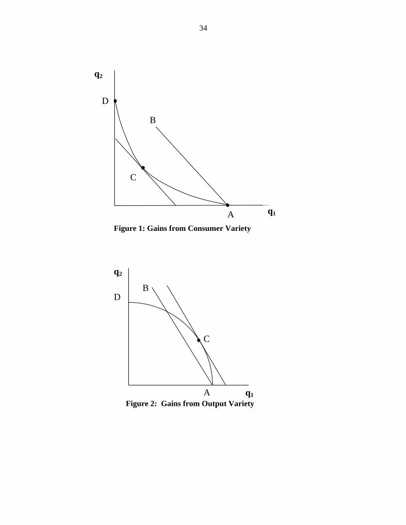
due to expansion of varieties range. Figure 1 illustrates the gains from adding a new variety. We

consider a two-goods case: when only one product ( 1q ) is available (at A), the minimum cost of

achieving the utility level U (represented by the indifference curve ACD) is the budget line AB.

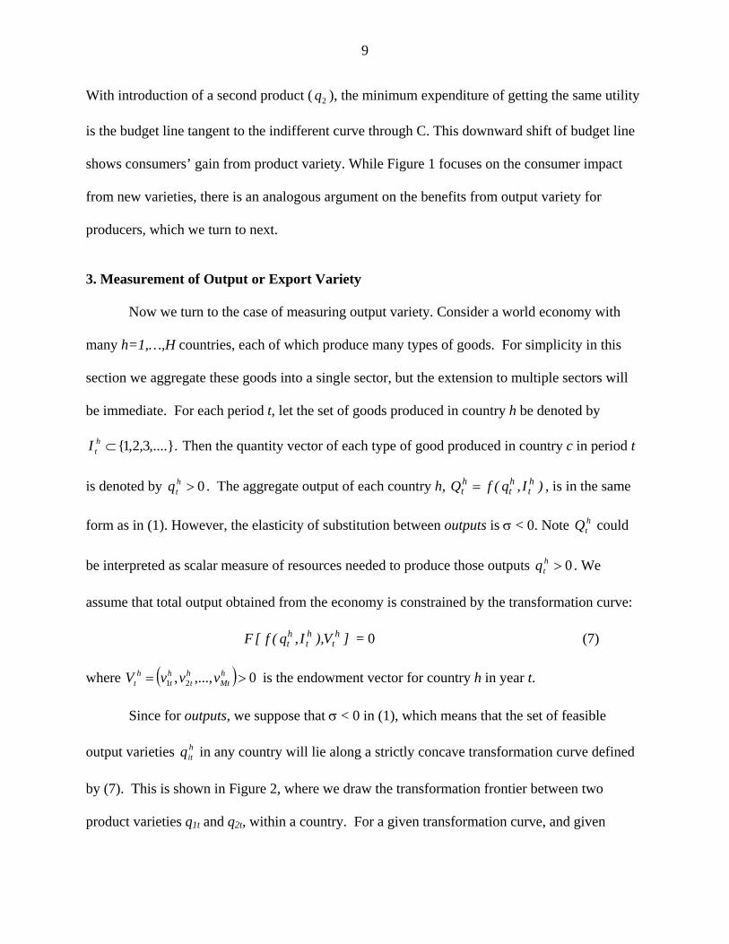
9

With introduction of a second product ( 2q ), the minimum expenditure of getting the same utility

is the budget line tangent to the indifferent curve through C. This downward shift of budget line

shows consumers’ gain from product variety. While Figure 1 focuses on the consumer impact

from new varieties, there is an analogous argument on the benefits from output variety for

producers, which we turn to next.

3. Measurement of Output or Export Variety

Now we turn to the case of measuring output variety. Consider a world economy with

many h=1,…,H countries, each of which produce many types of goods. For simplicity in this

section we aggregate these goods into a single sector, but the extension to multiple sectors will

be immediate. For each period t, let the set of goods produced in country h be denoted by

,....}.3,2,1{htI Then the quantity vector of each type of good produced in country c in period t

is denoted by 0htq . The aggregate output of each country h, )I,q(fQ h

tht

ht , is in the same

form as in (1). However, the elasticity of substitution between outputs is < 0. Note htQ could

be interpreted as scalar measure of resources needed to produce those outputs 0htq . We

assume that total output obtained from the economy is constrained by the transformation curve:

]V),I,q(f[F ht

ht

ht = 0 (7)

where 0,...,, 21 hMt

ht

ht

ht vvvV is the endowment vector for country h in year t.

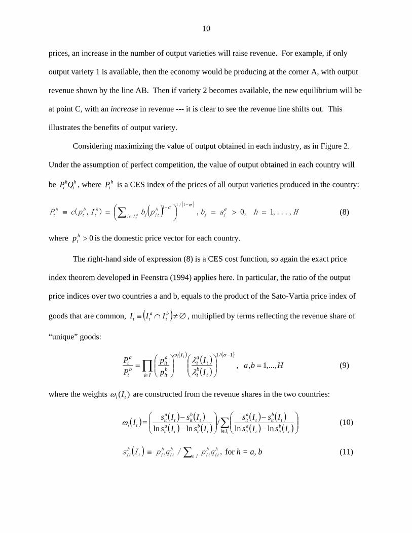
Since for outputs, we suppose that < 0 in (1), which means that the set of feasible

output varieties hitq in any country will lie along a strictly concave transformation curve defined

by (7). This is shown in Figure 2, where we draw the transformation frontier between two

product varieties q1t and q2t, within a country. For a given transformation curve, and given

10

prices, an increase in the number of output varieties will raise revenue. For example, if only

output variety 1 is available, then the economy would be producing at the corner A, with output

revenue shown by the line AB. Then if variety 2 becomes available, the new equilibrium will be

at point C, with an increase in revenue --- it is clear to see the revenue line shifts out. This

illustrates the benefits of output variety.

Considering maximizing the value of output obtained in each industry, as in Figure 2.

Under the assumption of perfect competition, the value of output obtained in each country will

be ht

ht QP , where h

tP is a CES index of the prices of all output varieties produced in the country:

HhabpbIpcP iiIi

hiti

ht

ht

ht h

t

,...,1,0,),(1/1

1

(8)

where 0htp is the domestic price vector for each country.

The right-hand side of expression (8) is a CES cost function, so again the exact price

index theorem developed in Feenstra (1994) applies here. In particular, the ratio of the output

price indices over two countries a and b, equals to the product of the Sato-Vartia price index of

goods that are common, bt

att III , multiplied by terms reflecting the revenue share of

“unique” goods:

H,...,b,a,I

I

p

p

P

P/

tbt

tat

I

Iibit

ait

bt

at

ti

1

11

(9)

where the weights )( ti I are constructed from the revenue shares in the two countries:

tIi t

bitt

ait

tbitt

ait

tbitt

ait

tbitt

ait

ti IsIs

IsIs

IsIs

IsIsI

lnln/

lnln (10)

,/

I

hit

hit

hit

hitt

hit qpqpIs for h = a, b (11)

11

,1 ,

ht

ht

ht Ii

hit

hit

IiIi

hit

hit

Ii

hit

hit

Ii

hit

hit

tht

qp

qp

qp

qpI for h = a, b. (12)

Notice that the output shares in (11), for each country, are measured relative to the common set

of goods tI . Then the weights in (10) are the logarithmic mean of the shares )( tait Is and )( t

bit Is ,

and sum to unity over the set of goods tIi .3

To interpret (12), notice that 1)( tht I due to the differing summations in the

numerator and denominator. This term will be strictly less than one if there are goods in the set

htI that are not found in the common set tI . In other words, if country a is selling some goods in

period t that are not sold by country b, this will make 1)( tat I . Then we could use

)(/)( tbtt

at II as an inverse measure of country a’s export variety, relative to country b. Having

more export variety in a ( i.e. having lower )(/)( tbtt

at II ) leads to a higher price index for a

(because 0 ), reflecting an increase in a’s revenue.

For cross-section comparison of tbtt

at I/I , we could choose the worldwide exports

to all destinations as a consistent “comparison country”. Let h

ht

wt II is the complete set of

varieties exported by the world in year t, and let wit

wit qp be the total value of imports for good i.

Then comparing country h to the world in year t, it is obvious that the common set is the goods

exported by h, i.e., bahIIII ht

wt

htt ,; . Therefore, bahI hh

t t,;1 , then a direct

measure of country h’s export variety (recall 0 ) is :

3 More precisely, the numerator of (10) is the logarithmic mean of the output shares of the two countries, and lies

in-between these shares. The denominator of (10) is introduced so that the weights )( ti I sum to unity.

12

bahqp

qpI

wt

ht

Ii

wit

wit

Ii

wit

with

twt ,,)(

(13)

The system (9)-(13) above is exactly a cross-country analogue to the time-series import

price index in Feenstra (1994). New varieties lead to a fall in prices (from reservation level on

demand) for consumers or importers, but a rise in prices (from reservation level on supply) for

producers or exporters. The time-series version of import variety has been used by Broda and

Weinstein (2006), whereas the cross-section version provides us the theoretical base to the

derivation of the “export extensive margin” as defined in Hummels and Klenow (2005). From

(13), a country’s export variety is measure as the worldwide export in goods exported by the

country, relative to the worldwide export in all goods. This is exactly what is used in Hummels

and Klenow using their worldwide data!

Our main interest is on nations’ export varieties (or the extensive margin of exports).

Given the panel property of our data which covering 1988 to 2005 and a large sample of

countries, we will adopt the union method developed in Feenstra and Kee (2008). This union

method is combining cross-section and time-series and provides consistent measures of export

variety, and is briefly summarized as follows.

Suppose that the set of exports from country h and w differ, but have some varieties in

common. Denote this common set by wt

htt III . An inverse measure of export variety

from h is twtt

ht I/I , where

,1 ,

ht

ht

ht Ii

ait

ait

IiIi

ait

ait

Ii

ait

ait

Ii

ait

ait

tat

qp

qp

qp

qpI for a = h, w. (14)

13

We will use the worldwide export in all year as a comparison: denoting this comparison country

by w, so that the set th

ht

w II,

is the total set of traded varieties over all years, and wi

wi qp is

the average value of exports for variety i. That is, we take the union of all products sold in any

year, and also average the export sales of each product over years. Then comparing country h to

country w, it is immediate that the common set of goods exported or imported is

ht

wht IIII , therefore, we have that 1)( h

tht I , so a direct measure for bilateral export

variety is given by:

w

ht

Ii

wi

wi

Ii

wi

wih

twt

qp

qpI )( . (15)

In words, equation (15) says the bilateral export variety (or the extensive margin of

export) from h to j is defined as world’s average export to j in categories that are exported by h to

j, relative to world’s average export to j in all categories. By choosing world’s average export

over all sample years as comparison, our measure of the extensive margin is consistent across

nations and over time periods. Then to summarize the bilateral export variety into a multilateral

export variety index for each country, we adopt the Sato-Vartia index number method: a

geometric mean of bilateral export varieties from the same country to different destinations, with

weights defined as the logarithmic mean of the shares of j in the overall exports of h and the

world w, which is also normalized so that the weights sum up to unity.

4. Trade facilitation

In this section we turn to our empirical estimation on factors that facilitate trade.

Our main interest is to look at the influence of different factors on trade, and in particular, on

export variety. We first describe our data sources.

14

Export data: we draw our trade flow data from the Commodity and Trade Database

(COMTRADE) database of the United Nations Statistics Division. The data are reported in the

Harmonized System (HS) classification code at 6-digit level, which means altogether 5,017 HS-6

products, and include shipment values and quantities. It combines bilateral import data collected

by the national statistical agencies of importing countries over all their exporting partners. This is

the same dataset used in Hummels and Klenow (2005), but our data cover a much longer time

period (1988-2005) instead of their single year sample (only for 1995).

Note that the HS classification has not been widely adopted until mid-1990s.4 For

example, in our dataset there are only eleven countries reporting their imports using the HS

classification in 1988. Also, countries taking important role in international trade participate the

system only in later years: the US since 1991, China since 1992, UK and Russia since 1993, and

France and Italy since 1994. Although this lack of reporting countries in the early years would

not hurt our calculation of bilateral extensive margins and related regressions, it would bias our

estimation on a comprehensive multilateral extensive margin for each country. This is because to

calculate a comprehensive multilateral extensive margin, we need to know the importance of

each of the country’s exporting destinations in the world trade and use the relative importance as

weights. So we start from 1994 for constructing the multilateral export varieties, while using the

full set of data to construct a separate measure of bilateral export varieties for our regressions.

GDP and Population: The standard formulation of the gravity model includes variables on

country endowments and economic capacity, which play important roles in determining

countries’ bilateral trade flow. Our empirical specification will be built on such a gravity

equation, where we include the total population of the country and the real GDP per capita (in

4 The year (1995) used in Hummels and Klenow (2005) is good enough since the 59 importers in data represent the vast majority of world imports.

15

2000 US$). Those data are taken from World Development Indicators (World Bank, various

years). The dataset covers a broad number of countries5 (228 countries) over a long time period

(1960-2006).

Gravity factors: Besides income level and population, we also need institutional and

geographical elements as additional controls. To take control of cultural and geopolitical factors,

we introduce dummies for common land border, regional trade agreement, and usage of common

language, etc. into in our gravity model. Those data are taken from Rose (2004), who constructs

a rich dataset covering all those variables. Transportation costs are an important factor

determining trade volume and trade components, one key factor affecting transportation costs is

the distance between trade partners. Rose (2004) also provides data on distance, which is the

Great Circle distance between capital cities. Since this dataset ends up at 1999, we will update

information whenever possible. It is arguably believed in the literature that the membership of

OECD could possibly promote bilateral trade, so we will also use information on country’s

OECD membership.

Bilateral import tariff: we draw the tariff data from UNCTAD's Trade Analysis and Information

System (TRAINS). The tariff lines between countries are available by HS 6-digit categories. We

take simple average to generate a measure of bilateral import tariff.6

Port Efficiency: Ocean ports are a central and necessary component in facilitating international

trade. Blonigen and Wilson (2008) develop a straightforward measure of port efficiency. In their

methodology, “port inefficiency” adds additional cost to the total import costs, including port

administration and financing costs, etc. They run an OLS regressing import charges on those

5 However, Taiwan is not included in WDI. In this case, we use data from Penn World Table instead, which is up to 2004. 6 Conceptually, it is the applied tariffs including preferential tariffs, which is importer-exporter-pair specific. Besides the simple average tariff, we could also use a weighted average of bilateral import tariffs, which leads to very similar results.

16

observable cost terms such as distance, freight costs, etc., and then port inefficiency is uncovered

from a ports fixed-effect indicator. Since this fixed-effect dummy measures the ports’

contribution to the import costs, it is inversely correlated with a measure of port efficiency: the

lower is this estimate of fixed effect, the more efficient is the port.

Due to limitation of data, Blonigen and Wilson could at best provide the estimate on

the top 100 foreign ports and over 1991 to 2003. Following them, we will use a weighted-

average port efficiency index where the weights are each port’s share in the import of the U.S.

Using one minus the original fixed effect estimate, we obtain a positive measure of port

efficiency. By taking the natural log, we are able to measure the elasticity of export variety in

response to improvement in port efficiency. One caveat is that their estimation only uses US

import data, so it actually only provides the foreign ports efficiency in their trade with one or

more US local ports. In our estimation using countries’ exports to the whole world, ideally we

want to collect a comprehensive efficiency index uncovering each port’s performance to all its

destinations. In adopting Blonigen and Wilson’s measure, we have to sacrifice some accuracy in

several respects: first, that a port’s efficiency does not vary with its destination; and second, that

a weighted average of efficiency indices of those ports that are utilized in transporting products

to or from U.S. is a close approximate of the efficiency summary of all ports in the same country.

5. Estimation Results

Our benchmark estimation is based on the following gravity model of bilateral

international trade:

ln(EVijt) = 1 ln( itgdppc ) + 2 ln( jtgdppc ) + 1 ln( itpop ) + 2 ln( jtpop )

+ ijtport + ijtTariff + 1 ln( ijdist ) + 2 ijcomlang + 3 ijborder + 4 ijtregional

17

+ 5 itoecd + 6 jtoecd + t + i + j + ijt (16)

where i refers to exporter, j denotes importer, and t denotes year. The left hand side dependent

variable ijtEV indicates the bilateral extensive margin of export between the trade partners i and

j, at year t, i.e., the bilateral export variety from country i to country j. As a comparison, we will

also use the intensive margin, the bilateral trade flow from i to j relative to the average world

export to j in the same categories. As derived in section 3, in particular, equation (15), the

bilateral export variety from h to j is defined as world’s average export to j in categories that

exported by h to j, at time t, relative to world’s average export to j in all categories over all time

periods. Accordingly, the intensive margin of export from h to j is defined as value of exports

from h to j, relative to the world’s average export to j in all categories that h actually exports.

Among the right-hand side variables of the equation, the two conventional

explanatory variables are gdppc, and pop, which are the per capita GDP and population for trade

partners in each year, respectively; port represents log of bilateral port efficiency; Tariff

represents the simple average of bilateral import tariffs; and ijdist represent the distance between

nations i and j. We also add a set of binary indicators depending on whether both countries use

the same common language (comlang), whether they share same border (border), whether they

are within a regional trade agreement (regional), and whether they are OECD members. Finally

we add t as year fixed effect, i as exporter fixed effect, and j as importer fixed effect, and

ijt , the orthogonal error term. Using separate importing and exporting country fixed effects, we

are able to capture the “multilateral resistance” terms in Anderson and van Wincoop (2003). As

described in section 4, after combining data from various sources, our final sample for the

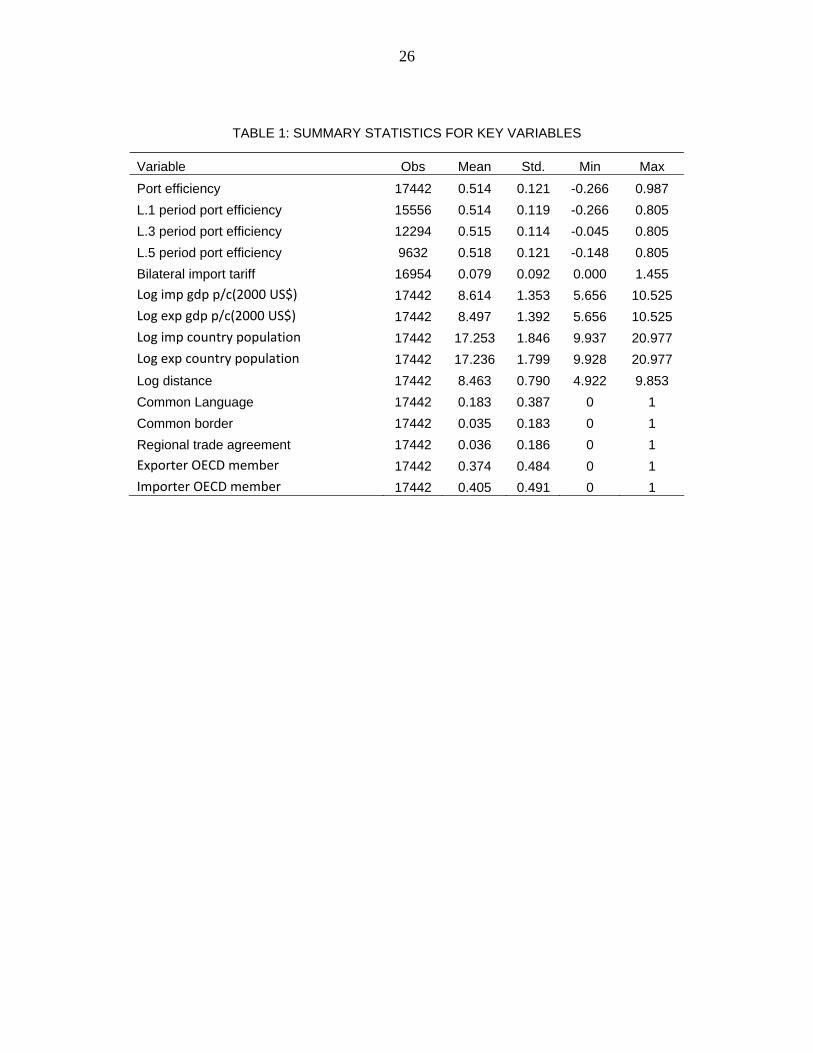
benchmark regression covers 41 countries, 819 country pairs, scans from 1991 to 2003. Table 1

gives the summary statistics on all major variables.

18

Hummels and Klenow (2005), who estimate cross-exporter extensive margins of

exports using a sample of single-year observations, show that large countries export more, not

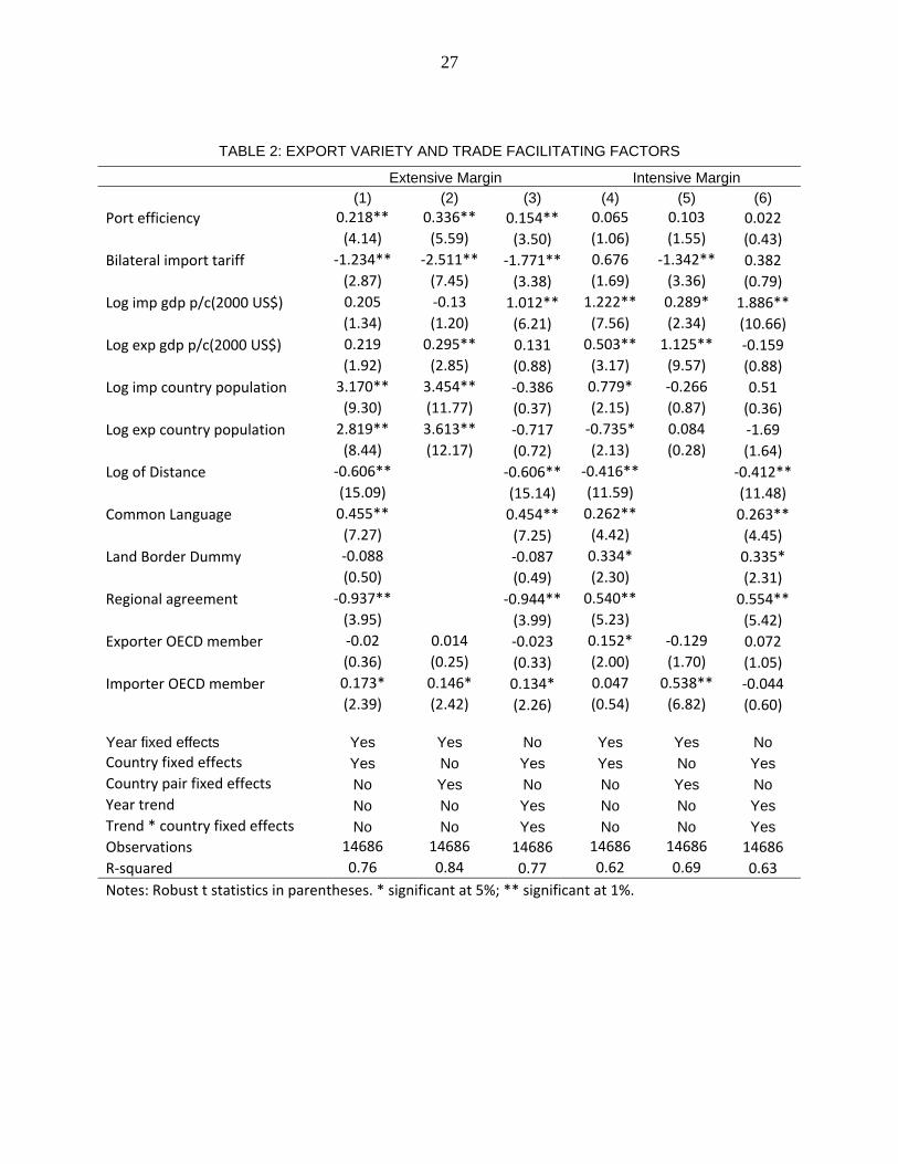
only in greater volume but also in a wider range. This is also confirmed by our benchmark

regression reported in Table 2. Furthermore, larger / richer countries also tend to import more,

both in volume and in variety range. Columns (1) and (4) give the basic specification showing

the positive and significant effect of port efficiency on trade in extensive margin, and positive

but insignificant effect on trade in intensive margin. To control for the possible under-estimation

of standard errors, we cluster the standard errors by importer-exporter pairs in the benchmark

specification and all following regressions.

The estimated coefficients are in line with our expectations. First, larger countries (in

GDP per capita and in population) tend to export more varieties and import more varieties. The

only exception is for exporting country’s population, which is negative. Second, having more

efficient ocean ports will substantially facilitate trade, this is more pronounced for trade in

variety, as in column (1). For intensive margin of export, the coefficient is positive but not

significant, as in column (4). Furthermore, bilateral import tariff significantly reduces exports in

extensive margin. In summary, improving ports efficiency by 10 percent increases export variety

by 2.18 percent, and increases intensive margin of export by 0.65 percent. A drop of 10 percent

in average bilateral import tariff leads to an increase in export variety by 12.3 percent, while the

intensive margin of export decreases by 6.8 percent. Notice that the intensive margin of exports

from i to j is measured as the bilateral exports relative to the world’s average exports to the same

importing country in the product categories exported from i to j, thus a positive coefficient of

port efficiency on the intensive margin does not necessarily mean trade costs such as tariffs

promote trade volume in absolute values.

19

Not surprisingly, being more distant form each other significantly reduced trade, in both

extensive and intensive margins. While speaking the same language appears to promote trade in

both margins. Moreover, if two countries are geographically contiguous, or have regional trade

agreement with each other, they trade more in intensive margin, rather than in extensive margin.

Interestingly, it seems that importing country’s OECD membership matters more than exporting

country’s, especially for the extensive margin of exports. This indicates that, controlling for other

factors, OECD countries (i.e., developed countries) demand much more varieties than non-

OECD countries (i.e., developing countries).

In columns (2) and (5), we add country pair fixed effects, aiming to control for all time-

invariant factors (both observed and unobserved) pertaining to the country pair. This treatment

makes the identification of bilateral port efficiency coefficient only depend on time series

variation and takes out all time-invariant features (both observed and unobserved) such as border

dummy, distance, etc. Benchmark results are confirmed. Efficient ocean ports help facilitating

export in variety while has not much to do with promoting relative export volume.

One concern with using country fixed effects or country pair fixed effects is that it does

not adequately control for time varying “multilateral resistance effects”, as pointed out in

Anderson and van Wincoop (2003) and Baldwin and Taglioni (2006). To deal with this, in

columns (3) and (6) we use a time trend, country fixed effects, as well as the interaction between

time trend and country dummies7. The results confirm the previous estimations that port

efficiency substantially promotes trade in extensive, though to a lower magnitude. 10 percent

improvement in port efficiency leads to 1.5 percent increase in the extensive margin of exports.

7 Ideally we should use country-year fixed effects. However, given the limited variation of our sample, using country-year fixed effects generates serious multicollinearity problem.

20

Furthermore, lowering bilateral import tariff also significantly promotes extensive margin of

exports.

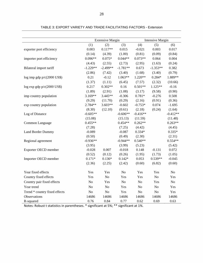
In Table 3, we further separate the importer port efficiency and the exporter port

efficiency.8 The findings are mostly consistent with those of Table 2. Furthermore, importer port

efficiency plays a substantial role in increasing the extensive margin of export from the source

country. The exporter port efficiency also matters but is not precisely estimated except for the

specification with country pair fixed effects. In most cases, both importer and exporter port

efficiency do not matter for the intensive margin of export.

Through Table 4 to Table 8, we investigate alternative specifications to our benchmark

model. We first investigate port efficiency and trade among OECD member countries in Table 4.

Then in Table 5, we investigate a subsample where only the importing country affiliates to

OECD while the exporting country does not. Table 6 examines the case where only the exporting

country affiliates to OECD while the importing country does not. Finally in Table 7, we consider

the case where none of the trading partners belongs to OECD. We run three regressions for each

subsample. Column (1) redoes the regression as specified in (16) but only use a subsample of

data. Columns (2) and (3) run the same regression, lagging port efficiency by 3 years and 5

years, respectively9. This is to at least partially control for the potential endogeneity of port

efficiency --- countries that have large trade transactions with each other are more likely to invest

to improve port efficiency. Then columns (4) to (6) repeat the same regression from columns (1)

to (3), with the intensive margin of exports as dependent variable.

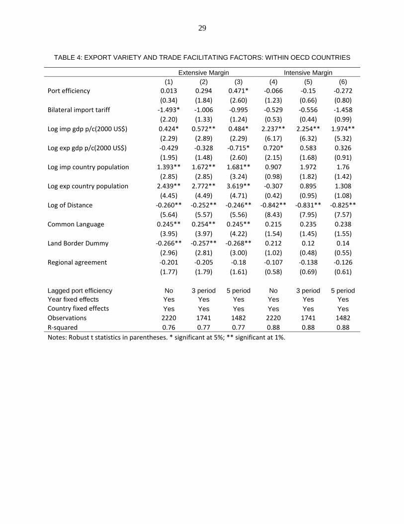
It is expected that more trade in varieties will be observed among industrial countries,

rather than between North-South country pairs or among South countries. This is because intra-

8 We thank an anonymous referee for suggesting this estimation. 9 Lag by 1 year gives similar results as using current year port efficiency.

21

industry trade, which is mainly in differentiated products, is dominant between the industrial

nations, who have similar income levels and consumer preference. In columns (1) and (4) Table

4, we redo the regression as specified in (16) but only look at trade among OECD countries.

Countries who are OECD member are on average larger and richer than non-OECD countries,

and trade between two OECD members is expected to be more pronounced in differentiated

products and more on the extensive margin. As expected, the importing country’s GDP per

capita has more pronounced positive effect than that of the full sample. On the other hand, the

coefficient of port inefficiency becomes insignificant, probably reflecting the fact that high level

of ports efficiency has already been obtained within OECD. When we are using lagged port

efficiency, it regains significance as in column (3)

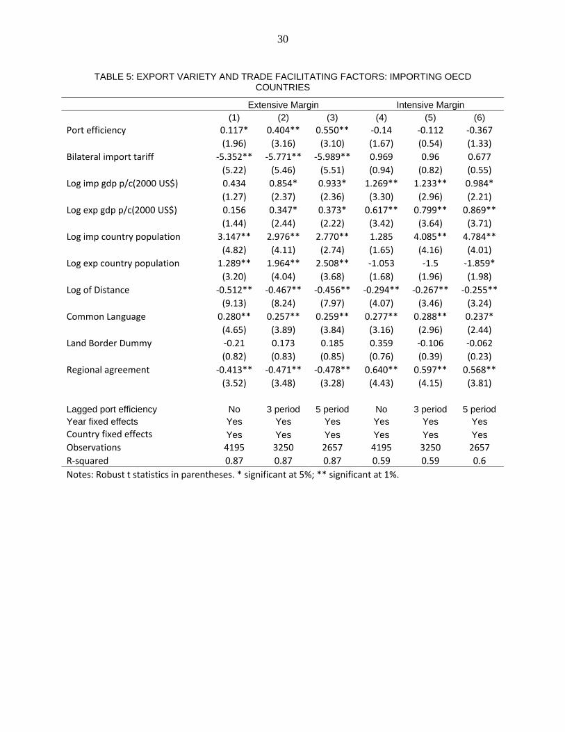
Table 5 examines the case in which only the importing country is OECD member. In

this case, port efficiency significantly promotes exports in extensive margin, while bilateral

import tariff significantly discourages exports in extensive margin. And both variables have no

significant effects on trade in intensive margin. In this case, GDP per capita and population of

both importing country (OECD member) and exporting country (non-OECD member) become

important in determining export variety.

Table 6 is the other side of the coin for Table 5: in this case, exporting country is

OECD member while importing country is not. Estimates of port efficiency show the same

pattern as in the benchmark regression and Table 5, when we use lagged measures of port

efficiency. However, the coefficients on tariff are controversially positive for both extensive and

intensive margins. This reflects that for less developed importing countries, higher tariff

probably makes it even harder to import from other less developed countries and therefore

relative increases imports from OECD countries in both margins.

22

Table 7 examines trade between non-OECD country pairs. This time, port efficiency is

positive and marginally significant (at 10% level) in promoting export variety in column (1),

while bilateral import tariff has negative and significant effect on export variety.

In regressions shown in Table 2 to Table 7, trade flows are not distinguished by its

transport mode. This potential raises doubt on the validity of using ocean ports efficiency

measure adopted from Blonigen and Wilson (2008). Due to lack of detailed data on trade with

different transport modes, we instead investigate a special case where no country pairs share any

common border, shown in Table 8. Most of the regression estimates are quite similar in

magnitude and in economic meaning to the story that Table 2 delivers, and are not discussed in

detail.

It is interesting to note that the coefficient estimates for RTAs show diverging patterns

for estimations with different groups of countries. Namely, for our benchmark regressions

(Tables 2 and 3) with all countries, or regressions with OECD importing countries, or regressions

with countries that do not share common borders, RTAs seem to discourage the export at the

extensive margin while increase the export at the intensive margin (the effect is similar but

weaker in significance for countries pairs with OECD exporting countries). But the effects of

RTAs seem to be small, both econometrically and economically, for OECD country pairs. Yet

the RTAs matter positively and substantially for both the extensive margin and intensive margin

for non-OECD country pairs. This seems to suggest for non-OECD countries, to facilitate trade,

it is very important to have good institutional arrangement such as regional trade agreements.

Since those countries are starting to be integrated into the world trade system, RTAs help

increase their exports at both margins. In contrast, trade within OECD countries does not depend

23

on RTAs, since they are already very integrated with each other. Indeed the largest RTA within

OECD countries is the European Union, which vary little during our sample period.

6. Conclusions

International trade provides an important engine for countries’ development and

productivity growth. The importance of lowering trade costs and facilitating trade are now

increasingly recognized by governments as well as academia. Yet questions like what factors

contribute the most to facilitating trade, or what policies should be in countries’ priority list to

lower trade costs and facilitate trade haven’t been answered satisfactorily. This project aims to

provide some empirical evidence on the impacts of different sources of trade costs on trade, in

particular, on the extensive margin of trade.

We construct an empirical gravity regression model to address the impact of ocean ports

efficiency, trade restrictiveness, international institutions such as OECD and RTA. An

improvement in port operating efficiency tends to increase export variety, especially when at

least one of the trade partners is not OECD country. A reduction in bilateral import tariff also

promotes trade in extensive margin in most cases. Being OECD members seems promote range

of export variety a great deal. While our further specification using smaller sample or changing

dependent variable gives weaker results, we believe that port inefficiency and tariff, which is a

simple average of product line tariffs, contribute significantly to trade costs. Removing those

trade costs, which also include but are not limit to standardization of various goods classification

system, harmonization of varying standards across nations, larger investment and better

technology to reduce information asymmetry, etc., would be a major project of cross-nation

cooperation. Among others, international institutions such as RTA, OECD, etc., should play

important roles promoting these policies and facilitating trade.

24

Acknowledgements: The authors thank an anonymous referee for helpful comments, and Bruce

Blonigen for providing the data on port efficiency.

References

Anderson, J. and E. van Wincoop (2003) “Trade Costs”, American Economic Review, 42:3, 691-

741.

Amurgo-Pacheco, A. and M. Pierola (2008) “Patterns of Exporting Diversification in Developing

Countries: Intensive and Extensive Margins.”, World Bank Policy Research Working Paper

No.4473.

Baldwin, R. and V. Di Nino (2006) “Euros and Zeros: the Common Currency Effect on Trade in

New Goods”, NBER Working Paper No. 12673.

Baldwin, R. and D. Taglioni (2006) “Gravity for Dummies and Dummies for Gravity

Equations”, NBER Working Paper No. 12516.

Bergin, P. and C. Lin (2009) "Exchange Rate Regimes and the Extensive Margin of Trade,"

NBER Chapters, in: NBER International Seminar on Macroeconomics 2008, pages 201-227

National Bureau of Economic Research, Inc.

Bernard, A. B., J. B. Jensen, S. Redding and P. K. Schott (2007) “Firms in International Trade,”

Journal of Economic Perspectives, summer.

Blonigen, B. and W. Wilson (2008) “Port Efficiency and Trade Flows”, Review of International

Economics. Vol.16: 21-36.

Broda, C. and D. E. Weinstein (2006) “Globalization and the Gain from Trade,” Quarterly

Journal of Economics, 121: 541-585.

Chen, X., T. Otsuki, and J. Wilson (2008) "Standards and export decisions: Firm-level evidence

from developing countries," Journal of International Trade & Economic Development, vol.

17(4): 501-523.

Clark, X., D. Dollar and A. Micco (2004) “Port Efficiency, Maritime Transport Costs and

Bilateral Trade”, NBER Working Paper 10353.

Dennis, A. and B. Shepherd (2007) “Trade Costs, Barriers to Entry, and Export Diversification

in Developing Countries”, World Bank Policy Research Working Paper No. 4368.

25

Eaton, J., S. Kortum, and F. Kramarz (2004) “Dissecting Trade: Firms, Industries, and Export

Destinations”, American Economic Review 94(2):150-154.

Feenstra, R. C. (1994) “New Product Varieties and the Measurement of International Prices”,

American Economic Review, 84(1):157-177.

Feenstra, R.C. and H.-L. Kee (2008) “Export Variety and Country Productivity: Estimating the

Monopolistic Competition Model with Endogenous Productivity”, Journal of International

Economics 74(2):500-514.

Hummels, D. L. and P. J. Klenow (2005) “The Variety and Quality of a Nation's Trade,”

American Economic Review, 95(3): 704-723.

Kee, H.-L., A. Nicita, and M. Olarreaga (2009) “Estimating Trade Restrictiveness Indices”,

Economic Journal, 119(534):172-99.

Kehoe, T. and K. Ruhl (2004) “ How Important is the New Goods Margin in International

Trade?”, Mimeo, University of Minnesota.

Limao, N. and A. Venables (2000) “Infrastructure, Geographical Disadvantage and Transport

Costs”, The World Bank Economic Review, 15(3): 451-479.

Melitz, M. J. (2003) “The Impact of Trade on Intra-Industry Reallocations and Aggregate

Industry Productivity”, Econometrica, 71(6):1695-1725

Rose, A. (2004) “Do We Really Know That the WTO Increases Trade?”, American Economic

Review, 94(1): 98-114.

Sato, K. (1976) “The Ideal Log-Change Index Number”, Review of Economics and Statistics 58

(May): 223–228.

Shepherd, B. and J. Wilson (2006) “Road Infrastructure in Europe and Central Asia: Does

Network Quality Affect Trade?”, World Bank Policy Research Working Paper 4104.

Soloaga, I., J. Wilson, and A. Mejia (2006) “Moving Forward Faster: Trade Facilitation Reform

and Mexican Competitiveness”, World Bank Policy Research Working Paper 3953.

Subramanian, A. and S.-J. Wei (2007) “The WTO Promotes Trade, Strongly but Unevenly”,

Journal of International Economics, 72: 151-175.

Vartia, Y. O. (1976) “Ideal Log-Change Index Numbers”. Scandinavian Journal of Statistics 3

(3): 121–126.

Wilson, J., C. Mann and T. Otsuki (2005) “Assessing the Benefits of Trade Facilitation: A

Global Perspective”, The World Economy, 28(6): 841-871

26

TABLE 1: SUMMARY STATISTICS FOR KEY VARIABLES

Variable Obs Mean Std. Min Max

Port efficiency 17442 0.514 0.121 -0.266 0.987

L.1 period port efficiency 15556 0.514 0.119 -0.266 0.805



Bilateral import tariff 16954 0.079 0.092 0.000 1.455

Log imp gdp p/c(2000 US$) 17442 8.614 1.353 5.656 10.525

Log exp gdp p/c(2000 US$) 17442 8.497 1.392 5.656 10.525

Log imp country population 17442 17.253 1.846 9.937 20.977

Log exp country population 17442 17.236 1.799 9.928 20.977

Log distance 17442 8.463 0.790 4.922 9.853

Common Language 17442 0.183 0.387 0 1

Common border 17442 0.035 0.183 0 1

Regional trade agreement 17442 0.036 0.186 0 1

Exporter OECD member 17442 0.374 0.484 0 1

Importer OECD member 17442 0.405 0.491 0 1

27

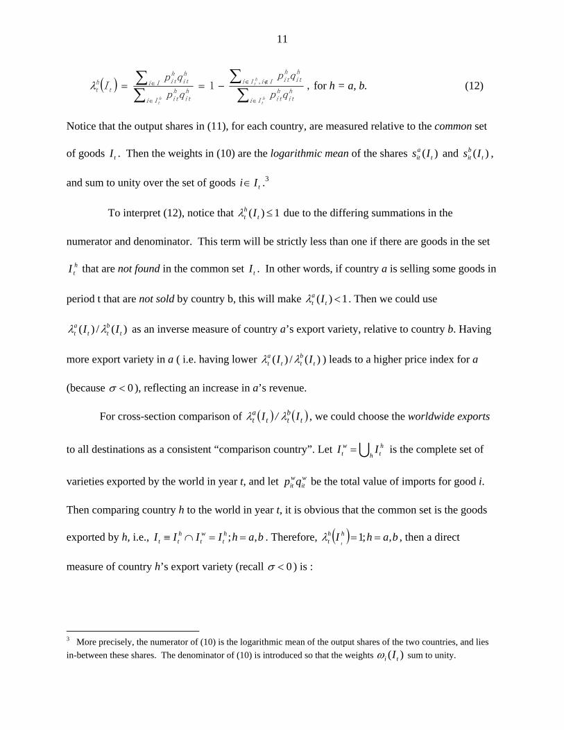
TABLE 2: EXPORT VARIETY AND TRADE FACILITATING FACTORS

Extensive Margin Intensive Margin (1) (2) (3) (4) (5) (6) Port efficiency 0.218** 0.336** 0.154** 0.065 0.103 0.022

(4.14) (5.59) (3.50) (1.06) (1.55) (0.43)

Bilateral import tariff ‐1.234** ‐2.511** ‐1.771** 0.676 ‐1.342** 0.382

(2.87) (7.45) (3.38) (1.69) (3.36) (0.79)

Log imp gdp p/c(2000 US$) 0.205 ‐0.13 1.012** 1.222** 0.289* 1.886**

(1.34) (1.20) (6.21) (7.56) (2.34) (10.66)

Log exp gdp p/c(2000 US$) 0.219 0.295** 0.131 0.503** 1.125** ‐0.159

(1.92) (2.85) (0.88) (3.17) (9.57) (0.88)

Log imp country population 3.170** 3.454** ‐0.386 0.779* ‐0.266 0.51

(9.30) (11.77) (0.37) (2.15) (0.87) (0.36)

Log exp country population 2.819** 3.613** ‐0.717 ‐0.735* 0.084 ‐1.69

(8.44) (12.17) (0.72) (2.13) (0.28) (1.64)

Log of Distance ‐0.606** ‐0.606** ‐0.416** ‐0.412**

(15.09) (15.14) (11.59) (11.48)

Common Language 0.455** 0.454** 0.262** 0.263**

(7.27) (7.25) (4.42) (4.45)

Land Border Dummy ‐0.088 ‐0.087 0.334* 0.335*

(0.50) (0.49) (2.30) (2.31)

Regional agreement ‐0.937** ‐0.944** 0.540** 0.554**

(3.95) (3.99) (5.23) (5.42)

Exporter OECD member ‐0.02 0.014 ‐0.023 0.152* ‐0.129 0.072

(0.36) (0.25) (0.33) (2.00) (1.70) (1.05)

Importer OECD member 0.173* 0.146* 0.134* 0.047 0.538** ‐0.044

(2.39) (2.42) (2.26) (0.54) (6.82) (0.60) Year fixed effects Yes Yes No Yes Yes No Country fixed effects Yes No Yes Yes No Yes Country pair fixed effects No Yes No No Yes No Year trend No No Yes No No Yes Trend * country fixed effects No No Yes No No Yes Observations 14686 14686 14686 14686 14686 14686

R‐squared 0.76 0.84 0.77 0.62 0.69 0.63

Notes: Robust t statistics in parentheses. * significant at 5%; ** significant at 1%.

28

TABLE 3: EXPORT VARIETY AND TRADE FACILITATING FACTORS - Extension

Extensive Margin Intensive Margin (1) (2) (3) (4) (5) (6) exporter port efficiency 0.003 0.117** 0.015 -0.021 0.003 0.017 (0.14) (4.39) (1.00) (0.81) (0.09) (0.84) importer port efficiency 0.096** 0.075* 0.044** 0.073** 0.064 0.004 (4.43) (2.55) (2.73) (2.95) (1.63) (0.24) Bilateral import tariff -1.229** -2.499** -1.781** 0.673 -1.353** 0.382 (2.86) (7.42) (3.40) (1.68) (3.40) (0.79) log imp gdp p/c(2000 US$) 0.21 -0.12 1.063** 1.220** 0.284* 1.889** (1.37) (1.11) (6.45) (7.57) (2.32) (10.66) log exp gdp p/c(2000 US$) 0.217 0.302** 0.16 0.501** 1.125** -0.16 (1.89) (2.91) (1.08) (3.17) (9.58) (0.90) imp country population 3.169** 3.445** -0.306 0.781* -0.276 0.508 (9.29) (11.70) (0.29) (2.16) (0.91) (0.36) exp country population 2.784** 3.603** -0.602 -0.753* 0.074 -1.695 (8.30) (12.10) (0.61) (2.18) (0.24) (1.64) Log of Distance -0.605** -0.606** -0.416** -0.412** (15.08) (15.13) (11.59) (11.48) Common Language 0.455** 0.454** 0.262** 0.263** (7.28) (7.25) (4.42) (4.45) Land Border Dummy -0.089 -0.087 0.334* 0.335* (0.50) (0.49) (2.30) (2.31) Regional agreement -0.936** -0.944** 0.540** 0.554** (3.95) (3.99) (5.23) (5.42) Exporter OECD member -0.028 0.007 -0.018 0.148 -0.131 0.072 (0.52) (0.12) (0.26) (1.95) (1.73) (1.05) Importer OECD member 0.171* 0.136* 0.142* 0.053 0.539** -0.045 (2.36) (2.25) (2.42) (0.60) (6.82) (0.60) Year fixed effects Yes Yes No Yes Yes No Country fixed effects Yes No Yes Yes No Yes

Country pair fixed effects No Yes No No Yes No

Year trend No No Yes No No Yes

Trend * country fixed effects No No Yes No No Yes Observations 14686 14686 14686 14686 14686 14686 R-squared 0.76 0.84 0.77 0.62 0.69 0.63 Notes: Robust t statistics in parentheses. * significant at 5%; ** significant at 1%.

29

TABLE 4: EXPORT VARIETY AND TRADE FACILITATING FACTORS: WITHIN OECD COUNTRIES

Extensive Margin Intensive Margin (1) (2) (3) (4) (5) (6) Port efficiency 0.013 0.294 0.471* ‐0.066 ‐0.15 ‐0.272

(0.34) (1.84) (2.60) (1.23) (0.66) (0.80)

Bilateral import tariff ‐1.493* ‐1.006 ‐0.995 ‐0.529 ‐0.556 ‐1.458

(2.20) (1.33) (1.24) (0.53) (0.44) (0.99)

Log imp gdp p/c(2000 US$) 0.424* 0.572** 0.484* 2.237** 2.254** 1.974**

(2.29) (2.89) (2.29) (6.17) (6.32) (5.32)

Log exp gdp p/c(2000 US$) ‐0.429 ‐0.328 ‐0.715* 0.720* 0.583 0.326

(1.95) (1.48) (2.60) (2.15) (1.68) (0.91)

Log imp country population 1.393** 1.672** 1.681** 0.907 1.972 1.76

(2.85) (2.85) (3.24) (0.98) (1.82) (1.42)

Log exp country population 2.439** 2.772** 3.619** ‐0.307 0.895 1.308

(4.45) (4.49) (4.71) (0.42) (0.95) (1.08)

Log of Distance ‐0.260** ‐0.252** ‐0.246** ‐0.842** ‐0.831** ‐0.825**

(5.64) (5.57) (5.56) (8.43) (7.95) (7.57)

Common Language 0.245** 0.254** 0.245** 0.215 0.235 0.238

(3.95) (3.97) (4.22) (1.54) (1.45) (1.55)

Land Border Dummy ‐0.266** ‐0.257** ‐0.268** 0.212 0.12 0.14

(2.96) (2.81) (3.00) (1.02) (0.48) (0.55)

Regional agreement ‐0.201 ‐0.205 ‐0.18 ‐0.107 ‐0.138 ‐0.126

(1.77) (1.79) (1.61) (0.58) (0.69) (0.61)

Lagged port efficiency No 3 period 5 period No 3 period 5 period Year fixed effects Yes Yes Yes Yes Yes Yes Country fixed effects Yes Yes Yes Yes Yes Yes Observations 2220 1741 1482 2220 1741 1482

R‐squared 0.76 0.77 0.77 0.88 0.88 0.88


30

TABLE 5: EXPORT VARIETY AND TRADE FACILITATING FACTORS: IMPORTING OECD COUNTRIES

Extensive Margin Intensive Margin (1) (2) (3) (4) (5) (6) Port efficiency 0.117* 0.404** 0.550** ‐0.14 ‐0.112 ‐0.367

(1.96) (3.16) (3.10) (1.67) (0.54) (1.33)

Bilateral import tariff ‐5.352** ‐5.771** ‐5.989** 0.969 0.96 0.677

(5.22) (5.46) (5.51) (0.94) (0.82) (0.55)

Log imp gdp p/c(2000 US$) 0.434 0.854* 0.933* 1.269** 1.233** 0.984*

(1.27) (2.37) (2.36) (3.30) (2.96) (2.21)

Log exp gdp p/c(2000 US$) 0.156 0.347* 0.373* 0.617** 0.799** 0.869**

(1.44) (2.44) (2.22) (3.42) (3.64) (3.71)

Log imp country population 3.147** 2.976** 2.770** 1.285 4.085** 4.784**

(4.82) (4.11) (2.74) (1.65) (4.16) (4.01)

Log exp country population 1.289** 1.964** 2.508** ‐1.053 ‐1.5 ‐1.859*

(3.20) (4.04) (3.68) (1.68) (1.96) (1.98)

Log of Distance ‐0.512** ‐0.467** ‐0.456** ‐0.294** ‐0.267** ‐0.255**

(9.13) (8.24) (7.97) (4.07) (3.46) (3.24)

Common Language 0.280** 0.257** 0.259** 0.277** 0.288** 0.237*

(4.65) (3.89) (3.84) (3.16) (2.96) (2.44)

Land Border Dummy ‐0.21 0.173 0.185 0.359 ‐0.106 ‐0.062

(0.82) (0.83) (0.85) (0.76) (0.39) (0.23)

Regional agreement ‐0.413** ‐0.471** ‐0.478** 0.640** 0.597** 0.568**

(3.52) (3.48) (3.28) (4.43) (4.15) (3.81)


R‐squared 0.87 0.87 0.87 0.59 0.59 0.6


31

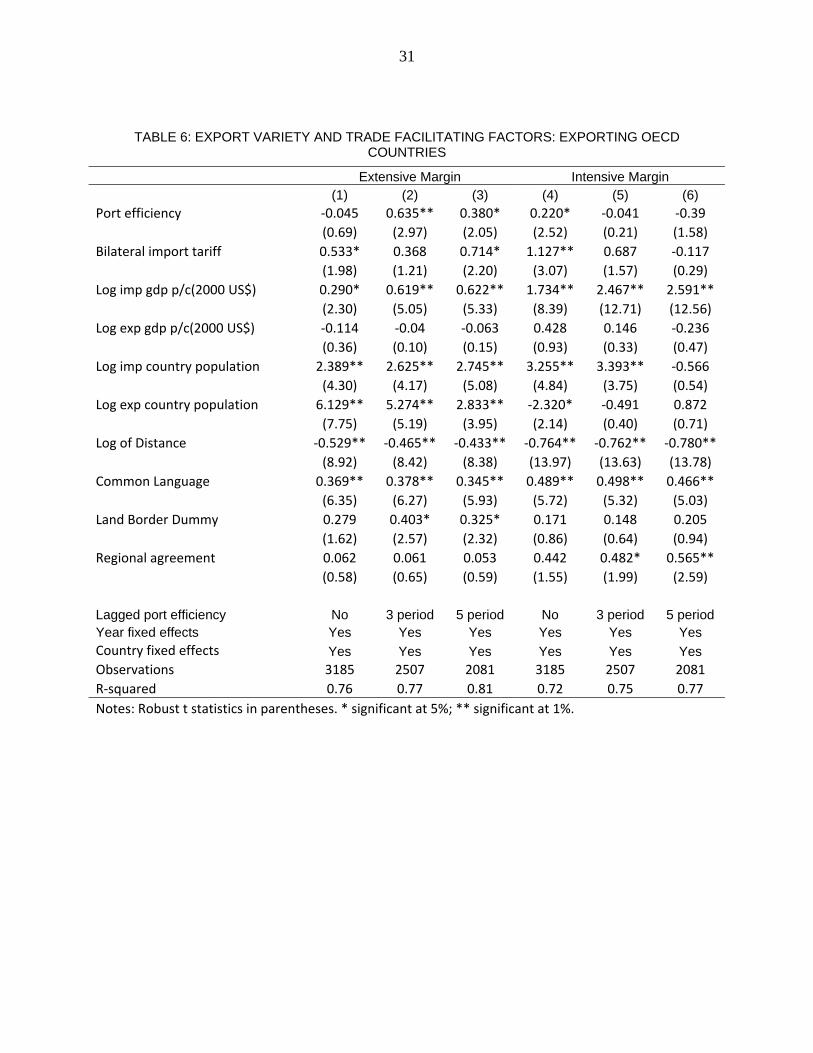
TABLE 6: EXPORT VARIETY AND TRADE FACILITATING FACTORS: EXPORTING OECD COUNTRIES

Extensive Margin Intensive Margin (1) (2) (3) (4) (5) (6) Port efficiency ‐0.045 0.635** 0.380* 0.220* ‐0.041 ‐0.39

(0.69) (2.97) (2.05) (2.52) (0.21) (1.58)

Bilateral import tariff 0.533* 0.368 0.714* 1.127** 0.687 ‐0.117

(1.98) (1.21) (2.20) (3.07) (1.57) (0.29)

Log imp gdp p/c(2000 US$) 0.290* 0.619** 0.622** 1.734** 2.467** 2.591**

(2.30) (5.05) (5.33) (8.39) (12.71) (12.56)

Log exp gdp p/c(2000 US$) ‐0.114 ‐0.04 ‐0.063 0.428 0.146 ‐0.236

(0.36) (0.10) (0.15) (0.93) (0.33) (0.47)

Log imp country population 2.389** 2.625** 2.745** 3.255** 3.393** ‐0.566

(4.30) (4.17) (5.08) (4.84) (3.75) (0.54)

Log exp country population 6.129** 5.274** 2.833** ‐2.320* ‐0.491 0.872

(7.75) (5.19) (3.95) (2.14) (0.40) (0.71)

Log of Distance ‐0.529** ‐0.465** ‐0.433** ‐0.764** ‐0.762** ‐0.780**

(8.92) (8.42) (8.38) (13.97) (13.63) (13.78)

Common Language 0.369** 0.378** 0.345** 0.489** 0.498** 0.466**

(6.35) (6.27) (5.93) (5.72) (5.32) (5.03)

Land Border Dummy 0.279 0.403* 0.325* 0.171 0.148 0.205

(1.62) (2.57) (2.32) (0.86) (0.64) (0.94)

Regional agreement 0.062 0.061 0.053 0.442 0.482* 0.565**

(0.58) (0.65) (0.59) (1.55) (1.99) (2.59)


R‐squared 0.76 0.77 0.81 0.72 0.75 0.77


32

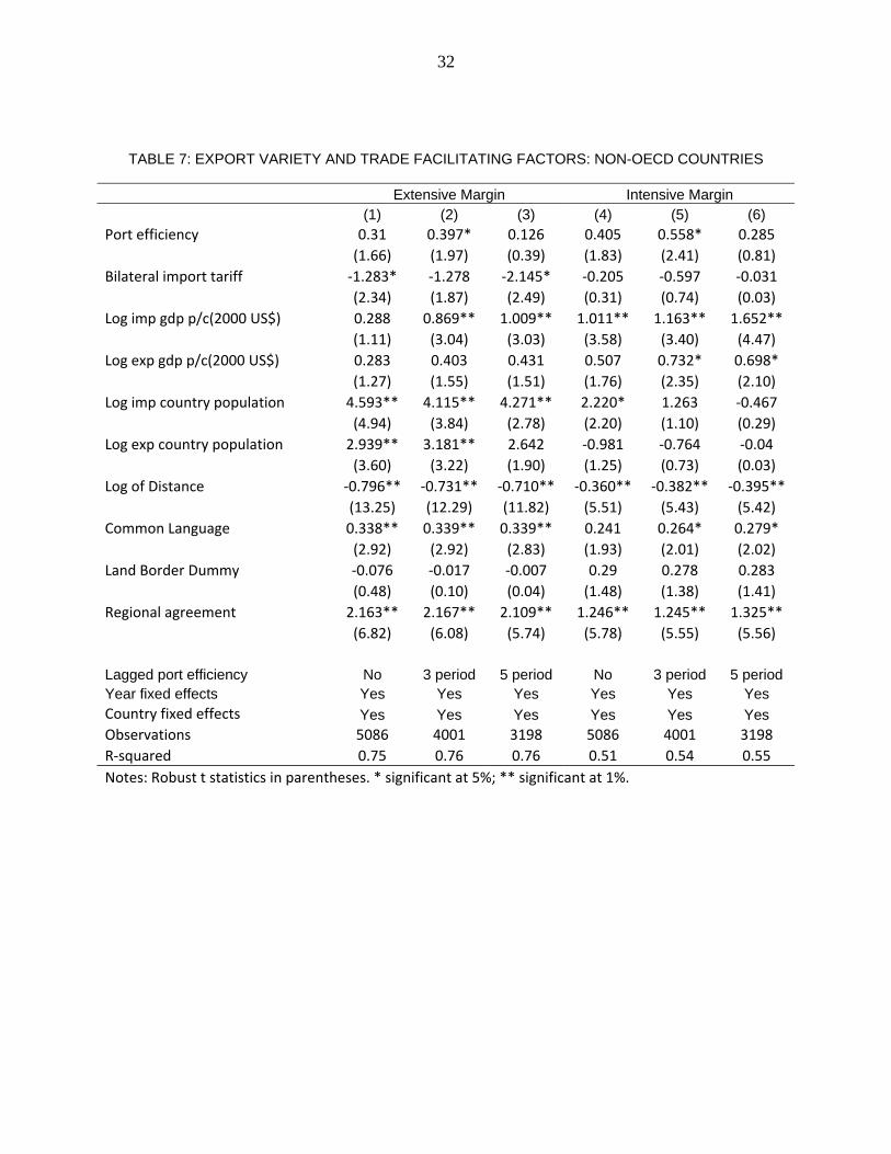
TABLE 7: EXPORT VARIETY AND TRADE FACILITATING FACTORS: NON-OECD COUNTRIES

Extensive Margin Intensive Margin (1) (2) (3) (4) (5) (6) Port efficiency 0.31 0.397* 0.126 0.405 0.558* 0.285

(1.66) (1.97) (0.39) (1.83) (2.41) (0.81)

Bilateral import tariff ‐1.283* ‐1.278 ‐2.145* ‐0.205 ‐0.597 ‐0.031

(2.34) (1.87) (2.49) (0.31) (0.74) (0.03)

Log imp gdp p/c(2000 US$) 0.288 0.869** 1.009** 1.011** 1.163** 1.652**

(1.11) (3.04) (3.03) (3.58) (3.40) (4.47)

Log exp gdp p/c(2000 US$) 0.283 0.403 0.431 0.507 0.732* 0.698*

(1.27) (1.55) (1.51) (1.76) (2.35) (2.10)

Log imp country population 4.593** 4.115** 4.271** 2.220* 1.263 ‐0.467

(4.94) (3.84) (2.78) (2.20) (1.10) (0.29)

Log exp country population 2.939** 3.181** 2.642 ‐0.981 ‐0.764 ‐0.04

(3.60) (3.22) (1.90) (1.25) (0.73) (0.03)

Log of Distance ‐0.796** ‐0.731** ‐0.710** ‐0.360** ‐0.382** ‐0.395**

(13.25) (12.29) (11.82) (5.51) (5.43) (5.42)

Common Language 0.338** 0.339** 0.339** 0.241 0.264* 0.279*

(2.92) (2.92) (2.83) (1.93) (2.01) (2.02)

Land Border Dummy ‐0.076 ‐0.017 ‐0.007 0.29 0.278 0.283

(0.48) (0.10) (0.04) (1.48) (1.38) (1.41)

Regional agreement 2.163** 2.167** 2.109** 1.246** 1.245** 1.325**

(6.82) (6.08) (5.74) (5.78) (5.55) (5.56)


R‐squared 0.75 0.76 0.76 0.51 0.54 0.55


33

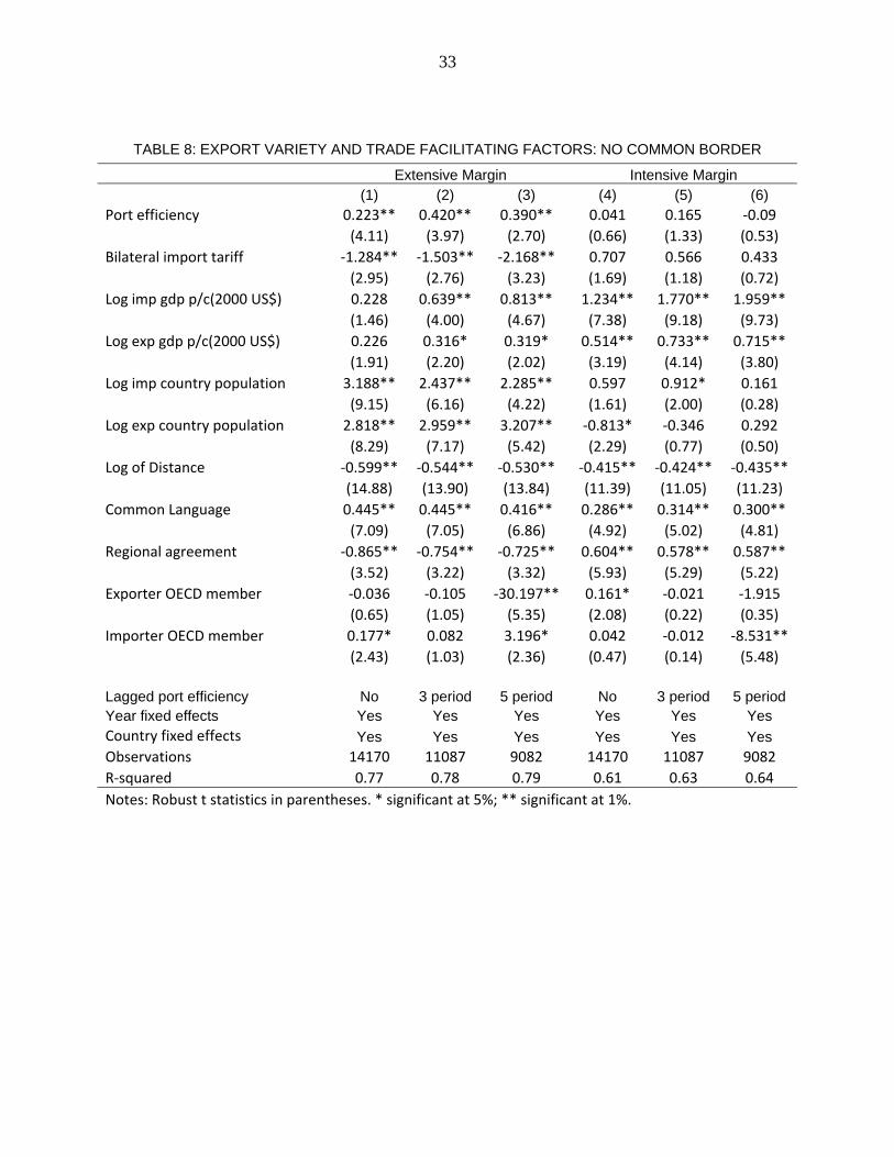
TABLE 8: EXPORT VARIETY AND TRADE FACILITATING FACTORS: NO COMMON BORDER

Extensive Margin Intensive Margin (1) (2) (3) (4) (5) (6) Port efficiency 0.223** 0.420** 0.390** 0.041 0.165 ‐0.09

(4.11) (3.97) (2.70) (0.66) (1.33) (0.53)

Bilateral import tariff ‐1.284** ‐1.503** ‐2.168** 0.707 0.566 0.433

(2.95) (2.76) (3.23) (1.69) (1.18) (0.72)

Log imp gdp p/c(2000 US$) 0.228 0.639** 0.813** 1.234** 1.770** 1.959**

(1.46) (4.00) (4.67) (7.38) (9.18) (9.73)

Log exp gdp p/c(2000 US$) 0.226 0.316* 0.319* 0.514** 0.733** 0.715**

(1.91) (2.20) (2.02) (3.19) (4.14) (3.80)

Log imp country population 3.188** 2.437** 2.285** 0.597 0.912* 0.161

(9.15) (6.16) (4.22) (1.61) (2.00) (0.28)

Log exp country population 2.818** 2.959** 3.207** ‐0.813* ‐0.346 0.292

(8.29) (7.17) (5.42) (2.29) (0.77) (0.50)

Log of Distance ‐0.599** ‐0.544** ‐0.530** ‐0.415** ‐0.424** ‐0.435**

(14.88) (13.90) (13.84) (11.39) (11.05) (11.23)

Common Language 0.445** 0.445** 0.416** 0.286** 0.314** 0.300**

(7.09) (7.05) (6.86) (4.92) (5.02) (4.81)

Regional agreement ‐0.865** ‐0.754** ‐0.725** 0.604** 0.578** 0.587**

(3.52) (3.22) (3.32) (5.93) (5.29) (5.22)

Exporter OECD member ‐0.036 ‐0.105 ‐30.197** 0.161* ‐0.021 ‐1.915

(0.65) (1.05) (5.35) (2.08) (0.22) (0.35)

Importer OECD member 0.177* 0.082 3.196* 0.042 ‐0.012 ‐8.531**

(2.43) (1.03) (2.36) (0.47) (0.14) (5.48)


R‐squared 0.77 0.78 0.79 0.61 0.63 0.64


34

C

B

q2

q1A

D

Figure 2: Gains from Output Variety

Figure 1: Gains from Consumer Variety

B

C

q2

D

A q1

Documents

Trade Facilitation and the Extensive Margin-Finalcid.econ.ucdavis.edu/Papers/Trade_Facilitation_and_the_Extensive... · Trade Facilitation and the Extensive Margin of Exports Robert