Trade Finance and the Durability of theDollar∗

Ryan ChahrourBoston College

Rosen ValchevBoston College

October 1, 2021

Abstract

We propose a model in which the emergence of a single dominant currency isdriven by the need to finance international trade. The model generates multiple stablesteady states, each characterized by a different dominant asset, consistent with thehistorical durability of real-world currency regimes. The persistence of regimes iscaused by a positive interaction between the returns to saving in an asset and the useof that asset for financing trade. A calibrated version of the model shows that thewelfare gains of dominance are substantial, but accrue primarily during the transitionto dominance. We perform several counterfactual experiments to assess potentialthreats to the dollar’s continued dominance.

JEL Codes: E44, F02, F33, F41, G15

Keywords: trade finance; dollar dominance; exorbitant privilege; liquidity pre-mium; global imbalances

∗This paper originally circulated as Boston College Working Paper 934. We are grateful to our discussants,Ozge Akinci, Saleem Bahaj, Matteo Maggiori, Federica Romei, Adrien Verdelhan and Martin Wolf, and toseminar participants at the AEA annual meetings, Banque de France, Barcelona Summer Forum, BostonMacro Juniors Workshop, Boston University, CEBRA 2021, CEF, Chicago Booth IFM, EACBN-Mannheim,the Federal Reserve Banks of Boston, Dallas, Chicago, Richmond, and Philadelphia, Fordham Conference onMacroeconomics and International Finance, Harvard University, Indiana University, the Konstanz Seminaron Monetary Theory and Monetary Policy, the Spring 2018 NBER IFM, Oxford-Zurich Macrofinance 2021,SED, SEM, SFS, UQAM, University of Notre Dame, and the University of Wisconsin-Madison. We thankSherty Huang for excellent research assistance. Contact: ryan.chahrour@bc.edu, valchev@bc.edu.

1 Introduction

Historically, the international financial system has been characterized by long-lasting

periods in which one “dominant” asset facilitates the majority of international trade and

financial flows. Since the 1950s, this role has been played by the US dollar and safe US

assets, while the British pound enjoyed dominance before that, and the Dutch Guilder was

the dominant asset throughout the 18th century. This pattern suggests that the international

financial system favors the emergence of extended periods of currency dominance. The

potential for such dominance has been of great interest to prior literature, but the question

of why currency regimes often prove so durable has received comparatively little attention.

This paper provides a theory of stable dominant currency regimes. The theory relies on

two frictions in international trade, imperfect contract enforcement across borders, which

creates a need for collateral guarantees in trade, and a financial friction in obtaining the

needed collateral. Trading firms seek to borrow collateral via frictional trade finance markets,

generating a positive feedback between the use of an asset to guarantee trade and households’

incentives to save in that asset. Firms also benefit from operating with the same collateral

as their trade counterparties, which reinforces the household-firm complementarity. The

interaction of these forces gives rise to multiple steady states, each characterized by a different

dominant asset and surrounded by a region of unique, stable equilibrium dynamics.

Our model economy is composed of three regions: the United State, the Eurozone, and a

continuum of small, open, rest-of-world economies. In each country, there is a continuum of

trading firms seeking to engage in profitable transactions with traders from other countries.

Imperfect contract enforcement across borders requires the trading firms to collateralize their

transactions with safe assets that serve as performance guarantees. To obtain collateral, firms

seek an intra-period loan of either US or Eurozone bonds in domestic bond-specific search

and matching markets. On the other side of these credit markets are the local households,

who form optimal portfolios and offer intra-period loans from their asset holdings for a fee.

Other things equal, search frictions encourage firms to look for trade financing in the

credit market that is less tight, and thus apply for a loan of whichever asset forms a larger

share of domestic household portfolios. Conversely, households know that an asset that is

heavily used by traders is more likely to be loaned out in the trade finance markets and earn

the associated fee. Thus, the incentives of households and trading firms reinforce each other:

a large usage of an asset in trade finance encourages households to save in that asset, while

large portfolio holdings of the asset encourage firms to seek it for financing trade activities.

We begin our analysis by analytically characterizing the key forces driving dominance

1

and stability within a simplified model. First, we show that the feedback between households

and trading firms leads to steady-state multiplicity, including a dollar-dominant steady state

in which US safe assets are both the dominant saving vehicle of rest-of-world households

and the dominant means of trade finance. The other steady states are a mirror-image euro-

dominant steady state, and a “multi-polar” steady state in which portfolios and trade finance

use are split equally across the two assets.

While this firm-household interaction can generate dominant-currency steady states,

these outcomes may not be stable. Intuitively, when one asset dominates trade finance

activity, the market for loans of that asset is relatively congested. Hence, an off-equilibrium

shift in the portfolio composition of households can drive firms to shift their financing use

away from the dominant asset. To ensure stability, we introduce a currency mismatch cost

that is incurred by trading firm pairs who use different types of collateral. This cost can

be micro-founded as the expected cost of default by one of the transaction counterparties,

since mismatched collateral means the two promises may not be equivalent in all states of

the world.1

Collateral mismatch costs introduce a second strategic complementarity, now in the type

of financing sought by trading firms in different countries. On its own, this complementarity

would give rise to sunspot equilibria, since trade finance choices would depend only on what

firms expect their foreign counterparties to choose. Frictions in funding markets limit this

indeterminacy, however, because firms’ funding choices are also influenced by the relative

availability of different types of trade financing.

Crucially, the interaction between the two complementarity mechanisms – one between

households and firms, the other among firms – can make dominant-asset steady states locally

stable. Intuitively, wide holdings of an asset make it easier for firms to source it, giving it an

initial advantage in firms’ currency choices. This advantage is then reinforced by firms’ cross-

country coordination incentives, uniquely anchoring their currency choice on the widely-held

asset. Importantly, neither mechanism can achieve this on its own: Without both sources of

complementarity, equilibrium is either locally unstable or subject to sunspot indeterminacy.

Having illustrated the key mechanism, we embed it within a rich general equilibrium

model, and explore its quantitative implications in and out of steady state. We calibrate the

model to match target moments on the size of government debt, trade, currency denomina-

tion of trade finance, and import markups. The model exactly matches the target moments

and a number of additional, non-targeted moments are also closely aligned with the data.

Using the calibrated model, we first show that dominant-currency steady states in this

1Amiti et al. (2018) find evidence of such coordination incentives in firm-level trade data from Belgium.

2

richer, quantitative framework are indeed dynamically stable, and lie within large regions

of the state space that uniquely converge to their respective dominant-asset steady state.

Within those regions, the equilibrium paths of the economy are determinate (i.e. not subject

to sunspot shocks) and the currency regime is uniquely determined by initial conditions. Es-

sentially, the dynamic model tethers the mix of assets used for trade finance to an endogenous

state variable, the composition of rest-of-world bond portfolios, generating the co-existence

of distinct, stable dollar- and euro-dominant steady states. By contrast, we show that the

multi-polar steady state is unstable. Hence, the model implies that durable single-currency

regimes should predominate, just like in the historical record.

Computing the welfare implications of the model leads to several new insights that show-

case the importance of a dynamic general equilibrium analysis of currency dominance. The

steady-state gain of the dominant country, relative to the other large country, is small –

only 0.03% of permanent consumption – even though the equilibrium interest rate of the

dominant asset is roughly one percent lower than that of the other asset, consistent with

the data.2 In our general equilibrium model, this “exorbitant privilege” does not generate

a long-run welfare benefit because the low interest rate is a consequence of high external

demand for the dominant country’s assets, which also results in a negative net foreign asset

position for the country (as is also true in the data). In our calibration, the costs of servicing

this external imbalance roughly offset the benefits of paying lower interest.

Though dominance has a small effect on consumption in the long-run, factoring in the

transition to dominance dramatically changes welfare conclusions. For example, in the case

of a transition from the (unstable) symmetric steady state, the eventual dominant country

gains the equivalent of 0.75% of permanent consumption. This happens because, along the

transition path, increasing external demand for the assets of the dominant country helps it

to fund a temporary boom in consumption. This finding emphasizes the importance of using

a dynamic model to evaluate the positive consequences of currency dominance.

We conclude the paper with three counter-factual experiments. First, we analyze the for-

mation of the Eurozone, one of the most important recent developments in the international

financial system. Consistent with historical experience, the model shows that starting from a

point where the US is the only country furnishing safe assets on a global scale (and thus the

dollar-dominant steady state is unique), the introduction of an ex-ante equivalent Eurozone

2While our perfect foresight model does not differentiate between covered and uncovered interest parity(UIP), the spirit of our mechanism is most consistent with a violation of UIP. Trade collateral is required toguarantee future contract performance, thus the resulting convenience yield is earned by an asset’s abilityto insure a promised future dollar value, meaning synthetic dollar bonds and US dollar bonds are equivalentto one another, but different from euro bonds.

3

asset is not sufficient to precipitate a currency regime change: While the Eurozone forma-

tion does create a second stable dominant-asset steady state, the world is already dollarized

at the euro’s introduction, and nothing about the change pushes the world economy away

from its dollar-dominated starting point. More broadly, the model implies that we live in a

dollar-dominant world today due to the combination of path dependence and the stability of

dominance. Still, the dollar’s dominant position is not guaranteed, and future shocks could

push the economy into the attraction region of the now-stable euro steady state.

Next, we examine a different, but equally profound, change in the structure of the global

economy, the falling share of world output accounted for by the US. Since 1960, the US

share of world output has shrunk by 15%, almost all of which has been absorbed by coun-

tries outside of the G6. According to the model, dollar dominance was the (globally) unique

equilibrium in the past, when the US was by far the largest economy. As the relative size of

the US shrinks to its current level, we find that the unique transition path is indeed one in

which the dollar remains the dominant international asset. This explains the historical record

well, but the model also cautions that while the US dominance may appear unchanged, the

recent emergence of an alternative stable steady state means that its dominance is more

fragile than it once was. Looking forward, these two experiments predict that a new chal-

lenger, the Chinese renminbi, could threaten dollar dominance if the Chinese economy grows

substantially larger than the US and the Chinese capital account is sufficiently liberalized

(allowing for wider global holdings of renminbi assets).

In our third counterfactual experiment, we consider the consequences of the trade policy

of the central country. We find that a trade war in which the US raises tariffs on all imports by

15%, and its trading partners retaliate in kind, disproportionately hurts the US and could be

enough to threaten the dominance of the dollar, but does not eliminate it for certain. If such

a switch did occur, however, it would lower US welfare by 1.5% of permanent consumption.

Our analysis indicates that US policies favoring free trade (in both goods and assets) have

been quite helpful in establishing its preeminent role in the world financial system.

Relation to existing literature

The structure of our model is motivated by both historical accounts of the origins of

dollar dominance, which emphasize the role of trade finance (Eichengreen and Flandreau,

2012), and empirical studies showing that the majority of international trade transactions

require external financing (Auboin, 2016). Moreover, BIS (2014) documents that outside

of the US and the Eurozone, the majority of trade finance is locally sourced via domestic

4

banks, and that trade finance contracts are heavily dollarized, showing that trade is not

only denominated in dollars (Gopinath, 2016), but also financed via dollar debt. Lastly,

there is also substantial evidence to suggest that trade financing is indeed scarce: Di Capria

et al. (2016) estimate an unmet trade finance need of $1.6 trillion, while a related liter-

ature documents how disruptions to trade finance availability cause significant reductions

in international trade (e.g. Amiti and Weinstein, 2011; Ahn, 2014; Antras and Foley, 2015;

Niepmann and Schmidt-Eisenlohr, 2017; Bruno and Shin, 2019).

The theoretical and empirical literature on currency regimes, which Gourinchas et al.

(2019) surveys quite nicely, has explored many distinct properties of dominant international

currencies and assets. While this work varies in style and emphasis, much of it can be tied

back to one of the three traditional roles of money as a store of value, unit of account, or

medium of exchange.

Among these strands, the literature exploring the store-of-value or “reserve” role of dom-

inant assets is comparatively large. Some of this work focuses on asset prices, rationalizing

the low returns on safe dollar assets with the US’s large role in global consumption risk

(Hassan, 2013; Richmond, 2019). Other work aims to explain the high use of dollars in

financial markets: Bocola and Lorenzoni (2020), for example, provide a framework where

financial dollarization occurs because of the dollar’s unique risk profile, while Brunnermeier

and Huang (2018) and Bianchi et al. (2018) explore the role reserve assets play in emerging

market crises. Other authors link the status of the dollar with the US’s superior capacity to

issue safe assets (Caballero et al., 2008; He et al., 2019), differences in financial development

(Mendoza et al., 2009; Maggiori, 2017), or risk-aversion (Gourinchas et al., 2017).

Papers in the unit-of-account or “currency anchor” line focus on the role of dominant

currencies in trade invoicing (Gopinath, 2016). This literature emphasizes the interaction of

nominal price stickiness with pricing complementarities or the denomination of firms’ bor-

rowing (e.g. Engel, 2006; Gopinath et al., 2010; Goldberg and Tille, 2016; Mukhin, 2018; Eren

and Malamud, 2021), but usually does not explain global asset or return imbalances. Au-

thors including Ilzetzki et al. (2019) have also used this mechanism to explain why emerging

market central banks “anchor” their currencies to the dollar.

Finally, the literature on mediums of exchange or “global currencies” centers on search-

based theories of money. These works examine the micro-foundations of different trading

and payment structures, focusing on the implications for co-existence of multiple currencies

(e.g. Matsuyama et al., 1993; Zhou, 1997; Wright and Trejos, 2001; Rey, 2001; Kannan, 2009;

Devereux and Shi, 2013; Zhang, 2014; Doepke and Schneider, 2017). Liu et al. (2019) studies

instead the co-existence of money and trade finance credit, linking financial development with

5

trade currency choices. Also related are Vayanos and Weill (2008) and Weill (2008), who

use search frictions to explain liquidity premia for over-the-counter asset markets.

In our paper, dominance arises from the interaction of endogenous liquidity premia and

the demand for store-of-value assets. This is a unique feature of our model, and links two

important empirical aspects of currency dominance, the instruments of saving and trade

finance (which are different from, though related to, invoicing or settlement currency).

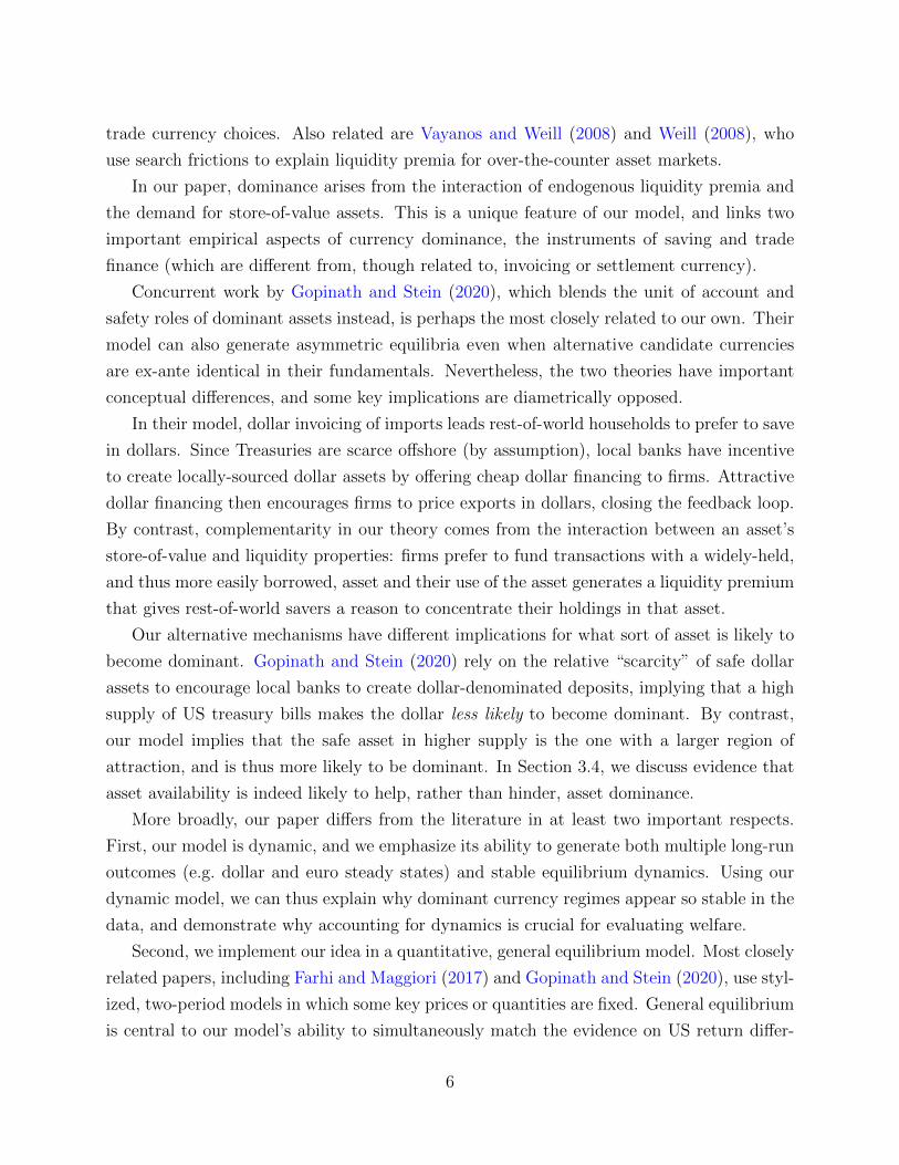
Concurrent work by Gopinath and Stein (2020), which blends the unit of account and

safety roles of dominant assets instead, is perhaps the most closely related to our own. Their

model can also generate asymmetric equilibria even when alternative candidate currencies

are ex-ante identical in their fundamentals. Nevertheless, the two theories have important

conceptual differences, and some key implications are diametrically opposed.

In their model, dollar invoicing of imports leads rest-of-world households to prefer to save

in dollars. Since Treasuries are scarce offshore (by assumption), local banks have incentive

to create locally-sourced dollar assets by offering cheap dollar financing to firms. Attractive

dollar financing then encourages firms to price exports in dollars, closing the feedback loop.

By contrast, complementarity in our theory comes from the interaction between an asset’s

store-of-value and liquidity properties: firms prefer to fund transactions with a widely-held,

and thus more easily borrowed, asset and their use of the asset generates a liquidity premium

that gives rest-of-world savers a reason to concentrate their holdings in that asset.

Our alternative mechanisms have different implications for what sort of asset is likely to

become dominant. Gopinath and Stein (2020) rely on the relative “scarcity” of safe dollar

assets to encourage local banks to create dollar-denominated deposits, implying that a high

supply of US treasury bills makes the dollar less likely to become dominant. By contrast,

our model implies that the safe asset in higher supply is the one with a larger region of

attraction, and is thus more likely to be dominant. In Section 3.4, we discuss evidence that

asset availability is indeed likely to help, rather than hinder, asset dominance.

More broadly, our paper differs from the literature in at least two important respects.

First, our model is dynamic, and we emphasize its ability to generate both multiple long-run

outcomes (e.g. dollar and euro steady states) and stable equilibrium dynamics. Using our

dynamic model, we can thus explain why dominant currency regimes appear so stable in the

data, and demonstrate why accounting for dynamics is crucial for evaluating welfare.

Second, we implement our idea in a quantitative, general equilibrium model. Most closely

related papers, including Farhi and Maggiori (2017) and Gopinath and Stein (2020), use styl-

ized, two-period models in which some key prices or quantities are fixed. General equilibrium

is central to our model’s ability to simultaneously match the evidence on US return differ-

6

entials, net foreign asset positions, and international financial adjustment documented by

Gourinchas and Rey (2007a,b), each of which have important welfare implications.

2 Simplified Model

In this section, we present a simplified version of our model that focuses on the two

essential ingredients of our mechanism: the savings decisions of households and the financing

decisions of firms. The simplified model allows us to characterize the key forces analytically,

and in Section 3, we explore quantitative implications in a rich general equilibrium setting.

The world consists of two symmetric big countries, the United States (US) and the

Eurozone (EZ), of equal size µus = µez, and a continuum of small open economies making

up the rest of the world (RW) with total mass µrw. There are two ex-ante identical assets –

a bond issued by the US government and a bond issued by the Eurozone government – each

recognized as safe and available in exogenous supply, B. Both assets serve as saving vehicles

and, potentially, as collateral guaranteeing international transactions.

Countries are indexed by j ∈ {us, ez, [0, µrw]} and within each country j, there is rep-

resentative consumer and a continuum of risk-neutral international trading firms. In the

simplified model, the only decision of the household is how to allocate its savings between

the two available assets and the only decision of a trading firm is which type of asset to seek

for financing its trade. We describe the decisions of the two agents types in turn.

Households

Households solve a standard consumption-savings problem, allocating their endowment

income between consumption and the two assets. In the simplified model, we assume there

is a single consumption good and both assets promise one unit of that good (we generalize

this later). Hence, bonds are ex-ante equivalent – however, as we will see, they may serve

different trade financing roles in equilibrium and, therefore, earn different interest rates.

Households in each country j ∈ {us, ez, [0, µrw]} solve

maxCjt,B

$jt,B

ejt

E0

∞∑t=0

βtC1−σjt

1− σsubject to

Cjt +Q$tB

$jt +Qet B

ejt = B$

jt−1 +Bejt−1 + ∆$jtB

$jt + ∆ejtB

ejt + Yjt,

and a non-negativity constraint on bond-holdings. In the above, Qct where c ∈ {$,e} is the

price of a US or Eurozone bond, Bcjt is the amount of that bond held by the household, and

7

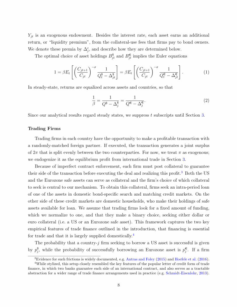
Yjt is an exogenous endowment. Besides the interest rate, each asset earns an additional

return, or “liquidity premium”, from the collateral-use fees that firms pay to bond owners.

We denote these premia by ∆cj, and describe how they are determined below.

The optimal choice of asset holdings B$jt and Bejt implies the Euler equations

1 = βEt

[(Cjt+1

Cjt

)−σ1

Q$t −∆$

jt

]= βEt

[(Cjt+1

Cjt

)−σ1

Qet −∆ejt

]. (1)

In steady-state, returns are equalized across assets and countries, so that

1

β=

1

Q$ −∆$j

=1

Qe −∆ej. (2)

Since our analytical results regard steady states, we suppress t subscripts until Section 3.

Trading Firms

Trading firms in each country have the opportunity to make a profitable transaction with

a randomly-matched foreign partner. If executed, the transaction generates a joint surplus

of 2π that is split evenly between the two counterparties. For now, we treat π as exogenous;

we endogenize it as the equilibrium profit from international trade in Section 3.

Because of imperfect contract enforcement, each firm must post collateral to guarantee

their side of the transaction before executing the deal and realizing this profit.3 Both the US

and the Eurozone safe assets can serve as collateral and the firm’s choice of which collateral

to seek is central to our mechanism. To obtain this collateral, firms seek an intra-period loan

of one of the assets in domestic bond-specific search and matching credit markets. On the

other side of these credit markets are domestic households, who make their holdings of safe

assets available for loan. We assume that trading firms look for a fixed amount of funding,

which we normalize to one, and that they make a binary choice, seeking either dollar or

euro collateral (i.e. a US or an Eurozone safe asset). This framework captures the two key

empirical features of trade finance outlined in the introduction, that financing is essential

for trade and that it is largely supplied domestically.4

The probability that a country-j firm seeking to borrow a US asset is successful is given

by p$j , while the probability of successfully borrowing an Eurozone asset is pej . If a firm

3Evidence for such frictions is widely documented, e.g. Antras and Foley (2015) and Hoefele et al. (2016).4While stylized, this setup closely resembled the key features of the popular letter of credit form of trade

finance, in which two banks guarantee each side of an international contract, and also serves as a tractableabstraction for a wider range of trade finance arrangements used in practice (e.g. Schmidt-Eisenlohr, 2013).

8

successfully borrows a unit of collateral, it pays a fee, r$ or re respectively, to the household

for the use of the asset and proceeds to trade in the international market. If the firm is not

successful in these credit markets, it continues on to trade using a “backup” funding plan

that still provides its chosen collateral, but absorbs all surplus from the transaction.5

The only equilibrium requirement for the funding fees r$ and re is that they leave firms

with a positive ex-post surplus. In parallel with the labor search literature, these prices can

be treated as parameters or they could be determined via some bargaining paradigm, which

can then be parameterized itself. For simplicity, we follow the first of these paths and fix

the funding prices to a common value, r$ = re = r < π.6

Once successfully funded, the firm is randomly matched with a trading counterparty

from another country j′ 6= j. Upon matching, the pair transacts using their collateral to

clear any payments needed and splits the gross transaction surplus of 2π. In the event that

the two counterparties’ collateral is mismatched — i.e. that one side of the match uses US

assets and the other side Eurozone assets as collateral — the transaction’s surplus is reduced

by a collateral mismatch cost of 2κ. Throughout, we assume that κ < π − r, so that the

transaction is profitable even in the event of a mismatch. This “collateral mismatch” cost can

be micro-founded as an expected cost in case of default, since having collateral denominated

in different currencies means two promises may not be equivalent in all states of the world.7

Putting everything together, a country-j firm chooses to apply for dollar trade financing

if the expected payoffs of seeking dollar financing is higher than seeking euro financing. The

differential payoff of seeking a US asset over a Eurozone asset is given by

V $j = p$

j

[π − r$

j − κ(1− X)]− pej

[π − rej − κX

], (3)

where X is the fraction of all trading firms in the world that use dollar funding and, hence,

the probability an individual firm matches with a counterparty that uses dollar financing.

Naturally, firms prefer to use dollar financing so long as V $j > 0.

Since our primary aim is to explain third-party use of a dominant currency, we assume

that firms in the US and Eurozone always seek to be funded via their respective domestic

assets, and solve for the optimal currency choice of the rest-of-world trading firms.8 Under

5This assumption simplifies derivations; in our quantitative model, unfunded firms exit without trading,so that trade finance constitutes a real constraint on equilibrium trade flows.

6Nash bargaining with an appropriate choice of bargaining parameter gives identical results.7Note that our results require that κ is not too big, which would explain why it is not hedged away.8An earlier version of the paper, Chahrour and Valchev (2017), considered endogenous funding choices for

the US and the Eurozone and arrives at very similar conclusions, at the cost of complicating the exposition.

9

these assumptions, the average use of dollar trade financing around the world is

X ≡ µusXus + µezXez +

∫ µrw

0

Xjdj = µus +

∫ µrw

0

Xjdj,

where Xj is the fraction of firms in country j ∈ [0, µrw] that apply for dollar financing.

We assume that the number of matches in a given country-asset credit market is governed

by the constant returns to scale den Haan et al. (2000) matching function

MF (B,X) =BX

B +X,

where B represents units of the asset on offer and X, the number of trading firms demand-

ing that asset. For example, a country-j firm searching for dollar funding succeeds with

probability

p$j =

MF (B$j , Xj)

Xj

=B$j

B$j +Xj

.

Substituting expressions for the funding probabilities into equation (3) yields

V $j =

B$j

B$j +Xj

[π − r − κ(1− X)

]−

BejBej + 1−Xj

[π − r − κX

]. (4)

Equation (4) reveals the individual firm’s three strategic incentives, two with respect to

other trading firms and one with respect to the domestic household. First, with respect to

other domestic firms, collateral choices are strategic substitutes : when a larger share of the

other country-j traders apply for dollar funding (higher Xj), the local dollar funding market

becomes more congested, lowering the probability a given trader’s dollar loan is approved,

thus lowering the relative payoff of seeking this type of funding.

Second, funding choices with respect to foreign trading firms (X), are strategic com-

plements due to collateral mismatch costs. This complementarity can lead to a standard

type of sunspot multiplicity, in which both dollar or euro use can be sustained as equilibria,

depending on the conjecture of X.

The third strategic interaction occurs between between the collateral choice of trading

firms and the savings choices of households. Equation (4) captures this interaction via the

presence of B$j and Bej in the funding probability terms. For example, a trading firm’s ex-

pected payoff of seeking dollar financing increases with the household’s holdings of US bonds

(B$j ), as larger household US asset holdings increase the firm’s probability of successfully ob-

taining dollar funding.

10

This final strategic interaction works against sunspot equilibria: the funding friction

makes households’ bond positions a coordination device, anchoring firms’ expectations of

others’ choices to credit market conditions. To analyze this formally, we define a quasi-

equilibrium in trade finance use, in analogy to Mas-Colell et al. (1995, p. 551). We focus on

symmetric equilibria in which Xj = Xrw, B$j = B$

rw, and Bej = Berw for all j ∈ [0, µrw].

Definition 1 (Quasi-equilibrium). Given household asset holdings in rest-of-world coun-

tries {B$rw, B

erw}, a symmetric quasi-equilibrium in funding choice is a rest-of-world traders’

funding choice Xrw such that no trader has an incentive to change its trade finance choice.

Quasi-equilibrium describes the equilibrium funding choice among trading firms as a

function of the asset holdings of the households and we denote the set of quasi-equilibria

by the correspondence X(B$rw, B

erw). Using equation (4), the set of quasi-equilibria can be

characterized by the condition

V $Xrw(1−Xrw) = 0, (5)

with V $ > 0 only if Xrw = 1 and V $ < 0 only if Xrw = 0. If there is a unique value of Xrw

satisfying (5), then X(B$rw, B

erw) becomes a function.

Lemma 1 characterizes some key properties of the quasi-equilibria in our economy:

Lemma 1. Given household portfolio holdings, the currency quasi-equilibrium is unique for

any feasible bond allocation if and only if

κ < κsunspot ≡ π − rB + µrw

2+ 1

2

.

In that case, X(B$rw, B

erw) ∈

[max{B$

rw,Berw}

B$rw+Berw

, 1].

Proof. Proved in Appendix A. �

Lemma 1 shows that the quasi-equilibrium funding choice can be unique even when

there are strategic complementarities across countries (i.e. κ > 0). This happens because

credit market conditions affect the accessibility of funding for firms’ counterparties and the

chief determinant of that accessibility is the household portfolio position. As a result, bond

holdings can become a coordination device that uniquely synchronizes trade finance choices

on the asset that forms a higher proportion of rest-of-world portfolios.

Naturally, if we reduce the effective financial friction, for example by raising both B$rw and

Berw which makes both types of funding easier to obtain and reduces the congestion effects

in credit markets, the scope for indeterminacy increases and the threshold κsunspot falls.

11

In fact, if asset holdings of both types become arbitrarily large, potential counterparties’

choices become the only payoff-relevant factor in the funding choice of firms and the quasi-

equilibrium is not unique for any level of κ:

Corollary 1. In the limit of B$rw →∞ and Berw →∞, for any κ > 0

X(B$rw, B

erw)→ {0, 1/2, 1}.

We refer to indeterminacy in the funding choice quasi-equilibrium as “sunspot” multi-

plicity, because in that case the funding choices are solely determined by the beliefs of what

other trading firms would do, i.e. a sunspot shock in the expectations of others’ actions.

Next, we characterize the effects of firm funding decisions on household savings choices.

The holding premium earned by a bond is equal to the expected intra-period loan fees that

the bond earns. These fees are just the probability that a country j household successfully

lends this kind of bond times the funding fee r that it receives when it does so. Hence,

∆$j =

MF (B$j , Xj)

B$j

× r =Xj

B$j +Xj

r, (6)

∆ej =MF (Bej , 1−Xj)

Bej× r =

(1−Xj)

Bej + (1−Xj)r. (7)

Since the Euler equation (2) holds for all households j, the liquidity premia earned by

each asset are equalized across countries: ∆cj = ∆c for all j ∈ {us, ez, [0, µrw]}. Using

this observation, the Euler equations, and the market clearing conditions in bond markets

(µusBcus + µezB

cez +

∫Bcjdj = B), we can derive Lemma 2.

Lemma 2. Equilibrium household portfolios, as a function of traders’ currency choices, are:

B$j = B

Xj∫ µrw0

Xjdj + µus(8)

Bej = B1−Xj∫ µrw

0(1−Xj)dj + µez

. (9)

Proof. Proved in Appendix A. �

Lemma 2 describes the equilibrium household portfolios as a function of the mix of assets

used for trade financing by firms. This relationship is upward sloping: higher Xj implies

higher B$j . Intuitively, an asset that is heavily used for funding international transactions

will deliver a higher liquidity premium ceteris paribus, increasing households’ incentive to

12

hold that bond. Since bond premia are equalized across countries, countries with a higher

dollar usage (higher Xj) must also have higher portfolio holdings of US bonds (B$j ).

Together, Lemmas 1 and 2 summarize the strategic firm-household interaction that is

both novel and central our mechanism: Higher holdings of a given asset by rest-of-world

households tilt the quasi-equilibrium in funding choices towards that asset, while use of the

asset in funding markets reinforces the rest-of-world households’ decision to save in it.

Steady-state equilibria

Having characterized both the financing choices of firms and the savings choices of house-

holds, we now analyze steady-state equilibria. We consider symmetric steady states in which

the strategies of the ex-ante identical rest-of-world agents are the same.

Definition 2. A steady-state equilibrium is a rest-of-world currency usage Xrw, a set of asset

holdings {B$rw, B

erw, B

$us, B

eus, B

$ez, B

eez}, bond prices {Q$, Qe} and premia {∆$,∆e} such that

1. There is a quasi-equilibrium in currency choice.

2. The optimality conditions of household bond holdings are satisfied.

3. Bond markets clear:

B = µrwBcrw + µusB

cus + µezB

cez, for c ∈ {$,e}.

4. The bond liquidity premia equal fees paid by firms as per equations (6) and (7).

Proposition 1 summarizes the characteristics of the emerging steady-state equilibria.

Proposition 1. For any κ ≥ 0, the economy has three steady-state equilibria:

(i) a dollar-dominant steady state with Xrw = 1 and Berw = 0;

(ii) a euro-dominant steady state with Xrw = 0 and B$rw = 0; and

(iii) a multipolar steady state with Xrw = 1/2 and B$rw = Berw.

Outside of the knife-edge case where κ = π−rB+1

, these are also the only steady states.

Proof. Proved in Appendix A. �

13

Crucially, each steady-state is jointly characterized by a specific rest-of-world savings

composition and a corresponding trade finance choice. For example, at the dollar-dominant

steady state, the rest-of-world holds large amounts of the US asset, making dollar financing

the most convenient for their firms, reinforcing their trade finance choices. The rest-of-world

households, in turn, are happy to concentrate their savings in US assets because the demand

for dollar funding supports a liquidity premium on US assets.

This logic also explains why steady-state multiplicity is robust to generalizing many

of the details in our model. For example, any strategy that traders may take to avoid

paying currency mismatch costs — such as directing their search to counterparties holding

a particular type of collateral or renegotiating the settlement currency ex-post — will not

eliminate the interaction between households and firms. Similarly, the result is robust to

allowing households to lend their assets as collateral in foreign markets, since the optimal

allocation of assets across credit markets in each country j must still satisfy (8) and (9).9

Stability of steady states

One of our main objectives is to understand why dominant-asset regimes appear to be so

stable in the data. We have already shown that, when κ < κsunspot, sunspot shocks cannot

change the equilibrium in trade finance markets, given household asset positions. We now

derive the conditions under which the interaction between households and firms results in

locally stable dominant-asset steady states, in the sense that the best response functions

of both agent types jointly define a local contraction map. Intuitively, we want to ensure

that deviations in saving or trade finance choices would not unravel the dominant asset

equilibrium.

Proposition 2 shows that the model with intermediate values of κ can generate dominant-

asset steady states that are both locally stable and not subject to sunspot shocks.

Proposition 2. For κ > κ the dominant-currency steady states are locally stable, where

κ ≡ π − rB + 1

< κsunspot.

Proof. Proved in Appendix A. �

The result is due to the interaction among the incentives trading firms face in their financ-

ing choice, the differential availability of financing due to the feedback between households

9This would be akin to global banks being active in many trade finance markets through country-specificbureaus. While the model is robust to this, our benchmark assumption that trade finance is domesticallysourced in rest-of-world countries is consistent with the BIS (2014) data for emerging markets.

14

and firms, and the cross-country coordination incentive among trading firms.

To see how these forces interact, consider a situation in which the economy begins at the

dollar-dominant steady state, with rest-of-world household portfolios concentrated in US as-

sets and rest-of-world firms using only US safe assets for financing their trade. Suppose now

that households shift their savings a little towards Eurozone assets. The increased availabil-

ity of euro financing gives firms an incentive to shift towards funding via Eurozone assets.

However, as long as κ > κ, firm choices will not change much: the small shift in portfolios still

leaves dollars the most widely available in world markets and, hence, firms still coordinate

strongly on dollars. Thus, for a local shift in household portfolios, the cross-country coor-

dination of firms prevents the currency quasi-equilibrium (X) from changing significantly,

which in turn means that the conjectured shift in household portfolios is suboptimal.

Proposition 2 implies there is a range of parameter values over which dominant asset

steady states are both locally stable and not subject to sunspot shocks.

Corollary 2. There exist a non-empty range, κ ∈ (κ, κsunspot), over which the dominant-

asset steady states are both locally stable and not subject to sunspot shocks.

The existence of this region depends crucially on the interaction of our two complemen-

tarity forces: Currency sunspots require coordination incentive across firms to be so strong

that a unilateral deviation in trade finance choice can be sustained, even given fixed portfo-

lios. By contrast, local stability requires intermediate-strength coordination incentives, such

that firms will only deviate from a dominant asset equilibrium if households also dramati-

cally change their portfolio composition. Hence, necessarily, κ < κsunspot. By the same logic,

neither the asset availability mechanism nor cross-country complementarity can achieve such

stability on their own: If κ = 0, dominant-asset steady states are unstable, while if κ > 0

and bond supplies are infinite (so credit frictions are non-existent), the firms’ funding choices

are subject to sunspot shocks. We illustrate this argument graphically in Appendix B.

3 Dynamic General Equilibrium Model

Having illustrated the key intuition of our mechanism, we now embed it in a rich dynamic

general equilibrium model. We calibrate the model, and show it can match both targeted and

untargeted moments, quantify the welfare effects of dominance, and perform counterfactuals

to better understand the conditions under which dominant currencies can fall.

15

3.1 Setup

Like our stylized model, our general environment consists of households and firms in the

US, Eurozone, and a continuum of rest-of-world small open economies, but each of those

agents now has several margins of choice. Households choose a basket of consumption, as

well as their optimal savings patterns. Trading firms make optimal choices about whether

to operate and how/where to trade, as well as the choice of how to finance their activities.

Finally, all prices and quantities are determined in general equilibrium.

3.1.1 Households

In each country j ∈ {us, ez, [0, µrw]}, a representative household seeks to maximize the

present discounted value of utility of consumption, E0

∑∞t=0 β

t C1−σjt

1−σ . In contrast to Section 2,

there are country-specific differentiated goods, and the consumption basket Cjt is a Cobb-

Douglas aggregate of all domestic and foreign goods. The consumption share of the domestic

good is ah ∈ (0, 1), and the consumption shares for foreign goods are proportional to the

size of their origin country. For example, the US consumption basked is

Cus,t = (Cusus,t)

ah(Cezus,t)

(1−ah)µezµez+µrw (Crw

us,t)(1−ah)µrwµez+µrw . (10)

In the above, Cijt denotes consumption of good i in country j and Crw

jt ≡ (∫ µrw

0(Ci

jt)η−1η di)

ηη−1

aggregates goods from the small open economies.10 The consumption baskets of the Eurozone

and rest-of-world economies are analogous and presented in the Online Appendix.

Because of the frictions in international trade, the law of one price does not hold in our

economy and goods have different equilibrium prices in different locations, with a markup

on imports P ij,t > P j

j,t. This markup relative to the origin-country price is endogenous and

depends on the equilibrium patterns of trade, as we describe below. Nevertheless, since our

economy is real, all prices can be expressed in terms of a numeraire good, which we take as

the (identical) domestic price of the small open economy goods, i.e. P rwrw,t ≡ 1.

In addition to consumption, households choose how much to save and how to allocate

savings among US and Eurozone bonds, each of which yields a risk-free unit of their respective

domestic good. The household in country j faces the budget constraint:

PjtCjt + (1−∆$jt)P

usus,tQ

$tB

$jt + (1−∆ejt)P

ezez,tQ

et Bejt + adj. costst

10The price index corresponding to (10) is Pus,t = K−1(Pusus,t)

ah(P ezus,t)

(1−ah)µezµez+µrw (P rw

us,t)(1−ah)µrwµez+µrw , where K

is a proportionality constant and P jus,t is the price of country j’s differentiated good in the US.

16

= P usus,tB$jt−1 + P ezez,tB

ejt−1 + P jjtYjt + ΠT

jt + Tjt, (11)

where Q$t and Qet are the prices of the US and the Eurozone bonds, Yjt is the household’s

endowment of its domestic good, ΠTjt is the total profit of country j’s import/export firms

(described below), and Tjt are lump-sum taxes. As in our simple model, a household’s bond

holdings earn an endogenous liquidity premium, given by the intra-period cash flows ∆$jt and

∆ejt. We focus on a perfect foresight, symmetric model and assume that all endowments are

constant through time and equal, Yjt = Y for all j.

Households are also subject to external portfolio adjustment costs, given by

adj. costst ≡ P usus,tQ

$t τ(B$

jt, B$j,t−1) + P ez

ez,tQet τ(Bejt, B

ej,t−1).

These costs are parameterized by the function τ(B,B) ≡ τ2

(B−BB

)2

B, which is quadratic in

terms of percent deviations from the country-wide bond holdings entering the period, B$j,t−1

and Bej,t−1. These adjustment costs are zero at (any) steady state, and thus have no effect

on steady states, but serve to limit the volatility of capital flows outside of steady state.

Intertemporal optimality implies the following household Euler equation for dollar bonds

1 = βEt

(Cjt+1

Cjt

)−σPjtPjt+1

P usus,t+1

P usus,t

1

Q$t

(1−∆$

jt + τ ′(B$jt, B

$j,t−1)

) . (12)

This equation is same as (1), except that it now reflects the consequences of relative price

differences among goods and across time, as well as the influence of adjustment costs on

effective bond returns. An equation that is analogous to (12) holds for euro bond holdings.

3.1.2 The Import-Export Sector

International goods trade is subject to search and matching frictions as emphasized by the

recent trade literature (e.g. Antras and Costinot, 2011). International trade flows through

specialized import/export firms, who organize to sell country-j’s differentiated good in coun-

try i, via a match between a country-j export firm with a country-i import firm.

Once matched, the exporting firm buys goods at the prevailing domestic market price

and sells them to the matched foreign importer, who then resells the good to the country-

i household at the prevailing market price in that location. Firms optimally choose the

intensity with which they search for different types of trade partners (e.g. import from US

vs. import from the Eurozone), and the resulting matching patterns determine the size and

17

direction of equilibrium trade flows. The import/export firms operate within the period,

return profits to households, and disband.11

As before, international trade is subject to a financial friction, which implies a need for

trade finance. Firms look for a fixed amount of funding, which we normalize to one unit of

the numeraire, and firms again make the binary choice of either seeking US or Eurozone safe

assets. Both of these assumptions can be relaxed.

A trading firm’s choices occur in two stages. In the first, the firm chooses whether or

not to pay a fixed cost and become operational in a given period and the likelihood that,

if operational, it will pursue an import or an export opportunity and with which partner

country. Second, the firm chooses the type of trade financing to apply for. We consider each

stage in detail before characterizing equilibrium in the model.

Entry and trading pattern choice

Trading firms pay a fixed cost φ in units of their domestic good to enter the international

trade market. Thus, a firm enters only if the expected profits from trading net of this cost

are positive, and the ones that do enter make a probabilistic choice regarding the direction

in which they will trade. Specifically, an active country-j firm chooses the probabilities with

which it will become an importer from country i or an exporter to country i, for all i, which

probabilities we denote pimjit and pexjit respectively. In equilibrium, the pattern is such that

firms are indifferent between operating as an importer or exporter in any direction. We

provide a detailed description of the firm’s entry decision in the Online Appendix.

Funding Choice

As in the analytical model, trading firms must arrive to international trade markets

with either US or Eurozone safe asset collateral, which they borrow from their domestic

households through bond-specific search and matching markets.

Relative to the analytical model in Section 2, we enrich our model of trade finance supply

in a two ways. First, we tie the potential liquidity service of an asset to the total market

value of the household’s holdings of that asset. Second, because we will calibrate our model

to annual data while the typical trade finance arrangement is much shorter, we introduce

a parameter ν that corresponds to the number of times a given bond could be used to

intermediate trade within one model period. Thus, the total value of trade flows that the

11This assumption aligns well with evidence of high churn in firm-to-firm trade relationships (Eaton et al.,2016).

18

country j holdings of US and Eurozone safe assets can intermediate is given by νP usus,tB

$jtQ

$t

and νP ezez,tB

ejtQ

et respectively, the market value of holdings scaled up by ν.

With these assumptions, the probability of success faced by a country-j trading firm

seeking US financing is

p$jt =

MF(mjtXjt, νP

usus,tB

$jtQ

$t

)mjtXjt

= MF

(1,νP us

us,tB$jtQ

$t

mjtXjt

), (13)

where mjt is the total mass of operational country-j firms, as determined by the zero-profit

entry condition, and thus mjtXjt is the mass of country-j firms applying for dollar funding.

Note that we also use the general form of the den Haan et al. (2000) matching function

MF (u, v) = uv

(u1ξF +v

1ξF )ξF

, which allows for an elasticity parameter εF that we calibrate to

the data. The probability a country-j trading firm seeking Eurozone bonds finds a credit

match, pejt, is given by an analogous expression.

In sum, the market tightness of each trade finance market is given by ratio of supply to

demand in each:νPusus,tB

$jtQ

$t

mjtXjtand

νP ezez,tBejtQ

et

mjt(1−Xjt) . We note here that tying the effective trade finance

supply to the market value of assets introduces a new channel that generally reinforces the

emergence of a dominant asset: Since a dominant asset carries a high equilibrium price, an

asset’s ability to facilitate trade increases as it becomes dominant.

As in Section 2, we fix the collateral use in the big countries exogenously, though now

we calibrate Xus = 1 − Xez to the domestic-currency trade finance usage in the US and

Eurozone data, which is high but not exactly 100%. We continue to assume that the US and

Eurozone firms face the same financing frictions as small open economies, so equation (13)

and its euro analogue apply without modification for these countries as well.

In making their funding choices, rest-of-world firms compare the respective expected

profits of seeking dollar and euro financing. Upon a successful funding match, the expected

profit of a country-j trading firm using US safe assets as a collateral guarantee is given by

Π$jt =

∑i 6=j

pimjitπ$,imjit +

∑i 6=j

pexjitπ$,exjit ,

where π$,imjit is the expected profit of a firm importing from i to j that is financed via US

bonds, and π$,exjit is the analogous values for a country-j exporter looking to match with

a country-i importer. The corresponding expected profits of a country-j firm funded with

Eurozone assets, Πejt is analogous. We describe the determinants of trading profits below.

In return for the intra-period use of the household’s bonds, the firm pays a fee r. Thus,

19

the expected net payoff to a country-j firm of seeking dollar funding is then given by

Π$jt = p$

jt(Π$jt − r), (14)

which is simply the probability of obtaining dollar funding, p$jt, times the expected profit net

of the dollar funding costs. The expected payoff to seeking euro funding is Πejt = pejt(Πejt−re).

Lastly, to match the empirical fact that, despite its dominance, the dollar is not the

only currency used to finance global trade, we introduce an i.i.d. additive idiosyncratic

preference shock for the type of trade financing a firm l prefers, all else equal, θ(l)jt ∼ N(0, σ2

θ).

This generates some idiosyncratic heterogeneity across firms and thus results in an interior

equilibrium value for the currency mix Xjt, which we can then calibrate to the data.

Combining the probabilities of obtaining each type of funding, the expressions for profits,

Π$jt and Πejt, and the disturbance θ

(l)it , we can compute an individual firm’s net benefit of

seeking financing via US assets:

V$,(l)jt =

1[1 + (

mjtXjt

νPusus,tB$jtQ

$t

)1ξF

]ξF (Π$jt − r)−

1[1 + (

mjt(1−Xjt)νP ezez,tB

ejtQ

et)

1ξF

]ξF (Πejt − r) + θ(l)it .

Firm l in country j will then choose to seek dollar funding if and only if V$,(l)jt > 0. Given

that the expected payoff of seeking dollar funding is increasing in θ(l)jt , we can express the

optimal choice in terms of a threshold strategy, where the firm seeks dollar funding if and

only if their idiosyncratic shock exceeds a country-specific threshold θjt. Thus, the fraction

of country-j trading firms using US safe assets is

Xjt =

∫ 1

0

1(θ(l)jt >= θjt)dl = 1− Φ

(θjtσθ

),

where Φ(·) denotes the standard normal CDF.

In equilibrium, the cutoff θjt is defined by V$,(l)jt = 0, the value of the idiosyncratic

preference shock that leaves a country-j firm indifferent between choosing one asset or the

other. We focus on symmetric equilibria where all ex-ante identical rest-of-world countries

have the same equilibrium allocations, hence θjt = θt for all j ∈ [0, µrw].

Exchange of Goods

Firms that are successful in obtaining financing then discover whether they will import

or export, and from/to where, according to the probabilities pimjit and pexjit that they chose

20

optimally upon entry. Country-j exporters match with country-i importers according to the

technology MT (u, v) = uv

(u1εT +v

1εT )εT

, which is of the same functional form as the matching

function in credit markets, but allows for a different elasticity parameter εT .

The probability of a country-j exporter matching with a country-i importer is

peijit =MT

(mexjit, m

imijt

)mexjit

=(

1 +(mexjit/m

imijt

)1/εT)−εT

.

where mimijt = pimijtmit(p

$itXit + peit(1−Xit)) is the mass of funded importing firms in country

i seeking trade with country-j firms that are looking to export to i, which are themselves of

mass mexjit = pexjitmit(p

$itXit + peit(1−Xit)). Using analogous derivations, the probability of a

country-j importer matching with a country-i exporter is piejit =(

1 +(mimjit/m

exijt

)1/εT)−εT

.

In a successful match between a country-j exporter and a country-i importer, the exporter

buys the j good at its domestic market price P jjt and the importer then sells it to the country-i

household at the prevailing market price in that location P jit. The transaction thus generates

a gross surplus of P jit − P

jjt, which is then also subject to a collateral mismatch cost κ.

The importer and exporter in a trading match split the surplus of their transaction via

Nash bargaining, with the exporter having a Nash bargaining share of α. The effective

“wholesale” price at which a country-j exporter sells to a country-i importer is thus Pwholjit =

P jjt + α(P j

it − Pjjt). The expected profit of a firm looking to export from country j to i is

π$,exjit = peijit

α

Pwholjit

[P jit − P

jjt − κPwhol

jit (1− Xit)]. (15)

The term in square brackets is the net expected surplus per unit of goods traded, which

is given by the gross markup on the imported good, net of the expected currency mismatch

cost κPwholjit (1− Xit). In this expression,

Xit ≡p$itXit

p$itXit + peit(1−Xit)

is the average use of dollar trade financing among the funded country-i firms (which are thus

actively searching for trade counterparts), hence 1− Xi,t is the probability of matching with

a EUR-funded country-i importer, and thus having to incur the expected default cost κ.12

12Note that since a potential trading partner’s funding is uncertain, it would be costly to first match witha counterparty, agree on a particular type of collateral, and only then seek that financing. If the financingfalls through, the firm looses the opportunity to earn π, which is simply not worth the risk for potentiallysaving the small mismatch cost κ.

21

Lastly, the financing friction limits the overall value of the transaction to the value of

the attached safe collateral. Since we assume each firm borrows one numeraire unit of safe

assets, to obtain the net expected profit from the view point of a country-j exporter (who

earns α fraction of the total surplus), the expected per-unit profit is then scaled by αPwholjit

.

Government

We assume that government purchases are zero, and thus governments play a role only in

the large countries j ∈ {us, ez}, where they issue bonds in fixed supply B = B$ = Be and set

the level of lump-sum taxes so as to keep their stock of debt constant, so that B = Tjt+QjtB.

The small rest-of-world countries j ∈ [0, µrw] do not issue debt and set Tjt = 0.

Equilibrium

In equilibrium, the liquidity premia a country-j household can earn on lending US and

Eurozone bonds respectively are equal to the frequency with which the household successfully

lends the asset in its respective credit market multiplied by the funding fee r:

∆$jt =

νmjtXjt[(mjtXjt)

1/ξF + (νP usus,tB

$jtQ

$t )

1/ξF

]ξF r (16)

∆ejt =νmjt(1−Xjt)[

(mjt(1−Xjt))1/ξF + (νP ez

ez,tBejtQ

et )1/ξF

]ξF r (17)

Given those expressions, the rest of the equilibrium is determined by the household and

firms’ optimal decisions, and market clearing in real goods and bond markets. We focus on

the class of symmetric equilibria where the strategies of the ex-ante identical rest-of-world

trading firms and households are the same, e.g. Xjt = Xrw,t for all j ∈ [0, µrw]. A complete

definition of equilibrium is provided in the Online Appendix.

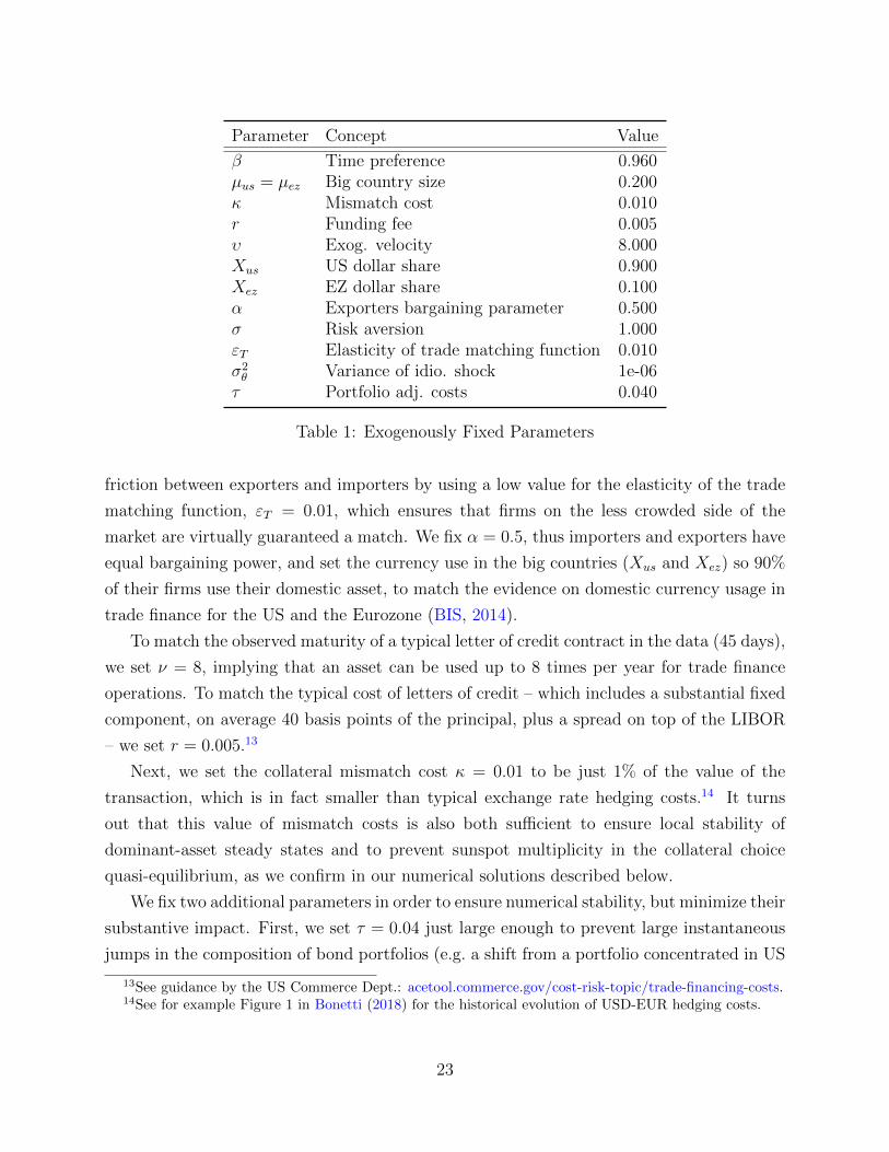
3.2 Calibration

We fix a set of parameters to standard values, then use the remaining parameters to

target several moments, which the model replicates exactly. Table 1 lists the exogenously-

fixed parameters. Specifically, we set µus = µez = 0.2, consistent with the sizes of the

US and the Eurozone in world GDP. One model period represents a year, hence we set

β = 0.96; we also assume log preferences (σ = 1). Next, we minimize the role of the search

22

Parameter Concept Value

β Time preference 0.960µus = µez Big country size 0.200κ Mismatch cost 0.010r Funding fee 0.005υ Exog. velocity 8.000Xus US dollar share 0.900Xez EZ dollar share 0.100α Exporters bargaining parameter 0.500σ Risk aversion 1.000εT Elasticity of trade matching function 0.010σ2θ Variance of idio. shock 1e-06τ Portfolio adj. costs 0.040

Table 1: Exogenously Fixed Parameters

friction between exporters and importers by using a low value for the elasticity of the trade

matching function, εT = 0.01, which ensures that firms on the less crowded side of the

market are virtually guaranteed a match. We fix α = 0.5, thus importers and exporters have

equal bargaining power, and set the currency use in the big countries (Xus and Xez) so 90%

of their firms use their domestic asset, to match the evidence on domestic currency usage in

trade finance for the US and the Eurozone (BIS, 2014).

To match the observed maturity of a typical letter of credit contract in the data (45 days),

we set ν = 8, implying that an asset can be used up to 8 times per year for trade finance

operations. To match the typical cost of letters of credit – which includes a substantial fixed

component, on average 40 basis points of the principal, plus a spread on top of the LIBOR

– we set r = 0.005.13

Next, we set the collateral mismatch cost κ = 0.01 to be just 1% of the value of the

transaction, which is in fact smaller than typical exchange rate hedging costs.14 It turns

out that this value of mismatch costs is also both sufficient to ensure local stability of

dominant-asset steady states and to prevent sunspot multiplicity in the collateral choice

quasi-equilibrium, as we confirm in our numerical solutions described below.

We fix two additional parameters in order to ensure numerical stability, but minimize their

substantive impact. First, we set τ = 0.04 just large enough to prevent large instantaneous

jumps in the composition of bond portfolios (e.g. a shift from a portfolio concentrated in US

13See guidance by the US Commerce Dept.: acetool.commerce.gov/cost-risk-topic/trade-financing-costs.14See for example Figure 1 in Bonetti (2018) for the historical evolution of USD-EUR hedging costs.

23

Concept Data Model

Gross debt/GDP 0.60 0.60ROW trade/GDP 0.55 0.55ROW USD usage 0.80 0.80Import markup 1.10 1.10

(a) Calibration Targets

Parameter Concept Value

B US/EZ asset supply 1.471ahj Home bias 0.718

εf Funding match. elas. 0.294φ Fixed cost of entry 0.038

(b) Implied Parameter Values

Table 2: Calibration Strategy

asset, to one concentrated in Eurozone assets within a period) that could lead to equilibrium

multiplicity. This value implies that a 10% change in bond positions incurs a cost of just

2 basis points on the portfolio. We also make the currency preference shocks as small as

possible (σ2θ =1e-06), while still ensuring numerically reliable interior solutions for Xrw.

We calibrate the remaining parameters to match a set of target steady-state moments.

Like our analytical model, the calibrated model has three co-existing steady states – dollar

and euro dominant ones, and a symmetric one. Since the dollar has long been the dominant

currency, we match the empirical moments from the past four decades to those at the dollar-

dominant steady state of the model. Panel (a) of Table 2 summarizes the targeted moments:

(1) government debt of 60% of GDP, consistent with the US average; (2) rest-of-world trade

share ( Imports + ExportsGDP

) of 55%, consistent with trade data for non-US and non-Eurozone

countries from the World Bank; (3) dollar share in trade financing used by rest-of-world

trading firms of 80%, consistent with the evidence on the fraction of letters of credit and

trade finance loans denominated in dollars BIS (2014); and (4) import markups of 10%,

consistent with micro-level estimates on import markups in Cosar et al. (2018).

We target these four moments with the four remaining free parameters {B, ah, εF , φ}.These parameters are: (1) the supply of government debt B; (2) the home bias parameter in

consumption preferences ah which determines the trade share; (3) the elasticity of the funding

matching function εF which helps determine the equilibrium level of currency coordination;

and (4) the fixed cost of entry in the trading sector φ which helps determine import markups.

We find the model can exactly match the targeted moments, with the implied parameter

values given in Panel (b) of Table 2.

3.3 Quantitative Results

We now consider the model’s quantitative implications for non-targeted moments in

steady-state and then proceed to use global techniques to solve for the model’s (perfect-

24

foresight) transition dynamics. We then explore the model’s implications for three counter-

factual scenarios. In the first, we examine what could have happened to dollar dominance

had the Eurozone continued it expansion beyond its current size. In the second, we explore

the implications of the decreasing relative size of the US compared to the world economy.

Finally, we explore potential consequences of trade wars initiated by the United States.

Steady State

Table 3 summarizes several key steady state moments in the calibrated economy, and

shows that the (empirically-relevant) dollar-dominant steady state matches a number of

untargeted phenomena. First, since the rest-of-world countries primarily use dollars for trade

finance (Xrw = 0.8), the US bond earns a higher equilibrium liquidity premium: ∆$ > ∆e,

which in turn results in an interest parity violation: Interest rates on Eurozone bonds must

exceed rates on US bonds in order to offset the lower liquidity return. Specifically, we find

1

Qe− 1

Q$=

∆$ −∆e

β= 1.07%,

which implies the US earns a significant “exorbitant privilege”. The size of this excess return

is consistent with the Gourinchas and Rey (2007a) evidence on exorbitant privilege and the

US Treasury convenience yield estimated by Jiang et al. (2020).

The third line of the table (seignorage) provides a common and simple estimate of the

net benefit the US receives from the “privilege” of this interest differential. This number is

computed as the counter-factual additional debt servicing payments the US would face if it

actually paid an interest rate equal to the inverse of the time discount, holding asset positions

constant. Essentially, this is the seignorage the US earns from the liquidity premium on its

asset and, at 0.88% of GDP, our model estimates this to be substantial.

Though similar calculations have often been used to estimate the benefits of exorbitant

privilege, our model implies that this is an incomplete and potentially misleading measure

of privilege because it takes asset positions as given. A key insight of our theory is that

widespread foreign holdings of a country’s assets are necessary to support its dominant

status. But such strong external demand leads to a negative steady-state net foreign asset

position for the central country, and hence the seignorage benefits of being dominant are at

least partially offset by the need to service the resulting negative net foreign asset position.

Indeed, the fourth line in the table shows that the dominant country (i.e. US) has a

significant negative net foreign asset position equal to -42% of GDP, while the other big

25

USD Dominant Multipolar EUR DominantMoments US EZ RW US EZ RW US EZ RW

Panel A: Benchmark model

USD share trade fin. (Xj) 0.90 0.10 0.80 0.90 0.10 0.50 0.90 0.10 0.20

100×(i$ − ie) 1.07 - - 0.00 - 0 - - -1.07 -100×Seignorage/GDP 0.88 0.23 - 0.56 0.56 - 0.23 0.88 -

NFA/GDP -0.42 -0.26 0.18 -0.38 -0.38 0.19 -0.26 -0.42 0.18Gross Foreign Assets/GDP 0.04 0.02 0.18 0.02 0.02 0.19 0.02 0.04 0.18100×Trade bal./GDP 0.87 0.86 -0.45 1.01 1.01 -0.52 0.86 0.87 -0.45

Panel B: Rest-of-World asset (Brw/(PrwY ) = 0.40)

100×(i$ − ie) 1.03 - - 0.00 - - - -1.03 -

NFA/GDP -0.14 0.01 0.03 -0.10 -0.10 0.05 0.01 -0.14 0.03Gross Foreign Assets/GDP 0.31 0.29 0.18 0.30 0.30 0.20 0.29 0.31 0.18100×Trade bal./GDP -0.25 -0.28 0.14 -0.12 -0.12 0.07 -0.28 -0.25 0.14

Table 3: Steady-state values for baseline model.

country (i.e. Eurozone) has a much better net foreign asset position of -26% of GDP. This

is a manifestation of the fact that rest-of-world households concentrate their savings in US

assets, which is the second sense in which those assets are dominant. In particular, the model

implies that two-thirds of rest-of-world portfolios are invested in US bonds, amounting to a

long position in US assets equal to 12% of rest-of-world GDP, consistent with the evidence

in Caballero et al. (2008). Overall, at our calibration the US trade balance is only slightly

better than that of the Eurozone, despite the excess return the US earns, suggesting that the

net welfare effect of dominance is small (which we quantify precisely later) since its position

as an external net debtor largely offsets the benefits of exorbitant privilege.

Lastly, we emphasize that while the US trade balance is positive in the benchmark model,

our mechanism can indeed generate a negative net foreign asset position and a trade deficit

at the same time. To illustrate this, Panel B of Table 3 considers a version of the model with

a richer asset structure, in which each of the small economies also issues government debt

equal to 40% of their GDP. The assets from each small country are measure zero, and hence

do not finance international trade, but households in all countries may hold the basket of

26

rest-of-world bonds for investment purposes.15

This version of the model shows the US holding a significantly larger gross position in

foreign assets – 31% of GDP versus just 4% – as now there is a foreign asset which does not

have a high liquidity value to foreigners, and thus offers high returns to Americans. This

modification results in a steady-state trade deficit for the US, even as the US net foreign asset

position remains significantly negative, because the US is now able to leverage its exorbitant

privilege by investing in a high yielding foreign asset.16 This is an important success of our

framework, and something a large class of other models of the exorbitant privilege cannot

generate (e.g. Caballero et al., 2008). Still, we abstract from this in our benchmark analysis,

in order to minimize the number of state variables and facilitate the global solution of the

model dynamics.

Dynamics

We now consider the out-of-steady-state dynamics of the calibrated model, with a par-

ticular focus on determining the stability properties of different steady states. Figure 1 plots

the respective attraction regions of the model’s three steady states. We compute these re-

gions by defining a fine grid on the state space of the model, which is depicted in the axes

of the figure.17 We treat each grid point as a possible initial condition, and compute all

perfect foresight equilibrium paths originating from that point and converging to one of the

three steady states. Thus, for each grid point we run three separate attempts to compute

an equilibrium path – one that ends at the dollar-dominant steady state, one that ends at

the multipolar steady state, and one that ends at the euro-dominant steady state. For each

point in the blue region, we find that there is only a single possible equilibrium path, which

converges to the dollar-dominant steady state. Conversely, for points in the orange region,

the only feasible outcome is the euro-dominant steady state. Finally, the gray region cor-

responds to points where we found perfect foresight paths that arrive at both coordinated

steady states – this is a region of dynamic indeterminacy.

A key result of Figure 1 is that only the dominant-currency steady states are dynamically

stable, i.e. dynamic paths that are initialized away from the symmetric steady state never

15We provide the details on this version of the model in the Online Appendix.16This compositional pattern is quite realistic, see Gourinchas and Rey (2007a).17The model has four state variables: rest-of-world holding of US and Eurozone bonds, US holdings of

US bonds, and Eurozone holdings of Eurozone bonds (US and Eurozone foreign holdings are determined bymarket clearing.) To display Figure 1 in two dimensions (for illustration purposes), we initialize US andEurozone portfolios shares at their symmetric steady-state level.

27

0.2 0.3 0.4 0.5 0.6 0.7 0.8

0.2

0.3

0.4

0.5

0.6

0.7

0.8Dollar

Euro

Indet.

Figure 1: Steady-state attraction regions.

converge there.18 Moreover, each dominant-asset steady state is contained within a large

region in which it is the only possible long-run outcome. For example, whenever rest-of-

world households’ initial portfolios are sufficiently biased towards US assets (bottom right,

blue region), the unique equilibrium path converges to the dollar-dominant steady state.

This is a manifestation of the interactions we explored in Section 2: when portfolios have

more US assets, firms tilt their actions towards financing trade with US assets, reinforcing

the household decision to save primarily in those assets.

These large unique attraction regions show that dominant-asset regimes in the model

are endogenously persistent and sustainable indefinitely, so long as no large shocks push

the economy out of the respective basins of attraction. And even in that case, the model

will still converge to one or the other dominant-currency steady states, confirming that a

dominant-currency regime is the eventual outcome in any given simulation.

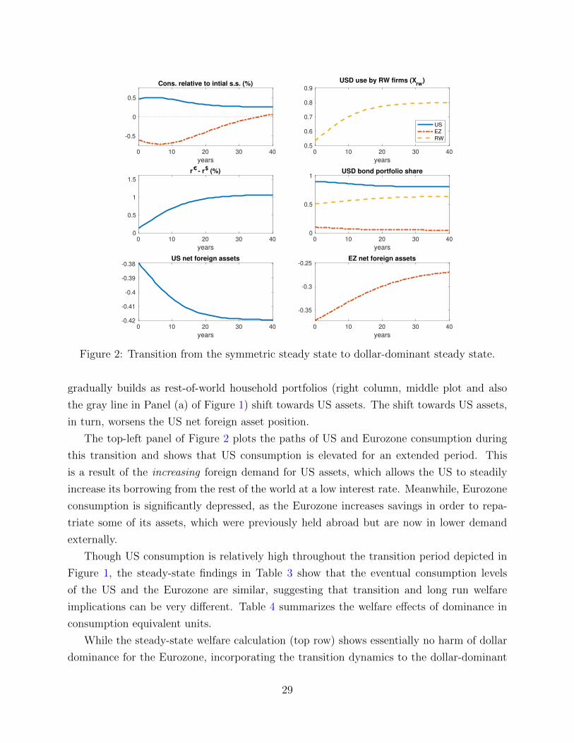
We next explore the transition paths that underly Figure 1 in more detail. As an example,

Figure 2 plots the transition of several endogenous variables, when the economy starts at the

(unstable) symmetric steady state and converges to the dollar-dominant steady state. The

top right panel shows the evolution of the equilibrium mix of collateral used (Xrw), which

starts close to equally balanced and then gradually converges to dominant dollar usage over

the subsequent 15 to 20 years. Along this transition path, the exorbitant privilege of the US

18We have also confirmed via linearization that the dominant equilibria are locally stable but the sym-metric steady state is not.

28

0 10 20 30 40

years

-0.5

0

0.5

Cons. relative to intial s.s. (%)

0 10 20 30 40

years

0.5

0.6

0.7

0.8

0.9

USD use by RW firms (Xrw

)

US

EZ

RW

0 10 20 30 40

years

0

0.5

1

1.5

r - r$ (%)

0 10 20 30 40

years

0

0.5

1USD bond portfolio share

0 10 20 30 40

years

-0.42

-0.41

-0.4

-0.39

-0.38US net foreign assets

0 10 20 30 40

years

-0.35

-0.3

-0.25EZ net foreign assets

Figure 2: Transition from the symmetric steady state to dollar-dominant steady state.

gradually builds as rest-of-world household portfolios (right column, middle plot and also

the gray line in Panel (a) of Figure 1) shift towards US assets. The shift towards US assets,

in turn, worsens the US net foreign asset position.

The top-left panel of Figure 2 plots the paths of US and Eurozone consumption during

this transition and shows that US consumption is elevated for an extended period. This

is a result of the increasing foreign demand for US assets, which allows the US to steadily

increase its borrowing from the rest of the world at a low interest rate. Meanwhile, Eurozone

consumption is significantly depressed, as the Eurozone increases savings in order to repa-

triate some of its assets, which were previously held abroad but are now in lower demand

externally.

Though US consumption is relatively high throughout the transition period depicted in

Figure 1, the steady-state findings in Table 3 show that the eventual consumption levels

of the US and the Eurozone are similar, suggesting that transition and long run welfare

implications can be very different. Table 4 summarizes the welfare effects of dominance in

consumption equivalent units.

While the steady-state welfare calculation (top row) shows essentially no harm of dollar

dominance for the Eurozone, incorporating the transition dynamics to the dollar-dominant

29

US EZ RW

steady-state only 0.25% 0.22% -0.12%

incl. transition 0.37% -0.37% -0.00%

Table 4: Welfare gain/loss at dollar-dominant steady state, as percentage of symmetricsteady state consumption.

steady state reverses this conclusion. Taking into account the transition period, in which

the US is able to maintain consumption significantly above its eventual steady-state level

for an extended period of time, the US permanent consumption equivalent is 0.75% higher

than that of the Eurozone. This is an order of magnitude larger than the 0.03% welfare

gain implied by steady-state consumption difference alone. Thus, accounting for both out

of steady state dynamics and general equilibrium portfolio and asset positions, is crucial for

properly assessing the welfare implications of issuing the dominant currency.

3.4 The emergence of dollar dominance

The model rationalizes the historical experience of prolonged dominant-asset regimes –

e.g. the British pound was dominant before the 1940s, and the US dollar since – because

only dominant-asset steady states are dynamically stable. But why is the dollar, specifically,

playing the dominant role currently? Our model suggests that both an initial advantage in

the US’s ability to supply safe assets and path dependence play important roles.

Regarding the dollar’s initial advantage, our model suggests two features were particularly

important. First, after WWII the US had a unique ability to credibly supply large quantities

of safe assets. Second, under the Bretton Woods agreement, the US was the only country

with virtually no capital controls, which facilitated international access to its (abundant)

supply of safe assets.19 In such an asymmetric world, our model implies that there in fact

exists only one steady state, with coordination on the single abundant asset the unique

outcome globally, which explains how the dollar established its initial post-war dominance.

Since the dollar gained dominance in world markets, however, the US has become less

unique both in terms of its ability to supply large quantities of a safe asset on a global

scale, and in terms of its economic size and central role in world trade. Because historical

19See Ghosh et al. (2020) for a detailed description of the evidence on capital controls. They also note thatthe US Treasury secretary at the time was well aware of the benefit of an open US capital account, havingstated in his 1948 testimony to Congress that controlling capital inflows would require exchange controlsthat “would do maximum violence to our position as a world financial center.”

30

experience suggests (occasional) transitions are possible, we next explore how empirically

relevant changes to the global economy might affect the dollar’s dominant position.

Introduction of the Euro

Many academics and policy makers once speculated that the formation of the Eurozone

might precipitate a shift in the equilibrium (e.g. Chinn and Frankel, 2007). In our model, the

emergence of a Eurozone block similar to the US creates a second stable steady state, but

path dependence prevents the economy from transiting to it absent some other precipitating

shock. To illustrate this point, we simulate two alternative, counter-factual scenarios of the

euro introduction. In both cases, we take the starting point (i.e. the world pre-1999) as one

in which the supply of the alternative asset is 60% of the size of the US safe asset supply,

i.e. Be = 0.6B$, consistent with the supply of German bonds at the time. We then model

the formation of the Eurozone as an increase in the supply of the alternative safe asset over

time, reflecting the increased fiscal capacity of the Eurozone.20

Before exploring dynamics, we first look at the model’s steady-state implications before

the Eurozone is introduced. When the supply of the alternative asset is only 60% of that

of the US asset, we find the model has a unique, dollar-dominant steady state: The initial

asymmetry in the supply of the two assets is strong enough to guarantee world coordination

on the dollar. Initializing the economy at this steady state, we then consider the resulting

transition path(s) as the supply of Eurozone assets grows with the introduction of the euro.

In the first scenario, plotted in Figure 3 with a blue line, we assume that the total supply

of Eurozone safe assets converges to the same level as that of the US asset over a 10 year

period (i.e. to our benchmark calibration). The results of this exercises are displayed by

the blue line. We find that there is a unique transition path out of the dollar-dominant,

pre-Eurozone steady state, a path which converges to the new dollar-dominant steady state.

Along the transition path, dollar use, the interest rate differential, and the US net foreign

asset position are essentially unchanged, consistent with the continued dominance of the

dollar in the data. Thus, our model agrees that path dependence is too strong for the

introduction of the euro, by itself, to change the currency regime. The euro introduction

creates a new, euro-based steady state, but without further shocks, the world would not

converge to it.

In the second scenario, we consider the counter-factual possibility that the Eurozone

20We model a gradual transition because interest rates on euro-area sovereigns took several years toconverge to those of the German Bund, suggesting that markets only gradually accepted euro bonds as ahomogeneous safe asset.

31

1996 2007 2017 2027 2037

years

0.6

0.8

1

1.2

1.4EZ safe assets/US safe assets

EUR introduction

EUR continued growth

1996 2007 2017 2027 2037

years

0

0.5

1

USD use by RW firms (Xrw

)

1996 2007 2017 2027 2037

years

-2

-1

0

1

2r - r$ (%)

1996 2007 2017 2027 2037

years

0

0.2

0.4

0.6

0.8RW USD bond portfolio share

1996 2007 2017 2027 2037

years

-0.5

-0.4

-0.3

-0.2

-0.1US net foreign assets

1996 2007 2017 2027 2037

years

-2

-1

0US cons. relative to intial s.s. (%)

Figure 3: Introduction of euro

eventually grows significantly larger than the US, to the point that the euro-dominant steady

state becomes unique. Making the euro-dominant steady state unique requires the supply

of Eurozone assets to exceed the supply of US assets by 30%: i.e. Be

B$ > 1.3.

We plot this scenario with a red line in Figure 3. Along the path to the new, uniquely

stable euro-dominant steady state, the US net foreign asset position shrinks towards zero,

and the US’s exorbitant privilege benefits disappears as the US safe assets largely leave inter-

national markets and return to US portfolios. The welfare impact is significant: the welfare

swing between the US and the Eurozone is equivalent to 1.4% of permanent consumption.

The figure also highlights an insight that we can only derive thanks to the model’s

dynamic nature. Namely, there are significant anticipation effects, as much of the shift in

portfolios and international currency usage occurs before the supply of Eurozone assets has

actually converged to its new, high steady state. This means that a switch away from the

dollar-dominant regime could have occurred upon the creation of the Eurozone, if investors

around the world were convinced that additional countries such as the UK and Sweden

would eventually join, even if this consolidation never actually ends-up happening. Just the

expectation of further expansion, if held long enough for rest-of-world portfolios to rebalance

towards Eurozone assets, could have precipitated a change in currency regime.

32

Overall, these counterfactuals show that merely introducing a fundamentally equivalent

asset is not enough to shift the currency regime; to become dominant, the alternative asset

needs to offer a substantially bigger base than the dollar, now or in the future. Yet, the 30%

threshold implied by the model is not so extreme, and it could realistically be surpassed by

either the Eurozone or China in the future.

Growth of the Rest-of-world

The US share of world output has shrunk by roughly 15 percentage points since 1960,

with a corresponding rise in the output share of developing (non-G7) countries. A natural

question is whether this fall in the relative size of the US imperiled the dominance of the US

dollar or if, by contrast, it actually increased the benefits of issuing the dominant currency

since the dollar asset intermediates a now larger quantity of rest-of-world trade.

To explore this question, we consider a counter-factual experiment in which the US

starts as the largest economy and gradually shrinks (from µus = 0.35 to 0.20, our benchmark

calibration), while the rest-of-world reciprocally grows (from µrw = 0.45 to 0.60). To isolate

the effects of size, we hold constant the aggregate supply of US and euro bonds, B.21

A first insight is that at the starting point where the US is substantially bigger than

the Eurozone again there exists only one steady state, at which the dollar is dominant.

In this case, the use of dollars in the rest of the world is anchored by the relatively high

probability that rest-of-world firms will trade with dollar-intensive US firms. The fall in the

size of the US opens the possibility of a change in the dominant currency, as our benchmark

calibration features two stable steady states. In this sense, our model implies that the dollar’s

dominance has become more fragile over the last sixty years, both because of the introduction

of alternative assets and because of the US’s reduced share of the global economy.

To understand whether the changing relative economic size of the US had a material

impact on the US’s dominance in practice, Figure 4 plots the evolution of several key variables

as the economy follows the (unique) transition path, which leads to the dollar-dominant

steady state of our symmetric baseline model. The top-right panel of the figure shows that,

as the US shrinks, the intensity of the rest-of-world dollar usage (Xrw) falls somewhat but

the dollar clearly remains dominant. The intensity of dollar use falls because rest-of-world

trading firms now face a substantially smaller chance of encountering US firms, who primarily

21One subtlety in performing this exercise is that changing country size also changes the relative supplyof each country-specific good, which impacts relative prices. To control for this, we adjust the Cobb-Douglasshares in preferences so that (in a frictionless economy) the size changes have no effect on relative prices.Since this is a change in preferences, we refrain from making welfare comparisons.

33

1960 1975 1990 2005 2020

years

0.2

0.3

0.4

0.5

0.6Size

us

rw

1960 1975 1990 2005 2020

years

0.8

0.85

0.9

0.95

USD use by RW firms (Xrw

)

1960 1975 1990 2005 2020

years

0.5

1

1.5

r - r$ (%)

1960 1975 1990 2005 20200.7

0.8

0.9

1

1.1

RW USD bond holdings

Figure 4: Growth of rest-of-world

use dollars in their trading activity. This reduces their incentive to use dollars, a reduction

that is reinforced by strategic incentives in general equilibrium.

Even though average use of dollars among rest-of-world firms falls, the mass of rest-of-

world firms that use dollars actually grows due to the increase in the economic size of the

rest-of-world countries. This, in turn, increases the total external demand for US assets (due

to the increased volume of dollar-denominated trade), as can be seen from the bottom right

panel of Figure 4 (Brw). Overall, the US’s shrinking size gives rise to offsetting effects on

US dominance, which on net leave the US in a similar position in 2020 as it was in 1960 —

the clear hegemon, with a somewhat lower exorbitant privilege in terms of the interest rate

spread re − r$ (bottom left panel of the Figure, mainly due to fall in Xrw), but enjoying a

higher overall external demand for its assets.

These implications track the historical experience. The US has indeed remained dominant

through the last sixty years, although that dominance is somewhat less pronounced given the

small but rising share of “other” currencies used internationally as compared to sixty years

ago. Still, our model implies that the US is managing to extract a similarly large effective

seignorage, thanks to the increased volume of international trade.

Comparison to Gopinath and Stein (2020)

The predictions explored in the above experiments contrast with other models. For

example, according to the model of Gopinath and Stein (2020), increasing the supply of an

asset (our first experiment) should decrease the likelihood it become dominant whereas our

34

model implies the reverse.22 Similarly, in their model, increasing the quantity of world trade

while keeping asset supplies constant should have significantly boosted dollar dominance.

While these alternative mechanisms need not be mutually exclusive, we think historical

experience favors the sort of relationship implied by our model. First, a strong empirical

pattern is that the hegemon country carries a substantial negative net foreign asset position,

as exemplified by the persistent US imbalance. This observation is explained endogenously

by our model – an asset that is dominant must be widely held abroad – but seems in tension

with their model in which the special asset is the scarce one.

Second, historical accounts of the emergence of the dollar tend to emphasize the impor-

tance of dollar “availability” rather than “scarcity.” For example, Eichengreen and Flandreau

(2012) documents the crucial role played by the Federal Reserve Act of 1913, which signif-

icantly increased the availability of offshore dollar trade financing, in jump-starting the US

dollar’s international role. More recently, Bahaj and Reis (2020) document a similar effect

in terms of the growing importance of the Chinese renminbi and the increased number of

swap agreements the Chinese Central Bank has signed with rest-of-world counterparts.

As a final piece of suggestive evidence, our online Appendix C documents two stylized

patterns in cross-sectional data that support the hypothesis that asset availability favors an

asset’s dominant status. In that appendix, we relate a country’s holdings of US Treasuries

with the use of dollars in invoicing and the issuance of dollar-denominated bank liabilities.

In the first case, we find that larger holdings of Treasuries in country i are associated

with higher dollar invoicing. In the second case, we find that larger holdings of Treasuries

in country i are associated with greater issuance of dollar bank liabilities in that country.23

Both results seem to contrast with the mechanism in Gopinath and Stein (2020), which relies

on the offshore scarcity of the dominant asset, but are consistent with our model which relies

instead on wide-spread holdings of an asset to drive dominance. Since these are correlations,

not causal relationships, we view the results as only suggestive evidence.

Finally, we note there is no tension between our theoretical findings and the empirical ev-

idence of e.g. Krishnanurthy and Vissing-Jorgensen (2011) that asset supply and convenience

yields are negatively correlated. In our model, the positive association between supply and

liquidity premia appears only when comparing steady states. By contrast, local increases in

an asset’s supply will still imply a fall in its liquidity premium, just as in the data.

22For example, they highlight this implication in their discussion of proposals for a “Eurobond” in Section5.3, noting their model implies such a development should only harm the Euro’s international status.

23We use invoicing because the data on currency composition of trade finance in the cross-section issparser. However, studies by BIS (2014) and Friberg and Wilander (2008) suggest that in the data thecurrency of invoicing is very highly correlated with the trade finance currency.

35

0.2 0.3 0.4 0.5 0.6 0.7 0.8

0.2

0.3

0.4

0.5

0.6

0.7

0.8Euro

Indet.

(a) Attraction regions, moderate trade war

0.2 0.3 0.4 0.5 0.6 0.7 0.8

0.2

0.3

0.4

0.5

0.6

0.7

0.8

(b) Attraction regions, acute trade war

Notes: Left panel depicts regions of attraction assuming long-lived tariffs of 15%; right panel depicts attraction regions, assuming

long-lived tariffs of 30%. The right panel shows that only the Euro can be dominant in the long run in the acute trade war scenario.

Figure 5: Attraction regions under trade war scenarios.

3.5 Trade Policy and Barriers

Recent trade conflicts between the US and other countries have raised the possibility that

trade barriers might affect the currency regime. To shed some light on this, we consider two

“trade war” scenarios in which the US introduces a proportional tariff γ on all imports and

the Eurozone and rest-of-world countries respond by levying the same tariffs on US imports.

Tariffs are implemented as taxes paid by consumers, so while US importers receive the

price of P jus,t for each imported type j good, US consumers pay the effective price

P jus,t = (1 + γ)P j

us,t.

Similarly, Eurozone and rest-of-world consumers pay import taxes on US imports, and hence

face the prices P usjt = (1 + γ)P us

jt . In all countries, tariff revenues are reimbursed lump-sum

to households. Even though they are refunded, the tariffs lead to expenditure switching on

the consumer side, and thus also shift the equilibrium patterns of trade flows. We consider

two scenarios, a “moderate” trade war where γ = 0.15 and an “acute” one where γ = 0.30.

36

US EZ RW

Dollar remains dominant -1.34% 0.07% 0.09%

Euro becomes dominant -2.13% 0.79% 0.10%

Table 5: Gain/loss as percentage of dollar-dominant steady state consumption.

Moderate Trade War

Figure 5, Panel (a) depicts the consequences of a permanent trade war, with tariffs set

to γ = 0.15. The tariffs change the position of the steady states and also their respective

attraction regions (old steady states are marked with ×; the new steady states with a dot).

As the figure shows, the region of unique attraction to the dollar-dominant steady state is

eliminated, and both the old and new dollar-dominant steady states lie within the region of

equilibrium indeterminacy. Moreover, the region of unique attraction to the euro-dominant

steady state is significantly increased. Hence, even a moderate trade war could potentially

endanger the position of the dollar, as it makes the dollar-dominant regime unstable.

The trade war weakens dollar dominance for two reasons. First, it diverts rest-of-world

trade away from the US and towards the Eurozone. Since Eurozone firms are far more likely

to use Eurozone assets in their trade, rest-of-world firms become more likely to encounter

euro-funded trading partners and, hence, to prefer euros. Second, the overall world trade

level falls, decreasing trade quantities relative to total asset supply. As trade financing

become less scarce, the equilibrium anchoring effects of the financial friction become weaker,

increasing the indeterminacy region.

The first row of Table 5 reports the welfare implications of the moderate trade war,

assuming the dollar remains dominant. The US is disproportionately hurt by the trade war

for two reasons. First, there is the standard effect from the fact that the distortions created

by the tariffs hit all of its exports, while the Eurozone and the rest-of-world face tariffs only

on their direct trade with the US. Second, as world trade levels fall, the US’s seignorage

revenue decreases as both fewer firms require liquidity and a smaller portion choose dollars.

Since the starting position of the economy (i.e. the dollar-dominant steady state before

the tariffs) is now inside the indeterminate region, however, this is not the only possible

outcome. In the second row of Table 5, we report the welfare implications of the same trade

war scenario, but assuming the alternative long-run outcome that is now possible – that the

dollar looses dominance and the economy transitions to the euro steady state.

In this second case, the US is significantly worse off and Eurozone welfare is substantially

37

improved. On the one hand, at the new steady state the US loses all of its seignorage, as the

world currency use and the resulting exorbitant privilege shift to the Eurozone. On the other

hand, the transition to this new steady state itself, depicted by the long gray line in Panel

(a) of Figure 5, is particularly painful because during the transition the US runs significant

trade surpluses as external demand for dollar assets dries up.

The welfare difference between the US and Eurozone when the euro becomes dominant is

2.9% of permanent consumption. Comparing to the first line of the table, where the US-EZ

welfare differential is 1.4%, we conclude that the loss of currency dominance is worth 1.5%

of permanent consumption. Moreover, we also find that the transition dynamics generate

two-thirds of this effect, hence a steady-state-only model would understate the cost of losing

special status by a factor of three.

Acute Trade War

Figure 5, Panel (b) depicts the implications of a permanent 30% tariff between the US

and Eurozone/rest-of-world, a scenario we call an “acute” trade war. In this case, the effects

of the trade barriers are strong enough to eliminate the symmetric and the dollar-dominant

steady states, thereby guaranteeing a transition to the now-unique euro steady state.

This is a strong implication, but a permanent 30% tariff on all imports is (we hope)

implausible. Hence, we also consider the effects of a temporary trade war of the same

magnitude. Figure 6 depicts the welfare cost for different possible durations, ranging from

one to 40 years. The figure shows that for trade wars lasting under 10 years, the economy

cannot transition to the euro steady state absent other shocks. Within this range, longer

trade wars are worse but not discretely so, highlighting the general stability of the model:

Even 10 years of a very acute trade war is not enough to shift the currency regime.

For trade wars lasting more than 10 years, however, the economy enters a region of

indeterminacy, and a transition to the euro-dominant steady state becomes possible. If a

transition occurs, the US is discretely worse off, and suffers an additional loss of roughly 1%

of permanent consumption. If the trade war lasts longer than 28 years, the unique outcome

is a transition to the euro-dominant steady state, despite the fact that tariffs return to zero

in the long-run. Thus, certain temporary shocks, could have permanent effects.

38

1 10 20 30 40

years

-4

-3

-2

-1

0

1

co

ns.

eq

uiv

ale

nt

US

Dollar in long run

Euro in long run

1 10 20 30 40

years

-4

-3

-2

-1

0

1

co

ns.

eq

uiv

ale

nt

EZ

1 10 20 30 40

years

-4

-3

-2

-1

0

1

co

ns.

eq

uiv

ale

nt

RW

Figure 6: Welfare costs of an acute trade war as a function of duration.

4 Conclusions

This paper presents a new theory describing the emergence of dominant international as-

sets. Our model is quantitatively realistic and tractable enough to use for standard macroe-

conomic analysis. Throughout, we have abstracted from risk: both the potential for short

run shocks that perturb the economy around a given steady state and possible longer-run

stochastic transitions between currency regimes. Both of these extensions are straightfor-

ward: Business-cycle analysis can be conducted using policy functions approximated locally

around a given steady state, or via global solution techniques. Such extensions could help

the model address the observation of Gourinchas et al. (2017) that an “exorbitant duty”

coincides with the privilege of being the dominant currency. We leave exploration of this

issue to future work.

5 Data Availability

The data and code underlying the results in this article are available in Zenodo at

https://doi.org/10.5281/zenodo.5544238.

References

Ahn, J. (2014). Understanding Trade Finance: Theory and Evidence from Transaction-levelData. Unpublished. International Monetary Fund .

39

Amiti, M., O. Itskhoki, and J. Konings (2018). Dominant Currencies How Firms ChooseCurrency Invoicing and Why It Matters. National Bank of Belgium, Working paper No.353.

Amiti, M. and D. E. Weinstein (2011). Exports and Financial Shocks. The Quarterly Journalof Economics 126 (4), 1841–1877.

Antras, P. and A. Costinot (2011). Intermediated trade. The Quarterly Journal of Eco-nomics 126 (3), 1319–1374.

Antras, P. and C. F. Foley (2015). Poultry in Motion: A Study of International TradeFinance Practices. Journal of Political Economy 123 (4), 853–901.

Auboin, M. (2016). Improving the availability of trade finance in developing countries: Anassessment of remaining gaps. CESifo Working Paper Series No. 5784.

Bahaj, S. and R. Reis (2020). Jumpstarting an international currency. CEPR DiscussionPaper No. DP14793.

Bianchi, J., J. C. Hatchondo, and L. Martinez (2018). International reserves and rolloverrisk. American Economic Review 108 (9), 2629–70.

BIS (2014). Trade Finance: Developments and Issues. CGFS Papers No. 50.

Bocola, L. and G. Lorenzoni (2020). Financial crises, dollarization, and lending of last resortin open economies. American Economic Review 110 (8), 2524–57.

Bonetti, G. (2018). The FX Dilemma: An Introduction to Hedging Currency Risk in BondPortfolios. Technical report, PIMCO.

Brunnermeier, M. K. and L. Huang (2018). A global safe asset for and from emerging marketeconomies. Working Paper 25373, National Bureau of Economic Research.

Bruno, V. and H. S. Shin (2019). Dollar exchange rate as a credit supply factor–evidencefrom firm-level exports. BIS Working Paper No. 819.

Caballero, R. J., E. Farhi, and P.-O. Gourinchas (2008). An Equilibrium Model of “GlobalImbalances” and Low Interest Rates. American Economic Review 98 (1), 358–93.

Chahrour, R. and R. Valchev (2017). International Medium of Exchange: Privilege andDuty. Boston College Working Paper No. 934.

Chinn, M. and J. A. Frankel (2007, May). Will the Euro Eventually Surpass the Dollar AsLeading International Reserve Currency?, pp. 283–338. University of Chicago Press.

Cosar, A. K., P. L. Grieco, S. Li, and F. Tintelnot (2018). What Drives Home MarketAdvantage? Journal of International Economics 110, 135–150.

40

den Haan, W. J., G. Ramey, and J. Watson (2000). Job Destruction and Propagation ofShocks. American Economic Review 90 (3), 482–498.

Devereux, M. B. and S. Shi (2013). Vehicle Currency. International Economic Review 54 (1),97–133.

Di Capria, A., S. Beck, Y. Yao, and F. Khan (2016). 2016 Trade Finance Gaps, Growth,and Jobs Survey. Asian Development Bank.

Doepke, M. and M. Schneider (2017). Money As a Unit of Account. Econometrica 85 (5),1537–1574.

Eaton, J., D. Jinkins, J. Tybout, and D. Xu (2016). Two-sided Search in InternationalMarkets. In 2016 Annual Meeting of the Society for Economic Dynamics.

Eichengreen, B. and M. Flandreau (2012). The Federal Reserve, the Bank of England, and therise of the dollar as an international currency, 1914–1939. Open Economies Review 23 (1),57–87.

Engel, C. (2006). Equivalence results for optimal pass-through, optimal indexing to exchangerates, and optimal choice of currency for export pricing. Journal of the European EconomicAssociation 4 (6), 1249–1260.

Eren, E. and S. Malamud (2021). Dominant currency debt. Journal of Financial Economics .

Farhi, E. and M. Maggiori (2017, 08). A Model of the International Monetary System. TheQuarterly Journal of Economics 133 (1), 295–355.

Friberg, R. and F. Wilander (2008). The currency denomination of exports – a questionnairestudy. Journal of International Economics 75 (1), 54–69.

Ghosh, A. R., J. I. Kim, and M. S. Qureshi (2020). What’s in a name? That which we callcapital controls. Economic Policy 35 (101), 147–208.

Goldberg, L. S. and C. Tille (2016). Micro, macro, and strategic forces in internationaltrade invoicing: Synthesis and novel patterns. Journal of International Economics 102,173–187.

Gopinath, G. (2016). The International Price System. In Jackson Hole Symposium Proceed-ings.

Gopinath, G., O. Itskhoki, and R. Rigobon (2010). Currency choice and exchange ratepass-through. American Economic Review 100 (1), 304–36.

Gopinath, G. and J. C. Stein (2020). Banking, Trade, and the Making of a DominantCurrency. The Quarterly Journal of Economics 136 (2), 783–830.

41

Gourinchas, P.-O. and H. Rey (2007a). From World Banker to World Venture Capitalist: USExternal Adjustment and the Exorbitant Privilege. In G7 Current Account Imbalances:Sustainability and Adjustment, pp. 11–66. University of Chicago Press.

Gourinchas, P.-O. and H. Rey (2007b). International Financial Adjustment. Journal ofPolitical Economy 115 (4), 665–703.

Gourinchas, P.-O., H. Rey, N. Govillot, et al. (2017). Exorbitant Privilege and ExorbitantDuty. Institute for Monetary and Economic Studies, Bank of Japan Discussion Paper No2010-E-20.

Gourinchas, P.-O., H. Rey, and M. Sauzet (2019). The international monetary and financialsystem. Annual Review of Economics 11 (1), 859–893.

Hassan, T. (2013). Country size, currency unions, and international asset returns. TheJournal of Finance 68 (6), 2269–2308.

He, Z., A. Krishnamurthy, and K. Milbradt (2019). A Model of Safe Asset Determination.American Economic Review 109 (4), 1230–62.

Hoefele, A., T. Schmidt-Eisenlohr, and Z. Yu (2016). Payment choice in internationaltrade: Theory and evidence from cross-country firm-level data. Canadian Journal ofEconomics/Revue canadienne d’economique 49 (1), 296–319.

Ilzetzki, E., C. M. Reinhart, and K. S. Rogoff (2019). Exchange arrangements enter-ing the twenty-first century: Which anchor will hold? The Quarterly Journal of Eco-nomics 134 (2), 599–646.

Jiang, Z., A. Krishnamurthy, and H. Lustig (2020). Dollar safety and the global financialcycle. Working Paper 27682, National Bureau of Economic Research.

Kannan, P. (2009). On the Welfare Benefits of an International Currency. European Eco-nomic Review 53 (5), 588 – 606.

Krishnanurthy, A. and A. Vissing-Jorgensen (2011). The Effects of Quantitative Easing OnInterest Rates: Channels and Implications For Policy. Brookings Papers on EconomicActivity , pp. 215–287.

Liu, T., D. Lu, and W. T. Woo (2019). Trade, finance and international currency. Journalof Economic Behavior & Organization 164, 374 – 413.

Maggiori, M. (2017). Financial Intermediation, International Risk Sharing, and ReserveCurrencies. American Economic Review 107 (10), 3038–71.

Mas-Colell, A., M. D. Whinston, J. R. Green, et al. (1995). Microeconomic Theory, Volume 1.Oxford University Press New York.

42

Matsuyama, K., N. Kiyotaki, and A. Matsui (1993, 04). Toward a Theory of InternationalCurrency. The Review of Economic Studies 60 (2), 283–307.

Mendoza, E. G., V. Quadrini, and J.-V. Rios-Rull (2009). Financial integration, financialdevelopment, and global imbalances. Journal of Political Economy 117 (3), 371–416.

Mukhin, D. (2018). An equilibrium model of the International Price System. Working Paper.

Niepmann, F. and T. Schmidt-Eisenlohr (2017). International Trade, Risk and the Role ofBanks. Journal of International Economics 107, 111–126.

Rey, H. (2001). International Trade and Currency Exchange. The Review of EconomicStudies 68 (2), 443–464.

Richmond, R. J. (2019). Trade network centrality and currency risk premia. The Journal ofFinance 74 (3), 1315–1361.

Schmidt-Eisenlohr, T. (2013). Towards a theory of trade finance. Journal of InternationalEconomics 91 (1), 96–112.

Vayanos, D. and P.-O. Weill (2008). A search-based theory of the on-the-run phenomenon.The Journal of Finance 63 (3), 1361–1398.

Weill, P.-O. (2008). Liquidity premia in dynamic bargaining markets. Journal of EconomicTheory 140 (1), 66–96.

Wright, R. and A. Trejos (2001). International Currency. Advances in Macroeconomics 1 (1).

Zhang, C. (2014). An Information-based Theory of International Currency. Journal ofInternational Economics 93 (2), 286 – 301.

Zhou, R. (1997). Currency Exchange in a Random Search Model. The Review of EconomicStudies 64 (2), 289–310.

Appendix

A Proofs

Proof of Lemma 1. First, we prove uniqueness. We aim to show that, under the condition

in the Lemma, the quasi-equilibrium correspondence X(B$rw, B

erw) is a scalar for all possible

asset holdings. Since the total supply of each asset is B, then market clearing (B = µrwBcrw+

µusBcus + µezB

cez) puts an upper bound on the feasible rest-of-world asset holdings:

B$rw <

B

µrw, Berw <

B

µrw

43

If either B$rw = 0 or Berw = 0, it is trivially true that the quasi-equilibrium is unique. For

example, if Berw = 0 then

V $(Xrw) =B$rw

B$rw +Xrw

(π − r − κ(1−Xrwµrw − µus)) > 0

since κ < π − r. Thus, the only quasi-equilibrium in funding is Xrw = 1. Similarly, ifB$rw = 0, the only quasi-equilibrium is Xrw = 0.

Next, we show that for any pair of bond holdings {B$rw, B

erw}, such that B$ ∈ (0, B

µrw)

and Be ∈ (0, Bµrw

), the net payoff of using dollars crosses zero exactly once, thus the quasi-

equilibrium is unique. Using µus = µeu = 1−µrw2

, and evaluating equation (4) at Xrw = 1:

V $(1) = − π − rB$rw + 1

+ κµrw(B$

rw + 12) + 1

2

B$rw + 1

This is strictly negative (and thus Xrw = 1 is not a quasi-equilibrium) if and only if

κ <π − r

µrw(B$rw + 1

2) + 1

2

.

A similar argument implies that V $(0) > 0 if and only if

κ <π − r

µrw(Berw + 12) + 1

2

.

But since B$rw <

Bµrw

,

π − rµrw(B$

rw + 12) + 1

2

>π − r

B + µrw2

+ 12

= κsunspot

Thus, when κ < κsunspot, Xrw = 1 is not a quasi-equilibrium for any feasible allocationof asset holdings when B$ > 0 and Be > 0. Similar argument, shows that Xrw = 0 is nota quasi-equilibrium either in this case. Hence, all existing quasi-equilibria must be interiorand thus solve V $(Xrw) = 0.

Evaluating equation (4) gives:

V $(Xrw) =B$rw

B$rw +Xrw

[π − r − κ(1−Xrwµrw − µus)]−Berw

Berw + (1−Xrw)[π − r − κ(Xrwµrw + µez)] .

Setting the above expression equal to zero and multiplying by 1κ(B$

rw+Xrw)(Berw+(1−Xrw))results in a quadratic equation in Xrw. Simplifying further, and dividing through by κ, allowsus to express the resulting quadratic polynomial as P (Xrw):

P (Xrw) = (Berw −B$rw)µrwX

2rw

44

+

(B$rw

(1

2+

3

2µrw − 2

π − rκ

)+Berw

(1

2− µrw

2+ 2B$

rwµrw −π − rκ

))Xrw

+B$rw

(π − rκ−(

1

2+ µrw(Berw + 1)

))Since the quadratic polynomial P (Xrw) has different signs at P (0) and P (1), it can onlyhave a single crossing in the range X ∈ (0, 1) and thus there is a unique quasi-equilibrium.

Let X∗ ∈ (0, 1) be the unique quasi-equilibrium value that satisfies P (X∗) = 0 for a given

level of bond holdings {B$rw, B

erw}. To see that X∗ > B$

rw

B$rw+Berw

whenever B$rw > Berw, notice

that if B$rw > Berw

P (Xrw =B$rw

B$rw +Berw

) =B$rwB

erwµrw

(B$rw(1 +B$

rw)−Berw(1 +Berw))

(Berw +B$rw)2

> 0.

Hence since P (1) < 0, the zero of the quadratic polynomial P (X) must be at a value

X∗ > B$rw

B$rw+Berw

.

To prove that κ < π−rB$+µrw

2+ 1

2

is a sufficient condition for uniqueness, let κ > π−rB+µrw

2+ 1

2

and note that if B$rw = B

µrwand Berw = B

µrw:

V $(1) = − π − rB$rw + 1

+ κµrw(B$

rw + 12) + 1

2

B$rw + 1

> 0

and

V $(0) =π − rB$rw + 1

− κµrw(B$

rw + 12) + 1

2

B$rw + 1

< 0

Thus, in this case both 1 and 0 are quasi-equilibria, and hence X( Bµrw

, Bµrw

) is set valued,

Hence, X(B$rw, B

erw) is not a scalar-valued function across the whole state space, and we

conclude the quasi-equilibrium is not always unique.�

Proof of Lemma 2. Throughout, let j ∈ [0, µrw] be an arbitrary index for a small openeconomy. Accounting explicitly for the inequality constraint in bonds, the steady-state Eulerequations (2) for dollars can be written

1

β=

1

Q$ −∆$j

+ λ$j =

1

Q$ −∆$us

+ λ$us =

1

Q$ −∆$eu

+ λ$eu, (18)

where the weakly positive λ’s are appropriately-scaled Lagrange multipliers and the comple-mentarity slackness conditions

λjB$j = λusB

$us = λeuB

$eu = 0 (19)

must hold for all countries.

45

We being by proving the following additional Lemma which would be helpful:

Lemma 3. B$j = 0 if and only if Xj = 0. Similarly, Bej = 0 if and only if Xj = 1.

We prove the statement for dollar bond holdings, the statement for euro holdings followsby a parallel argument.

If: If Xj = Xez = 0 the premia ∆$j = ∆$

eu = 0 by equation (6), while ∆$us > 0. Hence

equation (18) reduces to

1

Q$+ λ$

j =1

Q$+ λ$

ez =1

Q$ −∆$us

+ λ$us. (20)

But this equation shows that λj > λus and λez > λus. Since λus ≥ 0, we know that λj > 0and λez > 0 and, from complementary slackness, that B$

j = B$eu = 0.

Only If: To find a contradiction, suppose that Xj > 0 but B$j = 0. Since B$

j = 0, inequilibrium there must be some other country j′ (it could be the US or it could be anothersmall country) which holds positive amount of US bonds and pays premium ∆$

j′ < r. In thiscase, equation (18) implies

1

Q$ −∆$j′

=1

Q$ − r+ λ$

j . (21)

which cannot be true since λ$j ≥ 0. Hence, B$

j > 0. And the helper Lemma 3 is proved.

An implication of the proof above is that B$ez = Beus = 0. We can now use the equality

of the remaining premia along with market clearing conditions to compute the expressionsin the text. For example, ∆$

us = ∆$j implies that

Xj

B$j +Xj

=Xus

B$us +Xus

,

which simplifies to

B$us = B$

j

Xus

Xj

.

Using this expression and the fact that Bez = 0, B$us and B$

ez can be eliminated in the marketclearing condition for dollar bonds.

B =

∫µrw

B$us

Xus

Xidi+ µusB$us (22)

B =B$j

Xj

∫µrw

Xidi+ µusB$j

Xj

. (23)

Where in the second line we pick a specific country j and substitute in Xus = 1. Solvingexpression (23) for B$

j gives equation (8) in the Lemma 2. The same steps for euro bondsimply equation (9).

�

46

Proof of Proposition 1. To show that the dollar-dominant steady state exists, conjecturethat the rest-of-world traders all use dollars and thus Xrw = 1. Using Lemma 2, the optimalbond holdings of the rest-of-world households are then

B$rw =

B

B + µrw + µus

Berw = 0.

Plugging those expression into the relative payoff of seeking dollar vs euro funding for arest-of-world trader (V $), we have:

V $ =B

B + µrw + µus(π − r − κ(1− µrw − µus)) > 0.

Thus, using dollars is strictly preferred by any rest-of-world trader, and the dollar dominantsteady state where Xrw = 1 is indeed sustained. Conjecturing Xrw = 0, instead, andfollowing a similar argument shows that the euro-dominant steady state X = 0 also exists.

Lastly, we look for interior steady-state equilibria where Xrw ∈ (0, 1). In that, case theoptimal bond holdings for the rest-of-world households are given by:

B$rw = B

Xrw

µrwXrw + µus

Berw = B1−Xrw

µrw(1−Xrw) + µez

Substituting in those expressions for bond holdings in the value of seeking dollar collateralrelative to euro collateral for a rest-of-world trader, we have

V $(Xrw) =B

B + µrwXrw + µus[π − r − κ(1−Xrwµrw − µus)]−

B

B + µrw(1−Xrw) + µez[π − r − κ(Xrwµrw + µus)] . (24)

Any interior equilibrium must satisfy V (Xrw) = 0 – these are the points at whichthe traders are indifferent between seeking dollar and euro financing. To find the zerosof V $(Xrw), we set (24) equal to 0, and multiply through with (B + µrwXrw + µus)(B +µrw(1−Xrw) + µez). Then further dividing by B, gives us the condition

(B+µrw(1−Xrw)+µez) [π − r − κ(1−Xrwµrw − µus)]−(B+µrwXrw+µus) [π − r − κ(Xrwµrw + µus)] = 0

Using the fact that µus = µez and µus + µeu + µrw = 1, this equation simplifies to

µrw(κ(B + 1)− π − r)(2Xrw − 1) = 0.

47

This linear equation has the unique solution Xrw = 12

when κ 6= π−rB+1

, and admits any

Xrw ∈ [0, 1] as a solution in the knife edge case κ = π−rB+1

. Thus, for any κ ≥ 0 that is

different from π−rB+1

there are three steady states, Xrw ∈ {0, 12, 1}, and when κ = π−r

B+1there

is a continuum of steady states Xrw ∈ [0, 1]. The associated steady-state bond holdings arethen immediately implied by Lemma 2. �

Proof of Proposition 2. To prove local stability of a steady state, we need to show that thebest-response functions define a contraction in the neighborhood of that steady state. Definethe vector of best response functions of trading firms and households in country j, given theactions of all other firms, Xrw, and households in the rest of the world B$

rw and Berw:

ϕX(X,B$, Be) =B$(π − κ(Be + 1) + κ(µrwX + µus)(2B

e + 1))

(B$ +Be)π + κ((µrwX + µus)(B$ −Be)−B$)

ϕB$(X,B$, Be) = BX

µrwX + µus

ϕBe(X,B$, Be) = B

1−Xµrw(1−X) + µez

Stacking these in the vector Φ ≡ [ϕX , ϕB$ , ϕBe ], we want to show that Φ is a local contractionmap, which is the case whenever the eigenvalues of the Jacobian OΦ lie inside the unit circle.

The Jacobian has the form

OΦ =

∂ϕX∂X

∂ϕX∂B$

∂ϕX∂Be

∂ϕB$

∂X0 0

∂ϕBe

∂X0 0

hence its eigenvalues are given by the roots of the characteristic polynomial

λ

(λ2 − λ∂ϕX

∂X− ∂ϕX∂B$

∂ϕB$

∂X− ∂ϕX∂Be

∂ϕBe

∂X

)= 0.

Clearly, one solutions is λ = 0, but we need to check that the roots of the quadratic term inthe parenthesis are smaller than unity. We now check this condition for each steady state.

Case I: Symmetric Steady State

At the symmetric steady state we have that ∂ϕX∂B$ = −∂ϕX

∂Beand

∂ϕB$

∂X= −∂ϕ

Be

∂X. Hence, the

relevant condition for the eigenvalues reduces to

λ2 − λ∂ϕX∂X− 2

∂ϕX∂B$

∂ϕB$

∂X= 0

48

with roots

λ∗ =1

2

∂ϕX∂X±

√(∂ϕX∂X

)2

+ 8∂ϕX∂B$

∂ϕB$

∂X

.

At the symmetric steady state.

∂ϕX∂X

=(1 + 2B)κµrw

2π − κ> 0

since κ < π. Hence, the bigger root (in absolute value) is

λ∗ =1

2

∂ϕX∂X

+

√(∂ϕX∂X

)2

+ 8∂ϕX∂B$

∂ϕB$

∂X

.

Lastly, since we also have that

∂∂ϕ

B$

∂X

∂κ=∂ ∂ϕX∂B$

∂κ= 0,

the root is growing in κ. The threshold κ that ensures the root is within the unit circle solvesλ∗ = 1, which after some re-arranging results in:

1− ∂ϕX∂X− 2

∂ϕX∂B$

∂ϕB$

∂X= 0.

Solving for the threshold κ, we obtain

κ =π − rB + 1

Hence, in the neighborhood of the symmetric steady state, the roots of the characteristicpolynomial are inside the unit circle so long as κ < κ.

Case II: Dollar-dominant Steady State

At the dollar dominant steady state Xrw = 1 and

∂ϕX∂X

=∂ϕX∂B$

= 0.

Hence the roots λ are given by

λ2 =∂ϕBe

∂X

∂ϕX∂Be

where∂ϕBe

∂X

∂ϕX∂Be

=(1 + µrw)(π − r)− κ(1

2+ µrw(1 + 2B + µrw

2))

(1− µrw)(π − r − κ2(1− µrw))

.

If κ < (π−r)(1+µrw)12

+µrw(1+2B+µrw2

)then the above expression is positive. In that case, if it is also

49

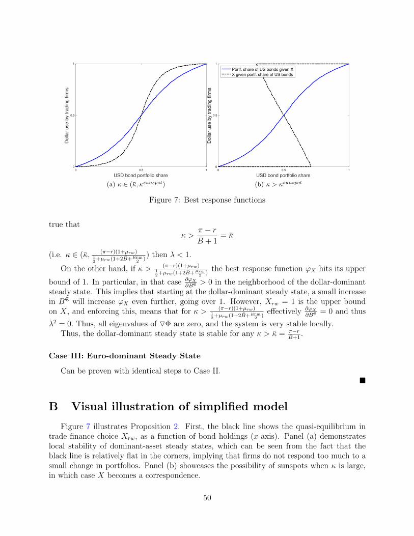
0 0.5 1

USD bond portfolio share

0

0.5

1D

olla

r use b

y tra

din

g firm

s

(a) κ ∈ (κ, κsunspot)

0 0.5 1

USD bond portfolio share

0

0.5

1

Dolla

r use b

y tra

din

g firm

s

Portf. share of US bonds given X

X given portf. share of US bonds

(b) κ > κsunspot

Figure 7: Best response functions

true that

κ >π − rB + 1

= κ

(i.e. κ ∈ (κ, (π−r)(1+µrw)12

+µrw(1+2B+µrw2

)) then λ < 1.

On the other hand, if κ > (π−r)(1+µrw)12

+µrw(1+2B+µrw2

)the best response function ϕX hits its upper

bound of 1. In particular, in that case ∂ϕX∂Be

> 0 in the neighborhood of the dollar-dominantsteady state. This implies that starting at the dollar-dominant steady state, a small increasein Be will increase ϕX even further, going over 1. However, Xrw = 1 is the upper boundon X, and enforcing this, means that for κ > (π−r)(1+µrw)

12

+µrw(1+2B+µrw2

)effectively ∂ϕX

∂Be= 0 and thus

λ2 = 0. Thus, all eigenvalues of OΦ are zero, and the system is very stable locally.Thus, the dollar-dominant steady state is stable for any κ > κ = π−r

B+1.

Case III: Euro-dominant Steady State

Can be proven with identical steps to Case II.�

B Visual illustration of simplified model

Figure 7 illustrates Proposition 2. First, the black line shows the quasi-equilibrium intrade finance choice Xrw, as a function of bond holdings (x-axis). Panel (a) demonstrateslocal stability of dominant-asset steady states, which can be seen from the fact that theblack line is relatively flat in the corners, implying that firms do not respond too much to asmall change in portfolios. Panel (b) showcases the possibility of sunspots when κ is large,in which case X becomes a correspondence.

50