TI 2003-060/2 Tinbergen Institute Discussion Paper

Trade Liberalization and Developing Countries under the Doha Round

J. Francois1

H. van Meijl2

F. van Tongeren2

1 Faculty of Economics, Erasmus University Rotterdam, Tinbergen Institute, and CEPR, 2 LEI, Wageningen University and Research Centre.

Tinbergen Institute The Tinbergen Institute is the institute for economic research of the Erasmus Universiteit Rotterdam, Universiteit van Amsterdam, and Vrije Universiteit Amsterdam. Tinbergen Institute Amsterdam Roetersstraat 31 1018 WB Amsterdam The Netherlands Tel.: +31(0)20 551 3500 Fax: +31(0)20 551 3555 Tinbergen Institute Rotterdam Burg. Oudlaan 50 3062 PA Rotterdam The Netherlands Tel.: +31(0)10 408 8900 Fax: +31(0)10 408 9031 Please send questions and/or remarks of non-scientific nature to driessen@tinbergen.nl. Most TI discussion papers can be downloaded at http://www.tinbergen.nl.

Trade Liberalization and Developing Countries Under the Doha Round †

J. Francois*, H. van Meijl**, F. van Tongeren**

August 2003

ABSTRACT: We explore the impact of multilateral liberalization, with emphasis on distributional effects across countries. We first develop a realistic "baseline" that takes into account events such as the entry of China into the WTO and the enlargement of the EU, allowing us to focus on those effects that are specifically attributable to further trade liberalization in the Doha Round. We then employ a global applied general equilibrium model, featuring capital accumulation and imperfect competition. Our Doha scenarios include agriculture, manufactures, and services liberalization, and trade facilitation. With agglomeration, OECD agricultural liberalization is not uniformly positive for developing countries. Keywords: WTO; Doha Round; trade liberalization; services trade, trade facilitation, CGE modeling JEL codes: F13, F4, F12

† We gratefully acknowledge support from the Netherlands Ministry of Economic Affairs, Directorate-General for Foreign Economic Relations, the World Bank, and the EU’s research and training networks (RTN) program. Particular thanks are due to Marko Bos, Arjan Lejour, and Gerrit Meester * Tinbergen Institute and CEPR ** LEI, Wageningen University and Research Centre Contact: Dr. J.F. Francois, Erasmus University Rotterdam, Burg Oudlaan 50-H8-18, 3000DR Rotterdam, Netherlands. ph: +31 10 408 1391, fax: +31 10 408 1946.

1

Trade Liberalization and Developing Countries Under the Doha Round

ABSTRACT: We explore the impact of multilateral liberalization, with emphasis on distributional effects across countries. We first develop a realistic "baseline" that takes into account events such as the entry of China into the WTO and the enlargement of the EU, allowing us to focus on those effects that are specifically attributable to further trade liberalization in the Doha Round. We then employ a global applied general equilibrium model, featuring capital accumulation and imperfect competition. Our Doha scenarios include agriculture, manufactures, and services liberalization, and trade facilitation. With agglomeration, OECD agricultural liberalization is not uniformly positive for developing countries. Keywords: WTO; Doha Round; trade liberalization; services trade, trade facilitation, CGE modeling JEL codes: F13, F4, F12

1. Introduction

After the failed attempts in Seattle in late 1999, the Ministerial Meeting of the World Trade

Organization (WTO) in Doha, in November 2001 launched the agenda for a new comprehensive

round of multilateral trade negotiations. At the behest of the EU, the ministerial declaration

emphasized that the Doha Round should provide a major opportunity for developing countries.

Consequently the agenda for new WTO round has been coined the ‘Doha Development

Agenda’. In this paper we explore the likely economic effects of the new WTO “Doha

Development Round” for major developed and developing regions. While the methodology

employed is comparable to that used in recent studies of these issues, we extend this literature by

including market structure and investment effects in the modeling exercise, and by stressing a

policy benchmark including China’s accession to the WTO, the Agenda 2000 reforms to the

CAP, enlargement of the EU. We cover the areas of agricultural liberalization, liberalization in

industrial tariffs, liberalization in services trade, and trade facilitation measures. Our services

scenarios build on gravity-equation based estimates of services barriers.

The core of our analysis is structured around a set of scenarios. These scenarios are based

on alternative liberalization approaches for agriculture, manufactured goods, and services trade.

They are meant to illustrate the implications of alternative approaches to market access

liberalization. They are stylized rather than exact representations. In part, this is because we are

working with an aggregate model (i.e. we do not model trade at the 6-digit HS level), and as such

detailed treatment of all product-specific proposals is simply impossible. In addition, the actual

2

market access modalities remain to be worked out. In agriculture, domestic support may or may not

be affected, developing countries may or may not have to liberalize, and certain politically sensitive

sectors may yet again escape from meaningful liberalization. Our scenarios are themselves

decomposed into different components, related to specific sets of countries and specific sectors and

instruments. This offers the advantage of allowing us (or the reader) to construct rough

representations of hybrid liberalization experiments later, since individual components can be taken

from different scenarios and combined.1

The paper is organized as follows: Section 2 develops the liberalization scenarios for the

subsequent quantitative analysis. Section 3 describes briefly the modeling framework used.

Section 4 discusses the results of our liberalization scenarios. It starts with a section on global

results, proceeding with the results for the EU.

2. The Policy Landscape and Scenarios

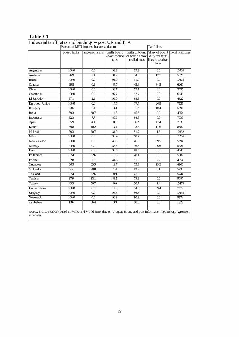
Tariff negotiations in the GATT/WTO have generally been based on tariff bindings, or

schedules of concessions tabled under GATT rules that define a maximum or ceiling rate for

trade restrictions. The coverage and level of these bindings is an important element of the initial

conditions for the negotiations. Table 2.1 provides information on the share of industrial-

product tariffs (on a trade-weighted basis) that remains either unbound or bound above applied

rates. While tariffs in the OECD (and Latin America) are generally bound, many Asian and

African economy tariffs remain unbound despite more than a four-fold increase in the coverage

of developing-country tariff bindings in the Uruguay Round (Abreu 1996). For almost all

developing countries, existing bindings are, on average, well above applied rates, reflecting a

combination of relatively high initial bindings, and the subsequent wave of reductions in applied

rates. (See Blackhurst et al 1996, Francois 2001).

In addition to general Uruguay Round commitments, there have also been efforts for

sector-based commitments to implement zero tariffs (called “zero-for-zero”). This is reflected in

the next-to-last column of Table 2-1. As a result of zero-for-zero efforts, OECD economies

have between roughly 10% and 30% of tariff lines bound at zero percent. Most developing

countries have opted out of this process. Zero-for-zero increased developed country duty-free

imports to 43% of total imports (Laird 1998). The process itself ground to a halt after the initial

1 Technically, decomposition of general equilibrium-related effects of policy scenarios exhibits path dependence, meaning that the decomposition can be sensitive to the ordering of the elements of the experiment set. The impact of a particular instrument is also sensitive to the other members of the set. We employ a linear decomposition method in this paper that addresses the path dependence problem (Harrison et al 2000). As such, individual experiment elements are roughly additive.

3

Information Technology Agreement (ITA). This seems to have been for two reasons: (i) the

sectors in which OECD economies could easily reach agreement had already been included, and

(ii) those sectors remaining involve North-South issues not susceptible to this approach. In

other words, the cherries have been picked, leaving us with the hard nuts.

[Table 2.1 about here]

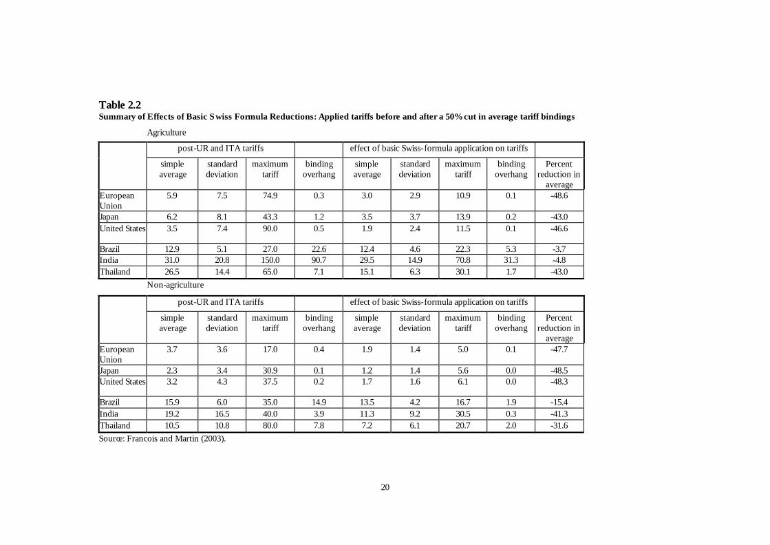
With the implementation of Uruguay Round commitments, average ad valorem tariffs in

the industrial countries generally are around 3 percent. This is reflected in the first columns of

Table 2.2.2 However, there are important exceptions. One of these is textiles and clothing,

where the average rate is roughly three times this overall average. This is reflected in the

standard deviation and maximum tariff columns. With full implementation of current

commitments, the estimated simple average industrial tariff in the United States is 3.2 percent,

with a standard deviation of 4.3, and a maximum tariff of 37.5 percent. The European Union

has a higher average, but less dispersion. (The EU has an average of 3.7 percent, a standard

deviation of 3.6 percent, and a maximum tariff of 17 percent.) For the developing countries in

Table 2.1, average industrial tariffs range from a low of 3 to 4 percent to a high of more than 20

percent. Table 2.2 presents detailed data for three developing countries: Brazil, India, and

Thailand. These countries span the spectrum of developing country bindings as reflected in

Table 2.1. Brazil’s tariffs are all bound, though the average rate for industrial products is 14.9

percentage points above the current applied rate. This gap is called a “binding overhang.” (See

Francois and Martin 2003.) India and Thailand’s tariffs are partially covered by bindings, again

with significant binding overhang. In general, for developing countries, binding overhang is large

enough that reductions in the range of 50% are necessary to force any reductions in average

applied rates for countries like Brazil. For many countries, even this will have little or no effect,

as tariffs are largely unbound. Of course, this limits severely the negotiating leverage of

developing countries in the WTO. This is also why the debate over using bound, applied, or

“historic” rates in the WTO as a starting point for negotiations is important.

[Table 2.2 about here]

2 For agriculture, Table 2.2 only covers notified ad valorem tariffs, and hence omits specific tariffs and quantity based measures that abound in agricultural trade.

4

As in the case of industrial tariffs, the stage for any future agriculture negotiations was

also set by the Uruguay Round outcome -- this time by the Uruguay Round Agreement on

Agriculture (URAA). One key difference from industrial products is that essentially all

agricultural tariffs are bound. However, in both industrial and developing countries, there is a

large degree of binding overhang resulting from “dirty tariffication” or the use of “ceiling

bindings” (Hathaway and Ingco 1996). The next round of agricultural negotiations was

scheduled in the URAA, while the negotiating parameters (tariffs, tariff-rate-quota levels, subsidy

commitments, etc.) must also be viewed in the context of the schedules of URAA commitments.

The system that has emerged is complex and similar to arrangements in the textile and clothing

sectors, featuring a mix of bilaterally allocated tariff-rate-quotas (with associated quota rents) and

tariffs. Viewed in conjunction with industrial protection, the basic pattern is that the industrial

countries protect agriculture and processed food, while protection in developing countries is

more balanced (though also higher overall) in its focus on food and non-food manufactured

goods.

The URAA had a stated goal of no backsliding and modest liberalization. However,

negotiating parties (generally the relevant agriculture ministries) gave considerable leeway to

themselves with regard to selection of the appropriate reference period from which to measure

export subsidy reductions. In addition, the move to a price-based system for protection has, in

many cases, been subsumed into an effective adoption of explicit quotas. The disciplines on

domestic subsidies have also been weakened by a relatively soft definition of the aggregate measure

of support (AMS) vis-à-vis individual subsidies and the scope for reallocation of expenditures within

the AMS. (See Tangermann 1998 for discussion.) Commitments not to erode current market

access were meant to limit the scope for increased protection through dirty tariffication. As the

name implies, dirty tariffication involved violations of the spirit, if not the letter, of the URAA text.

It involved setting tariff bindings at rates far above then current effective protection rates. The

practice of setting high bindings complicated the problem of measuring the impact of further

commitments to reduce bindings. Basically, in agriculture, we are in a world that allows scope for

great policy discretion and uncertainty as a result of the loose nature of the commitments made. In

addition, the setting of high bound rates made possible the conversion of NTBs into even more

restrictive import tariffs. This in turn made quantity disciplines necessary to avoid backsliding. As a

result, despite the stated goals of subsidy reductions and a shift toward price-based border measures,

one of the more striking features of the regime that has actually emerged from the URAA is the

prominent role that quantity measures have taken in the new architecture. Basically, the agricultural

trading system is complicated and still evolving. Policy measurement in this area has converged on

5

the use of price-based measurements that emphasize the tax/subsidy equivalent of policy. (As this

approach reflects available data, this is the approach we employ in this paper as well.)

For services, “market access” is a problematic concept. From the outset, service

negotiations have been "qualitative." They have not targeted numeric measures, but rather

commitments in the cross-border movement of consumers and providers and the establishment

of foreign providers. In fact, for academics, the GATS seems to confuse FDI and migration

with international trade. As a result, efforts to quantify market access in service sectors (a basic

requirement if we want to then quantify liberalization) have been problematic at best. The

standard approach (an example is Hoekman 1995) has been to produce inventory measures. As

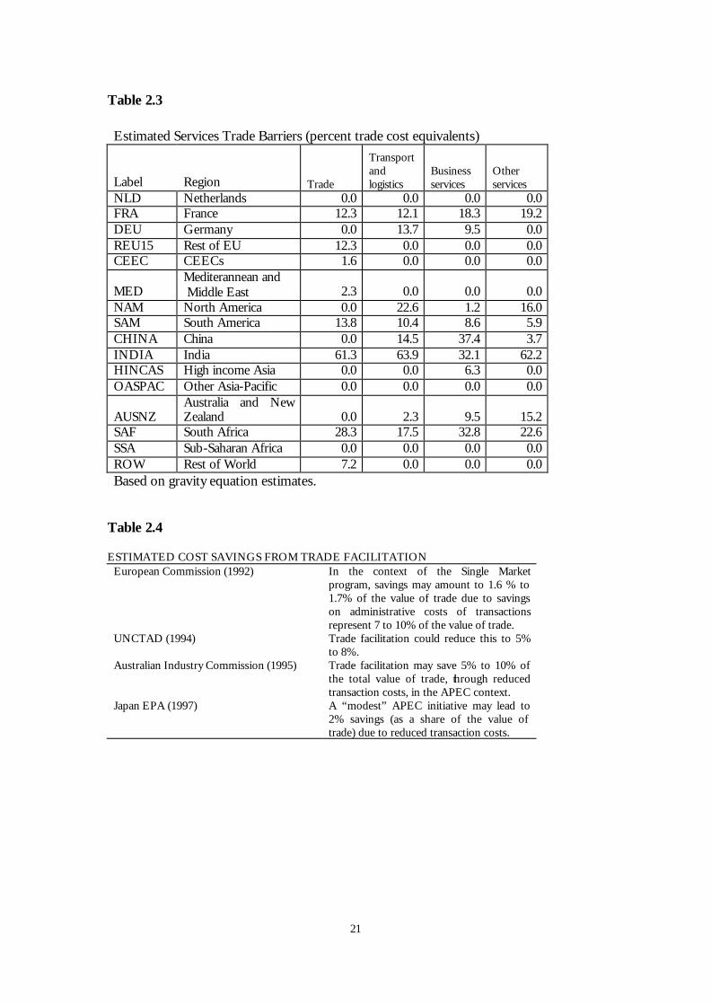
an alternative approach, we have produced estimates of "tariff equivalents" for services trade.

These are based on a simple gravity model, estimated from detailed global trade data for services

trade in 1997. The basic approach is described in an annex to this paper (available upon

request). The resulting estimates are summarized in Table 2.3. The estimates are admittedly

crude. The pattern that emerges is consistent with that for industrial tariffs. It appears that

barriers to services trade are higher (often much higher) in developing countries than in the

OECD. Hence, as in the case of industrial tariffs, the effects of further GATS negotiations will

hinge critically on developing country participation or non-participation, and the extent to which

they commit to actual liberalization rather than stand-stills (the qualitative equivalent of ceiling

bindings).

[Table 2.3 about here]

With the reduction in traditional trade barriers, attention in the regional and multilateral

trade arenas has not only shifted to quantity restrictions, but also to trade facilitation measures.

These are meant to target less transparent trade barriers, such as customs procedures, product

standards and conformance certifications, licensing requirements, and related administrative

sources of trading costs. Studies of regional integration initiatives (Baldwin and Francois 1999,

Smith and Venables 1988) have emphasized the potential for liberalization initiatives to

substantially reduce such barriers. Conceptually, these costs are different from the price and

quantity measures used for manufactures and agriculture. They are a pure global deadweight

loss.

The estimates of trading costs are very rough (at best). Nonetheless, they provide some

sense of the magnitudes involved. An overview of estimates is provided in Table 2.4. In the

context of the EC single market program, elimination of internal customs procedures and related

6

administrative streamlining were projected to reduce trading costs by up to 2 percent of the value

of trade (EC 1988). Globally, UNCTAD (1994) has noted that trading costs represent 7 to 10

percent of the cost of delivered goods. Like the EC, UNCTAD also estimates that simple trade

facilitation measures could reduce these costs by 2 percent of the value of trade. The Australian

Industry Commission (1995) has estimated potentially higher savings in the context of APEC,

ranging from 5 to 10 percent of the value of trade. Under more modest facilitation initiatives,

the Japanese Economic Planning Agency (1997) has estimated savings at 2 percent in an APEC

context, while Francois (2001) has employed a similar range of estimates.

[Table 2.4 about here]

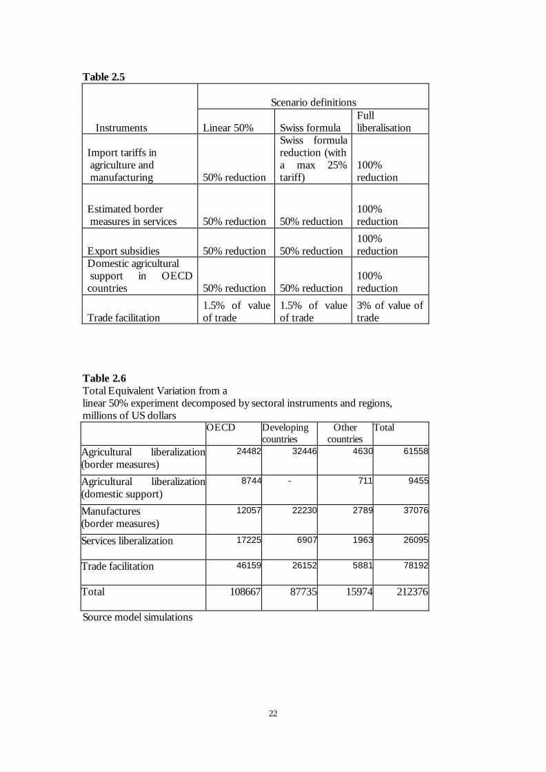
To bring these elements together, we define three sets of scenarios (See Table 2.5). The

first two are partial liberalization scenarios. In the “Linear 50%” all trade instruments are reduced

by 50%. This involves a 50% reduction in agricultural and industrial tariffs and export subsidies,

a 50% reduction in OECD domestic support for agriculture, a 50% reduction in the tariff-

equivalent of services barriers, and a partial reduction in trading costs, related to trade facilitation

measures. Services liberalization involves a 50% or a full reduction in the barriers shown in

Table 2.3. The second partial liberalization experiment is called the “Swiss formula” experiment.

In this experiment the reduction in import tariffs in agriculture and manufacture is based on a

straight Swiss formula with a coefficient of 0.25, meaning the maximum tariff is reduced to 25%.

(See Francois and Martin 2003). The third scenario simply involves full elimination of all trade

barriers. Trade facilitation, based on the range of available estimates, is assumed to range

between 1.5 percent of the value of trade (partial liberalization) and 3 percent (full liberalization).

[Table 2.5 about here]

Each experiment is decomposed, both in terms of sectors and instruments, and also in

terms of country grouping. We use the decomposition algorithm for non-linear policy

experiments outlined in Harison et al (2000). An example of the basic results structure is given

in Table 2.6, where the welfare effects (equivalent variation) are decomposed across sectoral

instruments and regions. Because of the decomposition method used, the reader can roughly

pick and choose, combining the results of hybrid experiments involving elements from different

experiments, for a rough sense of possible effects. For example, if in the next WTO round, the

outcome will be only 50% liberalization in manufactures in all regions and trade facilitation only

7

in OECD countries, the estimated world welfare effect is approximately $83 billion ($37 billion

due to liberalization in manufacturing and $46 billion due to trade facilitation in the OECD).

Finally, for each of the experiments we employ alternative model features (these model

features are discussed in more detail in section 3.2). First, we include short-run versus long-run

effects. In the short-run capital stocks are fixed and in the long-run capital stocks adjust (See

Francois et al 1997). Second, we alternatively employ perfect competition and imperfect

competition in the manufacturing and services sectors. With perfect competition we assume

constant returns to scale and with imperfect competition we assume monopolistic competition

with increasing returns to scale, firm-level product differentiation, and average cost pricing. The

model therefore includes the basic features of “economic geography” models, including

intermediate linkages, monopolistic competition, and returns from specialization. (See Francois

and Nelson 2002). For the agricultural sectors (except for the food processing industry) we

maintain constant returns to scale in all cases. We use the constant returns to scale scenario

mainly as a benchmark scenario to assess the impact of the increasing returns to scale features

and it facilitates comparison with other studies that mainly use constant returns to scale in all

sectors. A similar approach was followed in the ex-ante literature on the Uruguay Round. (See

Harrison, Rutherford, and Tarr 1997).

3. The Model and Data

We turn to a brief overview of the global computable general equilibrium (CGE) model used

here. The full set of model code, datasets, and background documentation is available for

download. [http://www.intereconomics.com/francois]. The model is characterized by an

input-output structure (based on regional and national input-output tables) that explicitly links

industries in a value added chain from primary goods, over continuously higher stages of

intermediate processing, to the final assembling of goods and services for consumption. Inter-

sectoral linkages are direct, like the input of steel in the production of transport equipment, and

indirect, via intermediate use in other sectors. The model captures these linkages by modelling

firms' use of factors and intermediate inputs. The most important aspects of the model can be

summarized as follows: (i) it covers all world trade and production; (ii) it allows for scale

economies and imperfect competition; (iii) it includes intermediate linkages between sectors; (iv)

and it allows for trade to affect capital stocks through investment effects. The last point means

we model medium to long-run investment effects. The inclusion of scale economies and

8

imperfect competition implies agglomeration effects like those emphasized in the recent

economic geography literature.

3.1 Model Data and the Benchmark

Our data come from a number of sources. Data on production and trade are based on national

social accounting data linked through trade flows (see Reinert and Roland-Holst 1997). These

social accounting data are drawn directly from the Global Trade Analysis Project (GTAP)

dataset, version 5.2. (Dimaranan and McDougall, 2002). The GTAP version 5 dataset is

benchmarked to 1997, and includes detailed national input-output, trade, and final demand

structures. The basic social accounting and trade data are supplemented with trade policy data,

including additional data on tariffs and non-tariff barriers.

The data on tariffs are taken from the WTO's integrated database, with supplemental

information from the World Bank's recent assessment of detailed pre- and post-Uruguay Round

tariff schedules and from the UNCTAD/World Bank WITS dataset. All of this tariff

information has been concorded to GTAP model sectors. Services trade barriers are based on

the gravity model estimates described in the annex to this paper (available upon request). We

also work with the schedule of China accession commitments. While the basic GTAP dataset is

benchmarked to 1997, and reflects applied tariffs actually in place in 1997, we of course want to

work with a representation of a post-Uruguay Round world. We also want to include the

accession of China, the enlargement of the EU, and Agenda 2000 reforms as part of the baseline.

To accomplish this, before conducting any policy experiments we first run a "pre-experiment" in

which we do the following:

§ implement the rest of the Uruguay Round tariff commitments,

§ implement the ATC (agreement on textiles and clothing), phasing-out quotas,

§ implement China’s accession to the WTO,

§ implement Agenda 2000,

§ and Implement the EU enlargement.

As such, the dataset we work with for actual experiments is a representation of a notional world

economy (with values in 1997 dollars) wherein we have realized many of the trade policy reforms

already programmed for the next few years.

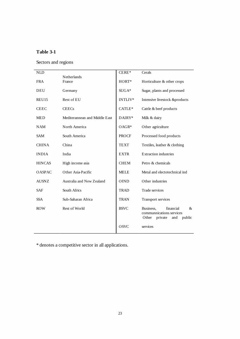
The social accounting data have been aggregated to 17 sectors and 16 regions. The

sectors and regions for the 17x16 aggregation of the data are given in Table 3.1 (a more detailed

mapping between the aggregated sectors and regions and the original GTAP regions and sectors

is given in a technical annex available with the downloadable model files).

9

3.2 Theoretical structure

We turn next to the basic theoretical features of the model. In all regions there is a single

representative, composite household in each region, with expenditures allocated over personal

consumption and savings (future consumption) and over government expenditures. The

composite household owns endowments of the factors of production and receives income by

selling them to firms. It also receives income from tariff revenue and rents accruing from

import/export quota licenses (when applicable). Part of the income is distributed as subsidy

payments to some sectors, primarily in agriculture.

On the production side, in all sectors, firms employ domestic production factors (capital,

labor and land) and intermediate inputs from domestic and foreign sources to produce outputs

in the most cost-efficient way that technology allows. Perfect competition is assumed in the

agricultural sectors as indicated in Table 3.1 (notice that the processed food products sector is

characterized by increasing returns to scale). In these sectors, products from different regions are

assumed to be imperfect substitutes in accordance with the so-called "Armington" assumption.

Production under imperfect competition is discussed below.

[Table 3.1 about here]

Prices on goods and factors adjust until all markets are simultaneously in (general)

equilibrium. This means that we solve for equilibria in which all markets clear. While we model

changes in gross trade flows, we do not model changes in net international capital flows. Rather

our capital market closure involves fixed net capital inflows and outflows. This does not

preclude changes in gross capital flows. (See the Hertel el al 1997 discussion on macroeconomic

closure. The present approach facilitates welfare analysis.) To summarize, factor markets are

competitive, and labor and capital are mobile between sectors but not between regions. All

primary factors, labor, land and capital are fully employed within each region.

We model manufacturing and services as involving imperfect competition. The

approach followed involves monopolistic competition. Monopolistic competition involves scale

economies that are internal to each firm, depending on its own production level. In particular,

based on estimates of price-cost markups, we model the sector as being characterized by

Chamberlinian large-group monopolistic competition. An important property of the

monopolistic competition model is that increased specialization at intermediate stages of

production yields returns due to specialization, where the sector as a whole becomes more

10

productive the broader the range of specialized inputs. These gains spill over through two-way

trade in specialized intermediate goods. With these spillovers, trade liberalization can lead to

global scale effects related to specialization. With international scale economies, regional welfare

effects depend on a mix of efficiency effects, global scale effects, and terms-of-trade effects.

Similar gains follow from consumer good specialization.

Another important feature involves a dynamic link, whereby the static or direct income

effects of trade liberalization induce shifts in the regional pattern of savings and investment.

These effects have been explored extensively in the trade literature, and relate to classical models

of capital accumulation and growth, rather than to endogenous growth mechanisms. Theory on

this approach includes Smith (1976, 1977) and Srinivasan and Bhagwati (1980). Several studies

of the Uruguay Round (see for example Francois, McDonald and Nordstrom 1993 and Harrison,

Rutherford and Tarr 1997) also incorporated variations on this mechanism, along with variations

in market structure. Such effects compound initial output welfare effects over the medium-run,

and can magnify income gains or losses. How much these "accumulation effects" will

supplement static effects depends on a number of factors, including the marginal product of

capital and underlying savings behaviour. It also hinges on interactions with market structure.

In the present application, we work with a classical savings-investment mechanism. This means

we model long-run linkages between changes in income, savings, and investment. The results

reported here therefore include changes in the capital stock, and the medium- to long-run

implications of such changes.

4. Results

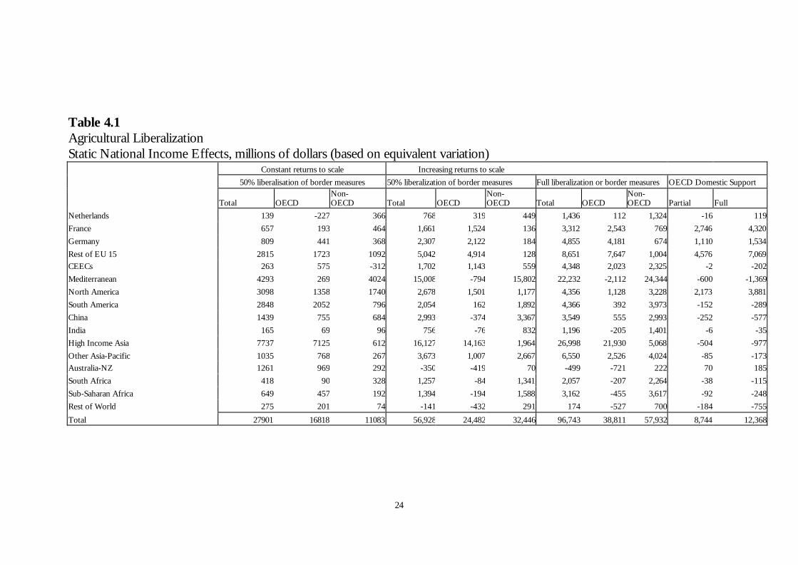
We now turn to the results of the experiments outlined in chapter two. Tables 4-1 to 4-4 present

a summary of results at the global level. The tables present a breakdown of the national income

effects (technically measured as equivalent variation) resulting from the various policy

experiments along the lines of major sector components. Table 4-1 is focused on agriculture,

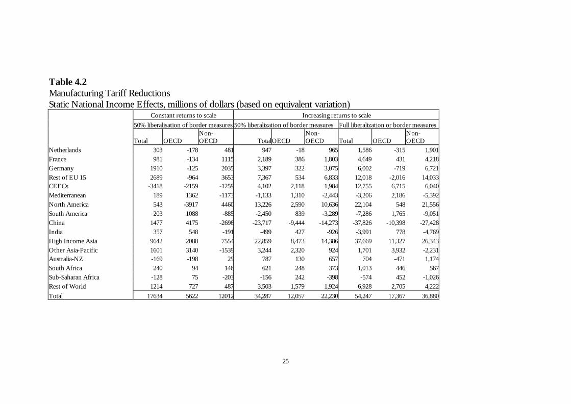
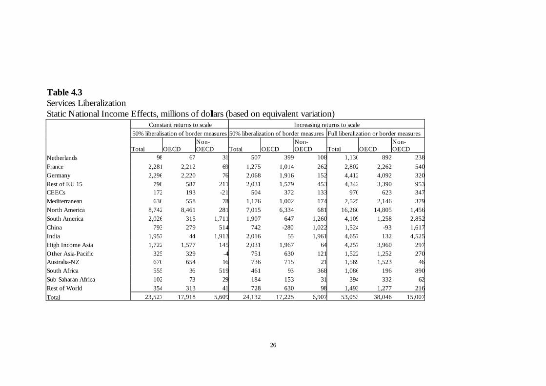
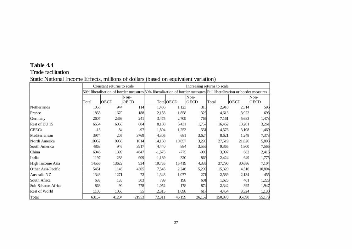
Table 4-2 is focused on manufactures, Tables 4-3 is focused on services liberalization, and Table

4-4 focuses on trade facilitation. The tables also give a breakdown of the effects of scale

economies, through a comparison of a perfect competition version of the model to the one with

scale economies and imperfect competition. We consider the increasing returns case to be the

most relevant, and unless indicated otherwise, the discussion of results pertains to this version of

the model.

[Tables 4-1,2,3,4 about here]

11

Overall, while agriculture has been a consistent sticking point in negotiations, with

agriculture exporters in particular pressing for agricultural liberalization, the overall effects are

not as clear-cut. From the set of income effect tables, we can see that agricultural liberalization

offers an uneven set of results. Liberalization of domestic support in the OECD, on the one

hand, is generally positive for the OECD, though with negative consequences for the food-

importing sub-Saharan Africa. We find that significant, though limited, liberalization yields

positive results globally, and regionally for Europe, Africa, and most of Asia. On the other hand,

on net agricultural liberalization is a mixed-bag, with gains in most areas from elimination of

domestic support, but with more mixed results from the elimination of border measures. Static

results are consistently positive if constant returns to scale (CRS) are assumed, but induced

changes in investment (not shown in all tables), combined with the imperfect competition and

agglomeration features of the model, both point to negative effects over the longer-run.

Specifically, we note the following. First, Australia and New Zealand, both net agricultural

exporters who generally favor agricultural liberalization, are not clear winners from agriculture

liberalization. In addition, the Mediterranean countries who are close to the EU and are usually

expected to gain as well from liberalization in the heavily protected EU agricultural markets are

not clear winners. In addition, other non-OECD countries (India, China, South Africa, SSA)

who do not liberalize themselves loose anyway under agricultural liberalization even as their

access to OECD markets is improved. Finally, the gains for South America are very limited

relative to expectations.

In order to understand why results and rhetoric do not necessarily match in agriculture, it

is helps to distinguish the standard perfect competition aspect of the analysis, which is held in

common with most ex-ante Doha studies use, from the additional effects related to product

differentiation and agglomeration (IRS). With IRS, expanding agricultural sectors draw resources

from industrial sectors. As a consequence, the industrial sectors have to contract, which has

negative implications for welfare because of a loss of agglomeration and variety effects. This

illustrates a point lurking in the recent literature on new economic geography and trade. If

liberalization leads to specialization and expansion of constant or decreasing returns sectors, this

may be inferior compared to the status quo or to a policy-induced expansion in IRS sectors

alongside trade liberalization. In the latter case, the traditional gains from liberalization are

magnified by agglomeration and variety effects. The pattern of results therefore highlights the

importance of taking a long-term structural view. CAIRNS group countries should perhaps be

cautious about expecting long-term economy-wide gains if, as a result of liberalization, the

12

agricultural sector draws more resources away from other productive uses. Developing countries

also need to think carefully about the risks of reinforcing an emphasis on primary exports.

The pattern for manufacturing liberalization is more consistent and generally positive,

both in the initial static results and over the long-term. From Table 4.2 the most important area

for manufacturing tariff liberalization for developing countries is the developing countries

themselves. Recall from the discussion in Section 2 that OECD tariffs are, on average, below 3

percent for manufacturing. As a result, the impact of a Swiss-formula (which targets high tariffs)

yields only limited effects on the OECD, while directly proportional cuts have a more dramatic

effect. The one region consistently, and significantly, hurt by significant manufacturing

liberalization is China. Once the WTO accession is fully implemented (as assumed in our

baseline), China will have realized most of the effects of its own trade policy reforms. Hence, the

Doha round cannot be expected to yield much additional gain in this respect. The negative

results for China follow from an erosion of its terms of trade, driven by its growth in textile

exports, combined with increased competition from other low wage countries. Natural

competitors, such as India, currently limit their participation on world markets through a mix of

import and export barriers. Rationalization in this area by developing countries leads to

heightened competition against China in a number of sectors, with the result being income losses

for China driven almost entirely by manufacturing and agricultural liberalization in the

developing world.

Another important source of overall effects is services, which yields static income gains

on a par with remaining manufacturing tariffs, and ranging potentially to over $50 billion

globally. One obvious winner from services liberalization is the United States, which is projected

to pick up a substantial share of total gains. Another big winner in services, however, is

somewhat less obvious. India, which has moved in recent years to become a major exporter in

services (including software and back office services) is projected to be a bigger potential winner

from services liberalization than North America. In fact, as a share of GDP, services is a more

important source of gains for India than agriculture and manufacturing liberalization combined.

The other important source of gains for India (and for much of the world) is trade facilitation.

In the Asia-Pacific region, where exports alone are often 50 percent of GDP, trade facilitation

yields a dramatic short-run effects as well as a long-run impact driven by investment effects

(Table 4.4). For the Asia-Pacific developing countries, the single most important issue is trade

facilitation, particularly by other developing countries.

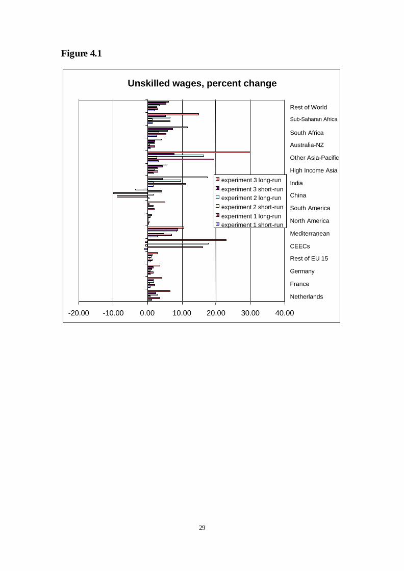
In terms of labor market effects, both unskilled and skilled workers gain from the partial

and full liberalization scenarios in most regions, except for some cases in the CEEC economies

13

and China. In China, the results are linked to the trade and income effects following from

competition with other low-wag exporters, as discussed above. The general pattern of wage

effects is summarized in Figure 4.1, which shows percent changes in wages for unskilled workers

in all regions, under all three scenarios. The basic pattern is clear – positive wage effects

everywhere, under all scenarios, except for China in all cases and the CEECs in some cases.

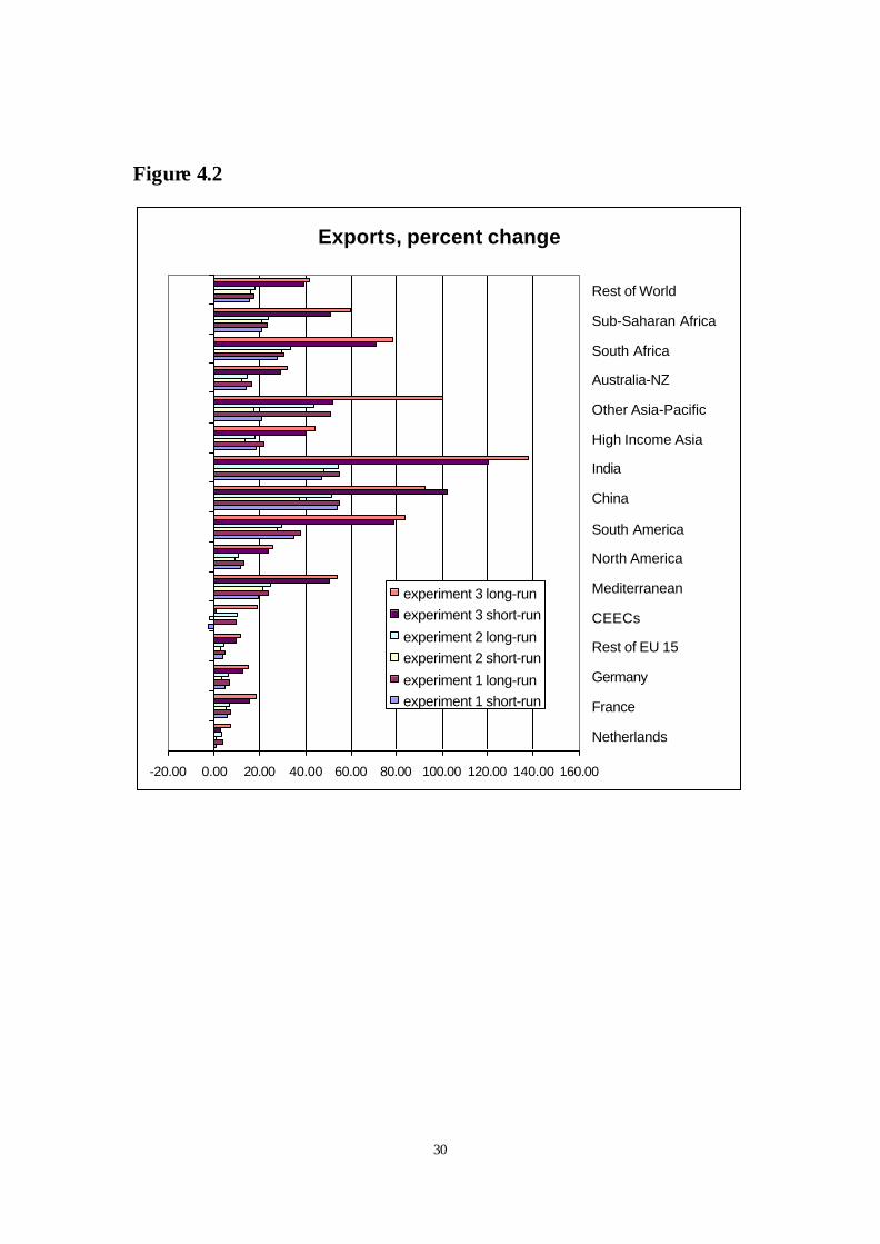
The general pattern of export effects (reported in detail in the annex tables available as

part of the model files package) is summarized in Figure 4.2. Like Figure 4.1, the emphasis here

is not on individual values, but the general pattern of results. Export growth, under all scenarios,

is greatest in the developing countries, especially in Asia and the Pacific (including India and

China), but also in the Mediterranean, African, and Latin American economies. The CEECs

suffer from trade-erosion with respect to market access to the EU15 economies. A

decomposition of bilateral trade effects shows that much of the potential gains for developing

countries depend on the realization of South-South trade opportunities. While improved access

to OECD markets is certainly important, it is equally pressing to engage in meaningful

liberalization of trade amongst developing countries. As middle-income countries are shifting

their export packages towards more processed products, the sourcing of raw materials and

intermediate inputs can increasingly take place in low-income countries.

The European Union provides a natural experiment with respect to the erosion of trade

diversion incentives in the face of multilateral liberalization. The EU is a customs union, with a

common external tariff against supplies from third countries, and practically zero tariffs within

the union. Lower external trade barriers affect producers and consumers in member states in two

related ways. First there is the direct boost to competition on home markets through improved

market access for suppliers from outside the European Union. Second, the relative position of

suppliers within the EU might change. The formation of the EU customs union leads, by

definition, to trade preferences amongst the members of the free trade area. As a consequence

the share of trade that is within the EU (intra-EU trade) is typically biased upward, and trade

within the EU is larger than might be expected on the basis of geographic proximity and other

trade promoting factors alone. With the recent eastward enlargement the preferences are

extended from the current 15 EU members to the new member states.3 Recall that the

enlargement process has been incorporated in our baseline scenario.

3 Our simulations include all 12 accession candidates newcomers, i.e. we also include Bulgaria and Romania, although these two countries will not enter the EU with the first wave of new member countries.

14

The lowering of external trade barriers by the EU will inevitably lead to the erosion of

the intra-EU trade preferences. Suppliers with lower cost will be able to enter the EU markets

once the tariff barriers have come down that currently shield domestic producers from foreign

competition. Consequently, we can expect the current bias towards intra-EU trade to be

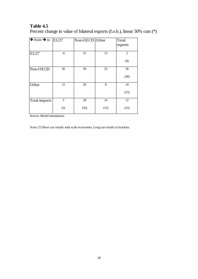
reduced. Table 4.5 illustrates this effect by breaking down the simulated change in EU27 import

values for one of the more modest liberalisation scenarios.

[Table 4.5 about here]

The 2% growth in EU27 exports is small compared to the 12% growth in world trade. A

first driver of this result is that EU countries mostly trade amongst themselves. The benefits

from removing the intra-EU barriers have already been realised in the past and there are no

additional gains for intra-EU trade in a new WTO round. A second driver of this result is the

increased competition from non-EU countries on EU markets. Simulated intra -EU27 trade

shrinks by -6% as other suppliers enter the EU markets. The most impressive growth in markets

share is realized by suppliers from developing countries, who are simulated to expand their

exports to the EU by 30%, compared to the 12% increase of imports from other developed

countries.

Because there is no positive growth to be expected from intra-EU trade, European

exports can only by increased by expansion in non-EU markets. Exports to developing countries

grow with 21% and exports to the other regions grow with 13%. Although these growth figures

are high, this is insufficient to significantly boost total exports as their weight in total EU27

exports is limited.

Developing countries obtain the highest growth in exports (30%). They expand exports

to all destinations, though the largest trade surge is observed for intra-developing country trade.

Global trade creation in this experiment amounts to 12% in the short run and 15% in the long

run. While the trade increase materialises already in the short run for the EU and other

developed economies, developing countries see even larger growth in their exports in the longer

term. Dynamic capital accumulation enables them to specialise more in exportable goods.

Trade (both exports and imports) between the EU and developing countries expands

relatively faster in our experiments than trade with developed countries. Already low trade

barriers amongst OECD countries explains this. An interesting case is Textiles and Clothing.

Recall that our experiment assumes that current quota regime, called the Agreement on Textiles

and Clothing or ATC and having grown out of the multifibre arrangement or MFA, is already

15

phased out (this is part of the baseline simulation), and the trade liberalisation experiment

subsequently lowers the import tariffs on textiles and clothing. This greatly boosts exports from

developing countries into the EU, and it crowds out the imports from developed economies and

from CEECs.

5. Conclusions

In this paper we explore the possible economic effects of the new WTO Doha Round of trade

negotiations for major developed and developing regions. Our modelling exercise includes

market structure and investment effects, and it stresses a policy benchmark including China’s

accession to the WTO, the Agenda 2000 reforms to the CAP, enlargement of the EU. The

analysis focuses on market access and agricultural support. We cover the areas of agricultural

liberalization, liberalization in industrial tariffs, liberalization in services trade, and trade

facilitation measures.

We argue that the modalities for tariff reduction are at least as important as size of cuts.

For example, in agriculture cuts in bound rates greater than 50% are required to effectively

reduce applied rates in a country like Brazil. In view of the potential impact, trade facilitation

and liberalisation in services may also need a higher valuation vis-à-vis agriculture in the current

round of negotiations. For agricultural liberalisation on the other hand, we find quite mixed

results. Given the current protection landscape, OECD countries are expected to achieve

allocative efficiency gains if they engage in own agricultural liberalisation. Reduction of domestic

support in OECD countries is certainly not unequivocally beneficial for all developing countries.

On the contrary, those developing countries that are depending on food imports, and which do

not have the resource base to develop their food sectors, will not benefit from the higher prices

brought about by liberalisation in industrial countries. In addition, for some primary exporters,

the addition of agglomeration effects in non-primary sectors highlights possible negative effects

related to primary specialization following improved market access conditions. This last point

also highlights the importance of a long-term structural view on the effects of trade liberalisation.

Even for countries with a strong natural resource base, such as the CAIRNS group, it is not

necessarily the case that expansion of primary exports is beneficial in the long run.

Finally, a key finding is the importance of effective participation by developing countries

in the negotiations, especially in manufacturing and trade facilitation. South-South trade

liberalization is key to the “development” part of the Doha Development Agenda. However, this

is downplayed in the current negotiations by all WTO-partners, with an emphasis instead on

exemptions for developing countries (called Special and Differential treatment).

16

6. References

Abreu, M. (1996), “Trade in Manufactures, the Outcome of the Uruguay Round and Developing

Country Interests,” in W. Martin and L.A. Winters (eds.), The Uruguay Round and the Developing

Countries, Cambridge University Press: Cambridge.

Baldwin, R.E. and J. Francois, "Is it time for a TRAMP? Quantitative perspectives on

transatlantic liberalization," in O.G.Mayer abd H-E Scharrer, eds., Transatlantic Relations in a

Global Economy, Hamburg: Nomos Verlagsgesellschaft, ISBN: 3-7890-5935-8, 1999, pp. 69-77.

Blackhurst, R., A. Enders and J.F. Francois, (1996)"The Uruguay Round and market access:

opportunities and challenges for developing countries," in W. Martin and A Winters, eds., The

Uruguay Round and Developing Countries, Cambridge University Press, Cambridge.

Commission of the European Communities (1988), The Cost of Non-Europe, Brussels.

Dimaranan, B. V. and R. A. McDougall, (2002). Global Trade, Assistance, and Production: The

GTAP 5 Data Base, Center for Global Trade Analysis, Purdue University.

Economic Planning Agency (1997), "Economic Effects of Selected Trade Facilitation Measures

in APEC Manila Action Plan," mimeo prepared for APEC secretariat, Japan.

Francois, J.F., (2001), THE NEXT WTO ROUND: North-South stakes in new market access

negotiations , CIES Adelaide and the Tinbergen Institute, CIES: Adelaide, ISBN: 0 86396 474 5.

Francois, J.F. and Martin, W. (2003) “Formula approaches to market access negotiations,” World

Economy: January, 1-28.

Francois, J.F., B.J. McDonald, and H. Nordstrom, (1993) "Economywide Effects of the Uruguay

Round." MTN Negotiations -- Uruguay Round background paper, GATT: Geneva, December.

Francois, J.F., B.J. McDonald, and H. Nordstrom, (1997) "Capital Accumulation in Applied

Trade Models," in J.F. Francois and K.A. Reinert, eds., Applied Methods for Trade Policy Analysis: A

Handbook, Cambridge University Press.

17

Francois, J.F. and D. Nelson, (2002) "A geometry of specialization," in The Economic Journal, June.

Francois, J.F., and D.W. Roland-Holst, (1997) "Scale Economies and Imperfect Competition," in

J.F. Francois and K.A. Reinert, eds., Applied Methods for Trade Policy Analysis: A Handbook,

Cambridge University Press.

Harrison, G.W., Tarr, D.; and Rutherford, T. F., "Quantifying the Uruguay Round," Economic

Journal, 107, September 1997, 1405-1430.

Harrison W.J., J.M. Horridge and K. Pearson (2000), Decomposing simulation results with

respect to exogenous shocks, Computational Economics, Vol. 15 , pp. 227-249.

Hathaway, D. and Ingco, M. (1996), “Agricultural Liberalization under the Uruguay Round.” In W.

Martin and A. Winters, eds, The Uruguay Round and the Developing Economies, Cambridge University

Press: New York.

Hertel, T.W. E. Ianchovichina and B.J. McDonald (1997), “Multi-Region General Equilibrium

Modeling,” in J.F. Francois and K.A. Reinert, eds., Applied Methods for Trade Policy Analysis: A

Handbook, Cambridge University Press.

Hoekman, B. (1995), "Liberalizing trade in services," in W. Martin and A. Winters, eds. The

Uruguay Round and the Developing Economies, The World Bank discussion paper 201.

Industry Commission (1995), "The Impact of APEC's Free Trade Commitment," IC95,

Australia: Canberra.

OECD (2001), Open services matter, Paris: OECD, Working party of the trade committee,

TD/TC/WP (2001)24/REV2.

Smith, A. and Venables, A.J. (1988) "Completing the Internal Market in the European

Community: Some industry simulations," European Economic Review, 32, 1501-1525.

18

Smith, M.A.M (1977), "Capital Accumulation in the Open Two-Sector Economy," The Economic

Journal 87 (June), 273-282.

Smith, M.A.M. (1976), "Trade, Growth, and Consumption in Alternative Models of Capital

Accumulation," Journal of International Economics 6, (November), 385-388.

Srinivasan, T.N. and J.N. Bhagwati (1980), "Trade and Welfare in a Steady-State," Chapter 12 in J.S.

Chipman and C.P Kindelberger, eds., Flexible Exchange Rates and the Balance of Payments, North-

Holland Publishing.

Tangermann, S. (1998), "Implementation of the Uruguay Round Agreement on Agriculture by

Major Developed Countries," in Uruguay Round Results and the Emerging Trade Agenda, UNCTAD:

Geneva.

United Nations Committee on Trade and Development (1994), "Columbus Ministerial

Declaration on Trade Efficiency."

Van Tongeren, F., H. van Meijl, Y. Surry, (2001) “Global models of trade in agriculture: a review

and assessment”, Agricultural Economics, Vol 26:2 : pp 149-172.

World Trade Organization, (2001). Ministerial Declaration, Ministerial Conference, Fourth

Session, Doha, 9-14 November 2001. Geneva: WTO, WT/MIN(01)/DEC/W/1

19

Table 2-1 Industrial tariff rates and bindings -- post UR and ITA

Percent of MFN imports that are subject to: Tariff lines bound tariffs unbound tariffs tariffs bound

above applied rates

tariffs unbound or bound above

applied rates

Share of bound duty free tariff

lines to total tar. lines

Total tariff lines

Argentina 100.0 0.0 99.9 99.9 0.0 10530 Australia 96.9 3.1 31.7 34.8 17.7 5520 Brazil 100.0 0.0 91.0 91.0 0.5 10860 Canada 99.8 0.2 45.7 45.9 34.5 6261 Chile 100.0 0.0 99.7 99.7 0.0 5055 Colombia 100.0 0.0 97.7 97.7 0.0 6145 El Salvador 97.1 2.9 96.0 98.9 0.0 4922 European Union 100.0 0.0 17.7 17.7 26.9 7635 Hungary 93.6 6.4 3.3 9.7 10.4 5896 India 69.3 30.7 14.8 45.5 0.0 4354 Indonesia 92.3 7.7 86.6 94.3 0.0 7735 Japan 95.9 4.1 0.1 4.2 47.4 7339 Korea 89.8 10.2 3.4 13.6 11.6 8882 Malaysia 79.3 20.7 31.0 51.7 1.6 10832 México 100.0 0.0 98.4 98.4 0.0 11255 New Zealand 100.0 0.0 46.5 46.5 39.5 5894 Norway 100.0 0.0 36.5 36.5 46.6 5326 Peru 100.0 0.0 98.5 98.5 0.0 4545 Phillipines 67.4 32.6 15.5 48.1 0.0 5387 Poland 92.8 7.2 44.6 51.8 2.2 4354 Singapore 36.5 63.5 11.7 75.2 15.2 4963 Sri Lanka 9.2 90.8 1.4 92.2 0.1 5933 Thailand 67.4 32.6 8.9 41.5 0.0 5244 Tunisia 67.9 32.1 41.5 73.6 0.0 5087 Turkey 49.3 50.7 0.0 50.7 1.4 15479 United States 100.0 0.0 14.0 14.0 39.4 7872 Uruguay 100.0 0.0 96.3 96.3 0.0 10530 Venezuela 100.0 0.0 90.3 90.3 0.0 5974 Zimbabwe 13.6 86.4 3.9 90.3 3.0 1929

source: Francois (2001), based on WTO and World Bank data on Uruguay Round and post-Information Technology Agreement schedules.

20

Table 2.2 Summary of Effects of Basic S wiss Formula Reductions: Applied tariffs before and after a 50% cut in average tariff bindings

Agriculture

post-UR and ITA tariffs effect of basic Swiss-formula application on tariffs

simple average

standard deviation

maximum tariff

binding overhang

simple average

standard deviation

maximum tariff

binding overhang

Percent reduction in

average European Union

5.9 7.5 74.9 0.3 3.0 2.9 10.9 0.1 -48.6

Japan 6.2 8.1 43.3 1.2 3.5 3.7 13.9 0.2 -43.0 United States 3.5 7.4 90.0 0.5 1.9 2.4 11.5 0.1 -46.6

Brazil 12.9 5.1 27.0 22.6 12.4 4.6 22.3 5.3 -3.7 India 31.0 20.8 150.0 90.7 29.5 14.9 70.8 31.3 -4.8 Thailand 26.5 14.4 65.0 7.1 15.1 6.3 30.1 1.7 -43.0

Non-agriculture

post-UR and ITA tariffs effect of basic Swiss-formula application on tariffs

simple average

standard deviation

maximum tariff

binding overhang

simple average

standard deviation

maximum tariff

binding overhang

Percent reduction in

average European Union

3.7 3.6 17.0 0.4 1.9 1.4 5.0 0.1 -47.7

Japan 2.3 3.4 30.9 0.1 1.2 1.4 5.6 0.0 -48.5 United States 3.2 4.3 37.5 0.2 1.7 1.6 6.1 0.0 -48.3

Brazil 15.9 6.0 35.0 14.9 13.5 4.2 16.7 1.9 -15.4 India 19.2 16.5 40.0 3.9 11.3 9.2 30.5 0.3 -41.3 Thailand 10.5 10.8 80.0 7.8 7.2 6.1 20.7 2.0 -31.6 Source: Francois and Martin (2003).

21

Table 2.3

Estimated Services Trade Barriers (percent trade cost equivalents)

Label Region Trade

Transport and logistics

Business services

Other services

NLD Netherlands 0.0 0.0 0.0 0.0 FRA France 12.3 12.1 18.3 19.2 DEU Germany 0.0 13.7 9.5 0.0 REU15 Rest of EU 12.3 0.0 0.0 0.0 CEEC CEECs 1.6 0.0 0.0 0.0

MED Mediterannean and Middle East 2.3 0.0 0.0 0.0

NAM North America 0.0 22.6 1.2 16.0 SAM South America 13.8 10.4 8.6 5.9 CHINA China 0.0 14.5 37.4 3.7 INDIA India 61.3 63.9 32.1 62.2 HINCAS High income Asia 0.0 0.0 6.3 0.0 OASPAC Other Asia-Pacific 0.0 0.0 0.0 0.0

AUSNZ Australia and New Zealand 0.0 2.3 9.5 15.2

SAF South Africa 28.3 17.5 32.8 22.6 SSA Sub-Saharan Africa 0.0 0.0 0.0 0.0 ROW Rest of World 7.2 0.0 0.0 0.0 Based on gravity equation estimates.

Table 2.4

ESTIMATED COST SAVINGS FROM TRADE FACILITATION European Commission (1992) In the context of the Single Market

program, savings may amount to 1.6 % to 1.7% of the value of trade due to savings on administrative costs of transactions represent 7 to 10% of the value of trade.

UNCTAD (1994) Trade facilitation could reduce this to 5% to 8%.

Australian Industry Commission (1995) Trade facilitation may save 5% to 10% of the total value of trade, through reduced transaction costs, in the APEC context.

Japan EPA (1997) A “modest” APEC initiative may lead to 2% savings (as a share of the value of trade) due to reduced transaction costs.

22

Table 2.5

Scenario definitions

Instruments Linear 50% Swiss formula Full liberalisation

Import tariffs in agriculture and manufacturing 50% reduction

Swiss formula reduction (with a max 25% tariff)

100% reduction

Estimated border measures in services 50% reduction 50% reduction

100% reduction

Export subsidies 50% reduction 50% reduction 100% reduction

Domestic agricultural support in OECD countries 50% reduction 50% reduction

100% reduction

Trade facilitation 1.5% of value of trade

1.5% of value of trade

3% of value of trade

Table 2.6 Total Equivalent Variation from a linear 50% experiment decomposed by sectoral instruments and regions, millions of US dollars OECD Developing

countries Other

countries Total

Agricultural liberalization (border measures)

24482 32446 4630 61558

Agricultural liberalization (domestic support)

8744 - 711 9455

Manufactures (border measures)

12057 22230 2789 37076

Services liberalization

17225 6907 1963 26095

Trade facilitation

46159 26152 5881 78192

Total

108667 87735 15974 212376

Source model simulations

23

Table 3-1

Sectors and regions

NLD Netherlands

CERE* Cerals

FRA France HORT* Horticulture & other crops

DEU Germany SUGA* Sugar, plants and processed

REU15 Rest of EU INTLIV* Intensive livestock &products

CEEC CEECs CATLE* Cattle & beef products

MED Mediterannean and Middle East DAIRY* Milk & dairy

NAM North America OAGR* Other agriculture

SAM South America PROCF Processed food products

CHINA China TEXT Textiles, leather & clothing

INDIA India EXTR Extraction industries

HINCAS High income asia CHEM Petro & chemicals

OASPAC Other Asia-Pacific MELE Metal and electotechnical ind

AUSNZ Australia and New Zealand OIND Other industries

SAF South Africs TRAD Trade services

SSA Sub-Saharan Africa TRAN Transport services

ROW Rest of World BSVC Business, financial & communnications services

OSVC

Other private and public

services

* denotes a competitive sector in all applications.

24

Table 4.1 Agricultural Liberalization Static National Income Effects, millions of dollars (based on equivalent variation) Constant returns to scale Increasing returns to scale 50% liberalisation of border measures 50% liberalization of border measures Full liberalization or border measures OECD Domestic Support

Total OECD Non- OECD Total OECD

Non- OECD Total OECD

Non- OECD Partial Full

Netherlands 139 -227 366 768 319 449 1,436 112 1,324 -16 119France 657 193 464 1,661 1,524 136 3,312 2,543 769 2,746 4,320Germany 809 441 368 2,307 2,122 184 4,855 4,181 674 1,110 1,534Rest of EU 15 2815 1723 1092 5,042 4,914 128 8,651 7,647 1,004 4,576 7,069CEECs 263 575 -312 1,702 1,143 559 4,348 2,023 2,325 -2 -202Mediterranean 4293 269 4024 15,008 -794 15,802 22,232 -2,112 24,344 -600 -1,369North America 3098 1358 1740 2,678 1,501 1,177 4,356 1,128 3,228 2,173 3,881South America 2848 2052 796 2,054 162 1,892 4,366 392 3,973 -152 -289China 1439 755 684 2,993 -374 3,367 3,549 555 2,993 -252 -577India 165 69 96 756 -76 832 1,196 -205 1,401 -6 -35High Income Asia 7737 7125 612 16,127 14,163 1,964 26,998 21,930 5,068 -504 -977Other Asia-Pacific 1035 768 267 3,673 1,007 2,667 6,550 2,526 4,024 -85 -173Australia-NZ 1261 969 292 -350 -419 70 -499 -721 222 70 185South Africa 418 90 328 1,257 -84 1,341 2,057 -207 2,264 -38 -115Sub-Saharan Africa 649 457 192 1,394 -194 1,588 3,162 -455 3,617 -92 -248Rest of World 275 201 74 -141 -432 291 174 -527 700 -184 -755

Total 27901 16818 11083 56,928 24,482 32,446 96,743 38,811 57,932 8,744 12,368

25

Table 4.2 Manufacturing Tariff Reductions Static National Income Effects, millions of dollars (based on equivalent variation) Constant returns to scale Increasing returns to scale 50% liberalisation of border measures 50% liberalization of border measures Full liberalization or border measures

Total OECD Non- OECD TotalOECD

Non- OECD Total OECD

Non- OECD

Netherlands 303 -178 481 947 -18 965 1,586 -315 1,901France 981 -134 1115 2,189 386 1,803 4,649 431 4,218Germany 1910 -125 2035 3,397 322 3,075 6,002 -719 6,721Rest of EU 15 2689 -964 3653 7,367 534 6,833 12,018 -2,016 14,033CEECs -3418 -2159 -1259 4,102 2,118 1,984 12,755 6,715 6,040Mediterranean 189 1362 -1173 -1,133 1,310 -2,443 -3,206 2,186 -5,392North America 543 -3917 4460 13,226 2,590 10,636 22,104 548 21,556South America 203 1088 -885 -2,450 839 -3,289 -7,286 1,765 -9,051China 1477 4175 -2698 -23,717 -9,444 -14,273 -37,826 -10,398 -27,428India 357 548 -191 -499 427 -926 -3,991 778 -4,769High Income Asia 9642 2088 7554 22,859 8,473 14,386 37,669 11,327 26,343Other Asia-Pacific 1601 3140 -1539 3,244 2,320 924 1,701 3,932 -2,231Australia-NZ -169 -198 29 787 130 657 704 -471 1,174South Africa 240 94 146 621 248 373 1,013 446 567Sub-Saharan Africa -128 75 -203 -156 242 -398 -574 452 -1,026Rest of World 1214 727 487 3,503 1,579 1,924 6,928 2,705 4,222Total 17634 5622 12012 34,287 12,057 22,230 54,247 17,367 36,880

26

Table 4.3 Services Liberalization Static National Income Effects, millions of dollars (based on equivalent variation) Constant returns to scale Increasing returns to scale 50% liberalisation of border measures 50% liberalization of border measures Full liberalization or border measures

Total OECD Non- OECD Total OECD

Non- OECD Total OECD

Non- OECD

Netherlands 98 67 31 507 399 108 1,130 892 238France 2,281 2,212 69 1,275 1,014 262 2,802 2,262 540Germany 2,296 2,220 76 2,068 1,916 152 4,412 4,092 320Rest of EU 15 798 587 211 2,031 1,579 453 4,342 3,390 953CEECs 172 193 -21 504 372 133 970 623 347Mediterranean 636 558 78 1,176 1,002 174 2,525 2,146 379North America 8,742 8,461 281 7,015 6,334 681 16,260 14,805 1,456South America 2,026 315 1,711 1,907 647 1,260 4,109 1,258 2,852China 793 279 514 742 -280 1,022 1,524 -93 1,617India 1,957 44 1,913 2,016 55 1,961 4,657 132 4,525High Income Asia 1,722 1,577 145 2,031 1,967 64 4,257 3,960 297Other Asia-Pacific 325 329 -4 751 630 121 1,522 1,252 270Australia-NZ 670 654 16 736 715 21 1,569 1,523 46South Africa 555 36 519 461 93 368 1,086 196 890Sub-Saharan Africa 102 73 29 184 153 31 394 332 62Rest of World 354 313 41 728 630 98 1,493 1,277 216Total 23,527 17,918 5,609 24,132 17,225 6,907 53,053 38,046 15,007

27

Table 4.4 Trade facilitation Static National Income Effects, millions of dollars (based on equivalent variation) Constant returns to scale Increasing returns to scale 50% liberalisation of border measures 50% liberalization of border measures Full liberalization or border measures

Total OECD Non- OECD Total OECD

Non- OECD Total OECD

Non- OECD

Netherlands 1058 944 114 1,436 1,123 313 2,910 2,314 596France 1858 1670 188 2,183 1,858 325 4,615 3,922 693Germany 2607 2366 241 3,475 2,709 766 7,161 5,683 1,478Rest of EU 15 6654 6050 604 8,188 6,431 1,757 16,462 13,201 3,261CEECs -13 84 -97 1,804 1,253 551 4,576 3,108 1,469Mediterranean 3974 205 3769 4,305 681 3,624 8,621 1,248 7,373North America 10952 9938 1014 14,150 10,857 3,293 27,519 21,626 5,893South America 4863 946 3917 4,440 884 3,556 9,365 1,800 7,565China 6046 1399 4647 -1,675 -775 -900 3,097 682 2,415India 1197 288 909 1,189 320 869 2,424 649 1,775High Income Asia 14556 13622 934 19,755 15,419 4,336 37,790 30,686 7,104Other Asia-Pacific 5451 1146 4305 7,545 2,246 5,299 15,320 4,516 10,804Australia-NZ 1343 1271 72 1,348 1,077 271 2,589 2,134 455South Africa 638 135 503 799 198 601 1,625 401 1,223Sub-Saharan Africa 868 90 778 1,052 178 874 2,342 395 1,947Rest of World 1105 1050 55 2,315 1,698 617 4,454 3,324 1,130Total 63157 41204 21953 72,311 46,159 26,152 150,870 95,690 55,179

28

Table 4.5 Percent change in value of bilateral exports (f.o.b.), linear 50% cuts (*) ê from è to EU27 Non-OECD Other Total

exports

EU27 -6 21 13 2

(4)

Non-OECD 30 39 25 30

(38)

Other 12 26 8 14

(15)

Total imports 3

(5)

28

(35)

14

(15)

12

(15)

Source: Model simulations.

Note: (*) Short run results with scale economies. Long run results in brackets.

29

Figure 4.1

Unskilled wages, percent change

-20.00 -10.00 0.00 10.00 20.00 30.00 40.00

Netherlands France

Germany Rest of EU 15 CEECs Mediterranean North America South America

China India High Income Asia Other Asia-Pacific Australia-NZ South Africa

Sub-Saharan Africa

Rest of World

experiment 3 long-run experiment 3 short-run experiment 2 long-run experiment 2 short-run experiment 1 long-run experiment 1 short-run

30

Figure 4.2

Exports, percent change

-20.00 0.00 20.00 40.00 60.00 80.00 100.00 120.00 140.00 160.00

Netherlands

France

Germany

Rest of EU 15

CEECs

Mediterranean

North America

South America

China

India

High Income Asia

Other Asia-Pacific

Australia-NZ

South Africa

Sub-Saharan Africa

Rest of World

experiment 3 long-runexperiment 3 short-run

experiment 2 long-runexperiment 2 short-run

experiment 1 long-runexperiment 1 short-run

31

Technical Annex

A.1 Introduction This annex provides an overview of the basic structure of the global CGE model employed for our assessment of Doha Round-based multilateral trade liberalization. The model is implemented in GEMPACK -- a software package designed for solving large applied general equilibrium models. The model is solved as an explicit non-linear system of equations, through techniques described by Harrison and Pearson (1994). More information can be obtained at the following URL -- http://www.monash.edu.au/policy/gempack.htm. The reader is referred to Hertel (1996: http://www.agecon.purdue.edu/gtap/model/Chap2.pdf) for a detailed discussion of the basic algebraic model structure represented by the GEMPACK code. While this appendix provides a broad overview of the model, detailed discussion of mathematical structure is limited to added features, beyond the standa rd GTAP structure.

The model is a standard multi-region computable general equilibrium (CGE) model, with important features related to the structure of competition (as described by Francois and Roland-Holst 1997). The capital accumulation mechanisms are described in Francois et al (1996b: http://www.agecon.purdue.edu/gtap/techpapr/tp-7.htm ), while imperfect competition features are described in detail in Francois (1998: http://www.agecon.purdue.edu/gtap/techpapr/tp-14.htm ). Social accounting data are based on Version 5 of the GTAP dataset (McDougal 2001), with an update to reflect post-Uruguay Round protection, Agenda 2000, China’s accession to the WTO, and EU enlargement, as discussed in the body of the report.

A.2 Overview of General Structure The general conceptual structure of a regional economy in the model is represented in Annex Figure A.1. Within each region, firms produce output, employing land, labour, capital, and natural resources and combining these with intermediate inputs. Firm output is purchased by consumers, government, the investment sector, and by other firms. Firm output can also be sold for export. Land is only employed in the agricultural sectors, while capital and labour (both skilled and unskilled) are mobile between all production sectors. Capital is fully mobile within regions. All demand sources combine imports with domestic goods to produce a composite good, as indicated in the figure. In constant returns sectors, these are Armington composites. In increasing returns sectors, these are composites of firm-differentiated goods. Relevant substitution and trade elasticities are presented in Annex Table A.1.

A.3 Taxes and policy variables Taxes are included in the theory of the model at several levels. Production taxes are placed on intermediate or primary inputs, or on output. Some trade taxes are modeled at the border. Additional internal taxes can be placed on domestic or imported intermediate inputs, and may be applied at differential rates that discriminate against imports. Where relevant, taxes are also placed on exports, and on primary factor income. Finally, where relevant (as indicated by social accounting data) taxes are placed on final consumption, and can be applied differentially to consumption of domestic and imported goods. Trade policy instruments are represented as import or export taxes/subsidies. This includes applied most-favored nation (mfn) tariffs, antidumping duties, countervailing duties, price undertakings, export quotas, and other trade restrictions. The two exceptions are service-sector trading costs, which are discussed in the next section, and agricultural quotas, discussed in the

32

subsequent section. The full set of post-Uruguay Round tariff vectors is based on Francois and Strutt (1999) and Finger et al (1998). This background paper includes a description of the methodology used to estimate post-Uruguay Round tariff rates. Post-Uruguay Round protection in agriculture is taken from GTAP estimates. The set of services trade barrier estimates is described below. Tariff rates for China’s accession to the WTO are taken from Francois and Spinanger (2001). A.4 Trade and transportation costs and services barriers International trade is modeled as a process that explicitly involves trading costs, which include both trade and transportation services. These trading costs reflect the transaction costs involved in international trade, as well as the physical activity of transportation itself. Those trading costs related to international movement of goods and related logistic services are met by composite services purchased from a global trade services sector, where the composite "international trade services" activity is produced as a Cobb-Douglas composite of regional exports of trade and transport service exports. Trade-cost margins are based on reconciled f.o.b. and c.i.f. trade data, as reported in version 5.2 of the GTAP dataset.

A second form of trade costs is known in the literature as frictional trading costs. These are implemented in the service sector. They represent real resource costs associated with producing a service for sale in an export market instead of the domestic market. Conceptually, we have implemented a linear transformation technology between domestic and export services. This technology is represented in Annex Figure A.2. The straight line AB indicates, given the resources necessary to produce a unit of services for the domestic market, the feasible amount that can instead be produced for export using those same resources. If there are not frictional barriers to trade in services, this line has slope -1. This free-trade case is represented by the line AC. As we reduce trading costs, the linear transformation line converges on the free trade line, as indicated in the figure.

The basic methodology for estimation of services barriers involves the estimation of sector-specific gravity equations, based on aggregate GTAP data (which reports detailed trading patterns in services) for total imports outside of intra-NAFTA and intra-EU trade. These equations have been estimated at the level of aggregation corresponding to the sectors of our CGE model.

The gravity equations are estimated using ordinary least squares with the following specification:

(1)

jjjjji EUaPOPaPCYaaM ε++++= 4321, where Mi,j represents imports in sector i by country j, PCYi represents per-capita income in the importing country, POP j is population, EU j is a dummy for EU countries, and ε is an error term. Deviations from predicted imports are taken as an indication of barriers to trade. These tariff equivalent rates are then backed out from a constant elasticity import demand function as follows: (2) e

MM

TT

1

0

1

0

1

=

Here, T1 is the power of the tariff equivalent (1+t1 ) such that in free trade T0 =1, and [M1/M0] is the ratio of actual to predicted imports. This is a reduced form, where actual prices and constant terms drop out because we take ratios. The term e is the demand elasticity (taken to be the substitution elasticity from Annex Table 1). Regression results from this approach are reported

33

in Annex Table A.2, while the relevant estimates of tariff equivalents for the model sectors and regions are reported in Annex Table A.3. 5. Agricultural quotas An output quota places a restriction on the volume of production. If such a supply restriction is binding, it implies that consumers will pay a higher price than they would pay in case of an unrestricted interplay of demand and supply. A wedge is created between the prices that consumers pay, PM and the marginal cost for the producer, PS. Annex Figure A.3 below illustrates this point. The vertical distance between PM and PS at quota levels is known as the tax equivalent of the quota rent. Instead of applying a quota, an equivalent level of output taxation could be administered which has the same output reducing and price increasing effect. This is illustrated by the dashed line in the figure. The shaded area indicates the value of the quota rent: the wedge between consumer and producer prices times the level of output. It is an empirical matter to determine who is actually earning the quota rent. It represents income to someone in the economy, usually the holder of the quota right, though the rent distribution depends on the institutional set-up of quota allocation and tradability.

In our model both the EU milk quota and the sugar quota are implemented at the national level. Technically, this is achieved by formulating the quota as a complementarity problem. This formulation allows for endogenous regime switches from a state when the output quota is binding to a state when the quota becomes non-binding. In addition, changes in the value of the quota rent are endogenously determined. If τ denotes the tax equivalent of the quota rent, and )( qqY −= denotes the difference between the output quota q and output q , then the complementary problem can be written as: (3) Y 0 ⊥≥τ where either

τ > 0 and Y = 0 the quota is binding or τ = 0 and Y ≥ 0 the quota is not binding Ignoring other tax and subsidy instruments that might be in place, the market price pm for commodities that are subject to a quota rent is (4) )1( τ+⋅= pspm where ps denotes the producer price, which equals marginal cost in the model. The value of the quota rent τ⋅ ps⋅ q is allocated as income to the regional household. The modelling of this class of non-continuous policy instruments has been greatly facilitated by the latest release of GEMPACK.

34

The effects of the quota, or the effect of a possible extension of quota rights, depend crucially on the size of the quota rent. For intra-EU distributional analysis it is also important to have estimates of the size of the quota rent at member state level. Such estimates are hard to obtain. Our quota rent estimates are obtained form recent studies on the EU dairy sector and sugar sector. The rent estimates for dairy are obtained from Berkhout et al. (2002), Bouamra-Mechemache et al. (2002) and Kleinhanss et al. (2002). The estimates for sugar have been obtained from Frandsen and Jensen (2002). For the Netherlands, the percentage increase of the market price above marginal productions cost, i.e. the tax equivalent of the quota rent, is estimated at 30% for milk. This is the highest figure within the EU and shows that Dutch dairy producers are very quota constrained. For sugar, France and Germany are most quota constrained, with rent estimates as high as 140%.

We have also applied milk and sugar quota in the accession candidate countries (CEECs). At the time of writing the allocation of production quota to CEEC producers is still subject to negotiations.

We have followed the suggestions of the European Commission (2002) to allocate production quota to CEECs. For milk, the EC proposes allocations based on average deliveries for direct sales during the reference period 1997-99. For sugar, this amounts to allocation based on average production in the historic reference period 1995-1999. This quota allocation allows CEECS to expand their output slightly beyond current levels, i.e. the quota is currently not binding. But it would constrain them to attain the high output levels of the pre-reform period. A.6 The composite household and final demand structure Final demand is determined by an upper-tier Cobb-Douglas preference function, which allocates income in fixed shares to current consumption, investment, and government services. This yields a fixed savings rate. Government services are produced by a Leontief technology, with household/government transfers being endogenous. The lower-tier nest for current consumption is also specified as a Cobb-Douglas. The regional capital markets adjust so that changes in savings match changes in regional investment expenditures. (Note that the Cobb-Douglas demand function is a special case of the CDE demand function employed in the standard GTAP model code. It is implemented through GEMPACK parameter files.) A.7 Market Structure

A.7.1 Demand for imports: Armington sectors

The basic structure of demand in constant returns sectors is Armington preferences. In Armington sectors, goods are differentiated by country of origin, and the similarity of goods from different regions is measured by the elasticity of substitution. Formally, within a particular region, we assume that demand goods from different regions are aggregated into a composite import according to the following CES function: (5)

j

jR

irijrij

Mrj Mq

ρρα

/1

1,,,,,

= ∑

=

In equation (5), Mj,i,r is the quantity of Mj from region i consumed in region r. The elasticity of substitution between varieties from different regions is then equal to σM

j , where σMj=1/(1-ρj).

Composite imports are combined with the domestic good qD in a second CES nest, yielding the Armington composite q.

35

(6) ( ) ( )[ ] jjj DrjrDj

MrjrMjrj qqq

βββ /1

,,,,.., Ω+Ω= The elasticity of substitution between the domestic good and composite imports is then equal to σD

j, where σDj=1/(1-β j). At the same time, from the first order conditions, the demand for

import Mj,i,r can then be shown to equal (7)

( ) Mrj

Mrj

rij

rij

Mrj

R

irijrij

rij

rijrij

EPP

EPP

M

Mj

Mj

Mj

Mj

mi

,1

,,,

,,

,

1

1

1,,,,

,,

,,,,

\

−

−

=

−

=

= ∑

σσ

σσ

σ

α

αα

where EM

j,r represents expenditures on imports in region r on the sector j Armington composite. In practice, the two nests can be collapsed, so that imports compete directly with each other and with the corresponding domestic product. This implies that the substitution elasticities in equations (1) and (2) are equal. (These elasticities are reported in Annex Table 1).

A.7.2 Imperfect competition

As indicated in Annex Table A.1, we model manufacturing sectors and service sectors as being imperfectly competitive. The approach we follow has been used in the Michigan and the WTO assessment of the Uruguay Round. Recent model testing work indicates that this approach works “best” vis-à-vis Armington models, when tracked against actual trade patterns. (See Fox 1999, who uses the U.S.-Canada FTA as a natural experiment for model testing).

Formally, within a region r, we assume that demand for differentiated intermediate products belonging to sector j can be derived from the following CES function, which is now indexed over firms or varieties instead of over regions. We have

(8) j

jn

irijrijrj Xq

Γ

=

Γ

= ∑

/1

1,,,,, γ

where γj,i,r is the demand share preference parameter, Xj,i,r is demand for variety i of product j in region r, and σj = 1/(1-Γj) is the elasticity of substitution between any two varieties of the good. Note that we can interpret q as the output of a constant returns assembly process, where the resulting composite product enters consumption and/or production. Equation (8) could therefore be interpreted as representing an assembly function embedded in the production technology of firms that use intermediates in production of final goods, and alternatively as representing a CES aggregator implicit in consumer utility functions. In the literature, and in our model, both cases are specified with the same functional form. While we have technically dropped the Armington assumption by allowing firms to differentiate products, the vector of γ parameters still provides a partial geographic anchor for production. (Francois and Roland-Holst 1997, Francois 1998).

36

Globally, firms in different regions compete directly. These firms are assumed to exhibit monopolistically competitive behaviour. This means that individual firms produce unique varieties of good or service j, and hence are monopolists within their chosen market niche. Given the demand for variety, reflected in equation (8), the demand for each variety is less than perfectly elastic. However, while firms are thus able to price as monopolists, free entry (at least in the long-run) drives their economic profits to zero, so that pricing is at average cost. The joint assumptions of average cost pricing and monopoly pricing, under Bertrand behaviour, imply the following conditions for each firm fi in region i: (9)

−−

∑∑PP

X

X =

r f, j,

r k, j,1

r ,f j,

r k, j,n

1=k

1

f j,

r ,f j,R

1=rf j,

j

i

j

i

i

i

σσ

αα

ζ

(10) AC = P i f,i f,

The elasticity of demand for each firm fi will be defined by the following conditions. (11) ζσσε i f, j,jji f, j, )(1 + = −

(12) ε i f,i f,

i f,i f, 1=

PMCP

In a fully symmetric equilibrium, we would have ζ=n-1. However, the calibrated model includes CES weights γ , in each regional CES aggregation function, that will vary for firms from different regions. Under these conditions, ζ is a quantity weighted measure of market share. To close the system for regional production, we index total resource costs for sector j in region i by the resource index Z. Full employment of resources hired by firms in the sector j in region i then implies the following condition.

(13) TC = Z f i, j,

n

1=fi j,

i

∑

Cost functions for individual firms are defined as follows: (14) P )x b + a( = )xC( Zi j,i j,i j,i j, i j,

This specification of monopolistic competition is implemented under the “large group” assumption, which means that firms treat the variable n as "large", so that the perceived elasticity of demand equals the elasticity of substitution. The relevant set of equations then collapses to the following:

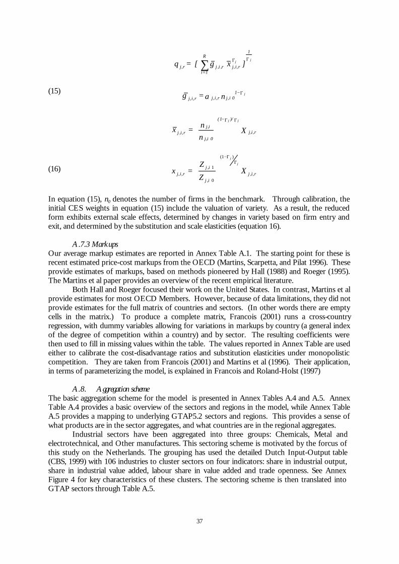
37

(15)

X nn = x

n =

]x [ = q

r i, j,0i j,

i j,

)/(1

rij

0i j,1

r i, j,rij

rijrij

R

1=i

1

r j,

jj

j

j j

ΓΓ−

Γ−

Γ Γ

∑

,,

,,

,,,,

αγ

γ

(16) rij

ij

ijrij X

Z

Zx

j

j

,,

)1(

0,

1,,,

ΓΓ−

=

In equation (15), n0 denotes the number of firms in the benchmark. Through calibration, the initial CES weights in equation (15) include the valuation of variety. As a result, the reduced form exhibits external scale effects, determined by changes in variety based on firm entry and exit, and determined by the substitution and scale elasticities (equation 16).

A.7.3 Markups Our average markup estimates are reported in Annex Table A.1. The starting point for these is recent estimated price-cost markups from the OECD (Martins, Scarpetta, and Pilat 1996). These provide estimates of markups, based on methods pioneered by Hall (1988) and Roeger (1995). The Martins et al paper provides an overview of the recent empirical literature.

Both Hall and Roeger focused their work on the United States. In contrast, Martins et al provide estimates for most OECD Members. However, because of data limitations, they did not provide estimates for the full matrix of countries and sectors. (In other words there are empty cells in the matrix.) To produce a complete matrix, Francois (2001) runs a cross-country regression, with dummy variables allowing for variations in markups by country (a general index of the degree of competition within a country) and by sector. The resulting coefficients were then used to fill in missing values within the table. The values reported in Annex Table are used either to calibrate the cost-disadvantage ratios and substitution elasticities under monopolistic competition. They are taken from Francois (2001) and Martins et al (1996). Their application, in terms of parameterizing the model, is explained in Francois and Roland-Holst (1997)

A.8. Aggregation scheme

The basic aggregation scheme for the model is presented in Annex Tables A.4 and A.5. Annex Table A.4 provides a basic overview of the sectors and regions in the model, while Annex Table A.5 provides a mapping to underlying GTAP5.2 sectors and regions. This provides a sense of what products are in the sector aggregates, and what countries are in the regional aggregates.

Industrial sectors have been aggregated into three groups: Chemicals, Metal and electrotechnical, and Other manufactures. This sectoring scheme is motivated by the forcus of this study on the Netherlands. The grouping has used the detailed Dutch Input-Output table (CBS, 1999) with 106 industries to cluster sectors on four indicators: share in industrial output, share in industrial value added, labour share in value added and trade openness. See Annex Figure 4 for key characteristics of these clusters. The sectoring scheme is then translated into GTAP sectors through Table A.5.

38

Annex References Berkhout, J.F.M.Helming, F.W. van Tongeren, P., C.van Bruchem, A.J.de Kleijn (2002), Zuivelbeleid zonder melkquotering? Mogelijke gevolgen voor Nederland en de EU. The Hague:LEI report no. 6.02.003. (Dairy policy without quota: impact on The Netherlands the EU) Bouamra-Mechemache, Z. V. Requillart , A.Burrell, H. Guyomard and R. Jongeneel (2002), “The INRA-Wageningen simulation system for the EU dairy sector”. Paper presented at the Xth EAAE congress, Zaragoza, Spain. European Commission (2002), Enlargemet and Agriculture. Successfully integrating the new member states into the CAP. Issues paper, Brussels, (January). Ethier, W. (1982), “National and International Returns to Scale in the Modern Theory of International Trade,” American Economic Review, 72 (June), 950-959. Finger, J.M., U. Reincke, and M. Ingco (1996), The Uruguay Round: Statistics on Tariff Concessions Given and Received, World Bank: Washington. Fox, Alan K. (1999), "Evaluating the Success of a CGE Model of the Canada -U.S. Free Trade Agreement," presented at The Second Annual Conference in Global Economic Analysis, June 20-22. Francois, J.F., THE NEXT WTO ROUND: North-South stakes in new market access negotiations , CIES Adelaide and the Tinbergen Institute, CIES: Adelaide, 2001. ISBN: 086396 474 5. Francois, J.F. (1998), "Scale economies and imperfect competition in the GTAP model," GTAP consortium technical paper. Francois, J.F., B. McDonald and H. Nordstrom (1996b), "Trade liberalization and the capital stock in the GTAP model," GTAP consortium technical paper. Francois, J.F. and D.W. Roland-Holst (1997), "Scale economies and imperfect competition, in Francois,J.F. and K.A. Reinert, eds. (1997), Applied methods for trade policy analysis: a handbook, Cambridge University Press: New York. Francois, J.F. and D. Spinanger (2001), “Greater China’s Accession to the WTO: Implications for International Trade/Production and for Hong Kong,” paper prepared for the Hong Kong Trade Development Council, December. Francois, J.F. and A. Strutt (1999), "Post Uruguay Round Tariff Vectors For GTAP Version 4," Erasmus University manuscript. Frandsen, S. and H. Jensen (2002), Reforming the EU sugar policy, Paper presented at the Xth EAAE congress, Zaragoza, Spain. Hall, R.E. (1988), "The relation between price and marginal cost in U.S. industry", Journal of Political Economy, Vol. 96, No. 5, pp. 921-947.

39

Hertel 1996 Hertel, T., ed., (1996), Global Trade Analysis, Cambridge University Press: Cambridge MA. Kleinhanss, W., D. Manegold, M. Bertelsmeier, E. Deeken, E. Giffhorn, P. Jägersberg, F. Offermann, B. Osterburg, P. Salamon (2002),” How to phase out milk quotas - Possible impacts on European and German agriculture “, Paper presented at the Xth EAAE congress, Zaragoza, Spain. Laird, S. (1998), ‘Multilateral Approaches to Market Access Negotiations,” WTOTPRD staff working paper TPRD-98-02, Geneva. Martins, J.O., Scarpetta, S. and D. Pilat (1996), " Mark-Up Ratios In Manufacturing Industries Estimates For 14 OECD Countries," OECD Economics Department Working Paper No. 162. McDougall, R., ed. (2001). The GTAP database -- version 5, Global Trade Analysis Center: Purdue University. Roeger, W. (1995), "Can Imperfect Competition explain the Difference between Primal and Dual Productivity Measures? Estimates for US manufacturing", Journal of Political Economy, Vol. 103, No. 2, pp. 316-330.

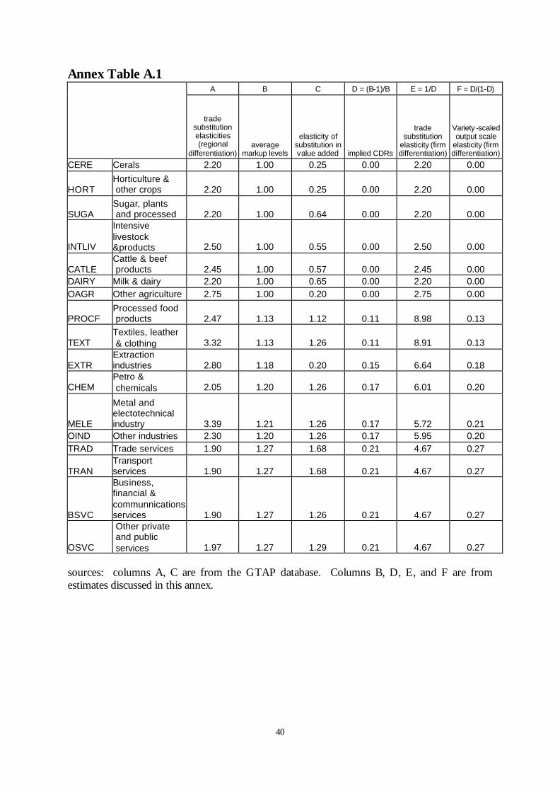
40

Annex Table A.1 A B C D = (B-1)/B E = 1/D F = D/(1-D)

trade substitution elasticities (regional

differentiation) average

markup levels

elasticity of substitution in value added implied CDRs

trade substitution

elasticity (firm differentiation)

Variety -scaled output scale

elasticity (firm differentiation)

CERE Cerals 2.20 1.00 0.25 0.00 2.20 0.00

HORT Horticulture & other crops 2.20 1.00 0.25 0.00 2.20 0.00

SUGA Sugar, plants and processed 2.20 1.00 0.64 0.00 2.20 0.00

INTLIV

Intensive livestock &products 2.50 1.00 0.55 0.00 2.50 0.00

CATLE Cattle & beef products 2.45 1.00 0.57 0.00 2.45 0.00

DAIRY Milk & dairy 2.20 1.00 0.65 0.00 2.20 0.00 OAGR Other agriculture 2.75 1.00 0.20 0.00 2.75 0.00

PROCF Processed food products 2.47 1.13 1.12 0.11 8.98 0.13

TEXT Textiles, leather & clothing 3.32 1.13 1.26 0.11 8.91 0.13

EXTR Extraction industries 2.80 1.18 0.20 0.15 6.64 0.18

CHEM Petro & chemicals 2.05 1.20 1.26 0.17 6.01 0.20

MELE

Metal and electotechnical industry 3.39 1.21 1.26 0.17 5.72 0.21

OIND Other industries 2.30 1.20 1.26 0.17 5.95 0.20 TRAD Trade services 1.90 1.27 1.68 0.21 4.67 0.27

TRAN Transport services 1.90 1.27 1.68 0.21 4.67 0.27

BSVC

Business, financial & communnications services 1.90 1.27 1.26 0.21 4.67 0.27

OSVC

Other private and public services 1.97 1.27 1.29 0.21 4.67 0.27

sources: columns A, C are from the GTAP database. Columns B, D, E, and F are from estimates discussed in this annex.

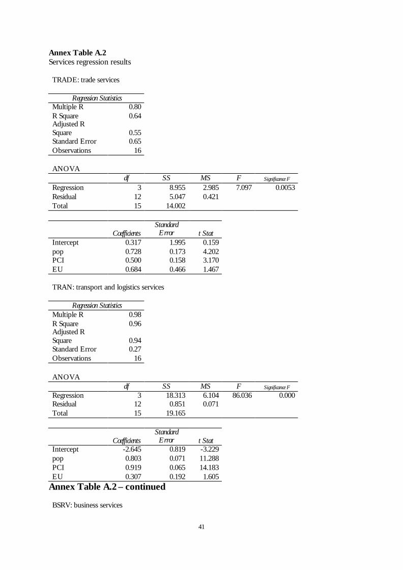
41

Annex Table A.2 Services regression results TRADE: trade services

Regression Statistics Multiple R 0.80 R Square 0.64 Adjusted R Square 0.55 Standard Error 0.65 Observations 16 ANOVA

df SS MS F Significance F

Regression 3 8.955 2.985 7.097 0.0053 Residual 12 5.047 0.421 Total 15 14.002

Coefficients Standard

Error t Stat Intercept 0.317 1.995 0.159 pop 0.728 0.173 4.202 PCI 0.500 0.158 3.170 EU 0.684 0.466 1.467 TRAN: transport and logistics services

Regression Statistics Multiple R 0.98 R Square 0.96 Adjusted R Square 0.94 Standard Error 0.27 Observations 16 ANOVA

df SS MS F Significance F Regression 3 18.313 6.104 86.036 0.000 Residual 12 0.851 0.071 Total 15 19.165

Coefficients Standard

Error t Stat Intercept -2.645 0.819 -3.229 pop 0.803 0.071 11.288 PCI 0.919 0.065 14.183 EU 0.307 0.192 1.605

Annex Table A.2 – continued BSRV: business services

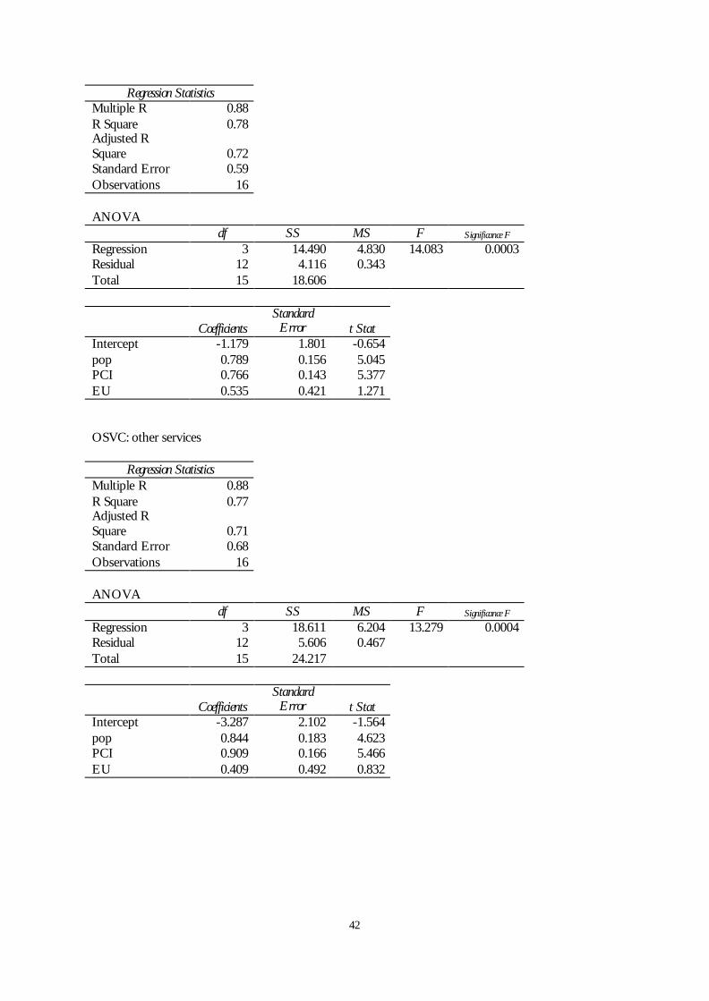
42

Regression Statistics Multiple R 0.88 R Square 0.78 Adjusted R Square 0.72 Standard Error 0.59 Observations 16 ANOVA

df SS MS F Significance F Regression 3 14.490 4.830 14.083 0.0003 Residual 12 4.116 0.343 Total 15 18.606

Coefficients Standard

Error t Stat Intercept -1.179 1.801 -0.654 pop 0.789 0.156 5.045 PCI 0.766 0.143 5.377 EU 0.535 0.421 1.271 OSVC: other services

Regression Statistics Multiple R 0.88 R Square 0.77 Adjusted R Square 0.71 Standard Error 0.68 Observations 16 ANOVA

df SS MS F Significance F Regression 3 18.611 6.204 13.279 0.0004 Residual 12 5.606 0.467 Total 15 24.217

Coefficients Standard

Error t Stat Intercept -3.287 2.102 -1.564 pop 0.844 0.183 4.623 PCI 0.909 0.166 5.466 EU 0.409 0.492 0.832

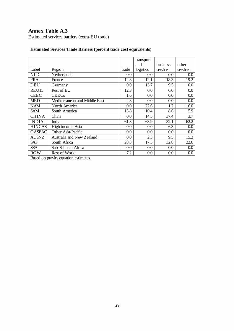
43

Annex Table A.3 Estimated services barriers (extra-EU trade) Estimated Services Trade Barriers (percent trade cost equivalents)

Label Region trade

transport and logistics

business services

other services

NLD Netherlands 0.0 0.0 0.0 0.0 FRA France 12.3 12.1 18.3 19.2 DEU Germany 0.0 13.7 9.5 0.0 REU15 Rest of EU 12.3 0.0 0.0 0.0 CEEC CEECs 1.6 0.0 0.0 0.0 MED Mediterranean and Middle East 2.3 0.0 0.0 0.0 NAM North America 0.0 22.6 1.2 16.0 SAM South America 13.8 10.4 8.6 5.9 CHINA China 0.0 14.5 37.4 3.7 INDIA India 61.3 63.9 32.1 62.2 HINCAS High income Asia 0.0 0.0 6.3 0.0 OASPAC Other Asia-Pacific 0.0 0.0 0.0 0.0 AUSNZ Australia and New Zealand 0.0 2.3 9.5 15.2 SAF South Africa 28.3 17.5 32.8 22.6 SSA Sub-Saharan Africa 0.0 0.0 0.0 0.0 ROW Rest of World 7.2 0.0 0.0 0.0 Based on gravity equation estimates.

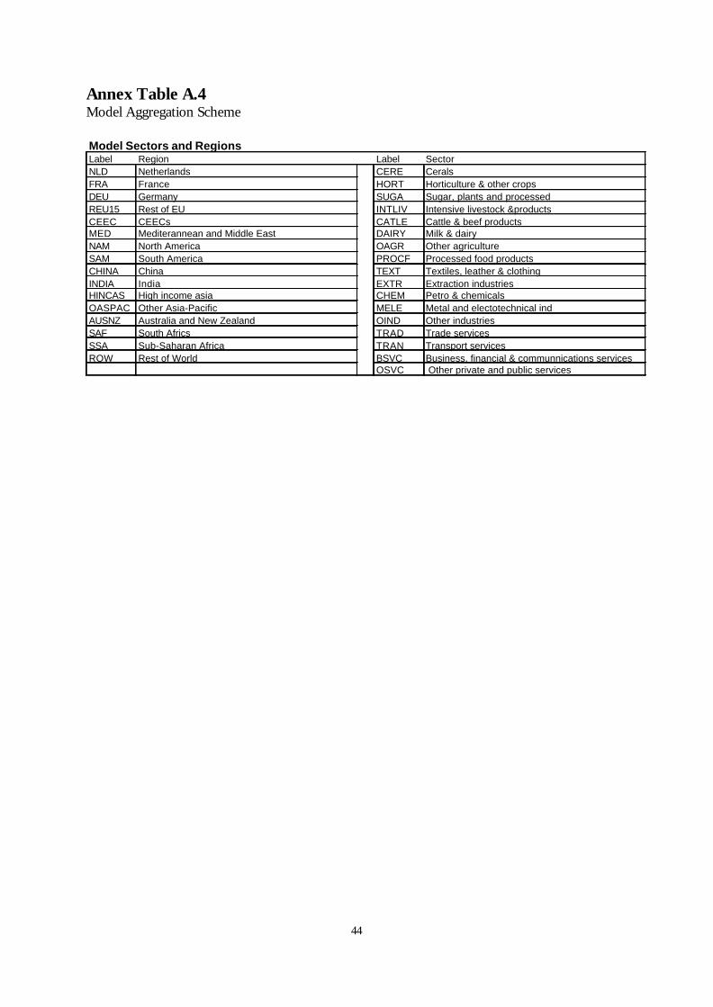
44

Annex Table A.4 Model Aggregation Scheme Model Sectors and RegionsLabel Region Label SectorNLD Netherlands CERE CeralsFRA France HORT Horticulture & other cropsDEU Germany SUGA Sugar, plants and processedREU15 Rest of EU INTLIV Intensive livestock &productsCEEC CEECs CATLE Cattle & beef productsMED Mediterannean and Middle East DAIRY Milk & dairyNAM North America OAGR Other agricultureSAM South America PROCF Processed food productsCHINA China TEXT Textiles, leather & clothingINDIA India EXTR Extraction industriesHINCAS High income asia CHEM Petro & chemicalsOASPAC Other Asia-Pacific MELE Metal and electotechnical indAUSNZ Australia and New Zealand OIND Other industriesSAF South Africs TRAD Trade servicesSSA Sub-Saharan Africa TRAN Transport servicesROW Rest of World BSVC Business, financial & communnications services

OSVC Other private and public services

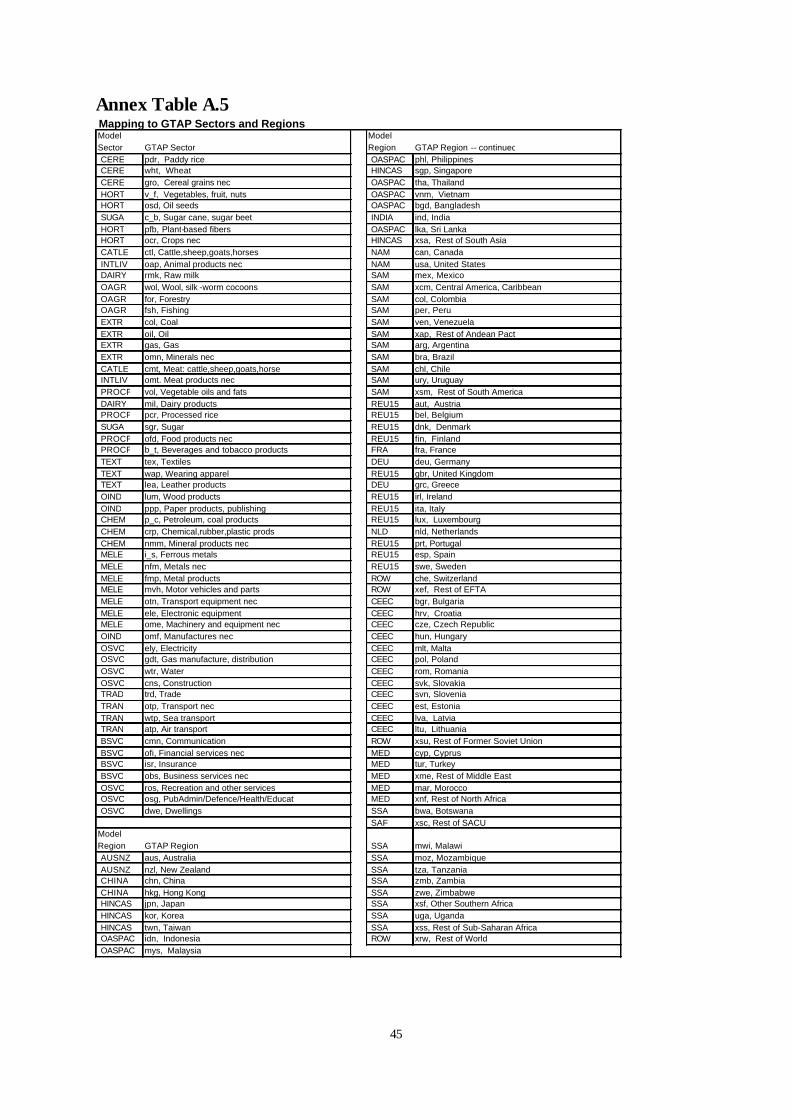
45

Annex Table A.5 Mapping to GTAP Sectors and Regions Model Sector GTAP Sector

Model Region GTAP Region -- continued

CERE pdr, Paddy rice OASPAC phl, Philippines CERE wht, Wheat HINCAS sgp, Singapore CERE gro, Cereal grains nec OASPAC tha, Thailand HORT v_f, Vegetables, fruit, nuts OASPAC vnm, Vietnam HORT osd, Oil seeds OASPAC bgd, Bangladesh SUGA c_b, Sugar cane, sugar beet INDIA ind, India HORT pfb, Plant-based fibers OASPAC lka, Sri Lanka HORT ocr, Crops nec HINCAS xsa, Rest of South Asia CATLE ctl, Cattle,sheep,goats,horses NAM can, Canada INTLIV oap, Animal products nec NAM usa, United States DAIRY rmk, Raw milk SAM mex, Mexico OAGR wol, Wool, silk -worm cocoons SAM xcm, Central America, Caribbean OAGR for, Forestry SAM col, Colombia OAGR fsh, Fishing SAM per, Peru EXTR col, Coal SAM ven, Venezuela EXTR oil, Oil SAM xap, Rest of Andean Pact EXTR gas, Gas SAM arg, Argentina EXTR omn, Minerals nec SAM bra, Brazil CATLE cmt, Meat: cattle,sheep,goats,horse SAM chl, Chile INTLIV omt. Meat products nec SAM ury, Uruguay PROCF vol, Vegetable oils and fats SAM xsm, Rest of South America DAIRY mil, Dairy products REU15 aut, Austria PROCF pcr, Processed rice REU15 bel, Belgium SUGA sgr, Sugar REU15 dnk, Denmark PROCF ofd, Food products nec REU15 fin, Finland PROCF b_t, Beverages and tobacco products FRA fra, France TEXT tex, Textiles DEU deu, Germany TEXT wap, Wearing apparel REU15 gbr, United Kingdom TEXT lea, Leather products DEU grc, Greece OIND lum, Wood products REU15 irl, Ireland OIND ppp, Paper products, publishing REU15 ita, Italy CHEM p_c, Petroleum, coal products REU15 lux, Luxembourg CHEM crp, Chemical,rubber,plastic prods NLD nld, Netherlands CHEM nmm, Mineral products nec REU15 prt, Portugal MELE i_s, Ferrous metals REU15 esp, Spain MELE nfm, Metals nec REU15 swe, Sweden MELE fmp, Metal products ROW che, Switzerland MELE mvh, Motor vehicles and parts ROW xef, Rest of EFTA MELE otn, Transport equipment nec CEEC bgr, Bulgaria MELE ele, Electronic equipment CEEC hrv, Croatia MELE ome, Machinery and equipment nec CEEC cze, Czech Republic OIND omf, Manufactures nec CEEC hun, Hungary OSVC ely, Electricity CEEC mlt, Malta OSVC gdt, Gas manufacture, distribution CEEC pol, Poland OSVC wtr, Water CEEC rom, Romania OSVC cns, Construction CEEC svk, Slovakia TRAD trd, Trade CEEC svn, Slovenia TRAN otp, Transport nec CEEC est, Estonia TRAN wtp, Sea transport CEEC lva, Latvia TRAN atp, Air transport CEEC ltu, Lithuania BSVC cmn, Communication ROW xsu, Rest of Former Soviet Union BSVC ofi, Financial services nec MED cyp, Cyprus BSVC isr, Insurance MED tur, Turkey BSVC obs, Business services nec MED xme, Rest of Middle East OSVC ros, Recreation and other services MED mar, Morocco OSVC osg, PubAdmin/Defence/Health/Educat MED xnf, Rest of North Africa OSVC dwe, Dwellings SSA bwa, Botswana

SAF xsc, Rest of SACU Model Region GTAP Region SSA mwi, Malawi AUSNZ aus, Australia SSA moz, Mozambique AUSNZ nzl, New Zealand SSA tza, Tanzania CHINA chn, China SSA zmb, Zambia CHINA hkg, Hong Kong SSA zwe, Zimbabwe HINCAS jpn, Japan SSA xsf, Other Southern Africa HINCAS kor, Korea SSA uga, Uganda HINCAS twn, Taiwan SSA xss, Rest of Sub-Saharan Africa OASPAC idn, Indonesia ROW xrw, Rest of World OASPAC mys, Malaysia

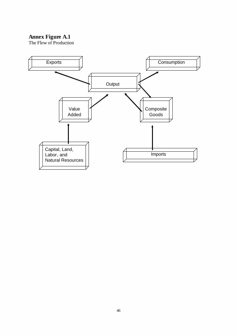
46

Annex Figure A.1 The Flow of Production

Output

ValueAdded

CompositeGoods

ImportsCapital, Land, Labor, and Natural Resources

Exports Consumption

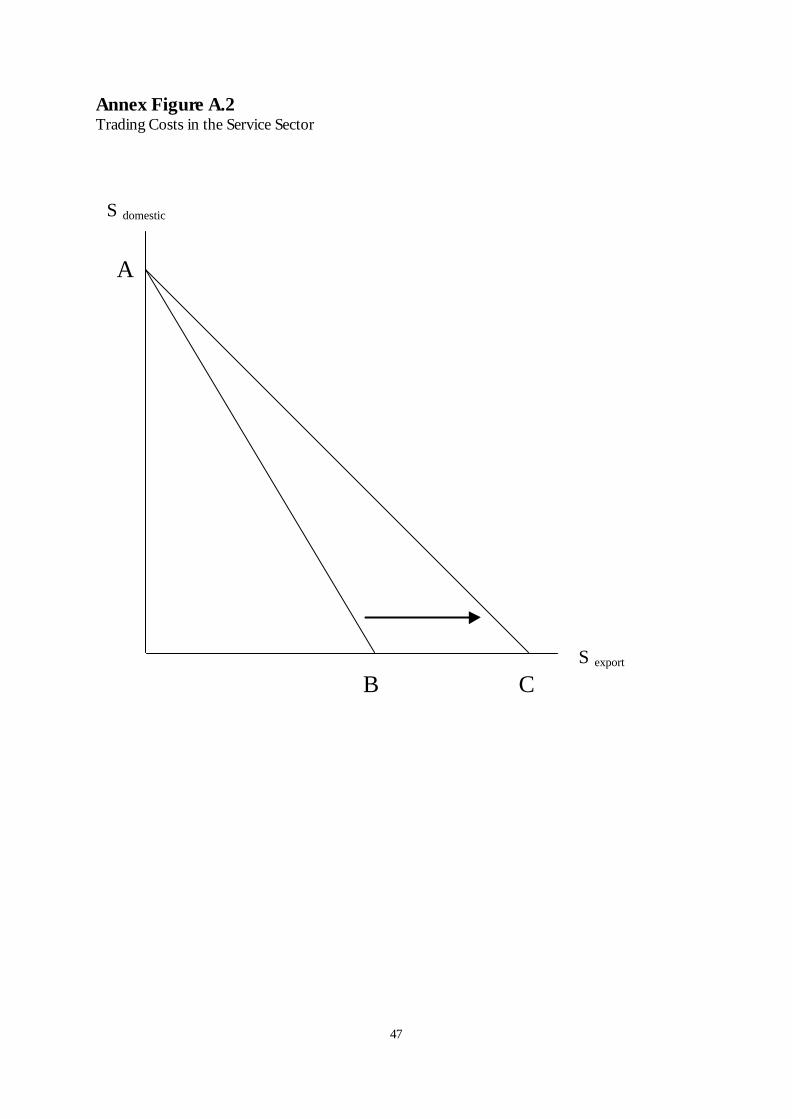
47

Annex Figure A.2 Trading Costs in the Service Sector

S domestic

S export

A

B C

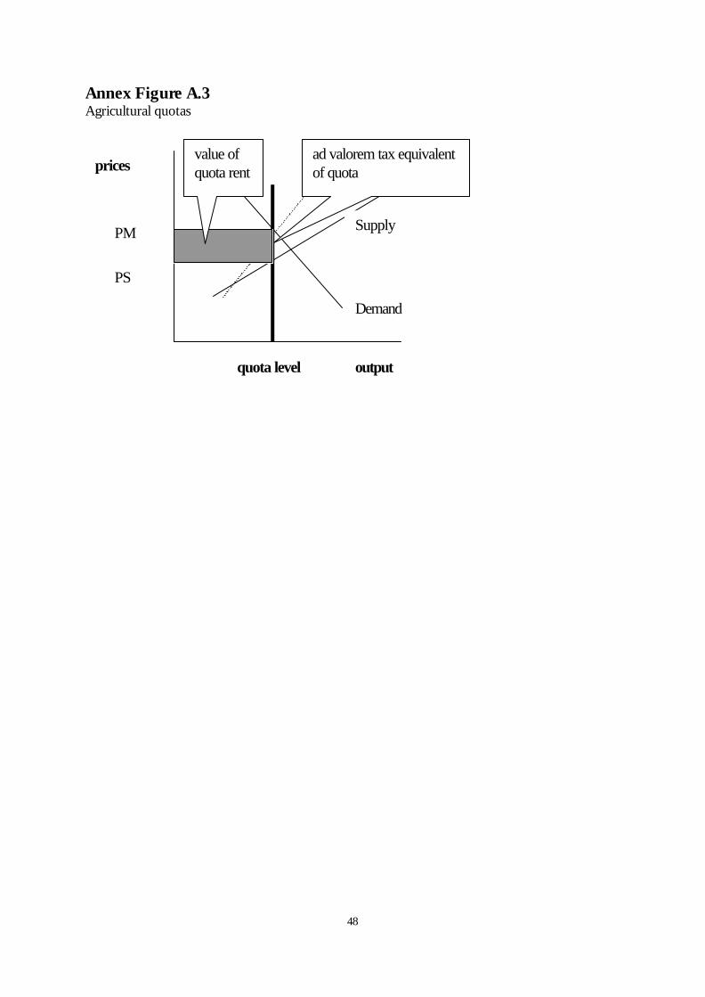
48

Annex Figure A.3 Agricultural quotas

PM

PS

output quota level

prices

Supply

Demand

value of quota rent

ad valorem tax equivalent of quota