Trade, Merchants, andthe Lost Cities of the Bronze Age∗

Gojko Barjamovic † Thomas Chaney‡ Kerem Coşar§ Ali Hortaçsu¶

March 17, 2017PRELIMINARY AND INCOMPLETE: DO NOT CIRCULATE.

Abstract

We analyze a large dataset of commercial records produced by Assyrian merchants in the19th Century BCE. Using the information collected from those records, we estimate a structuralgravity model of long-distance trade in the Bronze Age. We find a distance elasticity for ancienttrade close to modern estimates. We also use our structural gravity model to locate lost ancientcities. In many instances, our structural estimates confirm the conjecture of historians whofollowed a radically different method. In some instances, our estimates confirm one conjectureagainst others. Finally, using historical data on political centers, as well as modern data onregional trade and incomes, we document persistent patterns in cities’ prominence across fourmillennia even after controlling for time-invariant geographic attributes such as agricultural suit-ability, mineral resources and defensive ability. Discussing related quantitative and qualitativeevidence from historical geography, we argue that the locational advantage brought by naturaltransport routes dictated by topography is a key factor in explaining the persistence of city sizedistributions.

∗This research is supported by the University of Chicago Neubauer Collegium for Culture and Society. ThomasChaney acknowledges ERC grant N°337272–FiNet for financial support. Daniel Ehrlich, Simon Fuchs and Joonhwi Jooprovided excellent research assistance. We are grateful to Adam Grant Anderson, Thomas Hertel, Alessio Palmisanofor valuable discussions and sharing their data, and to participants at Neubauer Collegium workshops, CEPR ERWIT2016 conference and various presentations for comments and suggestions.

†Harvard University, barjamovic@fas.harvard.edu.‡Sciences Po and CEPR, thomas.chaney@gmail.com.§University of Virginia and CEPR, keremcosar@gmail.com.¶University of Chicago and NBER, hortacsu@gmail.com.

This paper analyzes a vast collection of commercial records from the earliest documented long-

distance trade in world history: The Old Assyrian trade network connecting northern Iraq, northern

Syria and central Turkey during the Middle Bronze Age period (c. 1945-1730 BCE). The clay

tablets on which the merchants inscribed their shipment consignments, expenses, and contracts

—excavated, translated and published by archaeologists and historians for more than a century—

paint a rich picture of an exchange economy.

Originating from the city of Aššur on the West bank of the River Tigris, some 100 km south

of the modern-day Iraqi city of Mosul, a few hundred Assyrian merchants settled in Kanesh on a

permanent or temporary basis. They maintained smaller expatriate trading settlements in some

40 urban centers on the central Anatolian Plateau and Northern Syria. Kanesh was the regional

hub of the overland commodity trade involving the import of luxury fabrics and tin from Aššur to

copper rich Anatolia in exchange for silver and gold. Assyrian merchants were also involved in a

voluminous trade of copper and wool within Anatolia itself.

Our first contribution is to extract systematic information on commercial linkages between cities

from ancient texts. To do so, we use two complementary approaches. This first method leverages

the fact that the ancient records we study can be transcribed into the Latin alphabet and Arabic

numbers, allowing all texts to be digitized and parsed. We automatically search for joint mentions

of city pairs across all records. Since those records all come from merchants’ archives, and primarily

deal with business matters, we take a joint mention of two cities in a text as evidence of some

economic interaction between them. The second method involves systematic reading of texts, which

requires an intimate knowledge of the Assyrian dialect of the ancient Akkadian language that the

records are written in. Taking individual source context into account, this analysis relies exclusively

upon a smaller set of records that explicitly refer to journeys between cities and distinguishes

whether the specific journey was undertaken for the purpose of moving cargo, return journeys, or

journeys undertaken for other reasons (legal, private, etc.).

Our second contribution is to estimate a structural gravity model of ancient trade. We build

a simple Ricardian model of trade in precious commodities. Further imposing that bilateral trade

frictions can be summarized by a power function of geographic distance, our model makes predictions

on the number of transactions between city pairs, as in our data. Our model can be estimated solely

on bilateral trade flows data and on the geographic location of at least some cities. Our structural

estimate for the distance elasticity of trade, -1.47, is surprisingly close to modern estimates.

Our third contribution is to use our structural gravity model to estimate the geographic location

of lost cities. While some of the cities in which the Assyrian merchants settled have been located

2

and excavated by contemporary scholarship, most of the places mentioned in the records can not

be securely identified with a place on a modern map and are now lost to us. Analyzing the records

for descriptions of trade and routes connecting the cities and the landscapes surrounding them,

historians have developed qualitative conjectures about potential locations of several of these lost

cities. We propose an alternative, quantitative method based on maximizing the fit of the gravity

equation. We show that as long as we have data on trade between known and lost cities, with

sufficiently many known compared to lost cities, a structural gravity model is able to estimate the

likely geographic coordinates of lost cities. Our framework not only provides point estimates for the

location of lost cities, but also confidence regions around those point estimates. For a majority of

the lost cities, our quantitative estimates come remarkably close to the qualitative conjectures pro-

duced by historians, corroborating both such historical models and our purely quantitative method.

Moreover, in some cases where historians disagree on the likely location of a lost city, our quantita-

tive method supports the conjecture of some historians and rejects that of others, with the promise

of settling some debates among historians.

Our fourth contribution is to test for the persistence of economic forces over a long horizon. Aside

from allowing us to recover the location of lost cities, our gravity models yields a structural estimate

for the fundamental economic size of ancient cities. No reliable data on production and consumption,

or even population size or density in the 19th Century BC survives. We infer city sizes instead from

the propensity of those cities to trade with others in a structural equilibrium trade model. Projecting

these ancient city sizes on a set of time-invariant, observable local amenities and resources, such as

crop yields, elevation, ruggedness, proximity to waterways or natural resources, we do not find any

robust relationship. Estimated ancient city sizes are, however, strongly correlated with the political

importance of those cities in the subsequent four millennia, as well as the economic size of those

cities in the current era (based on trade within Turkish cities in 2014), even after controlling for

these geographic attributes. At face value, these findings support the hypothesis that the spatial

distribution of economic activity may be driven by random factors or early advantages that persists

over very long periods through path-dependence and lock-in effects, while local fixed factors may

play a secondary role. In light of quantitative and qualitative evidence from historical geography,

however, we argue that a factor usually overlooked by economists, natural transportation networks

shaped by the topography of the wider region, is a critical factor in explaining the hierarchy of

ancient cities and their modern counterparts.

3

Related literature. Our paper contributes to several literatures. First, we provide the oldest

estimate for the distance elasticity of trade, dating back to 19th century BCE. This precedes the

available estimates going back to the mid-19th century CE by about four millennia (Disdier and

Head, 2008). Second, we invert the structural gravity framework in order to locate lost cities,

complementing qualitative approaches in history and archeology with a quantitative method rooted

in economic theory. We improve on an earlier contribution by Tobler and Wineburg (1971) in

that we use a much larger dataset on bilateral economic interactions between cities, and flexibly

estimate the distance elasticity jointly with the coordinates of lost cities, while they imposed a

quadratic distance elasticity. Finally, we provide novel evidence on the drivers of city sizes. An

important line of theoretical and empirical inquiry in economic geography involves attempts at

explaining the discrepancies in the economic and demographic size of cities observed at any point in

time. First-nature forces, i.e., locational fundamentals as dictated by geography, is potentially an

important factor (Davis and Weinstein, 2002). Second-nature forces, i.e., agglomeration of economic

activity for non-geographic reasons, may magnify these discrepancies or generate size differentials

even across seemingly homogenous locations (Krugman, 1991). Finally, path-dependence through

lock-in effects could lead to the persistence of past factors—related to the fundamentals that may

have been important once (Bleakley and Lin, 2012; Michaels and Rauch, 2016), or to random events

such as the quality of governance at some point in history. Our results and historical setting suggest

that centrality in transport routes dictated by topography may be an important geographic factor

in explaining persistence of cities’ long-run economic fortunes.

The remainder of the paper is organized as follows. Section 1 describes our data. Section

2 derives our model and our estimation strategy. Section 3 presents the results of our structural

estimation. Section 4 assesses the role of local geographic factors in explaining city sizes, and section

5 tests for the long-run persistence in cities’ economic outcomes.

1 Ancient Trade Data

Our data comes from a collection of around 13,000 texts that constitute the conserved and edited art

of around 23,500 texts excavated primarily at the archaeological site of Kültepe, ancient Kanesh,

located in Turkey’s central Anatolian province of Kayseri. These texts were inscribed on clay

tablets in the Akkadian language in cuneiform script by ancient Assyrian merchants, their families

and business partners. The texts date back to a period between 1945 and 1730 BCE, with around

90% of the sample belonging to just one generation of traders, c. 1910 - 1880 BCE.

4

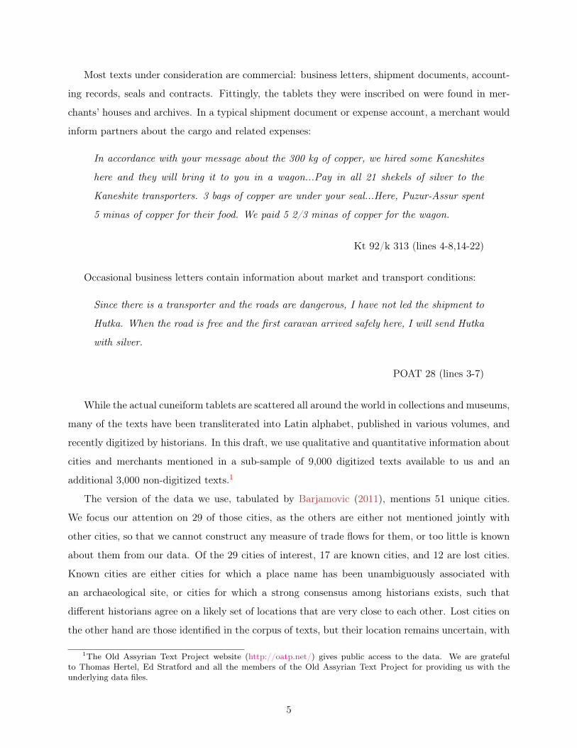
Most texts under consideration are commercial: business letters, shipment documents, account-

ing records, seals and contracts. Fittingly, the tablets they were inscribed on were found in mer-

chants’ houses and archives. In a typical shipment document or expense account, a merchant would

inform partners about the cargo and related expenses:

In accordance with your message about the 300 kg of copper, we hired some Kaneshites

here and they will bring it to you in a wagon...Pay in all 21 shekels of silver to the

Kaneshite transporters. 3 bags of copper are under your seal...Here, Puzur-Assur spent

5 minas of copper for their food. We paid 5 2/3 minas of copper for the wagon.

Kt 92/k 313 (lines 4-8,14-22)

Occasional business letters contain information about market and transport conditions:

Since there is a transporter and the roads are dangerous, I have not led the shipment to

Hutka. When the road is free and the first caravan arrived safely here, I will send Hutka

with silver.

POAT 28 (lines 3-7)

While the actual cuneiform tablets are scattered all around the world in collections and museums,

many of the texts have been transliterated into Latin alphabet, published in various volumes, and

recently digitized by historians. In this draft, we use qualitative and quantitative information about

cities and merchants mentioned in a sub-sample of 9,000 digitized texts available to us and an

additional 3,000 non-digitized texts.1

The version of the data we use, tabulated by Barjamovic (2011), mentions 51 unique cities.

We focus our attention on 29 of those cities, as the others are either not mentioned jointly with

other cities, so that we cannot construct any measure of trade flows for them, or too little is known

about them from our data. Of the 29 cities of interest, 17 are known cities, and 12 are lost cities.

Known cities are either cities for which a place name has been unambiguously associated with

an archaeological site, or cities for which a strong consensus among historians exists, such that

different historians agree on a likely set of locations that are very close to each other. Lost cities on

the other hand are those identified in the corpus of texts, but their location remains uncertain, with

1The Old Assyrian Text Project website (http://oatp.net/) gives public access to the data. We are gratefulto Thomas Hertel, Ed Stratford and all the members of the Old Assyrian Text Project for providing us with theunderlying data files.

5

no definitive answer from archaeological evidence. From the analysis of textual evidence and the

topography of the region, historians have developed competing theories about potential locations

for some of those lost cities. We propose to use data on bilateral commercial interactions between

known and lost cities and a structural gravity model to inform the search for those lost cities.

We construct three measures of bilateral commercial interactions between cities. The texts also

contain qualitative information about prices, financial contracts and resolution of legal disputes,

which we do not use but hope to analyze in future work.

The first measure is a count of all mentions of actual cargo shipments from i to j in tablets,

N cargoij ≡ # of mentions of cargo traveling from i to j.

To construct this measure, we systematically read and translated all tablets. All mentions of cargo

shipments in the text were identified. A typical letter will describe one or several itineraries of cargo

shipments. The following is an excerpt from a memorandum on travel expenses describing several

cargo trips. City names are underlined:

From Durhumit until Kanesh I incurred expenses of 5 minas of refined (copper), I spent

3 minas of copper until Wahšušana, I acquired and spent small wares for a value of 4

shekels of silver.

Kt 91/k 424 (lines 24-29)

From this sentence, we identify three shipments: from Durhumit to Kanesh, from Kanesh to

Wahšušana and from Durhumit to Wahšušana. Note that for itineraries of the type A → B → C,

we count three trips, A → B, A → C and B → C. As we only very rarely have a description of

the content of the caravans, we are unable to identify the intensive margin of shipments, i.e., the

value of the wares being transported. Instead, we measure the extensive margin, simply counting

the number of shipments. In total, from reading through about 12,000 texts, we extract 253 unique

tablets with explicit shipping details, from which we identify 318 shipments.

The total number of shipments we can identify is unfortunately too small, and bilateral flows

between cities contains too many zeros to identify our model. As a consequence, we add to these

shipments additional information about merchants’ travels as our second measure. We count all

mentions of actual travels of individuals from i to j in tablets,

N travelij ≡ # of mentions of persons traveling from i to j.

6

This includes not only caravans transporting cargo, as in our first measure N cargo, but also travels

of individuals which may not be directly involved in shipping goods. So by construction, N cargo ⊂

N travel. The following letter sent to the Assyrian port authorities at Kanesh from its emissaries at

the Assyrian port in Wahšušana describes how missives sent from Wahšušana to Purušhaddum will

travel by two different routes, presumably during a conflict, so as to ensure safe arrival:

To the Port Authorities of Kanesh from your envoys and the Port Authorities of Wahšušana.

We have heard the tablets that the Station(s) in Ulama and Šalatuwar have brought us,

and we have sealed them and (hereby) convey them on to you. On the day we heard

the tablets, we sent two messengers by way of Ulama and two messengers by way of

Šalatuwar to Purušhaddum to clear the order. We will send you the earlier message that

they brought us so as to keep you informed. The Secretary Ikun-pıya is our messenger.

Kt 83/k 117 (lines 1-24)

From this letter, we identify 9 trips: fromUlama toWahšušana and from Šalatuwar toWahšušana

(the letters received by the emissaries); from Wahšušana to Ulama, from Ulama to Purušhaddum

and from Wahšušana Purušhaddum (the first messengers); from Wahšušana to Šalatuwar, from

Šalatuwar to Purušhaddum and from Wahšušana to Purušhaddum (the second messengers); from

Wahšušana to Kanesh (the message expected to be forwarded in the near future). We do not count

the first mention of a trip from Wahšušana to Kanesh (the actual and forwarded letters sent by the

emissaries): Most of our data comes from letters found in merchants’ archives in the city of Kanesh.

By construction, all those letters involve a trip to Kanesh as the letter is being sent. Counting those

trips would systematically bias our measures in favor of finding large inflows into Kanesh. As with

N cargoij , for itineraries of the type A→ B → C, we count three trips involving all downstream pairs.

While the information in N travel is not necessarily about actual shipment of goods, it informs us

about a broader set of economic interactions. As our data comes from letters between merchants,

if N travelij is large, we infer that flows of trade, services and people from i to j are large. Mentions

of persons’ travels adds 87 trips to the 318 shipments of Xcargo, for a total of 299 itineraries and

405 trips (itineraries that involve more than two cities generate multiple trips).

The third measure is a simple automated count of all joint attestations of cities i and j in our

9,000 digitized tablets,

N jointij ≡ # of joint attestations of cities i and j.

7

If cities A, B and C are mentioned jointly in a given tablet, no matter how many times each, we

count one joint attestation between A and B, one between A and C, and one between B and C. We

use all possible spellings of city names.2 We extract a total of 944 joint attestations of city pairs.

These joint attestations may be about a specific shipment from one city to the another, about a

merchant traveling between cities, about a financial contract involving parties in different cities, or

simply about a letter mentioning those cities for different reasons. While this measure may pick

up economically irrelevant linkages between cities, the benefit from using this measure is two-fold.

First, this measure is automated, allowing us to quickly extract large amounts of information at

little cost, without the need to painstakingly read through thousands of ancient texts. Measurement

error is traded off by the mere quantity of information and the efficacy of extracting it. Second,

this measure complements our other measures, adding information about potentially meaningful

economic interactions that a direct human read of the texts would not systematically pick up. For

instance, a financial contract which involves counterparts in cities i and j would not count into

our other measures N cargo and N travel, although it informs us about a direct economic interaction

between agents in i and j.

While the data for N cargo and N travel are collected using a qualitative method —reading through

the texts and understanding their meaning— very different from the method used for N joint —au-

tomatically searching for co-occurrences— those measures are correlated. For instance, we find a

62% correlation between N travel and N joint.

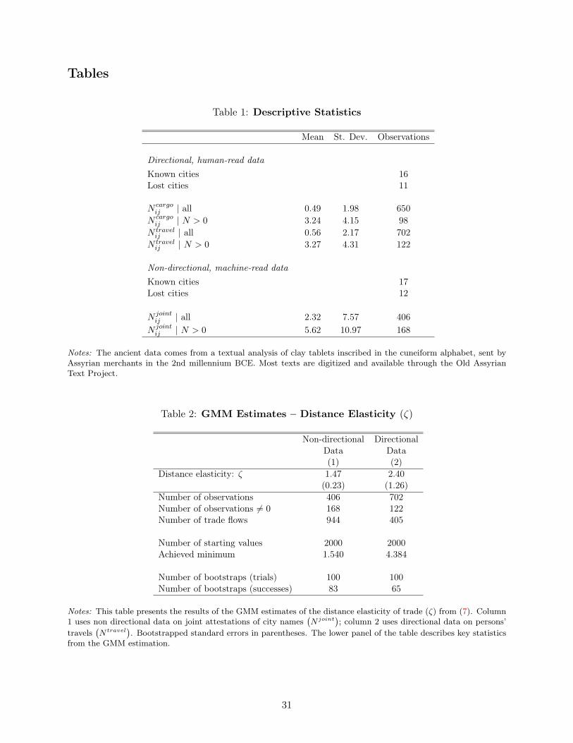
Table 1 provides summary statistics for the ancient data. Note that by only counting meaningful

economic ties, the human-read data eliminates one known and one lost city from the analysis. The

mean number of travels across all city pairs is 0.56. As in the modern international trade data,

many city pairs do not trade: of all the 702 potential export-import relationships (directional ij and

ji pairs of 27 cities), only 122 have a positive flow. Average N travel for these trading pairs is 3.27.

As expected, the machine-read non-directional data N joint contains a higher number of bilateral

links since it does not distinguish coincidental co-occurrences of cities in texts from business-related

travels between them.

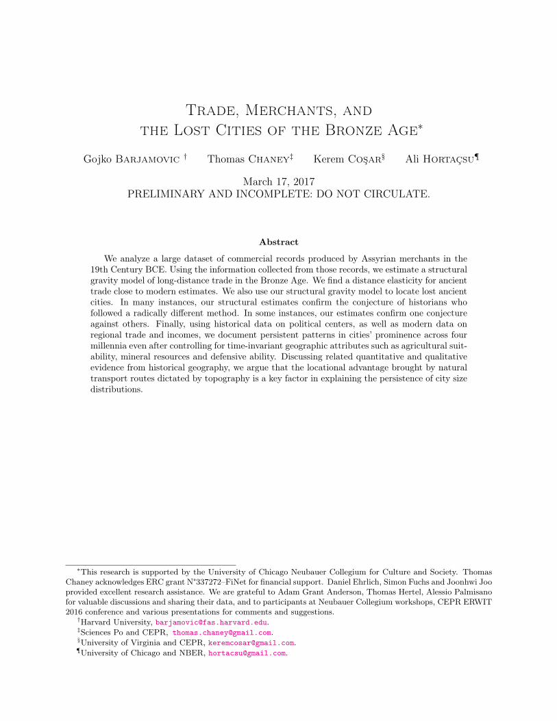
Figure 1 plots the map of cities, including a preview of estimated locations from both data sets.

The city of Kanesh, marked K, is geographically central to the system of cities under study. As

discussed above, it was also the operational center of Assyrian merchants in central Anatolia. Trade

2We exclude Aššur, the capital city of the Assyrians, from our automated search for two reasons: First, Aššur,is also the name of the main Assyrian deity, and is used as the word for a calendar month; second, the city of Aššuris often referred to as simply “the city." Our automated search is not able to use a letter’s context to distinguishbetween Aššur as a goddess, as a month, or as a city; or the word for “city” as being Aššur or another city.

8

flows, however, do not just display a hub-spoke structure around Kanesh, as seen by the rich pattern

of bilateral ties between cities in figure C.1.

2 Model and Estimation

We build a simple model of trade in which merchants arbitrage price differentials between cities.

While stylized, this model captures key features of trade in the Bronze Age. For instance, the

model can accommodate a commodity produced outside of our network of trading cities, such as tin

sourced from Central Asia, traded locally among Assyrian colonies, and exported to distant places

such as Egypt. We also make every effort to characterize equilibrium quantities in our model with

direct counterparts in our dataset, such as the count of transactions instead of their value.

Model. We follow Eaton and Kortum (2002) closely. There are K + L cities, K of them known,

and L of them lost. Tradable commodities (tin, copper, wool...) are indexed by ω. Merchants

arbitrage price differentials between cities, subject to bilateral transaction costs. For simplicity, we

assume iceberg ad valorem transaction costs, such that delivering one unit of a good from city i to

city j requires shipping τij ≥ 1 units of the good, while the remaining fraction 1 − 1/τij is lost in

transit. If a merchant observes a cost ci in a city i, and a cost cj in city j, such that

τijci < τjjcj ,

she can exploit an arbitrage opportunity: Buy τij units of the good at a cheap cost τijci in i, ship

them to j, and sell at a high cost τjjcj for a profit.3 We assume the cost of producing one unit of

any commodity ω in city i, in any period, follows a Weibull distribution,

Pr [ci (ω) ≤ c] = 1− exp(−Ticθ

). (1)

The cost ci (ω) includes both the marginal cost of production, but also any markup over marginal

cost. The distribution of costs is i.i.d across commodities and over time, and costs are independent

across cities. θ > 0 is an inverse measure of the dispersion of costs. Ti > 0 is a measure of the

3As the merchants we consider are mobile, constantly traveling between cities themselves, we do not considerthe problem of repatriating the proceeds from this sale explicitly. In particular, we implicitly assume repatriation ofprofits is costless. If repatriating profits entails a cost, the τij term would contain both the cost of shipping goodsand of repatriating profits. We also explicitly assume a transaction cost even for within city transactions, τjj ≥ 1, tocapture local distribution costs.

9

fundamental “size” of city i.4

Similar to Eaton and Kortum (2002), the equilibrium price for commodity ω in city j—with

merchants arbitraging away cost differences between cities—is the lowest cost among all possible

sources, pj (ω) = mini {τijci (ω)}. The distribution of prices in city j is then Weibull with shape

parameter θ and scale parameter∑

i′ Ti′τ−θi′j . The unconditional probability that a good sourced

from city i is purchased in city j is

πij = Pr

[τijci ≤ min

i′

{τi′jci′

}]=

Tiτ−θij∑

i′ Ti′τ−θi′j

. (2)

Observe that more productive cities, i.e., those with higher T , are also more likely to ship goods to

other destinations. To close the model, we further assume the total number of buyers in city j, each

buying one unit per period, is proportional to the city’s productivity, Tj .5 With N i.i.d. draws for

the costs {ci (ω)}i, the expected number of shipments going from i to j is

E [Nij ] = N · πijTj = N ·TiTjτ

−θij∑

i′ Ti′τ−θi′j

. (3)

Estimation. Our empirical strategy is to use the theory-implied expected number of shipments

in equation (3) to estimate the structural parameters of the model and the geographic location of

lost cities.

To proceed, we parametrize the symmetric trade cost function as

τ−θij = Distance−ζij , ∀i, j, (4)

where we normalize internal distances, Distanceii = 30km, capturing the economic hinterland of a

city within the reach of a day’s travel at the time. For cities i and j with latitude-longitude (ϕi, λi)4For instance, following Kortum (1997), if the distribution of efficiency for producing commodity ω locally is

Pareto with shape parameter θ, and if the probability that any local worker/entrepreneur tries her luck operating alocal facility producing ω is exponentially distributed, then the cost of producing good ω in city i (the inverse of theefficiency) is distributed according to the Weibull distribution (1), where Ti is exactly proportional to the number oflocal households and their efficiency. With Weibull distributed costs, larger and/or more efficient cities, in the senseof cities with a higher Ti, will also be cities with lower costs on average:

Ei [c] ∝ T−1/θi .

This model can also accommodate cases where good ω is not produced locally, but instead is sourced from outsideour network of K +L trading cities and enters our system only through the gateway city i (e.g. tin mined in CentralAsia, and shipped to Aššur,). In that case, Ti depends both on the fundamental productivity of local producers in i,T locali , on the productivity of outside producers sending goods to i, T outsidei , and on the cost of sourcing goods fromoutside, τoutside,i,

Ti = τ−θii Tlocali + τ−θoutside,iT

outsidei .

5This assumption is consistent with the general equilibrium Ricardian model of Eaton and Kortum (2002),Armington model of Anderson and van Wincoop (2003), or monopolistic model of Krugman (1980).

10

and (ϕj , λj), we let Distanceij = H (ϕi, λi;ϕj , λj) , where the function H maps geo-coordinates

into geographic distances.6

After arbitrarily normalizing city sizes, T1 = 100, our model is fully parametrized by the vector

of structural parameters

β = (ζ, T2 · · ·TK+L, (ϕK+1, λK+1) · · · (ϕK+L, λK+L))′ .

ζ is the distance elasticity of trade; Ti is the fundamental size of city i; and (ϕl, λl) are the geo-

coordinates of lost city l. As the total number of commodities, N , is of no particular interest, we

do not estimate it and use instead a ratio-type approach that eliminates N .

Our estimation strategy minimizes the distance between the actual and the predicted expected

trade shares,

ηij

(Xdataij ;β

)=

Xdataij∑

k 6=iXdatakj

−Xmodelij∑

k 6=iXmodelkj

, (5)

where we use different expressions for Xdataij and Xmodel

ij depending on the data we use. For direc-

tional data on shipments (N cargo) and persons’ travels(N travel

), we simply use actual and predicted

trade flows, Xdataij = N cargo

ij , N travelij and Xmodel

ij = E [Nij ] from equation (3). For non-directional

data on joint attestations of city names(N joint

), we form the model’s counterpart to undirected

trade flows, Xdataij = N joint

ij and Xmodelij = E [Nij ] + E [Nji]. Under the identifying assumption

E[ηij

(Xdataij ;β0

)]= 0 (6)

for the true parameters β0, we implement the following GMM estimation,

β = arg minβ∈B

η(Xdata;β

)′η(Xdata;β

). (7)

The vector η(Xdata;β

)=(· · · ηij

(Xdataij ;β

)· · ·)′

collects all ηij ’s. The set B contains specific

constraints imposed on the location of lost cities (e.g. “a city cannot be in the sea”) and on the

structural parameters (e.g., Ti > 0). Standard errors are calculated by bootstrapping and account

6For latitudes (ϕ) and longitude (λ) measured in degrees (± 0-180), we use the Euclidean distance formula

Distanceij = H (ϕi, λi;ϕj , λj) =10, 000

90

√(ϕj − ϕi)2 +(cos

(37.9

180π

)(λj − λi)

)2 ,

where 37.9 degrees North is the median latitude among known Assyrian cities. For locations in the Near East, thedifference between this Euclidean formula and the more precise Haversine formula is negligible. This approximationconsiderably speeds up the estimation.

11

for sampling error.7

The minimization problem (7) is highly non-linear, primarily because we have to estimate the

geographic coordinates of lost cities. As a result, our algorithm for solving (7) does not converge,

for any initial value, when we use data on cargo shipments, N cargo, as this dataset is too sparse. It

does converge for our two other measures of bilateral linkages, the number of (cargo and non-cargo)

travels between cities, N travel, and the number of joint attestations of city names, N joint. In the

case of travels between cities, N travel, our GMM estimator uses 702 moments (all directional trade

flows between 16 known cities and 11 lost cities) to estimate 49 parameters (the distance elasticity,

22 coordinates and 26 city productivities after the normalization of T1 = 100). In the case of joint

attestations of city names, N joint, our GMM estimator uses 406 moments (all undirected trade flows

between 17 known cities and 12 lost cities) to estimate 53 parameters.

Our non-linear estimation, and our identifying assumption (6), are closely related to Silva and

Tenreyro (2006) and to Eaton et al. (2012). In particular, we use information contained in trade

zeros to inform our estimation. There are, however, three key differences imposed on us by the

data. The first obvious difference is that, unlike with modern trade data, we do not know the actual

geographic location of some cities. We use instead our model to estimate those locations. The

second difference is that we do not observe internal trade, i.e., within-city transactions. Internal

transactions are missing from the denominators in equation (5), so that trade shares cannot be

computed as Eaton et al. (2012) recommend. The third difference is that in cases where we are

unable to identify the direction of trade, we use our structural model to generate predictions for

undirected trade flows.

3 Results

We present the estimates of the structural parameters of our model (the distance elasticity, ζ, and

the city sizes, the Ti’s) in tables 2 and 4, and the estimates for the location of several prominent

lost cities in figures 2-5. We then discuss the identification of our structural parameters and lost

7For b = 1 · · · 100, we generate a dataset N b =(· · ·Nb

ij · · ·)by sampling with replacement as many tablets

as there are in our data. We estimate βb from (7), treating the bootstrapped dataset N b as the true data. Thevariance-covariance matrix of the estimated parameters is

V(β)=

1

B

100∑b=1

(β − βb

)(β − βb

)′.

The bootstrapped standard errors, V (ζ), V (T2) · · ·V (TK+L), are the square roots of the diagonal elements of thematrix V (β). The confidence areas for each lost city l correspond to contour plots for the 2-dimensional distributionof bootstrapped locations in the set {(ϕ1

l , λ1l ) · · · (ϕ100

l , λ100l )}.

12

city locations.

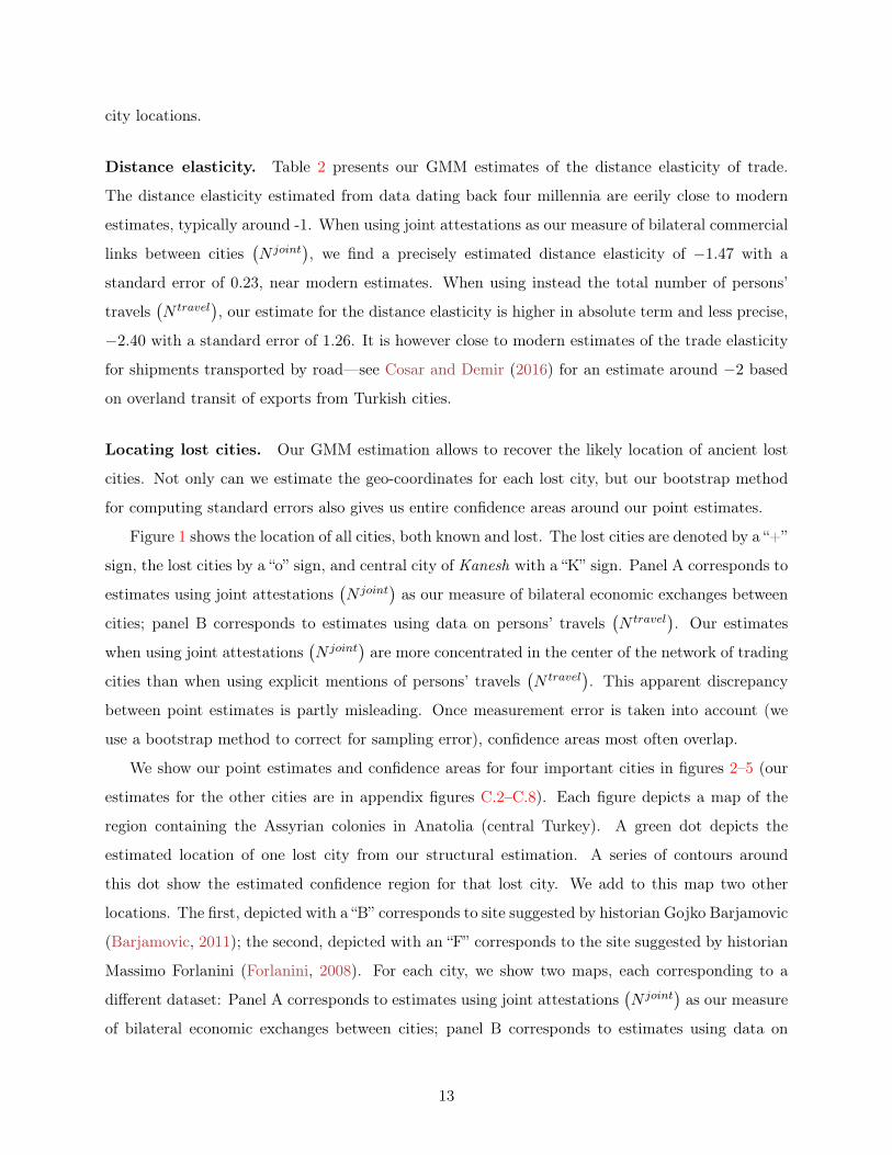
Distance elasticity. Table 2 presents our GMM estimates of the distance elasticity of trade.

The distance elasticity estimated from data dating back four millennia are eerily close to modern

estimates, typically around -1. When using joint attestations as our measure of bilateral commercial

links between cities(N joint

), we find a precisely estimated distance elasticity of −1.47 with a

standard error of 0.23, near modern estimates. When using instead the total number of persons’

travels(N travel

), our estimate for the distance elasticity is higher in absolute term and less precise,

−2.40 with a standard error of 1.26. It is however close to modern estimates of the trade elasticity

for shipments transported by road—see Cosar and Demir (2016) for an estimate around −2 based

on overland transit of exports from Turkish cities.

Locating lost cities. Our GMM estimation allows to recover the likely location of ancient lost

cities. Not only can we estimate the geo-coordinates for each lost city, but our bootstrap method

for computing standard errors also gives us entire confidence areas around our point estimates.

Figure 1 shows the location of all cities, both known and lost. The lost cities are denoted by a “+”

sign, the lost cities by a “o” sign, and central city of Kanesh with a “K” sign. Panel A corresponds to

estimates using joint attestations(N joint

)as our measure of bilateral economic exchanges between

cities; panel B corresponds to estimates using data on persons’ travels(N travel

). Our estimates

when using joint attestations(N joint

)are more concentrated in the center of the network of trading

cities than when using explicit mentions of persons’ travels(N travel

). This apparent discrepancy

between point estimates is partly misleading. Once measurement error is taken into account (we

use a bootstrap method to correct for sampling error), confidence areas most often overlap.

We show our point estimates and confidence areas for four important cities in figures 2–5 (our

estimates for the other cities are in appendix figures C.2–C.8). Each figure depicts a map of the

region containing the Assyrian colonies in Anatolia (central Turkey). A green dot depicts the

estimated location of one lost city from our structural estimation. A series of contours around

this dot show the estimated confidence region for that lost city. We add to this map two other

locations. The first, depicted with a “B” corresponds to site suggested by historian Gojko Barjamovic

(Barjamovic, 2011); the second, depicted with an “F” corresponds to the site suggested by historian

Massimo Forlanini (Forlanini, 2008). For each city, we show two maps, each corresponding to a

different dataset: Panel A corresponds to estimates using joint attestations(N joint

)as our measure

of bilateral economic exchanges between cities; panel B corresponds to estimates using data on

13

persons’ travels(N travel

).

Those maps visually deliver several messages. First, the size and shape of the confidence regions

around our location estimates give a visual sense of the precision of those estimated locations.

For most cities, our estimates are tight, in the sense that the confidence area is at most 100km

wide (to be compared to distances within our network of trading cities of more than a thousand

kms). Second, we can compare our estimated results from two datasets, collected with intrinsically

different methods: joint attestations(N joint

)come from a purely automated string search, while

persons’ travels(N travel

)come from a careful reading and understanding of ancient texts. For all

precisely estimated city locations, the estimates from both datasets are surprisingly close. Third, we

can compare our estimates, obtained by a purely quantitative method—a structural gravity GMM

estimation, to those obtained by historians from a purely qualitative method—reading through texts

and isolating contextual information about likely sites. In several cases where historians’ conjectures

do not drastically diverge, our GMM estimates are very close to these conjectures, giving credence

to both our quantitative method and their qualitative approach. In some cases, our estimates are

close to one historian’s conjecture but not the other’s, giving a strong endorsement to the former.

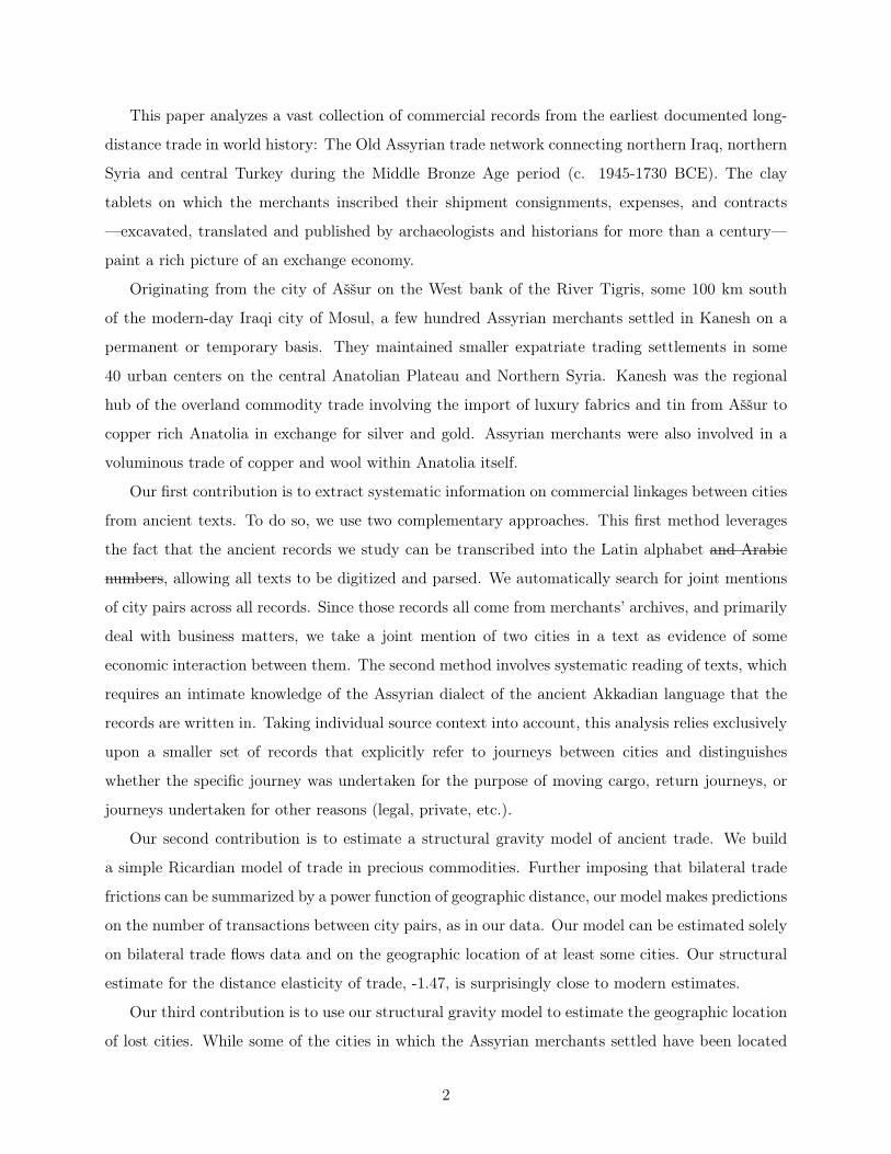
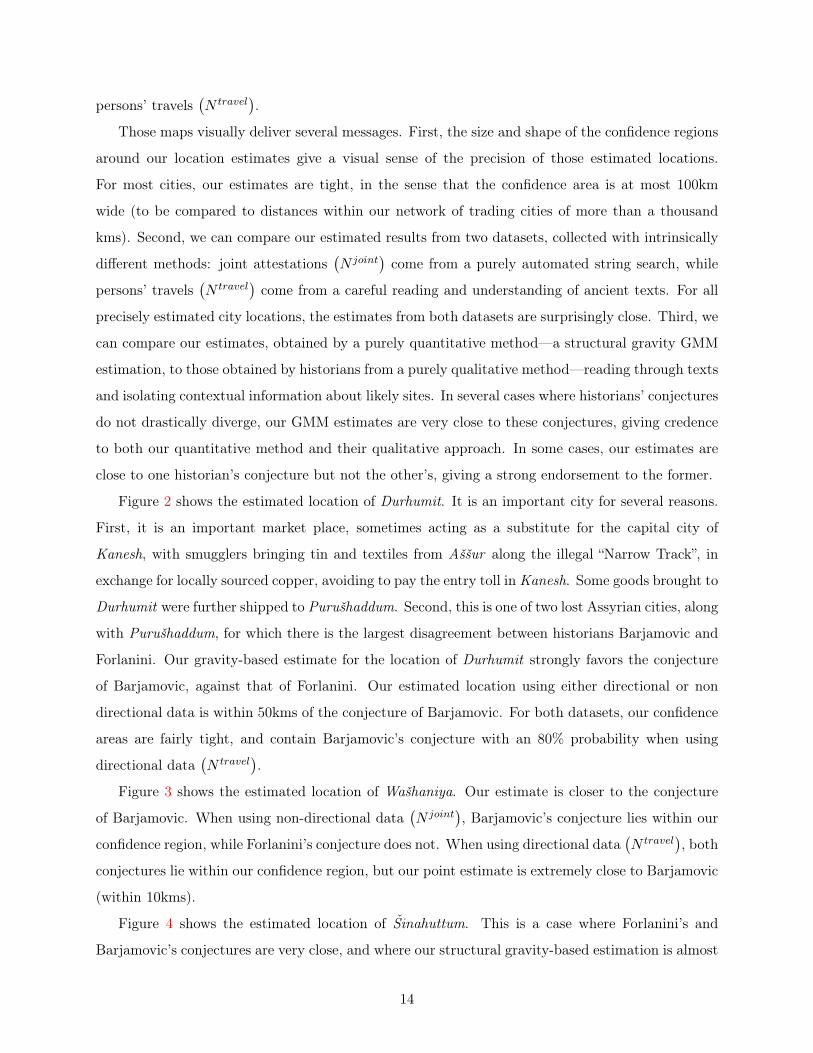
Figure 2 shows the estimated location of Durhumit. It is an important city for several reasons.

First, it is an important market place, sometimes acting as a substitute for the capital city of

Kanesh, with smugglers bringing tin and textiles from Aššur along the illegal “Narrow Track”, in

exchange for locally sourced copper, avoiding to pay the entry toll in Kanesh. Some goods brought to

Durhumit were further shipped to Purušhaddum. Second, this is one of two lost Assyrian cities, along

with Purušhaddum, for which there is the largest disagreement between historians Barjamovic and

Forlanini. Our gravity-based estimate for the location of Durhumit strongly favors the conjecture

of Barjamovic, against that of Forlanini. Our estimated location using either directional or non

directional data is within 50kms of the conjecture of Barjamovic. For both datasets, our confidence

areas are fairly tight, and contain Barjamovic’s conjecture with an 80% probability when using

directional data(N travel

).

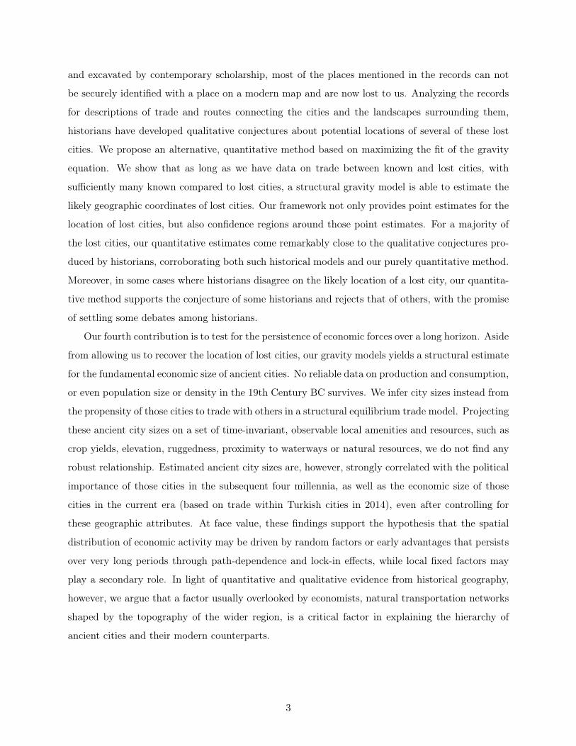
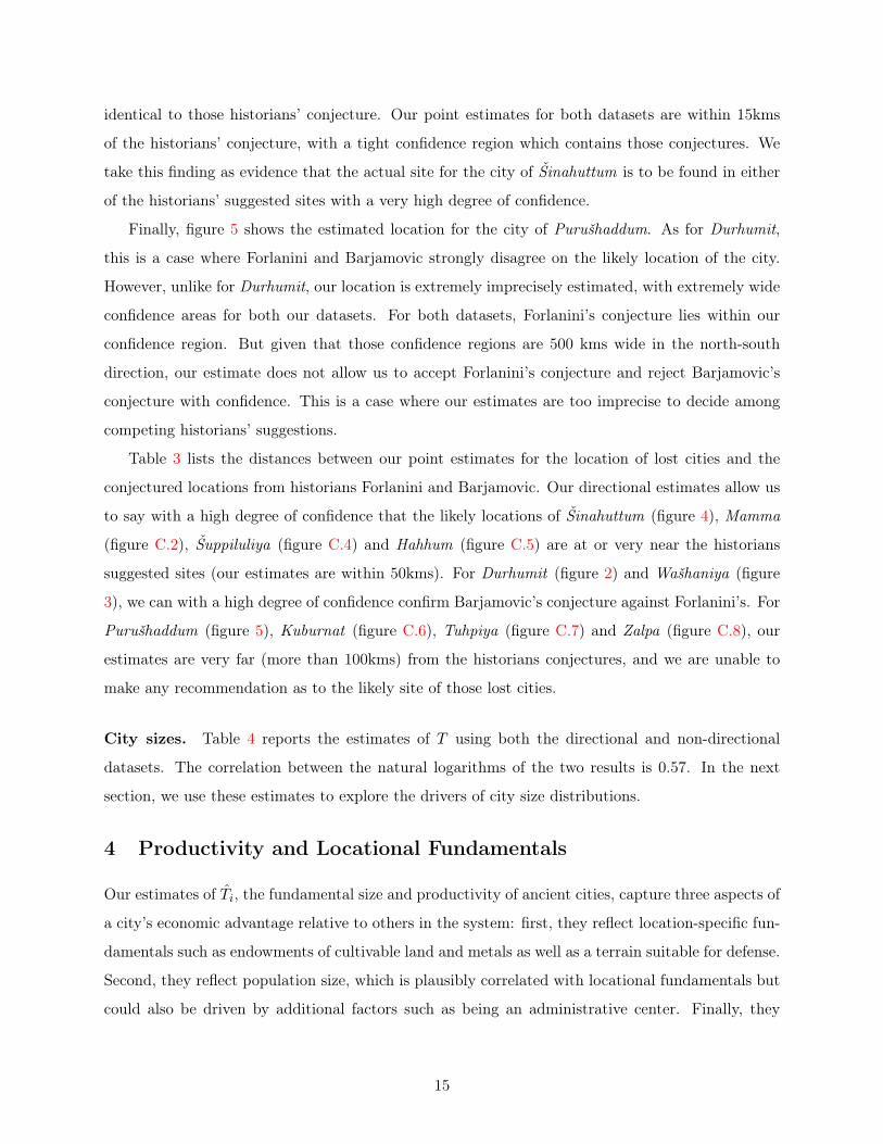
Figure 3 shows the estimated location of Wašhaniya. Our estimate is closer to the conjecture

of Barjamovic. When using non-directional data(N joint

), Barjamovic’s conjecture lies within our

confidence region, while Forlanini’s conjecture does not. When using directional data(N travel

), both

conjectures lie within our confidence region, but our point estimate is extremely close to Barjamovic

(within 10kms).

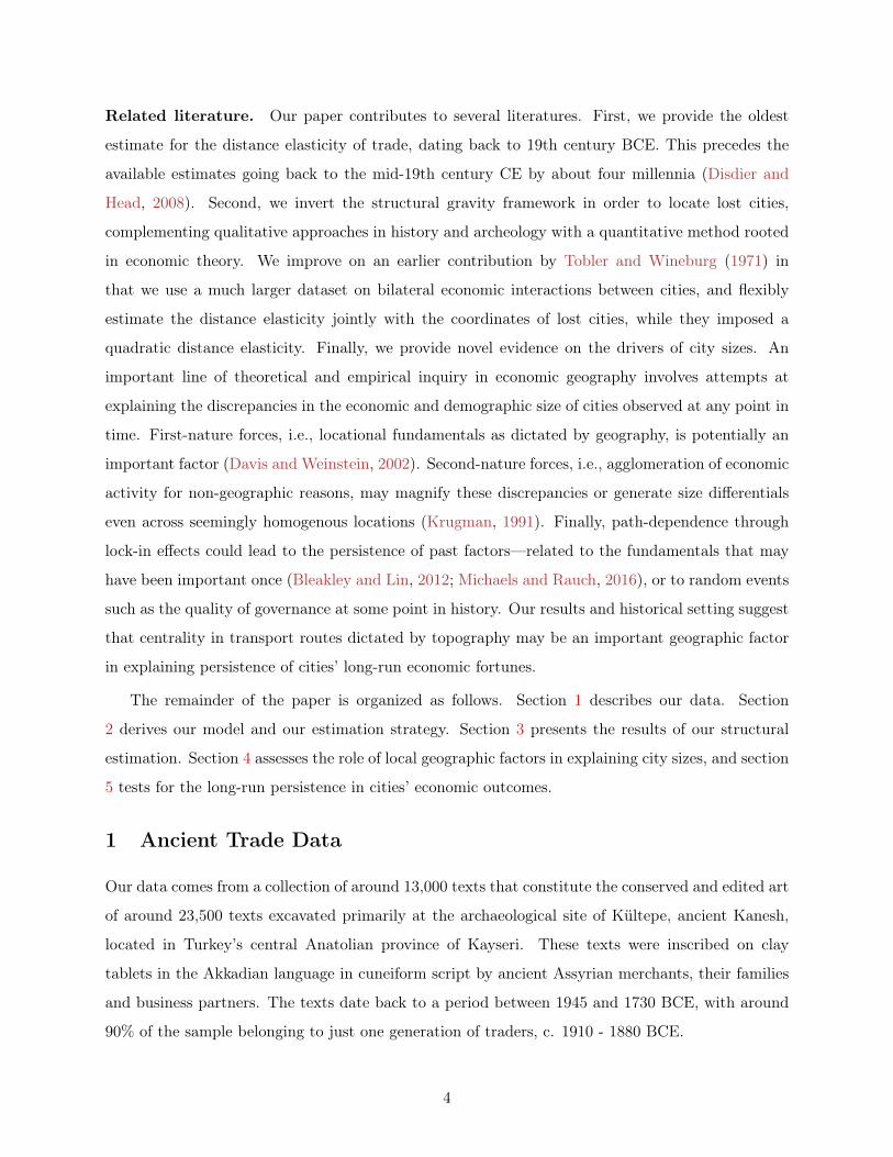
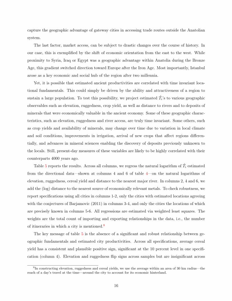
Figure 4 shows the estimated location of Šinahuttum. This is a case where Forlanini’s and

Barjamovic’s conjectures are very close, and where our structural gravity-based estimation is almost

14

identical to those historians’ conjecture. Our point estimates for both datasets are within 15kms

of the historians’ conjecture, with a tight confidence region which contains those conjectures. We

take this finding as evidence that the actual site for the city of Šinahuttum is to be found in either

of the historians’ suggested sites with a very high degree of confidence.

Finally, figure 5 shows the estimated location for the city of Purušhaddum. As for Durhumit,

this is a case where Forlanini and Barjamovic strongly disagree on the likely location of the city.

However, unlike for Durhumit, our location is extremely imprecisely estimated, with extremely wide

confidence areas for both our datasets. For both datasets, Forlanini’s conjecture lies within our

confidence region. But given that those confidence regions are 500 kms wide in the north-south

direction, our estimate does not allow us to accept Forlanini’s conjecture and reject Barjamovic’s

conjecture with confidence. This is a case where our estimates are too imprecise to decide among

competing historians’ suggestions.

Table 3 lists the distances between our point estimates for the location of lost cities and the

conjectured locations from historians Forlanini and Barjamovic. Our directional estimates allow us

to say with a high degree of confidence that the likely locations of Šinahuttum (figure 4), Mamma

(figure C.2), Šuppiluliya (figure C.4) and Hahhum (figure C.5) are at or very near the historians

suggested sites (our estimates are within 50kms). For Durhumit (figure 2) and Wašhaniya (figure

3), we can with a high degree of confidence confirm Barjamovic’s conjecture against Forlanini’s. For

Purušhaddum (figure 5), Kuburnat (figure C.6), Tuhpiya (figure C.7) and Zalpa (figure C.8), our

estimates are very far (more than 100kms) from the historians conjectures, and we are unable to

make any recommendation as to the likely site of those lost cities.

City sizes. Table 4 reports the estimates of T using both the directional and non-directional

datasets. The correlation between the natural logarithms of the two results is 0.57. In the next

section, we use these estimates to explore the drivers of city size distributions.

4 Productivity and Locational Fundamentals

Our estimates of Ti, the fundamental size and productivity of ancient cities, capture three aspects of

a city’s economic advantage relative to others in the system: first, they reflect location-specific fun-

damentals such as endowments of cultivable land and metals as well as a terrain suitable for defense.

Second, they reflect population size, which is plausibly correlated with locational fundamentals but

could also be driven by additional factors such as being an administrative center. Finally, they

15

capture the geographic advantage of gateway cities in accessing trade routes outside the Anatolian

system.

The last factor, market access, can be subject to drastic changes over the course of history. In

our case, this is exemplified by the shift of economic orientation from the east to the west. While

proximity to Syria, Iraq or Egypt was a geographic advantage within Anatolia during the Bronze

Age, this gradient switched direction toward Europe after the Iron Age. Most importantly, Istanbul

arose as a key economic and social hub of the region after two millennia.

Yet, it is possible that estimated ancient productivities are correlated with time invariant loca-

tional fundamentals. This could simply be driven by the ability and attractiveness of a region to

sustain a large population. To test this possibility, we project estimated Ti’s to various geographic

observables such as elevation, ruggedness, crop yield, as well as distance to rivers and to deposits of

minerals that were economically valuable in the ancient economy. Some of these geographic charac-

teristics, such as elevation, ruggedness and river access, are truly time invariant. Some others, such

as crop yields and availability of minerals, may change over time due to variation in local climate

and soil conditions, improvements in irrigation, arrival of new crops that affect regions differen-

tially, and advances in mineral sciences enabling the discovery of deposits previously unknown to

the locals. Still, present-day measures of these variables are likely to be highly correlated with their

counterparts 4000 years ago.

Table 5 reports the results. Across all columns, we regress the natural logarithm of Ti estimated

from the directional data—shown at columns 4 and 6 of table 4—on the natural logarithms of

elevation, ruggedness, cereal yield and distance to the nearest major river. In columns 2, 4 and 6, we

add the (log) distance to the nearest source of economically relevant metals. To check robustness, we

report specifications using all cities in columns 1-2, only the cities with estimated locations agreeing

with the conjectures of Barjamovic (2011) in columns 3-4, and only the cities the locations of which

are precisely known in columns 5-6. All regressions are estimated via weighted least squares. The

weights are the total count of importing and exporting relationships in the data, i.e., the number

of itineraries in which a city is mentioned.8

The key message of table 5 is the absence of a significant and robust relationship between ge-

ographic fundamentals and estimated city productivities. Across all specifications, average cereal

yield has a consistent and plausible positive sign, significant at the 10 percent level in one specifi-

cation (column 4). Elevation and ruggedness flip signs across samples but are insignificant across

8In constructing elevation, ruggedness and cereal yields, we use the average within an area of 30 km radius—thereach of a day’s travel at the time—around the city to account for its economic hinterland.

16

all columns. City productivities are positively correlated with distance to the nearest river, but

the coefficient is significant at the 10 percent level only if we restrict the sample to known cities

(columns 5-6). The counter-intuitive result that proximity to a river does not confer an advantage

to a city is consistent with the fact that due to the steep rapids caused by topography, rivers in

central Anatolia are not suitable for transportation.

We also don’t find any meaningful association between city productivities and distance to copper,

gold or silver deposits. This result, however, should be interpreted with care: among the explanatory

variables, location of metal deposits as currently known is plausibly the least informative one for

the ancient conditions.9

5 Persistence of Economic Outcomes

Next, we test whether ancient prominence persists into the future. The fact that we found no

robust relationship between ancient productivities and geographic attributes in section 4 makes

this exercise informative about the potential role of time-invariant fundamental advantages versus

path-dependence in accounting for long-term economic outcomes of cities and regions.

In what follows, we use all the cities in our sample and weight observations by the total count of

cities’ appearances in the itinerary data. The results are robust to dropping unknown cities if their

locations are estimated to be inconsistent with qualitative evidence, and using known cities only.

5.1 Future Capital Cities

Six cities in our data served as capitals of a state at some point in their history after the era under

study—see Appendix A.1 for detailed information including the list of cities. To check whether

these cities differ from the rest, we first note that average ln(Ti) equals 7.45 and 5.67 for capital

and non-capital cities, respectively. Similarly, median productivity among capital cities is 1.45 log

points higher than among non-capital cities.

For a more detailed analysis, we regress a binary variable that takes the value one for capitals,

and zero otherwise, on ln(Ti) while controlling for the set of geographic attributes introduced above.

Table 6 reports the results. The first two columns are results from a linear probability model. The

third column reports average marginal effects from a probit regression. Across all columns, ancient

productivity estimates are positively correlated with the future capital status of cities with varying

degrees of significance while geographic attributes are estimated to be insignificant.

9In fact, the minimum distance is above 30 km for all three metals.

17

The result that productivity in the past is positively correlated with the propensity of a city

being a capital in the future could be driven by various channels that are not necessarily mutually

exclusive: it could be that a city’s prominence persists and increases its probability of being selected

as the center of a state that takes the region under its control. Similarly, such cities may simply

have a higher chance of surviving into the future. Alternatively, their resource base and prominence

could support a military and political expansion, as a result of which they become the center of a

state commanding a wider territory. This latter possibility, however, is not supported by the result

that the resource-based geographic fundamentals used as controls are insignificant.

5.2 Present-day Productivity Estimates

Moving further into the future, we now ask whether ancient productivities are correlated with

present-day productivity estimates of the same locations. To address this question, we find the set

of present-day cities in Turkey corresponding to our system of ancient cities. There are 14 such cities

since some contain multiple ancient cities within their boundary. Using 2014 trade flows within this

system of 14 cities, we estimate Tmoderni by the same econometric procedure except that we do not

need to estimate locations in this case.10 Denoting the original estimates of ancient productivities

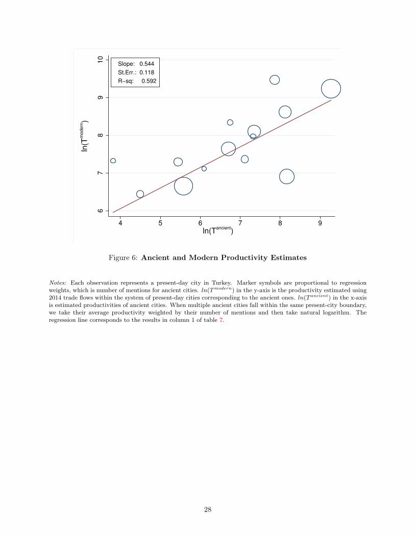
by T ancienti , figure 6 and table 7 present the results. Despite being estimated using trade flows

that are 4000 years apart, the correlation is remarkably high and significant. Ancient productivities

capture around 60 percent of the variation in modern productivities.

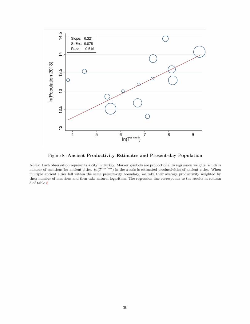
5.3 Present-day GDP and Population

Continuing the same line of inquiry, we replace the dependent variable with the (log) total in-

come and population of present-day cities. Since the Turkish Statistical Institute does not publish

city-level GDP data for the period after 2001, we use estimates by the Economic Policy Research

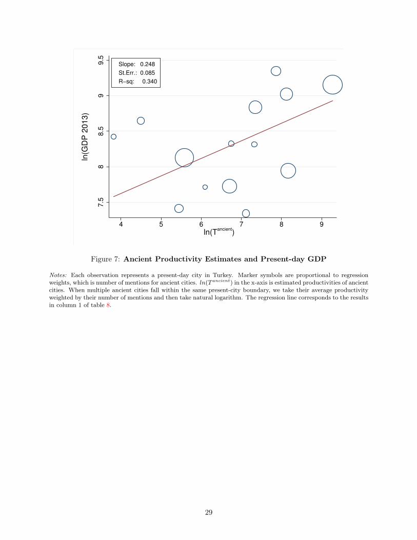
Foundation for 2013, the latest year for which data available.11 Figures 7 and 8, and table 8 report

the results, which are consistent with subsection 5.2. Even after controlling for time invariant geo-

graphic attributes, productivity estimated from ancient data is correlated with present-day income

and population.12

10The only ancient city that is not within the boundaries of present-day Turkey is Qattara, which is near TalAfar/Iraq. Since 2014 trade data is only for Turkish cities, this ancient city drops from the subsequent analysis.

11The data is accessible at the website http://www.tepav.org.tr/tr/haberler/s/4054. Economic Policy Re-search Foundation uses nighttime luminosity to estimate city-level incomes as in Hodler and Raschky (2014).

12Figures 6,7 and 8 leave out Ankara, which is an outlier with high present-day levels due to its status as Turkey’scapital city.

18

5.4 Discussion

Our exploration yields an intriguing result: a variety of geographic attributes—agricultural poten-

tial, access to mineral resources, distance to rivers and terrain-related defensive capability—are not

correlated with estimated economic size of ancient cities, which are in turn correlated with future

prominence and economic size of the same localities. We now discuss whether this strong persistence

in regional outcomes lends support to models of city growth through path-dependence and lock-in

effects, as convincingly demonstrated by Bleakley and Lin (2012) for the case of mid-Atlantic and

southern U.S. cities that were once portage sites at fall lines, and by Michaels and Rauch (2016) for

French cities originating from Roman towns.

A potential caveat is that the geographic attributes we used in our analysis do not adequately

capture locational advantages that matter throughout history in a persistent manner. One such

factor is the geography of natural transport networks. In a rich account of historical geography

of Anatolia, Ramsay (1890) argues that the topography of the region imposes strict restrictions

on main passages in the east-west and north-south directions. As a result, cities located on these

routes—especially those at the intersection points, the so-called road-knots—enjoyed an advantage

of being ideal distribution centers for regional trade.13 While we do not have a readily available

quantitative measure of this geographic attribute, we reckon that it plays an important role in

explaining the long-run persistence of economic size across Anatolian cities. The very location of

Kanesh and the present-day city of Kayseri—whose center is only 20 km away from Kanesh—is

a case in point: it lies at the western side of Taurus crossings connecting the central Anatolia

plateau to the upper Mesopotamian plain. Several other ancient and corresponding present-day

cities with high productivity estimates, such as Hurama-Elbistan, Zalpa-Gaziantep, Salatuwar-

Eskisehir and Samuha-Sivas, are also placed on road-knots (Barjamovic, 2011; French, 1993). The

main transportation arteries in Turkey overlap with the known Roman roads, which themselves

may have presumably followed the ancient routes from the Bronze Age.14 Recent GIS analysis by

Palmisano (2013) and Palmisano and Altaweel (2015) confirms that ancient routes were indeed very

close to be the least-cost pathways, which increases our confidence that the modern-transportation

routes are not merely overlaid on ancient networks through a lock-in effect.

13A similar analysis by Cronon (2009) emphasizes Chicago’s location at the intersection point of overland andwater transportation routes as a key factor in its growth.

14A similar long-run continuity in the Inca road network has been used by Martincus et al. (2017) to instrumentfor the development of the modern road system in Peru.

19

Conclusion

Business documents dating back to the Bronze Age—inscribed into clay tablets and unearthed from

ancient sites in Anatolia—give us a window to analyze economic interactions between Assyrian

merchants 4000 years ago. The data allows us to construct proxies for trade between ancient cities

and estimate a structural gravity model.

Three main results emerge. First, the estimated distance elasticity of trade is remarkably close to

estimates from present-day datasets. This is consistent with Disdier and Head (2008) who document

a puzzling persistence of the distance effect in international trade during the modern-era. In light

of the apparent improvements in transportation technologies, recent theories offer explanations for

this pattern based on trade barriers that are very persistent themselves, such as the way traders

form networks and interact within them (Chaney, 2014). The ancient setting under study is one

in which such relationships are of primary importance to conduct long-distance trade under severe

enforcement problems. In future work, we hope to utilize the information on individual merchants

and their networks available in the ancient data to shed further light on this subject.

Second, more cities are named in ancient texts than can be located unambiguously by arche-

ological evidence. Assyriologists develop conjectures on potential sites based on qualitative and

linguistic evidence (Barjamovic, 2011). In a rare form of collaboration across disciplines, we use a

theory-based quantitative method from economics to inform this quest in the field of history. The

structural gravity model delivers estimates for the coordinates of the lost cities. For a majority

of cases, our quantitative estimates are remarkably close to qualitative conjectures from several

historians. In some cases where historians disagree on the likely site of lost cities, our quantitative

method supports the conjecture of some historians and rejects that of others, with the promise of

settling some debates among historians.

Finally, we analyze the correlation between the estimated economic size and observable time-

invariant geographic attributes of ancient cities, as well as their future economic outcomes. This

exercise brings fresh evidence on a seminal question in economic geography: what explains the size

of cities? We do not find any significant explanatory power for ancient economic size in agricultural

potential, mineral resources and terrain-related defensive capability. We do, however, find that

ancient economic size predicts the propensity of these cities to become a regional center in the

future, as well as the income and population of corresponding regions in present-day Turkey. We

argue that the persistence of cities’ fortunes across 4000 years can best be explained by their time-

invariant locational advantage in the topography of trade routes, as proposed by Ramsay (1890).

20

References

Anderson, J. E. and E. van Wincoop (2003): “Gravity with Gravitas: A Solution to the BorderPuzzle,” American Economic Review, 93, 170–92.

Barjamovic, G. (2011): A Historical Geography of Anatolia in the Old Assyrian Colony Period,Museum Tusculanum Press.

Bleakley, H. and J. Lin (2012): “Portage and path dependence,” The quarterly journal ofeconomics, qjs011.

Chaney, T. (2014): “The network structure of international trade,” The American EconomicReview, 104, 3600–3634.

Cosar, A. K. and B. Demir (2016): “Domestic road infrastructure and international trade:Evidence from Turkey,” Journal of Development Economics, 118, 232 – 244.

Cronon, W. (2009): Nature’s metropolis: Chicago and the Great West, WW Norton &amp; Com-pany.

Davis, D. R. and D. E. Weinstein (2002): “Bones, bombs, and break points: the geography ofeconomic activity,” American Economic Review, 1269–1289.

Disdier, A.-C. and K. Head (2008): “The puzzling persistence of the distance effect on bilateraltrade,” The Review of Economics and statistics, 90, 37–48.

Eaton, J. and S. Kortum (2002): “Technology, Geography and Trade,” Econometrica, 70, 1741–79.

Eaton, J., S. Kortum, and S. Sotelo (2012): “International Trade: Linking Micro and Macro,”NBER Working Paper No.17864.

Forlanini, M. (2008): “The Central Provinces of Hatti. An Updating,” in New Perspectives onthe Historical Geography and Topography of Anatolia in the II and I Millennium BC, ed. byK. Strobel, LoGisma Editore, 1, 145–188.

French, D. (1993): “Colonia Archelais and Road-Knots,” Aspects of Art and Iconography: Anatoliaand Its Neighbors Studies in Honor of Nimet Özgüç, 201–7.

Hodler, R. and P. A. Raschky (2014): “Regional Favoritism,” The Quarterly Journal of Eco-nomics.

Kortum, S. S. (1997): “Research, patenting, and technological change,” Econometrica, 65, 1389–1419.

Krugman, P. (1980): “Scale Economies, Product Differentiation, and the Patterns of Trade,”American Economic Review, 70, 950–59.

——— (1991): “Increasing returns and economic geography,” Journal of political economy, 99, 483–499.

Martincus, C. V., J. Carballo, and A. Cusolito (2017): “Roads, exports and employment:Evidence from a developing country,” Journal of Development Economics, 125, 21–39.

21

Michaels, G. and F. Rauch (2016): “Resetting the Urban Network: 117-2012,” The EconomicJournal.

Palmisano, A. (2013): “Computational and Spatial Approaches to the Commercial Landscapesand Political Geography of the Old Assyrian Colony Period.” in Time and History in the AncientNear East. Proceedings of the 56th Rencontre Assyriologique Internationale, Barcelona, July 26-30, 2010., Eisenbrauns., 767–783.

Palmisano, A. and M. Altaweel (2015): “Landscapes of interaction and conflict in the MiddleBronze Age: From the open plain of the Khabur Triangle to the mountainous inland of CentralAnatolia,” Journal of Archaeological Science: Reports, 3, 216–236.

Ramsay, W. M. (1890): The historical geography of Asia Minor, vol. 4, John Murray.

Silva, J. S. and S. Tenreyro (2006): “The log of gravity,” The Review of Economics andstatistics, 88, 641–658.

Tobler, W. and S. Wineburg (1971): “A Cappadocian speculation,” Nature, 231, 39–41.

22

Figures

Panel A: Non-directional trade (N jointij )

Panel B: Directional trade (N travelij )

Figure 1: Known and lost cities.

Notes: The maps show the of all Assyrian cities. The “+” signs correspond to the location of known cities. The “K”sign denotes Kanesh, the capital city of Assyrian colonies. The “o” signs denote the estimated location of lost cities,from the GMM estimation in (7). Panel A presents the estimates using non-directional data from joint attestationsof city names

(N jointij

). Panel B presents the estimates using directional data on persons’ travels

(N travelij

). Sources:

Old Assyrian Text Project.

23

Panel A: Non-directional trade (N jointij )

Panel B: Directional trade (N travelij )

Figure 2: Finding lost cities: Durhumit.

Notes: The maps show the estimated location for the ancient city of Durhumit . In both maps, the location denotedby “B” corresponds to the site suggested by historian Gojko Barjamovic (Barjamovic, 2011), and the location denotedby “F” to the site suggested by historian Massimo Forlanini (Forlanini, 2008). Both historians base their suggestionon qualitative information collected from historical records, in particular the topography of the site, and references tolandmarks identified in more recent historical texts. The green dot correspond to the estimated location from solvinga structural gravity model, the GMM estimation in (7). Panel A presents the estimates using non-directional datafrom joint attestations of city names

(N jointij

). Panel B presents the estimates using directional data on persons’

travels(N travelij

). The contours around the green dot are a contour plot of the confidence area drawn from 83 out

of 100 bootstrapped trials (panel A) and 65 out of 100 bootstrapped trials (panel B). Sources: Old Assyrian TextProject.

24

Panel A: Non-directional trade (N jointij )

Panel B: Directional trade (N travelij )

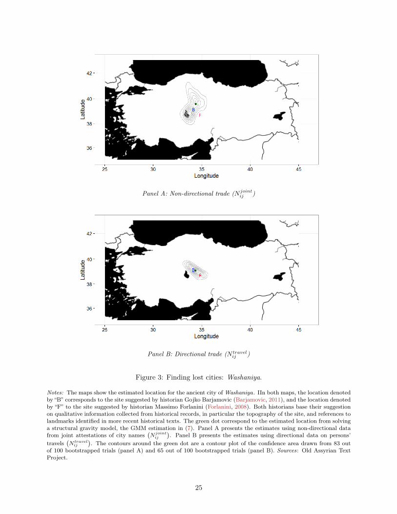
Figure 3: Finding lost cities: Washaniya.

Notes: The maps show the estimated location for the ancient city of Washaniya. IIn both maps, the location denotedby “B” corresponds to the site suggested by historian Gojko Barjamovic (Barjamovic, 2011), and the location denotedby “F” to the site suggested by historian Massimo Forlanini (Forlanini, 2008). Both historians base their suggestionon qualitative information collected from historical records, in particular the topography of the site, and references tolandmarks identified in more recent historical texts. The green dot correspond to the estimated location from solvinga structural gravity model, the GMM estimation in (7). Panel A presents the estimates using non-directional datafrom joint attestations of city names

(N jointij

). Panel B presents the estimates using directional data on persons’

travels(N travelij

). The contours around the green dot are a contour plot of the confidence area drawn from 83 out

of 100 bootstrapped trials (panel A) and 65 out of 100 bootstrapped trials (panel B). Sources: Old Assyrian TextProject.

25

Panel A: Non-directional trade (N jointij )

Panel B: Directional trade (N travelij )

Figure 4: Finding lost cities: Sinahuttum.

Notes: The maps show the estimated location for the ancient city of Sinahuttum. In both maps, the location denotedby “B” corresponds to the site suggested by historian Gojko Barjamovic (Barjamovic, 2011), and the location denotedby “F” to the site suggested by historian Massimo Forlanini (Forlanini, 2008). Both historians base their suggestionon qualitative information collected from historical records, in particular the topography of the site, and references tolandmarks identified in more recent historical texts. The green dot correspond to the estimated location from solvinga structural gravity model, the GMM estimation in (7). Panel A presents the estimates using non-directional datafrom joint attestations of city names

(N jointij

). Panel B presents the estimates using directional data on persons’

travels(N travelij

). The contours around the green dot are a contour plot of the confidence area drawn from 83 out

of 100 bootstrapped trials (panel A) and 65 out of 100 bootstrapped trials (panel B). Sources: Old Assyrian TextProject.

26

Panel A: Non-directional trade (N jointij )

Panel B: Directional trade (N travelij )

Figure 5: Finding lost cities: Purushaddum.

Notes: The maps show the estimated location for the ancient city of Purushaddum. In both maps, the location denotedby “B” corresponds to the site suggested by historian Gojko Barjamovic (Barjamovic, 2011), and the location denotedby “F” to the site suggested by historian Massimo Forlanini (Forlanini, 2008). Both historians base their suggestionon qualitative information collected from historical records, in particular the topography of the site, and references tolandmarks identified in more recent historical texts. The green dot correspond to the estimated location from solvinga structural gravity model, the GMM estimation in (7). Panel A presents the estimates using non-directional datafrom joint attestations of city names

(N jointij

). Panel B presents the estimates using directional data on persons’

travels(N travelij

). The contours around the green dot are a contour plot of the confidence area drawn from 83 out

of 100 bootstrapped trials (panel A) and 65 out of 100 bootstrapped trials (panel B). Sources: Old Assyrian TextProject.

27

67

89

10

ln(T

mo

de

rn)

4 5 6 7 8 9

ln(Tancient

)

Slope: 0.544

St.Err.: 0.118

R−sq: 0.592

Figure 6: Ancient and Modern Productivity Estimates

Notes: Each observation represents a present-day city in Turkey. Marker symbols are proportional to regressionweights, which is number of mentions for ancient cities. ln(Tmodern) in the y-axis is the productivity estimated using2014 trade flows within the system of present-day cities corresponding to the ancient ones. ln(T ancient) in the x-axisis estimated productivities of ancient cities. When multiple ancient cities fall within the same present-city boundary,we take their average productivity weighted by their number of mentions and then take natural logarithm. Theregression line corresponds to the results in column 1 of table 7.

28

7.5

88

.59

9.5

ln(G

DP

2013)

4 5 6 7 8 9

ln(Tancient

)

Slope: 0.248

St.Err.: 0.085

R−sq: 0.340

Figure 7: Ancient Productivity Estimates and Present-day GDP

Notes: Each observation represents a present-day city in Turkey. Marker symbols are proportional to regressionweights, which is number of mentions for ancient cities. ln(T ancient) in the x-axis is estimated productivities of ancientcities. When multiple ancient cities fall within the same present-city boundary, we take their average productivityweighted by their number of mentions and then take natural logarithm. The regression line corresponds to the resultsin column 1 of table 8.

29

12

12

.51

31

3.5

14

14

.5

ln(P

opula

tion 2

013)

4 5 6 7 8 9

ln(Tancient

)

Slope: 0.321

St.Err.: 0.078

R−sq: 0.516

Figure 8: Ancient Productivity Estimates and Present-day Population

Notes: Each observation represents a city in Turkey. Marker symbols are proportional to regression weights, which isnumber of mentions for ancient cities. ln(T ancient) in the x-axis is estimated productivities of ancient cities. Whenmultiple ancient cities fall within the same present-city boundary, we take their average productivity weighted bytheir number of mentions and then take natural logarithm. The regression line corresponds to the results in column3 of table 8.

30

Tables

Table 1: Descriptive Statistics

Mean St. Dev. Observations

Directional, human-read dataKnown cities 16Lost cities 11

N cargoij | all 0.49 1.98 650

N cargoij | N > 0 3.24 4.15 98

N travelij | all 0.56 2.17 702

N travelij | N > 0 3.27 4.31 122

Non-directional, machine-read dataKnown cities 17Lost cities 12

N jointij | all 2.32 7.57 406

N jointij | N > 0 5.62 10.97 168

Notes: The ancient data comes from a textual analysis of clay tablets inscribed in the cuneiform alphabet, sent byAssyrian merchants in the 2nd millennium BCE. Most texts are digitized and available through the Old AssyrianText Project.

Table 2: GMM Estimates – Distance Elasticity (ζ)

Non-directional DirectionalData Data(1) (2)

Distance elasticity: ζ 1.47 2.40(0.23) (1.26)

Number of observations 406 702Number of observations 6= 0 168 122Number of trade flows 944 405

Number of starting values 2000 2000Achieved minimum 1.540 4.384

Number of bootstraps (trials) 100 100Number of bootstraps (successes) 83 65

Notes: This table presents the results of the GMM estimates of the distance elasticity of trade (ζ) from (7). Column1 uses non directional data on joint attestations of city names

(N joint

); column 2 uses directional data on persons’

travels(N travel

). Bootstrapped standard errors in parentheses. The lower panel of the table describes key statistics

from the GMM estimation.

31

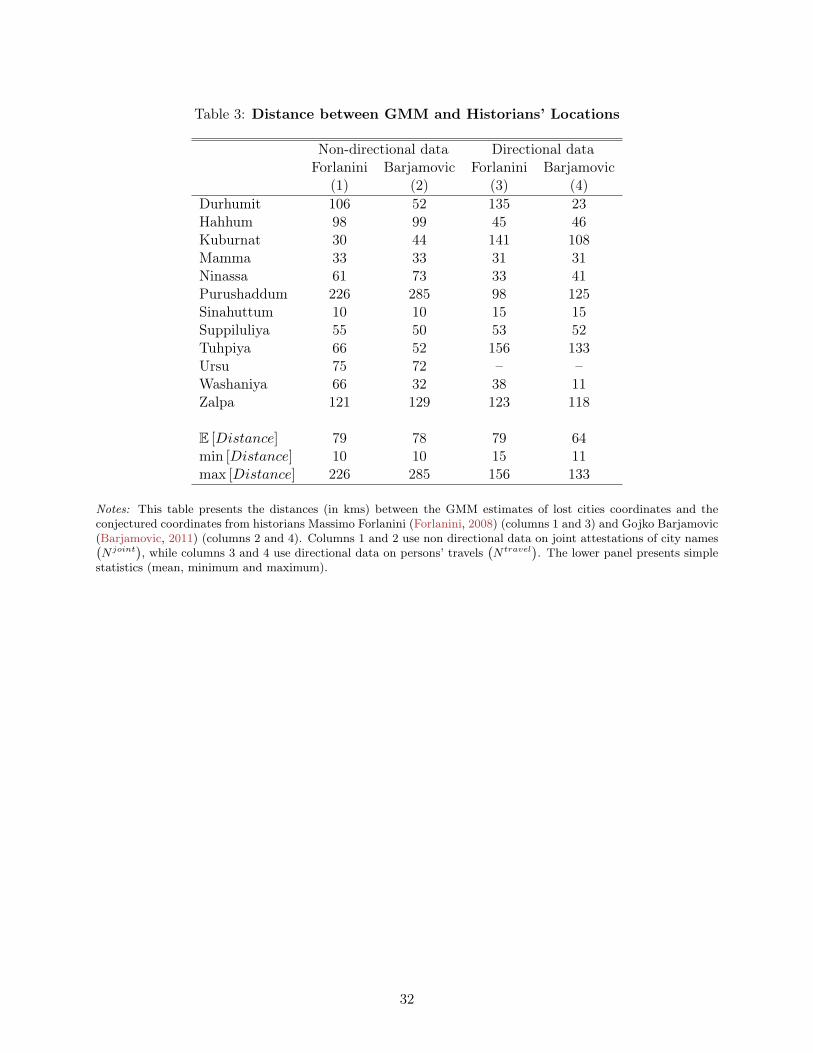
Table 3: Distance between GMM and Historians’ Locations

Non-directional data Directional dataForlanini Barjamovic Forlanini Barjamovic

(1) (2) (3) (4)Durhumit 106 52 135 23Hahhum 98 99 45 46Kuburnat 30 44 141 108Mamma 33 33 31 31Ninassa 61 73 33 41Purushaddum 226 285 98 125Sinahuttum 10 10 15 15Suppiluliya 55 50 53 52Tuhpiya 66 52 156 133Ursu 75 72 – –Washaniya 66 32 38 11Zalpa 121 129 123 118

E [Distance] 79 78 79 64min [Distance] 10 10 15 11max [Distance] 226 285 156 133

Notes: This table presents the distances (in kms) between the GMM estimates of lost cities coordinates and theconjectured coordinates from historians Massimo Forlanini (Forlanini, 2008) (columns 1 and 3) and Gojko Barjamovic(Barjamovic, 2011) (columns 2 and 4). Columns 1 and 2 use non directional data on joint attestations of city names(N joint

), while columns 3 and 4 use directional data on persons’ travels

(N travel

). The lower panel presents simple

statistics (mean, minimum and maximum).

32

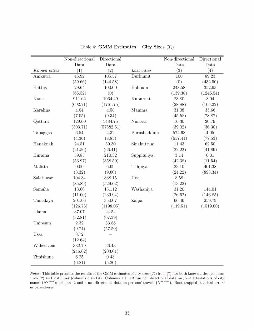
Table 4: GMM Estimates – City Sizes (Ti)

Non-directional Directional Non-directional DirectionalData Data Data Data

Known cities (1) (2) Lost cities (3) (4)Amkuwa 45.92 105.37 Durhumit 100 89.23

(59.66) (144.58) (0) (432.50)Hattus 29.64 100.00 Hahhum 248.58 352.63

(65.52) (0) (139.38) (1246.54)Kanes 911.62 1064.49 Kuburnat 23.80 8.94

(692.71) (1761.75) (28.88) (105.22)Karahna 4.04 4.58 Mamma 31.08 35.66

(7.05) (9.34) (45.58) (73.87)Qattara 129.60 5484.75 Ninassa 16.30 20.79

(303.71) (57582.51) (39.02) (36.30)Tapaggas 6.54 4.32 Purushaddum 574.98 4.05

(4.36) (8.85) (657.41) (77.53)Hanaknak 24.51 50.30 Sinahuttum 11.43 62.50

(21.56) (66.41) (22.22) (41.89)Hurama 59.83 210.32 Suppiluliya 3.14 0.01

(53.97) (358.59) (42.38) (11.54)Malitta 0.00 6.09 Tuhpiya 23.10 401.38

(3.32) (9.00) (24.22) (898.34)Salatuwar 104.34 338.15 Ursu 8.58 –

(85.89) (529.62) (13.22) –Samuha 13.66 151.12 Washaniya 31.20 144.01

(11.00) (239.94) (26.62) (146.85)Timelkiya 201.06 350.07 Zalpa 66.46 259.79

(126.73) (1198.05) (119.51) (1519.60)Ulama 37.07 24.54

(32.81) (67.39)Unipsum 2.32 33.88

(9.74) (57.50)Ussa 8.72 –

(12.64) –Wahsusana 332.79 26.43

(246.62) (203.01)Zimishuna 6.25 0.43

(6.81) (5.20)

Notes: This table presents the results of the GMM estimates of city sizes (Ti) from (7), for both known cities (columns1 and 2) and lost cities (columns 3 and 4). Columns 1 and 3 use non directional data on joint attestations of citynames

(N joint

); columns 2 and 4 use directional data on persons’ travels

(N travel

). Bootstrapped standard errors

in parentheses.

33

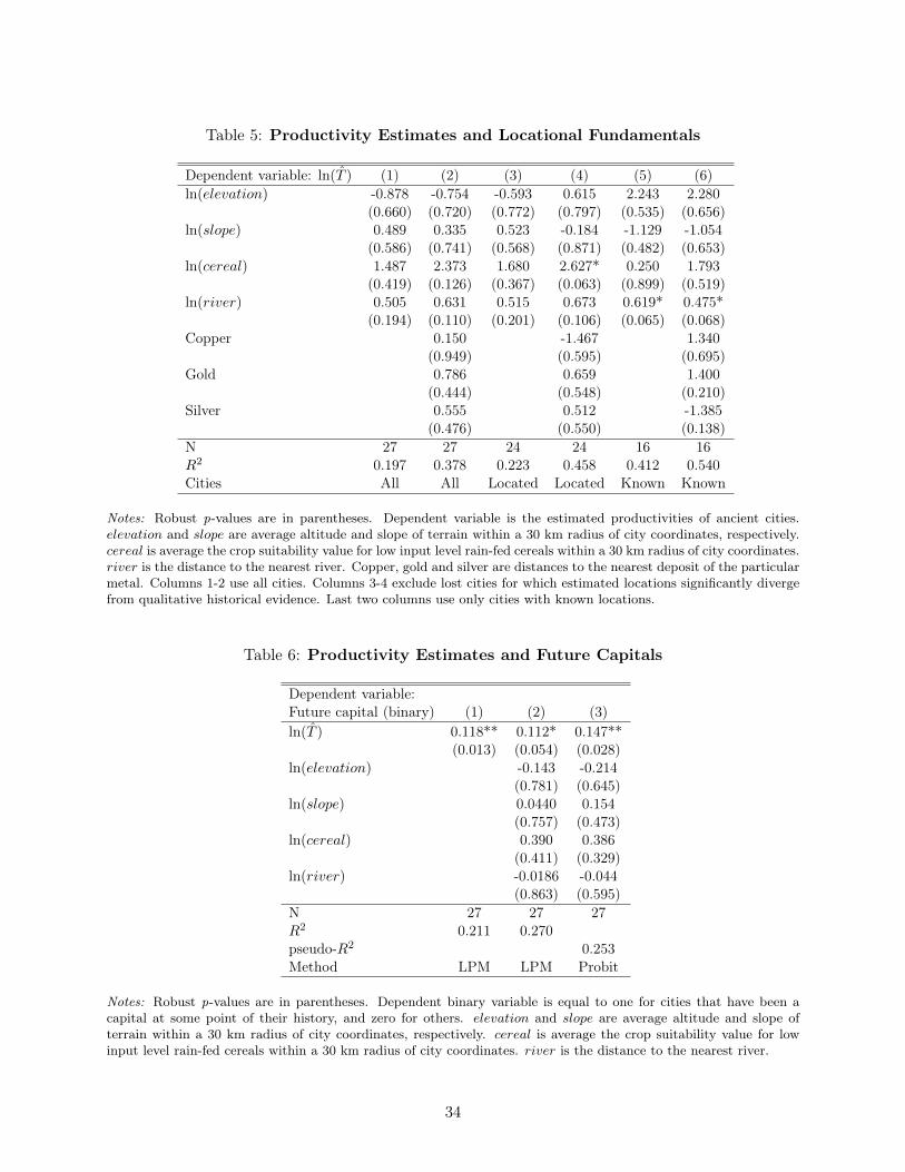
Table 5: Productivity Estimates and Locational Fundamentals

Dependent variable: ln(T ) (1) (2) (3) (4) (5) (6)ln(elevation) -0.878 -0.754 -0.593 0.615 2.243 2.280

(0.660) (0.720) (0.772) (0.797) (0.535) (0.656)ln(slope) 0.489 0.335 0.523 -0.184 -1.129 -1.054

(0.586) (0.741) (0.568) (0.871) (0.482) (0.653)ln(cereal) 1.487 2.373 1.680 2.627* 0.250 1.793

(0.419) (0.126) (0.367) (0.063) (0.899) (0.519)ln(river) 0.505 0.631 0.515 0.673 0.619* 0.475*

(0.194) (0.110) (0.201) (0.106) (0.065) (0.068)Copper 0.150 -1.467 1.340

(0.949) (0.595) (0.695)Gold 0.786 0.659 1.400

(0.444) (0.548) (0.210)Silver 0.555 0.512 -1.385

(0.476) (0.550) (0.138)N 27 27 24 24 16 16R2 0.197 0.378 0.223 0.458 0.412 0.540Cities All All Located Located Known Known

Notes: Robust p-values are in parentheses. Dependent variable is the estimated productivities of ancient cities.elevation and slope are average altitude and slope of terrain within a 30 km radius of city coordinates, respectively.cereal is average the crop suitability value for low input level rain-fed cereals within a 30 km radius of city coordinates.river is the distance to the nearest river. Copper, gold and silver are distances to the nearest deposit of the particularmetal. Columns 1-2 use all cities. Columns 3-4 exclude lost cities for which estimated locations significantly divergefrom qualitative historical evidence. Last two columns use only cities with known locations.

Table 6: Productivity Estimates and Future Capitals

Dependent variable:Future capital (binary) (1) (2) (3)ln(T ) 0.118** 0.112* 0.147**

(0.013) (0.054) (0.028)ln(elevation) -0.143 -0.214

(0.781) (0.645)ln(slope) 0.0440 0.154

(0.757) (0.473)ln(cereal) 0.390 0.386

(0.411) (0.329)ln(river) -0.0186 -0.044

(0.863) (0.595)N 27 27 27R2 0.211 0.270pseudo-R2 0.253Method LPM LPM Probit

Notes: Robust p-values are in parentheses. Dependent binary variable is equal to one for cities that have been acapital at some point of their history, and zero for others. elevation and slope are average altitude and slope ofterrain within a 30 km radius of city coordinates, respectively. cereal is average the crop suitability value for lowinput level rain-fed cereals within a 30 km radius of city coordinates. river is the distance to the nearest river.

34

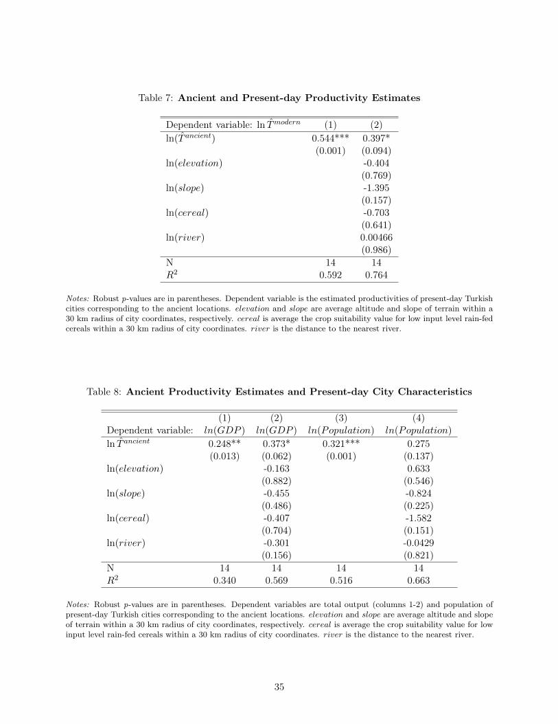
Table 7: Ancient and Present-day Productivity Estimates

Dependent variable: ln Tmodern (1) (2)ln(T ancient) 0.544*** 0.397*

(0.001) (0.094)ln(elevation) -0.404

(0.769)ln(slope) -1.395

(0.157)ln(cereal) -0.703

(0.641)ln(river) 0.00466

(0.986)N 14 14R2 0.592 0.764

Notes: Robust p-values are in parentheses. Dependent variable is the estimated productivities of present-day Turkishcities corresponding to the ancient locations. elevation and slope are average altitude and slope of terrain within a30 km radius of city coordinates, respectively. cereal is average the crop suitability value for low input level rain-fedcereals within a 30 km radius of city coordinates. river is the distance to the nearest river.

Table 8: Ancient Productivity Estimates and Present-day City Characteristics

(1) (2) (3) (4)Dependent variable: ln(GDP ) ln(GDP ) ln(Population) ln(Population)

ln T ancient 0.248** 0.373* 0.321*** 0.275(0.013) (0.062) (0.001) (0.137)

ln(elevation) -0.163 0.633(0.882) (0.546)

ln(slope) -0.455 -0.824(0.486) (0.225)

ln(cereal) -0.407 -1.582(0.704) (0.151)

ln(river) -0.301 -0.0429(0.156) (0.821)

N 14 14 14 14R2 0.340 0.569 0.516 0.663

Notes: Robust p-values are in parentheses. Dependent variables are total output (columns 1-2) and population ofpresent-day Turkish cities corresponding to the ancient locations. elevation and slope are average altitude and slopeof terrain within a 30 km radius of city coordinates, respectively. cereal is average the crop suitability value for lowinput level rain-fed cereals within a 30 km radius of city coordinates. river is the distance to the nearest river.

35

Technical Appendix for:Trade, Merchants, and the Lost Cities of the Bronze Age

(not for publication)

by Gojko Barjamovic, Thomas Chaney, Kerem Coşar, and Ali Hortaçsu

A Additional Data

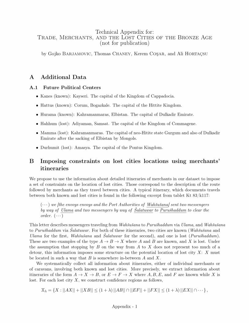
A.1 Future Political Centers

• Kanes (known): Kayseri. The capital of the Kingdom of Cappadocia.

• Hattus (known): Corum, Bogazkale. The capital of the Hittite Kingdom.

• Hurama (known): Kahramanmaras, Elbistan. The capital of Dulkadir Emirate.

• Hahhum (lost): Adiyaman, Samsat. The capital of the Kingdom of Commagene.

• Mamma (lost): Kahramanmaras. The capital of neo-Hitite state Gurgum and also of DulkadirEmirate after the sacking of Elbistan by Mongols.

• Durhumit (lost): Amasya. The capital of the Pontus Kingdom.

B Imposing constraints on lost cities locations using merchants’itineraries

We propose to use the information about detailed itineraries of merchants in our dataset to imposea set of constraints on the location of lost cities. Those correspond to the description of the routefollowed by merchants as they travel between cities. A typical itinerary, which documents travelsbetween both known and lost cities is found in the following excerpt from tablet Kt 83/k117:

(· · · ) we [the envoys envoys and the Port Authorities of Wahšušana] sent two messengersby way of Ulama and two messengers by way of Šalatuwar to Purušhaddum to clear theorder. (· · · )

This letter describes messengers traveling fromWahšušana to Purušhaddum viaUlama, andWahšušanato Purušhaddum via Šalatuwar. For both of these itineraries, two cities are known (Wahšušana andUlama for the first, Wahšušana and Šalatuwar for the second), and one is lost (Purušhaddum).These are two examples of the type A→ B → X where A and B are known, and X is lost. Underthe assumption that stopping by B on the way from A to X does not represent too much of adetour, this information imposes some structure on the potential location of lost city X: X mustbe located in such a way that B is somewhere in-between A and X.

We systematically collect all information about itineraries, either of individual merchants orof caravans, involving both known and lost cities. More precisely, we extract information aboutitineraries of the form A → X → B, or E → F → X where A,B,E, and F are known while X islost. For each lost city X, we construct confidence regions as follows,

Xλ = {X : ||AX||+ ||XB|| ≤ (1 + λ) ||AB|| ∩ ||EF ||+ ||FX|| ≤ (1 + λ) ||EX|| ∩ · · · } ,

Appendix - 1

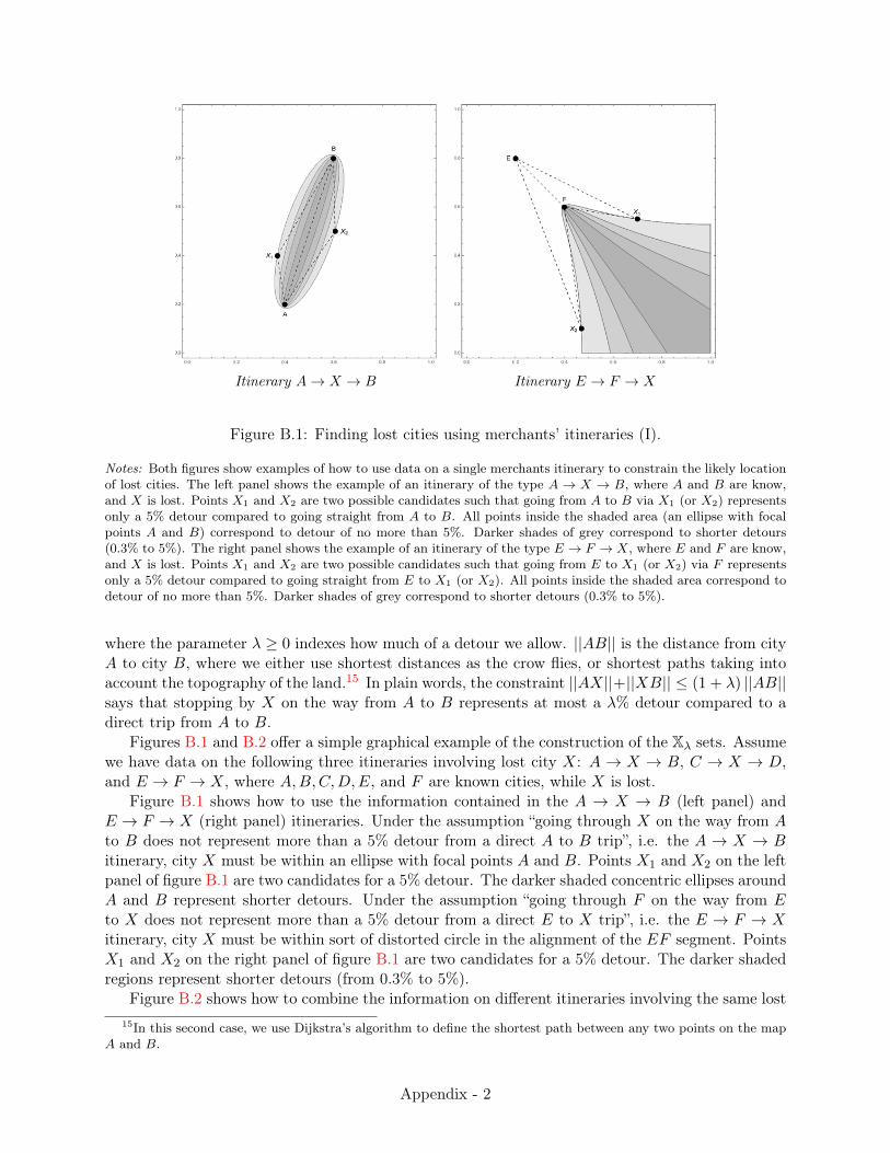
Itinerary A→ X → B Itinerary E → F → X

Figure B.1: Finding lost cities using merchants’ itineraries (I).

Notes: Both figures show examples of how to use data on a single merchants itinerary to constrain the likely locationof lost cities. The left panel shows the example of an itinerary of the type A → X → B, where A and B are know,and X is lost. Points X1 and X2 are two possible candidates such that going from A to B via X1 (or X2) representsonly a 5% detour compared to going straight from A to B. All points inside the shaded area (an ellipse with focalpoints A and B) correspond to detour of no more than 5%. Darker shades of grey correspond to shorter detours(0.3% to 5%). The right panel shows the example of an itinerary of the type E → F → X, where E and F are know,and X is lost. Points X1 and X2 are two possible candidates such that going from E to X1 (or X2) via F representsonly a 5% detour compared to going straight from E to X1 (or X2). All points inside the shaded area correspond todetour of no more than 5%. Darker shades of grey correspond to shorter detours (0.3% to 5%).

where the parameter λ ≥ 0 indexes how much of a detour we allow. ||AB|| is the distance from cityA to city B, where we either use shortest distances as the crow flies, or shortest paths taking intoaccount the topography of the land.15 In plain words, the constraint ||AX||+||XB|| ≤ (1 + λ) ||AB||says that stopping by X on the way from A to B represents at most a λ% detour compared to adirect trip from A to B.

Figures B.1 and B.2 offer a simple graphical example of the construction of the Xλ sets. Assumewe have data on the following three itineraries involving lost city X: A → X → B, C → X → D,and E → F → X, where A,B,C,D,E, and F are known cities, while X is lost.

Figure B.1 shows how to use the information contained in the A → X → B (left panel) andE → F → X (right panel) itineraries. Under the assumption “going through X on the way from Ato B does not represent more than a 5% detour from a direct A to B trip”, i.e. the A → X → Bitinerary, city X must be within an ellipse with focal points A and B. Points X1 and X2 on the leftpanel of figure B.1 are two candidates for a 5% detour. The darker shaded concentric ellipses aroundA and B represent shorter detours. Under the assumption “going through F on the way from Eto X does not represent more than a 5% detour from a direct E to X trip”, i.e. the E → F → Xitinerary, city X must be within sort of distorted circle in the alignment of the EF segment. PointsX1 and X2 on the right panel of figure B.1 are two candidates for a 5% detour. The darker shadedregions represent shorter detours (from 0.3% to 5%).

Figure B.2 shows how to combine the information on different itineraries involving the same lost15In this second case, we use Dijkstra’s algorithm to define the shortest path between any two points on the map

A and B.

Appendix - 2

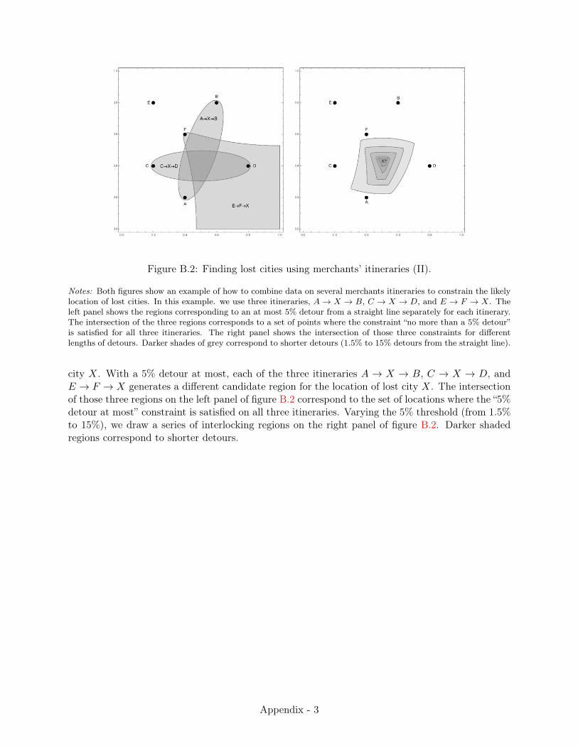
Figure B.2: Finding lost cities using merchants’ itineraries (II).

Notes: Both figures show an example of how to combine data on several merchants itineraries to constrain the likelylocation of lost cities. In this example. we use three itineraries, A→ X → B, C → X → D, and E → F → X. Theleft panel shows the regions corresponding to an at most 5% detour from a straight line separately for each itinerary.The intersection of the three regions corresponds to a set of points where the constraint “no more than a 5% detour”is satisfied for all three itineraries. The right panel shows the intersection of those three constraints for differentlengths of detours. Darker shades of grey correspond to shorter detours (1.5% to 15% detours from the straight line).

city X. With a 5% detour at most, each of the three itineraries A → X → B, C → X → D, andE → F → X generates a different candidate region for the location of lost city X. The intersectionof those three regions on the left panel of figure B.2 correspond to the set of locations where the “5%detour at most” constraint is satisfied on all three itineraries. Varying the 5% threshold (from 1.5%to 15%), we draw a series of interlocking regions on the right panel of figure B.2. Darker shadedregions correspond to shorter detours.

Appendix - 3

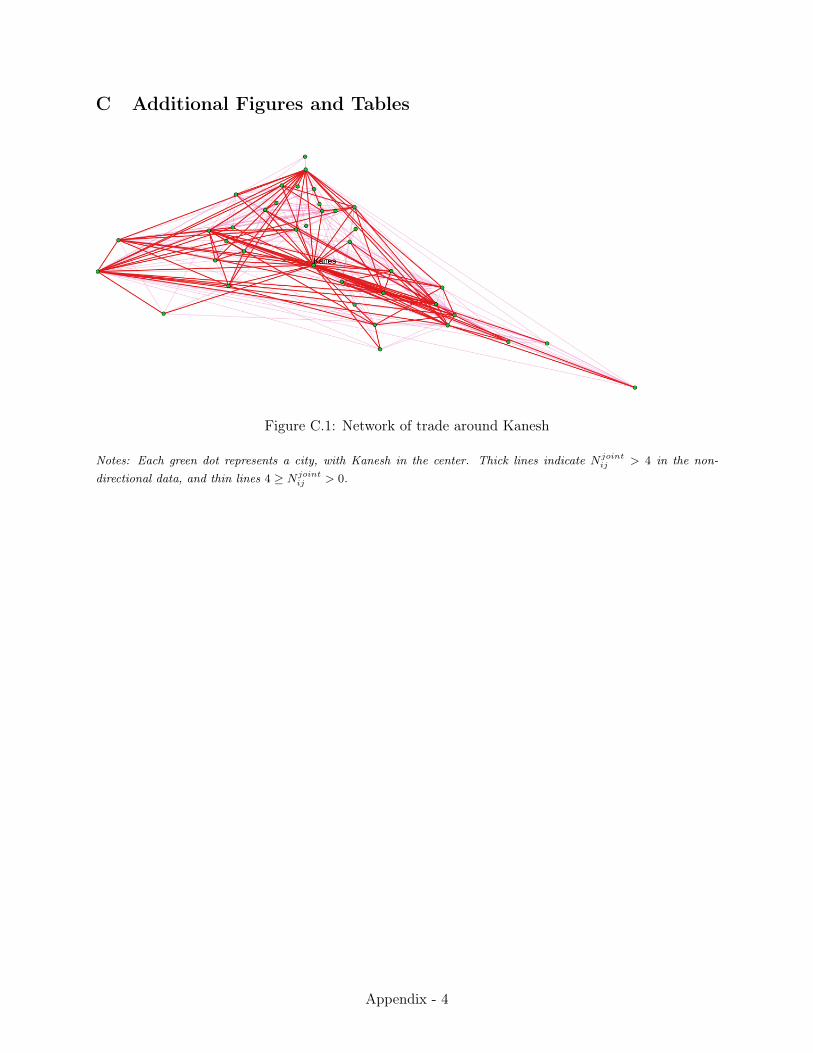
C Additional Figures and Tables

Figure C.1: Network of trade around Kanesh

Notes: Each green dot represents a city, with Kanesh in the center. Thick lines indicate N jointij > 4 in the non-

directional data, and thin lines 4 ≥ N jointij > 0.

Appendix - 4

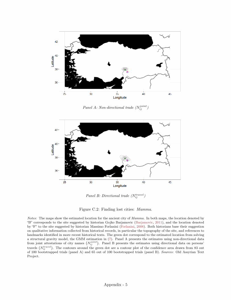
Panel A: Non-directional trade (N jointij )

Panel B: Directional trade (N travelij )

Figure C.2: Finding lost cities: Mamma.

Notes: The maps show the estimated location for the ancient city of Mamma. In both maps, the location denoted by“B” corresponds to the site suggested by historian Gojko Barjamovic (Barjamovic, 2011), and the location denotedby “F” to the site suggested by historian Massimo Forlanini (Forlanini, 2008). Both historians base their suggestionon qualitative information collected from historical records, in particular the topography of the site, and references tolandmarks identified in more recent historical texts. The green dot correspond to the estimated location from solvinga structural gravity model, the GMM estimation in (7). Panel A presents the estimates using non-directional datafrom joint attestations of city names

(N jointij

). Panel B presents the estimates using directional data on persons’

travels(N travelij

). The contours around the green dot are a contour plot of the confidence area drawn from 83 out

of 100 bootstrapped trials (panel A) and 65 out of 100 bootstrapped trials (panel B). Sources: Old Assyrian TextProject.

Appendix - 5

Panel A: Non-directional trade (N jointij )

Panel B: Directional trade (N travelij )

Figure C.3: Finding lost cities: Ninassa.

Notes: The maps show the estimated location for the ancient city of Ninassa. In both maps, the location denoted by“B” corresponds to the site suggested by historian Gojko Barjamovic (Barjamovic, 2011), and the location denotedby “F” to the site suggested by historian Massimo Forlanini (Forlanini, 2008). Both historians base their suggestionon qualitative information collected from historical records, in particular the topography of the site, and references tolandmarks identified in more recent historical texts. The green dot correspond to the estimated location from solvinga structural gravity model, the GMM estimation in (7). Panel A presents the estimates using non-directional datafrom joint attestations of city names

(N jointij

). Panel B presents the estimates using directional data on persons’

travels(N travelij

). The contours around the green dot are a contour plot of the confidence area drawn from 83 out

of 100 bootstrapped trials (panel A) and 65 out of 100 bootstrapped trials (panel B). Sources: Old Assyrian TextProject.

Appendix - 6

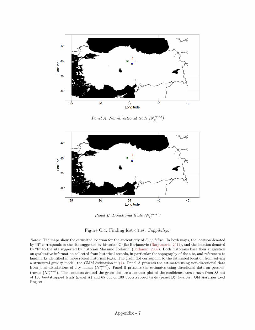
Panel A: Non-directional trade (N jointij )

Panel B: Directional trade (N travelij )

Figure C.4: Finding lost cities: Suppiluliya.

Notes: The maps show the estimated location for the ancient city of Suppiluliya. In both maps, the location denotedby “B” corresponds to the site suggested by historian Gojko Barjamovic (Barjamovic, 2011), and the location denotedby “F” to the site suggested by historian Massimo Forlanini (Forlanini, 2008). Both historians base their suggestionon qualitative information collected from historical records, in particular the topography of the site, and references tolandmarks identified in more recent historical texts. The green dot correspond to the estimated location from solvinga structural gravity model, the GMM estimation in (7). Panel A presents the estimates using non-directional datafrom joint attestations of city names

(N jointij

). Panel B presents the estimates using directional data on persons’

travels(N travelij

). The contours around the green dot are a contour plot of the confidence area drawn from 83 out

of 100 bootstrapped trials (panel A) and 65 out of 100 bootstrapped trials (panel B). Sources: Old Assyrian TextProject.

Appendix - 7

Panel A: Non-directional trade (N jointij )

Panel B: Directional trade (N travelij )

Figure C.5: Finding lost cities: Hahhum.

Notes: The maps show the estimated location for the ancient city of Hahhum. In both maps, the location denoted by“B” corresponds to the site suggested by historian Gojko Barjamovic (Barjamovic, 2011), and the location denotedby “F” to the site suggested by historian Massimo Forlanini (Forlanini, 2008). Both historians base their suggestionon qualitative information collected from historical records, in particular the topography of the site, and references tolandmarks identified in more recent historical texts. The green dot correspond to the estimated location from solvinga structural gravity model, the GMM estimation in (7). Panel A presents the estimates using non-directional datafrom joint attestations of city names

(N jointij

). Panel B presents the estimates using directional data on persons’

travels(N travelij

). The contours around the green dot are a contour plot of the confidence area drawn from 83 out

of 100 bootstrapped trials (panel A) and 65 out of 100 bootstrapped trials (panel B). Sources: Old Assyrian TextProject.

Appendix - 8

Panel A: Non-directional trade (N jointij )

Panel B: Directional trade (N travelij )

Figure C.6: Finding lost cities: Kuburnat.

Notes: The maps show the estimated location for the ancient city of Kuburnat . In both maps, the location denotedby “B” corresponds to the site suggested by historian Gojko Barjamovic (Barjamovic, 2011), and the location denotedby “F” to the site suggested by historian Massimo Forlanini (Forlanini, 2008). Both historians base their suggestionon qualitative information collected from historical records, in particular the topography of the site, and references tolandmarks identified in more recent historical texts. The green dot correspond to the estimated location from solvinga structural gravity model, the GMM estimation in (7). Panel A presents the estimates using non-directional datafrom joint attestations of city names

(N jointij

). Panel B presents the estimates using directional data on persons’

travels(N travelij

). The contours around the green dot are a contour plot of the confidence area drawn from 83 out

of 100 bootstrapped trials (panel A) and 65 out of 100 bootstrapped trials (panel B). Sources: Old Assyrian TextProject.

Appendix - 9

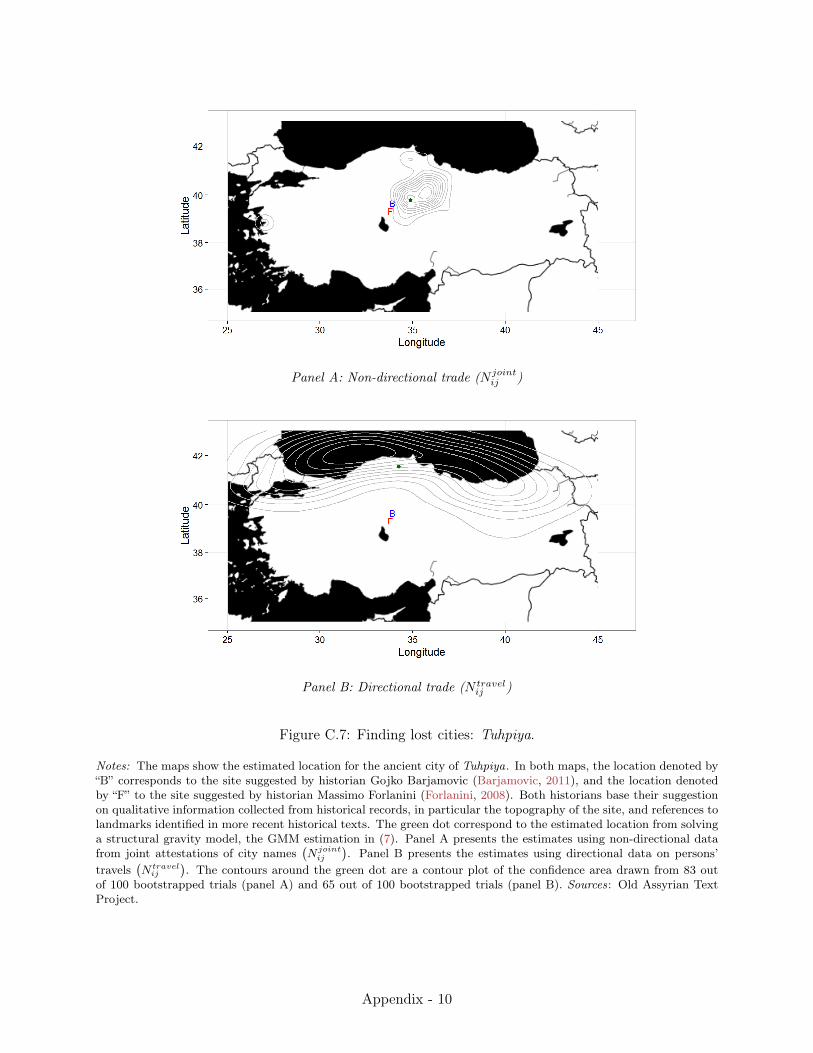
Panel A: Non-directional trade (N jointij )

Panel B: Directional trade (N travelij )

Figure C.7: Finding lost cities: Tuhpiya.

Notes: The maps show the estimated location for the ancient city of Tuhpiya. In both maps, the location denoted by“B” corresponds to the site suggested by historian Gojko Barjamovic (Barjamovic, 2011), and the location denotedby “F” to the site suggested by historian Massimo Forlanini (Forlanini, 2008). Both historians base their suggestionon qualitative information collected from historical records, in particular the topography of the site, and references tolandmarks identified in more recent historical texts. The green dot correspond to the estimated location from solvinga structural gravity model, the GMM estimation in (7). Panel A presents the estimates using non-directional datafrom joint attestations of city names

(N jointij

). Panel B presents the estimates using directional data on persons’

travels(N travelij

). The contours around the green dot are a contour plot of the confidence area drawn from 83 out

of 100 bootstrapped trials (panel A) and 65 out of 100 bootstrapped trials (panel B). Sources: Old Assyrian TextProject.

Appendix - 10

Panel A: Non-directional trade (N jointij )

Panel B: Directional trade (N travelij )

Figure C.8: Finding lost cities: Zalpa.

Notes: The maps show the estimated location for the ancient city of Zalpa. In both maps, the location denoted by“B” corresponds to the site suggested by historian Gojko Barjamovic (Barjamovic, 2011), and the location denotedby “F” to the site suggested by historian Massimo Forlanini (Forlanini, 2008). Both historians base their suggestionon qualitative information collected from historical records, in particular the topography of the site, and references tolandmarks identified in more recent historical texts. The green dot correspond to the estimated location from solvinga structural gravity model, the GMM estimation in (7). Panel A presents the estimates using non-directional datafrom joint attestations of city names

(N jointij

). Panel B presents the estimates using directional data on persons’

travels(N travelij

). The contours around the green dot are a contour plot of the confidence area drawn from 83 out

of 100 bootstrapped trials (panel A) and 65 out of 100 bootstrapped trials (panel B). Sources: Old Assyrian TextProject.

Appendix - 11