Trade, Quality Upgrading and Wage Inequality

in the Mexican Manufacturing Sector: Theory

and Evidence from an Exchange-Rate Shock

Eric VerhoogenColumbia Universityev2124@columbia.edu

Jan. 2004

Abstract

This paper proposes a new model of the link between expanding trade and rising wage inequalityin developing countries, and investigates its causal implications in a newly constructed panel ofMexican manufacturing establishments. In a theoretical setting with heterogeneous firms andquality differentiation, only the most productive firms in a developing country like Mexico enterthe export market, and they produce a better-quality good for export than for the domesticmarket in order to appeal to richer developed-country consumers. Producing high-quality goodsrequires paying high wages both to white-collar and to blue-collar — but especially to white-collar— employees. An increase in the incentive for developing-country producers to export generatesdifferential quality upgrading within industries, as more-productive firms increase exports andproduce a greater share of high-quality goods, while less-productive firms remain focused on thedomestic market. This process raises wage inequality both between firms and within the firmsthat upgrade. The empirical part of the paper uses a major exchange rate shock — the Mexicanpeso crisis of late 1994 — to test this causal mechanism. I find robust evidence that during theyears of the crisis initially more-productive plants increased white-collar wages, blue-collar wages,and the relative wage of white-collar workers as compared to initially less-productive plants inthe same industry. This pattern is absent in the periods before and after the crisis years. Theresults thus support the hypothesis that differential quality upgrading induced by the exchangerate shock contributed to the increase in wage inequality in Mexico in the mid-1990s.

Acknowledgments

Over the course of this project, I have incurred debts that will be a long time in repayment.I would like to thank: Abigail Duran, Adriana Ramirez, Aracely Martinez, Eduardo Sanchez,Ramon Sanchez, Gabriel Romero, Alejandro Cano and Ricardo Magdalena Aguinaga of INEGIfor tireless assistance with the establishment surveys; Gerardo Durand, Oswaldo Lopez, LuisHernandez, Mario Pina, Enrique Dussel Peters, Ernesto Lopez Cordoba, Ricardo Vera, JohnRomalis and Jim Tybout for further generous help with data; Gerardo Esquivel of the Colegio deMexico for facilitating data access and giving me a home base in Mexico City; Alfredo Hualde,Daniel Villavicencio, Martha Diaz, Leonel Gonzalez, Huberto Juarez, Luis Felipe Lopez Calva andAdriana Martinez for helping to arrange plant visits; the many managers who took time to talkto me; Rebeca Wong for crucial support at an early stage, without which the project would nothave been possible; George Akerlof, Andrew Bernard, Clair Brown, Matteo Bugamelli, Ken Chay,Damon Clark, Gabriel Demombynes, Arindrajit Dube, Gordon Hanson, Ann Harrison, PabloIbarraran, Jennifer Kaiser, David Lee, Matt Lewis, Sebastian Martinez, Paco Martorell, JustinMcCrary, Aviv Nevo, Jesse Rothstein, Harley Shaiken, Catha Worthman, seminar participantsat UC Berkeley, and especially the chairs of my dissertation committee, David Card and PranabBardhan, for helpful discussions. I am grateful for funding from the Social Science ResearchCouncil, the UC Institute for Labor and Employment, the UC Berkeley Economics Department,and the UC Institute for Mexico and the United States (UC MEXUS). None of the above hasresponsibility for the shortcomings of the paper.

1 Introduction

Studies have found a coincidence between expanding trade and increasing wage inequality in

many developing countries, including Argentina, Brazil, Chile, Colombia, Costa Rica, Malaysia,

Morocco, Taiwan, and Uruguay.1 Mexico is not an exception to the general pattern. Beginning

with its unilateral trade liberalization in the mid-1980s, Mexico saw rapid increases both in the

volume of trade and in the relative wage of skilled workers (Cragg and Epelbaum, 1996; Han-

son and Harrison, 1999). The rising trend in inequality continued in the mid-1990s, with the

implementation of the North American Free Trade Agreement (NAFTA) and a severe currency

devaluation – the peso crisis – in December 1994. From 1994 to 1995, as the growth of manufac-

turing exports accelerated from 21% to 32% per year, the difference between wages of full-time

male workers at the 90th percentile and 50th percentiles of the wage distribution rose by 6.7%.2

From the perspective of standard trade theory, the coincidence of expanding trade and rising

wage inequality in Mexico is puzzling. The simplest version of the Hecksher-Ohlin model of trade

predicts that wage inequality will fall in a country abundant in unskilled labor, as production

shifts toward unskilled-labor-intensive industries, raising the demand for unskilled workers. More

sophisticated Hecksher-Ohlin-type models can account for a link between trade liberalization and

wage inequality in a developing country like Mexico.3 But because such models focus exclusively

on between-sector shifts as the mechanism through which trade affects labor markets4, they can

only explain a rise in inequality if trade causes a shift toward skilled-labor-intensive sectors. This

condition is violated in the Mexican case. Figures 1a and 1b plot the change in employment

over the period 1988-1998 by 4-digit manufacturing industries against measures of the level of

skill- and capital-intensity. Both figures reveal a clear shift toward industries intensive in the use

of unskilled labor, consistent with the simplest Hecksher-Ohlin story. The apparent inability of

conventional trade theories to explain the rising relative wage of skilled workers in developing

1 See Galiani and Sanguinetti (2003) on Argentina; Blom et al (2001), Green et al (2001), and Pavcnik et al(2002) on Brazil; Robbins (1994), Gindling and Robbins (2001) and Beyer et al (1999) on Chile; Robbins (1996b)and Attanasio et al (2002) on Colombia; Robbins and Gindling (1996) and Gindling and Robbins (2001) on CostaRica. Robbins (1996a), Slaughter (2000), IADB (2002), Harrison and Hanson (1999), and Kremer and Maskin(2003) provide overviews.

2 The calculations are based on the Encuesta Nacional de Empleo Urbano (ENEU), a household survey similarto the U.S. Current Population Survey. The calculation is for full-time male workers, ages 12-64, living in one ofthe 16 cities in the original ENEU sample. In these data, inequality declined slightly in the late 1990s, beginningin 1997. See Esquivel and Rodriguez-Lopez (2003), Hanson (2002) and Robertson (2000) for discussions of recenttrends.

3 We might expect a rise in the relative wage of skilled labor in a country like Mexico, for instance, if thecountry opens trade simultaneously with the U.S. and another country that is even more unskilled-labor-abundant(e.g. China) (Davis, 1996; Wood, 1997); if relatively unskilled-labor-intensive industries are more protected priorto liberalization (Revenga, 1997; Goldberg and Pavcnik, 2001; Feliciano, 2000); or if the production of maize ischaracterized by a factor intensity reversal (Larudee, 1995).

4 An exception is the outsourcing model of Feenstra and Hanson (1996), to which I return below.

1

countries has led many observers to conclude that it must be due to factors unrelated to trade

such as skill-biased technical change (Esquivel and Rodriguez-Lopez, 2003; Meza, 1999) or policy

changes like deregulation and privatization that tend to accompany trade liberalization (Behrman

et al, 2000).5

This paper proposes a new model of the link between trade and wage inequality in developing

countries and tests its causal implications in a newly constructed panel of Mexican manufacturing

plants. In the model, firms are heterogeneous in an underlying productivity parameter (which can

be interpreted as technical know-how or entrepreneurial ability) and goods are differentiated in

quality. Within each industry, only the most productive firms in a developing country like Mexico

enter the export market, and they produce a better-quality good for export than for the domestic

market in order to appeal to richer developed-country consumers. Producing high-quality goods

in turn requires paying high wages to both white-collar and blue-collar employees, but especially

to white-collar employees. An increase in the incentive to export leads to differential quality

upgrading within industries: initially more-productive firms increase exports and shift toward

greater production of higher-quality goods; initially less-productive firms remain solely in the

domestic market and undertake no such upgrading. This process leads initially more-productive

firms to raise wages across occupational categories, to raise the relative wage of white-collar

workers, and to increase capital-intensity relative to initially less-productive firms within the same

industry.

The empirical part of the paper uses the peso devaluation of December 1994 to test the pre-

diction of differential quality upgrading within industries. My econometric strategy issues directly

from the theoretical model. I generate a proxy for the unobserved know-how parameter using

data from before the exchange rate shock, following one of two methods. In the first, I use the log

of domestic sales deviated from industry means, which the model suggests will be proportional to

the know-how parameter. In the second, I take the first principal component of a number of plant

characteristics which the model suggests are correlated with the unobserved parameter. Once the

proxy has been generated, I simply regress changes in plant behavior over the crisis period on the

level of the proxy from before the shock. I find robust evidence that over the 1993-1997 period

initially more productive plants increased the export share of sales, raised wages for both white-

collar and blue-collar workers, raised the relative wage of white-collar workers, and increased the

capital-labor ratio to a greater extent than initially less productive plants. Using an auxiliary

dataset, I also find that over the 1994-1998 period initially more-productive plants were more

5 Several papers have extended the technical-change argument to include the possibility that trade acceleratesthe process of skill-biased technical change, which then generates a rise in the skill premium (Acemoglu 1999;Pissarides 1997, Thoenig and Verdier 2002).

2

likely to acquire ISO 9000 certification, an international production standard commonly associ-

ated with high product quality. As a further test, I re-estimate the same model on periods before

and after the peso crisis during which a currency devaluation did not intervene. I find essentially

no evidence of quality upgrading in the 1989-1993 or the 1997-2001 periods. The only years in

which I find similar (but weaker) results are 1986-1989, a period that itself was characterized by

a significant depreciation of the peso. The results thus provide strong support for the hypothesis

that differential quality upgrading due to the exchange rate shock contributed to the increase in

wage inequality in Mexico in the mid-1990s.

In formalizing the mechanism of differential quality upgrading, the model draws on four el-

ements from the existing theoretical literature.6 The first element is monopolistic competition

with heterogeneous producers, in the spirit of Melitz’s (2003) extension of the seminal papers by

Krugman (1979, 1980).7 The second element is a micro-founded form of differentiation in product

quality, drawn from Anderson et al’s (1992) extension of the discrete-choice theory of McFadden

(1978, 1981). The third element is an asymmetry in consumer demand between two countries,

called North and South. In particular, consumers in North are assumed to be richer and hence

more willing to pay for quality than consumers in South.8 The fourth element is an O-ring pro-

duction function from Kremer (1993) and Kremer and Maskin (1996), in which the production

of high-quality goods requires highly skilled workers across occupational categories and is more

sensitive to the skill of white-collar workers than to that of blue-collar workers.9 The main con-

tribution of the model is to synthesize these previously separate ideas and to elucidate a new

mechanism through which trade-related shocks may affect outcomes at the plant level: shifts in

the within-plant product mix between goods of different qualities destined for different markets.

The empirical part of the paper is related to a growing empirical literature on international

trade and the behavior of individual plants. Studies in this literature have tended to find little

evidence of within-plant changes in behavior in response to exposure to international markets.

6 The idea that trade with developed countries induces quality upgrading in industrial firms in developingcountries is present in, for instance, Morawetz (1981), Gereffi (1999) and Lopez (2003). The contribution of thetheoretical part of this paper is to work out the logic of one rigorous version of the argument.

7 Bernard, Eaton, Jensen and Kortum (2003) present an alternative model that also allows for plant-levelheterogeneity. This paper is also related to a small literature on trade and wages under monopolistic competition,which assume symmetric countries and focus on scale effects as the mechanism through which trade affects relativewages (Dinopoulos and Segerstron, 1999; Dinopoulos et al, 2001; Epifani and Gancia, 2002; Eckholm and MidelfartKnarvik, 2001; Yeaple, 2003).

8 This idea dates back at least to Linder (1961), and has been further elaborated upon by Shaked and Sutton(1982), Flam and Helpman (1987), Stokey (1991), Copeland and Kotwal (1996), Murphy and Shleifer (1997), andBrooks (2003). Hallak (2003), which I became aware of after the first draft of this paper had been circulated, hasrecently incorporated it into a model of trade under imperfect competition.

9 Kremer and Maskin (2003) present a simple O-ring model to explain the coincidence of expanding tradeand rising wage inequality in developing countries, but through matching of Southern and Northern workers inmultinational firms, rather than through the quality-upgrading mechanism emphasized in this paper.

3

An emerging consensus in the literature on trade and productivity is that trade raises aggregate

productivity by shifting production toward more-productive plants, rather than by improving pro-

ductivity within plants (Clerides, Lach, and Tybout, 1998, Bernard and Jensen, 1999).10 Studies

that have examined the effects of industry-level changes in trade policy on plant-level changes in

wage and employment decisions have found what many observers have described as puzzlingly

small effects, in some cases despite large changes in tariffs or other trade policy measures.11 In

contrast, this paper finds strong, robust effects of a shock to the incentive to export on within-

plant behavior. The strength of the results may be due to two advantages of using an exchange

rate shock, rather than changes in trade policy, as the source of exogenous variation.12 First,

unlike most changes in trade policy, the shock was largely unexpected. Second, the shock was big.

The peso lost approximately half of its value in a matter of days at the end of 1994, a change that

dwarfs average tariff changes under NAFTA. This is especially important if we are interested in

shocks to the incentive to export to a rich country. Tariff reductions by developed countries are

typically small, in part because their tariffs tend already to be low. The challenge in making use of

an exchange-rate shock is to identify a source of variation in its impact at the plant level. A main

empirical contribution of this paper is to show how to use the interaction of the exchange-rate

shock and pre-existing heterogeneity within industries to identify the heterogeneous effects of the

shock at the plant level.

The main alternative theory of the link between expanding trade and rising wage inequality in

Mexico is the outsourcing hypothesis of Feenstra and Hanson (1996, 1997). In their model, pro-

duction in each industry is divided into phases of different skill intensities. Capital accumulation

in Mexico leads to the outsourcing of progressively more skill-intensive phases to Mexico within

each industry, raising the overall demand for skill in a way that does not show up in aggregate

between-industry shifts like the ones illustrated by Figure 1. Their model is arguably best applied

to the Mexican maquiladoras, plants legally committed to producing under subcontract for the

export market.13 Both the theory and the empirical work in this paper are primarily concerned

with the non-maquiladora sector, and in this sense the two arguments are complementary. But

10 For a review of the literature on trade and productivity in developing countries, see Tybout (2000).11 Levinsohn sums up his investigations in Chile with the statement: “Try as one might, it is difficult to find any

differential employment response to the trade liberalization.” See also Currie and Harrison (1997) and Harrisonand Hanson (1999).

12 This is not the first paper to use an exchange-rate shock identify an effect of international competition.Previous studies include Revenga (1992), Abowd and Lemieux (1993), and Bertrand (1999). What is new in thispaper is the use of within-industry heterogeneity in the impact of such a shock to estimate its effects.

13 Maquiladoras are plants participating in a government program that until recently required them to exportnearly all of their output in exchange for relief from tariff duties on the value of imported inputs. In Mexico, theparticipants in this program are referred to as maquiladoras de exportacion (exporting maquiladoras). The wordmaquiladora (or maquila for short) is used more generally to apply to any plant producing under sub-contract. Iwill use the term only to refer to the former group.

4

I present two types of evidence that favor the quality-upgrading hypothesis over the outsourc-

ing hypothesis as an explanation for increasing wage inequality in Mexico. First, plants in the

non-maquiladora sector changed wages even in the absence of changes in the proportion of white-

and blue-collar workers used in production, which suggests that the wage changes were not driven

by shifts between activities of different skill-intensities, at least among non-maquiladora plants.

Second, I present evidence (based on micro-data that were unavailable to Feenstra and Hanson)

that maquiladoras are on average markedly less skill-intensive than the rest of the Mexican man-

ufacturing sector. Although there may have been a shift toward more skill-intensive activities

within the maquiladora sector, it appears that the first-order consequence of the expansion of the

sector was an increase in the demand for less-skilled labor.

The next section provides background on the peso crisis and presents a concrete example –

a case study of the Volkswagen plant in Puebla, Mexico – to illustrate the process of quality

upgrading. Section 3 is the theoretical part of the paper. Section 3.1 develops the model for a

closed economy, Section 3.2 sets out the two country version and relates the model to the observable

variables available in the Mexican plant-level data, and Section 3.3 derives the comparative-static

implications of an exchange rate shock for these observables. Section 4 is the empirical part.

Section 4.1 describes the datasets and review broad patterns in the data, Section 4.2 discusses my

econometric strategy, Section 4.3 presents the results, and Section 4.4 presents additional findings

from the auxiliary dataset. Section 5 concludes.

2 Background and Brief Case Study

On Dec. 20, 1994, running short of reserves to defend its exchange-rate target, the new adminis-

tration of Ernesto Zedillo announced that it would raise the ceiling on its exchange-rate band by

15%. This set off a speculative attack and investor flight from the peso, led by domestic Mexi-

can investors. The currency promptly lost approximately 50% of its value, precipitating a major

recession in Mexico. As Figure 2a illustrates, the aggregate price level in Mexico relative to the

price level in U.S. dropped sharply with the devaluation and recovered only slowly thereafter.14

Labor costs in dollar terms followed a similar pattern. Figure 2b plots the average wage level

of full-time male workers with 9 years of education over the period 1993-1999, both in current

U.S. dollars and in current pesos.15 Interestingly, the nominal wages of manufacturing workers

appear to have been almost entirely unaffected. In dollar terms, by contrast, the average wage

14 It is interesting to note that there was a similar real depreciation of the peso in 1986. The 1986-1989 periodwill provide a corroborating test the differential quality upgrading hypothesis in the empirical section below.

15 The data, again, are from the ENEU. See footnote 2.

5

for a male full-time worker with a junior high education fell from approximately $1.50 per hour

to approximately $.90 per hour from 1994 to 1995, rising back only to $1.10 per hour by 1999.

It is worth emphasizing that the peso crisis was a much larger shock than NAFTA, which

had taken effect the previous January. Mexico’s main round of trade liberalization came in the

mid-1980s with its unilateral abandonment of import-substituting industrialization and entrance

into the General Agreement on Tariffs and Trade. By 1993, almost all quotas and other non-tariff

barriers had been removed, and approximately 95% of all imports into Mexico were covered by

tariffs of 20% or less. On the U.S. side, tariffs were initially even lower: approximately 80% of

imports into the U.S. were covered by tariffs of 5% or less. Moreover, the implementation of

NAFTA did not represent a sudden shock. A majority of commodities were assigned phase-out

schedules of five or more years. A common view among observers in Mexico is that NAFTA’s main

role was as a commitment device to the general program of liberalization begun in the 1980s.16

How did the manufacturing sector respond to the crisis? To provide a concrete point of

reference for the theoretical discussion, consider the example of one important plant in Mexico,

the Volkswagen auto plant in Puebla, about two hours south of Mexico City. The Puebla plant

is the sole producer in the world of one of Mexico’s highest-profile exports to the U.S., the New

Beetle. (It is also the sole producer for the U.S. market of another well-known model, the Jetta.)

It comes as something of a surprise, then, that it is relatively rare to see a New Beetle in Mexico.

The streets and highways of Mexico are dominated by the old model, the Original Beetle, known

in Mexico as the Sedan (or, more affectionately, the Vocho), which was produced in the same

plant until July 30, 2003.

The Original Beetle and the newer models, the New Beetle and the Jetta, represent a stark

case of quality differentiation between goods produced primarily for the domestic market and

goods produced primarily for export. The New Beetle and the Jetta have automatic window-

raising mechanisms; the windows of the Original Beetle have to be cranked up by hand. The

seats of the New Beetle and Jetta consist of polyurethane foam; the seats of the Original Beetle

are made partly of foam and partly of coconut fibers, a cheaper substitute. These and other

quality differences are reflected in the prices of the models: the New Beetle and the Jetta sell for

approximately US$17,750 and US$15,000 in Mexico, and roughly comparable prices in the U.S.

The Original Beetle until recently sold for approximately US$7,500 in Mexico.

The example of the Volkswagen plant is especially useful because it is possible to follow changes

16 In unreported results, I find little effect of tariff changes at the industry level on plant level employment, sales,or wages, even when allowing for within-industry heterogeneity in plant-level responses, along the lines of the myempirical approach in this paper. These non-results reinforce the argument that the important shock in this periodwas the peso crisis.

6

in production by product line and see how the shock of the peso crisis affected the product mix

within the plant. At the time of the crisis, the New Beetle had not yet been introduced. (It

was introduced in 1998.) The plant was producing the Original Beetle, destined primarily for

the domestic market, and the Jetta and the Golf (a model from which the New Beetle borrows

the chassis and many underlying components), both destined primarily for export. Figure 3a

plots output for the domestic market, output for the export market and total output over the

period 1988-2002. The effect of the peso crisis is evident: output for the domestic market shrank

precipitously and output for the export market rose in 1995. The net effect on output was

a small decline. This shift was accompanied by a shift in the within-plant product mix away

from the Original Beetle and toward the Jetta and Golf. As Figure 3b illustrates, the Original

Beetle accounted for a significant majority of production for the domestic market, and the drop

in domestic-oriented production primarily reflected a drop in production of the Original Beetle.

Figure 3c illustrates that almost no Original Beetles were exported, either before or after the

crisis. The increase in exports reflected an increase in production for export of Jettas and Golfs

and, later, of New Beetles. Figure 3d capture the key facts: exports as a share of total production

rose from 40% in 1994 to 80% in 1995, and this was accompanied by a shift in product mix from a

cheaper, lower-quality model, the Original Beetle, to more expensive, higher-quality models, the

Jetta and Golf.

What consequences did this shift in product mix have inside the plant? The most striking

characteristic of the Puebla plant, until recently, was the juxtaposition of the production lines for

the New Beetle and Jetta, which rely on state-of-the-art technology, and the production line for

the Original Beetle, which employed essentially the same technology as when the plant opened

in 1964, which had been in use in Germany since the 1950s. The contrast was perhaps most

evident in the welding area (linea de soldadura), which I visited in May 2003. The conveyor belt

on the Original Beetle line had been in continuous operation since 1967. The welding was done by

hand, with sparks flying, and line-workers banged irregularities into shape with hammers. Under

the same roof, perhaps twenty yards away, the welding for the Jetta body was and continues to

be performed entirely by robots; the labor requirements are limited to engineers to program the

robots, and skilled maintenance workers to repair the machines in case of mechanical failure. One

consequence of the shift in product mix, then, was a form of technological upgrading, an increase

in the production-weighted average level of technological sophistication in the plant. This change

occurred not because of an increase in the availability of new technologies, but rather because of

a shift toward greater reliance on technologies that were already in use in the plant.

The employees of the Puebla plant are members of an activist union with a history of mil-

7

itancy,17 and a collective-bargaining agreement has constrained the ability of management to

adjust its labor practices in response to the changing product mix. The shift of production to-

ward the Jetta and Golf/New Beetle lines nevertheless appears to have had consequences for skill

demands and wages. Demand has increased for especialistas (specialists), the skilled production

workers who maintain the automated machines such as the robots in the welding area. A typical

production worker (tecnico) in the plant has a junior high school (secundaria) education. The

especialistas, by contrast, are graduates of a 3-year post-secundaria vocational school that the

company administers on the plant grounds. The starting wage for a tecnico under the 2002-

2004 collective bargaining agreement is 122.87 pesos (US$11.18)18 per day. The starting wage

for an especialista is 195.06 pesos (US$17.74) per day. I was unable to persuade the company to

share detailed data on the number of workers of each type and each salary level working on each

production line, and hence am not able to make definitive statements about the changing skill

composition and earnings of the workforce, but conversations with both the former director of

Human Resources and the president of the Volkswagen union suggest that the relative demand for

especialistas has risen with the share of production making intensive use of automated technology.

At the white-collar level, it appears that the use of software engineers, highly skilled relative to

the supervisors on the Original Beetle line, has increased as well.

Does the example of Volkswagen generalize to the manufacturing sector as a whole? Figures

4a-4c show that, as in the Volkswagen example, the peso crisis induced a significant shift toward

production for export. Figure 4a plots total exports, total domestic sales, and total sales from

the EIA 1993-2001 balanced panel. The increase in exports and the decline in domestic sales are

evident. It is notable that the two effects largely appear to have offset each other, in this sample

of large plants. Figure 4b plots exports as a percentage of total sales; the shift toward exporting

appears in even sharper focus. Figure 4c shows that the increase in the volume of exports was

accompanied by an increase in the fraction of establishments exporting, from 30% in 1993 to

approximately 45% in 1997. The U.S. has long been the overwhelmingly important destination

market for Mexican exports. In 1992, the U.S. was the recipient of 80.6% of Mexican exports;

by 2000, the percentage had risen to 88.7%. Thus the increase in exports largely represents an

increase in sales of Mexican plants on the U.S. market. The Volkswagen example suggests by

extension that the increase in exports to the U.S. was likely to have been accompanied by an

increase in the average quality of goods produced and an upgrading of the industrial workforce in

17 The VW union, the Sindicato Independiente Volkswagen, is independent of the main Mexican labor confed-eration, the Confederacion Mexicana de Trabajadores (CTM), and has a long history of strikes, the most recent in2001. For a concise history, see Hanson and Shapiro (1995).

18 At the Oct. 1, 2003 exchange rate of 10.99 pesos/dollar.

8

exporting plants.

3 Theory

This section develops a model of trade, quality upgrading and wage inequality that formalizes

the salient features of the upgrading process as it has played out at Volkswagen and, anecdotal

evidence suggests, across broad segments of the Mexican manufacturing sector. For expositional

purposes, I begin with the less notation-intensive case of a single, closed economy and then move

on to the more notation-heavy two-country version. I begin by deriving the demand curve facing

each firm and the solution to firms’ optimization problems taking entry decisions as given, and

then solve for entry, given these optimizing decisions.

It is worth emphasizing at the outset that the model has a number of special features. I use

specific functional forms and ignore dynamic issues. Incomes are assumed to be homogeneous

within countries and heterogeneous only across countries. The model is partial-equilibrium, im-

plicitly focused on a single differentiated-goods industry that is small relative to the economy as

a whole in either country. Nonetheless, my hope is that these sacrifices of mathematical elegance

on one hand and realism on the other are justified by the extent to which the model achieves

two goals: to bring the insights of new trade theory – which, in assuming symmetric countries,

has implicitly been focused on integration among developed countries – to bear on the distinctive

experience of developing countries; and to tie the model directly to an empirical approach capable

of estimating its causal implications in real data on Mexican plants.

3.1 One-Country Model

3.1.1 Demand

There are N statistically identical consumers, indexed by i. Each is assumed to buy one unit of

some variety, with varieties indexed by j, for j = 1..J. Each has the indirect utility function:

Vij = θqj − pj + εij (1)

The variables qj and pj are the quality (observable to the consumer) and price of variety

j, respectively. The parameter θ captures consumers’ willingness to pay for quality. It can be

interpreted as a function of income. If richer consumers have identical utility functions as poorer

consumers but the marginal utility of income is declining, they will be willing to pay more for a

9

given level of quality.19 I assume that θ is constant across consumers within a country, and differs

only across countries. I treat it as a fixed parameter, and abstract from changes in consumers’

willingness to pay for quality arising from income changes due to the peso crisis.

The individual-specific random-utility terms, εij, are assumed to have identical double-exponential

distributions and to be independent across goods and consumers. Except for the quality term,

the set-up is a standard multinomial-logit model of consumer demand (McFadden 1978, 1981).

This particular specification appears in Anderson et al (1992).20 Appendix A.1 shows that this

specification yields the following expected demand for each good j:

E (xj) =N exp [(θqj − pj) /µ]∑Jt=1 exp [(θqt − pt) /µ]

(2)

The parameter µ here captures the degree of differentiation between goods. As µ → 0, any

quality or price difference between goods will be magnified, such that the most attractive good

will capture all the demand, and the model approaches perfect competition.21

As Anderson et al (1992) point out, the resulting model of demand combines horizontal dif-

ferentiation, in the sense that if the prices of all goods are equal each will be purchased with

positive probability, with vertical differentiation, in sense that if the prices of all goods are equal

higher-quality goods will be purchased with a higher probability. The advantage of this approach

is that it allows us to consider large numbers of heterogeneous firms in a tractable way. This

feature distinguishes the monopolistic-competition approach from standard models of differenti-

ation along a single, vertical quality dimension (Gabszewicz and Thisse, 1979, 1980, Gabszewicz

et al, 1981; Shaked and Sutton, 1982; Gabszewicz and Turrini, 2000) which quickly become in-

tractable with more than two firms; from patent-race models in which a single firm captures the

market for an entire industry (Grossman and Helpman, 1991a, 1991b); and from Ricardian-type

vertical-differentiation models based on constant returns to scale and perfect competition (Falvey

and Kierzkowski, 1987; Flam and Helpman, 1987; and Stokey, 1991), which do not specify the

boundaries between individual firms and hence do not carry implications for firm- or plant-level

19 Following Tirole (2000, p. 97 fn 1), if consumers have direct utility Uij = u (x0) + qj + εij where x0 isthe consumption of a non-differentiated numeraire good, then optimization yields the indirect utility function

Vij = u (y − pj) + qj + εij . If pj is small relative to the consumer’s income, y, then a first-order expansion of the

sub-utility function u (·) gives: Vij = u (y) − pju′ (y) + qj + εij . Let θ ≡ 1/u′ (y) , Vij ≡ u′ (y) Vij , εij ≡ u′ (y) εij .The u (y) term will drop out of the expression for aggregate demand, and is for that reason immaterial. We thushave (1).

20 Anderson and de Palma (2001) extend the framework to the case of asymmetric firms choosing different qualitylevels, but do not apply it to the analysis of international trade. Hallak (2003) presents a similar specification in atrade context, but assumes goods have the same quality level within industries and uses the model to analyze thepattern of trade at the industry level, rather than within-industry heterogeneity.

21 In this sense, the parameter µ is analogous to the constant elasticity of substitution parameter in the better-known Dixit-Stiglitz (1977) approach.

10

behavior.22

3.1.2 Production

There is a mass M of firms, heterogeneous in a productivity parameter λ distributed continuously

over the interval [0, λmax], with probability distribution g (λ). As mentioned above, we can think of

λ as representing technical know-how or entrepreneurial ability in the firm.23 (I will use the terms

know-how and productivity interchangeably to refer to this parameter.) I assume that know-how

is a fixed characteristic of the firm,24 and is not available (or is prohibitively costly) on the open

market. The parameter λ uniquely identifies firms within the country.

I assume that production is governed by an O-ring production function. In Kremer’s original

O-ring paper (Kremer, 1993), the production process is divided into a fixed number of tasks,

and output is a multiplicative function of the skill-levels of the workers employed in each task.25

Kremer and Maskin (1996) extend this framework to the case where there are two categories of

workers, which I will refer to as white-collar and blue-collar, and output is given by a Cobb-

Douglas function with a larger coefficient on the skill of the white-collar worker. I adopt the

Kremer-Maskin framework, with four modifications.

First, I separate the quality and the quantity of output. I assume that quantity is determined

by a simple fixed-coefficient production function, with one white-collar and one blue-collar worker

producing one unit of output.26 The empirical part of the paper will present evidence that the

assumption of fixed proportions of white-collar and blue-collar workers is not unreasonable. I

assume that quality is given by a Cobb-Douglas function of the skill-levels of the two workers.

Second, I allow for three alternative interpretations of the “skill” of workers that enters the

quality equation: (1) Workers are heterogeneous in skill levels and firms must pay higher wages to

attract high-skill workers to the firm, as in Kremer’s original paper. (2) Workers are homogeneous

22 Manasse and Turrini (2001) also combine quality differentiation with a model of trade under monopolisticcompetition and frame their results in terms of wage inequality. Three issues limit the usefulness of their modelin this context, however. First, it is not clear how to relate the utility function of their representative consumerto the choices of individual consumers, and hence not clear how to derive differences in aggregate quality demandsfrom individual income differences. Second, product quality in their model is a deterministic function of fixedfirm characteristics, rather than a choice variable of the firm. Third, each firm employs only one employee andthe employee receives all the rents from production. It thus seems more natural to think of these individuals asentrepreneurs rather than employees, and of dispersion of their payoffs as dispersion in profits rather than dispersionin wages.

23 Lucas (1978) posits a similar underlying characteristic of firms and describes it as “managerial talent.”24 An interesting direction for future work is to relax this assumption and allow know-how to evolve at different

rates over time depending on the type of goods the firm produces, in the spirit of the learning-by-doing model ofYoung (1991).

25 The idea is that in sophisticated products, mistakes in any aspect of the production process – for instance,the O-rings in the Space Shuttle Challenger – can drastically reduce the value of the product.

26 In this sense, the model is distinct from existing Hecksher-Ohlin and Ricardian trade models, which rely ondifferences in the proportions of different types of workers across industries (or production phases within industriesin the Feenstra-Hanson model).

11

and skills are firm-specific; acquiring skill is costly because firms must pay to train workers. (3)

Workers are homogeneous and “skill” represents the degree of effort or care exercised in production,

rather than a particular capability or body of knowledge, as in the efficiency-wage theories of

Akerlof (1982), Bowles (1985) or Shapiro and Stiglitz (1984).27 A realistic model would probably

combine all three of these interpretations. For present purposes, the important point is simply

that “skill” improves quality and is costly to the firm to acquire.

Third, I include an additional input, machines. Because we typically only know the total value

of machinery, rather than the number of machines and their level of sophistication separately, it is

not obvious how machines should enter the quantity and quality equations. Here I assume that one

white-collar and one blue-collar worker always combine with one machine, and that the capital-

labor ratio, given by k, enters the quality equation as a proxy for the technical sophistication of

the machine.28

Fourth, I assume that the know-how parameter λ enters as a multiplicative coefficient in the

production function for quality. For the sake of simplicity, I exclude it from the function for

quantity, although this is not crucial.29

Let h and l index white-collar and blue-collar workers. Let eh and el represent the skill or

effort of white-collar workers and blue-collar worker, respectively. Let wh and wl represent the

wages paid by the firm, and wh and wl the outside market wages for each type of worker, which

are taken to be exogenous to the industry being modeled.30 In the interests of simplicity, I assume

that skill/effort level is a linear function of the difference between the wage in the firm and the

outside wage:

eh (λ) = zh[wh (λ)− wh

](3)

el (λ) = zl[wl (λ) −wl

]where zh and zl are positive constants. The production function for quality is given by:

q (λ) = λ [k (λ)]αk [

eh (λ)]αh [

el (λ)]αl

(4)

27 See also Dalmazzo (2002), who integrates this efficiency-wage idea explicitly into the model of Kremer (1993).28 None of the qualitative results in the paper depend on this assumption. Capital is included in the model

mainly to generate implications for a variable on which we will have data, and could easily be dropped.29 A model in which know-how does not affect quality directly but instead reduces input requirements in the

quantity equation for the two types of labor (which affect quality) but not for other costs such as transport or rawmaterials that do not affect quality would generate similar results, at the cost of messier algebra.

30 In interpretations (2) and (3) above, this market wage is the wage that a worker in the firm would actuallyreceive in the outside market. In (1), we can think of it as an average wage among the heterogeneous workers inthe outside market, rather than the wage that a worker in the firm would actually receive if she left the firm.

12

Let α ≡ αk + αh + αl. Assume that improvements to quality from a given increase in the skill

and sophistication of inputs are diminishing: α < 1. This ensures an interior solution in the choice

of quality. Let r be the rental cost of capital. The marginal cost of producing one unit of output,

which by assumption is independent of the quantity produced, is mc (λ) = wh (λ)+wl (λ)+rk (λ).

There is a fixed cost of entry, f .

The combination of constant marginal cost (conditional on quality) and the fixed cost of entry

generates increasing returns to scale. There is no cost to differentiation and firms are constrained

to offer just one variety. As a consequence, all firms differentiate and have a monopoly in the

market for their particular variety. The fixed parameter λ thus indexes goods as well as firms.

Since λ is distributed continuously, we can think of the number of goods J in equation (2) as

going to infinity. Then assuming firms are risk-neutral and dropping the expectation, the demand

function for each good (2) can be rewritten:

x (λ) =N

Dexp

[θq (λ)− p (λ)

µ

](5)

with

D ≡∫

λ∈Λ

exp[θq (λ) − p (λ)

µ

]Mg (λ) dλ (6)

where Λ is the set of firms that enter the market.

3.1.3 Firms’ Optimization

Each firm seeks to maximize its profit: π (λ) = [p (λ)−mc (λ)] x (λ) − f . The firm’s choice

variables are wh, wl, k (which together determine quality, q) and p. As is standard in monopolistic

competition models, I assume that each firm thinks of itself as small relative to the market as a

whole, and treats the aggregate quantity in the denominator of the expression for output, D, as

unaffected by its own choices. Given this assumption, optimization yields:

wh∗ (λ)− wh = αh [ηλθ]1

1−α

wl∗ (λ)−wl = αl [ηλθ]1

1−α (7)

k∗ (λ) =αk

r[ηλθ]

11−α

where η ≡(

αk

r

)αk (zhαh

)αh (zlαl

)αl

. These choices for wages and the capital-labor ratio

determine the quality level:

q∗ (λ) = [ηλθα]1

1−α (8)

13

It is convenient to write the firm’s choice variables in terms of the resulting value of quality:

wh∗ (λ) = wh + αhθq∗ (λ)

wl∗ (λ) = wl + αlθq∗ (λ) (9)

k∗ (λ) =αk

rθq∗ (λ)

The quality of goods produced by the firm is a summary indicator that captures the dependence

of wages and the capital-labor ratio on the firm’s underlying know-how. Equations (8) and (9)

give us our first key implications of the model: in cross-section, higher-λ firms produce higher-

quality goods, pay higher wages to both white-collar and blue-collar workers, and are more capital-

intensive than lower-λ firms. Note also that quality, wages and capital intensity are greater, the

greater the willingness of consumers to pay for quality, θ.

Appendix A.2 shows that the wage ratio: ω∗ (λ) ≡ wh∗(λ)wl∗(λ) is increasing in λ and θ if (and only

if) αh/αl > wh/wl, that is, if the production of quality is sufficiently more sensitive to the skill of

white-collar workers than to that of blue-collar workers.

Marginal cost and price at the optimum are given by mc∗ (λ) = wh + wl + αθq∗ (λ) and

p∗ (λ) = µ + wh +wl +αθq∗ (λ). Note that both are increasing in λ and θ. As is standard in logit

demand models, the mark-up is constant: p∗ (λ)−mc∗ (λ) = µ.

Define I∗ (λ) ≡ [θq∗ (λ)− p∗ (λ)] /µ =[(1− α) (ηθλ)

11−α − µ −wh −wl

]/µ and note that I (·)

is increasing in λ and θ as well. Output and profit can be written:

x∗ =N

D∗ exp I∗ (λ) (10)

π∗ (λ) =µN

D∗ exp I∗ (λ) − f (11)

where

D∗ =∫

λ∈Λ

exp I∗ (λ)Mg (λ) dλ (12)

Equations (10) and (11) complete the set of cross-sectional implications in the one-country

version of the model: taking as given the set Λ of firms that enter, output and profit are greater

for firms with higher λ.

A corollary of equations (7) and (10) is that the size of a firm will be correlated with the wages

it pays to both types of workers, since both are increasing in λ. The model thus provides a natural

14

explanation for the employer size-wage effect, documented by Brown and Medoff (1989) for the

U.S. and by Velenchik (1997) and Schaffner (1998), among others, for developing countries.

3.1.4 Entry

The fact that profitability is increasing in λ implies that in equilibrium there will be a single

cut-off value of productivity, call it λmin, above which all firms will enter and earn positive profits,

and below which no firms will enter. The cut-off is defined implicitly by the requirement that the

marginal firm have zero profits:

π∗(λmin

)=

µN

D∗(λmin

) exp

I∗(λmin

)− f = 0 (13)

where now we can specify the limits of integration for D∗ and write it as a function of the

variable lower cut-off, λmin:

D∗(λmin

)=

∫ λmax

λminexp I∗ (λ)Mg (λ) dλ (14)

Note that D∗ (·) is a decreasing function of λmin: the higher is the cut-off, the smaller the mass

of firms over which we integrate.

3.2 Two-Country Model

3.2.1 Modifications to Basic Set-up

Now suppose that there are two countries in the model, North and South, indexed by n and s.

I assume that the two markets are segmented, in the sense that firms can sell a different quality

product and charge a different price in each market.31 The key difference between countries, as

mentioned above, is that Northern consumers are more willing to pay for quality than Southern

consumers: θn > θs.

I also assume production is segmented, in the sense that firms can make different optimization

decisions for production for the Northern market than for production for the Southern market.

It is convenient to think of each firm as producing (or potentially producing) on two different

production lines, one for the domestic market and one for export.32 We thus potentially have two

31 Firms are still constrained to sell one variety in each market.32 A firm is allowed pay different wages to workers of the same type producing on the different lines. There is thus

no internal equity constraint in this model, although it is likely that in real firms fairness considerations betweenworkers producing on the different lines would constrain firms’ ability to make completely separable decisions onthe two lines.

15

sets of optimization equations for each firm in each country, one for each production line. To keep

track of decisions on each line, I introduce two indices: c = s, n indicates the country in which the

plant is located; and d = s, n indicates the destination market. For variables that pertain either

only to the production location or only to the destination market, I use just one subscript.

The equations governing each firm’s decisions in the one-country model map almost directly

into the equations governing each firm’s decisions on a particular production line, with one main

difference. The ratio of the price levels between the two countries – the real exchange rate – is

allowed to vary. To keep track of these movements, it is convenient to define δcd to be the ratio

of the price level in country d to the price level in country c. Given this definition, we have that

δss = δnn = 1 and δns = 1/δsn. Assume that purchasing power parity holds initially, so that

δsn = δns = 1; below I will assume that a currency shock in South lowers the price level in South

and raises δsn. Consider the price charged by the firm with know-how λ in South for goods sold

on the Northern market. Let psn (λ) be the price charged by the firm in terms of Southern goods.

For Northern consumers the relevant price is the price in terms of Northern goods, which is to

say psn(λ)δsn

. In general, the consumer demand function (equation (5) in the one-country version)

should be rewritten as:

xcd (λ) =Nd

Ddexp

[θdqcd (λ)− pcd(λ)

δcd

µ

](15)

In the two country case, the term in the denominator, Dd, now involves an aggregation in each

consumer market over two sets of firms, domestic firms selling in their home market and foreign

firms exporting to it. Let λmincd represent the cut-off for a firm located in country c to enter

destination market d. Then we can write:

Dd

(λmin

sd , λminnd

)= Dsd

(λmin

sd

)+ Dnd

(λmin

nd

)(16)

where, as in (6),

Dcd

(λmin

cd

)=

∫ λmaxc

λmincd

exp

θdqcd (λ)− pcd(λ)

δcd

µ

Mcgc (λ) dλ (17)

Finally, I assume that firms must pay a fixed cost to export, fe, in addition to the fixed cost

to enter the domestic market. It will be convenient to indicate fixed costs using the subscript

notation: fsn = fss + fe and fns = fnn + fe. The fact that exporters must pay to enter the

domestic market before paying to enter the export market means that there will be no firms that

only enter the export market. The number of consumers in each market, Nn and Ns, the total

masses of firms, Mn and Ms, the distributions of firms, gn (λ) and gs (λ), and the maximum

16

values of entrepreneurial ability, λmaxn and λmax

s , are allowed to differ across countries, although

these differences are of little consequence. The extent-of-differentiation parameter, µ, the cost of

capital, r, the slopes of the skill-wage schedules, zh and zl, and the exponents of the Cobb-Douglas

production function for quality, αh, αl and αk and hence the term η in (7) are assumed not to

differ across countries.

3.2.2 Firms’ Optimization for Each Production Line

Given the two-country set-up, firms’ optimization yields the following (refer to equation (7)):

q∗cd (λ) = [ηλδαcdθα

d ]1

1−α

wh∗cd (λ)− wh

c = αhδcdθdq∗cd (λ)

wl∗cd (λ)−wl

c = αlδcdθdq∗cd (λ)

k∗cd (λ) =αk

rδcdθdq∗cd (λ) (18)

ω∗cd (λ) =wh

c + αhδcdθdq∗cd (λ)

wlc + αlδcdθdq∗cd (λ)

mc∗cd (λ) = whc + wl

c + αδcdθdq∗cd (λ)

p∗cd (λ) = µ + whc + wl

c + αδcdθdq∗cd (λ)

x∗cd (λ) =Nd

D∗d

exp I∗cd (λ)

π∗cd (λ) =µNd

D∗d

exp I∗cd (λ) − fcd

where

I∗cd (λ) ≡[θdq

∗cd −

p∗cd

δcd

]/µ (19)

=[(1− α) (ηλδα

cdθd)1

1−α − µ + whc + wl

c

δcd

]/µ

and D∗d is given by (16) and (17) above.

For each location-destination pair, we have the same set of cross-sectional relationships as in

the one-country case. Among firms in a given country producing for a given market, firms with

greater know-how λ will produce a higher-quality good; pay higher wages to both white-collar

and blue-collar workers; pay a higher relative wage to white-collar workers (conditional on the

assumption that αh/αl > wh/wl); use more capital per worker; charge a higher price; produce

more output and earn more profits.

17

From the expression for quality in (18), we see that if a given firm enters both markets, then

(assuming δss = δsn = 1 initially) it will produce a higher-quality good for the Northern market

than for the Southern one.33 Within each firm, the production of higher-quality goods on the

export line is accompanied by higher wages, higher relative wages of white-collar workers, higher

capital intensity, higher costs, and higher prices than on the production line for the domestic

market.

3.2.3 Entry

In the two-country model, there will be four entry cut-offs, λmincd , one for each location-destination

pair (c = n, s, d = n, s). The cut-offs are determined by four zero-profit conditions:

π∗cd

(λmin

cd

)=

µNd

D∗d

expI∗cd

(λmin

cd

)− fcd = 0 (20)

The fact that firms must first pay the fixed cost to enter the domestic market before paying

the additional fixed cost to export means that λminsn > λmin

ss and λminns > λmin

nn . Within the cross-

section of firms in each country at a given time, we have three distinct groups of firms: firms

that do not enter (call them non-entrants), firms that enter only the domestic market (call them

non-exporters), and firms that enter both markets (call them exporters). In South, non-entrants

correspond to the interval λ ∈ [0, λminss ), non-exporters to the interval λ ∈ [λmin

ss , λminsn ), and

exporters to the interval λ ∈ [λminsn , λmax

s ).

3.2.4 Observables at the Firm Level

The notion of two production lines per firm is conceptually straightforward, but in practical

terms it is rare to have production data on firms or plants by production line, except in particular

industries such as automobiles. This section relates the variables defined above to the variables that

are observable in the Mexican establishment panels and similar datasets. For ease of exposition, I

focus on Southern firms, but the analysis for Northern firms would be analogous. Before deriving

the implications for the observables, it is convenient first to define two variables which are not

directly observable but which will be useful in what follows: the export share of output34 and the

33 A single firm will produce different qualities for different markets even in the absence of the quality bias due toper-unit trade costs first hypothesized by Alchian and Allen (1964). The effect is due solely to differences in qualitydemands by consumers arising from income differences between countries. This phenomenon cannot be capturedin models based on perfect competition in the product market, such as the Ricardian-type quality upgrading modelof Stokey (1991). Under perfect competition, firms face identical product market conditions across countries, andhave no incentive to produce different goods for different markets.

34 The export share of output is not observable because although we observe sales in each market we do notobserve the prices of goods sold on each market, and hence cannot make inferences about the quantities of goodssold.

18

average quality of goods produced.35

Define the export share of output for Southern firms as: χ∗s (λ) ≡ x∗sn(λ)x∗sn(λ)+x∗ss(λ) . Suppose that

all firms enter both markets. Appendix A.3 shows that under this counterfactual assumption

output on each production line is increasing in λ and output on the export line increases more

steeply in λ. Consequently, the export share of output is also increasing in λ. But in general not

all firms enter both markets. For non-exporters, χ∗s (λ) = 0. (For non-entrants, the export share

of output is obviously undefined.) The result that the export share of output is an increasing

function of λ holds only for exporters. Note that there will be a discontinuity in χ∗s (λ) at the cut-

off for entry into the export market. Firms just to the left of the cut-off have zero exports. Firms

just to the right of the cut-off must sell enough on the export market to recoup the indivisible

fixed cost, and have an export share strictly greater than zero.

The average quality of goods produced by a given firm can be expressed as a weighted average

of the quality levels produced on the firm’s two production lines, where the weights are given by

the export share of output: q∗s (λ) = χ∗s (λ) q∗sn (λ)+(1− χ∗s (λ)) q∗ss (λ). Figure 5a summarizes the

relationship between q∗s (λ) and λ in the cross-section of Southern firms. The dashed (as opposed to

dotted) curves represent q∗ss (λ) and q∗sn (λ), the quality levels on each production line. From (18),

we know that q∗ss (λ) and q∗sn (λ) are increasing in λ. Since θn > θs, we also know that the q∗sn (λ)

curve will lie above and have a greater slope than the q∗ss (λ) curve. The dotted curve represents

the counterfactual average quality that would obtain if all firms entered both markets. The solid

curve represents actual average quality as a function of λ. For non-exporters, average quality is

equal to the quality level on the domestic production line, q∗s (λ) = q∗ss (λ). For exporters, the

average quality is given by the dotted curve. Note that the average product quality is increasing

in λ for two reasons: first because product quality is increasing in λ on each production line;

and second because, for the exporters, the export share of output χ∗s (λ) is increasing in λ as

well. There is a discontinuity in average quality at the cut-off for entry into the export market, a

consequence of the discontinuity in the export share of output discussed above.

Wages for each type of worker and capital intensity follow a pattern qualitatively similar to

average quality. The firm-level averages for these variables are given by:

wh∗s (λ) = χ∗s (λ) wh∗

sn (λ) + (1− χ∗s (λ))wh∗ss (λ)

wl∗s (λ) = χ∗swl∗

sn (λ) + (1− χ∗s (λ))wl∗ss (λ)

k∗s (λ) = χ∗s (λ) k∗sn (λ) + (1− χ∗s (λ)) k∗ss (λ)

(21)

35 The data on ISO 9000 certification discussed in section 4.4 provide a partial but clearly incomplete measureof product quality.

19

Like average quality, these variables will be increasing in λ in cross-section, both because wages

and the capital-labor ratio on each production line are increasing in λ and also because the export

share of output is increasing. They will also have a discontinuity at the cut-off for entry into the

export market.

Define the average wage ratio at the firm level as the ratio of the average white-collar wage to

the average blue-collar wage: ω∗s (λ) ≡ wh∗s (λ) /wl∗

s (λ). It can then be rewritten as a weighted

average of the wage ratios on each production line: ω∗s (λ) = χ∗s (λ)ω∗sn (λ) + (1− χ∗s (λ))ω∗ss (λ)

where χ∗s (λ) ≡ χ∗s(λ)wl∗sn(λ)

χ∗s (λ)wl∗sn(λ)+(1−χ∗s(λ))wl∗

ss(λ). Like χ∗s (λ), χ∗s (λ) will be zero for non-exporters and

increasing in λ for exporters. Conditional on the assumption that αh/αl > wh/wl, the wage ratio

will follow the same qualitative pattern as wage levels.

Under the assumption that one white-collar worker and one blue-collar worker are required to

produce one unit of output, employment of each type of worker is simply equal to total output.

Let E represent total employment. For non-exporters, E∗s (λ) = 2x∗ss (λ) and is increasing in λ.

For exporters, E∗s (λ) = 2 (x∗ss (λ) + x∗sn (λ)) and is increasing more steeply in λ. There will also

be a discontinuity in employment at the cut-off for the export market.

The observable variables domestic sales and export sales are distinguished from the other ob-

servables by the fact that they correspond to a single production line. Let S∗ss (λ) = p∗ss (λ)x∗ss (λ)

and S∗sn (λ) = p∗sn (λ) x∗sn (λ) represent domestic sales and exports, respectively. For all firms

that enter the domestic market, non-exporters and exporters, the underlying variables p∗ss (λ) and

x∗ss (λ) – and hence domestic sales, S∗sn (λ) – are continuous, monotonically increasing functions

of λ. I will rely on this fact below, when using domestic sales as a proxy for the underlying pro-

ductivity parameter. Export sales, S∗sn (λ) , are smooth and increasing within the set of exporters,

but are zero for non-exporters, which will make up the majority of plants in our data. Finally, the

export share of sales is given by σ∗s (λ) = S∗sn(λ)S∗ss(λ)+S∗sn(λ) . Appendix A.4 shows that, conditional on

firms entering both markets, the export share of sales is increasing in λ.

3.3 Comparative-Static Effects of an Exchange-Rate Shock

I model the shock as having two (exogenous) effects. First, the real exchange rate, δsn, defined as

the Northern price level over the Southern price level, rises (δns falls). Second, the shock reduces

total consumer demand in South, manifested in our single differentiated goods industry as a decline

in the number of Southern consumers, Ns. In addition, to restrain the proliferation of algebra, I

assume that North is large relative to South, such that the increased entry of Southern firms into

the Northern market in response to the peso crisis does not appreciably affect the profitability of

other firms selling in the Northern market. I focus on the comparative-static effects for Southern

20

firms, since they will be the focus of the empirical work.

3.3.1 Effects on Entry of Southern Firms

The effect of the devaluation of the peso is to make Southern goods more competitive relative to

Northern goods in both markets. Appendix A.5 shows that ∂λminsn /∂δsn < 0 and ∂λmin

ss /∂δsn < 0.

That is, as the real exchange rate rises, more Southern firms will enter both markets. The effect

of the decline in consumer demand in South is to reduce the profitability of all firms selling in

South. Given the segmentation of the consumer markets, it has no effect on the profitability of

selling in North. Formally, Appendix A.5 shows that ∂λminss /∂Ns < 0 and ∂λmin

sn /∂Ns = 0.

The net effect on Southern firms’ entry into the export market is clear: more Southern firms

enter the export market (λminsn falls). The net effect on entry of Southern firms into the South-

ern market is ambiguous: the increased competitiveness of Southern firms and the reduction in

Southern consumer demand work in opposite directions. In fact, the peso crisis led to an increase

in the number of bankruptcies of manufacturing firms in Mexico. It appears that the empirically

relevant case is the one in which λminss rises. The remainder of the paper will focus on this case.

Appendix A.5 gives a precise statement of the condition required to obtain it.

Given our assumptions, the entire continuum of potential firms in South can be classified into

five categories (let pre indicate the pre-crisis period and post the post-crisis period.): (1) Never

entrants (λ < λminss,pre) do not enter either market in either period. (2) Exiters from the domestic

market (λminss,pre ≤ λ < λmin

ss,post) enter only the domestic market in the first period and go out of

business in the second period. (3) Always non-exporters (λminss,post ≤ λ < λmin

sn,post) enter only the

domestic market, in both periods. (4) Switchers into exporting (λminsn,post ≤ λ < λmin

sn,pre) enter only

the domestic market in the first period, but enter both markets in the second period. (5) Always

exporters (λminsn,pre ≤ λ) enter both markets in both periods.

3.3.2 Effects on Production Decisions of Southern Firms

Now consider firm-level production decisions conditional on λ and a given set of entry cut-offs.

Consider first the effect of the crisis on the change in the export share of output. Following the

same approach as in Section 3.3 above, we first calculate the counterfactual export shares of output

assuming that all firms enter both market, both before and after the crisis. Let the change in the

export share be given by dχs (λ) ≡ χs,post (λ) − χs,pre (λ). Appendix A.6 shows that under the

counterfactual that all firms enter both markets, the change in export share of output is given by:

dχs (λ) = Σsχs,pre (λ)[1− χs,pre (λ)

](22)

21

where Σs > 0 and is increasing in λ. Thus dχs (λ) > 0; the export share of output increases

as a result of the shock. In addition, the facts that χs (λ) and Σs are increasing in λ imply that

a sufficient condition for dχs (λ) to be increasing in λ is that χs (λ) < 1/2.36 We will see in the

empirical section that among the minority of Mexican plants that export, the average fraction of

output exported is 20-25%.37 Exports made up more than half of total sales in only 3-7% of plants

over the 1993-2001 period. It thus appears reasonable to focus on the case where χs (λ) < 1/2,

and I do so hereafter. Consider the five cases from above. The never entrants and exiters (Cases

(1) and (2)) are not observed after the crisis. For the always non-exporters (case (3)): dχs (λ) = 0.

For the switchers into exporting (case (4)), the export share is zero before the crisis and positive

after the crisis; the change is dχs (λ) = χs,post (λ). For the always exporters, the change in the

export share is given by (22). Note that dχs (λ) is increasing in λ both within the category of

switchers into exporting and within the category of always exporters, and that there are two

discontinuities in the relationship between dχs (λ) and λ, a jump up at λminsn,pre and a jump down

at λminsn,post.

Now consider the effect on the average quality of goods produced. Suppose again that all firms

enter both markets. Quality on the domestic production line, qss (λ) does not depend on either

δsn or Ns and hence is unaffected by the exchange-rate shock. Quality on the export line, qsn (λ)

increases with the increase in the real exchange rate δsn. Intuitively, the peso devaluation reduces

Southern firms’ cost of producing quality relative to what Northern consumers are willing to pay

for it, and this induces them to supply more of it. Algebraically, we have:

dq∗sn (λ) =(

α

1− α

)[ηλ (θn)α]

11−α (δsn)

2α−11−α dδsn

which is positive and increasing in λ. The increase in the average level of quality in the firm is

then a combination of the increase in the quality on the export line and the increase in the export

share of output:

dqs (λ) = χs (λ) dqsn (λ) + (q∗sn (λ)− q∗ss (λ)) dχs (λ) (23)

Under the counterfactual that firms enter both markets, χs (λ) , dχs (λ) , dqsn (λ) , and q∗sn (λ)−q∗ss (λ) are all positive and increasing in λ; hence dqs (λ) is positive and increasing in λ as well.

Figures 5b depicts the effect of the exchange rate shock on the level average quality. The q∗sn (λ)

36 Intuitively, if a firm is already exporting a large share of output before the shock, then there is little room toincrease the export share further.

37 Moreover, the model suggests that the export share of sales is an upper bound on the export share of output,since the price of output sold in the Northern market is higher than the price of goods sold in South.

22

curve shifts up in response to the shock, and the dotted counterfactual qs (λ) curve also shifts up,

reflecting both the increase in quality on the export line and the increase in the export share of

output. The thinner, dark solid line represents the actual average quality curve pre-crisis. The

thicker, gray solid line represents the actual average quality curve post-crisis. The always non-

exporters continue to produce exclusively for the domestic market and their average quality level

does not change. The switchers into exporting see an especially large increase in average quality.

The always exporters see the change in quality given by equation (23). Figure 5c depicts the change

in average quality as a function of λ. Average quality is increasing in λ within the category of

switchers and within the category of always exporters. There is a positive discontinuity at the

post-crisis cut-off for entry into the export market, λminsn,post, and a negative discontinuity at the

pre-crisis cut-off for entry into the export market, λminsn,pre, both consequences of the discontinuities

in the export share of output.

Recalling (21), the changes in wages for each type of worker and the capital-labor ratio are:

dwh∗s (λ) = χs (λ)αhθnδsndq∗sn (λ) + αh (θnδsnq∗sn (λ)− θsq

∗ss (λ)) dχs (λ)

dwl∗s (λ) = χs (λ)αlθnδsndq∗sn (λ) + αl (θnδsnq∗sn (λ) − θsq

∗ss (λ)) dχs (λ)

dks = χs (λ)(

αk

r

)θnδsndq∗sn (λ) + αk

r(θnδsnq∗sn (λ)− θsq

∗ss (λ)) dχs (λ)

(24)

The pattern of changes in these variables are qualitatively similar to the pattern for average

quality. Note that although I have assumed that outside market wages for each type of worker

are exogenously fixed, it would be straightforward to allow them to vary with the shock. The

important point is that the change in the outside market wage would affect wages in all firms

equally; we would still observe a larger differential increase in higher-λ firms. Appendix A.7

shows that the change in the average wage ratio ωs in response to the shock also follows the same

qualitative pattern as average quality depicted in Figure 5c. Appendix A.8 shows that, for the

case where the export share of sales is less than 1/2, the model carries similar implications for

changes in the export share of sales, σs (λ). Finally, Appendix A.9 shows why the model does not

carry a strong prediction for the effect of the exchange-rate shock on total employment and total

sales. The intuition is that although higher-λ firms see a larger increase in exports, they also have

higher levels of domestic sales prior to the shock and hence a greater drop in domestic sales in

response to the shock.

To sum up, the testable implication I will take to the data is that the pattern illustrated by

Figure 5c will hold for a number of observable variables: wages of each type of worker, the wage

ratio, the capital-labor ratio, the export share of sales, and, to the extent that it is observable,

product quality. Unfortunately, our estimates of λ will be sufficiently imprecise and our data

23

on the these outcome variables will be sufficiently noisy that it will not be possible to estimate

the specific predictions of discontinuities at the post-crisis and pre-crisis cut-offs for entry into

exporting. We will have to content ourselves with estimating roughly linear relationships between

these changes in these observables and estimates of the underlying know-how parameter λ. In this

sense, the empirical work should be seen as testing the first-order qualitative implications of the

model, rather than its specific functional form.

4 Empirics

4.1 Data

The analysis in this paper is based primarily on the Encuesta Industrial Anual (EIA) [Annual

Industrial Survey], a yearly panel survey conducted by the Instituto Nacional de Estadisticas,

Geografia, e Informacion (INEGI), the Mexican government statistical agency. The EIA is a

panel of the largest establishments in Mexico in 205 6-digit manufacturing industries, excluding

maquiladoras. The panel on which the estimates in this paper are primarily based covers the

year 1993-2001. The sample is non-random: In 1993, plants with 100 or more employees were

included with certainty, and smaller plants were included in descending order of size until 85% of

the production of the industry was covered. These plants were then followed over time. Because

of this design, the survey is not appropriate for analyzing shifts in production across industries or

turnover of plants, but it is well-suited to a study of the evolution of the behavior of individual

establishments over time. After cleaning, I am left with 3,003 plants that appear with complete

data in all nine years of the panel; I refer to this panel as the EIA 1993-2001 Balanced Panel. An

advantage of the 1993-2001 EIA data is that it reports not just whether or not an establishment

exited, but also why it exited. I construct a second panel that includes plants from the original 1993

sample that went out of business over the 1994-2001 period, discarding plants that disappeared

from the dataset for reasons unrelated to their economic performance. The resulting panel has

3,605 plants; I refer to it as the EIA 1993-2001 Unbalanced Panel.

There is also an earlier EIA panel, covering the period 1984-1994. The sampling design for

this panel was similar to that of the 1993-2001 panel: the sample was drawn in 1984, and then

followed over time. The advantage of including this earlier panel is that it is possible to follow a

subset of plants (706 total) over the entire 1984-2001 period. I refer to this dataset as the EIA

1984-2001 Balanced Panel. Further details on the sample and cleaning procedure are in the data

appendix.

Table 1 reports summary statistics for the EIA 1993-2001 Balanced panel in the years 1993,

24

1997 and 2001, for non-exporters (plants with no exports), exporters (plants with positive exports),

and all plants together. The first important point is that, consistent with the theoretical model,

there are systematic differences between exporters and non-exporters in cross-section. Exporters

tend to be larger in employment and in revenues; to be more capital-intensive; to pay higher

wages, especially to white-collar workers; and to receive more foreign investment.38 Note further

that, again consistent with the theoretical model, exporters tend to have greater sales on the

domestic market than non-exporters. The second important point is that the employment share

of white-collar workers does not differ significantly between exporter and non-exporters, or across

time. This suggests that the assumption of the theoretical model that the proportion of each type

of worker in total employment is fixed is not grossly unrealistic. The third important point is

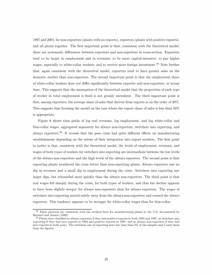
that, among exporters, the average share of sales that derives from exports is on the order of 20%.

This suggests that focusing the model on the case where the export share of sales is less than 50%

is appropriate.

Figure 6 shows time paths of log real revenues, log employment, and log white-collar and

blue-collar wages, aggregated separately for always non-exporters, switchers into exporting, and

always exporters.39 It reveals that the peso crisis had quite different effects on manufacturing

establishments depending on the extent of their integration into export markets. The first point

to notice is that, consistent with the theoretical model, the levels of employment, revenues, and

wages of both types of workers for switchers into exporting are intermediate between the low levels

of the always non-exporters and the high levels of the always exporters. The second point is that

exporting plants weathered the crisis better than non-exporting plants. Always exporters saw no

dip in revenues and a small dip in employment during the crisis. Switchers into exporting saw

larger dips, but rebounded more quickly than the always non-exporters. The third point is that

real wages fell sharply during the crisis, for both types of workers, and that the decline appears

to have been slightly steeper for always non-exporters than for always exporters. The wages of

switchers into exporting moved subtly away from the always non-exporters and toward the always

exporters. This tendency appears to be stronger for white-collar wages than for blue-collar.

38 These patterns are consistent with the stylized facts for manufacturing plants in the U.S. documented byBernard and Jensen (1999).

39 Plants were classified as always exporters if they had positive exports in both 1993 and 1997, as switchers intoexporting if they had zero exports in 1993 and positive exports in 1997, and as always non-exporters if they hadzero exports in both years. The switchers out of exporting were few (less than 5% of the sample) and I omit themfrom the figures.

25

4.2 Econometric Strategy

Although such descriptive comparisons of means across plants with different export status are

suggestive, they can also be misleading. Differences between exporters and non-exporters in cross-

section may simply be due to selection of more-productive (higher-λ) plants into the export market,

and changes between always non-exporters, switchers, and always exporters over time may reflect

changing patterns of selection based on shocks to productivity over time. This section presents

an econometric strategy that is not confounded by such endogenous selection. The strategy is

based on a comparison of within-plant changes over time between plants distinguished by their

underlying productivity prior to the crisis, rather than by the choices they make in response to

the crisis.

The first econometric task is to find a proxy for the unobserved parameter, λ. The theoretical

model suggests that a number of different observable variables – wages, the wage ratio, the capital-

labor ratio, total employment, total sales, the export share of sales – are related to λ. But the

problem of inferring λ is complicated by the fact that the observable variables that are weighted

averages of the two production lines depend on λ in two ways: through the plant’s decisions on

each line and through the export share of output. My primary strategy for avoiding this difficulty

is to use as a proxy the one observable variable that is both non-zero for the all plants in the

dataset and observable at the production-line level: domestic sales. The model suggests that

in cross-section domestic sales will be a smooth, continuous, monotonically increasing function

of the know-how parameter λ. Appendix A.10 shows that, using a first-order approximation,

λ − λ = 1B

(ln (Sss)− ln (Sss)

)where λ and ln (Sss) are industry means, and B is a positive

constant that depends on the industry-average productivity but not on the productivity of a

particular plant. Up to a scaling factor, the deviated log of domestic sales can thus be taken

directly as a proxy for (deviated within industry) know-how.

Alternatively, a simple and transparent method for combining the information from the several

variables that the model suggests are correlated with λ into a single index is to take their first

principal component, the single linear combination of the several variables that best accounts for

the variance in their joint distribution.40 As a robustness check, I estimate the same econometric

model using this proxy for λ. The variables included in the principal component calculation are

40 Another approach would be to use the multiple-indicator multiple-cause framework of Goldberger (1972,1974), and use factor-analytic techniques to make more efficient use of the information available in the variousplant characteristics. This approach is unattractive for present purposes because it depends on a number ofrestrictive assumptions on the disturbance terms in the equations relating the indicators to the unobserved factor,assumptions that are unlikely to hold in a dataset as rife with measurement error as a plant-level panel from adeveloping country. The factor-analysis approach may still be promising, however, and it remains a subject forfuture work.

26

total employment, total revenues, the export share of sales, the capital labor ratio, wage level for

each type of worker, and the employment ratio (the ratio of white-collar to blue-collar employ-

ment). I also include an indicator for whether the plant has received foreign direct investment.

While this variable does not enter into the theoretical model, it seems plausible that foreign-owned

plants have greater access to the knowledge and technologies of their parent companies, and hence

that foreign ownership is an indicator for unobserved know-how.

Once I have estimated the proxy, the remainder of the estimation procedure is straightforward.

I simply regress within-plant changes in plant characteristics on the proxy dummies for the 205

6-digit industries and 32 states in Mexico. Let λ be the estimate for λ from before the crisis. The

model can be written:

dyj = λj · β + Dj · γ + εj (25)

where j indexes plants, Dj is a vector of indicators for industry and state within Mexico, εj

is a mean-zero disturbance, assumed to be uncorrelated with λj, and dyj is a within-plant change

in one of the set of plant characteristics that the model suggests should be affected by quality

upgrading. The parameter of interest in this equation is β. Identification of β is based implicitly

on a comparison of within-plant changes over the crisis years between initially high-λ and low-λ

plants.41 A significant positive coefficient can be interpreted as evidence of differential upgrading

within industries.

This specification presumes that no omitted variables are correlated with both λj and dyj.

A possible concern is that plants’ underlying know-how itself changes over time, and that the

changes are correlated with its initial level. This would be the case, for instance, if plants near the

technological frontier are better able to learn about new technological advancements. I address

this possibility by re-estimating the same econometric model in different periods. If a positive

coefficient on λj for the peso crisis years were due to a process of non-uniform technical diffusion

rather than the exchange rate shock, then we would expect to find a similar coefficient on λj in

periods during which a major exchange-rate shock did not intervene.

41 This estimation strategy can also be interpreted in an instrumental-variables framework. The know-how proxycan be thought of as an instrument for the change in exports during the crisis, which might then be used to estimatethe effect of exporting on plant-level behavior. The danger with this interpretation is that it is not clear what itmeans to talk about a causal effect of exporting on plant behavior: a plant’s decision to enter the export marketand its decision to upgrade quality can both be interpreted as manifestations of the plant’s solution to a singleunderlying optimization problem. But if we think of the estimation strategy as investigating the reduced-formrelationship between initial level of productivity and both the change in exports and the average quality of goodsproduced, then this danger is avoided and the interpretation is clear. This interpretation underlines the similarityof this approach to that of Chay and Greenstone (2001), who use initial levels of air pollution as an instrument forchanges in pollution at the country level in response to the 1981-1982 recession in the U.S.

27

A second concern with this specification is that it regresses changes on levels, and mean

reversion due to measurement error may bias the coefficient estimates. This issue is not relevant

to the main estimates of the paper, which regress changes in wages and the wage ratio on the

initial level of domestic sales. But it may be important for regressions involving changes in sales,

changes in the export share of sales (in which domestic sales enters in the denominator), or possibly

changes in total employment (for reasons explained below), as well as for regressions using the

first principal component. To deal with this issue, when using log domestic sales, I present both

OLS results and IV results, instrumenting the initial level of domestic sales with sales from the

previous year. When using the first principal component, I leave out of the principal component

estimation the variable that appears in changes on the left hand side of the subsequent regression.

4.3 Basic Results

Let us begin with a set of graphs that illustrate the main results. Figures 7a-7d plots locally

smoothed non-parametric regression lines of the levels of the export share, white-collar and blue-

collar wages, and the wage ratio in pre- and post-crisis years against log domestic sales in 1993.

The dark, bold curves are for the pre-crisis year, the gray curves for the post-crisis year. All

variables have been deviated from year-specific industry means; hence the relevant information is

contained in the slopes of the curves, not the levels. To avoid the issue of mean reversion, Figure

7a plots the export percentage of sales in 1994 instead of 1993, as well as in 1997. The figure

reveals (1) that in cross-section higher-λ have higher export shares, and (2) that there was a larger

increase in the export share in plants with higher domestic sales in 1993.42 Figures 7b-7d plot

similar graphs for white-collar wages, blue-collar wages, and the wage ratio in 1993 and 1997. In

cross-section, wages for both types of workers and the wage ratio are increasing in λ (log domestic

sales). The changes in the slopes of the curves between 1993 and 1997 are subtler than for the

export share, but still evident: higher-λ plants saw greater increases in these wage variables than

lower-λ plants from 1993-1997. It appears that the increase in slope was greater for white-collar

than for blue-collar wages, and the fact that the slope of the wage ratio curve also increased

confirms this.

As argued above, if the relationship between initial productivity and the changes in wages and

capital intensity were due to an omitted variable unrelated to the peso crisis, then we would expect

to see the same relationship showing up in other periods in which there was no such shock. To

42 The spikes at the left ends of both curves are due to a small number of plants with very low domestic salesand high exports. These plants appear to be maquiladoras that were included in the EIA dataset by mistake (andthat my cleaning procedures have failed to filter out because they report non-zero domestic sales.)

28

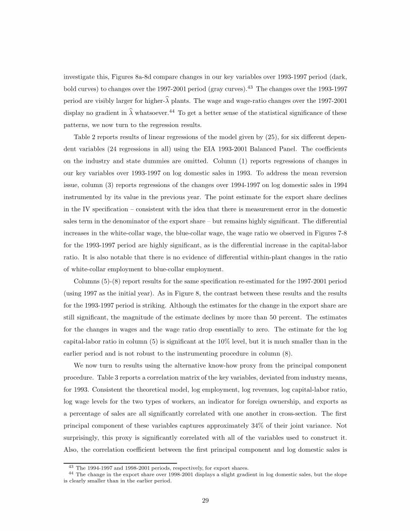
investigate this, Figures 8a-8d compare changes in our key variables over 1993-1997 period (dark,

bold curves) to changes over the 1997-2001 period (gray curves).43 The changes over the 1993-1997

period are visibly larger for higher-λ plants. The wage and wage-ratio changes over the 1997-2001

display no gradient in λ whatsoever.44 To get a better sense of the statistical significance of these

patterns, we now turn to the regression results.

Table 2 reports results of linear regressions of the model given by (25), for six different depen-

dent variables (24 regressions in all) using the EIA 1993-2001 Balanced Panel. The coefficients

on the industry and state dummies are omitted. Column (1) reports regressions of changes in

our key variables over 1993-1997 on log domestic sales in 1993. To address the mean reversion

issue, column (3) reports regressions of the changes over 1994-1997 on log domestic sales in 1994

instrumented by its value in the previous year. The point estimate for the export share declines

in the IV specification – consistent with the idea that there is measurement error in the domestic

sales term in the denominator of the export share – but remains highly significant. The differential

increases in the white-collar wage, the blue-collar wage, the wage ratio we observed in Figures 7-8

for the 1993-1997 period are highly significant, as is the differential increase in the capital-labor

ratio. It is also notable that there is no evidence of differential within-plant changes in the ratio

of white-collar employment to blue-collar employment.

Columns (5)-(8) report results for the same specification re-estimated for the 1997-2001 period

(using 1997 as the initial year). As in Figure 8, the contrast between these results and the results

for the 1993-1997 period is striking. Although the estimates for the change in the export share are

still significant, the magnitude of the estimate declines by more than 50 percent. The estimates

for the changes in wages and the wage ratio drop essentially to zero. The estimate for the log

capital-labor ratio in column (5) is significant at the 10% level, but it is much smaller than in the

earlier period and is not robust to the instrumenting procedure in column (8).

We now turn to results using the alternative know-how proxy from the principal component

procedure. Table 3 reports a correlation matrix of the key variables, deviated from industry means,

for 1993. Consistent the theoretical model, log employment, log revenues, log capital-labor ratio,

log wage levels for the two types of workers, an indicator for foreign ownership, and exports as

a percentage of sales are all significantly correlated with one another in cross-section. The first

principal component of these variables captures approximately 34% of their joint variance. Not

surprisingly, this proxy is significantly correlated with all of the variables used to construct it.

Also, the correlation coefficient between the first principal component and log domestic sales is

43 The 1994-1997 and 1998-2001 periods, respectively, for export shares.44 The change in the export share over 1998-2001 displays a slight gradient in log domestic sales, but the slope

is clearly smaller than in the earlier period.

29

.81, which supports the assertion that the two indexes are capturing a similar underlying pattern

in the cross-sectional data. Table 4 reports results similar to those in Table 2 columns (1)-(2)

and (5)-(6), but using the first principal component as the productivity proxy.45 The qualitative

pattern of results is identical to that of Table 2.

Table 5 reports results using both proxies for changes in log total revenues and log total

employment. Two caveats are important. The first is that the theoretical model did not generate

a strong implication for the relationship between changes in these variables and the initial level of

the productivity parameter λ. Firms with greater know-how firms see a larger increase in exports

but also a larger decrease in domestic sales; the net effect is ambiguous. The second is that the

EIA panel is beset by two somewhat unusual forms of measurement error related to the reporting

patterns of multi-establishment firms.46 On one hand, some self-contained production complexes

operated by a single firm are divided into several establishments for the purposes of responding to

the survey. Moving one stage of the production process from one building to the next will show

up in the data as a spurious increase in both employment and sales in one establishment and

a spurious decrease in another. On the other hand, the EIA survey allows multi-establishment

firms to report information for more than one establishment on a single questionnaire, but INEGI

did not keep track of these reporting patterns in a systematic way before 1998. Unobserved

changes in the pattern of reporting would have similar consequences in the data to the shifting of

production lines between buildings. Both of these peculiarities generate measurement error that

is highly correlated between sales and employment, and also correlated over time. This form of

measurement error may be part of the explanation for the sharp contrast between results for the

changes in log employment and log revenues using the two different productivity proxies. In the

1993-1997 period, we see that the estimates are close to zero and insignificant when using log

domestic sales, even instrumenting domestic sales in 1994 with the previous year, and positive

and highly significant when using the first principal component. It is possible that the correlated

measurement error between domestic sales and employment is biasing the estimates downward, and

that the persistence of the measurement over time is such that instrumenting with a previous year

does not remove the error. The fact that the results differ to such an extent under the principal-

component approach lend credence to this view. It is also possible, however, that changes in

revenues and employment were not in fact larger in initially more-productive plants. These results

should be interpreted with caution.

45 Recall that the productivity proxy differs slightly across regressions, since the variable entered in changes onthe left-hand side is omitted from the principal component calculation.

46 Unfortunately, the EIA survey does not report whether or not a plant is part of a multi-establishment firm,and a natural test – to re-estimate the model only with single establishment firms – is unavailable.

30

We now turn to the EIA 1984-2001 Balanced Panel, in order to compare the 1993-1997 period

to earlier periods as well. I re-estimate the basic model for four periods: 1986-1989,47 1989-1993,

1993-1997 and 1997-2001. Table 6 reports the results for the same model as in Table 2, columns

(1)-(2) for these four periods. The results for 1993-1997 and 1997-2001 are consistent with the

results in Table 2. The estimates for the 1989-1993 resemble those for the 1997-2001 period.

We see no evidence of differential upgrading in wages or the wage ratio. The only variable for

which we have a result that might be interpreted as evidence of upgrading is the capital-labor

ratio. In 1986-1989, by contrast, there is evidence of a larger increase in the white-collar wage

among initially more productive plants. It is notable that 1986 was also a year in which the

peso depreciated markedly (as can be seen in Figure 2a above), losing 46% of its value over the

course of the year.48 The results for 1986-1989 can be seen as providing additional support for the

hypothesis of differential quality upgrading induced by exchange rate movements.49

The one coefficient estimate in Table 6 that is out of line with the results from tables 2 and 4

is the significant coefficient for the employment ratio in 1993-1997. This finding does not appear

to be robust, however. Table 7 reports results analogous to Table 6, but using the first principal

component as the productivity proxy. The results are quite similar to those of Table 6, except

that the estimate for the employment ratio in 1993-1997 is no longer significant.50

The estimates above have been based on balanced panels from which plants that went out of

business have been removed completely. Selection bias is a possible concern. In order to test for

this possibility, I estimate my basic model using the EIA 1993-2001 Unbalanced Panel and the

standard two-step selection correction method (Heckman, 1976).51 Table 8 reports the results

for the 1993-1997 and for the 1997-2001 periods. The first-stage coefficient on initial-year log

domestic sales is positive and highly significant, as the theoretical model would lead us to expect.

The results for the export percentage, wages, the wage ratio, the capital-labor ratio, and the

employment ratio are in line with the results for Table 2, which we have already discussed. We

47 The choice of 1986 as the initial year is dictated by the lack of data on exports in 1984-1985.48 This occurred through ongoing market pressures and adjustments of the exchange rate targets, rather than a

single discrete shock.49 One reason that the effects may be weaker in this period than the 1993-1997 period is that Mexican firms in

the early stages of liberalization had little knowledge or experience with exporting. Although the number of plantswith some exports in the EIA 1984-2001 Balanced Panel rose from 22% to 33% over the period, the plants werenot successful at selling large volumes of goods. The export share of total output in the panel rose from 5% to just8% over the same period.

50 I do not report a separate table results using the IV method of Table 2 columns (3)-(4). Results were similarto those in Table 6.

51 I do not have instruments that affect only the probability of remaining in the sample and not my otheroutcome variables. The coefficient on the inverse Mills’ ratio term in the second stage is thus identified only bythe assumption of bivariate normality of the first and second stage errors. Nevertheless, the selection-correctedestimates may have diagnostic value: if the results were significantly different from the results for balanced panelsreported above, we would have cause for concern.

31

can simply note again that the estimates for the changes in wages and in the wage ratio in the

1993-1997 period, as well as the contrast between results for the 1993-1997 and 1997-2001 period,

are quite robust.

4.4 Additional Findings

In this sub-section, I discuss additional findings from the Encuesta Nacional de Empleo, Salarios,

Tecnologia y Capacitacion (ENESTyC) [National Survey of Employment, Wages, Technology and

Training], a special survey carried out by INEGI in 1992, 1995 and 1999. Although the ENESTyC

has not followed individual plants over time as closely as the EIA and EIM, and consequently

appears to contain more measurement error, it has two advantages: first, it collected information

on a wider range of plant characteristics; and second, it contains information on the maquiladora

sector. Details on the sampling design and variable definitions appear in the data appendix.

I use the ENESTyC data to address three issues. The first is whether changes in the wider

range of plant characteristics we observe are consistent with the hypothesis of differential quality

upgrading. The second is whether we can use the wider range of plant characteristics to distinguish

between the alternative interpretations of the increases in wages within occupational categories

set out in the theoretical part above: whether the wage changes reflect changes in the sorting

of heterogeneous workers into plants, changes in training programs, or changes in wage premia

offered for efficiency-wage reasons. The third is to what extent Feenstra and Hanson’s outsourcing

hypothesis is consistent with the information in this newly available dataset.

Table 9 reports means and standard deviations for relevant variables from the ENESTyC

in the three waves of the survey, separately for maquiladoras, non-maquila non-exporters, and

non-maquila exporters. To begin, I consider only the differences between exporters and non-

exporters in the non-maquiladora sector, and return to the maquiladora sector when discussing

the Feenstra-Hanson model below. The most relevant variable for this paper is the indicator

of ISO 9000 certification, an international production standard certified by independent local

certifying agencies.52 We see that in cross-section, exporters are more likely than non-exporters

to have the certification in 1995, and the difference increases in 1998. We also see that exporters

have higher average schooling among white-collar workers and blue-collar workers, lower absentee

rates, a higher likelihood of providing formal training, and a lower fraction of manual (as opposed

52 The ISO 9000 group of industry-specific standardsmainly concern management and documentationprocedures,rather than the quality of output, but the common view among managers in Mexico is that ISO certification alsosignals high product quality. ISO certification is not cheap talk. The process of obtaining certification is time-consuming and expensive - typically taking between nine months and two years, and costing on average $187,000(1996 U.S. dollars) (Guler et al, 2002).

32

to electronic or numerically controlled) equipment.53 As in the EIA data, exporters on average

employ more workers and pay higher wages to both types of workers, but especially to white-

collar workers, but employ roughly the same ratio of white- to blue-collar workers in production.

Somewhat surprisingly, exporters also have a higher reported accident rate and a higher turnover

rate.54

We now turn to the question of whether the changes in these variables over time are consistent

with the differential quality upgrading hypothesis. I estimate the same econometric model as

used with the EIA data above. Because the information from the EIA on domestic sales is more

reliable than in the ENESTyC, I focus on the plants that appear in both datasets and use the

EIA information. (See the data appendix for details on the linked panels.) Table 10 reports the

results, using log domestic sales as the know-how proxy. The strongest result is for the ISO 9000

certification indicator. The magnitude suggests that a doubling of domestic sales in the initial

year would lead to an increase in the likelihood of acquiring the certification of 8%. Although

I do not have access to data on changes in ISO certification for other periods,55 and hence am

not able to construct an estimate of what would have happened in the absence of the peso crisis,

this result appears to provide fairly strong corroborating evidence that plants with initially larger

domestic sales did in fact improve their quality levels.

The remaining results for the 1994-1998 period do not provide evidence of changes in plant

behavior. The estimates for the changes in whether the plant has a formal training program, the

accident rate, the absentee rate, and the turnover rate are statistically indistinguishable from zero

and imprecisely estimated. If we believe that higher efficiency wages should be accompanied by

less absenteeism and lower turnover, then these results may be interpreted as evidence against the

efficiency-wage hypothesis and in favor of the hypothesis that quality upgrading requires hiring

workers of higher inherent skill. It is also possible, however, that the non-results for these variables

are due to the fact that they are extremely poorly measured, and carry little signal of the true

behavior of the plant.

The data from the 1992 and 1999 waves of the ENESTyC (but not the 1995 wave) include data

on average schooling by occupational category. These data also bear on the sorting vs. efficiency

wage issue. If increasing observed wages only reflected rising efficiency wages, we would not expect

53 Note that the table reports standard deviations of the data, not standard errors of the means. These differencesare all highly statistically significant.

54 Note that the overall averages for several of these variables, especially the absentee rate, the accident rate andthe turnover rate, appear to be quite volatile across waves, which most likely arise from subtle differences in thewording of questions in the different questionnaires. This suggests that the results for these variables should beinterpreted with caution.

55 The ENESTyC was carried out again in 2001, and has recently become available. I hope in the future to gainaccess to the data, and to be able to compare changes over the 1998-2000 period with earlier changes.

33

to see evidence of rising average schooling within occupational category. The results, reported in

Columns (3) and (4) of Table 10, are mixed. The initial level of log domestic sales is significantly

related to the change in average schooling of blue-collar workers. Somewhat surprisingly, the

coefficient for the average schooling of white-collar workers, while positive, is markedly smaller

than that for blue-collar workers and not significant. Given the finding from the EIA that the

relative wage of white-collar workers rose more in firms with greater domestic sales, these findings

suggest that efficiency wages may be more important for white-collar than blue-collar workers. It

is worth emphasizing again, however, that the sample sizes are small, the data are noisy, and we

do not have a counterfactual comparison of what would have happened in the absence of the peso

crisis. These results should be seen as suggestive rather than definitive.

Finally, we are in a position to re-evaluate the outsourcing hypothesis mentioned in the in-

troduction in the light of these micro-datasets which were not available to Feenstra and Hanson.

This paper has presented evidence that the peso crisis induced differential changes in wages within

industries, but not differential changes in the proportion of white- and blue-collar workers in pro-

duction. The wage changes thus appear not to be explained by a demand shift toward greater

numbers of white-collar workers. A defense of the outsourcing hypothesis would be to argue that

the results in this paper are focused on the non-maquiladora sector, that outsourcing is likely to

be more important in the maquiladora sector, and that the rapid growth of the maquiladora sector

following the peso crisis may still have been responsible for the aggregate increase in inequality.

But Table 9 shows that maquiladoras employ a greater proportion of blue-collar workers – and

that the blue-collar workers that they employ have less education on average – than either ex-

porters or non-exporters in the rest of the manufacturing sector.56 These facts suggest that the

first-order consequence of the growth of the maquiladora sector in Mexico was an increase in the

relative demand for low-skilled workers.

5 Conclusion

This paper has set out a new model that links expanding trade and increasing inequality through

the mechanism of differential quality upgrading within industries. The paper has also presented a

new empirical approach, derived directly from the theoretical framework, that uses the exchange

rate shock of the late-1994 peso crisis to evaluate the implications of the theoretical model. I

find robust evidence of differential quality upgrading in the 1993-1997 period and essentially no

56 This observation is due originally to Pablo Ibarraran (2003). In unreported results, I find that these patternshold true even once we control for industry and region effects.

34

evidence in the 1989-1993 and 1997-2001 periods. These results strongly support the quality-

upgrading hypothesis.

A number of questions remain outstanding. One is to what extent the quality-upgrading

hypothesis can explain changes in inequality at the aggregate level in Mexico. There are three

channels through which differential quality upgrading within industries may contribute to ag-

gregate wage inequality. First, it raises wage dispersion within occupational categories between

less-productive and more-productive plants. Second, it may lead to a re-allocation of production

toward more-productive plants, which are more unequal than less-productive plants. Third, it

generates an increase in wage inequality within the plants that upgrade. Together these channels

may account for aggregate within-industry increases in wage inequality that more than offset the

between-industry shifts toward industries intensive in unskilled labor illustrated by Figure 1 in

the introduction. To what extent they do so is a topic for future work.

A second outstanding question is the generalizability of the quality-upgrading hypothesis.

The empirical analysis in this paper is specific to a particular historical event with particular

characteristics. Nonetheless, there are reasons to believe that differential quality upgrading may

occur in response to other trade-related shocks. We would expect a bilateral reduction in tariffs,

transport costs or fixed costs of exporting to have an effect similar to an exchange-rate shock on

firms in a country like Mexico: the incentive to export increases and domestic sales decrease (here

because of an increase in import competition rather than a contraction of domestic demand) and

differential quality upgrading generates an increase in the relative wage of white-collar workers.57

If this is the case, the quality upgrading hypothesis is likely to be a part of the explanation of the

link between trade liberalization and wage inequality more generally.

Final judgment on this issue must await more empirical work, in other countries, responding

to other shocks. But if the quality-upgrading hypothesis stands up, then it may help to resolve a

second, related puzzle in the political economy of trade policy. The simplest Hecksher-Ohlin model

predicts that in developing countries unskilled workers will be winners and skilled workers and

owners of capital losers from international integration. From this perspective, it is a mystery why

in many developing countries, especially in Latin America, the biggest proponents of integration

are educated, urban elites. This paper has also identified winners and losers from trade, but

along a different dimension. The winners are the entrepreneurs and employees, especially the

white-collar employees, with either the qualifications or the good fortune to be employed in the

most modern, technically sophisticated, internationally oriented plants within each industry. The

losers are people, especially the unskilled, in less-productive, domestically oriented plants. In this

57 An appendix that works out the formal logic of this argument is available from the author.

35

view, both the enthusiasm of the most educated and the pessimism of the poorest and least skilled

toward globalization may make economic sense.

36

Appendix A: Theory Appendix

A.1: Micro-Foundations of Aggregate Demands

Following Andersen et al (1992)’s extension of McFadden (1978, 1981), we assume the randommatch-specific term εij in (1) has c.d.f. F (ε) = exp

(− exp

(− ε

µ + γ))

, where γ = .5772 (Euler’sconstant) is included to ensure that the expectation of εij is zero, and µ is a positive constant.The probability that consumer i chooses variety j, call it P ij can be derived as follows:

P ij = Pr(εi1, εi2, ...εiJ |Vij > Vit, ∀t 6= j)= Pr(εit < θqj − pj − (θqt − pt) + εij, ∀t 6= j)

Because the ε′s are i.i.d., the probability that variety j is chosen conditional on a particularvalue of εij , is the product of the c.d.f.s:

P ij|εij =∏t 6=j

F (θqj − pj − (θqt − pt) + εij)

The marginal probability is the expected value of the conditional probability over all εij :

P ij =

∞∫−∞

∏t 6=j

F (θqj − pj − (θqt − pt) + ε)

f(ε)dε

=

∞∫−∞

∏t 6=j

exp[− exp

(−θqj − pj − (θqt − pt) + ε

µ+ γ

)] f(ε)dε

The p.d.f. of the distribution of εij is given by:

f (ε) =1µ

exp(− ε

µ+ γ

)exp

[− exp

(− ε

µ+ γ

)]Let φ ≡ exp

(− ε

µ + γ). Then dφ = − 1

µ exp(− ε

µ + γ)

dε.The marginal probability can then be written:

P ij = −0∫∞

exp (−φ)∏t 6=j

exp [−φ exp (− [θqj − pj − (θqt − pt)] /µ)] dφ

= −0∫∞

exp (−φ) exp

−φ exp [− (θqj − pj) /µ]∑t 6=j

exp [(θqt − pt) /µ]

dφ

= −0∫∞

exp

−φ

1 + exp [− (θqj − pj) /µ]∑t 6=j

exp [(θqt − pt) /µ]

dφ

37

= −0∫∞

exp

−φ

J∑

t=1exp [(θqt − pt) /µ]

exp [(θqj − pj) /µ]

dφ

=exp [(θqj − pj) /µ]

J∑t=1

exp [(θqt − pt) /µ]

The expected aggregate demand for variety j, for all N consumers, is then:

E (xj) = N · P ij =N exp [(θqj − pj) /µ]J∑

t=1exp [(θqt − pt) /µ]

A.2: Wage Ratios

From (9), we have: wh∗ (λ) = wh + αhθq∗ (λ) and wl∗ (λ) = wl + αlθq∗ (λ), where q∗ (λ) =(ηλθα)1/1−α. Making the dependence of the wage and quality terms on λ implicit to reduceclutter:

∂(wh∗/wl∗)

∂λ=

(∂wh∗/∂λ

)wl + αlθq∗

− (∂wl∗/∂λ

) wh + αhθq∗

wl∗2

=θq∗

(1−α)λ

αhwl − αlwh

wl∗2

The numerator will be positive, and∂(wh∗/wl∗)

∂λ > 0 if and only if αh/αl > wh/wl.Similarly:

∂(wh∗/wl∗)

∂θ=

(∂wh∗/∂θ

)wl + αlθq∗

− (∂wl∗/∂θ

) wh + αhθq∗

wl∗2

=q∗

(1−α)

αhwl − αlwh

wl∗2

Again, the numerator will be positive and∂(wh∗/wl∗)

∂θ > 0 if and only if αh/αl > wkh/wk

l .

A.3: Export Share of Output vs. Know-how Parameter

From (18):

∂x∗cd (λ)∂λ

=∂I∗cd

∂λxcd (26)

= (ηδαcdλ

αθd)1/1−α

x∗cd (λ)

38

conditional on the firm entering consumer market d. From the definition of χ∗s (λ), we have:

∂χ∗s (λ)∂λ

=(x∗ss (λ) + x∗sn (λ)) ∂x∗sn(λ)

∂λ − x∗sn (λ)(

∂x∗ss(λ)∂λ + ∂x∗sn(λ)

∂λ

)(x∗ss (λ) + x∗sn (λ))2

=x∗ss (λ)x∗sn (λ)

(∂I∗sn(λ)

∂λ − ∂I∗ss(λ)∂λ

)(x∗ss (λ) + x∗sn (λ))2

= χ∗s (λ) (1− χ∗s (λ)) (ηδαcdλ

α)1/1−α

θ1/1−αn − θ1/1−α

s

> 0

for all λ > 0, since θn > θs by assumption.

A.4: Export Share of Sales vs. Know-how Parameter

Noting that S∗ss (λ) = p∗ss (λ)x∗ss (λ) and S∗sn (λ) = p∗sn (λ)x∗sn (λ), take the partial derivativeof both sides of the definition of σs (λ) with respect to λ. (For notational convenience, I drop theexplicit dependence of pss, psn, xss and xsn on λ.)

∂σs

∂λ= σs (λ) (1− σs (λ))

[∂xsn

∂λ

xsn−

∂xss

∂λ

xss

]+

[∂psn

∂λ

psn−

∂pss

∂λ

pss

](27)

From (26) in Appendix A.3 we have that

∂xsd

∂λ= [ηθd (λδsd)

α]1/1−αxsd

Simplifying the first term in square brackets in (27), we have:[∂xsn

∂λ

xsn−

∂xss

∂λ

xss

]= ηλα/1−α

[(θnδα

sn)1/1−α − (θs)1/1−α

]> 0 (28)

Since θn > θs and δsn ≥ 1.From (18), we have that

∂psd

∂λ= αδsdθd

∂qsd

∂λ=

αδsdθdqsd

(1− α)λ

Simplifying the second term in square brackets in (27), we have:[∂psn

∂λ

psn−

∂pss

∂λ

pss

]=

α

(1− α)λ

[δsnθnqsn

psn− δssθsqss

pss

]Substituting for psn and pss from (18) and defining φ ≡ µ + wh

s + wls, the term in brackets on

the right hand side can be re-written:

δsnθnqsn

psn− δssθsqss

pss=

1psnpss

δsnθnqsn

[µ + wh

s + wls + αθsqss

] − (29)

1psnpss

θsqss

[µ + wh

s + wls + αδsnθnqsn

]

39

=1

psnpss

(µ + wh

s + wls

)(δsnθnqsn − θsqss) > 0

From (27), (28) and (29), we can conclude that ∂σs/∂λ > 0.

A.5: Comparative-Static Results for Entry

The zero-profit conditions determining entry (20) can be rewritten:

D∗s

(λmin

ss , λminns

)=

µNs

fssexp

I∗ss

(λmin

ss

)(30)

D∗s

(λmin

ss , λminns

)=

µNs

fnsexp

I∗ns

(λmin

ns

)(31)

D∗n

(λmin

sn , λminnn

)=

µNn

fsnexp

I∗sn

(λmin

sn

)(32)

D∗n

(λmin

sn , λminnn

)=

µNn

fnnexp

I∗nn

(λmin

nn

)(33)

Consider first the effect of the devaluation of the peso. Taking the derivative of both sides of(30) and (31) with respect to δsn and solving for ∂λmin

ss /∂δsn, we have:

∂λminss

∂δsn=

1Ωs

∂I∗ns

(λmin

ns

)∂λmin

ns

[∂D∗

s

∂δsn

]+

∂D∗s

∂λminns

∂I∗ss

(λmin

ss

)∂δsn

−∂I∗ns

(λmin

ns

)∂δsn

(34)

where

Ωs ≡ D∗s

∂I∗ss

(λmin

ss

)∂λmin

ss

∂I∗ns

(λmin

ns

)∂λmin

ns

− ∂D∗s

∂λminss

∂I∗ns

(λmin

ns

)∂λmin

ns

− ∂D∗s

∂λminns

∂I∗sd

(λmin

ss

)∂λmin

ss

> 0 (35)

It follows from the definition of I∗cd

(λmin

cd

)that ∂I∗ss

(λmin

ss

)/∂δsn = 0 and ∂I∗ns

(λmin

ns

)/∂λmin

ns >

0. Since δns ≡ 1/δsn, we also have that ∂I∗ns

(λmin

ns

)/∂δsn < 0. From (16) and (17), we have that

∂D∗s/∂λmin

ns < 0. Note further that:

∂D∗s

∂δsn=

∫ λmaxs

λminsd

∂I∗ns (λ)∂δsn

exp I∗ns (λ)Msgs (λ) dλ < 0

Given these relationships, we can conclude from (34) that ∂λminss /∂δsn < 0.

To sign ∂λminsn /∂δsn, we simply take the derivative of both sides of (32). The assumption

that aggregate supply to the Northern market is approximately unaffected by the peso crisis isequivalent to assuming that the aggregate quantity D∗

n is unchanged. Thus we have:

µNn

fsnexp

I∗sn

(λmin

sn

)∂I∗sn

(λmin

sn

)∂λmin

sn

∂λminsn

∂δsn+

∂I∗sn

(λmin

sn

)∂δsn

= 0

40

which yields:

∂λminsn

∂δsn= −

∂I∗sn(λminsn )

∂δsn

∂I∗sn(λminsn )

∂λminsn

It follows again from the definition of I∗cd (·) that ∂I∗sn

(λmin

sn

)/∂δsn > 0 and ∂I∗sn

(λmin

sn

)/∂λmin

sn >

0. Thus ∂λminsn /∂δsn < 0.

Now consider the effect of the reduction in the number of consumers in South. Note that D∗s

and I∗cs

(λmin

cs

)do not depend directly on Ns; they are affected only through λmin

ss and λminns . Hence

taking the derivative of both sides of (30) and (31) with respect to Ns and solving for ∂λminss /∂Ns,

we have:

∂λminss

∂Ns= −

∂I∗ns

(λmin

ns

)∂λmin

ns

(D∗

s

ΩsNs

)(36)

where Ωs is defined as in (35) above. Since ∂I∗ns

(λmin

ns

)/∂λmin

ns > 0 by the definition of I∗cd (·)in (19), it follows that ∂λmin

ss /∂Ns < 0. Finally, since no other terms in (32) depend on Ns itfollows immediately that λmin

ss does not depend on Ns, that is, ∂λminsn /∂Ns = 0.

Finally, we state precisely the condition required to ensure that the exchange-rate shock inducesexit of Southern firms from the Southern market. The net effect of the shock on the cut-off fordomestic firms to enter the Southern market is:

dλminss =

∂λminss

∂δsndδsn +

∂λminss

∂NsdNs

Given our results for ∂λminss /∂δsn and ∂λmin

ss /∂Ns in (34) and (36) above, dλminss > 0 (and the

exchange-rate shock induces exit of Southern firms from the Southern market) if and only if:

−dNs

dδsn>

− ∂D∗s

∂δsn+

∂D∗s

∂λminns

· ∂I∗sn(λminns )

∂δsn

∂I∗sn(λminns )

∂λminns

Ns

D∗s

(37)

We will maintain this assumption in what follows.

A.6: Changes in Firm-level Observables

Note that the total effect of the exchange rate shock on output on each production line can beexpressed as:

dxsd (λ) =∂xsd (λ)

∂δsndδsn +

∂xsd (λ)∂Ns

dNs (38)

for d = s, n. Recall from (18) that

x∗sd (λ) =Nd

D∗d

exp I∗sd (λ) (39)

Consider first the effect on output on the domestic production line, xss. Taking the partialderivative of both sides of (39) with respect to δsn, and noting that I∗ss (λ) does not depend onδsn, we have:

41

∂xss (λ)∂δsn

= − Ns

(D∗s )2

exp I∗ss (λ) ∂D∗s

∂δsn> 0

since ∂D∗s/∂δsn < 0. Taking the partial derivative of both sides of (39) with respect to Ns, we

have:

∂xss (λ)∂Ns

=1

D∗s

exp I∗ss (λ) > 0

Substituting these into (38), we have:

dxss (λ) =exp I∗ss (λ)

D∗s

−Ns

D∗s

∂D∗s

∂δsndδsn + dNs

(40)

= xss (λ)− 1

D∗s

∂D∗s

∂δsndδsn +

1Ns

dNs

If the condition required to ensure that the exchange-rate shock induced exit of Southern firms

from the domestic market (equation (37) in Appendix A.5) is satisfied, then the term in curlybraces will be negative. Thus in the empirically relevant case, dxss (λ) < 0.

Now consider the effect on the output of the export production line. Taking the partial of bothsides of (39) with respect to δsn, recalling the assumption that the aggregate D∗

n is approximatelyunaffected by the changes in exports of Southern firms, we have:

∂xsn (λ)∂δsn

=Nn

D∗n

exp I∗sn (λ) ∂I∗sn (λ)∂δsn

> 0

since ∂I∗sn (λ) /∂δsn > 0 by (19). Because of the segmentation of consumer markets, the changein the number of Southern consumers does not affect output of Southern firms for the Northernmarket. The only change in output for export is the change induced by the change in the exchangerate. Hence:

dxsn (λ) =Nn

D∗n

exp I∗sn (λ) ∂I∗sn (λ)∂δsn

dδsn (41)

= xsn (λ)∂I∗sn (λ)

∂δsndδsn

Hence we know dxsn (λ) > 0.

Now consider the change in the export share of output for Southern firms in case (5) above,the always exporters. Recall that χs (λ) ≡ xsn (λ) / (xss (λ) + xsn (λ)). Thus:

dχs =(xss (λ) + xsn (λ)) dxsn (λ) − xsn (λ) (dxss (λ) + dxsn (λ))

(xss (λ) + xsn (λ))2

= χs (λ) (1− χs (λ))

dxsn (λ)xsn (λ)

− dxss (λ)xss (λ)

= χs (λ) (1− χs (λ))

∂I∗sn (λ)

∂δsndδsn +

1D∗

s

∂D∗s

∂δsndδsn − 1

NsdNs

42

where χs (λ) is the export share of output prior to the shock.Let Σs ≡

∂I∗sn(λ)

∂δsndδsn + 1

D∗s

∂D∗s

∂δsndδsn − 1

NsdNs

. Given the results (40) and (41) above, and

the facts that dδsn > 0 and dNs < 0, we know that Σs > 0. From the definition of I∗sn (λ) in (19),it follows that ∂I∗sn (λ) /∂δsn = [ηθn (δsnλ)α]1/(1−α). Hence Σs is increasing in λ.

A.7 Effects of Exchange Rate Shock on the Wage Ratio

Note that:

dω∗s (λ) = d

(wh∗

s (λ)wl∗

s (λ)

)=

wl∗s (λ) dwh∗

s (λ) −wh∗s (λ) dwl∗

s (λ)(wl∗

s (λ))2 (42)

where wh∗s (λ) and wl∗

s (λ) were defined in (21). Substituting the expressions for wh∗s (λ) and

wl∗s (λ) from (21) and for dwh∗

s (λ) and dwl∗s (λ) from (24) and simplifying, we have:

dω∗s (λ) =[αh

αl− wh

s

wls

]dwl∗

s (λ)wl∗

s (λ)

If αh/αl > whs/wl

s (which was the condition for the wage ratio to be increasing in λ in cross-section) the wage ratio will increase whenever the average blue-collar wage increases, and thepattern of qualitative changes will be similar to that of the other observables, average wages foreach type of worker and capital intensity.

A.8 Effects of Exchange Rate Shock on the Export Share of Sales

Consider the now-familiar counterfactual where all firms enter both markets. First, note thatσs (λ) can be rewritten (dropping the explicit dependence of psd and xsd on λ) as

σs (λ) =1

1 + pssxss

psnxsn

Thus σs (λ) increases in response to the shock if and only if pssxss

psnxsndecreases. We can write:

d

(pssxss

psnxsn

)=

(pss

psn

)d

(xss

xsn

)+

(xss

xsn

)d

(pss

psn

)Note that xss/xsn = −1 + 1/χs (λ). Hence:

d

(xss

xsn

)= − 1

(χs (λ))2dχs (λ)

In the case that χs (λ), which ensures that dχs (λ) > 0, we have that d(

xss

xsn

)< 0.

We can also write:

d

(pss

psn

)=

psndpss − pssdpsn

(psn)2

Note from (18) that neither pss not psn depend on Ns, and pss does not depend on δsn. Thisexpression can thus be rewritten:

43

d

(pss

psn

)=

−pss

(psn)2· ∂psn

∂δsn< 0

since, from (18), ∂psn/∂δsn > 0. This fact, and the fact that d(

xss

xsn

)< 0, together imply that

d(

pssxss

psnxsn

)< 0. Hence we can conclude that dσs (λ) > 0. The export share of sales increases in

response to the exchange-rate shock, conditional on firms entering both markets. The pattern ofentry will give us an actual pattern of changes in σs (λ) similar to that for the export share ofoutput.

A.9: Effects of Exchange Rate Shock on Total Employment, Sales

For firms that enter both markets, we have from (40) and (41) in Appendix A.6 that:

dxss (λ) = xss (λ)− 1

D∗s

∂D∗s

∂δsndδsn +

1Ns

dNs

< 0

dxsn (λ) = xsn (λ)∂I∗sn (λ)

∂δsndδsn > 0

For firms that enter only the domestic market, total output is given by xss (λ). These firms willsee total output fall in response to the exchange rate shock. Firms that enter both markets havetotal output xss (λ) + xsn (λ). For these firms, there are two effects. On one hand, xss (λ) isincreasing in λ (and the term in braces in the top equation is independent of λ); thus the declinein domestic output is larger for higher-λ firms. On the other hand, we have seen above thatxsn (λ) and ∂I∗sn (λ) /∂δsn are increasing in λ; thus the increase in output for the export market islarger for higher-λ firms. It is not clear which effect will predominate. We can make an analogousargument for total sales.

A.10: Relationship Between log(domestic sales) and Underlying Produc-tivity

From the definition of sales and (18), we have:

Sss = pssxss

=[µ + δsw

hs + δsw

ls + αθsqss

] [Ns

Ds

exp Iss]

Taking the log of both sides and substituting for Iss from (19), we have:

ln (Sss) = ln[µ + δsw

hs + δsw

ls + α (ηλθs)

11−α

]+ lnNs − lnDs

+[(1− α) (ηθsλ)

11−α − µ− δwh

s − δwls

]/µ

Taking a first-order Taylor expansion of this expression around the mean value of λ, call it λ,

44

yields:

ln (Sss) = A + B(λ − λ

)where

A = ln[µ + δsw

hs + δsw

ls + α

(ηλθs

) 11−α

]+

[(1− α)

(ηθsλ

) 11−α − µ − δwh

s − δwls

]/µ

B = (ηθs)1

1−α(λ) α

1−α

1 +α

(1− α)[µ + δswh

s + δswls + α

(ηλθs

) 11−α

]

Note that B > 0. Taking the mean of ln (Sss) over all plants, we have:

ln (Sss) = A + B(λ− λ

)= A

Thus we can write:

λ − λ =1B

(ln (Sss) − ln (Sss)

)where 1/B > 0. Thus the underlying productivity parameter is proportional to the log of

domestic sales, where both variables are deviated from industry means.

45

Appendix B: Data Appendix

The results in this paper are primarily based on two surveys conducted by the Instituto Nacionalde Estadisticas, Geografia, e Informacion (INEGI), the Mexican government statistical agency: theEncuesta Industrial Anual (EIA) [Annual Industrial Survey] and the Encuesta Nacional de Em-pleo, Salarios, Tecnologia y Capacitacion (ENESTyC) [National Survey of Employment, Wages,Technology and Training]. This appendix describes the sampling design of each survey and theprocess by which I cleaned and linked the datasets. A note on classifications: the industrial clas-sification on which the surveys are mainly based is the Clasificacion Mexicana de Actividades yProductos 1994 (CMAP 94) (Mexican Classification of Activities and Products). It is organized in6-digit industries called clases (classes), 4 digit industries called ramas (branches), and 2 digit in-dustries called divisiones (divisions). In the manufacturing sector, there are 309 clases, 50 ramas,and 9 divisiones. Earlier versions of the CMAP were in use prior to 1994 (for the EIA 1984-1994panel and the ENESTyC 1992, described below), and a new version, the CMAP 99, was created forthe 1999 Industrial Census, in order to harmonize the Mexican system with the North AmericanIndustrial Classification System (NAICS), now in use in all three NAFTA countries (and used forthe 1999 ENESTyC).

B.1: Encuesta Industrial Anual (EIA) and Encuesta Industrial Mensual(EIM)

The Encuesta Industrial Anual (EIA) is carried out yearly, in the spring, with data referring tothe previous calendar year. It contains information on employment, hours, wages, expenditures(including whether inputs are domestic or foreign), sales, other revenues, (including revenue fromsubcontracting), inventories, and capital assets and investment. A companion survey, the En-cuesta Industrial Mensual (EIM) [Monthly Industrial Survey], is carried out monthly using a lessextensive survey at the same set of plants. I have linked two separate panel datasets, one coveringthe 1993-2001 period and an earlier on covering the 1984-1994 period.

B.1.1 Sampling Design

The sample for the 1993-2001 EIA and EIM panels was drawn by the following procedure. In1993, 205 of the 309 6-digit industries (clases) in the CMAP-94 were chosen to be included in theEIA. From a list of the universe of manufacturing plants in Mexico (generated in preparation forthe upcoming 1994 industrial census), plants within each clase were ranked in decreasing orderof the value of production (valor de produccion), the value of the output of the plant priced atthe “factory” price (venta de fabrica). Plants were then selected in decreasing order of value ofoutput until the set of selected plants made up 85% of the total value of output (not includingmaquiladoras) of the clase. This rule was subject to the following qualifications:

1. If a plant employed 100 or more workers, it was added to the sample, regardless of whetherthe 85% level had been reached.

2. If more than 100 plants were required to cover 85% of output within the clase, the numberof plants was limited to 100. (There were no cases in which this rule conflicted with (a).)

3. If four or fewer plants made up 85% or more of total output of the clase, then to preservethe confidentiality of those plants, all plants in the clase were included, superseding rule (b).

These criteria generated a sample of 7,042 plants in 1993. These plants were subsequentlyfollowed over time. Specific analysts in the INEGI offices in Aguascalientes, Mexico, are assignedto follow particular plants over time, and to double-check inconsistencies or sudden changes in theplant, in many cases by calling the establishment on the phone. The same is true for the monthlyEIM survey the same plants. As a result, the quality of the data in the EIA and EIM is betterthan in surveys with less regular contact between the INEGI analysts and the survey respondents.

46

A small number of plants were added to the survey after 1993, but they were not added in asystematic way, and I ignore the new establishments. The questionnaire used in the EIA changedover time from 1993 to 1997. In 1997, a consistent format for the questionnaire was settled upon,and has since remained in effect. Variables collected prior to 1997 that are no longer includedin the survey have been discarded from the dataset. An exception is foreign ownership, whichwas collected in 1994 but not thereafter, which has been preserved and can still be linked to theongoing panel.

The data on employment and wages by occupational category comes from the EIM, not theEIA. The occupational categories are white-collar workers (empleados) and blue-collar workers(obreros), which correspond to the more familiar categories of non-production and productionworkers.

The convention in the EIA and EIM for plants producing under subcontract is to reportearnings from subcontracting as income from subcontracting services (ingresos por servicios demaquila), not under value of production or sales. For plants subcontracting out, payments tosubcontractors are classified under costs, and sales of the subcontracted goods are reported undertotal value of production and sales. For this reason, total revenues (defined as total sales plusincome from subcontracting services provided to other plants minus subcontracting services pur-chased from other plants) may be a more reliable indicator of the volume of output than reportedtotal sales.

Participants in the governments maquiladora program typically report zero value of production,and hence are excluded by the EIA sampling procedure. It is possible, however, that a fewexporting maquiladoras (maquiladoras de exportacion) with non-zero total values of productionwere mistakenly included in the sample.

An important advantage of the EIA and the EIM is that the analysts tracking each estab-lishment keep track of why some establishments fail to respond or respond in an irregular way.I classified plants that left the sample into two categories. I classified plants that went out ofbusiness are classified as deaths. I classified plants that switched to industries not covered bythe survey, that switched from manufacturing to wholesale or retail sales, that merged with otherestablishments, or that failed to provide data are classified as other exiters. I assume that theseother exiters are missing “at random”, and can be ignored in my estimation.

The design of the 1984-1994 panel sample was similar to that of the 1993-2001 sample. In1984, under an earlier industrial classification system, 129 clases were selected for the panel.Establishments within each clase were chosen following the same criteria described for the 1993-2001 panel above. The principal difference was that establishments were included within eachindustry until 80% of the total value of production in the industry was covered. The originalsample consisted of approximately 3,200 plants. The EIA surveys prior to 1992 did not elicitinformation on exports. Information on exports is available from supplementary surveys fundedby the World Bank for the same sample of plants, but only for the years 1986-1990. Data onexports are not available for 1984-1985 or 1991.

In the 1984-1994 panel there is no information on why plants exited. Rather than constructseparate balanced and unbalanced panels for the 1984-1994 period, I focus on the plants that canbe linked to the 1993-2001 panel (and hence can be followed during the peso crisis.) Many plantscan not be linked from the 1984-1994 to 1993-2001 samples because the set of industries surveyedchanged. Because the EIA focuses on large plants, however, it is still possible to link a significantnumber of establishments. After following the cleaning procedure outlined above, there are 706establishments that appear with complete data over the entire 1984-2001 period.

B.1.2 Cleaning Procedure

I cleaned 1993-2001 EIA panel as follows:1. I removed establishments that report data for more than one establishment or that have their

47

data reported by another establishment. In some multi-establishment firms, survey respondentsare unwilling or unable to report information separately for each establishment. In these cases,respondents report joint data for the establishments on a single survey. Only in 1998 did INEGIbegin keeping track systematically of the reporting patterns. Establishments which have theirinformation reported elsewhere are easy to identify; their records appears in zeros. Establishmentsthat report information for more other establishments in the same firm are more difficult to identify.My approach was to discard any establishment that had its information reported elsewhere in anyyear, and to discard any establishment that reported information from another establishment in1998 or later. Although reporting patterns have not changed much over time, it is possible thatthis procedure fails to catch all cases of consolidation of information. This is one possible reasonfor the correlated measurement error between sales/revenues and total employment discussed insection 4.3 above.

2. I removed establishments owned in whole or in part by government entities.3. I removed establishments that appear in any year to be maquiladoras, in the sense that

exports make up 100% of their sales. Since 1989 maquilas have been allowed to sell some of theiroutput on the domestic market. It is thus possible that some maquilas with non-zero domesticsales are still included in the sample after cleaning.

4. I removed establishments that were missing data in any year.5. I removed establishments that in any year had a reporting irregularity, i.e. a strike or

suspension of operations during part of the year.6. I removed establishments that had a change of more than 500% from one year to the next

in the following variables: employment and wage of both categories of workers; total revenues; orhours worked per worker.

Table B1 summarizes the cleaning procedure. In the end I am left with a balanced panel of3,003 plants that have complete data over the entire 1993-2001 period, and an unbalanced panelthat includes 602 additional plants that went out of business during the period. I discard theestablishments that exited at random.

Following a recommendation to reduce measurement error of Angrist and Krueger (1999),I censored the key variables at the tails, replacing values in the lower or upper 1% tails withvalues at the 1st and 99th percentiles. I carried out this procedure for revenues, domestic sales,employment, wages for each category of worker, the capital-labor ratio, the wage ratio, and theemployment ratio.

B.1.3: Variable Definitions

The variables total employment and employment of each type of worker (white-collar and blue-collar) are drawn directly from the EIA datasets. The remaining variables were constructed asfollows.

White-collar real hourly wage = total white-collar wage bill/total hours worked by white-collarworkers, deflated to 1994 pesos by main consumer price index (INPC) from Banco de Mexico, theMexican central bank.

Blue-collar real hourly wage = total blue-collar wage bill/total hours worked by blue-collarworkers, deflated to 1994 pesos by consumer price index.

Wage ratio = white-collar wage/blue-collar wage.Employment ratio = white-collar employment/blue-collar employment.Domestic sales = domestic sales as reported in survey, measured in thousands of 1994 pesos,

deflated by producer price index (INPP) from Banco de Mexico.Revenues = total sales + income from subcontracting for other plants - expenditures on sub-

contracting by other plants, in thousands of 1994 pesos, deflated by producer price index.Export percentage of sales = 100*export sales/total sales.Capital-labor ratio = book value of capital assets at beginning of year/total employment, in

thousands of 1994 pesos, deflated by producer price index.

48

Foreign ownership indicator = 1 if plant has any foreign ownership, 0 if not. (Based on 1994data for 1993-2001 panel; year not specified for 1984-1994 panel.)

B.2: Encuesta Nacional de Empleo, Salarios, Tecnologia y Capacitacion(ENESTyC)

The ENESTyC is a special supplementary survey that includes detailed quantitative and qual-itative questions regarding training, turnover, technology use and a variety of workplace practices.The was carried out in 1992, 1995, 1999, with many of the questions referring to the previouscalendar year.58 The survey covered 5,039 establishments in 1992, 5,240 in 1995 and 6,876 in1999. Unlike the EIA, the ENESTyC in each year is based on a representative sample of plants.Also unlike the EIA, it includes maquiladoras. The sampling design in each year was stratifiedby total employment, with plants with 100 or more employees being sampled with certainty, anda sample of plants with fewer than 100 employees drawn at random. In 1995, two samples weredrawn. One was a probabilistic sample similar to the samples in 1992 and 1999, with the differencethat maquiladoras were excluded. The second sample was a follow-up sample for the 1992 sample.All respondents to the 1992 survey that could be located were included. A few maquiladoras wereincluded in the 1995 survey through this follow-up sample.

Sampling weights are reported based on the probability of inclusion in the sample. The sur-veys were designed as separate cross-sections, not as a panel, but because of the fact that largeestablishments are sampled with certainty, it is possible to link a fair number of plants over time.The different waves of the survey did not employ the same identification codes, and many of theestablishments had to be linked across years by establishment name and street address. In theend, it was possible to link 2,248 plants between the 1992 and 1995 surveys, 1,056 plants betweenthe 1992 and 1999 surveys, 1,552 plants between the 1995 and 1999 surveys., and 891 plants acrossall three waves. Although many questions changed in the questionnaires between waves, severalkey variables are comparable across waves.

My considered judgment after working with these data is that for the variables the EIA andENESTyC have in common, the EIA is the more reliable source. For this reason, in the estimationreported in Table 10 in the text, I limited the ENESTyC sample to plants that could be linkedbetween the two datasets. Of the 1,552 plants that appear in both the 1995 and 1999 ENESTyCs,886 also appear in the 1993-2001 EIA Balanced Panel. Because the ENESTyC mainly reportsdata from the previous year, I linked the ENESTyC observations to the EIA data for 1994 and1998. I call the resulting dataset the 1994-1998 EIA-ENESTyC panel. Because focusing only onthe plants that appear in both these waves and the 1984-2001EIA panel would leave us with a verysmall sample (approximately 100 plants), I link the 1992 ENESTyC to the 1993 EIA. Of the 1,056plants that appear in both the 1992 and 1999 surveys, 282 can be linked to the EIA 1993-2001Balanced Panel. I call the resulting dataset the 1991-1998 EIA-ENESTyC Panel. I also re-did theanalysis using the ENESTyC panels not linking to the EIA, and results were qualitatively similar.

Variable definitions:ISO 9000 indicator = 1 if the establishment has ISO 9000 certification, 0 otherwise.Formal training indicator = 1 if establishment reports that is has a formal training program,

0 otherwise.Turnover rate = 100*2*(separations + new hires over previous 6 months)/total employment

at time of survey.Accident rate = 100*(number of accidents over previous calendar year)/average employment

for previous calendar year.

58 The survey was also carried out in 2001, but I do not yet have access to the 2001 data.

49

Absentee rate = average number of daily absences/employment at time of survey.Average schooling of blue-collar workers = (3*(# with less than primary school) + 6*(#

with primary school) + 9*(# with junior high school) + 12*(# with high school) + 16*(# withcollege/professional degree) + 18*(# with postgraduate education))/employment of blue-collarworkers at time of survey

Average schooling of white-collar workers = same as blue-collar average schooling, but forwhite-collar workers.

Manual equipment % = Percentage of total value of machines and equipment in plant composedof manual machines and equipment.

The ENESTyC asked a number of different questions about employee training. It appears fromthe pattern of responses, however, that respondents misunderstood many of the specific questions,or used different rules of thumb to guide their answers. The most reliable measure of trainingappears to be simply whether or not a formal training program exists at the plant, rather thanhow many workers received training. The ENESTyC reports wage and employment data by 4occupational categories: unskilled blue-collar workers, skilled blue-collar workers, administrativeand technical workers, and managers. The definitions of the categories in the official documenta-tion, however, are imprecise, especially on the distinction between unskilled and skilled blue-collarworkers, and this seems to have led to a significant amount of noise in the data, with some plantsreporting all their blue-collar workers under the skilled blue-collar category, and others underthe unskilled blue-collar category. The coarser distinction between blue-collar and white-collarworkers is more familiar to survey respondents and appears to be more reliable.

I censored outliers for the turnover rate, the accident rate, and the absentee rate following thesame procedure as for the EIA, assigning all variables in the bottom or top 1% to the values atthe 1st and 99th percentiles respectively.

50

References

Abowd, John and Thomas Lemieux. 1993. “The Effects of Product Market Competition onCollective Bargaining Agreements: The Case of Foreign Competition in Canada.” QuarterlyJournal of Economics (Nov.): 983-1014.

Acemoglu, Daron. 1999. “Patterns of Skill Premia.” NBER working paper #7018.

Akerlof, George. 1982. “Labor Contracts as Partial Gift Exchange.” Quarterly Journal ofEconomics 97, 4, 543-569.

Alchian, Armen A. and William R. Allen. 1964. University Economics. Belmont, CA:Wadsworth.

Anderson, Simon, Andre de Palma, and Jacques-Francois Thisse. 1992. Discrete-ChoiceTheory of Product Differentiation.Cambridge, MA: MIT Press.

Anderson, Simon and Andre de Palma. 2001. “Product Diversity in Asymmetric Oligopoly:Is the Quality of Consumer Goods Too Low?” Journal of Industrial Economics 49(2): 113-135.

Angrist, Joshua and Alan Krueger. 1999.“Empirical Strategies in Labor Economics.” InOrley Ashenfelter and David Card eds. Handbook of Labor Economics. Elsevier Science.

Attanasio, Orazio, Pinelopi Goldberg, and Nina Pavcnik. 2002. “Trade Reforms and WageInequality in Colombia.” Paper prepared for the 2002 IMF Conference on MacroeconomicPolicies and Poverty Reduction, March.

Behrman, Jere, Nancy Birdsall and Miguel Szekely. 2000. Economic Reform and Wage Dif-ferentials in Latin America. Manuscript.

Bernard, Andrew and J. Bradford Jensen. 1999. “Exceptional Exporter Performance: Cause,Effect, or Both?” Journal of International Economics 47 (Feb.): 1-25.

Bernard, Andrew, Jonathan Eaton, J. Bradford Jensen and Samuel Kortum. 2003. “Plantsand Productivity in International Trade.” American Economic Review 93, 4 (Sept.): 1268-1290.

Bertrand, Marianne. 1999. “From the Invisible Handshake to the Invisible Hand? HowImport Competition Changes the Employment Relationship.” NBER Working Paper #6900.

Beyer, H., P. Rojas and R. Vergara. 1999. “Trade Liberalization and Wage Inequality.”Journal of Development Economics 59, 1: 103-23.

Blom, Andreas, Lauritz Holm-Nielsen and Dorte Verner. 2001. “Education, Earnings andInequality in Brazil 1982-1998” Mimeo, World Bank.

Bowles, Samuel. 1985. “The Production Process in a Competitive Economy: Walrasian,Neo-Hobbesian and Marxian Models.” American Economic Review 75, 1:16-36.

Brooks, Eileen. 2003. “Why Don’t Firms Export More? Product Quality and ColombianPlants.” Unpub. Paper, UC Santa Cruz.

Brown, Charles and James Medoff. 1989. “The Employer Size-Wage Effect.” Journal ofPolitical Economy 97, 5.

51

Chay, Kenneth and Michael Greenstone. 2001. “The Impact of Air Pollution on InfantMortality: Evidence from Geographic Variation in Pollution Shocks Induced by a Recession.”Unpub. Paper, UC Berkeley (July)

Clerides, Sofronis, Saul Lach and James Tybout. 1998. “Is Learning by Exporting Impor-tant? Micro-Dynamic Evidence from Colombia, Mexico and Morocco.” Quarterly Journalof Economics (Aug.): 903-47.

Copeland, Brian and Ashok Kotwal. “Product Quality and the Theory of ComparativeAdvantage.” European Economic Review 40: 1745-1760.

Cragg, Michael and Mario Epelbaum. 1996. “Why Has Wage Dispersion Grown in Mexico?Is it the Incidence of Reforms or the Growing Demand for Skills?” Journal of DevelopmentEconomics 51: 99-116.

Currie, Janet and Ann Harrison. 1997. “Sharing the Costs: The Impact of Trade Reform onCapital and Labor in Morocco.” Journal of Labor Economics 15, 3: s44-s71.

Dalmazzo, Alberto. 2002. “Technological Complexity, Wage Differentials and Unemploy-ment.” Scandinavian Journal of Economics 104(4): 515-530.

Davis, Donald R. 1996. “Trade Liberalization and Income Distribution.” NBER WorkingPaper #5693.

Dinopoulos, Elias and Paul Segerstrom. 1999. “A Schumpeterian Model of Protection andRelative Wages.” American Economic Review 89, 3 (June): 450-472.

Dixit, A. and J. Stiglitz. 1977. “Monopolistic Competition and Optimum Product Diversity.”American Economic Review 67: 297-308.

Eckholm, Karolina and Karen Helene Midelfart Knarvik. 2001. “Relative Wages and Trade-Induced Changes in Technology.” CEPR Discussion Paper #2677.

Esquivel, Gerardo and Jose Antonio Rodriguez-Lopez. 2003. “Technology, Trade, and WageInequality in Mexico Before and After NAFTA.” Journal of Development Economics 71:543-565.

Falvey, Rodney and Henryk Kierzkowski. 1987. “Product Quality, Intra-Industry Trade and(Im)perfect Competition.” In Henryk Kierzkowski ed. Protection and Competition in Inter-national Trade. Oxford: Blackwell.

Feenstra, Robert and Gordon Hanson. 1996. “Foreign Investment, Outsourcing and RelativeWages.” In Robert Feenstra and Gene Grossman eds., Political Economy of Trade Policy:Essays in Honor of Jagdish Bhagwati, Cambridge MA: MIT Press.

Feenstra, Robert and Gordon Hanson. 1997. “Foreign Direct Investment and Relative Wages:Evidence from Mexicos Maquiladoras.” Journal of International Economics 42: 371-93.

Feliciano, Zadia. 2000. ”Workers and Trade Liberalization: The Impact of Trade Reforms inMexico on Wages and Employment.” Industrial and Labor Relations Review 55, 1 (Oct.):95-115.

Flam, Harry and Elhanan Helpman. 1987. “Vertical Product Differentiation and North-South Trade.” American Economic Review 77, 5: 810-22.

Gabszewicz, J., A. Shaked, J. Sutton and J.-F. Thisse. 1982. “International Trade in Differ-entiated Products.” International Economic Review 22, 3 (Oct.): 527-535.

52

Gabszewicz, J. and J.-F. Thisse. 1979. “Price Competition, Quality, and Income Disparities.”Journal of Economic Theory 20: 340-359.

Gabszewicz, J. and J.-F. Thisse. 1980. “Entry (and Exit) in a Differentiated Industry.”Journal of Economic Theory 22: 327-338.

Gabszewicz, J. and A. Turrini. 2000. “Workers’ Skills, Product Quality and Industry Equi-librium.” International Journal of Industrial Organization 18: 575-593.

Galiani, Sebastian, and Pablo Sanguinetti. 2003. “The Impact of Trade Liberalization onWage Inequality: Evidence from Argentina.” Journal of Development Economics 72: 497-513.

Gereffi, Gary. 1999. “International Trade and Industrial Upgrading in the Apparel Com-modity Chain.” Journal of International Economic 48 (1999): 37-70.

Gindling, T. H. and Donald Robbins. 2001.“ Patterns and Sources of Changing WageInequality in Chile and Costa Rica During Structural Adjustment.” World Development29(4):725-745.

Goldberg, Pinelopi and Nina Pavcnik. 2001. “Trade, Wages and the Political Economy ofTrade Protection: Evidence from the Colombian Trade Reforms.” NBER Working Paper#8575.

Goldberger, Arthur. 1972. “Structural Equation Methods in the Social Sciences.” Econo-metrica 40: 979-1002.

Goldberger, Arthur. 1974. “Unobservable Variables in Econometrics.” In Paul Zarembka ed.Frontiers in Econometrics. New York: Academic Press.

Green, Francis, Andy Dickerson and Jorge Saba Arbache. 2001. “A Picture of Wage In-equality and the Allocation of Labor Through of Period of Trade Liberalization: The Caseof Brazil.” World Development 29, 11: 1923-1939.

Grossman, Gene M. and Elhanan Helpman. 1991a. Innovation and Growth in the GlobalEconomy. Cambridge: MIT Press.

Grossman, Gene and Elhanan Helpman. 1991b. “Quality Ladders in the Theory of Growth.”Review of Economic Studies 58: 43-61.

Hallak, Juan-Carlos. 2003. ”The Effect of Cross-Country Differences in Product Quality onthe Direction of International Trade.” Unpub. paper, University of Michigan (Feb.).

Hanson, Gordon. 2002. “What Has Happened to Wages in Mexico Since NAFTA?” Unpub.Paper, UCSD (March).

Hanson, Gordon and Ann Harrison. 1999. “Trade Liberalization and Wage Inequality inMexico.” Industrial and labor Relations Review 52, 2 (Jan.): 271-88.

Hanson, Gordon and Helen Shapiro. 1994. “Volkswagen de Mexico’s North American Strat-egy.” Harvard Business School case #9-794-104.

Harrison, Ann and Gordon Hanson. 1999. “Who Gains from Trade Reform? Some RemainingPuzzles.” Journal of Development Economics 59: 125-154.

Harrison, Ann and Edward Leamer. 1997. “Labor Markets in Developing Countries: AnAgenda for Research.” Journal of Labor Economics 15, 3: s1-s19.

53

Heckman, James. 1976. “The Common Structure of Statistical Models of Truncation, SampleSelection, and Limited Dependent Variables and a Simple Estimator for Such Models.”Annals of Economic and Social Measurement 5: 475-492.

Ibarraran, Pablo. 2003.“FDI and Wages: The Mexican Experience in the 1990s.” Unpub-lished paper, UC Berkeley.

Inter-American Development Bank. 2002. “Beyond Borders: The New Regionalism in LatinAmerica. Economic and Social Progress in Latin America.” Washington D.C.: Johns HopkinsPress.

Kremer, Michael. 1993. “The O-Ring Theory of Economic Development.” Quarterly Journalof Economics 108, 3 (Aug.): 551-75.

Kremer, Michael and Eric Maskin. 1996. “Wage Inequality and Segregation by Skill.” NBERWP #5718.

Kremer, Michael and Eric Maskin. 2003. “Globalization and Inequality.” Unpub. paper,Harvard University

Krugman, Paul. 1979. “Increasing Returns, Monopolistic Competition, and InternationalTrade.” Journal of International Economics 9 (Nov.): 469-479.

Krugman, Paul. 1980. “Scale Economies, Product Differentiation, and the Pattern of Trade.”American Economic Review 70: 950-959.

Larudee, Mehrene. 1995. ”Trade Liberalization and Income Distribution.” Ph.D. diss. Univ.of Massachusetts, Amherst.

Levinsohn, James. 1999. “Employment Responses to International Liberalization in Chile.”Journal of International Economics 47, 2: 321-44.

Linder, Staffan Burenstam. 1961. An Essay on Trade and Transformation. New York: Wiley& Sons.

Lopez, Ricardo. 2003. “Exports and Productivity: A Theoretical and Empirical Analysisof Trade Policies for Developing Countries.” Unpub. Paper, University of California LosAngeles.

Lucas, Robert. 1978. “On the Size Distribution of Business Firms.” Bell Journal of Economics9, 2: 508-523.

Manasse, Paolo and Alessandro Turrini. 2001. “Trade, Wages and Superstars.” Journal ofInternational Economics 54: 97-117.

McFadden, Daniel. 1978. “Modeling the Choice of Residential Location.” In Anders Kar-lqvist, L. Lundqvist, F. Snickars, and J. Weibull eds. Spatial Interaction Theory and PlanningModels. Amsterdam: North-Holland.

McFadden, Daniel. 1981. “Econometric Models of Probabilistic Choice.” In Charles F. Man-ski and Daniel McFadden eds. Structural Analysis of Discrete Data with Econometric Ap-plications. Cambridge MA: MIT Press.

Melitz, Marc. 2003. “The Impact of Trade on Intra-Industry Reallocations and AggregateIndustry Productivity.” forthcoming Econometrica.

54

Meza, Liliana. 1999. “Cambios en la Estructura Salarial de Mexico en el periodo 1988-1993y el Aumento en el Rendimiento de la Educacion Superior.” El Trimestre Economico LXVI(2) (262): 189-226.

Morawetz, David. 1981. Why the Emperor’s New Clothes Are Not Made in Colombia. NewYork: Oxford University Press.

Murphy, Kevin and Andrei Shleifer. 1997. “Quality and Trade.” Journal of DevelopmentEconomics 53: 1-15.

Pavcnik, Nina. 2002. “Trade Liberalization, Exit and Productivity Improvements: Evidencefrom Chilean Plants.” Review of Economic Studies 69: 245-276.

Pavcnik, Nina. 2003. “What Explains Skill Upgrading in Less Developed Countries?” Jour-nal of Development Economics 71 (Aug.): 311-328.

Pavcnik, Nina, Andreas Blom, Pinelopi Goldberg, and Norbert Schady. 2002. “Trade Liber-alization and Labor Market Adjustment in Brazil.” Unpub. Paper (May).

Pissarides, Christoper A. 1997. “Learning by Trading and the Returns to Human Capital inDeveloping Countries.” World Bank Economic Review 11 (1): 17-32.

Revenga, Ana. 1992. “Exporting Jobs? The Impact of Import Competition on Employmentand Wages in U.S. Manufacturing.” Quarterly Journal of Economics 107: 255-284.

Revenga, Ana. 1997. “Employment and Wage Effects of Trade Liberalization: The Case ofMexican Manufacturing.” Journal of Labor Economics; 15, 3: S20-43.

Revenga, Ana and Claudio Montenegro. 1995. “North American Integration and Factor PriceEqualization: Is There Evidence of Wage Convergence between Mexico and the U.S.?” InSusan Collins ed.Imports, Exports and the American Worker. Wash. DC: Brookings.

Robbins, Donald. 1994. “Worsening Relative Wage Dispersion in Chile during Trade Liber-alization, and its Causes: Is Supply at Fault?” Harvard Institute for International Develop-ment, Development Discussion Paper No. 484.

Robbins, Donald. 1996a. “HOS hits facts, facts win – Evidence on trade and Wages in theDeveloping World.” Harvard Institute on International Development Development Discus-sion Paper No. 557.

Robbins, Donald. 1996b. “Stolper-Samuelson (Lost) in the Tropics? Trade Liberalizationand Wages in Colombia: 1976-1994.” Harvard Institute for International Development, De-velopment Discussion Paper No. 563.

Robbins, Donald. 1997. “Trade and Wages in Colombia.” Estudios de Economia 24, 1: 47-83.

Robbins, Donald and T. H. Gindling. 1999. “Trade and Wages in Costa Rica.” Review ofDevelopment Economics 3,2 (June): 140-154.

Robertson, Raymond. 2000. “Trade Liberalisation and Wage Inequality: Lessons from theMexican Experience.” World Economy 23(6): pp 827-849.

Schaffner, Julie. 1998. “Premiums to Employment in Larger Establishments: Evidence fromPeru.” Journal of Development Economics 55: 81-113.

Shaked, A. and J. Sutton. 1982. “Relaxing Price Competition through Product Differentia-tion.” Review of Economic Studies 49: 3-13.

55

Shapiro, Carl and Joseph Stiglitz. 1984. “Equilibrium Unemployment as a Worker DisciplineDevice.” American Economic Review 74, 3 (June): 433-44.

Slaughter, Matthew J. 2000. “Trade and Labor-Market Outcomes: What About DevelopingCountries?” Paper presented at NBER Inter-American Seminar on Economics, July.

Stokey, Nancy. 1991. “The Volume and Composition of Trade Between Rich and Poor Coun-tries.” Review of Economic Studies 58: 63-80.

Thoenig, Matthias and Thierry Verdier. 2002. “A Theory of Defensive Skill-Biased Innova-tion and Globalization.” Unpub. Paper.

Tirole, Jean. 2000. The Theory of Industrial Organization. 11th printing. Cambridge: MITPress.

Tybout, James. 2000. “Manufacturing Firms in Developing Countries: How Well Do TheyDo, and Why?” Journal of Economic Literature 38: 11-44.

Velenchik, Ann. 1997. “Government Intervention, Efficiency Wages and the Employer SizeWage Effect in Zimbabwe.” Journal of Development Economics 53: 305-338.

Wood, Adrian. 1997. “Openness and Wage Inequality in Developing Countries: The LatinAmerican Challenge to East Asian Conventional Wisdom.” World Bank Economic Review11, 1: 33-57.

Yeaple, Stephen Ross. 2003. “Firm Heterogeneity, International Trade, and Wages.” Unpub.Paper, University of Pennsylvania.

Young, Alwyn. 1991. “Learning by Doing and the Dynamic Effects of International Trade.”Quarterly Journal of Economics, May.

56

Table 1Table 1Table 1Table 1

Summary Statistics by Export Status, EIA Balanced Panel, 1993, 1997, 2001Summary Statistics by Export Status, EIA Balanced Panel, 1993, 1997, 2001Summary Statistics by Export Status, EIA Balanced Panel, 1993, 1997, 2001Summary Statistics by Export Status, EIA Balanced Panel, 1993, 1997, 2001

Non-exporters Exporters All Non-exporters Exporters All Non-exporters Exporters All

Employment Mean 194.0 345.1 240.8 187.7 339.3 259.4 201.2 376.1 280.2

S.D. 246.2 377.7 301.4 252.9 385.8 331.4 278.9 430.0 365.6

Revenues Mean 45.4 96.3 61.2 46.8 114.4 78.8 49.7 122.0 82.4

S.D. 91.9 155.7 117.8 92.2 207.5 161.2 110.3 229.1 177.9

Domestic sales Mean 43.8 74.3 53.3 45.3 81.5 62.4 48.1 86.5 65.5

S.D. 83.7 118.2 96.7 83.2 138.9 114.4 99.2 156.5 129.7

K/L ratio Mean 41.5 58.0 46.6 32.0 46.8 39.0 43.7 67.5 54.5

S.D. 65.4 82.6 71.5 47.8 68.3 58.8 68.9 91.0 80.5

White-collar hourly wage Mean 21.0 28.8 23.4 14.4 21.2 17.6 16.7 26.1 20.9

S.D. 12.8 15.4 14.1 10.4 13.7 12.5 12.4 16.7 15.3

Blue-collar hourly wage Mean 8.10 9.71 8.60 5.78 7.12 6.41 7.03 9.18 8.00

S.D. 3.79 4.74 4.18 3.01 3.92 3.54 3.90 5.34 4.73

White-collar/blue-collar wage Mean 2.80 3.18 2.92 2.59 3.11 2.83 2.46 3.02 2.72

S.D. 1.78 1.61 1.74 1.61 1.67 1.66 1.59 1.74 1.68

white-collar % of employment Mean 30.9 33.6 31.7 31.5 30.2 30.9 31.2 31.7 31.5

S.D. 17.2 16.5 17.0 19.0 17.0 18.1 18.7 18.2 18.5

export % of sales Mean 17.43 20.65 21.64

S.D. 23.01 23.71 24.88

% with foreign ownership Mean 8.7 31.9 16.3

S.D. 28.2 46.6 36.9

N 2074 929 3003 1583 1420 3003 1647 1356 3003

% of sample 69.1 30.9 52.7 47.3 54.8 45.2

1993 1997 2001

Notes: Establishment classified as an exporter if it had any export sales for the year. Establishment classified as having foreign ownership if foreigners owned any positive share. Data on foreign ownership from 1994; all other data from year indicated. Revenues and domestic sales measured in millions of 1994 pesos, K/L ratio in thousands of 1994 pesos, wages in 1994 pesos per hour. Average 1994 exchange rate: 3.38 pesos/US$1. Further variable definitions in data appendix.

Table 2Table 2Table 2Table 2Differential Effects of Peso Crisis by Initial Productivity, EIA 1993-2001 Balanced PanelDifferential Effects of Peso Crisis by Initial Productivity, EIA 1993-2001 Balanced PanelDifferential Effects of Peso Crisis by Initial Productivity, EIA 1993-2001 Balanced PanelDifferential Effects of Peso Crisis by Initial Productivity, EIA 1993-2001 Balanced PanelProxy for productivity: log domestic sales

Coeff. Est. R-sqr. Coeff. Est. R-sqr. Coeff. Est. R-sqr. Coeff. Est. R-sqr.

(1) (2) (3) (4) (5) (6) (7) (8)

Independent variables: initial-year log(domestic sales), industry and state effects

Dependent variable:

∆ (export % of sales) 1.960*** 0.171 1.295*** 0.156 0.869*** 0.142 0.470*** 0.124

[0.238] [0.251] [0.188] [0.181]

∆ log(white-collar wage) 0.060*** 0.15 0.050*** 0.147 0.007 0.093 0.000 0.085

[0.007] [0.007] [0.006] [0.006]

∆ log(blue-collar wage) 0.029*** 0.137 0.029*** 0.123 0.001 0.104 0.001 0.106

[0.006] [0.005] [0.005] [0.004]

∆ log(wage ratio) 0.031*** 0.087 0.021*** 0.091 0.006 0.085 -0.001 0.085

[0.008] [0.008] [0.007] [0.007]

∆ log(K/L ratio) 0.064*** 0.115 0.043*** 0.105 0.020* 0.108 0.01 0.100

[0.012] [0.011] [0.011] [0.009]

∆ log(employment ratio) 0.005 0.115 0.008 0.099 0.001 0.112 -0.002 0.107

[0.009] [0.008] [0.007] [0.006]

Notes: OLS estimates from unweighted regressions of variable in left-hand column on log domestic sales in initial year, industry and state effects. IV estimates from similar regressions treating initial years as 1994 and 1998 and instrumenting log domestic sales with previous year. Coefficient estimates for log domestic sales in odd-numbered columns, R-squared for each regression in even-numbered columns. Robust standard errors in brackets. N=3003 for all regressions. Further variable definitions in data appendix. *** indicates significance at 1% level, ** at 5% level, * at 10% level.

Period

1993-1997 1997-2001

OLS IV OLS IV

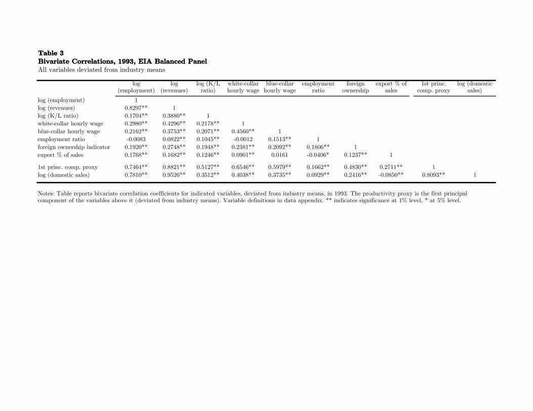
Table 3Table 3Table 3Table 3Bivariate Correlations, 1993, EIA Balanced PanelBivariate Correlations, 1993, EIA Balanced PanelBivariate Correlations, 1993, EIA Balanced PanelBivariate Correlations, 1993, EIA Balanced PanelAll variables deviated from industry means

log (employment) 1

log (revenues) 0.8297** 1

log (K/L ratio) 0.1704** 0.3880** 1

white-collar hourly wage 0.2980** 0.4296** 0.2178** 1

blue-collar hourly wage 0.2162** 0.3753** 0.2071** 0.4560** 1

employment ratio -0.0083 0.0822** 0.1045** -0.0012 0.1513** 1

foreign ownership indicator 0.1920** 0.2748** 0.1948** 0.2381** 0.2092** 0.1806** 1

export % of sales 0.1768** 0.1682** 0.1246** 0.0901** 0.0161 -0.0406* 0.1237** 1

1st princ. comp. proxy 0.7464** 0.8821** 0.5127** 0.6546** 0.5979** 0.1662** 0.4830** 0.2711** 1

log (domestic sales) 0.7810** 0.9526** 0.3512** 0.4038** 0.3735** 0.0929** 0.2416** -0.0850** 0.8093** 1

log (K/L ratio)

white-collar hourly wage

1st princ. comp. proxy

log (domestic sales)

Notes: Table reports bivariate correlation coefficients for indicated variables, deviated from industry means, in 1993. The productivity proxy is the first principal component of the variables above it (deviated from industry means). Variable definitions in data appendix. ** indicates significance at 1% level, * at 5% level.

blue-collar hourly wage

employment ratio

foreign ownership

export % of sales

log (employment)

log (revenues)

Table 4Table 4Table 4Table 4Differential Effects of Peso Crisis by Initial Productivity, EIA 1993-2001 Balanced PanelDifferential Effects of Peso Crisis by Initial Productivity, EIA 1993-2001 Balanced PanelDifferential Effects of Peso Crisis by Initial Productivity, EIA 1993-2001 Balanced PanelDifferential Effects of Peso Crisis by Initial Productivity, EIA 1993-2001 Balanced PanelProxy for productivity: first principal component of plant characteristics

Coeff. Estimate R-sqr. Coeff. Estimate R-sqr.

(1) (2) (3) (4)

Independent variables: productivity proxy (first principal component of initial-year characteristics), industry and state effects

Dependent variable:

∆ (export % of sales) 1.698*** 0.162 0.529** 0.136

[0.234] [0.223]

∆ log(white-collar wage) 0.067*** 0.151 0.002 0.092

[0.008] [0.007]

∆ log(blue-collar wage) 0.034*** 0.138 0.000 0.104

[0.006] [0.005]

∆ log(wage ratio) 0.036*** 0.087 0.001 0.085

[0.009] [0.008]

∆ log(K/L ratio) 0.067*** 0.114 0.035*** 0.11

[0.012] [0.012]

∆ log(employment ratio) -0.003 0.115 -0.005 0.112

[0.009] [0.008]

Period

1993-1997 1997-2001

Notes: All estimates by unweighted OLS. Coefficients estimates for productivity proxy in odd-numbered columns, R-squared for each regression in even-numbered columns. Productivity proxy calculated by taking first principal component of the following variables in the initial year, deviated from industry means: export % of sales, log(employment), log(K/L ratio), log(revenues), log(white-collar employment/blue-collar employment), log(white-collar wage), log(blue-collar wage), foreign ownership indicator. Level of a given variable is omitted from principal component calculation when its change is the dependent variable. In calculating the change in the wage ratio, the overall average wage is used to calculate principal component, rather than white-collar or blue-collar wage. Robust standard errors in brackets. N=3003 for all regressions. Further variable definitions in data appendix. *** indicates significance at 1% level, ** at 5% level, * at 10% level.

Table 5Table 5Table 5Table 5Differential Effects of Peso Crisis on Employment and Revenues by Initial Productivity, EIA 1993-2001 Balanced PanelDifferential Effects of Peso Crisis on Employment and Revenues by Initial Productivity, EIA 1993-2001 Balanced PanelDifferential Effects of Peso Crisis on Employment and Revenues by Initial Productivity, EIA 1993-2001 Balanced PanelDifferential Effects of Peso Crisis on Employment and Revenues by Initial Productivity, EIA 1993-2001 Balanced Panel

Coeff. Est. R-sqr. Coeff. Est. R-sqr. Coeff. Est. R-sqr. Coeff. Est. R-sqr.

(1) (2) (3) (4) (5) (6) (7) (8)

Independent variables: initial-year log(domestic sales), industry and state effects

Dependent variable:

∆ log(employment) 0.000 0.125 0.005 0.129 0.018*** 0.147 0.015*** 0.135

[0.007] [0.006] [0.006] [0.005]

∆ log(revenues) -0.004 0.176 0.014 0.175 0.008 0.206 0.014** 0.187

[0.010] [0.009] [0.007] [0.007]

Independent variables: productivity proxy (first principal component of initial-year characteristics), industry and state effects

∆ log(employment) 0.036*** 0.134 0.025*** 0.148

[0.008] [0.007]

∆ log(revenues) 0.055*** 0.186 0.029*** 0.209

[0.009] [0.008]

Notes: OLS estimates from unweighted regressions of variable in left-hand column on proxy (indicated above), industry and state effects. IV estimates from similar regressions treating initial years as 1994 and 1998 and instrumenting log domestic sales with previous year. First principal component extracted from the following variables in the initial year, deviated from industry means: export % of sales, log(employment), log(K/L ratio), log(revenues), log(white-collar employment/blue-collar employment), log(white-collar wage), log(blue-collar wage), foreign ownership indicator. Level of a given variable is omitted from principal component calculation when its change is the dependent variable. In calculating the change in the wage ratio, the overall average wage is used to calculate principal component, rather than white-collar or blue-collar wage. Robust standard errors in brackets. N=3003 for all regressions. Further variable definitions in data appendix. *** indicates significance at 1% level, ** at 5% level, * at 10% level.

Period

1993-1997 1997-2001

OLS IV OLS IV

Table 6Table 6Table 6Table 6Differential Effects of Peso Crisis by Initial Productivity, EIA 1984-2001 Balanced PanelDifferential Effects of Peso Crisis by Initial Productivity, EIA 1984-2001 Balanced PanelDifferential Effects of Peso Crisis by Initial Productivity, EIA 1984-2001 Balanced PanelDifferential Effects of Peso Crisis by Initial Productivity, EIA 1984-2001 Balanced PanelProxy for productivity: log domestic sales

Coeff. Est. R-sqr. Coeff. Est. R-sqr. Coeff. Est. R-sqr. Coeff. Est. R-sqr.

(1) (2) (3) (4) (5) (6) (7) (8)

Independent variables: initial-year log(domestic sales), industry and state effects

Dependent variable:

∆ (export % of sales) 0.743** 0.277 0.504* 0.269 1.170** 0.271 0.770** 0.257

[0.298] [0.285] [0.459] [0.377]

∆ log(white-collar wage) 0.036*** 0.25 0.000 0.234 0.062*** 0.311 -0.008 0.27

[0.012] [0.015] [0.016] [0.013]

∆ log(blue-collar wage) 0.01 0.298 0.004 0.288 0.029*** 0.31 0.005 0.242

[0.010] [0.012] [0.011] [0.012]

∆ log(wage ratio) 0.027* 0.263 -0.003 0.221 0.033** 0.269 -0.013 0.244

[0.014] [0.017] [0.017] [0.016]

∆ log(K/L ratio) 0.059* 0.274 0.071** 0.251 0.061** 0.26 0.006 0.24

[0.033] [0.036] [0.024] [0.028]

∆ log(employment ratio) 0.005 0.31 -0.02 0.275 0.049*** 0.316 0.009 0.27

[0.014] [0.015] [0.018] [0.013]

∆ log(employment) -0.003 0.343 -0.039*** 0.294 0.001 0.324 0.012 0.334

[0.009] [0.015] [0.013] [0.012]

∆ log(revenues) -0.037** 0.333 -0.091*** 0.403 0.001 0.311 -0.007 0.406

[0.015] [0.019] [0.022] [0.017]

Notes: All estimates by unweighted OLS. Coefficients estimates for log domestic sales in odd-numbered columns, R-squared for each regression in even-numbered columns. Data on exports vs. domestic sales not available prior to 1986, whence the choice of 1986-1989 as periodization in columns (1)-(2). Robust standard errors in brackets. N=706 for all regressions. Further variable definitions in data appendix. *** indicates significance at 1% level, ** at 5% level, * at 10% level.

Period1986-1989 1997-20011989-1993 1993-1997

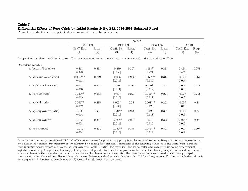
Table 7Table 7Table 7Table 7Differential Effects of Peso Crisis by Initial Productivity, EIA 1984-2001 Balanced PanelDifferential Effects of Peso Crisis by Initial Productivity, EIA 1984-2001 Balanced PanelDifferential Effects of Peso Crisis by Initial Productivity, EIA 1984-2001 Balanced PanelDifferential Effects of Peso Crisis by Initial Productivity, EIA 1984-2001 Balanced PanelProxy for productivity: first principal component of plant characteristics

Coeff. Est. R-sqr. Coeff. Est. R-sqr. Coeff. Est. R-sqr. Coeff. Est. R-sqr.

(1) (2) (3) (4) (5) (6) (7) (8)

Independent variables: productivity proxy (first principal component of initial-year characteristics), industry and state effects

Dependent variable:

∆ (export % of sales) 0.463 0.273 -0.279 0.267 1.183** 0.271 0.464 0.252

[0.328] [0.353] [0.471] [0.426]

∆ log(white-collar wage) 0.034*** 0.249 -0.005 0.235 0.066*** 0.314 -0.001 0.269

[0.013] [0.014] [0.016] [0.014]

∆ log(blue-collar wage) 0.011 0.298 0.001 0.288 0.029** 0.31 0.004 0.242

[0.010] [0.011] [0.012] [0.012]

∆ log(wage ratio) 0.029** 0.263 -0.007 0.221 0.045*** 0.274 -0.007 0.243

[0.013] [0.016] [0.017] [0.017]

∆ log(K/L ratio) 0.066** 0.275 0.065* 0.25 0.064*** 0.261 -0.007 0.24

[0.032] [0.035] [0.023] [0.030]

∆ log(employment ratio) -0.002 0.31 -0.034** 0.279 0.025 0.307 -0.006 0.27

[0.014] [0.015] [0.018] [0.015]

∆ log(employment) 0.015* 0.347 -0.029** 0.287 0.01 0.325 0.026** 0.34

[0.008] [0.014] [0.012] [0.012]

∆ log(revenues) -0.014 0.324 -0.039** 0.375 0.051*** 0.321 0.017 0.407

[0.014] [0.019] [0.018] [0.018]

Notes: All estimates by unweighted OLS. Coefficients estimates for productivity proxy in odd-numbered columns, R-squared for each regression in even-numbered columns. Productivity proxy calculated by taking first principal component of the following variables in the initial year, deviated from industry means: export % of sales, log(employment), log(K/L ratio), log(revenues), log(white-collar employment/blue-collar employment), log(white-collar wage), log(blue-collar wage), foreign ownership indicator. Level of a given variable is omitted from principal component calculation when its change is the dependent variable. In calculating the change in the wage ratio, the overall average wage is used to calculate principal component, rather than white-collar or blue-collar wage. Robust standard errors in brackets. N=706 for all regressions. Further variable definitions in data appendix. *** indicates significance at 1% level, ** at 5% level, * at 10% level.

Period1986-1989 1997-20011989-1993 1993-1997

Table 8Table 8Table 8Table 8Differential Effects of Peso Crisis by Initial Productivity, Selection-Correction Model, EIA 1993-2001 Unbalanced PanelDifferential Effects of Peso Crisis by Initial Productivity, Selection-Correction Model, EIA 1993-2001 Unbalanced PanelDifferential Effects of Peso Crisis by Initial Productivity, Selection-Correction Model, EIA 1993-2001 Unbalanced PanelDifferential Effects of Peso Crisis by Initial Productivity, Selection-Correction Model, EIA 1993-2001 Unbalanced PanelProxy for productivity: log domestic sales

Coeff. Est. chi-sqr. Coeff. Est. chi-sqr.

(1) (2) (3) (4)

Independent variables: initial-year log(domestic sales), industry and state effects

Dependent variable:

First stage: Remains in sample 0.239*** 241.2 0.354*** 334.2

[0.032] [0.032]

Second stage: ∆ (export % of sales) 1.917*** 874.8 0.473* 767.2

[0.305] [0.250]

∆ log(white-collar wage) 0.059*** 694.1 0.012 607.8

[0.011] [0.009]

∆ log(blue-collar wage) 0.027*** 699.7 -0.003 644.3

[0.008] [0.007]

∆ log(wage ratio) 0.032*** 500.1 0.016 577.6

[0.012] [0.010]

∆ log(K/L ratio) 0.063*** 622.1 -0.002 655.5

[0.017] [0.015]

∆ log(employment ratio) 0.015 577.8 0.013 666.1

[0.012] [0.010]

∆ log(employment) 0.004 684.2 0.013* 786.6

[0.009] [0.008]

∆ log(revenues) 0.011 848.8 0.014 1067.0

[0.013] [0.010]

N (remain in sample) 3297 3003

N (exit) 308 294

N (total) 3605 3297

Notes: Estimates follow the two-step selection-correction procedure of Heckman (1976), with a first-stage probit and second-stage OLS with an inverse Mills ratio term. Estimates are unweighted. Coefficients estimates for log(domestic sales) in odd-numbered columns, chi-squared statistic for test that all coefficients (except the intercept) are zero in even-numbered columns. Standard errors in brackets. Monetary values in 1994 pesos. *** indicates significance at 1% level, ** at 5% level, * at 10% level.

Period1993-1997 1997-2001

Table 9Table 9Table 9Table 9Summary Statistics by Maquiladora and Export Status, ENESTyC, 1992, 1995, 1999Summary Statistics by Maquiladora and Export Status, ENESTyC, 1992, 1995, 1999Summary Statistics by Maquiladora and Export Status, ENESTyC, 1992, 1995, 1999Summary Statistics by Maquiladora and Export Status, ENESTyC, 1992, 1995, 1999

Maquilas Non-exp Exporters All Maquilas Non-exp Exporters All Maquilas Non-exp Exporters All

ISO 9000 certification Mean 0.2 0.0 0.1 0.0 0.5 0.1 0.3 0.2

S.D. 0.4 0.2 0.3 0.2 0.5 0.2 0.4 0.4

White-collar avg. schooling Mean 12.0 11.7 12.6 12.0 12.6 11.3 12.9 12.1

S.D. 1.8 2.6 1.6 2.3 2.4 3.0 2.0 2.7

Blue-collar avg. schooling Mean 6.7 6.9 7.4 7.0 7.2 7.6 8.2 7.7

S.D. 1.2 1.6 1.5 1.6 1.4 1.9 1.6 1.7

Absentee rate Mean 3.1 3.6 2.7 3.2 1.1 1.4 1.2 1.3 1.3 1.2 1.0 1.1

S.D. 2.4 2.9 2.5 2.7 0.9 1.0 1.0 1.0 1.1 1.0 0.9 1.0

Accident rate Mean 4.5 2.8 3.4 2.9 2.2 2.1 2.8 2.3

S.D. 3.4 4.5 4.1 4.4 2.6 3.3 3.2 3.2

Formal training indicator Mean 0.65 0.29 0.66 0.39 0.49 0.26 0.68 0.34 0.82 0.32 0.73 0.52

S.D. 0.5 0.5 0.5 0.5 0.5 0.4 0.5 0.5 0.4 0.5 0.4 0.5

Turnover rate Mean 130.2 72.9 82.4 78.3 121.4 48.7 60.0 51.5 111.4 52.6 73.3 68.0

S.D. 112.6 117.0 92.9 113.4 64.8 66.5 56.7 65.5 67.0 63.7 59.6 66.7

% manual equipment Mean 26.8 25.2 21.5 24.5 26.4 38.7 23.3 32.3

S.D. 33.9 35.3 29.7 34.2 30.3 38.1 30.4 35.6

Employment Mean 439.7 137.4 415.1 214.8 261.6 81.4 278.4 117.7 505.2 116.4 364.8 252.1

S.D. 237.4 207.9 249.4 253.0 218.1 141.9 202.2 172.8 224.4 191.7 256.3 267.9

White-collar % of emp. Mean 18.7 32.0 31.8 31.0 15.9 34.7 31.5 34.0 17.7 36.5 28.3 31.0

S.D. 10.6 28.8 17.7 26.3 12.6 32.8 20.5 30.9 15.9 31.5 19.9 27.4

White-collar hourly wage Mean 3.02 2.98 4.07 3.32 4.62 2.82 4.21 3.30 3.89 2.53 4.03 3.35

S.D. 1.3 1.7 1.8 1.8 2.6 2.0 2.2 2.2 2.5 1.9 2.5 2.4

Blue-collar hourly wage Mean 1.03 0.99 1.28 1.05 1.09 1.04 1.32 1.10 1.15 0.91 1.16 1.03

S.D. 0.4 0.4 0.4 0.4 0.5 0.5 0.5 0.5 0.4 0.4 0.5 0.5

N 394 3049 1213 4656 78 3591 1560 5229 589 4115 2168 6872

Notes: Table reports means and standard deviations (not standard errors) weighted by ENESTyC sampling weights times employment. Variable definitions in data appendix.

1999

Non-maquilas

1992

Non-maquilas

1995

Non-maquilas

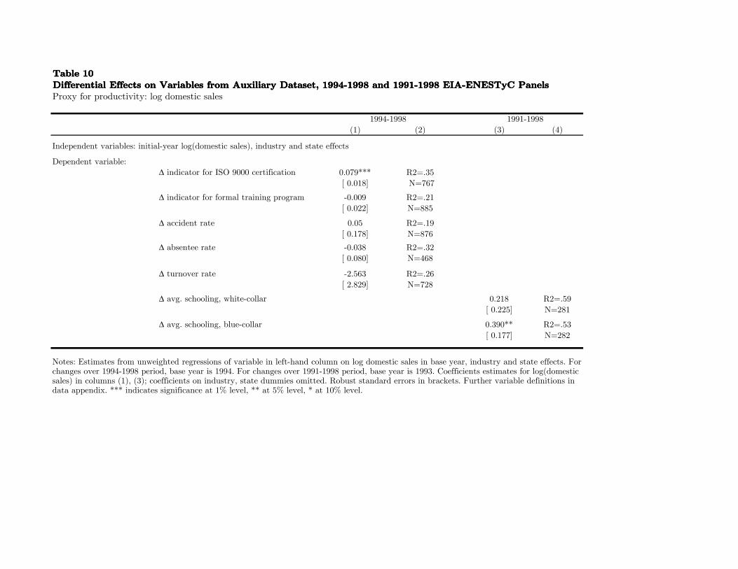
Table 10Table 10Table 10Table 10Differential Effects on Variables from Auxiliary Dataset, 1994-1998 and 1991-1998 EIA-ENESTyC PanelsDifferential Effects on Variables from Auxiliary Dataset, 1994-1998 and 1991-1998 EIA-ENESTyC PanelsDifferential Effects on Variables from Auxiliary Dataset, 1994-1998 and 1991-1998 EIA-ENESTyC PanelsDifferential Effects on Variables from Auxiliary Dataset, 1994-1998 and 1991-1998 EIA-ENESTyC PanelsProxy for productivity: log domestic sales

(1) (2) (3) (4)

Independent variables: initial-year log(domestic sales), industry and state effects

Dependent variable:

∆ indicator for ISO 9000 certification 0.079*** R2=.35

[ 0.018] N=767

∆ indicator for formal training program -0.009 R2=.21

[ 0.022] N=885

∆ accident rate 0.05 R2=.19

[ 0.178] N=876

∆ absentee rate -0.038 R2=.32

[ 0.080] N=468

∆ turnover rate -2.563 R2=.26

[ 2.829] N=728

∆ avg. schooling, white-collar 0.218 R2=.59

[ 0.225] N=281

∆ avg. schooling, blue-collar 0.390** R2=.53

[ 0.177] N=282

1994-1998 1991-1998

Notes: Estimates from unweighted regressions of variable in left-hand column on log domestic sales in base year, industry and state effects. For changes over 1994-1998 period, base year is 1994. For changes over 1991-1998 period, base year is 1993. Coefficients estimates for log(domestic sales) in columns (1), (3); coefficients on industry, state dummies omitted. Robust standard errors in brackets. Further variable definitions in data appendix. *** indicates significance at 1% level, ** at 5% level, * at 10% level.

Notes: Each point represents one 4-digit industry (rama ); see data appendix for description of industry categories. Data on employment in 1988 and 1998 and capital in 1998 from the Censos Industriales (Industrial Censuses). Data on schooling is from Encuesta Nacional de Empleo Urbano (ENEU), a household survey similar to the CPS for full-time employees (male and female), ages 12-64, in 16 cities in original ENEU sample.

Fig. 1b: Shift Toward Less Capital-Intensive IndustriesFig. 1b: Shift Toward Less Capital-Intensive IndustriesFig. 1b: Shift Toward Less Capital-Intensive IndustriesFig. 1b: Shift Toward Less Capital-Intensive Industries

-0.5

0

0.5

1

1.5

2 3 4 5 6 7

log capital-labor ratio, 1998

∆ lo

g em

plo

ym

ent,

198

8-19

98

Fig. 1a: Shift Toward Less Skill-Intensive IndustriesFig. 1a: Shift Toward Less Skill-Intensive IndustriesFig. 1a: Shift Toward Less Skill-Intensive IndustriesFig. 1a: Shift Toward Less Skill-Intensive Industries

-0.5

0

0.5

1

1.5

6 7 8 9 10 11 12

average schooling, 1998

∆ lo

g em

plo

ym

ent,

198

8-19

98

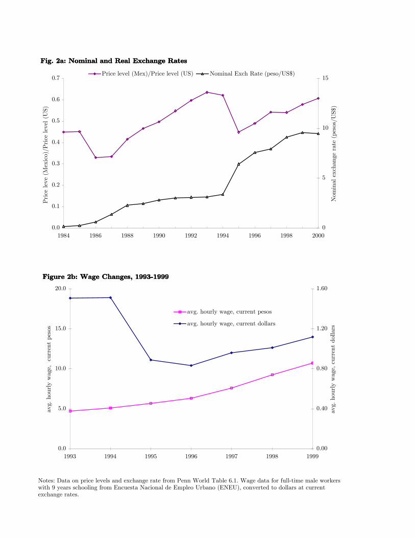
Notes: Data on price levels and exchange rate from Penn World Table 6.1. Wage data for full-time male workers with 9 years schooling from Encuesta Nacional de Empleo Urbano (ENEU), converted to dollars at current exchange rates.

Fig. 2a: Nominal and Real Exchange RatesFig. 2a: Nominal and Real Exchange RatesFig. 2a: Nominal and Real Exchange RatesFig. 2a: Nominal and Real Exchange Rates

0.0

0.1

0.2

0.3

0.4

0.5

0.6

0.7

1984 1986 1988 1990 1992 1994 1996 1998 2000

Pri

ce lev

e (M

exic

o)/P

rice

lev

el (

US)

0

5

10

15

Nom

inal

exch

ange

rat

e (p

esos

/US$)

Price level (Mex)/Price level (US) Nominal Exch Rate (peso/US$)

Figure 2b: Wage Changes, 1993-1999Figure 2b: Wage Changes, 1993-1999Figure 2b: Wage Changes, 1993-1999Figure 2b: Wage Changes, 1993-1999

0.0

5.0

10.0

15.0

20.0

1993 1994 1995 1996 1997 1998 1999

avg.

hou

rly w

age,

cu

rren

t pes

os

0.00

0.40

0.80

1.20

1.60

avg.

hou

rly w

age,

curr

ent

dol

lars

avg. hourly wage, current pesos

avg. hourly wage, current dollars

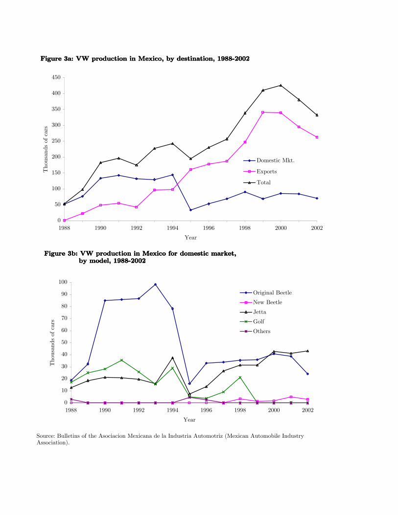
Source: Bulletins of the Asociacion Mexicana de la Industria Automotriz (Mexican Automobile Industry Association).

0

50

100

150

200

250

300

350

400

450

1988 1990 1992 1994 1996 1998 2000 2002

Year

Thou

sands

of c

ars

Domestic Mkt.

Exports

Total

Figure 3a: VW production in Mexico, by destination, 1988-2002Figure 3a: VW production in Mexico, by destination, 1988-2002Figure 3a: VW production in Mexico, by destination, 1988-2002Figure 3a: VW production in Mexico, by destination, 1988-2002

Figure 3b: VW production in Mexico for domestic market,Figure 3b: VW production in Mexico for domestic market,Figure 3b: VW production in Mexico for domestic market,Figure 3b: VW production in Mexico for domestic market, by model, 1988-2002 by model, 1988-2002 by model, 1988-2002 by model, 1988-2002

0

10

20

30

40

50

60

70

80

90

100

1988 1990 1992 1994 1996 1998 2000 2002

Year

Thou

sands

of c

ars

Original Beetle

New Beetle

Jetta

Golf

Others

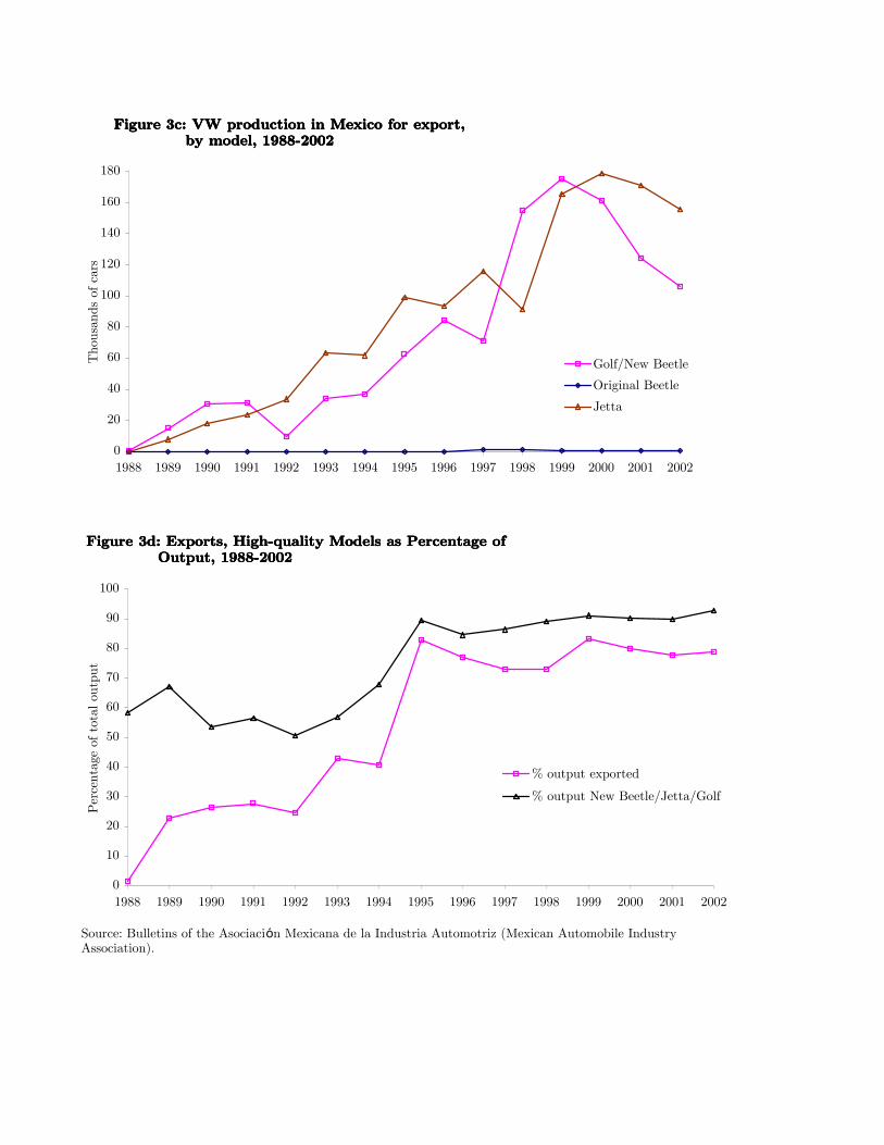
Source: Bulletins of the Asociación Mexicana de la Industria Automotriz (Mexican Automobile Industry Association).

Figure 3d: Exports, High-quality Models as Percentage ofFigure 3d: Exports, High-quality Models as Percentage ofFigure 3d: Exports, High-quality Models as Percentage ofFigure 3d: Exports, High-quality Models as Percentage of Output, 1988-2002 Output, 1988-2002 Output, 1988-2002 Output, 1988-2002

0

10

20

30

40

50

60

70

80

90

100

1988 1989 1990 1991 1992 1993 1994 1995 1996 1997 1998 1999 2000 2001 2002

Per

centa

ge o

f to

tal ou

tput

% output exported

% output New Beetle/Jetta/Golf

Figure 3c: VW production in Mexico for export, Figure 3c: VW production in Mexico for export, Figure 3c: VW production in Mexico for export, Figure 3c: VW production in Mexico for export, by model, 1988-2002 by model, 1988-2002 by model, 1988-2002 by model, 1988-2002

0

20

40

60

80

100

120

140

160

180

1988 1989 1990 1991 1992 1993 1994 1995 1996 1997 1998 1999 2000 2001 2002

Thou

sands

of c

ars

Golf/New Beetle

Original Beetle

Jetta

Notes: Data from EIA 1993-2001 Balanced Panel. Export percentage of total sales calculated as total exports for all plants/total sales for all plants. Plants with exports greater than zero classified as exporting.

0

50

100

150

200

250

300

350

1993 1994 1995 1996 1997 1998 1999 2000 2001

millions

1994 p

esos

export sales domestic sales total sales

Fig. 4a: Sales, Domestic and Export, 1993-2001Fig. 4a: Sales, Domestic and Export, 1993-2001Fig. 4a: Sales, Domestic and Export, 1993-2001Fig. 4a: Sales, Domestic and Export, 1993-2001 Fig. 4b: Export percentage of total salesFig. 4b: Export percentage of total salesFig. 4b: Export percentage of total salesFig. 4b: Export percentage of total sales

0

5

10

15

20

25

30

35

1993 1994 1995 1996 1997 1998 1999 2000 2001

Fig. 4c: Percentage of Plants ExportingFig. 4c: Percentage of Plants ExportingFig. 4c: Percentage of Plants ExportingFig. 4c: Percentage of Plants Exporting

20

30

40

50

1993 1994 1995 1996 1997 1998 1999 2000 2001

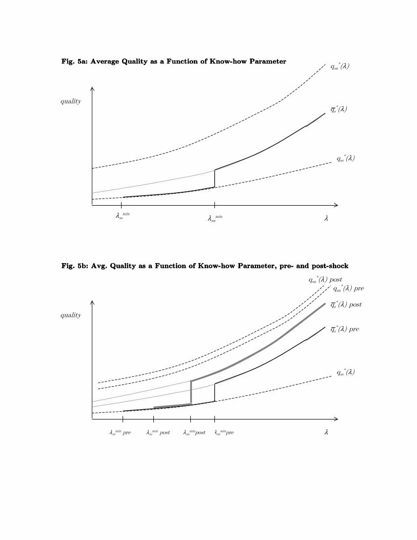
Fig. 5a: Average Quality as a Function of KnowFig. 5a: Average Quality as a Function of KnowFig. 5a: Average Quality as a Function of KnowFig. 5a: Average Quality as a Function of Know----how Parameterhow Parameterhow Parameterhow Parameter

Fig. 5b: Avg. Quality as a Function of KnowFig. 5b: Avg. Quality as a Function of KnowFig. 5b: Avg. Quality as a Function of KnowFig. 5b: Avg. Quality as a Function of Know----how Parameter, prehow Parameter, prehow Parameter, prehow Parameter, pre---- and post and post and post and post----shockshockshockshock

λ

quality

λsnmin

qsn*(λ)

qss*(λ)

qs*(λ)

λ

quality

λsnminpre

qss*(λ)

qs*(λ) pre

qsn*(λ) post

λssmin pre λss

min post

qs*(λ) post

λsnminpost

λssmin

qsn*(λ) pre

Fig. 5c: Change iFig. 5c: Change iFig. 5c: Change iFig. 5c: Change in Average Quality as a Function of Known Average Quality as a Function of Known Average Quality as a Function of Known Average Quality as a Function of Know----how Parameterhow Parameterhow Parameterhow Parameter

λ

quality

λsnminpre

dqs*(λ)

λssmin pre λss

min post λsnminpost

Fig. 6: Differential Effect of Peso Crisis by Degree of Engagement in Export MarketFig. 6: Differential Effect of Peso Crisis by Degree of Engagement in Export MarketFig. 6: Differential Effect of Peso Crisis by Degree of Engagement in Export MarketFig. 6: Differential Effect of Peso Crisis by Degree of Engagement in Export Market

Fig. 6a: Revenues

9.4

9.8

10.2

10.6

11

1993 1994 1995 1996 1997 1998 1999 2000 2001

log r

eal re

ven

ues

always non-exporters

switchers into exporting

always exporters

Fig. 6b: Employment

4.5

4.75

5

5.25

5.5

5.75

1993 1994 1995 1996 1997 1998 1999 2000 2001

log e

mplo

ym

ent

always non-exporters

switchers into exporting

always exporters

Fig. 6c: White-collar Wage

2.3

2.5

2.7

2.9

3.1

3.3

1993 1994 1995 1996 1997 1998 1999 2000 2001

log r

eal w

hit

e co

llar

wage

always non-exporters

switchers into exporting

always exporters

Fig. 6d: Blue-collar Wage

1.3

1.5

1.7

1.9

2.1

2.3

1993 1994 1995 1996 1997 1998 1999 2000 2001

log r

eal blu

e-co

llar

wage

always non-exporters

switchers into exporting

always exporters

Fig. 7: Non-Parametric Regressions, Levels of Key Variables vs. log Domestic Sales, 1993 and 1997Fig. 7: Non-Parametric Regressions, Levels of Key Variables vs. log Domestic Sales, 1993 and 1997Fig. 7: Non-Parametric Regressions, Levels of Key Variables vs. log Domestic Sales, 1993 and 1997Fig. 7: Non-Parametric Regressions, Levels of Key Variables vs. log Domestic Sales, 1993 and 1997

Notes: All variables deviated from industry means. Graphs are locally smoothed non-parametric regressions (bandwidth = .5), of levels of indicated variables in indicated year on log domestic sales in 1993, using EIA 1993-2001 Balanced Panel.

Fig. 7a: Export % of Sales

-3

-2

-1

0

1

2

3

4

-3 -2 -1 0 1 2 3log domestic sales 1993

export

% o

f sa

les

1994

1997

Fig. 7b: White-collar wage

-0.75

-0.5

-0.25

0

0.25

0.5

0.75

-3 -2 -1 0 1 2 3log domestic sales 1993

log r

eal w

hit

e-co

llar

wage

1993

1997

Fig. 7c: Blue-collar wage

-0.75

-0.5

-0.25

0

0.25

0.5

0.75

-3 -2 -1 0 1 2 3

log domestic sales 1993

log r

eal blu

e-co

llar

wage

1993

1997

Fig. 7d: Wage ratio

-0.3

-0.2

-0.1

0

0.1

0.2

0.3

-3 -2 -1 0 1 2 3

log domestic sales 1993

log w

age

ratio

1993

1997

Fig. 8: Non-Parametric Regressions, Changes 1993-1997 and 1997-2001Fig. 8: Non-Parametric Regressions, Changes 1993-1997 and 1997-2001Fig. 8: Non-Parametric Regressions, Changes 1993-1997 and 1997-2001Fig. 8: Non-Parametric Regressions, Changes 1993-1997 and 1997-2001

Notes: All variables deviated from industry means. Graphs are locally smoothed non-parametric regressions (bandwidth = .5), of changes of indicated variables over indicated periods on log domestic sales in initial year (1993 or 1997), using EIA 1993-2001 Balanced Panel. For export percentage, changes omit initial year to avoid bias from mean reversion.

Fig. 8a: Changes in export percentage of sales

-4

-3

-2

-1

0

1

2

3

-3 -2 -1 0 1 2 3

log domestic sales, initial year

∆ ex

port

% o

f sa

les

change 1994-1997

change 1998-2001

Fig. 8b: Changes in white-collar wage

-0.2

-0.1

0

0.1

0.2

-3 -2 -1 0 1 2 3

log domestic sales, initial year

∆ lo

g r

eal w

hit

e-co

llar

wage

change 1993-1997

change 1997-2001

Fig. 8c: Changes in blue-collar wage

-0.2

-0.1

0

0.1

0.2

-3 -2 -1 0 1 2 3

log domestic sales, initial year

∆ lo

g r

eal blu

e-co

llar

wage

change 1993-1997

change 1997-2001

Fig. 8d: Changes in wage ratio

-0.1

-0.05

0

0.05

-3 -2 -1 0 1 2 3

log domestic sales, initial year

∆ lo

g w

age

ratio

change 1993-1997

change 1997-2001