NBER WORKING PAPER SERIES

TRADE REFORMS AND MARKET SELECTION:EVIDENCE FROM MANUFACTURING PLANTS IN COLOMBIA

Marcela EslavaJohn C. HaltiwangerAdriana D. Kugler

Maurice Kugler

Working Paper 14935http://www.nber.org/papers/w14935

NATIONAL BUREAU OF ECONOMIC RESEARCH1050 Massachusetts Avenue

Cambridge, MA 02138April 2009

We thank Diana Hincapie, Rafael Santos, and Camilo Morales for excellent research assistance, andRoberto Alvarez, Mary Amiti, Orazio Attanasio, Sebastian Edwards, Ricardo Hausmann, Larry Kleinman,Ralf Martin, Alejandro Micco, Nina Pavcnik, Carmen Pages, Dani Rodrik, Chad Syverson and Johnvan Reenen as well as participants at numerous seminars and conferences. Support was provided byNSF Grant SES-0617816, the Tinker Foundation, the IDB, and a GEAR grant from the Universityof Houston. We are also grateful to the National Planning Department for providing data on tariffs,and to DANE for access to the Manufacturing Survey and advice about its use. The views expressedherein are those of the author(s) and do not necessarily reflect the views of the National Bureau ofEconomic Research.

© 2009 by Marcela Eslava, John C. Haltiwanger, Adriana D. Kugler, and Maurice Kugler. All rightsreserved. Short sections of text, not to exceed two paragraphs, may be quoted without explicit permissionprovided that full credit, including © notice, is given to the source.

Trade Reforms and Market Selection: Evidence from Manufacturing Plants in ColombiaMarcela Eslava, John C. Haltiwanger, Adriana D. Kugler, and Maurice KuglerNBER Working Paper No. 14935April 2009JEL No. F43,L25,O47

ABSTRACT

We use plant output and input prices to decompose the profit margin into four parts: productivity,demand shocks, mark-ups and input costs. We find that each of these market fundamentals are importantin explaining plant exit. We then use variation across sectors in tariff changes after the Colombiantrade reform to assess whether the impact of market fundamentals on plant exit changed with increasedinternational competition. We find that greater international competition magnifies the impact of productivity,and other market fundamentals, on plant exit. A dynamic simulation that compares the distributionof productivity with and without the trade reform shows that improvements in market selection fromtrade reform help to weed out the least productive plants and increase average productivity. In addition,we find that trade liberalization increases productivity of incumbent plants and improves the allocationof activity within industries.

Marcela EslavaUniversidad de Los AndesCarrera 1 Este No 18 A -70. Bloque CBogota, Colombiameslava@uniandes.edu.co

John C. HaltiwangerDepartment of EconomicsUniversity of MarylandCollege Park, MD 20742and NBERhaltiwan@econ.umd.edu

Adriana D. KuglerUniversity of HoustonDepartment of Economics204 McElhinney HallHouston, TX 77204-5019and NBERadkugler@uh.edu

Maurice KuglerHarvard UniversityCenter for International Development79 JFK StreetCambridge, MA 02138andWilfrid Laurier Universitymaurice_kugler@harvard.edu

1 Introduction

It is clear that an important means by which market economies restructure and innovate

is through the entry and exit of establishments. Consistent with that view, in economies

like the U.S., the entry and exit process has been identi�ed as an important component

of aggregate productivity growth. Aggregate productivity growth is achieved, in part, by

the ongoing market selection process that involves the exit of low productivity businesses

and the entry of businesses that exhibit either higher relative productivity at entry or

rapid productivity growth in their �rst few years.1

Given the importance of business turnover for productivity growth, rigid market

institutions and concentrated market structures can be expected to a¤ect aggregate

productivity by raising barriers to both entry and exit. Barriers on either margin are

likely to reduce the overall pace of �rm and establishment turnover and to generate

misallocation of activity in the economy. Recent theoretical models, indeed, show that

poor market institutions (including trade barriers) generate misallocation by introduc-

ing idiosyncratic distortions to pro�tability (see Banerjee and Du�o (2005), Hsieh and

Klenow (2009), Restuccia and Rogerson (2008), and Bartelsman et al. (2008)).

Surprisingly, early evidence for developing economies shows that the pace of estab-

lishment turnover is typically not that di¤erent from that observed for industrialized

economies.2 This is at odds with the idea that developing economies, which are typi-

cally subject to more restrictive institutions, should have a slower pace of reallocation.

On the other hand, recent �ndings from both emerging and transition economies suggest

that market reforms improve allocative e¢ ciency (e.g., Bartelsman et al. (2008), Eslava

et al. (2004, 2006, 2009)). By contrast to these recent studies, in this paper, we explore

the link between market selection and a particular area of market reform �namely, trade

liberalization.

Trade liberalization has been a core component of market reforms in developing

economies and, in particular, in Latin America. Trade liberalization could a¤ect plant

exits and productivity through a number of channels. First, as Pavcnik (2002) and

others argue, increased international competition may induce incumbent �rms to become

more productive.3 Second, Melitz (2003) shows that trade liberalization could force

1See, e.g., Baily, Campbell and Hulten (1992), Bartelsman and Doms (2000), Foster, Haltiwanger

and Krizan (2001), Foster, Haltiwanger and Syverson (2008), and Olley and Pakes (1996).2See, e.g., Bartelsman et al. (2008) and Tybout (2000).3A number of studies �nd that productivity of incumbent producers increases after trade opening,

including: Levinsohn (1993) for Turkey, Harrison (1994) for Cote d�Ivoire, Tybout and Westbrook

2

lower productivity �rms out of the market, cutting o¤ the lower tail of the productivity

distribution. In a related vein, Restuccia and Rogerson (2008) show that less regulated

environments enhance the role of productivity as a determinant of plant survival. In

our empirical analysis we focus on the direct and indirect impacts of trade on exits, as

suggested by the recent literature.

An important aspect of trade opening in Colombia is that it varied widely across

sectors. This between-sector, within country, variation re�ects substantial di¤erences in

tari¤ changes across di¤erent sectors, as well as substantial di¤erences in initial tari¤

levels. The large variation in the extent of trade opening across sectors, along with rich

longitudinal establishment-level data for the manufacturing sector of Colombia provides

a unique opportunity to explore the impact of trade liberalization on market selection.

Not only do we explore the direct impact of the reduction of trade barriers on exits, but

we also explore how reduced trade barriers a¤ected the role of market fundamentals on

plant exits in Colombia. In particular, we explore how trade liberalization a¤ected the

role of idiosyncratic (i.e., plant-level) total factor productivity, demand shocks, mark-

ups and cost variation. Finally, we explore whether increased exit of low productivity

plants following trade reform leads to increases in average productivity.4

A novel feature of our analysis is the separate measurement of physical productivity

(rather than revenue-based productivity), idiosyncratic demand, mark-ups and input

costs, which allows us to evaluate separately the impact that each of these determinants

has on plant exit. By contrast, previous analyses of exit patterns after trade liberalization

rely on reduced form plant characteristics related to survival, such as size and age, rather

than market fundamentals which directly determine exit (e.g., Gibson and Harris (1996),

Baggs (2005), and Bernard and Jensen (2007)). Unlike previous analyses, we are able to

measure these fundamentals separately because the Colombian Manufacturing Survey

allows to construct plant-level prices of both inputs and outputs. This unique feature of

(1995) for Mexico, Pavcnik (2002) for Chile, Tre�er (2004) for Canada, Topalova (2004) for India, and

Fernandes (2007) for Colombia.4In our earlier work (i.e., Eslava et al. (2006)), we show that some market fundamentals became

more important determinants of plant exit in the 1990s relative to the 1980s in Colombia. The 1990s

was a period of market reforms on many dimensions including trade, �nancial market, labor market,

privatization, and tax reforms. In contrast to this paper, our earlier work made no attempt to identify

the impact of particular reforms on market selection, and did not exploit the cross-sectional variation of

regulations. Moreover, our earlier work also had less detailed measures of fundamentals (e.g., we lacked

a measure of market power). Finally, our earlier work did not look at the implications of selection for

average productivity, nor did it explore some of the alternative channels of the impact of trade reform

on aggregate productivity that we study here.

3

the data is useful for our purposes in several ways. First, we are able to de�ate output

with plant-speci�c de�ators, leading to a measure of TFP that has been stripped of

idiosyncratic demand e¤ects. Our approach contrasts with most of the literature, where

the measurement of TFP uses plant-level revenue de�ated with a sector-level price index.

Given within sector price variability, the standard estimation of TFP confounds high

physical e¢ ciency and high prices. Second, we are able to estimate demand shocks at

the plant level due to the availability of plant-level output prices. In our estimation

of the demand process, we also allow mark-ups to vary across plants. Consistent with

theories of market selection, we �nd that plants with higher productivity, those facing

lower input prices, and those subject to positive demand shocks and with more inelastic

demands, are less likely to exit.

Moreover, we �nd that market fundamentals (with the exception of the mark-up)

become more important in determining plant survival, as competition increases due to

trade opening. In particular, we �nd that the marginal e¤ect of productivity on exit

increases in sectors facing declines in tari¤s. Given improved market selection, we explore

the implications for aggregate productivity by conducting a dynamic counterfactual

simulation of the exit process under two scenarios: one with the actual tari¤ levels and

another one leaving the tari¤s at their initial, 1984, levels. We �nd an increase in average

plant-level productivity of about 3.3 log points due to improved market selection with

the actual tari¤s relative to the 1984 tari¤s. This analysis is novel, as previous studies

do not explore the impact of increased selectivity in plant exits on average productivity

after trade opening.5

In addition, we consider some alternative channels through which trade liberalization

can a¤ect productivity to put our �ndings on market selection in context. In particular,

following Pavcnik (2002), we use a di¤erences-in-di¤erences speci�cation to quantify

the impact of trade reform on within plant productivity growth for continuing plants.

Our results reinforce Pavcnik�s (2002) main �nding that trade opening increases within-

plant productivity growth, making use of the improved measures of trade opening and

productivity that are available for Colombia. In particular, we use tari¤s that vary

within-sector and over time, while in the Chilean case studied by Pavcnik tari¤s varied

only over time so that tari¤ reductions had to be captured through time dummies in

her analysis. In addition, our TFP measure captures physical productivity rather than

a revenue-based measure of productivity which combines withing sector di¤erences in

5See, e.g., Gibson and Harris (1996) for New Zeland�s trade liberalization; Head and Ries (1999)

and Baggs (2005) for Canada and NAFTA; Bernard and Jensen(2007) for FDI in the United States.

4

prices and physical e¢ ciency e¤ects. Another channel we explore is whether trade

opening strengthens the relationship between market size and productivity as discussed

by Olley and Pakes (1996) and Bartelsman et al. (2008). We �nd, indeed, that sectors

facing lower tari¤s show larger correlations between market share and productivity,

indicating that trade opening increases the share of productive plants and reduces the

market share of less productive plants.

The rest of the paper proceeds as follows. In Section 2, we discuss the theoretical

considerations that motivate our empirical analysis. In Section 3, we describe the market

reforms introduced in Colombia during the 1990s. In Section 4, we present the data from

the Annual Manufacturing Survey. In Section 5, we show our results on the impact of

the pro�t margin components, and the interaction of these market fundamentals with

trade reforms on exit probabilities. In Section 6, we present the implications of trade-

related exits for average productivity and explore alternative channels through which

tari¤ reductions may have a¤ected productivity. We conclude in Section 7.

2 Theoretical Considerations

According to selection models of industry dynamics (e.g., Jovanovic (1982), Hopenhayn

(1992), Ericson and Pakes (1995)) producers should continue operations if the discounted

value of future pro�ts exceeds the opportunity cost of remaining in operation. At the

same time, recent models (e.g., Melitz (2003), Melitz and Ottaviano (2008), and Foster et

al. (2008)) emphasize that many market fundamentals in�uence variation in pro�tabil-

ity across producers. In this literature, producers with market power make decisions on

outputs, inputs, and output prices, given productivity shocks, demand shocks, demand

elasticity and input price shocks drawn by the producer from a joint distribution. These

models also assume that �rms face frictions in the market through entry barriers. Typ-

ically, producers are assumed not to know their market fundamentals prior to entry,

pay an entry fee and obtain their �rst draw of their market fundamentals from a joint

distribution. The market fundamentals are assumed to evolve stochastically over time

and consistent with the recent empirical literature are assumed to be highly persistent

processes. Given �xed costs of operating each period, the producer makes a decision on

whether or not to stay or exit at each point in time. As derived in the recent literature,

the canonical exit decision can be modeled as being given by:6

6See, e.g., Melitz and Ottaviano (2008) and Foster et al. (2008) for models that yield exit speci�ca-

tions with this full list of market fundamentals (or plant pro�t-margin components).

5

ejt =

(1 if PDV f�(TFPjt; PIjt; Djt; "jt)� Cjtg < 00 if PDV f�(TFPjt; PIjt; Djt; "jt)� Cjtg � 0

That is, plant j exits if the expected present net discounted value of pro�ts including

the �xed cost of operating Cjt is negative.7 Current and future expected pro�ts, �,

(and, in turn, their present discounted value, PDV) gross of �xed costs are a positive

function of demand, Djt and productivity shocks, TFPjt, a positive function of the

demand elasticity, "jt (where the latter is negative so an increase implies an increase in

the mark-up) and a decreasing function of input price shocks, PIjt.

In what follows, we estimate this speci�cation of market selection for Colombia. The

estimates for the basic model are of interest in their own right, since Colombia is unique

in having rich data with plant-level measures of each of these fundamentals, including

demand shocks and demand elasticities. Our primary purpose is, however, to explore

the role of market reforms and, in particular, trade liberalization on the market selection

process.

Theory suggests that trade liberalization enhances the mechanism that drives low

productivity and other under-performing plants out of the market. For example, Melitz

(2003) develops a monopolistic competition model where trade liberalization impacts

market selection through equilibrium wages. As the economy liberalizes, the more pro-

ductive plants expand by increasing exports and this drives up the equilibrium wage.

With a higher wage, only incumbents with productivity above a larger threshold survive.

At the same time, Bernard et al. (2003) introduce stochastic plant productivity in a

perfect competition Ricardian model where producers from the same country compete

to be the sole national supplier to speci�c destinations. Lower trade barriers bump

out low-productivity plants due to import competition, while high productivity plants

grow into export markets. As labor shifts from low-productivity exiting plants to high-

productivity expanding plants, there is a rise in aggregate productivity.8

7The �xed cost of operating Cjt should be de�ned as being net of the option value for the plant of

waiting to exit. This option value arises due to the irreversibility stemming from sunk entry costs.8Our empirical analysis is closer to Bernard et al. (2003), as we focus on the e¤ects of trade reform on

market selection for a given set of fundamentals. By contrast, Melitz (2003) and Melitz and Ottaviano

(2008) emphasize how exit will be impacted by trade through changes in fundamentals (i.e., wages and

mark-ups, respectively). While these channels are likely important, studying the impact of trade on

wages empirically requires richer wage data than we have from the Monthly Manufacturing Survey.

For instance, the studies by Goldberg and Pavcnik (2005) and Attanasio et al. (2004) highlight the

complex mechanisms through which trade may a¤ect average wages and the distribution of wages using

6

Another channel suggested by the recent literature on misallocation and productiv-

ity (e.g., Banerjee and Du�o (2005), Hsieh and Klenow (2009), Restuccia and Rogerson

(2008) and Bartelsman et al. (2008)) is the increased relative importance of market

fundamentals for exit when trade is liberalized. In these models, distortions to markets

include an idiosyncratic component. In our context, trade barriers potentially yield idio-

syncratic distortions as they may vary across sectors yielding more favorable treatment

for some �rms and less favorable treatment of other �rms. A key insight from this class

of models is that, in addition to the pro�t-margin components discussed above, these

idiosyncratic distortions impact pro�tability and, in turn, market selection. Thus, in

the presence of idiosyncratic distortions, a plant�s survival becomes less related to its

favorable pro�t-margin fundamentals, and more to regulations. For instance, protec-

tions (including trade protections) to speci�c sectors may allow �rms in these sectors to

survive even with relatively low productivity. On the other hand, when these protections

are eliminated, �rms will only be able to survive if they have relatively high productivity.

Given the possible mechanisms through which trade liberalization can impact market

selection, our empirical strategy is based on an enhanced model of exit which includes

idiosyncratic market distortions:

ejt =

(1 if PDV f�(TFPjt; PIjt; Djt; "jt; � jt)� Cjtg < 00 if PDV f�(TFPjt; PIjt; Djt; "jt; � jt)� Cjtg � 0

where � jt represents market distortions for plant j including those from trade barriers.

While we are not able to measure the full set of market distortions impacting any

given plant, we have one good measure of distortions, namely tari¤s. A key working

hypothesis of our empirical analysis is that the plants in sectors with the largest decreases

in tari¤s are, holding other things equal (e.g., including other reforms), more likely to

have seen a larger reduction in their market distortions. As noted above, a key insight

from the recent literature is that the presence of idiosyncratic distortions across plants

reduces the marginal e¤ect of fundamentals on the probability of exit.9 This insight helps

guide and interpret our empirical speci�cation of the market selection models presented

below. Our core identifying assumption is that sectors with greater tari¤ reductions

household data for Colombia. Exploring the impact of trade liberalization via changes in mark-ups

would require a careful and detailed study of mark-ups similar to the studies of trade on wages by

Goldberg and Pacvnik (2005) and Attanasio et al. (2004). Exploring these alternative channels is an

interesting area we intend to study in future work.9The analysis in Bartelsman et al. (2008) shows that an increase in the dispersion of idiosyncratic

distortions decreases the marginal e¤ect of market fundamentals, like productivity, on plant exit.

7

have had a larger reduction in market distortions and, accordingly, fundamentals should

become incrementally more relevant for market selection in the sectors with greater tari¤

declines. As will become clear, in practice when we estimate the above speci�cation, we

include controls and estimate �exible speci�cations, including both direct and interaction

e¤ects, to capture the impact of trade and other reforms.

3 Trade Reforms in Colombia

Colombia underwent substantial changes in trade policy during the past three decades.

After considerable trade liberalization in the 1970s, the administration of president Belis-

ario Betancurt implemented a reversal towards protection during the early 1980s in re-

sponse to the appreciation of the exchange rate, which had contributed to increased

foreign competition. Betancurt�s policies increased the average tari¤ level to 27 percent

in 1984, but the degree of protection across industries was far from uniform. Manu-

facturing sectors bene�ted the most from increased protection as the average tari¤ in

manufacturing rose to 50 percent. However, even within manufacturing some sectors

received more protection than others. The sector with the highest protection was tex-

tiles and apparel, which had nominal tari¤s of nearly 90 percent, and wood products

followed with a nominal tari¤ of 60 percent. These two sectors also had the highest

levels of protection through non-tari¤ barriers.

While barriers to trade were reduced in the second half of the 1980s, trade was

largely liberalized in Colombia during the �rst half of the 1990s. Figure 1 shows average

e¤ective tari¤s and the standard deviation of e¤ective tari¤s starting in 1984.10 From

this initial level, the �gure shows a substantial decline both in average e¤ective tari¤s

and the dispersion of these tari¤s in 1985. The �gure then shows a gradual decrease

in tari¤s which started during the administration of president Virgilio Barco in the late

1980s.

In 1990, the administration of president Cesar Gaviria introduced a comprehensive

reform package, which included measures to modernize the state and liberalize markets.

Reforms during the 1990s occurred in the areas of trade, �nancial and labor markets,

privatization and the tax system.11 Probably the most important of all these reforms10The e¤ective tari¤ for a given �nal good adjusts the nominal tari¤ levied to the good itself, by

substracting the weighted sum of tari¤s on the inputs used to produce that good, where the weights

are given by the share of the input in production costs for that good (using the corresponding entry in

the Input-Output table).11A number of studies have examined the impacts of non-trade reforms on workers and �rms. Kugler

8

was the trade reform carried out at the beginning of the 1990s.

The average nominal tari¤ declined from 27 to about 10 percent overall, and from 50

to 13 percent in manufacturing, between 1984 and 1998. As Figure 1 shows, there was a

drastic drop in average e¤ective tari¤s and in the dispersion of e¤ective tari¤s between

1990 and 1992 during the Gaviria administration. By 1992, the average e¤ective tari¤

was at 26.6% compared to 62.5% in 1989 and compared to 86% in 1984. Similarly, the

dispersion of tari¤s fell substantially during the early 1990s, though dispersion across

industries still remained substantial as the standard deviation of tari¤s remained at

around 0.2.

After Gaviria�s term, Ernesto Samper won the presidential election in 1994 based

on a platform which partly opposed trade liberalization and other reforms.12 While the

new government did not dismantle the existing reforms at the time, it managed to stop

the momentum for further liberalization. This is clear in Figure 1, which shows that the

average and standard deviation of e¤ective tari¤s remain �at after 1992.

The description above makes clear that there were important changes in both the

mean level and the dispersion of tari¤s across sectors. An interesting aspect of the

Colombian trade reforms is that at the same time that the overall level of protection

was lowered, the sectoral structure of protection was also substantially altered as barriers

to trade were lowered to similar levels across sectors irrespective of their initial level.

The identi�cation strategy of our analysis of the e¤ect of market reforms on market

selection exploits this cross-sectional variation in tari¤ reductions.

4 Data

Since we are interested in estimating the impact of market fundamentals on exit as

trade opens, we require information on tari¤s, and on plant characteristics, including:

productivity, demand shocks, demand elasticities, and input prices. Also, to control

for other ongoing reforms that may had coincided with the trade reforms, in some

speci�cations we require a measure of other regulations. In this section, we provide a

(1999, 2005) studies the impact of the 1991 labor market reforms, Kugler and Kugler (2009) studies

the impact of the 1993 payroll tax reform; Kugler (2006) studies the impact of the 1992 FDI reform,

and Eslava et al. (2009) study the impact of the 1991 labor and capital market reforms.12Note that the Colombian electoral system at the time ruled out re-election after one term in o¢ ce,

which may help explain the depth of the structural reforms in Colombia in the absence of an economic

crisis.

9

description of the data, and we then explain the measurement of physical productivity

and demand shocks.

4.1 Data Description

We use data from the Colombian Annual Manufacturing Survey (AMS), an unbalanced

panel that registers information on all manufacturing establishments with 10 or more

employees. Establishments with less than 10 employees but with a nominal value of

production over a certain level are also included.13 Given that these requirements are

satis�ed, a plant is then included in our sample in a given year if it reports positive

production for that year. We have data covering the 1982-1998 period, at an annual

frequency. The AMS records include information on the value of production, number

of employees, value of materials used, physical units of energy demanded, value of the

stock of capital and purchases of capital, as well as the quantities of each product it

manufactures and of each material it uses.

4.1.1 Plant-level Prices of Inputs and Output

We start by constructing output and material price indices for each establishment, using

the information on individual products and materials for each plant. To create a plant-

level index of material prices, we �rst calculate weighted averages of the price changes

of all individual materials used by the plant.14 The weight assigned to each input

corresponds to the average share (over the whole period) of that input in the total value

of materials used by the plant.15 Plant-level price indices are then generated recursively

from these plant-level price changes, where we set 1982 as the base year. Given the

recursive method used to construct the price indices and the fact that we do not have

plant-level information for material prices for the years before plants enter the sample,

13For instance, for 1998 the value limit was set at U$35,000.14Since some large outliers appear, we trim the 1% percent tails of the distribution of plant-level

price changes. In addition, given that the in�ation rate in Colombia has hovered around 18% during

the period, we choose to drop observations that show reductions of prices beyond 50% in absolute value

or increases in prices beyond 200%.15An alternative speci�cation would be to use a Divisia index approach letting the share in any given

year be the average of the share in the current and prior year. We have used this alternative approach

and obtain similar results. However, we �nd some anomalous large and transitory �uctuations in the

shares suggesting problems with measurement error. Given these concerns, we use a more conservative

approach using the average over the entire period.

10

we replace missing values with the average material price in the plant�s sector, location,

and year.16 A similar method is used to construct output price indices.

We use plant-level output prices to construct physical quantities of output, which are

measured as the nominal output de�ated by the plant-level price index. Similarly, we

construct physical quantities of materials used as the nominal value of these materials

de�ated by the plant-level materials price index. Physical quantities of energy usage are

directly reported at the plant-level.

4.1.2 Capital Stock

We construct a series of the capital stock for each plant, j, following the perpetual

inventory method. Gross investment is generated from the information on �xed assets

reported by each plant, using the expression:

Ijt = KNFjt �KNI

jt � djt � �Ajt,

where KNFjt is the reported �nal value of �xed assets by plant j at the end of year t;

KNIjt is the reported initial value of �xed assets reported by plant j at the start of year

t, djt is the depreciation reported by plant j at the end of year t, and �Ajt is the reported

in�ation adjustment to �xed asset value by plant j at the end of year t (only relevant

since 1995, the �rst year in which plants were required by law to consider this component

in their calculations of end-of-year �xed assets). We de�ate gross investment using a

de�ator for capital formation from National Accounts�Input-Output matrices (or the

equivalent �output utilization matrices�since 1994); the de�ator varies in general at the

2-digit sector level, and for a few sectors at a higher level of disaggregation. Denote this

de�ator as DS(j)t where S(j) is the sector to which plant j belongs. The plant capital

stock is, thus, constructed recursively following:

Kjt =�1� �S(j)

�Kjt�1 +

IjtDS(j)t

,

where �S(j) is the depreciation rate for the 3-digit sector to which plant j belongs calcu-

lated by Pombo (1999). We initialize the capital stock for each plant using the nominal

capital stock �rst ever recorded (at the beginning of year), KNIjt0, de�ated by the average

capital de�ator for the current and previous years, DS(j)t0 and DS(j)t0�1:

16When the information is not available by location, we impute the national average in the sector

for that year. This imputation assumes that the plant that is about to enter would have had a similar

product mix as existing plants in the same sector-location-year.

11

Kjt0 =KNIjt0

12(DS(j)t0 +DS(j)t0�1)

:

4.1.3 Employment

The level of employment or the number of workers is reported directly by each estab-

lishment. Since hours per worker are not reported in the AMS, we construct a measure

of labor usage, by using information on average wages at the 3-digit sector level from

the Monthly Manufacturing Survey.17 Our measure of hours per worker in sector S(j)

to which plant j belongs is:

HS(j)t =earningsS(j)t

wS(j)t;

where wS(j)t is the measure of sectoral hourly wages at the 3-digit level, and earningsS(j)tis a measure of earnings per worker constructed from our data as

earningsS(j)t =

Pj2S

payrolljtPj2S

Ljt.

4.1.4 Descriptive Statistics of Plant-level variables

Table 1 presents descriptive statistics of the quantity and price variables just described.18

The price and quantity variables are expressed in logs. We restrict our sample to plants

in three-digit sectors with more than 25 establishments in the average year, since we

make use of within-sector variation in our analysis below. In the next section, we use

the variables summarized in Table 1 to estimate the production function and inverse-

demand equation.

Table 1 also shows entry and exit rates. A plant is classi�ed as entering in t if it

exists in our sample in year t but not in t� 1. Similarly, the plant exits in t if it exists17Data on sector wages are reported separately for production and non-production workers. We use

a weighted average of the wages of those two categories, where the weights are the shares of each type

of worker in total sector employment. We de�ate the nominal wages using the CPI obtained from the

National Department of Statistics.18The descriptive statistics capture both within industry as well as between industry variation. In the

empirical analysis, we always control for industry e¤ects, so we focus our attention on within industry

variation (across plants and across time) in our estimation. Interestingly, we have generated a version

of Table 1 that removes industry e¤ects and �nd very similar patterns, suggesting that much of the

between plant variation in outputs, inputs and prices re�ects within industry variation.

12

in the sample in t but not in t + 1. Note that Table 1 reports entry and exit rates of

7% and 9% respectively, somewhat lower than those reported for developed countries

(Davis et al. (1996)). These lower entry and exit rates for Colombia are consistent with

the perception that developing economies are subject to greater rigidities than more

developed countries (see Tybout (2000) for a discussion of this issue).

4.1.5 Tari¤s and Reform data

Our data on e¤ective tari¤s come from the National Planning Department. E¤ective

tari¤s are available at the product level for each year, using a classi�cation system (and

therefore product identi�ers) that were created for the Andean Community. Since the

tari¤s�database also assigns each of these products a four-digit sector ISIC code, we

can construct e¤ective tari¤s at the four-digit level by averaging e¤ective tari¤s across

products in a given sector. The only other study of the impact of trade liberalization

on productivity with a similar level of disaggregation of tari¤s is that by Tre�er (2004).

Having e¤ective tari¤s at this high level of dissagregation allows us to still control for

sector e¤ects in our estimation, using 2-digit sector dummies which may capture other

factors a¤ecting exits. On the other hand, the fact that we use sector-level rather than

plant-level tari¤s reduces concerns about tari¤s being in�uenced by individual �rms. In

addition, we limit our analysis to 3-digit sectors with more than 25 establishments in the

average year. Moreover, as a robustness check, we drop the most concentrated sectors

(based on a Her�ndahl Index) from our analysis and �nd no di¤erences with our results

based on the overall sample.

We also use an index of reforms other than trade in some of our speci�cations.

We construct this index from the institutions index produced by Lora (2001). Lora

generates indices of market reform in each of �ve areas: labor regulation, �nancial

sector regulation, trade openness, privatization and taxation. He then averaged those

individual indices to construct an index of overall reform. The indices for individual

areas of regulation fall in a 0-1 scale, where 0 (1) corresponds to the most (least) rigid

institutions in Latin America over the period for each of the �ve categories that compose

the aggregate index. We modify Lora�s index in two ways. First, we exclude trade reform

from the calculation of the overall index, since we look at trade institutions directly

through tari¤s. Second, we use a di¤erent 0-1 scale, where the index in each category

is calculated relative to the minimum and maximum level of reform in Colombia during

the period, rather than relative to the minimum and maximum for Latin America. The

Lora index is only available since 1985, so that the regression analysis that includes this

13

index as a control is restricted to the period 1985-1998.

The evolution of the means and standard deviations of e¤ective tari¤s, as well as

the index of other reforms (which only varies over time) are shown in Figure 1. As

described above, both the mean and the standard deviation of e¤ective tari¤s go down

signi�cantly between 1984 and 1992, and then show little variation. Figure 1 also shows

that the index of other reforms, which goes up during the 1990s when market reforms are

implemented, increased at the same time that tari¤s were being reduced. This highlights

the importance of controlling for other reforms in our estimation.

4.2 Estimation of Productivity and Demand Shocks

We begin by estimating production and demand functions at the plant level, to obtain

measures of TFP, demand shifters and the elasticity of demand. Following Eslava et

al. (2004), our TFP estimates are constructed using factor elasticities estimated using

downstream demand to instrument inputs, while our demand estimation uses TFP as

an instrument.

4.2.1 Total Factor Productivity

We estimate total factor productivity for plant j in year t as the residual from a pro-

duction function:

Yjt = K�jt(LjtHjt)

�E jtM�jtVjt;

where, Yjt is output, Kjt is capital, Ljt is total employment, Hjt are hours per worker,

Ejt is energy consumption, Mjt are materials, and Vjt is a productivity shock.

Our total factor productivity measure is estimated as:

TFPjt = log Yjt � b� logKjt � b�(logLjt + logHjt)� b logEjt � b� logMjt: (1)

where b�, b�, b , and b� are the estimated factor elasticities for capital, labor hours, energy,and materials. Since productivity shocks are likely to be correlated with inputs, OLS

estimates of factor elasticities are likely to be biased. We thus rely on IV estimates, where

the instruments are demand shifters, input prices, and government spending which are

likely correlated with input but uncorrelated with productivity shocks. A more detailed

description of this estimation and its results can be found in Eslava et al. (2004).19

19Although the sample di¤ers slightly because we drop observations from sectors with few establish-

ments, the estimated factor elasticities we report here are the same as those in Eslava et al. (2004) up

to the second decimal place.

14

Table 2 presents summary statistics for our TFP measure estimated with instrumen-

tal variables (labeled TFP in this Table), and compares it to alternative measures of

productivity. All statistics are computed at the three-digit level. We compare our IV

TFP measure with a TFP measure estimated using cost shares at the 3-digit level as

factor elasticities (TFPC) and with a TFP measure estimated using factor elasticities

from an OLS estimation of the production function (TFPO). Our TFP measure is highly

correlated with both of these alternatives, with correlation coe¢ cients above 0.85. Thus,

in spite of the di¤erences in estimated factor elasticities obtained using various methods,

we �nd that the TFP distribution across plants is similar.20 The similarity between our

TFP measure and the cost shares TFP measure suggests that allowing factor elasticities

to vary across sectors is not crucial for TFP estimation in our data. In the rest of the

paper, we rely on TFP estimates based on our IV estimation.

Table 2 also shows other interesting patterns that we exploit in our analysis in the

following sections. First, the table shows considerable dispersion in plant-level prices

and TFP within sectors, which is consistent with the association between price and

productivity dispersion and frictions pointed out in recent literature. In addition, price

dispersion is consistent with the common assumption of product di¤erentiation in the

recent literature.

Second, Table 2 shows that TFP (measured either using our preferred measure in row

1 of Table 2 or TFPC which uses the cost share factor elasticities) is inversely correlated

with plant-level prices. This is consistent with more productive plants or industries

having lower marginal costs and setting lower prices when faced with downward sloping

demand curves.21 We exploit this inverse relationship to estimate demand elasticities

20The �nding that the distribution of plant-level TFP is robust to alternative estimation methods

is analogous to related �ndings by van Biesebroeck (2006). There are alternative ways to estimate

factor elasticities in the literature such as Olley and Pakes (1996) and Blundell and Bond (1999). The

Olley and Pakes method (and related methods in the literature) uses a proxy approach to deal with

endogenous factors of production. However, as discussed in Foster et al. (2008), these proxy methods

are less suitable for speci�cations with both demand shocks and productivity shocks (there is an omitted

variable problem in the proxy inversion). Nonetheless, we generated TFP measures using proxy methods

and also �nd that the resulting TFP measures are highly correlated with our TFP measure estimated

using instrumental variables.21One possible concern in interpreting this inverse correlation between TFP and prices is division

bias. TFP is physical output per unit input but physical output is based on the ratio of nominal output

to plant-level prices. If there is measurement error in prices this can yield an inverse correlation in TFP

and prices. To explore the relevance of this concern, we also have estimated the correlation between

lagged TFP and current prices. If measurement error in plant-level prices is white noise then this

15

and demand shocks in the next section. This �nding is also useful to provide insights

as to the underlying sources and interpretations of price variation. As noted, price

dispersion is consistent with product di¤erentiation. This product di¤erentiation may

re�ect horizontal or vertical di¤erentiation. As such, some of the price variation may

re�ect product quality variation. While it is obviously of interest to ultimately sort out

the nature of this product di¤erentiation, this is not the focus of the current analysis.

However, we note that the inverse correlation between TFP and prices is consistent

with more e¢ cient producers moving along downward sloping demand curves.22 For our

purposes, then, if plant-level prices in part re�ect variation in product quality (as well

as potentially other sources of idiosyncratic demand shocks), our underlying assumption

is that such variation in product quality is not correlated with TFP so that TFP serves

as a good instrument for the output price in the demand function.23

Table 2 also illustrates the importance of being able to measure plant-level prices

and physical e¢ ciency. TFP2 is a measure of �revenue�productivity, similar to that

used more frequently in the literature, given the absence of plant-level prices. Similar

to the other measures of productivity we have reported, it is calculated using equation

(1), but where Yjt is plant-level output divided by sectoral-level price indices and Mjt

is expenditures on materials divided by sectoral-level materials price indices. Although

TFP and TFP2 are positively related, the correlation coe¢ cient is only 0.68, signi�cantly

below the correlation of TFP with both TFPC and TFPO, where the latter all use plant

level prices. Moreover, TFP2 is essentially uncorrelated with plant-level prices. Indeed,

the relation between prices and productivity, which we exploit in our data to identify

demand elasticities and shocks, disappears when sector-level de�ators are used. The

reason for this is straightforward: variation in TFP2 directly re�ects the variation in

prices, and the resulting positive correlation with plant-level prices o¤sets the negative

correlation between prices and physical productivity (TFP).

4.2.2 Demand Estimation

While productivity is likely to be one of the crucial components of pro�tability, as

discussed in Section 2, other components are also probably important determinants of

eliminates the division bias. The average within sector correlation of lagged TFP and current prices is

-0.59 which is similar in magnitude to the -0.65 correlation between TFP and prices in Table 2.22We �nd that this inverse correlation holds for all 3-digit sectors.23If productivity shocks and product quality were positively related, we would be more likely to

observe a positive correlation between TFP and prices.

16

pro�tability and survival. For example, even if plants are highly productive, they may

be forced to exit the market if faced with large negative idiosyncratic demand shocks.

Another important determinant of exits is likely to be the degree of market power of

a producer, which empirically can be captured by the mark-up or the inverse of the

demand elasticity. In this section, we describe how we estimate both the demand shocks

as well as demand elasticities.

Our demand shock measure is estimated as the residual from estimating a demand

equation, which in its simplest form may be written (in logs) as:

log Yjt = "j logPjt + logDjt:

In this case, the demand shock is estimated using the following expression:

djt = log cDjt = log Yjt + b"j logPjt; (2)

where djt is the demand shock faced by �rm j at time t and b"j is the estimated elasticityof demand, which may potentially vary across plants or sectors and which is strictly

negative in the presence of a downward sloping demand.

Using OLS to estimate the demand function is likely to generate an upwardly biased

estimate of demand elasticities because demand shocks are positively correlated to both

output and prices, so that b" will be smaller in absolute value than the true ": To eliminatethe upward bias in our estimates of demand elasticities, we use TFP as an instrument

for Pjt since TFP is negatively correlated with prices but unlikely to be correlated

with demand shocks (Eslava et al. (2004)).24 Also, to avoid potential problems from

measurement error and associated division bias, we use lagged TFP as the instrument.

Columns (1) and (2) of Table 3 report the OLS and IV results from the simple demand

equation. For consistency with other estimations reported below, the estimation is done

pooling establishments from all sectors and controlling for sector e¤ects at the 2-digit

24In the macro literature on TFP there is considerable attention paid to measured cyclical �uctuations

in TFP being associated with unmeasured changes in factor utilization (see, e.g., Basu and Fernald

(2000)). As such, at the aggregate level, the assumption of measured TFP and aggregate demand

shocks being uncorrelated may be problematic. However, we are mostly exploiting cross sectional

variation in plant-level TFP with the variance of idiosyncratic shocks an order of magnitude larger

than any aggregate shocks. Moreover, the idiosyncratic TFP and demand shocks we estimate are

highly persistent suggesting that issues about cyclical factor utilization are dwarfed by the highly

persistent idiosyncratic shocks (thus, inducing relatively little idiosyncratic variation in unmeasured

factor utilization). Also, to the extent that energy usage proxies for capacity utilization, we would be

taking the utilization factor out of our TFP measure.

17

level. We control for sector e¤ects to control for unobserved sectoral heterogeneity and

we estimate robust standard errors.25 OLS results presented in Column (1) yield an

estimated elasticity of -0.87. Meanwhile, IV results in Column (2), which use (lagged)

TFP as an instrument, show a much higher average elasticity (in absolute value) of -2.12.

We also estimate a di¤erent demand speci�cation, in which we let the demand elas-

ticity vary over time and by a plant�s location. To do this, we include the density of

roads in the state in which the plant is located both as a control and as an interaction

variable in the demand speci�cation. The idea behind including density of roads is that

this is a good proxy for access to markets, so that we should expect demand to increase

as the density of roads increases and also competition to increase as access to markets

improves. In this case, the demand equation may be written as,

log Yjt = �0+�1 logPjt+�2DensityR(j)t+�3DensityR(j)t�logPjt+ S(j)+�R(j)+logDjt;

whereDensityR(j)t is measured in kilometers of paved roads per square kilometer of total

area of the state R(j) in which plant j is located, S(j) are 2-digit sector e¤ects and

�R(j) are region (state) e¤ects.26 The latter control for unobserved sectoral and regional

heterogeneity. In particular, region �xed e¤ects are added to control for unobserved

factors at the region level that may drive demand as well as be correlated with road

density. As in the previous case, we estimate robust standard errors. We also include

national level GDP growth as an additional control, to make sure that the variation of

roads over time is not simply re�ecting other aggregate e¤ects. In this case, the demand

shock is again estimated as the components of demand after abstracting from the impact

of price, while the demand elasticity may be written as:

b"R(j)t = �1 + �3DensityR(j)t: (3)

Column (3) of Table 3 reports results for this speci�cation. As expected, we �nd that

increased road density increases the demand for output. Also, increased road density25Wooldridge (2002) notes that in models with unobserved heterogeneity at the group level assump-

tions need to be made about the form of this heterogeneity. One could assume that the unobserved

heterogeneity is not correlated with the RHS variables and then use random e¤ect estimators and/or

clustered standard error corrections as appropriate. He notes that permitting �xed e¤ects that are

potentially correlated with RHS variables is more robust than these alternatives but also notes that

robust standard error estimators are required. It is this latter approach that we use throughout this

analysis.26The density measure varies across states and over di¤erent decades (1980s and 1990s). The data

were provided by CEDE.

18

increases the demand elasticity (in absolute terms), consistent with the idea that greater

competition due to greater access to markets makes demand more responsive to changes

in prices.27

In what follows, we use the estimates of demand shocks and elasticities from Table

3 in our analysis of the impact of market fundamentals on plant exit. As will become

clear, we explore analyses using the estimates from both Columns (2) and (3) of Table

3.

5 E¤ects of Market Fundamentals and Tari¤s on

Plant Exit

5.1 The Role of Market Fundamentals for Selection

As discussed in Section 2, the characterization of the exit decision implies that the plant

ceases operations if its net present discounted value of pro�ts (inclusive of �xed costs

of operating) is negative. Assuming that the �xed cost, ujt, is drawn from a normal

distribution, we can in practice estimate a plant�s probability of exit using a probit

model, where we specify the probability of exit between t and t + 1 as a function of

measures of market fundamentals in period t� 1:28

Pr(ejS(j)R(j)t) = Pr(�S + �GGDPt + �1TFPjt�1 + P0

Ijt�1�2 + �3Djt�1 + �4"R(j)t�1 � ujt);

(4)

where ejs(j)R(j)t takes the value of 1 if the plant j in sector S(j) and region R(j) exits

between periods t and t + 1; �S are 2-digit industry e¤ects; GDPt is the growth of

27It would be interesting to explore demand structures that permit richer variation in plant-level

mark-ups. Another idea suggested to us by Chad Syverson would be to use our data to compute plant-

speci�c mark-ups directly. That is, use our plant-speci�c cost data to estimate marginal costs and then

compute mark-ups at the plant-level. Investigating the properties of such mark-ups including how they

vary across di¤erent types of plants and how they may have changed in response to market reforms is

an interesting empirical agenda that we plan to pursue in future related work.28To justify a probit we require that there be some unobserved heterogeneity beyond the fundamentals

that we measure to account for the variation in the data on plant exit. One obvious candidate is

variation in the �xed cost of operating each period. Alternatively, there could be some other component

of operating pro�ts that is unobserved but uncorrelated with the fundamentals that we do observe. For

ease of exposition, we refer to this stochastic unobserved heterogeneity as a stochastic �xed cost in the

text.

19

aggregate gross domestic product in year t; TFPjt�1 measures productivity in period

t� 1, PIjt�1 is a vector of energy and materials prices in period t� 1; Djt�1 is a demand

shifter in period t�1; "R(j)t�1 is the price elasticity of demand for plant j in region R(j)in period t� 1, and ujt is an i.i.d. normally distributed error term. In what follows, weconsider alternative speci�cations of this basic equation using the alternative measures

of market fundamentals that we have developed in the analysis above.29

Table 4 reports summary statistics for the determinants of exit included in equation

(4) (except for input prices which are reported in Table 1), as well as for e¤ective tari¤s

and indices of other reforms, which will be included in an expanded speci�cation. The

sample has been limited to the observations that enter those estimations. Since the

index of other reforms is only available since 1985, our estimation period for the exit

equations is 1985-1998.

Table 5 reports the marginal e¤ects obtained from estimating the baseline speci�-

cation in equation (4), as well as speci�cations with additional more controls in each

subsequent column. In all the speci�cations in Table 5, we include 2-digit sector �xed

e¤ects to control for unobserved sectoral heterogeneity and we estimate robust standard

errors. Marginal e¤ects are calculated setting all right-hand-side variables at their mean

levels. Column (1) reports the e¤ect of productivity and input prices on plant exit when

2-digit sector �xed e¤ects and aggregate GDP growth are included, but idiosyncratic

demand e¤ects are left out. As expected, higher lagged productivity is negatively related

to the probability of exit, while higher lagged energy and material prices are positively

related with the probability of leaving the market. In particular, a one standard devi-

ation increase in TFP from its mean level yields a 1.1 percentage point decrease in the

probability of exit, and one standard deviation increase in energy and material prices

yield respective increases of 0.35 and 0.6 percentage points in the probability of exit.30

Since the average exit probability is 9%, these e¤ects, especially the one associated with

29We use fundamentals dated at time t� 1 to predict exit from t to t+ 1 given possible incomplete

measurement and endogeneity issues in period t (the period just prior to exit). Our data are calendar

year data but there may be mid-year exits which may yield measurement error in fundamentals for part

year plants. Moreover, if the process of exit itself as the plant shuts down impacts fundamentals there

is a problem of reverse causality. The use of period t� 1 information mitigates both of these concerns.30Note that because our exit model is not linear and because one standard deviation changes in the

fundamentals are not marginal changes, these e¤ects cannot be simply obtained by multiplying the

change in the fundamental by its marginal e¤ect. We obtain them by evaluating the probability of exit

when one fundamental is one standard deviation away from its mean and the others are at their means,

and calculating the di¤erence between that probability and the probability of exit when all regressors

are at their means.

20

TFP, re�ect large percentage changes in the probability of exit.

Columns (2) to (4) of Table 5 report results including idiosyncratic demand e¤ects.

Column (2) includes the output price as a rough control for demand, while Columns (3)

and (4) include our measures of demand shifts and elasticities. The results in Column

(3) use the demand shocks from Column (2) of Table 3 �this is the relevant speci�cation

when we do not permit elasticities to vary across plants. For this speci�cation, we �nd

that a one standard deviation increase in TFP and demand yields respective reductions of

1.2 and 3.1 percentage points in the probability of exit, while a one standard deviation

increase in energy and material prices yield a 0.4 and 0.8 percentage points increase,

respectively, in the probability of exit.31

When we permit elastiticies to vary across plants consistent with Column (3) of Table

3 (where elasticities vary with road density), a one standard deviation demand shock

yields a 3 percentage points reduction in the probability of exit. A one standard deviation

increase in the price elasticity reduces the probability of exit by 0.28 percentage points.

Since the price elasticity of demand is strictly negative, a larger demand elasticity (i.e.,

closer to zero) is associated with more inelastic demand, so that more market power

reduces exit. The e¤ects of TFP and input prices are very similar in Columns (3) and

(4).

To help put the results in this section into perspective, we note that many empirical

papers on market selection include controls for plant size and age and �nd that younger

and smaller plants are more likely to exit. In our view, these variables are typically

included to proxy for unobserved market fundamentals. In our case, we have a very

rich set of fundamentals that are motivated by the theory. For example, our demand

shock measure captures variation in scale not driven by variation in productivity, and

thus we do not include size as a control. Put di¤erently, our scale measure emerges

directly from the theory while typical measures of size (e.g., total number of employees)

are endogenous and functions of the market fundamentals that we have measured. We

note, however, that a case could be made for inclusion of an endogenous state variable

related to size �namely the capital stock. As a robustness check, we estimated similar

speci�cations to those in Table 5 but also including the lagged capital stock and found

that these results are robust to inclusion of this variable. Moreover, we found that

31We report results with the output price included directly into the exit equation in Column (2)

to show that the e¤ect of the demand shock is similar whether we disaggregate the mark-up and

idiosyncratic demand or whether we take a rougher measure. To the extent that there are any concerns

about being able to separate the demand shock and elasticities, it is reassuring to note that the results

in Column (2) and those in Columns (3) and (4) are similar.

21

plants with a bigger capital stock are associated with a lower probability of exit. We do

not include capital either in the baseline speci�cation when we examine the interaction

with tari¤s, to keep the focus on market fundamentals. However, in unreported results

available upon request, we �nd that subsequent analysis to also be robust to the inclusion

of capital.32

Finally, we note that while we have a very rich set of fundamentals that capture a

great deal of variation across plants, it is possible that some unobserved heterogeneity

in the fundamentals underlying current and future expected pro�tability remains. This

might mean, for example, that estimated e¤ects of the observed cost variables are also

capturing the e¤ects of unobserved cost factors that are correlated with the observed

measures. For many of the purposes of this paper, this is not a critical concern since we

would still interpret our results as providing insights into the role of market fundamentals

for market selection. However, as exploratory analysis and as a robustness check we

estimated the speci�cations in Table 5 as linear probability models with establishment

�xed e¤ects.33 Interestingly, we �nd that our results are robust to this speci�cation.

In fact, we �nd that the marginal e¤ects of TFP, energy prices, demand and market

power become larger when plant e¤ects are included. We found this robustness check

reassuring but regard our baseline speci�cation as being more closely tied to the theory

where plants receive draws from the distribution of market fundamentals with plant-level

persistence in these draws.

5.2 The Interaction of Tari¤s and Market Fundamentals forSelection

In order to assess the impact of trade reform on market selection, we add the sectoral

tari¤s as well as interactions of these with market fundamentals to the baseline pro-

bit speci�cation. We also include an index for other contemporaneous reforms which

occurred at the same time as the trade reform. This index summarizes the degree of

�exibility in the areas of labor and capital market regulations as well as the extent of

32As an additional unrelated robustness check, we also explored whether our results in Table 5 are

robust to the exclusion of the plant-year observations in 1991-92. Given changes in processing of the

longitudinal identi�ers in the plant-level data in those years, these are years for which we had to devote

considerable e¤ort to develop consistent longitudinal identi�ers. We found that the results are robust

to the exclusion of these years.33With this large a sample, estimation of linear probability models yields similar results to probit

models, although with potential problems of interpretation.

22

market orientation in terms of the tax system and privatization. Since the 1990s were

characterized by the introduction of widespread reforms in all of these areas, it is im-

portant to control for other reforms to make sure that tari¤s are not picking up these

additional institutional changes. The following equation is estimated:

Pr(ejS(j)R(j)t) = Pr(�S + �GGDPt + �1TFPjt�1 + P0Ijt�1�2 + �3Djt�1 + �4"R(j)t�1

+ �5�S(j)t + �5;1TFPjt�1 � �S(j)t + (PIjt�1 � �S(j)t)0�5;2

+�5;3Djt�1 � �S(j)t + �5;4"R(j)t�1 � �S(j)t

+�6Rt + �6;1TFPjt�1 �Rt + (PIjt�1 �Rt)0�6;2

+ �6;3Djt�1 �Rt + �6;4"R(j)t�1 �Rt � ujt)

(5)

where ejS(j)R(j)t, �S, GDPt, TFPjt�1, PIjt�1, Djt�1, and "R(j)t are de�ned as in equation

(4). �S(j)t is the tari¤ in sector S(j) in year t, and Rt stands for the index of reforms

other than trade at time t. We regard this �exible speci�cation with interactions as

consistent with the canonical model of plant exit discussed in Section 2. In particular,

this speci�cation permits us to test and explore our primary hypothesis �that is, that

plants in sectors with a greater reduction in tari¤s will exhibit a decline in market

distortions and, in turn, the marginal e¤ect of market fundamentals on exit will increase.

The interaction e¤ects in the above speci�cation are included to test this hypothesis.

We control for GDP growth rather than time e¤ects since much of the variability of

tari¤s we want to exploit, in particular the general pattern of trade liberalization, occurs

over time.34 We consider alternative versions of this interacted speci�cation using the

alternative measures of market fundamentals developed in prior sections.

Given the presence of interaction terms, note that, for example, the marginal e¤ect

of productivity in model (5) is now given by:

@ Pr(ejS(j)R(j)t)

@TFPj;t�1= F 0(X

0

jt�)[�1 + �5;1�S(j)t + �6;1Rt] (6)

where F 0 is the marginal density for the normal distribution, and X0jt� summarizes all

covariates and coe¢ cients in (5). A similar expression applies for the marginal e¤ects of

34As a robustness check, we also estimated similar regressions where GDP growth is replaced with

time e¤ects. As in our baseline case, we still �nd enhanced market selection after trade liberalization, as

productivity becomes a more important determinant of exit at lower levels of tari¤s. The fact that this

e¤ect is present when including time dummies probably indicates that the cross-sectional variability of

tari¤s is what matters for market selection. The other e¤ects of tari¤s on the determinants of exit show

similar qualitative e¤ects when including time dummies, although the changes of these e¤ects induced

by the trade reform are estimated less precisely.

23

other fundamentals.

Table 6 reports results of speci�cations that include interaction terms as in equa-

tion (5). Table 6 presents two alternative versions of the estimation. The �rst three

columns are based on the fundamentals that emerge when demand elasticities do not

vary across plants while the second three columns use the fundamentals that emerge

when demand elasticities vary by road density. Each row reports the marginal e¤ect for

the corresponding variable, following the example of equation (6). Marginal e¤ects are

calculated at the mean value for all variables, except for tari¤s, which are allowed to

vary across columns. In Columns (1) and (4) tari¤s are set at 60%, and in Columns (2)

and (5) they are set at 20%. Since the mean value of tari¤s is 56%, the e¤ects reported

in Columns (1) and (4) are close to what is obtained by setting tari¤s at their mean val-

ues. These marginal e¤ects are based on the estimation of equation (5), which includes

interaction of all fundamentals with both e¤ective tari¤s and the index of reforms other

than trade. Columns (3) and (6) of Table 6 report the di¤erence between the e¤ects in

Columns (1) and (2) and in Columns (4) and (5), respectively. Consequently, Columns

(3) and (6) show changes in the marginal e¤ects of each fundamental when tari¤s fall

from 60% to 20%; in this way, we focus in a discrete change in tari¤s such as the one

that took place in Colombia.35

Results from Column (1) show that the e¤ects of fundamentals are in general consis-

tent with those estimated with the more parsimonious model reported in Table 5. The

only exception is that the marginal e¤ect of energy prices is not statistically signi�cant.

Results on the e¤ects of a reduction in e¤ective tari¤s from 60% to 20% reported in

Column (3) show that a reduction in tari¤s increases the impacts of plant productivity,

input prices, and demand shocks on the exit probability. In particular, the marginal

e¤ect of an increase in productivity on the probability of exit is -1.5 percentage points if

tari¤s are at 60%, and -2.0 points if tari¤s are at 20%. The marginal e¤ect of an increase

in demand shocks is to reduce the probability that a plant exits by 2.2 percentage points

if tari¤s are at 60%, and by 2.4 percentage points if tari¤s are at 20%. Similarly, the

marginal e¤ect of an increase in material prices goes from 1.9 to 2.8 percentage points.

The estimated e¤ect of a change in energy prices more than doubles when moving from

60% to 20% tari¤s, and while each individual e¤ect is insigni�cant their di¤erence is

signi�cant at the 10% level. As mentioned before, the average exit rate is 9%, so that

35Given the large changes in tari¤s we are evaluating, we follow this approach rather than calculating

the cross derivative of the probability of exit with respect to the fundamental and to tari¤s, as suggested

by Ai and Norton (2003).

24

these predicted e¤ects are large relative to the average exit probability.

Columns (4)-(6) of Table 6 show results when the market fundamentals for demand

are drawn from the speci�cation that permits the demand elasticity to vary across plants.

This permits exploring the interaction of tari¤ reductions with both demand shocks and

demand elasticities. The results for TFP and input prices are almost the same as those

in Columns (1)-(3), so we focus our remarks on the impact of the demand shocks and

demand elasticity. While we obtain about the same results for the demand shock in this

speci�cation, the estimated impact of the tari¤ change moves from being marginally

signi�cant to marginally insigni�cant. Yet, the results for the demand elasticity are

insigni�cant in this interacted speci�cation. Our interpretation is that this interacted

speci�cation pushes the data too hard in requiring a lot of variation in the regressors,

and our demand elasticity variation is limited. For the other market fundamentals

like TFP, input prices, and demand shocks, our estimation methodology yields large

and idiosyncratic variation in the fundamentals across plants. In contrast, the demand

elasticity varies across plants based upon the road density of the region. We think the

latter makes sense and yields interesting patterns in Tables 3 and 5 but likely yields

insu¢ cient variation in the estimated elasticity across plants to identify the interaction

e¤ect of interest.36

In what follows, we conduct a series of counterfactual exercises to illustrate the

quantitative implications of Table 6. For this purpose, we use the results from Columns

(1)-(3). As noted, both the speci�cations with and without the demand elasticity in

Table 6 yield a clear picture of the interaction between the change in fundamentals and

the change in tari¤s for TFP, which is the primary focus of the remainder of the analysis.

Similarly, the speci�cations with and without the demand elasticity show essentially the

same results for productivity and input prices. In addition, both panels yield similar

patterns for demand shocks but with greater precision when the elasticity is left out.

As a summary measure of the overall impact of these interaction e¤ects, we conducted

the following counterfactual. Using the estimated probability of exit speci�cation, we

compare the plant-level predicted probability of exit when tari¤s take on their actual

values in each year to the predicted probability of exit when we �x tari¤s at their

highest levels, i.e., their 1984 levels (all other explanatory variables are held at their

mean values under both scenarios). Figure 2 shows this comparison and indicates that

the mean predicted probability of exit would had been higher every year with the actual

36An important area for future work should be to develop richer demand structures that permit

quantifying the variation in demand elastities in a more precise manner across plants.

25

tari¤s than if tari¤s had stayed at their 1984 levels, with the di¤erence (the dotted line)

being particularly acute during the 1990s. The di¤erence between these two predictions

is in the 0.6 to 1 percentage point range during the 1990s �again a large e¤ect relative

to the average exit rate of 9%. Note as well that this counterfactual is static in the

sense that the t-1 market fundamentals are used to predict exit in period t, and likely

understates the e¤ect of reform by not looking at the cumulative e¤ects of reform. By

contrast, below we undertake a dynamic counterfactual simulation which accounts for

the cumulative e¤ects.

Before proceeding to the implications of the dynamic analysis for aggregate produc-

tivity in the next section, it is useful to note that we conducted a number of robustness

checks of the results in Tables 5 and 6.37 One possible concern is that the variation in

tari¤ reductions across sectors is endogenous. To address this possibility, we constructed

sectoral Her�ndahl indices and dropped the 20% most concentrated 4-digit sectors in

our sample according to this index. We do this to dispel concerns that, even though

tari¤s are measured at the sector- rather than the plant-level, in very concentrated sec-

tors individual establishments could had in�uenced the tari¤ rate in the sector. The

results are remarkably similar to those that include even the most concentrated sectors

in the sample. In addition, it is important to point out that the correlation between the

Her�ndhal index and tari¤s is -0.05 and insigni�cant. If the lobbying story was behind

the higher tari¤s in a sector, we would expect the correlation between the Her�ndhal

Index and tari¤s to be positive and signi�cant. In addition, we checked the robustness

of our results to alternative measures of tari¤s. As an alternative, we substituted the

main e¤ect and interactions terms of e¤ective tari¤s for nominal tari¤s and the results

are in general very similar. The exception is the change in the marginal e¤ect of demand

shocks induced by the trade liberalization, which lacks statistical signi�cance when using

nominal tari¤s.38

In addition, we explored concerns about biases in the estimation of shocks and de-

mand elasticities due the possibility that product quality and TFP move together. First,

we estimated the correlation between TFP and relative prices and dropped the 4-digit

sectors with the top 20% correlations (i.e. those exhibiting less negative correlations)

which may be presumably the sectors where TFP and product quality move together.

37The results are not shown but are available upon request.38We prefer the e¤ective tari¤s measure because it captures the total e¤ect of trade liberalization

including the e¤ect of competition in the output market as well as increased access to input markets,

while nominal tari¤s only capture the �rst e¤ect.

26

The e¤ects of all fundamentals on exit remain similar in size and signi�cance in this

version of the estimation; some of the changes in those e¤ects induced by trade lib-

eralization are estimated less precisely, probably due the smaller sample �close to 1/4

of our observations are lost in this robustness check. Second, to address the potential

biases in the estimation of demand shocks and elasticities, we estimate the interacted

model (5), but leaving out the level and interaction e¤ects of the demand shocks and

elasticities and including instead level and interaction e¤ects of the output price. The

results are similar though, not surprisingly, less precise since, as noted in Table 2, TFP

and output prices are strongly negatively correlated. Finally, we explored whether the

impact of trade reforms takes time to have an impact by including the change in tari¤s

(in addition to the tari¤ level) in the speci�cation. We found that the results reported

in Table 6 are robust to inclusion of the change of tari¤s as an additional explanatory

variable and the latter was by itself not signi�cant.

Finally, it is natural to ask whether our analysis sheds light on the impact of other

reforms. The speci�cation that underlies the analysis in Table 6 includes other reforms

and the interaction of other reforms with market fundamentals so that we can, in princi-

ple, conduct an analysis of other reforms in an analogous fashion. We have explored this

possibility in unreported results by quantifying the interactions of other reforms with

market fundamentals. In this analysis, we �nd little systematic impact of other reforms

in terms of their interaction with market fundamentals. We note, however, caution in

interpreting these �ndings since the other reform measure only varies over time. As

such, and quite di¤erent from our analysis of trade reform, we are not able to exploit

variation in reforms across both sectors and time. Put di¤erently, our primary motiva-

tion for including the other reforms variables in the speci�cation underlying Table 6 is

to include controls for the overall time series changes in market reform. In that respect,

we can interpret the results in Table 6 and the subsequent analysis as holding those time

series patterns constant.

6 E¤ects of Tari¤s on Average Productivity

In this section we explore various channels through which tari¤s and increased foreign

competition may have a¤ected average productivity in the manufacturing sector. Given

our focus in this paper on plant exit and market selection, we �rst investigate the impli-

cations of our �ndings on improved market selection for average productivity. However,

to put our �ndings into perspective given other channels and other �ndings in the liter-

27

ature, we also explore whether greater international competition increased productivity

by changing the behavior of incumbent establishments. First, trade liberalization may

yield within plant increases in productivity through a variety of e¤ects including incen-

tives to invest in technology in response to increased competition and greater exposure

to the world production technology frontier. Second, reduced distortions can lead to

an improvement in the overall allocation of activity. That is, increased competition is

likely to move production from low towards high productivity plants, strengthening the

correlation between market share and plant-level productivity. As we have noted in the

introduction, there are a number of papers that have explored such channels (includ-

ing, Baggs (2005), Tre�er (2004), Pavcnik (2002), Head and Ries (1999), and Gibson

and Harris (1996)). Our value added here is that we use this exploration of alternative

channels to help put our results on market selection into perspective. In addition, our

results are the �rst to use measures of plant-level physical productivity in this context

and one of the few papers to use tari¤ measures at a �ne level of disaggregation.39

6.1 Trade Induced Exits and Productivity

The analysis on exits above suggests that trade reform made productivity (and other

market fundamentals) more important in determining which plants remain in operation.

These results imply that greater competition due to trade liberalization is weeding out

the least productive plants and keeping the most productive plants in operation. Thus,

one may expect market selection to contribute to increased average productivity. This

contribution is likely cumulative since weeding out low productivity plants in a given year

implies that market selection in subsequent years will be based on an already improved

and select sample of plants.

39Beyond the channels we explore there are a number of additional channels in the literature whereby

trade liberalization impacts plant performance through the availability of new inputs, either novel

varieties or higher quality. Recent evidence shows that trade liberalization in India generated gains

through the expansion of product and input varieties. Goldberg, Khandelwal, Pavcnik and Topalova

(2009) document this on the input side, and Goldberg, Khandelwal, Pavcnik and Topalova (2008) on

the output side. Also, Kugler and Verhoogen (2009) present evidence consistent with higher quality

of imported inputs, bene�cial for higher productivity manufacturers. At the same time, Amiti and

Konings (2007) �nd evidence that the more intensive use of imported inputs due to trade liberalization

is associated with higher productivity among manufacturers in Indonesia; and Halpern, Koren and

Szeidl (2005) provide similar evidence for Hungary. While our paper does not analyze these channels

directly, our use of e¤ective, rather than nominal, tari¤s takes into account improved access to imported

inputs.

28

In this section, we investigate the possible contribution of trade reforms to average

plant-level productivity via a selection e¤ect. Focusing on the selection e¤ect alone, we

generate an estimate of average plant-level productivity under two alternative selection

scenarios. Under one scenario, we use the actual values of tari¤s to predict exit using our

estimated selection model, and estimate the implied path of average productivity. Under

the second scenario, we set tari¤s at their 1984 value and then generate the dynamic

path of selection that would have occurred from 1985 onwards.40 Since productivity,

demand and input cost shocks were also changing during the period, we carry out a

dynamic simulation of the exit process of Colombian plants that allows us to hold the

contribution of changes in the shock processes constant.

Our dynamic simulation works as follows. First, we take the set of plants in 1985

with their actual values of fundamentals. We use the estimated probit model in (5)

to generate a predicted set of exiters and survivors for 1986. Note that 1985 is the

�rst year for which we have all the determinants of exit included in equation (5), which

is why we use 1985 to initialize our simulation. In generating the predicted exiters

and survivors, we assign all plants at risk a value of 0 (exit) or 1 (survive) by taking

appropriate random draws from a binary distribution with the estimated probability

of exit. Under one scenario the tari¤s are set at the 1985 (true) values and under the

other scenario the tari¤s are set at the 1984 values. For the establishments that are

predicted to survive, we then generate the 1986 fundamentals using AR(1) processes

estimated for each fundamental (i.e., TFP, demand shocks, cost shocks) using the entire

sample of plants.41 We then add, to that set of plants, the actual 1986 entrants with

their actual value of fundamentals. Next, we repeat the simulation of exit and survival

�again using, alternatively, the 1986 (true) tari¤s and the 1984 tari¤s. We continue this

process iteratively for all plants, allowing us to generate two counterfactual distributions

of plants up to 1998.

Using these two counterfactual distributions of plants, we calculate key moments of

the distribution of TFP. In particular, we calculate the path of average productivity

for each year for the two dynamic simulations. We note that since the shock processes

for fundamentals are being held constant in these dynamic simulations, any di¤erence

in average TFP between the two scenarios responds to di¤erences in the exit process

40The 1984 tari¤s were the highest tari¤s observed during our entire sample period.41The AR(1) processes assume a mean-zero normally distributed error. Our projections based on

these processes include a random draw of a mean zero normal distribution, with the standard deviation

of the residuals from the AR(1) estimation for each of the fundamentals.

29

associated with the alternative trade policies.

Our results are reported in Table 7. Column (1) reports the means and standard

deviations of the log of TFP when the exit process assumes that tari¤s are at their actual

levels for each 4-digit industry for the entire sample of plants. Column (2) reports

the mean for the case in which exit is projected keeping tari¤s at their 1984 values.

Finally, Column (3) reports the di¤erence between these two columns and t-statistics

for these mean di¤erences in square brackets. We conduct these simulations for all years

as described above. In reporting the results, we �nd it instructive to report results

for pooled years so that we compare and contrast the period when tari¤s remained

relatively high, 1986-1991, to the period during which tari¤s were substantially reduced,

1992-1998. Our results indicate that the change in tari¤s from the initial 1984 level

generate insigni�cant gains in average TFP between 1986 and 1991. By contrast, the

results show a large gain in average TFP between 1992 and 1998 of 3.3 log points

which is signi�cant at the 1% level for the entire sample of plants. As a separate, but

closely related experiment, we repeat these dynamic simulations but exclude the entrants

from the analysis to explore the extent to which the di¤erences in selection across the

two scenarios yields di¤erences for the 1985 incumbents only and also changes in entry

selectivity. The results in Columns (4)-(6) of Table 7 show smaller gains in TFP from

the reduction in tari¤s relative to the 1984 level when the simulation is carried out for

the 1985 incumbents alone. This suggests that better market selection of recent entrants

after tari¤s go down is an important channel through which trade has a positive impact

on productivity.

Table 8 shows that this change in average TFP is, indeed, driven partly by the

weeding out of less e¢ cient plants. Columns (1) and (2) in Table 8 report the mean,

standard deviation, and the 1st and 50th percentiles of the simulated TFP in 1998 for the

sample of plants predicted to survive up to that year given the actual and 1984 tari¤s,

respectively. The simulated TFP for plants in the lowest percentile of simulated TFP

has a cut point 8 log points higher when choosing the plants predicted to survive with

actual tari¤s compared to when the 1984 tari¤s are used, consistent with lower tari¤s

increasing productivity at the lower end of the distribution. While we also observe

higher productivity at the median when choosing the plants predicted to survive with

actual instead of the 1984 tari¤ levels, the di¤erence is much smaller than for the �rst

percentile (less than half a log point).

To put the results in Tables 7 and 8 into perspective, we note that over the 1992

to 1998 period the average industry in Colombia experienced an increase in total factor

30

productivity of 12 log points (Eslava et al. (2004)). From that perspective, increases

in average productivity of 3% from a change in the market selection process driven by

trade reform alone are substantial.

6.2 E¤ects of Trade on Reallocation and Productivity Growthof Incumbents

While the focus in our paper has been on the impact of trade on plant exits and, in

turn, on productivity, we are also interested in examining the impact of reduced tari¤s

on the productivity of continuing establishments.

First, continuing plants may be induced to become more productive through in-

creased international competition and greater exposure to best practices world-wide.

To examine this hypothesis, we estimate a simple di¤erences-in-di¤erences speci�cation

regressing the log �rst di¤erence of TFP for continuing plants on year e¤ects, detailed

industry e¤ects and the change in tari¤s (at the 4-digit level). This speci�cation is anal-

ogous to a similar exercise in Pavcnik (2002). Results are presented in Panel 1 of Table

9. We �nd evidence that continuing plants in industries with larger tari¤ reductions

have greater within plant growth rates in productivity. The point estimate suggests

that reducing tari¤s from 60 to 20 percent (approximately the average size of the tari¤

reduction) would yield a within plant increase in productivity of about 2.8 log points.

This within plant e¤ect is smaller than the increase in average plant productivity we

estimated from selection. Put together with the results in the prior section, the trade

reforms appear to increase average plant-level productivity both by cutting o¤ the lower

tail of the productivity distribution and by increasing productivity among continuing

plants.

Second, trade reform may have improved the overall allocation of activity.42 We

examine the impact of trade opening on the reallocation of activity by conducting both

plant-level and sectoral-level analyses. Both of these analyses should be interpreted as

providing insights into how the level of tari¤s impacts the correlation between market

share and productivity. At the plant-level, we regress the share of the plant�s output in

its 3-digit sector on productivity, tari¤s and the interaction of tari¤s and productivity

42While the shedding of less productive plants may be one reason for an improvement of the allocation

of activity, more dynamic internal adjustments for incumbent plants and entry of establishments that

are more productive or quickly become more productive may also work in the same direction. In this

sense, the analysis of the size-productivity correlation after reform conducted in this section is broader

than the analysis of plant exit above.

31

while also controlling for sector and year e¤ects. The results reported in Panel 2 of

Table 9 show that lower tari¤s increase the correlation between plant-level productivity

and market share, i.e., the coe¢ cient on the interaction term of tari¤s and productivity

is negative. The point estimates imply that a reducing tari¤s from 60 to 20 percent

increases the correlation from 0.30 to 0.36.

Similarly, we can use the Olley and Pakes (1996) (OP) sectoral decomposition method-

ology to compute the covariance between market share and plant-level productivity for

every 3-digit sector in each year. We then estimate a simple di¤erences-in-di¤erences

speci�cation with the dependent variable being the 3-digit yearly OP cross-term and the

explanatory variables including industry e¤ects, year e¤ects and 3-digit tari¤s. Column

(2) of Panel 3 of Table 9 shows that sectors with lower tari¤s experience a larger increase

in the OP cross-term. The point estimate suggests that reducing tari¤s from 60 to 20

percent increases the OP cross-term by 7.8 log points. This improved allocation is a large

e¤ect relative to either the within plant increases for continuing plants and the market

selection e¤ects discussed above. Note however that this reallocation e¤ect is partly

driven by the market selection e¤ects we discuss above. That is, more productive plants

may increase their market share not only at the expense of less productive continuing

plants but also at the expense of less productive plants which exited the market.

Finally, we note that this simple di¤erence-in-di¤erence methodology can be used

with overall industry level productivity to quantify the overall e¤ect of trade reforms on

industry productivity. The �rst column in Panel 3 of Table 9 shows the results for this

speci�cation. This exercise indicates that a reduction in tari¤s from 60 percent to 20

percent increases average industry productivity by 8.2 log points. The latter e¤ect is the

combined e¤ect of improved average plant-level productivity and improved allocation,

where as discussed improved allocation accounts for 7.8 of the total 8.2 improvement.

As indicated, there is no exact decomposition of the role of market selection in this

context since it contributes to both increases in average plant-level productivity (the

results in the prior section) and improvements in allocation. Finding the overall contri-

bution of market selection would require more structure in modeling both the changes

of productivity and market shares of incumbents and the contribution of entering and

exiting plants.

32

7 Conclusion

We �nd that plant pro�t margin fundamentals are important determinants of plant

exits. Our analysis goes further than the existing literature by analyzing the impact of

a rich set of pro�t margin fundamentals rather than relying on proxies. In particular,

we �nd that higher physical productivity, higher demand, lower input costs and higher

mark-ups reduce the probability that plants exit. In exploring the role of trade reforms,

we �nd that lower e¤ective tari¤s increase the marginal impact of productivity, demand

shocks and input costs on plant exit. As a result, lower e¤ective tari¤s have changed

the nature of market selection and increased exit during the period of trade reform in

Colombia.

Given that all these �ndings point towards a greater impact of competitive forces on

plant selection due to trade reform, we then investigate the implied impact on average

productivity. For this purpose, we conduct counter-factual exercises that show what

productivity would had been if plant survival had continued as with the 1984 tari¤s

compared to actual tari¤ levels. In particular, we quantify the implied average plant-

level productivity using plant exit probabilities holding tari¤s at their beginning of the

period levels and at their actual levels. Average plant-level productivity is about 3.3 log

points higher than it would have been in the absence of improved market selection. This

e¤ect is substantial relative to the overall rise in average productivity of 12 log points

over this post reform period (Eslava et al. (2004), comparing aggregate TFP in 1992 to

1998).

The results, thus, suggest a truncation of the productivity distribution on the left due

to greater exit of less productive plants after trade reforms. Our �ndings are consistent

with the prediction in the Melitz (2003) and Bernard et al. (2003) models, and other

related models, of an increase in the productivity threshold required for plant survival

after trade liberalization. This is consistent with Tre�er�s (2004) study, which �nds that

trade liberalization increases productivity in Canada. However, in contrast to our study,

Tre�er�s study does not focus on the impact of pro�t margin fundamentals on exit or

on the impact of trade on market selection.

Moreover, we also �nd that trade reform is associated with an increase in within plant

productivity growth for incumbent plants and improved allocation of activity within sec-

tors. We estimate that the impact of the Colombian trade liberalization of the early

nineties on incumbent plant productivity growth is 2.8 log points, while it impact on

overall within sector reallocation is 7.8 log points. These latter �ndings are also quan-

33

titatively important and �t in with the overall story of improved market competition

yielding increases in productivity through a variety of complementary channels. The

point that there are many potential channels of the impact of trade liberalization and

other reforms on productivity both at the plant- and the industry- levels must not be un-

derstated. We believe our current �ndings highlight the importance of market selection

as a channel for trade liberalization to improve productivity. A challenge for future work

is to �nd ways of integrating and assessing the relative importance of the many alter-

native channels through which trade liberalization, and more generally market reforms,

may impact the industrial structure of an economy.

34

References

[1] Ai, Chunrong and Edward Norton. 2003. �Interaction terms in logit and probit

models,�Economics Letters, 80: 123-129.

[2] Amiti, Mary and Jozef Konings. 2007. �Trade Liberalization, Intermediate Inputs

and Productivity,�American Economic Review, 97(5), 1611-1638.

[3] Attanasio, Orazio, Pinelopi Goldberg and Nina Pavcnik. 2004. �Trade Reforms and

Wage Inequality in Colombia,�Journal of Development Economics, 74(2): 331-366.

[4] Baggs, Jen. 2005. �Firm Survival and Exit in Response to Trade Liberalization,�

Canadian Journal of Economics, 38(4): 1364-1383.

[5] Baily, Martin, David Campbell and Charles Hulten. 1992. �Productivity Dynamics

in Manufacturing Establishments,�Brookings Papers on Economic Activity: Mi-

croeconomics, 187-249.

[6] Banerjee, Abhijit and Esther Du�o. 2005. �Growth Theory through the Lens of

Development Economics,�Handbook of Economic Growth, eds., Steve Durlauf and

Philippe Aghion, Vol. 1A.

[7] Bartelsman, Eric, John Haltiwanger and Stefano Scarpetta. 2008. �Cross Country

Di¤erences in Productivity: The Role of Allocative E¢ ciency,�Mimeo.

[8] Bernard, Andrew B., Jonathan Eaton, J. Bradford Jensen, and Samuel Kortum.

2003. �Plants and Productivity in International Trade,�American Economic Re-

view, 93(4), 1268-1290.

[9] Bernard, Andrew and J. Bradford Jensen. 2007. �Firm Structure, Multinationals

and Manufacturing Plants Death,�Review of Economics and Statistics, 89(2): 193-

204.

[10] Blundell, Richard and Stephen Bond. 1998. �Initial Conditions and Moment Re-

strictions in Dynamic Panel Data Models,� Journal of Econometrics, 87(1): 115-

143.

[11] Davis, Steven, John Haltiwanger and Scott Schuh. 1996. Job Creation and Destruc-

tion. Cambridge, Mass.: MIT Press.

35

[12] Ericson, Richard and Ariel Pakes. 1995. �Markov-perfect Industry Dynamics: A

Framework for Empirical Work,�Review of Economic Studies, 62: 53-82.

[13] Eslava Marcela, John Haltiwanger, Adriana Kugler and Maurice Kugler. 2009. �Fac-

tor Adjustments after Deregulation: Panel Evidence from Colombian Plants,�forth-

coming in Review of Economics and Statistics.

[14] Eslava Marcela, John Haltiwanger, Adriana Kugler and Maurice Kugler. 2006.

�Plant Turnover and Structural Reforms in Colombia,�IMF Sta¤ Papers, 53: 58-

75.

[15] Eslava Marcela, John Haltiwanger, Adriana Kugler and Maurice Kugler. 2004. �The

E¤ects of Structural Reforms on Productivity and Pro�tability Enhancing Reallo-

cation: Evidence from Colombia,�Journal of Development Economics, 75(2): 333-

371.

[16] Fernandes, Ana. 2007. �Trade Policy, Trade Volumes and Plant-Level Productiv-

ity in Colombian Manufacturing Industries,�Journal of International Economics,

71(1): 52-71.

[17] Foster, Lucia, John Haltiwanger, and Cornell Krizan. 2001. �Aggregate Produc-

tivity Growth: Lessons from Microeconomic Evidence,� in Edward Dean Michael

Harper and Charles Hulten, eds., New Developments in Productivity Analysis.

Chicago: University of Chicago Press.

[18] Foster, Lucia, John Haltiwanger, and Chad Syverson. 2008. �Reallocation, Firm

Turnover, and E¢ ciency: Selection on Productivity or Pro�tability?,�American

Economic Review, 98(1): 394-425.

[19] Gibson, John and Richard Harris. 1996. �Trade Liberalisation and Plant Exit in

New Zeland Manufacturing,�Review of Economics and Statistics, 78(3): 521-529.

[20] Goldberg, Pinelopi K., Amit Khandelwal, Nina Pavcnik and Petia Topalova. 2008.

�Imported Intermediate Inputs and Domestic Product Growth: Evidence from In-

dia,�NBER Working Paper No. 14416.

[21] Goldberg, Pinelopi K., Amit Khandelwal, Nina Pavcnik and Petia Topalova. 2009.

�Trade Liberalization and New Imported Inputs,� forthcoming in American Eco-

nomic Review, Papers and Proceedings.

36

[22] Goldberg, Pinelopi and Nina Pavcnik. 2005. �Trade, Wages, and the Political Econ-

omy of Trade Protection: Evidence from the Colombian Trade Reforms,�Journal

of International Economics, 66(1): 75-105.

[23] Goldberg, Pinelopi and Nina Pavcnik. 2007. �Distributional E¤ects of Globalization

in Developing Countries,�Journal of Economic Literature, 45(1): 39-82.

[24] Halpern, Lazlo, Miklos Koren and Adam Szeidl. 2005. �Imports and Productivity,�

CEPR Discussion Paper No. 5139.

[25] Harrison, Anne. 1994. �Productivity, Imperfect Competition and Trade Reform,�

Journal of International Economics, 36(1/2): 53-73.

[26] Head, Keith and John Ries. 1999. �Rationalization E¤ects of Tari¤ Reductions,�

Journal of International Economics, 36(1): 53-73.

[27] Hsieh, Chang-tai and Peter Klenow. 2009. �Misallocation and Manufacturing TFP

in China and India,�forthcoming in Quarterly Journal of Economics.

[28] Hopenhayn, Hugo. 1992. �Entry, Exit, and Firm Dynamics in Long Run Equilib-

rium,�Econometrica, 60(5): 1127-50.

[29] Jovanovic, Boyan. 1982. �Selection and the Evolution of Industry,�Econometrica,

50(3): 649-670.

[30] Kugler, Adriana and Maurice Kugler. 2009. �Labor Market E¤ects of Payroll Taxes

in Developing Countries: Evidence from Colombia,�Economic Development and

Cultural Change, 57(2): 335-358.

[31] Kugler, Adriana. 2005. �Wage-Shifting E¤ects of Severance Payments Savings Ac-

counts in Colombia,�Journal of Public Economics, 89(2-3): 487-500.

[32] Kugler, Adriana. 1999. �The Impact of Firing Costs on Turnover and Unemploy-

ment: Evidence from the Colombian Labor Market Reform,�International Tax and

Public Finance Journal, 6: 389-410.

[33] Kugler, Maurice. 2006. �Spillovers from Foreign Direct Investment: Within or Be-

tween Industries?,�Journal of Development Economics, 80(2): 444-477.

37

[34] Kugler, Maurice and Eric Verhoogen. 2009. �Plants and Imported Inputs: New

Facts and an Interpretation,�forthcoming in American Economic Review, Papers

and Proceedings.

[35] Levinsohn, James. 1993. �Testing the Imports-as-Market-Discipline Hypothesis,�

Journal of International Economics, 36(1/2): 1-22.

[36] Lora, Eduardo. 2001. �Structural Reforms in Latin America: What Has Been Re-

formed and How to Measure It,�Inter-American Development Bank Working Paper

No. 466.

[37] Melitz, Marc. 2003. �The Impact of Trade on Intra-Industry Reallocations and

Aggregate Industry Productivity,�Econometrica, 71(6): 1695-1726.

[38] Melitz, Marc and Gianmarco Ottaviano. 2008. �Market Size, Trade, and Produc-

tivity,�Review of Economic Studies, 75(1): 295-316.

[39] Olley, Steven and Ariel Pakes. 1996. �The Dynamics of Productivity in the Telecom-

munications Equipment Industry,�Econometrica, 64(6): 1263-1310.

[40] Pavcnik, Nina. 2002. �Trade Liberalization, Exit, and Productivity Improvements:

Evidence from Chilean Plants,�Review of Economic Studies, 69: 245-76.

[41] Pombo, Carlos. 1999. �Productividad Industrial en Colombia: Una Aplicacion de

Numeros Indices,�Revista de Economia del Rosario.

[42] Restuccia, Diego and Richard Rogerson. 2008. �Policy Distortions and Aggregate

Productivity with Heterogeneous Plants,�Review of Economic Dynamics, 11(Oc-

tober): 707-720.

[43] Topalova, Petia. 2004. �Trade Liberalization and Firm Productivity: The Case of

India,�IMF Working Paper No. 04/28.

[44] Tre�er, Daniel. 2004. �The Long and Short of the Canada-U.S. Free Trade Agree-

ment,�American Economic Review, 94(4): 870-895.

[45] Tybout, James. 2000. �Manufacturing Firms in Developing Countries: How Well

Do They Do, And Why?,�Journal of Economic Literature, 38(1): 11-34.

38

[46] Tybout and Westbrook (1995), �Trade Liberalization and Dimensions of E¢ ciency

Change in Mexican Manufacturing Industries,�Journal of International Economics,

39 (August), pp. 53-78.

[47] Van Biesebroeck, J. (2008), �The Sensitivity of Productivity Estimates: Revisit-

ing Three Important Productivity Debates,� Journal of Business and Economic

Statistics, 26(3): 321-238.

[48] Woolridge, Je¤rey. 2002. Econometric Analysis of Cross Section and Panel Data.

Cambridge: MIT Press.

39

Table 1: Descriptive Statistics

Variable

Output 10.71

(1.75) Capital 8.43

(2.09) Labor 10.98

(1.16) Energy 11.44

(1.89) Materials 9.92

(1.87) Output Prices -0.11

(0.58) Energy Prices 0.37

(0.49) Material Prices -0.03

(0.46) Entry Rate 0.07

(0.25) Exit Rate 0.09

(0.28) N 85,203

Notes: This table reports means and standard deviations of the log of quantities and of log price indices deviated from yearly log producer price indices. The sample has been restricted to plants in three-digit sectors that have reports for more than 25 plants per year in average, and to plants also included in Table 2 (those for which TFP can be calculated). The entry and exit rates are the number of entrants divided by total plants and number of exiting plants divided by total number of plants. A plant that enters in t is defined as a plant that reported positive production in t but not in t-1, while a plant that exits in t is one that reported positive production in t but not in t+1.

Table 2: Descriptive statistics for different measures of TFP

Notes: This table reports standard deviations and correlation coefficients for different measures of TFP and for the plant-level output prices. All figures are simple means of statistics calculated at the 3-digit sector level. The exception is the total number of observations for the calculation of each correlation coefficient, reported in the last line, which includes all sectors. The factor elasticities used to estimate TFP (Column (1)) are obtained from a 2SLS estimation of the production function, as described in the text. The equivalent factor elasticities used for TFPC (Column (3)) are cost shares calculated at the three-digit sector level. For Column (4), factor elasticities are obtained from an OLS estimation of the production function. Meanwhile, TFP2 in Column (2) uses the same factor elasticities as in column (1), but the price indices used to deflate output and materials are calculated at the three-digit sector level rather than at the plant level. Sector level price indices are calculated as the geometric mean of plant level price indices for a given 3-digit sector, using output shares as weights. Relative output prices RP1 are constructed as the log difference between plant level price indices and the aggregate log Producer Price Index, and reported in Column (5).

Correlation Coefficients Matrix TFP Measure

Standard deviation TFP

(1)

TFP2

(2)

TFPC

(3)

TFPO

(4)

RP1

(5) TFP 0.7668 1 0.69 0.90 0.86 -0.65

TFP deflating output and materials with sector-level prices (TFP2) 0.6079 1

0.53 0.40 -0.00

TFP with factor elasticities equal to cost shares (TFPC) 0.7657 1 0.86 -0.64

TFP with factor elasticities from OLS (TFPO) 0.6620 1 -0.72

Output prices relative to PPI (RP1) 0.5604 1

N 85,203 85,203 85,203 85,203 85,203

Table 3: Demand Estimation

OLS

(1)

2SLS 2SLS

Regressor (2)

(3)

-0.8735***

(0.0100)

-2.1209***

(0.0194) [0.3852]

-1.7305*** (0.0594)

Relative Price

[0.3932]

Relative Price × Road Density

-1.2379***

( 0.2213) [0.3625]

Notes: This table reports results from estimating demand functions. Robust standard errors are in parentheses. The 2SLS in Columns (2) and (3) use TFP as an instrument for the relative price. First Stage R2 is in square brackets. The dependent variable is physical output in logs, and the regressor “Relative Price” is the log difference between plant-level price and the yearly PPI. The estimated coefficients do not vary across sectors, but all regressions include 2-digit sector dummies. The two-stage least squares regression in Column (3) includes region fixed effects. The two-stage least squares regression in Column (2) instruments price with the 2SLS TFP measure, lagged one period. The road density measure included in Column (3) is the kilometers of paved roads per squared kilometer of area in the state in which the plant is located. An interaction between this index and the relative price is also included. This interaction is instrumented using an interaction between the plant’s TFP (lagged) and the road density index. The regression in Column (3) also controls for aggregate activity, given potential correlation with the increasing coverage of roads over time. Some observations are lost with respect to Table 2 due to lack of information on road density. * indicates significance at the 10% level, ** indicates significance at the 5% level and *** indicates significance at the 1% level.

Road Density 1.8250 ***

(0.2030) [1.0000]

Sector Effects YES YES YES Region Effects NO NO YES

Root MSE

1.6169 1.7689 1.7199

N

73,697 73,697 73,697

Table 4: Descriptive Statistics of Determinants of Survival

Variable

Lagged TFP 1.1745 (0.7765)

Lagged Demand Shock (Column 2 Table 3)

10.6125 (1.8268)

Lagged Demand Shock (Column 3 Table 3)

10.6468 (1.8231)

Lagged Demand Elasticity (Column 3 Table 3)

-2.0428 (0.1492)

Reforms Other than Trade 0.4508 (0.1220)

Effective Tariffs 0.5599 (0.3854)

GDP Growth 0.0408 (0.0121)

N 57,886

Notes: This table reports means and standard deviations of the variables used to estimate exit probabilities. TFP is calculated using factor elasticities from a 2SLS estimation procedure, while demand shocks and demand elasticities come from the estimations reported in Table 3. The Index of Other Reforms is constructed using all components of the Lora Overall Reform Index, except those included in the Trade Index. Each of the sub-components of Lora’s index has been re-scaled to be 0 in the year of less liberalization in Colombia and 1 in the year of most liberalization in Colombia. Effective Tariffs are available at the four-digit level, calculated from data by the National Planning Department. The sample is restricted to observations that enter the regressions in Tables 5 and 6.

Table 5: Determinants of Exit Probability

(1) (2) (3) (4)

Lagged Productivity -0.0161***

(0.0015) -0.0300***

(0.0021) -0.0169***

(0.0015)

-0.0157***

(0.0015)

Lagged Energy Prices 0.0070***

(0.0023) 0.0084 ***

(0.0022) 0.0077***

(0.0021) 0.0070***

(0.0021)

Lagged Materials Prices 0.0129***

(0.0028)

0.0219***

(0.0030)

0.0178***

(0.0026) 0.0176***

(0.0026)

Lagged Output Prices -0.0296***

(0.0029)

Lagged Demand Shock (Column 2 Table 3)

-0.0215***

(0.0007)

Lagged Demand Shock (Column 3 Table 3)

-0.0217***

(0.0007)

Demand Elasticity (Column 3 Table 3)

-0.0191***

(0.0068)

Sector Effects YES YES YES YES GDP Growth YES YES YES YES

Likelihood Ratio 529.44 (12df)

599.19 (13df)

1189.45 (13df)

1207.47 (14df)

N 57,886 57,886 57,886 57,886 Notes: This table reports marginal effects from a Probit estimation of the probability of exit, where exit is 1 for plant i in year t if the plant produced in year t but not in year t+1. Robust standards errors in parentheses. Marginal effects are evaluated at mean values of all the independent variables. All specifications include sector effects at the 2-digit level as well as plant-level productivity, energy prices, and materials prices. Column (2) includes output prices. Column (3) includes a measure of demand shocks estimated using Column (2) in Table 3. Column (4) includes measures of the demand shock and demand elasticity estimated using Column (3) of Table 3. The sample is restricted to observations that enter the regression in Table 6. * indicates significance at the 10% level, ** indicates significance at the 5% level and *** indicates significance at the 1% level.

Table 6: Determinants of Exit Probability in a Model with Reforms and Tariffs.

Ef. Tariffs at 60% (1)

Ef. Tariffs at 20% (2)

Difference

(3)

Ef. Tariffs at 60% (4)

Ef. Tariffs at 20% (5)

Difference

(6)

Lagged Productivity -0.0149***

(0.0016) -0.0200***

(0.0024) 0.0052**

(0.0023) -0.0138***

(0.0016) -0.0190***

(0.0024) 0 .0052**

(0.0023)

Lagged Energy Prices 0.0004

(0.0023) 0.0047

(0.0035) -0.0043 (0.0031)

-0.0002 (0.0024)

0.0040 (0.0036)

-0.0042 (0.0031)

Lagged Materials Prices 0.0190***

(0.0027) 0.0277***

(0.0043) -0.0086**

(0.0039) 0.0186***

(0.0027) 0.0273***

(0.0043) -0.0086**

(0.0039)

Lagged Demand Shock (Column 2 Table 3)

-0.0224***

(0.0007) -0.0242***

(0.0011) 0.0017*

(0.0010)

Lagged Demand Shock (Column 3 Table 3)

-0.0228***

(0.0007) -0.0243***

(0.0011) 0.0016

(0.0010)

Lagged Demand Elasticity (Column 3 Table 3)

-0.0101 (0.0071)

0.0030 (0.0126)

-0.0131 (0.0116)

Effective Tariffs -0.0034 (0.0045)

-0.0035 (0.0046)

0.0001 (0.0001)

-0.0029 (0.0045)

-0.0029 (0.0047)

0.0000 (0.0001)

Other Reforms Index YES YES YES YES

Interactions with Other Reforms Index YES YES YES YES

Sector Effects YES YES YES YES

GDP Growth YES YES YES YES N 57,886 57,886 57,886 57,886 57,886 57,886

Notes: This table reports marginal effects and robust standards errors from a Probit estimation of the probability of exit where exit is 1 for plant i in year t if the plant produced in year t but not in year t+1. Robust errors in parentheses. Marginal effects are evaluated at mean values of all variables, except for effective tariffs. In Columns (1) and (3) effective tariffs are set at a value of 60%, while in Columns (2) and (4) they are set at 20%. Columns (3) and (6) report the difference between effects when tariffs are at 20% and at 60%. The specification includes sector effects at the 2-digit level, as well as plant-level productivity, energy prices, materials prices and demand shocks and elasticities. Effective tariffs and interactions of effective tariffs with all of the plant-level regressors are also included. Similarly, we include an index of reforms other than trade reform, and interactions of this index with all of the plant-level regressors. The TFP measure is obtained using the factor elasticities from a 2SLS estimation procedure. The demands shock and demand elasticity measures used for this Table come from Table 3. * indicates significance at the 10% level, ** indicates significance at the 5% level and *** indicates significance at the 1%.

Table 7: Average TFP(t) Using Exit between t-1 and t as Projected by Exit Model

Average TFPt (Using Projected TFPit for Simulated Continuers and actual TFPit for Actual Entrants)

All Plants 1985 Incumbents

Sample Actual Tariffs 1984 Tariffs Difference Actual Tariffs 1984 Tariffs Difference (1) (2) (3) (4) (5) (6)

1.1240 1.1221 0.0019 1.0875 1.0862 0.0013 (0.7947) (0.7989) [0.26] (0.7837) (0.7852) [0.15] 1986-1991 1.1407 1.1080 0.0326 1.1144 1.0683 0.0462 (0.9373) (0.9275) [3.27] (0.9402) (0.9031) [3.52] 1992-1998 1.1313 1.1160 0.0154 1.0973 1.0797 0.0176 (0.8602) (0.8574) [2.53] (0.8441) (0.8302) [2.45] 1986-1998

This table reports the simple mean of TFP for groups of plants simulated to participate in the market using the estimated probit model reported in Columns (1) and (2) of Table 6. Standard deviations in parentheses in Columns (1), (2), (4) and (5); T statistics for mean differences in square brackets in Columns (4) and (6). The probability that a plant exits is estimated using actual values of all independent variables, including tariffs, in the results reported in Columns (1) and (4), while tariffs are set at their 1984 value in the results reported in Columns (2) and (5). Figures in Columns (1)-(3) include plants that entered after 1985, while Columns (4)-(6) only include plants present in 1985.

Table 8: Descriptive Statistics of Simulated TFP in 1998

Actual Tariffs 1984 Tariffs (1) (2)

Mean 1.1326 1.1050

Standard Deviation 0.9743 0.9495

1st Percentile -1.0934 -1.1760

50th Percentile 1.1016 1.0985

This table reports descriptive statistics for the simulated distribution of TFP for 1998. The simulation uses actual tariffs in Column (1) and 1984 tariffs in Column (2).

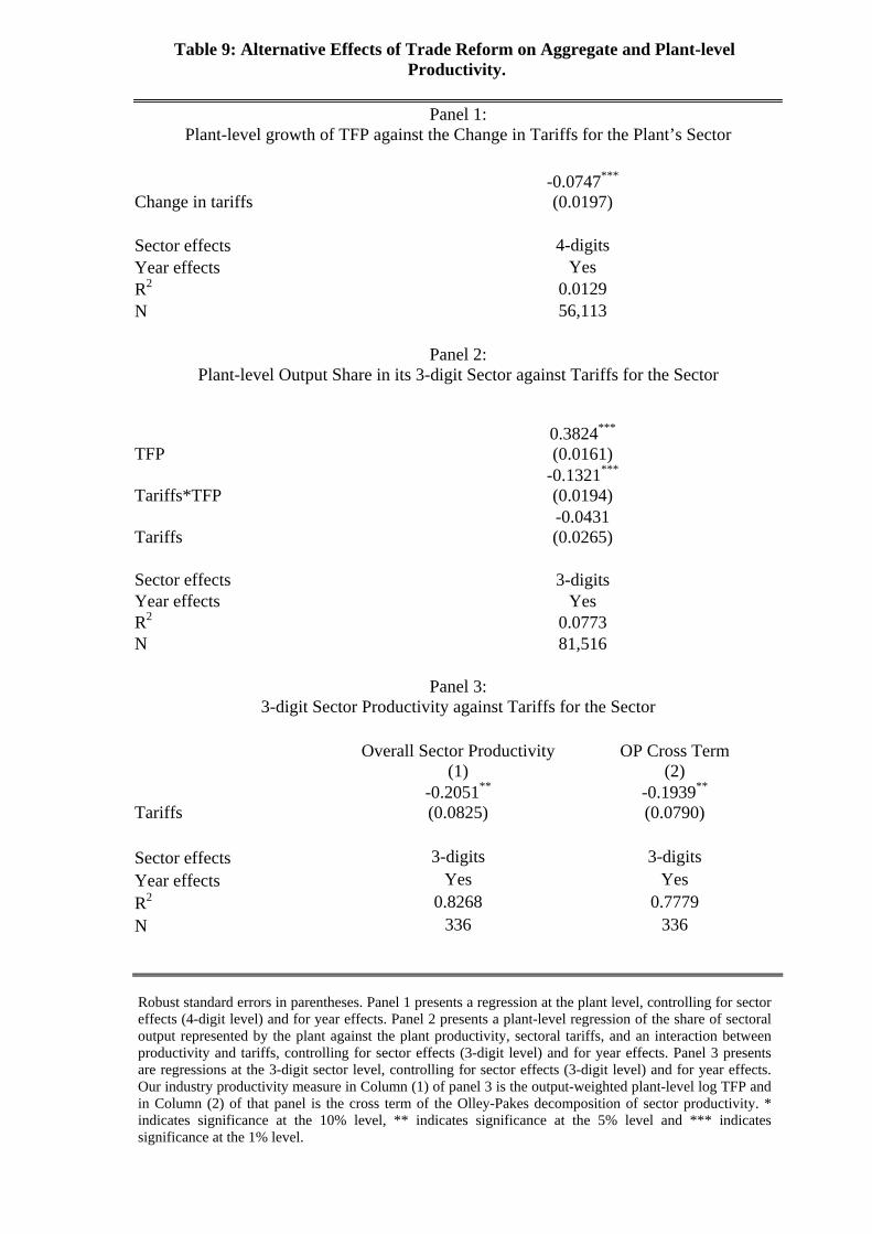
Table 9: Alternative Effects of Trade Reform on Aggregate and Plant-level Productivity.

Panel 1:

Plant-level growth of TFP against the Change in Tariffs for the Plant’s Sector

Change in tariffs -0.0747***

(0.0197) Sector effects 4-digits Year effects Yes R2 0.0129 N 56,113

Panel 2: Plant-level Output Share in its 3-digit Sector against Tariffs for the Sector

TFP 0.3824***

(0.0161)

Tariffs*TFP -0.1321***

(0.0194)

Tariffs -0.0431 (0.0265)

Sector effects 3-digits Year effects Yes R2 0.0773 N 81,516

Panel 3: 3-digit Sector Productivity against Tariffs for the Sector

Overall Sector Productivity

(1) OP Cross Term

(2)

Tariffs -0.2051**

(0.0825) -0.1939**

(0.0790) Sector effects 3-digits 3-digits Year effects Yes Yes R2 0.8268 0.7779 N 336 336

Robust standard errors in parentheses. Panel 1 presents a regression at the plant level, controlling for sector effects (4-digit level) and for year effects. Panel 2 presents a plant-level regression of the share of sectoral output represented by the plant against the plant productivity, sectoral tariffs, and an interaction between productivity and tariffs, controlling for sector effects (3-digit level) and for year effects. Panel 3 presents are regressions at the 3-digit sector level, controlling for sector effects (3-digit level) and for year effects. Our industry productivity measure in Column (1) of panel 3 is the output-weighted plant-level log TFP and in Column (2) of that panel is the cross term of the Olley-Pakes decomposition of sector productivity. * indicates significance at the 10% level, ** indicates significance at the 5% level and *** indicates significance at the 1% level.

Figure 1. Effective tariffs and reform index, 1984-1998

0

0.1

0.2

0.3

0.4

0.5

0.6

0.7

0.8

0.9

1

84 85 86 87 88 89 90 91 92 93 94 95 96 97 98

Year

Effective tariffs St. dev. Effective tariffs Reform Index

Figure 2. Predicted exit probability: actual tariffs vs. 1984 tariffs

0

0.02

0.04

0.06

0.08

0.1

0.12

0.14

85 86 87 88 89 90 91 92 93 94 95 96 97 980

0.002

0.004

0.006

0.008

0.01

0.012

Actual tariffs 1984 tariffs Difference