Tradeoff between the Cycle Complexity and the Fairness of Ring

Tradeoff between the Cycle Complexity and the Fairness of Ring Networks

G. Anastasi•, L. Lenzini•, Y. Ofek*

•University of Pisa, Dept. of Information Engineering

Via Diotisalvi 2 - 56126 Pisa, Italy [email protected], [email protected]

*Synchrodyne

2600 Netherland Ave., Riverdale, NY 10463 [email protected]

Abstract In this paper we study performance tradeoffs of fairness algorithms for ring networks with spatial bandwidth reuse, by using two measures: (i) the fairness cycle size as a complexity measure, and (ii) the Max-Min optimal fairness criterion as a throughput measure. The fairness cycle size is determined by the number of communication links involved in every instance of the fairness algorithm (several identical fairness algorithms can be executed concurrently on the same ring). The study compares three fairness algorithms with different cycle sizes: the Global-cycle algorithm (implemented in the Serial Storage Architecture - SSA) in which the cycle size is equal to the number N of links in the ring; the Variable-cycle algorithm in which its cycle size changes between 1 and N links; the One-cycle, where there is a fairness cycle on every link. It is shown how varying the cycle size affects the network performance with respect to the Max-Min optimal fairness criterion. The results show that for non-homogeneous traffic patterns, decreasing the fairness cycle size, while increasing the complexity, can significantly improve the performance with respect to the Max-Min optimal fairness criterion. Keywords: Ring Networks, Fairness, Cycle Complexity, Max-Min Fairness, SANs.

1 Introduction Ring networks enjoy renewed interest as Storage Area Networks (SANs). A SAN [Phi98] is a high speed

network connecting hundreds of nodes, which are typically disk drives with a storage capacity of up to 10

Gbytes thus providing a total storage capacity in the order of 1012 Bytes. The key emerging storage

technologies are FC-AL (Fiber Channel - Arbitrated Loop, ANSI Standard X3T11) and SSA (Serial

Storage Architecture, ANSI Standard X3T10) [Du98]. SSA is a dual-ring network with spatial bandwidth

reuse in which its underlying network is the MetaRing [Cid93, Che93, and Ofe94].

The main motivation for developing ring networks with spatial bandwidth reuse, such as the MetaRing,

Orwell [Fal85], ATMR [Ohn89] and others, is to increase the aggregate ring throughput, in each direction,

beyond its single link capacity since spatial bandwidth reuse enables concurrent access in each direction of

the ring by more than one node. Increasing the aggregate throughput as much as possible is a key

2

requirement in a SAN environment characterized by the exchange of very large data volumes between

storage devices and their application clients.

DataData

DataData

DataData

DataData

DataData

12

3

4

5

67

8

9

10

1112

Figure 1. Dual-ring with spatial bandwidth reuse

However, using media access such as buffer insertion and slotted ring, in an unregulated manner, may

result in unfair transmission opportunities, and in extreme scenarios it can lead to complete starvation.

Starvation can occur if some nodes are constantly being “covered” by upstream ring traffic, and are thus

not able to access the ring (see Figure 1).

The fairness problem of ring networks with spatial bandwidth reuse has been studied extensively in the

past decade. However, most works have been rather ad-hoc and without objective performance measures.

The objective of this work is thus to study various fairness algorithms for ring networks with spatial

bandwidth reuse by using two measures:

1. Max-Min as an optimal fairness measure of throughput.

2. Fairness cycle size as a space and communication complexity measure.

The performance and complexity measures are introduced in Section 2, while in Section 3 three fairness

algorithms for ring networks, characterized by different cycle sizes, are described. Section 4 defines the

performance metrics of Fairness Deviation and Throughput Deviation. The analysis of the fairness

algorithms is shown in Section 5. Finally, conclusions are drawn in Section 6.

2 Performance and Complexity Measures

2.1 Max-Min Fairness

3

Throughout we will refer to a data exchange between a source node and a destination node as a session.

The Max-Min Fairness definition assumes that each session has a fixed path and that packets are infinitely

small in size (fluid flow model). It is given in terms of session rates [Bert87]. Let sr denote the rate of

session s. Let Cl be the capacity of link l. Furthermore, let Sl be the set of all the sessions using link l, and

Tl denote the sum of rates of all the sessions using link l, i.e., ∈

=lSs

sl rT .

Definition 1: An allocation is said to be feasible if it is 0≥sr for any session s and ll CT ≤ for any link

l.

Definition 2 (Max-Min Fairness): An allocation of a rate rs for session s is Max-Min fair if it is feasible

and for each session s, rs cannot be increased (while maintaining feasibility) without decreasing rs' for

some session s’ for which r rs s' ≤ .

Below it is shown how to compute the Max-Min rates for sessions on a bus- or on a ring-network. The

following procedure is based on [May96, Ber87, Hay81, and Jaf81]:

•= The algorithm maintains a residual capacity for each link, which is initially set to 1.

•= For each session the algorithm associates a label with the possible values assigned or unassigned.

•= All sessions are initially unassigned.

•= The bottleneck-links, in the context of this algorithm, are the links with the smallest residual capacity

per unassigned session sharing them.

•= Computing Max-Min rates:

(1) Find all bottleneck-links.

(2) Divide the residual capacity of a bottleneck link by the number of its unassigned sessions. Assign

this as the Max-Min fair rate of those sessions and label them assigned.

(3) Compute the residue capacity of all links by subtracting the rates which have been assigned to

sessions in step (2). Repeat 1-3 until all sessions are assigned.

4

For a simple example on how Max-Min fair rates are computed, consider Figure 2. The labels A through

H represent network nodes, which are sources of sessions along a bus network. All session flows are from

left to right and are named after their sources. The feasibility condition is that for each link the sum of the

rates allocated to sessions sharing that link should not exceed 1.

A Max-Min fair rates allocation in this example is as follows:

r r rA B C= = =13 ,

41==== HGFE rrrr , and rD = − =1

13

23

, where ri is the rate of session i.

To see why, we follow the above algorithm. Initially, the bottleneck is created by the traffic from

{E,F,G,H}, and therefore, each of those sessions gets a rate of 1/4, and on the respective links these rates

are subtracted from 1 to acquire the new residual capacity. After that, the bottleneck is created by the

traffic from {A, B, C}, and therefore, each of those sessions acquires a rate of 1/3; and on the respective

links these rates are subtracted from 1 to get the new residual capacity. Then, since only session D is

unassigned, because it has the residual capacity of 2/3 on its links, it will get all of it.

A GB C D E F

Bottleneckof size 3

Bottleneckof size 4

H

Figure 2. Multiple sessions on a bus segment

2.2 Fairness cycle size The aim of a fairness algorithm is to regulate the access to the ring such that all nodes have an opportunity

to access the ring. The simplest form of such fairness is round robin, used in token ring [Far69, Bux83,

and Ros86], in which each node gets its turn to transmit in a cyclical order. In round robin fairness a node

gets its turn to transmit after all the other N-1 nodes have had a chance to transmit. In ring networks with

spatial bandwidth reuse round robin fairness cannot be used. However, the notion of cycle can still be used

for fairness. Thus, in this paper the fairness cycle size is used to characterize fairness algorithms.

5

Definition 3: The fairness cycle size is defined as the number of links used in order to determine when a

node can get another transmission opportunity.

According to the above definition, in round robin fairness the cycle size is equal to the number of links in

the ring, i.e., N. In general, the following cases can be distinguished:

−= global-cycle: the cycle size is equal to the number of links in the ring – N (as in round robin). This

means that only one instance of the fairness algorithm is executed over the ring at any given time. A

global-cycle algorithm views each direction of the ring as a single shared communication resource.

The objective of such an algorithm is to ensure that all nodes have an equal opportunity to access the

network.

−= variable-cycle: the cycle size changes between 1 and N links. This implies that between N and 1

instances of the fairness algorithm are executed at any given time. Unlike to global cycle algorithms,

variable cycle algorithms view each link as a single communication resource and the whole ring as a

multiplicity of communication resources.

−= one-cycle: there is a fairness cycle for every link. This implies that N instances of the fairness

algorithm are executed at any given time - one for each communication link.

Communication/Hardware complexity

global-cycle O(1) variable-cycle For ring O(lg N)

For bus O(1) one-cycle O(N)

Table 1. Complexity Measures of the Fairness Algorithms

The complexity associated with each of the algorithm types is summarized in Table 1. A global-cycle

algorithm requires the exchange of only one bit of information, as shown in Section 3.2. A variable-cycle

algorithm requires the use of the node ID, and therefore, in a ring of N nodes the complexity is O(lg N) as

shown in Section 3.3. However, if it is a bus the complexity is only O(1) since there is no need for an ID.

A one-cycle algorithm requires that every ring interface will maintain a table with an entry to all other

nodes, and the control messages are bit-vectors of size N (for a ring with N links), and therefore, the

6

complexity of this algorithm is O(N), as shown in Section 3.4.

3 Fairness Algorithms for Ring Networks In this section we briefly describe three fairness algorithms designed for ring networks with spatial

bandwidth reuse and characterized by different cycle sizes. To emphasize this aspect in the following we

will refer to these algorithms as the Global-cycle algorithm, the Variable-cycle algorithm and the One-

cycle algorithm, respectively.

3.1 Network model We consider a dual ring network with N nodes and assume that the transmission time around the ring is

divided into time slots of equal duration. Each slot starts with a busy-bit; if this bit is 0, the slot is empty,

otherwise the slot is full. A node can transmit a packet only if it receives an empty slot. The packet is

removed from the ring by its destination node and the slot becomes empty. The shortest path criterion is

used for packet routing, i.e., to choose one of the two possible directions (rings) toward the final

destination.

In the description of the algorithms the concept of Quota, q, will used extensively. It denotes a predefined

number of transmission permits. Each permit is used by a node to access one empty slot.

3.2 Global-cycle Fairness Algorithm In order to achieve fairness, the Global-cycle algorithm regulates access to each direction of the ring by

means of a control signal, called SAT (from SATisfied), which circulates in the same or opposite direction

to the data traffic it regulates, see Figure 3 and [Cid93, Ofe94] for details.

In principle, the node forwards the SAT signal upstream without any delay, unless it is not SATisfied or

“starved.” By “starved” we mean that the node has been unable to use the permitted number of slots since

the last time it forwarded the SAT signal. Specifically, the node is SATisfied if between two consecutive

visits of the SAT signal, the node has used q slots or if its output buffer is empty. If the node is not

SATisfied, it will hold the SAT until it is SATisfied and then forward the SAT upstream. After a node

forwards the SAT, it can use up to q more slots, before receiving and forwarding the SAT signal again.

7

OutputBuffer

InputBuffer

RR TT

Node 2Node 2

OutputBuffer

InputBuffer

RR TT

Node 1Node 1

Slot k-2Slot k-2

Slot k+1Slot k+1

Slot k-3Slot k-3Slot kSlot kSlot k-1Slot k-1

Slot k+2Slot k+2

SAT Signal

Figure 3. Global-cycle fairness with the SAT signal

3.3 Variable-cycle Fairness Algorithm The Variable-cycle algorithm [Che93] has two modes of operation: (1) unrestricted and (2) restricted.

Initially, a node is unrestricted and can transmit whenever it encounters an empty slot. This mode is

identified as the Free Access (FA) state, shown in Figure 4. A node will enter the restricted mode if it

cannot transmit (does not encounter empty slots) or if it receives a signal from a downstream node that

cannot transmit. The restricted mode has three states: Tail (T), Body (B) and Head (H), shown in Figure 4.

In the restricted mode a node can transmit only a predefined Quota, q, before it transits back to the non-

restricted mode.

T

FAB

H

R_REQ/

R_GNT/

Starvation/S_REQ

SATisfied/ S_GNT

R_REQ/

R_GNT/No empty slots/S_REQ

Figure 4. Variable-cycle fairness state transition diagram

The algorithm uses two control signals to facilitate the transition between the states and operation modes,

as shown in Figure 5:

REQ: This signal initiates the restricted period of operation and is forwarded upstream over the

congested ring segment.

8

GNT: This signal is used, when the node is satisfied, to terminate the local fairness cycle.

The two control signals create fairness cycles over the congested segments of the ring. Note that if the ring

is congested, the time interval a node is in the non-restricted mode can be zero. In this case, a node will

transmit one Quota in every fairness cycle. The size of a fairness cycle depends on the number of nodes

this node is interfering with, directly and indirectly. For example, if node A interferes with node B, and

node B interferes with node C, then node A also interferes with node C (i.e., the interference is a transitive

closure operation).

A starved node triggers a fairness cycle by sending the REQ signal upstream and by entering the tail (T)

State. Upon reception of the REQ signal, a node enters the restricted mode of operation, and if its

upstream is idle, it will enter the head (H) State. If this node cannot provide empty slots downstream, it

will forward the REQ upstream, and will enter the body (B) state. Upon satisfaction, i.e., transmission of a

Quota of q slots, the tail node sends a GNT signal upstream and transits back to the non-restricted free

access (FA) state. Upon receiving this GNT, the node upstream follows similar rules: if it is in the body

node, it transits to a tail (T) state and will similarly forward GNT upon satisfaction; if it is in the Head

State, the local fairness cycle on this segment of the ring is terminated.

REQREQ Node k+1

Node k

Node k+3

Node k+2

GNTGNTT

BB

B

H

REQREQREQREQ

REQREQ

GNTGNT

Figure 5. Variable-cycle REQUEST PATH (from Node k+3 to Node k+1)

In this scenario, the algorithm has created a REQUEST PATH, which contains unique and distinct head

and tail nodes. Each node of the REQUEST PATH is able to transmit one Quota including the tail

initiator, as shown in Figure 5.

It can be easily verified that the following properties hold

9

•= The size of the fairness cycle, which is the size of the REQUEST PATH, varies between 1 and N.

•= In every cycle each node in the REQUEST PATH can transmit one Quota.

•= However, nodes on different REQUEST PATHs can transmit different numbers of Quotas.

3.4 One-cycle Fairness Algorithm In the One-cycle algorithm [May96] every node i maintains a table with an entry for every other node.

Each entry j reflects the status of node i with respect to node j, if node j is the source of a conflicting

downstream session. Hence, a source which sends packets through node i can be uniquely labeled

“upstream” with respect to node i, thus “upstream” and “downstream” are always well defined.

The table is denoted "mode" and each entry mode[j] has a value in the set:

Unregulated - implies that node i can transmit through node j “freely”.

Regulated - implies that node i can only transmit one more Quota before it becomes exhausted with

respect to node j.

Exhausted - implies that node i can no longer send any packets through node j. Consequently, if a node

wants to transmit a new Quota, it has to check that all entries of conflicting downstream nodes are not

exhausted.

ExhaustedB

RegulatedC

IrrelevantD

IrrelevantE

IrrelevantF

IrrelevantG

IrrelevantH

Figure 6. Table "Mode" for Node A in Figure 2

For the example shown in Figure 2, a possible value of the table of node A is shown in Figure 6. If node A

wants to transmit a new Quota, it has to check the entries of nodes B and C, since these are the conflicting

downstream sessions. As it turns out, the entry of node B is exhausted and hence node A cannot transmit

10

right away.

The table mode is updated by the following two control-signals:

R(j) - which indicates that node j wants to start transmitting another Quota, and

U(j) - which indicates that node j just finished transmitting a Quota.

If active node i receives an R-signal from a conflicting node j (session) downstream, i knows that a new

conflict has arisen with j, and hence sets mode(j) to regulated. Likewise, if i receives a U-signal from node

j, i knows that the current conflict has ended and it sets mode(j) to unregulated. If node i is conflicting

with downstream node j and mode(j) is set to regulated, then after transmitting one Quota, mode(j) is set

to exhausted. These simple state transitions are shown in Figure 7.

Unregulated

Exhausted Regulated

Receipt of R(j)

Receipt of U(j)Receipt of U(j)

Finish sending one quota through j

Transmit quotas

Transmit a quota

Figure 7. State diagram for Mode(j) at Node i

When node i tries to transmit a new Quota, it checks its table and if it is positive (i.e., all conflicting

downstream nodes are not exhausted), then node i sends an R(i)-signal upstream to indicate to conflicting

upstream nodes that a new cycle is about to start. Subsequently, node i transmits q packets in q empty

slots. After finishing one Quota (or after ceasing to be active), node i sends an U(i)-signal upstream to

indicate to upstream nodes that the current cycle of conflict has ended. It then updates its table according

to the state-transition diagram in Figure 7 and the signals it received from downstream nodes.

4 Performance Metrics In this section we will define some indices on which the performance analysis reported in the next section

will be based. Throughout we will refer to γ= i as the throughput achieved by node i normalized to the ring

capacity. Specifically, γ= i is defined as:

11

( )

si

i tT

TN=γ

where ( )TNi indicates the number of packets transmitted by node i in a time interval of duration equal

to T time slots, and st is the time needed to transmit a packet (i.e., the slot duration). Hence, st is the

inverse of the link capacity expressed in slots/second.

Having defined the normalized node throughput we are now in a position to define the Fairness Deviation

index. For a given fairness algorithm, if N is the number of nodes in the ring, the Fairness Deviation Fδ

is defined as:

2

1=

��

� −=N

ioi

oi

fai

F γγγδ [1]

In [1], faiγ is the throughput achieved by node i when a given fairness algorithm is used, while o

iγ is the

optimal throughput for node i calculated according to the Max-Min definition (see Definition 2 and

related references). For a given algorithm, the Fairness Deviation provides a measure of the algorithm's

effectiveness, i.e., how much the fairness provided by the algorithm deviates from the optimal fairness

definition.

However, another important issue in the evaluation of a fairness algorithm is the algorithm's efficiency,

i.e., how close the aggregate (normalized) throughput provided by the algorithm is to the optimal

aggregate (normalized) throughput. To measure the algorithm’s efficiency, the Throughput Deviation

index will be used. For a given fairness algorithm, if N is the number of nodes in the ring, the

Throughput Deviation Tδ is defined as:

=

==

−= N

i

oi

N

i

oi

N

i

fai

T

1

11

γ

γγδ [2]

12

As can be seen, Tδ is the difference between the aggregate (normalized) throughput provided by a

specific fairness algorithm and the optimal aggregate (normalized) throughput, normalized to the optimal

aggregate (normalized) throughput. By definition, Tδ is positive if the fairness algorithm provides, for a

specific traffic scenario, an aggregate throughput greater than the optimal aggregate throughput, and

negative otherwise.

We will refer to an ideal fairness algorithm as the algorithm for which both Fairness and Throughput

Deviations are equal to zero. By definition, 0 0 == TF δδ . On the other hand, the reverse implication

does not usually hold.

5 Analysis of Fairness Algorithms To assess the fairness algorithms introduced in Section 3 we assume that nodes in the ring are equally

spaced and each of them operates in never empty queue conditions, i.e., each node always has packets to

send. Furthermore, we assume that each node sends packets to a unique fixed destination. Under this

assumption the resulting traffic scenario is static and, hence, the Max-Min definition and the algorithm

reported in Section 2.1 can be used to compute Max-Min rate of sessions, i.e., the optimal throughput

achievable by network nodes. This allows us to assess how close to the Max-Min Fairness each of the

above fairness algorithms operates. To this end, we need to consider some traffic scenarios and, hence, we

have to decide how to select these traffic scenarios.

5.1 Traffic Scenarios The number of potential traffic scenarios is very large and exponentially increases with the number, N ,

of nodes attached to the network and, hence, an exhaustive analysis of traffic scenarios is impractical.

Therefore, in our analysis we focus on some specific scenarios, which are of special interest. The

scenarios are selected according to some general principles, which are introduced below. Network

scenarios can be distinguished into the following three classes.

1. Class 1 scenarios - disjoint groups and homogeneous workloads. Nodes in the ring are divided into

13

disjoint groups and each node within a group only transmits to the last node in its group. Furthermore,

all the groups have the same number of nodes and, hence, the workload is homogeneously distributed

between the groups. Scenarios conforming to this principle (see, for example, Figure 8), will be

referred to throughout as Class 1 scenarios. All three fairness algorithms are expected to perform

similarly for this class of idealized, symmetric, and homogeneous traffic scenarios.

2. Class 2 scenarios - disjoint groups and non-homogeneous workloads. The only difference with

respect to Class 1 scenarios is that the number of nodes varies from group to group (see, for example,

Figure 12). Hence, the workload is now non-homogeneously distributed between groups. It is

expected that the Variable-cycle and One-cycle algorithms will perform better than the Global-cycle

algorithm, since the former two fairness algorithms work within each group without affecting the

performance of nodes belonging to other groups. Hence, scenarios conforming to the above principle,

hereafter Class 2 scenarios, should highlight the non-ideal ( Tδ and Fδ different from zero) behavior

of the Global-cycle fairness algorithm.

3. Class 3 scenarios - non-disjoint groups and non-homogeneous workloads. In this case the traffic

from one group covers nodes on the other group downstream and the group size varies (see, for

example, Figure 16). Scenarios conforming to this principle will be referred to throughout as Class 3

scenarios. Since groups are now non-disjoint it is expected that for this class of scenarios the

Variable-cycle fairness algorithm will perform similarly to the Global-cycle fairness algorithm, since

the request path, defined in Figure 5, can cover the whole ring.

In the following two subsections we will derive analytical expressions for Fδ and Tδ for Class 1 and

Class 2 scenarios. Scenarios belonging to Class 3 are characterized by more complicated inter-

dependencies between network nodes which make the analytical tractability very difficult if not

impossible. Hence, for Class 3, Fδ and Tδ values reported below (see Section 5.4) were obtained by

simulation.

14

5.2 Analytical Results for Class 1 Scenarios In deriving analytical expressions for Fδ and Tδ the following notations are used:

•= G is the number of disjoint groups of nodes in the ring.

•= gN is the number of transmitting nodes1 in group Ggg ,...,2,1 , = .

•= S is the ring size (in slots).

•= d is the distance (in slots) between two consecutive nodes.

Throughout, we will assume that the value of q (i.e., the Quota) is the same for all nodes in the ring and

for all three fairness algorithms. Furthermore, in the Variable-cycle algorithm a node will be assumed as

starved if it has observed a number of consecutive busy slots greater than a predefined “starvation Quota”

denoted throughout by sq .

Before deriving analytical expressions for Fδ and Tδ it is worthwhile to remember that Class 1 scenarios

are characterized by an equal number of (transmitting) nodes EN in every group, i.e., Eg NN = for any

g.

MAX-MIN RATES In a Class 1 scenario the number of bottlenecks is equal to the number of disjoint groups, and the

bottlenecks have the same size, EN . Hence, by using the algorithm described in Section 2.1 it can be

easily verified that the Max-Min rate of node i ( ENi ,...2,1= ) in group ( )Ggg ,...,2,1 = is:

EE

oi Ni

N,...,2,1 1 ==γ [3]

and the aggregate (normalized) throughput for Class 1 scenarios is equal to the number of disjoint groups

in the network, i.e.,

1 By definition,

gN does not include the common destination node.

15

GN

G

g

N

j E

N

i

oi

E

= ==

==1 11

1γ [4]

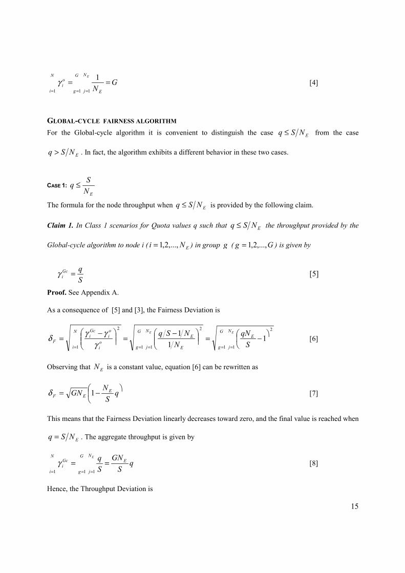
GLOBAL-CYCLE FAIRNESS ALGORITHM For the Global-cycle algorithm it is convenient to distinguish the case ENSq ≤ from the case

ENSq > . In fact, the algorithm exhibits a different behavior in these two cases.

CASE 1: EN

Sq ≤

The formula for the node throughput when ENSq ≤ is provided by the following claim.

Claim 1. In Class 1 scenarios for Quota values q such that ENSq ≤ the throughput provided by the

Global-cycle algorithm to node i ( ENi ,...,2,1= ) in group g ( Gg ,...,2,1= ) is given by

SqGc

i =γ

[5]

Proof. See Appendix A.

As a consequence of [5] and [3], the Fairness Deviation is

= == ==

��

� −=��

��

� −=�

��

��

� −=

G

g

N

j

EG

g

N

j E

EN

ioi

oi

Gci

F

EE

SqN

NNSq

1 1

2

1 1

2

1

2

11

1γ

γγδ [6]

Observing that EN is a constant value, equation [6] can be rewritten as

��

� −= qS

NGN EEF 1δ [7]

This means that the Fairness Deviation linearly decreases toward zero, and the final value is reached when

ENSq = . The aggregate throughput is given by

qS

GNSq E

G

g

N

j

N

i

Gci

E

=== == 1 11

γ [8]

Hence, the Throughput Deviation is

16

1−=−

= qS

NG

GqS

GNE

E

Tδ [9]

Like Fδ , Tδ exhibits a linear behavior. Specifically, the Throughput Deviation increases toward zero as q

increases. Again, the final value is reached for ENSq = .

CASE 2: EN

Sq >

For q values such that ENSq > the formula for the node throughput is provided by Claim 2 below.

Claim 2. In Class 1 scenarios for Quota values q such that ENSq > the throughput provided by the

Global-cycle algorithm to node i (for ENi ,...,2,1= ) in group g ( Gg ,...,2,1= ) is given by

E

Gci N

1=γ [10]

Proof. See Appendix A.

Equation [10] implies that, in Class 1 scenarios, when ENSq > the Global-cycle algorithm behaves

ideally, i.e., 0=Fδ and 0=Tδ .

VARIABLE-CYCLE ALGORITHM The formula for node throughput offered by the Variable-cycle algorithm in Class 1 scenarios is provided

by the following

Claim 3. In Class 1 scenarios the throughput provided by the Variable-cycle algorithm to node i (for

gNi ,...,2,1= ) in group g ( Gg ,...,2,1= ) is given by

�

�

�

==+++

+

=+++

+++

=

Egsgg

sgg

s

Vci

NNiifqdNqN

dq

iifqdNqN

qdq

,...3,2 12

2

1 12

12

γ [11]

17

Proof. In [Ana96] it is proved that formula [11] provides the node throughput when the ring includes a

single group of nodes where each node transmits to the last node in the group. It is easy to prove that the

same formula can be extended to scenarios with more than one group provided that (i) groups are disjoint;

and (ii) all the nodes in each group transmit to the last node in the same group. In fact, since groups are

disjoint, Request Paths span, at most, a single group. Hence, the behavior of each node is influenced by

the other nodes in the same group but does not depend at all on nodes belonging to different groups. In

conclusion, each group can be considered in isolation, and the formula derived in [Ana96] can thus be

used. Since Class 1 (and Class 2) scenarios satisfy conditions (i) and (ii) the claim is proved. �

From [11] the following considerations can be drawn. The aggregate throughput within each (disjoint)

group is equal to 1. Hence, the aggregate throughput is equal to the number of disjoint groups G, and the

Throughput Deviation Tδ is equal to zero for any value of parameters q, sq , gN and d .

Furthermore, [11] clearly shows that the first node in each group has an advantage over the other ones.

However, it can also be observed that when q approaches infinity the algorithm asymptotically tends to

provide the same throughput ( Eg NN 11 = ) to all nodes. In fact, in [11], for i=1, as q gets larger the

contribution of the term 1+sq becomes negligible with respect to the quantity dq 2+ .

The expression for Fδ can be easily obtained by introducing the node throughputs specified by [11] into

[1]. The above remarks imply that the Fairness Deviation asymptotically decreases toward zero when the

Quota approaches infinity, i.e., the Variable-cycle algorithm tends to become optimal even in terms of

Fairness as the Quota becomes larger and larger.

ONE-CYCLE ALGORITHM The behavior of the One-cycle algorithm is much more complex to analyze than the Variable-cycle and

the Global-cycle algorithms. A closed formula like [11] is difficult, if not impossible, to obtain since δF

and δT generally depend on the particular value of q that is used. In principle, once this value has been

18

fixed, node throughputs and, hence, δF and δT could be derived graphically. However, this procedure is

complex. Furthermore, the system behavior depends on the value of q. Therefore, the only reasonable way

for computing δF and δT is by simulation.

5.3 Analytical Results for Class 2 Scenarios

MAX-MIN RATES In Class 2 scenarios there are as many bottleneck links as disjoint groups but, unlike Class 1 scenarios,

bottlenecks have different sizes. In fact, the bottleneck size is determined by the number of sending nodes

in the corresponding group. By using the algorithm described in Section 2.1 it is easy to verify that the

Max-Min rate related to node i ( gNi ,...2,1= ) in group ( )Ggg ,...,2,1 = is

GgNiN g

g

oi ,...,2,1;,...,2,1 1 ===γ

The difference from Class 1 scenarios is that gN is no longer a constant and, hence, nodes in different

groups are characterized by different rates. However, as for Class 1 scenarios, the aggregate (normalized)

throughput is equal to the number G of disjoint groups in the ring.

GLOBAL-CYCLE FAIRNESS ALGORITHM As for Class 1 scenarios the node throughput provided by the Global-cycle algorithm is expressed by two

different formulas depending upon MNSq ≤ or MNSq > , where ( )ggM NmaxN = . Hence, the two

cases are considered separately below.

Case 1: MN

Sq ≤

The formula to be used when MNSq ≤ is provided by the following:

Claim 4. In Class 2 scenarios for Quota values q such that MNSq ≤ the throughput provided by the

19

Global-cycle algorithm to node i ( gNi ,...,2,1= ) in group g ( Gg ,...,2,1= ) is

SqGc

i =γ [12]

Proof. See Appendix B.

From [12] it follows

== ==

��

�−=

��

��

�

� −=�

��

��

� −=

G

g

gg

G

g

N

j g

gN

ioi

oi

Gci

F SqN

NN

NSqg

1

2

1 1

2

1

2

11

1γ

γγδ [13]

Furthermore, the aggregate throughput is

SqN

Sq G

gg

G

g

N

j

N

i

Gci

g ��

�==

== == 11 11γ

[14]

and, hence, the analytical expression for the Throughput Deviation is

1111

−�

��

�=

�

��

�−

��

�=

== SGqNG

SqN

G

G

gg

G

ggTδ

[15]

Case 2: MN

Sq >

In this case the following Claim can be exploited:

Claim 5. In Class 2 scenarios for Quota values q such that MNSq > the throughput provided by the

Global-cycle algorithm node i ( gNi ,...,2,1= ) in group g ( Gg ,...,2,1= ) is equal to

M

Gci N

1=γ [16]

Proof. See Appendix B. From [16], after some algebraic manipulations it follows

=

��

�−=

G

g M

ggF N

NN

1

2

1δ [17]

20

Hence, the Fairness Deviation is constant and only depends on the number of nodes in each group.

From [16] it can be easily verified that the Throughput Deviation is

��

�−=

=

G

g M

gT G

NN

G 1

1δ [18]

This means that the Throughput Deviation is a constant whose value is always negative unless Mg NN =

for any g , i.e., unless gN is constant. In the latter case a Class 2 scenario degenerates into a Class 1

scenario and, in fact , Tδ becomes equal to zero.

VARIABLE-CYCLE FAIRNESS ALGORITHM Claim 6. In Class 2 scenarios the throughput provided by the Variable-cycle algorithm to node i (for

gNi ,...,2,1= ) in group g ( Gg ,...,2,1= ) is

�

�

�

=+++

+

=+++

+++

=

gsgg

sgg

s

Vci

NiifqdNqN

dq

iifqdNqN

qdq

,...3,2 12

2

1 12

12

γ

Proof. See the proof of Claim 3.

Since the formula for the node throughput is the same as for Class 1 scenarios, the remarks on Fδ and Tδ

reported in Section 5.2 apply to Class 2 scenarios as well.

ONE-CYCLE FAIRNESS ALGORITHM As for Class 1 scenarios a closed formula for the One-cycle algorithm is very difficult to obtain, if not

impossible, and simulation thus seems to be the only viable solution.

5.4 Comparative Assessment of the Algorithms This section compares the Fairness and Throughput Deviations of the proposed fairness algorithms as a

21

function of the Quota (q) by considering a particular scenario for each class defined in Section 5.1. In all

the scenarios taken into consideration the number of nodes, N, is equal to 12.

However, analytical results are only available for scenarios belonging to Class 1 and Class 2, and even for

these classes they only refer to the Global-cycle and Variable-cycle algorithms. Therefore, to make the

analysis as complete and meaningful as possible, we used computer simulation for those cases for which

analytical results were not available1. Specifically, for each scenario, we considered three different values

for the distance between nodes (i.e., d=1/12, 1 and 10 slots) and consequently, three different ring sizes

(i.e., 1, 12 and 120 slots).

The performance of the three algorithms in the selected scenarios is discussed in the following subsections

(5.4.1 - 5.4.3). The results shown in subsections 5.4.1 and 5.4.2 were obtained partly by the analytical

formulas derived in sections 5.2 and 5.3 (Global-cycle and Variable-cycle for d=1 and d=10) and partly by

simulation (d=1/12). On the other hand, the results presented in subsection 5.4.3 were derived by

simulation.

5.4.1 Scenario 1: Disjoint Groups and Homogeneous Workload We started our analysis by considering the traffic Scenario 1, depicted in Figure 8, which belongs to Class

1. Figures 9, 10 and 11 show the Fairness and Throughput Deviations as a function of the Quota q for

different ring sizes (e.g., d values). In each figure the Fairness Deviation is reported in the left hand plot

while the Throughput Deviation is shown in the right hand plot.

A comparison of Figures 9, 10 and 11, clearly shows that in this scenario all three fairness algorithms

behave ideally when the value of q is greater than a certain threshold whose value, for each algorithm, is

reported in Table 2. Specifically, an infinite threshold value for the Variable-cycle algorithm means that

the algorithm asymptotically tends to an ideal behavior.

1 All the simulation results presented in this paper have been estimated by using the independent replication method and assuming a confidence level of 90% [Law82]. The duration of each simulation experiment was fixed in such a way as to achieve confidence intervals less than 5 %.

22

121

2

3

456

78

9

10

11

Figure 8. Traffic Scenario 1

0

0.5

1

1.5

2

2.5

3

0 5 10 15 20 25

Scenario 1; d=1/N

One-cycleVariable-cycleGlobal-cycle

Fairn

ess D

eviat

ion

q

-1

-0.8

-0.6

-0.4

-0.2

0

0 5 10 15 20 25

Scenario 1; d=1/N


Thro

ughp

ut De

viatio

n

q

Figure 9. Fairness and Throughput Deviations for Scenario 1 when d=1/N

0

0.5

1

1.5

2

2.5

3

0 10 20 30 40 50

Scenario 1; d=1


Fairn

ess D

eviat

ion

q

-1

-0.8

-0.6

-0.4

-0.2

0

0 10 20 30 40 50

Scenario 1; d=1


Thro

ughp

ut De

viatio

n

q

Figure 10. Fairness and Throughput Deviations for Scenario 1 when d=1

23

The threshold values and the behavior of the Global-cycle and Variable-cycle algorithms can be justified

on the basis of the considerations reported in Section 5.2. Specifically, the ideal behavior is a consequence

of the same number of nodes in each disjoint group.

For the One-cycle algorithm the non-ideal behavior of the Fairness Deviation when the value of q is less

than or equal to 2d (i.e., twice the delay time between nodes) can be explained as follows. Due to the

propagation delay the control signals R() and U() used by the algorithm take a delay time of d slots to go

from a node to the neighbor upstream node. This causes an imbalance in the number of quotas transmitted

by each nodes.

For example, after sending a quota of packets a generic node i sends the U(i) signal to the upstream nodes.

Due to the propagation delay the U(i) signal reaches the closest upstream node after d slots and, hence,

node i has the opportunity to transmit up to 2d additional packets (unless it is restricted by downstream

competing nodes)1 before being covered by the upstream traffic. This implies that, when the quota value is

less than or equal to 2d, some node may transmit more quotas than others. The imbalance in the number of

quotas transmitted by each node actually depends on the value of q (and this justifies the discontinuous

behavior of the curve). When the quota value is greater than 2d a node can never complete a new quota

after sending the U() signal upstream, and, in conclusion, all nodes transmit the same number of quotas.

From Figures 9-11 it also appears that both the Variable-cycle and the One-cycle algorithms exhibit a

Throughput Deviation δT, which is equal to zero for any q value. From a practical point of view, this result

is a consequence of the property by which, at any time, there is at least one transmitting node in the ring.

This property does not hold for the Global-cycle algorithm for any value of q. In fact, for the latter

algorithm the Throughput Deviation is negative for ENSq < .

1 Please note that nodes 3, 7 and 11 in Figure 8 are never restricted.

24

0

0.5

1

1.5

2

2.5

3

0 10 20 30 40 50

Scenaro 1; d=10


Fairn

ess D

eviat

ion

q

-1

-0.8

-0.6

-0.4

-0.2

0

0 10 20 30 40 50

Scenario 1; d=10


Thro

ughp

ut De

viatio

n

q


Fairness Algorithm

Threshold

Value

One-cycle 2d

Variable-cycle ∞=

Global-cycle S/NE

Table 2. Values of q after which the three Fairness Algorithms behave ideally

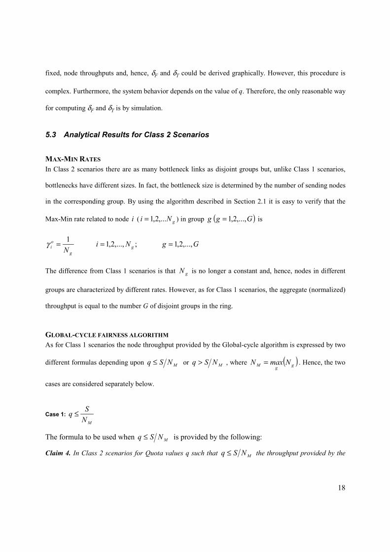
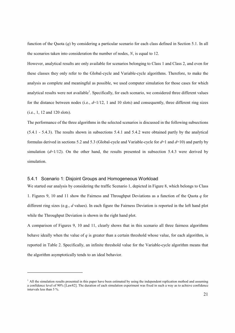
5.4.2 Scenario 2: Disjoint Groups and Non-Homogeneous Workload The next step in our analysis is to show how the Global-cycle algorithm “breaks” in a Class 2 scenario like

the one shown in Figure 12, hereafter referred to as Scenario 2. In Scenario 2 there are three disjoint

groups with different numbers of nodes and, hence, three bottlenecks of different sizes: 2, 3 and 4

respectively.

Fairness and Throughput Deviations for the three ring sizes taken into consideration are reported in

Figures 13, 14 and 15. By comparing Figures 13-15 with the corresponding figures related to the previous

scenario (9-11) we can see that there is no difference as far as the Variable-cycle and One-cycle

algorithms are concerned. Specifically, the One-cycle algorithm behaves ideally when the value of q is

greater than d2 (the reasons for the non-ideal and discontinuous behavior when dq 2≤ are the same as

in Section 5.4.1) while the Variable-cycle asymptotically tends to be ideal as the value of q increases.

25

121

2

3

456

78

9

10

11


0

0.5

1

1.5

2

2.5

3

0 5 10 15 20 25

Scenario 2; d=1/N


Fairn

ess D

eviat

ion

q

-1

-0.8

-0.6

-0.4

-0.2

0

0 5 10 15 20 25

Scenario 2; d=1/N


Thro

ughp

ut De

viatio

n

q

Figure 13. Fairness and Throughput Deviations for Scenario 2 and d=1/N

On the other hand, the behavior of the Global-cycle algorithm is noticeably different from the previous

scenario. In fact, it is no longer Max-Min fair even for large values of q (see [17] and [18]). This is due to

the non-homogeneous distribution of the workload between groups, which implies bottlenecks of different

sizes. The Global-cycle algorithm provides all the nodes with the same throughput - determined by the

bottleneck with the largest size - hence, degrading the performance of nodes belonging to groups with a

small number of competing nodes. As a consequence, both the Fairness and Throughput Deviations

cannot be null.

26

0

0.5

1

1.5

2

2.5

3

0 10 20 30 40 50

Scenario 2; d=1


Fairn

ess D

eviat

ion

q

-1

-0.8

-0.6

-0.4

-0.2

0

0 10 20 30 40 50

Scenario 2; d=1


Thro

ughp

ut De

viatio

n

q


0

0.5

1

1.5

2

2.5

3

0 10 20 30 40 50

Scenario 2; d=10


Fairn

ess D

eviat

ion

q

-1

-0.8

-0.6

-0.4

-0.2

0

0 10 20 30 40 50

Scenario 2; d=10


Thro

ughp

ut De

viatio

n

q


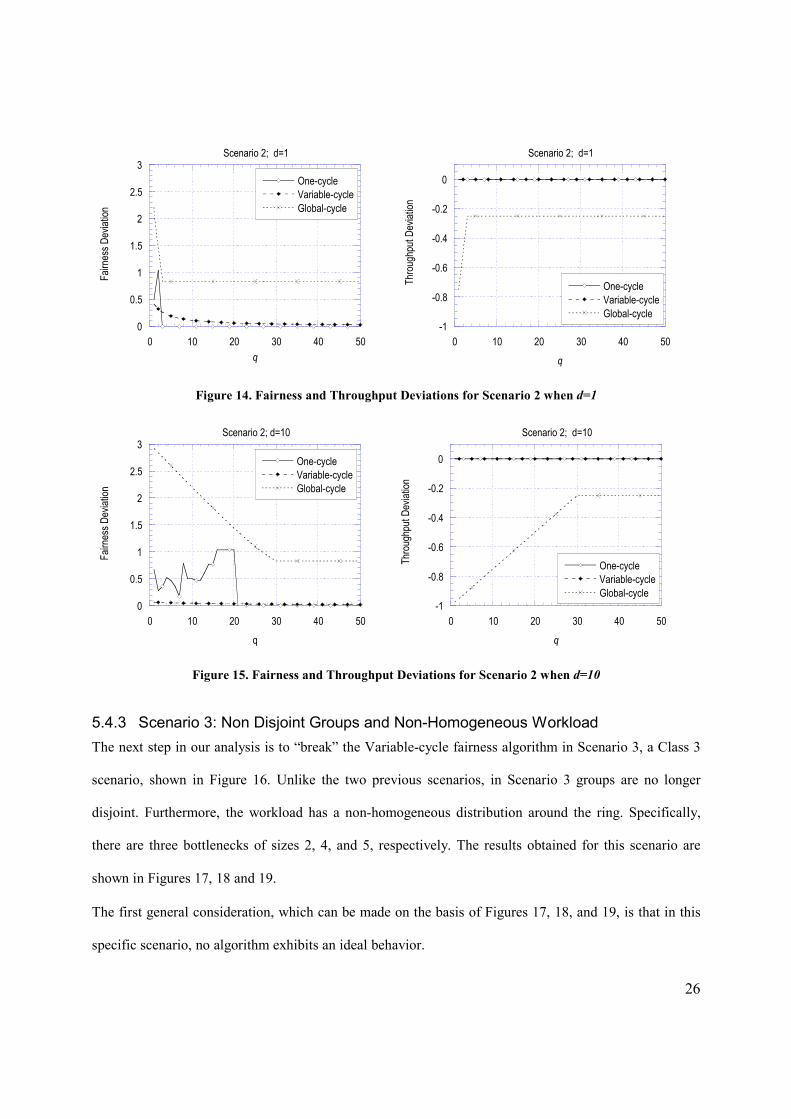
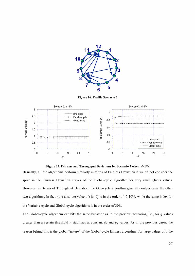
5.4.3 Scenario 3: Non Disjoint Groups and Non-Homogeneous Workload The next step in our analysis is to “break” the Variable-cycle fairness algorithm in Scenario 3, a Class 3

scenario, shown in Figure 16. Unlike the two previous scenarios, in Scenario 3 groups are no longer

disjoint. Furthermore, the workload has a non-homogeneous distribution around the ring. Specifically,

there are three bottlenecks of sizes 2, 4, and 5, respectively. The results obtained for this scenario are

shown in Figures 17, 18 and 19.

The first general consideration, which can be made on the basis of Figures 17, 18, and 19, is that in this

specific scenario, no algorithm exhibits an ideal behavior.

27

121

2

3

456

78

9

10

11


0

0.5

1

1.5

2

2.5

3

0 5 10 15 20 25

Scenario 3; d=1/N


Fairn

ess D

eviat

ion

q

-1

-0.8

-0.6

-0.4

-0.2

0

0 5 10 15 20 25

Scenario 3; d=1/N


Thro

ughp

ut De

viatio

n

q

Figure 17. Fairness and Throughput Deviations for Scenario 3 when d=1/N

Basically, all the algorithms perform similarly in terms of Fairness Deviation if we do not consider the

spike in the Fairness Deviation curves of the Global-cycle algorithm for very small Quota values.

However, in terms of Throughput Deviation, the One-cycle algorithm generally outperforms the other

two algorithms. In fact, (the absolute value of) its δT is in the order of 5-10%, while the same index for

the Variable-cycle and Global-cycle algorithms is in the order of 30%.

The Global-cycle algorithm exhibits the same behavior as in the previous scenarios, i.e., for q values

greater than a certain threshold it stabilizes at constant δF and δT values. As in the previous cases, the

reason behind this is the global “nature” of the Global-cycle fairness algorithm. For large values of q the

28

Fairness and Throughput Deviations of the Variable-cycle algorithm tend to the same values exhibited by

the Global-cycle algorithm, with only a slight advantage to the Variable-cycle algorithm.

0

0.5

1

1.5

2

2.5

3

0 10 20 30 40 50

Scenario 3; d=1


Fairn

ess D

eviat

ion

q

-1

-0.8

-0.6

-0.4

-0.2

0

0 10 20 30 40 50

Scenario 3; d=1


Thro

ughp

ut De

viatio

n

q


0

0.5

1

1.5

2

2.5

3

0 50 100 150 200 250 300

Scenario 3; d=10


Fairn

ess D

eviat

ion

q

-1

-0.8

-0.6

-0.4

-0.2

0

0 50 100 150 200 250 300

Scenario 3; d=10


Thro

ughp

ut De

viatio

n

q


The One-cycle algorithm is characterized by a Fairness Deviation lower than the Variable-cycle and

Global-cycle algorithms for small values of q and slightly greater for large values of q and, at the same

time, by a Throughput Deviation close to zero. The reason for the different behavior of the Fairness

Deviation for quota values under 2d and over 2d, respectively, is the same as in Sections 5.4.1 and 5.4.2.

The low Throughput Deviation and high Fairness Deviation mean that the throughput of some nodes is

higher than Max-Min and of some other nodes it is lower than Max-Min. This implies that the One-cycle

29

algorithm does not "waste" bandwidth.

6 Conclusions In this paper we have considered three fairness algorithms for ring networks with spatial reuse

characterized by different fairness cycle sizes (i.e., different hardware and communication complexity)

and we have compared their performance under different traffic scenarios.

Our analysis shows that the One-cycle algorithm performs better than the other two, especially for

scenarios belonging to Class 3, which are the most realistic scenarios (Non Disjoint Groups and Non-

Homogeneous Workload).

The key question is which fairness algorithm is the best for practical implementation. This is not a simple

question since the apparently higher performance algorithm, One-cycle, is significantly more complex

than the Variable-cycle and Global-cycle algorithms; and the Variable-cycle algorithm is more complex

than the Global-cycle algorithm, which has a low complexity. The Global-cycle algorithm has the

advantage that it has already been implemented in several systems and is currently being used in various

SSA products, which are implemented by IBM following the ANSI Standard X3T10. However, based on

the above results, we think that the Variable-cycle algorithm could be a good tradeoff when optimizing

under performance and complexity measures.

References [Ana96] G. Anastasi, M. La Porta, L. Lenzini, “A Performance Study of the Local Fairness Algorithm for

the MetaRing MAC Protocol”, International Zurich Seminar IZS'96, Zurich (CH), February 1996. Also in Lecture Notes in Computer Science, N.1044, pp. 187-207.

[Ber87] D. Bertsekas, R. Gallager. Data Networks. Prentice Hall, 1987. [Bux83] W. Bux, F. H. Closs, K. Kummerle H. J. Keller, and H. R. Mueller. Architecture and design of a

reliable token-ring network. IEEE J. on Selected Areas in Comm., SAC-1(5):756-765, Nov. 1983.

[Cid93] I. Cidon, Y. Ofek, "MetaRing, a Full Duplex Ring with Fairness and Spatial Reuse", IEEE Transaction on Communications, COM-41(1):110--120, January 1993 (also IEEE INFOCOM, 1990).

[Che93] J. Chen, I. Cidon, Y. Ofek. A local fairness algorithm for gigabit LANs/MANs with spatial reuse. IEEE J. on Selected Areas in Comm., 11(8):1183--1192, October 1993.

[Du98] D. H. C. Du, J. Hsieh, T. S. Chang, Y. Wang, and S. Shim. Interface Comparisons: SSA versus FC-AL. IEEE Concurrency, Vol.6, No.2, April-June 1998.

[Fal85] R. M. Falconer and J. L. Adams. Orwell: a protocol for an integrated services local network. British Telecom Technology Journal, 3(4):27--35, October 1985.

30

[Far69] W. D. Farmer and E. E. Newhall. “An experimental distributed switching system to handle bursty computer traffic”. Proc. ACM Symp. on Problems in Optimization of Data Communication Systems, pages 1--33, 1969.

[Hay81] H. Hayden. “Voice flow control in integrated packet networks”. MIT Laboratory for Information and Decision Systems - LIDS Report TH-1152, 1981.

[Jaf81] J. M. Jaffe. Bottleneck flow control. IEEE Transactions on Communications, COM-29(7):954-962, July 1981.

[Law82] A. M. Law, W. D. Kelton. “Simulation Modeling and Analysis”. McGraw-Hill Book Company, 1982.

[May96] A. Mayer, Y. Ofek, M. Yung. “Approximating Max-Min Fair Rates via Distributed Local Scheduling with Partial Information”. IEEE INFOCOM, 1996.

[Phi98] B. Phillips. “Have Storage Area Networks Come of Age?”. IEEE Computer, Vol.31, N. 7, July 1998, pp. 10-12.

[Ofe94] Y. Ofek, “Overview of the MetaRing Architecture”. Computer Networks and ISDN Systems, Vol. 26, Nos. 6-8, March 1994, pp. 817-830.

[Ohn89] H. Ohnishi, N. Morita, and S. Suzuki. “ATM ring protocol and performance”. 1989. [Ros86] F. E. Ross. “FDDI - a tutorial”. IEEE Communication Magazine, 24(5):10--17, May 1986.

Appendix A- Analysis of the Global-cycle Algorithm in Class 1 Scenarios

This appendix reports the proofs of Claims 1 and 2 introduced in Section 5.2 which provide formulas for

computing node throughput offered by the Global-cycle algorithm in Class 1 scenarios. Note that Class 1

scenarios are characterized by disjoint groups each of which includes an equal number of (transmitting)

nodes, EN . Within each group all the nodes send messages to a common destination, i.e., to the last node

in the group.

Throughout we will refer to the node immediately before the common destination in each group as the

unlucky node of the group, while the first (upstream) node in each group will be indicated as the lucky

node. These definitions are justified by the fact that the lucky node always observes empty slots (slots

made empty by the common destination of the upstream group) while the unlucky node observes empty

slots only when all the upstream nodes in its group are satisfied. Furthermore, we will frequently refer to

the SAT Rotation Time (SRT). This defines the interval between the time at which the SAT is released by

a node and the time at which the SAT comes back to that node.

In order to prove Claims 1 and 2 it is helpful to show some properties exhibited by the Global-cycle

31

algorithm in Class 1 scenarios. As will be shown in Appendix B, similar properties hold for Class 2

scenarios.

Property A.1. In steady states for a Class 1 scenario only unlucky nodes can hold the SAT, which rotates

in the opposite direction.

Proof. Assume that all the nodes in the ring are active for at least one SAT rotation. When the SAT,

during its rotation, reaches an unlucky node it may be immediately released or withheld depending on

whether the node is satisfied or not. However, when the unlucky node is satisfied and, hence, releases the

SAT all the upstream nodes in the group are satisfied - otherwise the unlucky node would not receive

empty slots. The claim is thus proved.

Property A.2. In a Class 1 scenario an unlucky node becomes satisfied, at most, qN E slots after its

previous SAT release.

Proof. To prove this property we need to look at how nodes in a group evolve during the SAT forwarding

along the ring. After releasing the SAT the unlucky node of the group observes a stream of 2d consecutive

empty before being covered by the traffic sent by upstream nodes in the same group. If dq 2< , the

unlucky node is already satisfied, otherwise it will have to wait for further empty slots. All the other nodes

in the group - apart from the lucky node - follow an identical behavior: they receive the SAT from the

downstream node, immediately forward it by Property A.1 and soon after observe 2d consecutive empty

slots. Then, they are covered by busy slots from upstream nodes. On the other hand, the lucky node

always observes empty slots and after it has released the SAT it transmits its entire Quota of packets and

then stops. Hence, empty slots are intercepted and used by intermediate nodes (i.e., nodes located between

the lucky node and the unlucky node, respectively) which can, in turn, complete their Quota of transmitted

packets, if not yet satisfied. Only when all the other nodes are satisfied, are empty slots observed by the

unlucky node which , in turn, can complete the transmission of its Quota. Note that since the previous

SAT release the unlucky node has transmitted q packets and observed ( ) qN E ⋅−1 slots made busy by the

32

other nodes. Consequently, the unlucky node becomes satisfied after at most qN E slots after the previous

SAT release, and the claim is thus proved.

Property A.3. In a Class 1 scenario if the shortest path criterion is used for packet routing (i.e., to choose

one of the two possible rings) and if the distance d between nodes is constant then ENSd ≤2 .

Proof. Note that, for the shortest path criterion being used, any group of nodes must span, at most, half of

the ring. Since the distance between consecutive nodes is constant (and equal to d slots) this implies that

2SdN E ≤ . Hence, the property is proved.

We are now in a position to actually derive formulas for the node throughput provided by the Global-cycle

algorithm in Class 1 scenarios. As mentioned in Section 5.2 there are two different formulas which apply

to cases ENSq ≤ and ENSq > , respectively. The following Claim provides the formula for the node

throughput when ENSq ≤ .

Claim A.1. In Class 1 scenarios for Quota values q such that ENSq ≤ the throughput provided by the

Global-cycle algorithm to node i ( ENi ,...,2,1= ) in group g ( Gg ,...,2,1= ) is given by SqGci =γ .

Proof. Since the SRT value cannot be less than S slots (the ring propagation delay) by Property A.2

ENSq ≤ implies that any unlucky node is certainly satisfied at the SAT arrival. Hence, by Property A.1,

the SAT is never withheld and the time between two consecutive SAT releases by any node is equal to S.

Since each node transmits q packet between two consecutive SAT releases the claim is proved.

Claim A.2, which provides the formula for the node throughput when ENSq > , completes the analysis

for Class 1 scenarios.

Claim A.2. In Class 1 scenarios for Quota values q such that ENSq > the throughput provided by the

Global-cycle algorithm to node i (for ENi ,...,2,1= ) in group g ( Gg ,...,2,1= ) is given by

EGci N1=γ .

33

Proof. As a preliminary consideration note that after releasing the SAT a generic unlucky node observes a

stream of 2d consecutive empty slots before being covered by the traffic generated by upstream nodes in

its same group (see Proof of Property A.2). By Property A.3 ENSq > dq 2> and, hence, the

unlucky node is not yet satisfied and has to wait for further empty slots. This should help to understand the

following.

To derive the formula for the node throughput when ENSq > we need to investigate the system

evolution. To this end we assume that groups of nodes are numbered in increasing order (with reference to

the direction of the SAT forwarding) so that, during its rotation the SAT visits groups in the order 1, 2,…,

G, 1, 2, etc. For the sake of conciseness hereafter we will refer to the unlucky node in a generic group g

( )Gg ,...2,1= simply as the unlucky node g. Furthermore, without loss of generality, we start our

observation from the time instant at which the unlucky node in group G - hereafter the tagged node -

releases the SAT.

At this point in time, by Property A.1, every node in group G is satisfied and, hence, the SAT quickly

reaches the unlucky node 1 where it arrives at the time instant 1GD ( 1GD is the propagation delay

between the unlucky nodes G and 1, respectively). When SAT arrives the unlucky node 1 may or may not

be satisfied depending upon qNSRT E≥ or qNSRT E< . Since we ignore the exact SRT value we

assume that the SAT stops at this node for a time interval 1W which may be null (if the node is already

satisfied) or greater than zero. In the latter case it must be ME WSqNW =−≤1 . In fact, SRT cannot be

less than S slots (ring propagation) while, by Property A.2, the unlucky node is certainly satisfied

qN E slots after the previous SAT release.

Released by the unlucky node 1 at time 11 WDG + the SAT reaches the next unlucky node at time

1211 DWDG ++ , where 12D represents the propagation delay between unlucky nodes 1 and 2,

respectively. As before, we assume that the SAT stops at this node for a time interval 2W such that

34

ME WSqNW =−≤≤ 20 . Furthermore, it must be MWWW ≤+≤ 210 , since the SRT observed by the

unlucky node 2 includes 1W .

Following the same approach used for the unlucky node 2 it can be said that the SAT stops at the unlucky

node of a generic group g (g=3,4,…G-1 ) for a time interval gW such that

( )1,...4,30 −==−≤≤ GgWSqNW MEg [A.1]

( )1,...4,301

−=≤≤=

GgWW M

g

jj [A.2]

After a complete rotation around the ring the SAT reaches the tagged node again. The SRT value related to

the tagged node is given by the sum of the ring propagation delay (S) and the SAT stop times at the other

unlucky nodes, i.e., −

=

+1

1

G

ggWS . By observing that the previous sum cannot be greater than qN E due to

[A.2], considered for 1−= Gg it can be concluded that, by Property A.2, the tagged node is satisfied at

the SAT arrival only if qNWS E

G

gg =+

−

=

1

1. Hence, the SAT stop time at the tagged node GW can be

expressed as

−

=

−−=1

1

G

jjEG WSqNW [A.3]

which implies

qNWS E

G

jj =+

=1 [A.4]

From the above considerations it follows that the SAT is released by the tagged node at time

qNWSWS EM

G

gg =+=+

=1.

At this point in time a new SAT rotation starts again. In this second rotation the SRT value can be

computed for any unlucky node and, hence, it is possible to say whether or not the SAT stops at that

35

node and, if it does, for how long. For instance, the SAT reaches the unlucky node 1 at time instant

11

G

G

gg DWS ++

=

, that is after a SAT rotation that has lasted for 11

WWSG

gg −+

=

slots (the previous

SAT release had occurred at time 11 WDG + ). Therefore, the unlucky node 1 is not satisfied (unless

01 =W ) . However, by Property A.2, to become satisfied this node needs to withhold the SAT for a time

1W ′ such that the time elapsed since the previous SAT release is equal to qN E , i.e.,

qNWWWS E

G

gg =′+−+

=11

1 [A.5]

By introducing [A.4] into [A.5] it turns out that 11 WW =′ , i.e., the SAT stop time at the unlucky node 1 in

the second SAT rotation is exactly the same as in the previous SAT rotation.

By doing computations for all the other unlucky nodes it can be easily verified that the same result is

obtained for any unlucky node in the ring including the tagged node. Therefore, if gW ′ indicates the SAT

stop time at the unlucky node in the generic group g ( )Gg ,...2,1= in the second SAT rotation, it is

gg WW =′ ( )Gg ,...2,1= [A.6]

Furthermore, it can be verified that condition [A.6] holds even in subsequent SAT rotations. In fact,

successive SAT arrivals at the same unlucky node are separated by intervals of duration equal to

qNWS EM =+ slots (as an example, the arrival/departure instants at/from unlucky nodes of a ring with

three disjoint groups are reported in Table 3 for several SAT rotations).

This implies that the time interval between two consecutive SAT releases operated by the any unlucky

node is constant and equal to qNWS EM =+ slots. By Property A.1 this conclusion can be extended to

nodes that are not unlucky nodes (at these nodes SAT release occurs immediately after reception). Since

each node transmits q packets in the time interval between two consecutive SAT releases the throughput

achieved by a generic node i in any group is given by

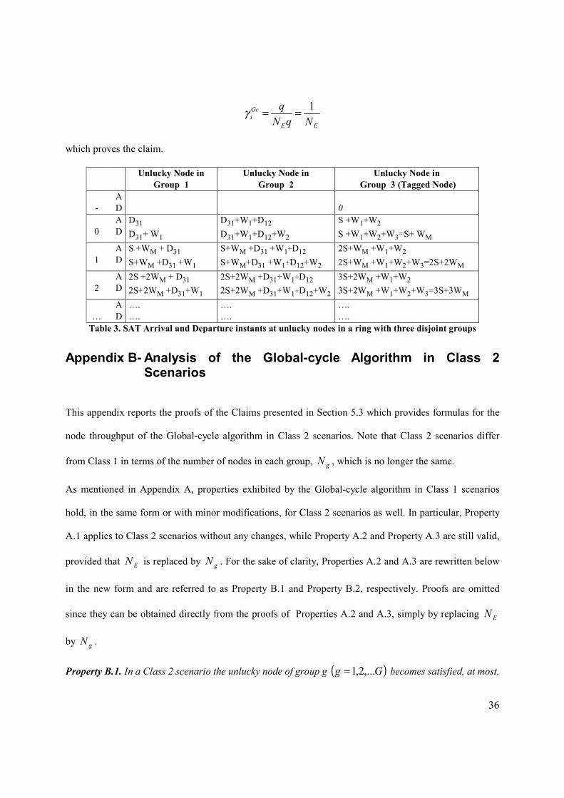
36

EE

Gci NqN

q 1==γ

which proves the claim.

Unlucky Node in Group 1

Unlucky Node in Group 2

Unlucky Node in Group 3 (Tagged Node)

-

A D

0

0

A D

D31 D31+ W1

D31+W1+D12 D31+W1+D12+W2

S +W1+W2 S +W1+W2+W3=S+ WM

1

A D

S +WM + D31 S+WM +D31 +W1

S+WM +D31 +W1+D12 S+WM+D31 +W1+D12+W2

2S+WM +W1+W2 2S+WM +W1+W2+W3=2S+2WM

2

A D

2S +2WM + D31 2S+2WM +D31+W1

2S+2WM +D31+W1+D12 2S+2WM +D31+W1+D12+W2

3S+2WM +W1+W2 3S+2WM +W1+W2+W3=3S+3WM

…

A D

…. ….

…. ….

…. ….

Table 3. SAT Arrival and Departure instants at unlucky nodes in a ring with three disjoint groups

Appendix B- Analysis of the Global-cycle Algorithm in Class 2 Scenarios

This appendix reports the proofs of the Claims presented in Section 5.3 which provides formulas for the

node throughput of the Global-cycle algorithm in Class 2 scenarios. Note that Class 2 scenarios differ

from Class 1 in terms of the number of nodes in each group, gN , which is no longer the same.

As mentioned in Appendix A, properties exhibited by the Global-cycle algorithm in Class 1 scenarios

hold, in the same form or with minor modifications, for Class 2 scenarios as well. In particular, Property

A.1 applies to Class 2 scenarios without any changes, while Property A.2 and Property A.3 are still valid,

provided that EN is replaced by gN . For the sake of clarity, Properties A.2 and A.3 are rewritten below

in the new form and are referred to as Property B.1 and Property B.2, respectively. Proofs are omitted

since they can be obtained directly from the proofs of Properties A.2 and A.3, simply by replacing EN

by gN .

Property B.1. In a Class 2 scenario the unlucky node of group g ( )Gg ,...2,1= becomes satisfied, at most,

37

qN g slots after the previous SAT release by the unlucky node itself.

Property B.2. In a Class 2 scenario if the shortest path criterion is used for packet routing (i.e., to choose

one of the two possible rings) and if the distance d between nodes is constant then dNS g 2≤ for

Ggg ,...2,1: =∀ .

As mentioned in Section 5.3 there are two different formulas for the node throughput, which are to be

used when MNSq ≤ and when MNSq > , respectively. Remember that MN is the number of nodes

in the largest group, i.e., ( )ggM NmaxN = . Claim B.1 reported below provides the formula for the case

MNSq ≤ .

Claim B.1. In Class 2 scenarios for Quota values q such that MNSq ≤ the throughput provided by the

Global-cycle algorithm to node i ( gNi ,...,2,1= ) in group g ( Gg ,...,2,1= ) is given by SqGci =γ .

Proof. The proof is similar to the proof of Claim A.1. By definition ( )ggM NmaxN = and, hence,

MNSq ≤ implies SqN g ≤ for Gg ,...2,1= . Since the SRT value cannot be less than S slots, by

Property B.1, any unlucky node is certainly satisfied at the SAT arrival. Hence, by Property A.1, the SAT

is never withheld and the time between two consecutive SAT releases by any node is equal to S. Since

each node transmits q packets between two consecutive SAT releases the claim is proved.

Claim B.2, which provides the formula for the case MNSq > , completes the analysis of the Global-

cycle algorithm in Class 2 scenarios.

Claim B.2. In Class 2 scenarios for Quota values q such that MNSq > the throughput provided by the

Global-cycle algorithm node i ( gNi ,...,2,1= ) in group g ( Gg ,...,2,1= ) is equal to MGci N1=γ .

Proof. To prove the above claim an approach similar to the one used in the proof of Claim A.2 is

followed. In fact, it will be shown that the time interval between two consecutive SAT releases operated

by the same node is constant and equal to qN M . Let G now denote the group with the largest number

38

of nodes (i.e., MG NN = ) and the tagged node be the unlucky node in this group. Again, assume that the

initial instant of the observation be at time instant at which the SAT is released by the tagged node.

Let ( )rgW be the SAT stop time at unlucky node g ( )Gg ,...2,1= in SAT rotation r ( ...,2,1,0=r ).

Obviously, SAT stop times experienced in the first SAT rotation (i.e., ( )0gW for Gg ...,,2,1= ) cannot be

determined since stop times related to the previous rotation are unknown. However, it can be easily

verified that the following conditions must be satisfied

( ) ( )SqNmaxW −≤≤ 10

1 ,00 [B.1]

( ) ( ) 1,...3,20 0 −=−≤≤ GgSqN0,maxW gg [B.2]

( ) ( ) 1,...3,201

0 −=−≤≤=

GgSqN0,maxW g

g

jj [B.3]

( ) ( )−

=

−−=1

1

01G

jjMG WSqNW [B.4]

Conditions [B.1] and [B.2] follow from the fact that the SRT value cannot be less than S slots and that, by

Property B.1, unlucky node g becomes satisfied qN g slot times after the last SAT release. Conditions

[B.3] arise from the fact that the SRT value related to an unlucky node includes the SAT stop times at the

upstream nodes (in the SAT direction). Condition [B.4] is obtained by observing that a) the SAT reaches

the tagged node at time ( )−

=

+1

1

0G

ggWS ; b) by conditions [B.3] it is ( ) qNWS M

G

gg ≤+

−

=

1

1

0 ; c) by Property

B.1, the tagged node becomes satisfied at time qNqN MG = .

By Property B.1 the SAT is released by the tagged node at time qN M and, then, a new SAT rotation starts

again. In the second and subsequent rotations the SAT stop times and the SAT rotation times (related to

any node) can be determined as a function of the SAT stop times experienced in the first SAT rotation

(i.e., ( )0gW for Gg ,...2,1= ). Specifically, it can be verified that the general formula for ( )r

gSRT , i.e., the

39

SRT value observed by the unlucky node g in the SAT rotation r is1

( )

( )

( ) ( )( ) ( )

�

�

�

−−+

=−= −

=

+ otherwiseWWWqN

gifWqNSRT

rg

g

j

rj

rjM

rgM

rg 1

1

1

1 [B.5]

Furthermore, by Property B.1, unlucky node g ( )Gg ,...2,1= releases the SAT qN g slots after the

previous SAT release. Hence, starting from [B.5] it is possible to compute ( ) ( ) ( )112

11 ...,,, GWWW (as

functions of ( ) ( ) ( )002

01 ...,,, GWWW ). Then it is possible to compute ( ) ( ) ( )22

22

1 ...,,, GWWW and so on.

However, the computation of the SAT stop times at unlucky nodes is not necessary for our purposes. In

fact, by using Property B.1, and by taking into account [B.5], with reference to node 1 it is

( ) ( )( )01

11 ,0 gM WqNqNmaxW +−=

( ) ( )( )11

21 22,0 gM WqNqNmaxW +−=

….

( ) ( )( )111 ,0 −+−= r

gMr WqrNqrNmaxW

….

By looking in detail at the above sequence it is possible to draw the following conclusion. If

MNN =1 then ( ) ( )11

−= rg

r WW for any r. Otherwise, it is possible to find a value 1r such that ( ) 011 =rW

and, hence, from that point onward all terms of the sequence will be null (since MNN <1 ). In short, there

exists a value 1r such that ( ) ( )rr WW 11

1 =+ for any 1rr ≥ independently of the initial value ( )01W .

If we are operating in the range 1rr ≥ equation [B.5] for 2=g can be written as

( ) ( )rM

r WqNSRT 22 −=

1 ( )r

gSRT is defined as the time interval between the r-th SAT release and the (r+1)-th SAT arrival at node g .

40

Hence, by following the same approach used for 1=g it is possible to find a value 12 rr ≥ such that

( ) ( )rr WW 21

2 =+ for any 2rr ≥ . In the range 2rr ≥ equation [B.5] for 3=g becomes

( ) ( )rM

r WqNSRT 33 −=

and the above approach can be reused. And so on and so forth. In conclusion, it is possible to find a value

121 ... rrrr GG ≥≥≥≥ − such that it is

( ) ( )G

rg

rg rrrGgWW ≥∀==+ :;...,,2,11 [B.6]

independently of the initial SAT stop times ( ) ( ) ( )002

01 ...,,, GWWW .

As for Class 1 scenarios, equalities in [B.6] imply that in steady state conditions (i.e., Grrr ≥∀ : ) the

time interval between two consecutive SAT releases operated by the same unlucky node is constant and

equal to qN M slots. By Property A.1 this conclusion can be extended to nodes which are not unlucky

nodes (at these nodes SAT release occurs immediately after reception). Since each node transmits q

packets in the time interval between two consecutive SAT releases the claim is proved.

Documents

Tradeoff between the Cycle Complexity and the Fairness of Ring