Tradeoffs in Neural Variational Inference · important characteristics of the observation, thus enabling data-efficient learning for recog-nition, classification, and causal modeling

Tradeoffs in Neural VariationalInference

Thesis

Ashwin D. D’Cruz

Supervisor: Dr. Sebastian NowozinProf. Bill Byrne

Department of EngineeringUniversity of Cambridge

This project proposal is submitted for the degree ofMaster Of Philosophy

Hughes Hall August 2017

Declaration

I, Ashwin D. D’Cruz, of Hughes Hall, being a candidate for the MPhil in Machine Learning,Speech and Language Technology, hereby declare that this report and the work described init are my own work, unaided except as may be specified below, and that the report does notcontain material that has already been used to any substantial extent for a comparable purpose.

Total word count: 13 732

Ashwin D. D’CruzAugust 2017

Acknowledgements

I would like to thank Dr. Sebastian Nowozin from Microsoft Research Cambridge forproposing this project, helping me get started with Chainer, and constantly providing usefulfeedback throughout the course of this project.

I’m also thankful to Prof. Bill Byrne for his guidance and advice during this time.

A special mention goes out to the MLSALT cohort. This year would have been nowhere nearas enjoyable without you. Thank you for your patience in explaining relatively easy conceptsto this simple engineer, always being down to go bug hunting, and celebrating our victorieswith a pint or three.

I would like to thank my parents, Gerard and Adeline D’Cruz, whose support remainedundiminished even over the distance. A shout out to my siblings, Nisha and Rushil; ourholiday together definitely refreshed me for the final sprint. I’ll never forget our walk from theforest. Last but not least, thank you Antrim for proof-reading my work and being interestedenough in it, to the point of reading more machine learning books than I.

Abstract

Humans understand the world on an operational and causal level, allowing us to make accu-rate predictions about the consequences of our actions, and enabling us to plan. What wouldit take to endow artificial intelligence with similar capabilities? An important component isthe ability to learn from observations, that is, to translate data into a model that has a higherlevel representation. Such representation abstracts away irrelevant variation but preservesimportant characteristics of the observation, thus enabling data-efficient learning for recog-nition, classification, and causal modeling. In machine learning, the field of unsupervisedlearning addresses the challenge of learning models from observations.

One recent advancement in this field has been the development of Variational Auto-Encoders(VAE) ([31], [54]). Since its inception, there have been several suggested improvements.While these works compare their results to the original VAE work, a thorough comparisonbetween these improvements is lacking.

In this work, we present a thorough comparison between several selected improvements. Wecompare the variational log likelihood between these models on three datasets of varyingcomplexity: MSRC-12 ([19]), MNIST ([37]), and celebA ([39]).

While variational lower bounds are often presented, most work often neglects to discussmodel complexity and the associated training times and convergence rates. We compare themodeling times for these various approaches to provide practical guidelines regarding thetrade-offs between the variational lower bound achieved and the run time required for training.

Finally, we contribute an extensive code repository implementing these state of the art ma-chine learning techniques on the datasets mentioned. These are developed using the Chainer([66]) framework. These implemented models are also available for use on other datasets.

Table of contents

List of figures xiii

List of tables xv

Nomenclature xix

1 Introduction 11.1 Motivation . . . . . . . . . . . . . . . . . . . . . . . . . . . . . . . . . . . 1

1.1.1 Unsupervised Learning . . . . . . . . . . . . . . . . . . . . . . . . 11.1.2 Variational Auto-Encoder . . . . . . . . . . . . . . . . . . . . . . 11.1.3 Research Aims and Scope . . . . . . . . . . . . . . . . . . . . . . 21.1.4 Organization . . . . . . . . . . . . . . . . . . . . . . . . . . . . . 3

2 Background 52.1 Deep Neural Networks . . . . . . . . . . . . . . . . . . . . . . . . . . . . 5

2.1.1 Notation . . . . . . . . . . . . . . . . . . . . . . . . . . . . . . . 62.1.2 History . . . . . . . . . . . . . . . . . . . . . . . . . . . . . . . . 82.1.3 Improvements . . . . . . . . . . . . . . . . . . . . . . . . . . . . . 9

2.2 Variational Inference . . . . . . . . . . . . . . . . . . . . . . . . . . . . . 112.3 Variational Auto-Encoder . . . . . . . . . . . . . . . . . . . . . . . . . . . 12

3 Improvements and Related Work 133.1 Importance Weighted Auto-Encoder . . . . . . . . . . . . . . . . . . . . . 133.2 Auxiliary Deep Generative Model . . . . . . . . . . . . . . . . . . . . . . 143.3 Skip Deep Generative Model . . . . . . . . . . . . . . . . . . . . . . . . . 153.4 Inverse Autoregressive Flow . . . . . . . . . . . . . . . . . . . . . . . . . 153.5 Householder Flow . . . . . . . . . . . . . . . . . . . . . . . . . . . . . . . 16

x Table of contents

4 Datasets and Experimental Procedure 194.1 MSRC-12 . . . . . . . . . . . . . . . . . . . . . . . . . . . . . . . . . . . 194.2 MNIST . . . . . . . . . . . . . . . . . . . . . . . . . . . . . . . . . . . . 214.3 celebA . . . . . . . . . . . . . . . . . . . . . . . . . . . . . . . . . . . . . 224.4 Methodology . . . . . . . . . . . . . . . . . . . . . . . . . . . . . . . . . 25

4.4.1 Warm Up . . . . . . . . . . . . . . . . . . . . . . . . . . . . . . . 254.4.2 Learning rate . . . . . . . . . . . . . . . . . . . . . . . . . . . . . 264.4.3 Evaluation . . . . . . . . . . . . . . . . . . . . . . . . . . . . . . 27

5 Results 295.1 Pose Likelihood . . . . . . . . . . . . . . . . . . . . . . . . . . . . . . . . 29

5.1.1 Architecture . . . . . . . . . . . . . . . . . . . . . . . . . . . . . . 295.1.2 Results . . . . . . . . . . . . . . . . . . . . . . . . . . . . . . . . 305.1.3 Discussion . . . . . . . . . . . . . . . . . . . . . . . . . . . . . . 32

5.2 MNIST Likelihood . . . . . . . . . . . . . . . . . . . . . . . . . . . . . . 395.2.1 Architecture . . . . . . . . . . . . . . . . . . . . . . . . . . . . . . 395.2.2 Results . . . . . . . . . . . . . . . . . . . . . . . . . . . . . . . . 405.2.3 Discussion . . . . . . . . . . . . . . . . . . . . . . . . . . . . . . 42

5.3 celebA Likelihood . . . . . . . . . . . . . . . . . . . . . . . . . . . . . . 465.3.1 Architecture . . . . . . . . . . . . . . . . . . . . . . . . . . . . . . 465.3.2 Results . . . . . . . . . . . . . . . . . . . . . . . . . . . . . . . . 475.3.3 Discussion . . . . . . . . . . . . . . . . . . . . . . . . . . . . . . 49

5.4 Pose Timing . . . . . . . . . . . . . . . . . . . . . . . . . . . . . . . . . . 545.4.1 Results . . . . . . . . . . . . . . . . . . . . . . . . . . . . . . . . 545.4.2 Discussion . . . . . . . . . . . . . . . . . . . . . . . . . . . . . . 55

5.5 MNIST Timing . . . . . . . . . . . . . . . . . . . . . . . . . . . . . . . . 595.5.1 Results . . . . . . . . . . . . . . . . . . . . . . . . . . . . . . . . 595.5.2 Discussion . . . . . . . . . . . . . . . . . . . . . . . . . . . . . . 60

5.6 celebA Timing . . . . . . . . . . . . . . . . . . . . . . . . . . . . . . . . 615.6.1 Results . . . . . . . . . . . . . . . . . . . . . . . . . . . . . . . . 615.6.2 Discussion . . . . . . . . . . . . . . . . . . . . . . . . . . . . . . 62

5.7 Practical Recommendations . . . . . . . . . . . . . . . . . . . . . . . . . . 62

6 Summary and Future Work 656.1 Summary . . . . . . . . . . . . . . . . . . . . . . . . . . . . . . . . . . . 656.2 Future Work and Extensions . . . . . . . . . . . . . . . . . . . . . . . . . 65

6.2.1 Inverse Autoregressive Flow on other datasets . . . . . . . . . . . . 65

Table of contents xi

6.2.2 Planar Flow model . . . . . . . . . . . . . . . . . . . . . . . . . . 666.2.3 Timing of celebA dataset . . . . . . . . . . . . . . . . . . . . . . . 666.2.4 Fine-tuning models . . . . . . . . . . . . . . . . . . . . . . . . . . 666.2.5 Convolutional layers . . . . . . . . . . . . . . . . . . . . . . . . . 676.2.6 Depth in stochastic layers . . . . . . . . . . . . . . . . . . . . . . 67

References 69

List of figures

1.1 VAE model. . . . . . . . . . . . . . . . . . . . . . . . . . . . . . . . . . . 2

2.1 Example of a deep neural network. . . . . . . . . . . . . . . . . . . . . . . 72.2 Closer look at an individual neuron. Image taken from [21]. . . . . . . . . . 72.3 Example of an auto-encoder. Image taken from [12]. . . . . . . . . . . . . 92.4 VAE model. . . . . . . . . . . . . . . . . . . . . . . . . . . . . . . . . . . 12

3.1 ADGM graphical model. The model on the left is the generative networkand the one of the right is the inference network. Image taken from [40]. . . 14

4.1 Pose data: Samples from the training dataset. Original datapoints are pro-vided as a 60 dimensional vector. This was reshaped to give 20 joints, eachas coordinate with 3 dimensions. . . . . . . . . . . . . . . . . . . . . . . . 20

4.2 MNIST data: Samples from the training dataset. Images contain 28x28,grayscale pixels. . . . . . . . . . . . . . . . . . . . . . . . . . . . . . . . . 21

4.3 celebA data: Samples from the training dataset. Images contain 218x178pixels with three channels: red, green, and blue. . . . . . . . . . . . . . . . 23

4.4 celebA data: Samples from the training dataset after we apply further crop-ping and scaling. Images contain 64x64 pixels with three channels: red,green, and blue. . . . . . . . . . . . . . . . . . . . . . . . . . . . . . . . . 24

5.1 Pose data: A single sample from the testing dataset and its various recon-structions with different models. All models only use a single Monte Carlosample for expectations. . . . . . . . . . . . . . . . . . . . . . . . . . . . 39

5.2 MNIST data: A single sample from the testing dataset and its various recon-structions with different models. All models only use a single Monte Carlosample for expectations. . . . . . . . . . . . . . . . . . . . . . . . . . . . 45

xiv List of figures

5.3 celebA data: ELBO on the validation set for various network architectures.The legend is (number of hidden units per layer, number of dimensions inthe latent space, number of hidden layer in the encoder and decoder). 1000training epochs were run but the validation ELBO was only recorded every 5epochs which is why the x-axis has a much smaller range. Additionally, weomit the results from the first 50 training epochs as these values were verysmall and prevented us from properly viewing the trends during later epochs. 47

5.4 celebA data: Reconstruction of a single sample from the tests dataset underseveral models. All models only use a single Monte Carlo sample forexpectations. . . . . . . . . . . . . . . . . . . . . . . . . . . . . . . . . . 52

5.5 celebA data: Sampling from models. All models only use a single MonteCarlo sample for expectations. . . . . . . . . . . . . . . . . . . . . . . . . 53

List of tables

5.1 Pose data: Network architecture. . . . . . . . . . . . . . . . . . . . . . . . 295.2 Pose data: average ELBO over the validation set (175,638 samples). We

also report the standard error of the mean (SEM). Models examined are thestandard VAE and IWAE. . . . . . . . . . . . . . . . . . . . . . . . . . . . 30

5.3 Pose data: average ELBO over the test set (175,638 samples). We also reportthe standard error of the mean (SEM). Models examined are the standardVAE and IWAE. . . . . . . . . . . . . . . . . . . . . . . . . . . . . . . . . 30

5.4 Pose data: average ELBO over the validation set (175,638 samples). Wealso report the standard error of the mean (SEM). Models examined are theADGM and SDGM. . . . . . . . . . . . . . . . . . . . . . . . . . . . . . . 31

5.5 Pose data: average ELBO over the test set (175,638 samples). We also reportthe standard error of the mean (SEM). Models examined are the ADGM andSDGM. . . . . . . . . . . . . . . . . . . . . . . . . . . . . . . . . . . . . 31

5.6 Pose data: average ELBO over the validation set (175,638 samples). Wealso report the standard error of the mean (SEM). Model examined is theHouseholder flow model. A single Monte Carlo sample was used for theexpectation. . . . . . . . . . . . . . . . . . . . . . . . . . . . . . . . . . . 31

5.7 Pose data: average ELBO over the test set (175,638 samples). We also reportthe standard error of the mean (SEM). Model examined is the Householderflow model. A single Monte Carlo sample was used for the expectation. . . 31

5.8 Pose data: average ELBO over the validation set (175,638 samples). We alsoreport the standard error of the mean (SEM). Model examined is the IAFmodel. A single Monte Carlo sample was used for the expectation. . . . . . 32

5.9 Pose data: average ELBO over the test set (175,638 samples). We also reportthe standard error of the mean (SEM). Model examined is the IAF model. Asingle MC sample was used for the expectation. . . . . . . . . . . . . . . . 32

xvi List of tables

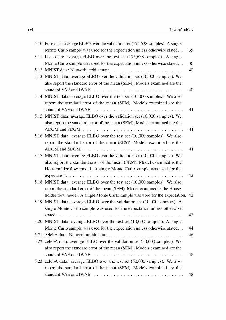
5.10 Pose data: average ELBO over the validation set (175,638 samples). A singleMonte Carlo sample was used for the expectation unless otherwise stated. . 35

5.11 Pose data: average ELBO over the test set (175,638 samples). A singleMonte Carlo sample was used for the expectation unless otherwise stated. . 36

5.12 MNIST data: Network architecture. . . . . . . . . . . . . . . . . . . . . . 405.13 MNIST data: average ELBO over the validation set (10,000 samples). We


5.14 MNIST data: average ELBO over the test set (10,000 samples). We alsoreport the standard error of the mean (SEM). Models examined are thestandard VAE and IWAE. . . . . . . . . . . . . . . . . . . . . . . . . . . . 41

5.15 MNIST data: average ELBO over the validation set (10,000 samples). Wealso report the standard error of the mean (SEM). Models examined are theADGM and SDGM. . . . . . . . . . . . . . . . . . . . . . . . . . . . . . . 41

5.16 MNIST data: average ELBO over the test set (10,000 samples). We alsoreport the standard error of the mean (SEM). Models examined are theADGM and SDGM. . . . . . . . . . . . . . . . . . . . . . . . . . . . . . . 41

5.17 MNIST data: average ELBO over the validation set (10,000 samples). Wealso report the standard error of the mean (SEM). Model examined is theHouseholder flow model. A single Monte Carlo sample was used for theexpectation. . . . . . . . . . . . . . . . . . . . . . . . . . . . . . . . . . . 42

5.18 MNIST data: average ELBO over the test set (10,000 samples). We alsoreport the standard error of the mean (SEM). Model examined is the House-holder flow model. A single Monte Carlo sample was used for the expectation. 42

5.19 MNIST data: average ELBO over the validation set (10,000 samples). Asingle Monte Carlo sample was used for the expectation unless otherwisestated. . . . . . . . . . . . . . . . . . . . . . . . . . . . . . . . . . . . . . 43

5.20 MNIST data: average ELBO over the test set (10,000 samples). A singleMonte Carlo sample was used for the expectation unless otherwise stated. . 44

5.21 celebA data: Network architecture. . . . . . . . . . . . . . . . . . . . . . . 465.22 celebA data: average ELBO over the validation set (50,000 samples). We


5.23 celebA data: average ELBO over the test set (50,000 samples). We alsoreport the standard error of the mean (SEM). Models examined are thestandard VAE and IWAE. . . . . . . . . . . . . . . . . . . . . . . . . . . . 48

List of tables xvii

5.24 celebA data: average ELBO over the validation set (10,000 samples). Wealso report the standard error of the mean (SEM). Models examined are theADGM and SDGM. . . . . . . . . . . . . . . . . . . . . . . . . . . . . . . 48

5.25 celebA data: average ELBO over the test set (50,000 samples). We alsoreport the standard error of the mean (SEM). Models examined are theADGM and SDGM. . . . . . . . . . . . . . . . . . . . . . . . . . . . . . . 49

5.26 celebA data: average ELBO over the validation set (50,000 samples). Wealso report the standard error of the mean (SEM). Model examined is theHouseholder flow model. A single Monte Carlo sample was used for theexpectation. . . . . . . . . . . . . . . . . . . . . . . . . . . . . . . . . . . 49

5.27 celebA data: average ELBO over the test set (50,000 samples). We also reportthe standard error of the mean (SEM). Model examined is the Householderflow model. A single Monte Carlo sample was used for the expectation. . . 49

5.28 celebA data: average ELBO over the validation set (50,000 samples). Asingle Monte Carlo sample was used for the expectation unless otherwisestated. . . . . . . . . . . . . . . . . . . . . . . . . . . . . . . . . . . . . . 50

5.29 celebA data: average ELBO over the test set (50,000 samples). A singleMonte Carlo sample was used for the expectation unless otherwise stated. . 50

5.30 Pose data: average times over the training and validation set (351,275 and175,638 samples respectively). We also report the standard deviation inbrackets. Model examined is the VAE. . . . . . . . . . . . . . . . . . . . . 54

5.31 Pose data: average times over the training and validation set (351,275 and175,638 samples respectively). We also report the standard deviation inbrackets. Model examined is the IWAE. . . . . . . . . . . . . . . . . . . . 54

5.32 Pose data: average times over the training and validation set (351,275 and175,638 samples respectively). We also report the standard deviation inbrackets. Models examined are the ADGM and SDGM. A single MonteCarlo sample was used for the expectation. . . . . . . . . . . . . . . . . . . 55

5.33 Pose data: average times over the training and validation set (351,275 and175,638 samples respectively). We also report the standard deviation inbrackets. Model examined is the Householder flow. A single Monte Carlosample was used for the expectation. . . . . . . . . . . . . . . . . . . . . . 55

5.34 Pose data: average times over the training and validation set (351,275 and175,638 samples respectively). We also report the standard deviation inbrackets. Model examined is the IAF. A single Monte Carlo sample wasused for the expectation. . . . . . . . . . . . . . . . . . . . . . . . . . . . 55

xviii List of tables

5.35 MNIST data: average times over the training and validation set (50,000and 10,000 samples respectively). We also report the standard deviation inbrackets. Model examined is the VAE. . . . . . . . . . . . . . . . . . . . . 59

5.36 MNIST data: average times over the training and validation set (50,000and 10,000 samples respectively). We also report the standard deviation inbrackets. Model examined is the IWAE. . . . . . . . . . . . . . . . . . . . 59

5.37 MNIST data: average times over the training and validation set (50,000and 10,000 samples respectively). We also report the standard deviation inbrackets. Models examined are the ADGM and SDGM. A single MonteCarlo sample was used for the expectation. . . . . . . . . . . . . . . . . . . 59

5.38 MNIST data: average times over the training and validation set (50,000and 10,000 samples respectively). We also report the standard deviation inbrackets. Model examined is the Householder flow. A single Monte Carlosample was used for the expectation. . . . . . . . . . . . . . . . . . . . . . 59

5.39 celebA data: average times over the training and validation set (100,000and 50,000 samples respectively). We also report the standard deviation inbrackets. Model examined is the VAE. . . . . . . . . . . . . . . . . . . . . 61

5.40 celebA data: average times over the training and validation set (100,000and 50,000 samples respectively). We also report the standard deviation inbrackets. Model examined is the IWAE. . . . . . . . . . . . . . . . . . . . 61

5.41 celebA data: average times over the training and validation set (100,000and 50,000 samples respectively). We also report the standard deviation inbrackets. Models examined are the ADGM and SDGM. A single MonteCarlo sample was used for the expectation. . . . . . . . . . . . . . . . . . . 61

5.42 celebA data: average times over the training and validation set (100,000and 50,000 samples respectively). We also report the standard deviation inbrackets. Model examined is the Householder flow. A single Monte Carlosample was used for the expectation. . . . . . . . . . . . . . . . . . . . . . 61

Nomenclature

Acronyms / Abbreviations

ADGM Auxiliary Deep Generative Model

AE Auto-Encoder

BP Back-propagation

DNN Deep Neural Network

ELBO Evidence Lower Bound

GPU Graphics Processing Unit

IAF Inverse Autoregressive Flow

IWAE Importance Weighted Auto-Encoder

KL Kullback-Leibler

MC Monte Carlo

NN Neural Network

ReLU Rectified Linear Unit

SDGM Skip Deep Generative Model

SGD Stochastic Gradient Descent

SGVB Stochastic Gradient Variational Bayes

VAE Variational Auto-Encoder

VI Variational Inference

Chapter 1

Introduction

1.1 Motivation

1.1.1 Unsupervised Learning

Unsupervised learning is a field of machine learning in which the machine attempts todiscover structure and patterns in a dataset ([24]). In the case where the machine has toestimate the probability of a new data point xn given some previous points x1, ...,xn−1, wecan develop a model that is useful for outlier detection. Unsupervised learning is also usefulwithin the context of representation learning : given some data, identify the underlying latentfactors that explain the observations.

Representation learning is useful for many applications ([4]). Learned good representa-tions can be used as inputs for supervised machine learning systems ([57]) such as speechrecognition ([59]), object recognition ([34]), and natural language processing ([2]).

1.1.2 Variational Auto-Encoder

The applications outlined above provide a strong basis for research into representation learn-ing. Recently, one approach to this has been the Variational Auto-Encoder (VAE) ([31], [54]).This is an efficient probabilistic deep learning method that has gained a lot of popularityrecently. It is widely applied due to its ease of use and promising results ([17]).

The basic VAE model is shown in Figure 1.1. The generative network is moving from thelatent distribution z to distribution x and is parametrized by θ as shown by the solid lines. Totrain the generative network, a second network called the inference network is built and this

2 Introduction

network is shown by the dashed line. Here we move from the distribution of data to the latentspace with a network parametrized by φ . The two are optimized together using stochasticgradient descent (SGD). The quality of inference and the generative process are dependenton the accuracy of the inference network.

There have been several proposals on how to improve the inference network of the VAEwhich would improve the model’s capabilities. While these improvements draw comparisonsto the original VAE work, a thorough comparison between the different improvements islacking in the community. This is the gap we seek to close with this work.

Fig. 1.1 VAE model.

1.1.3 Research Aims and Scope

Our work is concerned with a thorough quantitative evaluation of five modifications of theoriginal VAE model on three datasets.We compare the following works:

• Importance Weighted Auto-Encoder (IWAE) ([10])

• Auxiliary Deep Generative Model (ADGM) ([40])

• Skip Deep Generative Model (SDGM) ([40])

• Householder Flow Model ([67])

• Inverse Autoregressive Flow (IAF) Model ([33])

More information on these is provided in Chapter 3.

The following datasets are modeled:

• MSRC-12 ([19])

1.1 Motivation 3

• MNIST ([37])

• celebA ([39])

More information on these is provided in Chapter 4.

The common metric used in comparing deep generative models is the variational lower bound;this metric is explained in Section 2.2 . We will also report the same metric. Additionally,we will investigate the modeling time taken by these various approaches. We will considerdifferent aspects of this time metric. Of concern to us is how long the encoding and decodingprocess take as well as the update procedure for the parameters of the networks.

1.1.4 Organization

The remaining chapters are organized as follows:Chapter 2 provides some background information on deep neural networks (DNNs) andvariational inference (VI): two key building blocks in the development of VAEs. A reviewof VAE improvements and related work is presented in Chapter 3. The datasets used andmethodology are detailed in Chapter 4. Chapter 5 discusses the results of our work andChapter 6 proposes avenues for future work.

Chapter 2

Background

In this chapter, we will provide some background on the theory that forms the foundation forthe rest of our work. In particular, we will cover the basics of deep neural networks (DNNs),including details about the training procedure and methods to augment this. We will alsopresent a brief overview of variational inference (VI). Finally, we will show how these twoconcepts, DNNS and VI, meet in the form of Variational Auto-Encoders (VAEs).

For a more complete overview of DNNS, the reader is encouraged to look at the work of[58]. Similarly, please refer to [8] for a thorough review of VI.

2.1 Deep Neural Networks

For a long time, many machine learning techniques and algorithms required careful featureengineering from domain experts. Raw input would be processed through carefully con-structed steps to obtain features that were thought to be useful for the task at hand. Examplesof this include Mel-frequency cepstral coefficients for speech related tasks ([6, 22]) or SIFTfeatures for computer vision ([5, 69]).

Within machine learning, representation learning allows a machine to automatically extractuseful features from the raw input that can be used to solve specific tasks ([4]). Deep-learningmethods are a form of representation learning. Specifically, neural networks (NNs) transformdata from one representation into a more abstract one. DNNs do this repeatedly, learn-ing a hierarchy of representations. Simple non-linear modules are used to transform onerepresentation of the data into a higher, increasingly abstract representations ([38]). Thisbegins with the raw input such as raw pixels of an image or raw waveforms and consecutivetransformations could lead to features such as the class of the object within a image or the

6 Background

identity of a speaker. Given enough transformations, arbitrarily complex functions of the rawinput can be learned.

The key aspect here is that the DNN is capable of automatically learning good represen-tations by adjusting its parameters through the process of back-propagation. As this is ageneral training procedure, deep neural networks can be easily applied to a host of tasks withminimum domain expertise and manual feature crafting.

2.1.1 Notation

Figure 2.1 shows a DNN. This network has 4 input features, 4 output features and 2 hiddenlayers (each with 5 nodes). We adopt the similar notation to [21] and briefly outline it here.

A set of x(k) form the inputs to layer k. x(1) are the initial features from the dataset we areworking with. At each layer, we denote the output as y(k). Note that since the output fromlayer k are inputs to layer (k+1), y(k) can also be referred to as x(k+1).

Figure 2.2 displays a more localized view of a single node. wi refers to the weights at agiven node and φ refers to the non-linearity applied to the output of the weights and inputs.There are various non-linearities that can be used and the choices we considered are given inSection 2.1.3.

At each layer, the following equation applies:

yki = φ(w

′ix

(k)+bi) = φ(z(k)i ) (2.1)

Also of note is the number of parameters within particular DNN architectures. For a DNNsuch as that shown in Figure 2.1, the number of parameters can be calculated the followingequation:

N = d ×N(1)+K ×N(L)+L−1

∑k=1

N(k)×N(k+1) (2.2)

Where:

• L is the number of hidden layers

• N(k) is the number of nodes for layer k

2.1 Deep Neural Networks 7

• d is the input vector size, K is the output size

As seen, the number of parameters depends on both the width (number of nodes per layer)and depth of the network. [3, 35] showed that increasing the depth of a network is morefavourable than increasing the width with regards to obtaining a more powerful networkwhile minimizing the number of parameters used. More recent work by [68] has shown thatthis doesn’t neccessarilly hold true for all types of network architectures. In our work, wewill examine the differing widths and depths required to model the different datasets.

x1

x2

x3

x4

y1

y2

y3

y4

Hiddenlayer

Inputlayer

Hiddenlayer

Outputlayer

Fig. 2.1 Example of a deep neural network.

Fig. 2.2 Closer look at an individual neuron. Image taken from [21].

8 Background

2.1.2 History

The idea of representing logical connections with structures mimicking biological neurons isnot a new one. Early work in the 1940s such as [42] represented calculus operations withneural network architectures but these networks did not have the ability to learn. Followingthis, neural networks with simple training procedures were developed ([46], [55]) althoughthese network architectures lacked depth.

Work by [26] examined the visual cortex of a cat and found that different cells pickedup different features. Specifically, they categorized the cells into two general categories:simple and complex. The complex cells were more robust to spatial invariance. The workof [26] was significant in inspiring the Neocognitron ([20]), the first deep neural network.The hierarchy proposed by [20] was similar to the visual nervous system proposed by[26]. Additionally, [20] introduced the concept of convolutional neural networks (convnets)which allowed them to achieve spatial invariance, similar to the complex cells posited by [26].In the present day, convnets are used in state of the art machine learning systems ([34, 48, 52])

In general, the weights of any arbitrary function can be updated through steepest descent inthe weight space ([9]) using iterative applications of the chain rule. The process of propagat-ing the error from the cost function from the final layer through the previous layers is knownas back-propagation (BP). The work of [56] went a long way in popularizing the use of BPfor the use of DNNs. BP is still the most widely used method for training DNNs. For moredetails on BP, please see [47, 56].

Following on, several improvements to optimization procedure have been suggested. Wediscuss the relevant improvements to our work in Section 2.1.3.

It is also important to mention the type of DNN developed by [56]: the Auto-Encoder(AE). In this DNN, an input vector is mapped to a lower dimensional representation (theencoding process) and then this new representation is used to reconstruct the original input(the decoding process). An example of what this network might look like is shown in Figure2.3.

2.1 Deep Neural Networks 9

Fig. 2.3 Example of an auto-encoder. Image taken from [12].

This was important from a representation learning point of view but is of particular interestto our work as VAEs have a strong parallel to AEs.

While the work of [56] was vital in reviving research interest in DNNs, it was the achievementof DNNs in various competitions and industrial applications that would continue to drivedevelopment in this field. For example, MNIST records were set using DNNs by [61], [51],[14], and [13] in 2003, 2006, 2010, and 2012 respectively.

2.1.3 Improvements

Optimization

Adagrad ([18]) is a modification to the stochastic gradient descent (SGD) optimization pro-cedure to produce an adaptive learning rate method. Under the standard SGD procedure, thesame learning rate is used to update all parameters. With Adagrad however, each parameterobtains a specialised learning rate. Specifically, the more frequently a particular weight isupdated, the smaller the learning rate for that weight. Weights that are infrequently updatedare linked to sparse features. So in effect, Adagrad emphasizes learning from sparse features,believing them to be informative. The learning rate for all parameters tends towards 0 as afunction of iterations and one of the disadvantages of Adagrad is that this often happens too

10 Background

early, halting the learning procedure before the model has reached an optimal point.

An improvement on this is RMSProp ([65]). Where Adagrad uses an average of squaredgradients to control the decay rate, RMSProp uses a moving average of the squared gradientsinstead. By limiting the history considered, the decay isn’t as aggressive and the learningprocedure doesn’t stop as early.

Building on this work is Adam ([30]). The squared gradients decay component of RMSpropis also known as second order momentum. Adam utilizes this but also uses first ordermomentum: a moving average of the gradient. This has been shown to lead to convergencein fewer iterations ([30]). In our work, we have chosen to use the Adam optimizer.

Activation Functions

The rectified linear unit or ReLU ([45]) non-linear activation function is commonly used inDNNs. It behaves in the following manner:

f (z) = max(0,z) (2.3)

Compared to previous work such as the sigmoid or tanh activation functions, ReLu functionsdo not suffer from over-saturated activations. However, they can lead to ’dead’ neurons if theinput remains negative ([29]).

A recent proposal that overcomes this limitation is the concatenated relu or CReLU by [60].Here, the activation is given by:

f (z) = (max(0,x),max(0,−x)) (2.4)

This activation function is capable of utilizing both positive and negative Z (unlike thestandard ReLU which returns 0 for negative inputs) while still having the property of being anon-saturating non-linearity. We use CReLU in our implementations.

Batch Normalization

Batch normalization ([27]) is a recently proposed technique to assist training in DNNs. Itis common to normalize the input to a DNN to avoid any features having differing levelsof impacts due to their respective scales. However, after passing through layers of a DNN,

2.2 Variational Inference 11

transformations might have undone this affect and the distributions of data at different depthsof the network may be extremely disparate. [27] refer to this phenomenon as internalcovariate shift and note that it causes difficulties with:

• Choosing effective learning rates.

• Parameter initialization.

• Saturating non-linearities.

[27] proposed a solution: normalizing the input at each layer after the weighted sum butbefore the non-linearities. The introduction of normalization at each layer of the networkrather than only at the input level not only overcomes the difficulties mentioned earlier butwas also shown to lead to improved final models ([27]).

2.2 Variational Inference

VI casts statistical inference problems as optimization problems ([28]). Specifically, whenperforming Bayesian inference, it may be intractable to use the exact posterior p(z|x). Instead,an approximate posterior, qφ (z|x), is chosen and the values for the parameters, φ , of thisapproximation are optimized to maximize a lower bound on the marginal likelihood. The setof equations we are interested in are shown below:

logp(x)−DKL(qφ (z|x)||p(z|x)) = Eqφ[logp(x,z)− logqφ (z|x)] (2.5a)

logp(x)⩾ Eqφ[logp(x,z)− logqφ (z|x)] = L (2.5b)

Equation 2.5a relates the true log likelihood, logp(x) to the true and approximate posteriors.Equation 2.5b depicts the Evidence Lower Bound (ELBO), L, which is the quantity we opti-mize as it doesn’t involve the intractable posterior that was present in the Kullback–Leibler(KL) divergence term. Note that since the KL divergence is non-negative, the ELBO is alower bound on the exact log likelihood.

When performing variational inference, we choose the family of distributions whose parame-ters we optimize. It is common to use mean field variational inference whereby the variablesof the variational distribution are assumed to be independent. Due to this strong assumption,the variational family of distributions often does not contain the true posterior distribution([7]). This is important to note for two reasons:

12 Background

• While it is possible to find parameters φ such that qφ (z|x) matches p(z|x) exactly,we have stated that due to the strong assumption placed on the family of variationaldistributions, it is unlikely that the approximate posterior will match the true posterior.

• This weakness introduced by the family of variational distributions is what the sug-gested improvements we are examining seek to overcome.

2.3 Variational Auto-Encoder

VAEs combine DNNs and VI. Figure 2.4 depicts the construction of Equation 2.5b under theVAE framework. The approximate posterior, qφ (z|x), is modeled using a DNN ([31, 54]).We also have a generative model pθ (z,x) with parameters θ . The two are jointly optimizedusing VI techniques.

Fig. 2.4 VAE model.

One of the important contributions of [31, 54] was the development of the reparametrizationtrick and its subsequent use in the Stochastic Gradient Variational Bayes (SGVB) estimator.This practical gradient estimator does not suffer from high variance compared to previouswork such as [50].

Chapter 3

Improvements and Related Work

In this chapter, we examine the proposed improvements to the Variational Auto-Encoder(VAE) in more depth.

3.1 Importance Weighted Auto-Encoder

The Importance Weighted Auto-Encoder (IWAE) was developed by [10]. Unlike most ofthe improvements we will discuss, the IWAE uses the same architecture as the standardVAE. Instead, the IWAE better utilizes the modeling capacity of the network by using atighter log-likelihood lower bound or evidence lower bound (ELBO). This modified ELBOis derived from importance weighting and is shown in Equation 3.1a:

Lk(x) = Ez1,...,zk∼qφ (z|x)

[log

1k

k

∑i=1

pθ (x,zi)

qφ (zi|x)

](3.1a)

One of the variational assumptions is that the latent space is approximately factorial. Thestandard VAE objective heavily penalizes samples that don’t adhere to this assumption.However, as the true posterior is unlikely to be approximately factorial, the standard VAEobjective may be ignoring samples that are actually more likely under the true posterior.The IWAE relaxes this assumption of an approximately factorial posterior using importancesampling. It considers samples that don’t adhere to this assumption and uses importanceweighting to better take into account all samples from the approximate posterior, not just onesthat satisfy the variational assumption. This relaxation on the sampling procedure allows amore flexible generative network to be trained. [10] focused on showing how this modifiedELBO was strictly tighter than the standard VAE ELBO and showed how as more sampleswere used, the modified ELBO approached the true log likelihood. Recent work by [15]

14 Improvements and Related Work

expanded on the work by [10] to show how using the IWAE objective was equivalent to usingthe standard VAE objective but with a more complex approximate posterior distribution thatdid not strictly adhere to the standard variational assumptions.

3.2 Auxiliary Deep Generative Model

Auxiliary Deep Generative Models (ADGMs) were developed by [40]. In this work, theyfocused on the semi-supervised task where datapoints x had labels y. For this task, thegraphical model for the inference and generative networks of the ADGM are shown in Figure3.1.

Fig. 3.1 ADGM graphical model. The model on the left is the generative network and theone of the right is the inference network. Image taken from [40].

The main contribution here is the introduction of the set of auxiliary latent variables, a. Thisauxiliary variable helps tie together the other variables in the network without requiringthe latent space z to become significantly more complex. For the task we are interested in,unsupervised learning, the probabilistic model is similar to that shown in Figure 3.1 butwithout the inclusion of the labels y. In this task, we can see from the inference networkthat a acts as a feature extractor on x and that these additional features are used to develop abetter latent space z. Specifically, [40] note that with this model the latent dimensions of zcan be correlated through a. Note however that the generative procedure is still the same aswhat the standard VAE uses and the variable a is not necessary for sampling. It is only usefulfor the training procedure in developing better trained inference and generative networks.

3.3 Skip Deep Generative Model 15

3.3 Skip Deep Generative Model

Skip Deep Generative Models (SDGMs) were also developed by [40] are come about from achange to the ADGM. Specifically, in Figure 3.1, the arrow between a and x is reversed inthe generative network but the inference network remains the same. Essentially, this pulls ainto the generative process. In fact, what we now have is a 2 layer stochastic model wherea is the added depth in the latent space. However, unlike the deep latent models used by[32, 54], here z feeds directly into x in the generative model through a skip connection. [40]note that this skip connection was crucial in allowing end-to-end training unlike [32] whocould not achieve convergence with end-to-end training and had to resort to using layer wisetraining instead.

3.4 Inverse Autoregressive Flow

Inverse Autoregressive Flow (IAF) models were developed by [33]. At the core of theirmethod are Gaussian autoregressive functions which in the past have been used for densityestimation tasks ([23, 48, 49]). [33] show that such functions can be used for invertiblenon-linear transformations of the latent space, resulting in the IAF which is an example of aflow under the normalizing flow ([53, 63, 64]) framework.

Normalizing flows were first developed by [63, 64]. In these works, they proposed that aseries of invertible mappings can be applied to simple probability distributions to obtaina more complex one. [53] utilized this idea for the purpose of enriching the approximateposterior in VAEs. Specifically, we begin with the approximate factorized posterior z0 andafter T transformations, obtain a more flexible posterior, zT . The focus of [53] was on aspecific parametrized family of transformations called planar flows. This transformation wasgiven by Equation 3.2a:

ft(zt−1) = zt−1 +uh(wTzt−1 +b) (3.2a)

In Equation 3.2a, u and w are vectors, b is a scalar and h is a non-linearity. Given these,one interpretation of the planar flow transformation is a multi layer perceptron bottleneckwith a single unit ([33]). Due to this, this family of transformations is ill-suited to capturedependencies in a high dimensional latent space as a long series of transformations would berequired.

16 Improvements and Related Work

The IAF model proposed by [33] avoids this issue because their inverse autoregressivefunctions can be parallelized. This allows better scaling to high dimensional latent spacesas the absence of a bottleneck means that fewer transformations are required to capturethe dependencies between the dimensions. [33] note that given even a single IAF step, aGaussian posterior with a diagonal covariance matrix can be transformed into one with a fullcovariance matrix.

3.5 Householder Flow

The Householder flow model developed by [67] is another example of a normalizing flowmethod. Within this framework, [67] state that their Householder flow method is an exampleof a volume preserving flow in which the Jacobian-determinants involved with the transfor-mations equals 1. Hence the motivation for this method is that the Jacobian-determinantsdo not need to be explicitly calculated for each transformation, significantly reducing thecomputational complexity.

The core principle behind the Householder flow model is that full covariance matrices can bedecomposed in the following way:

Σ = UDU′

(3.3a)

Where U is an orthogonal matrix and D is a diagonal matrix. If the covariance matrix of z0

corresponds to D, then to achieve the full covariance matrix, all that is left is to model U.[67] suggest the following method to model U:

U = HTHT−1...H1 (3.4a)

Where T is less than or equal to the dimensionality of U and Ht are Householder matrices.

The Householder transformation and matrix are shown in Equations 3.5a and 3.5b:

zt =

(I−2

vtv′t

||vt||2

)zt−1 (3.5a)

= Htzt−1 (3.5b)

3.5 Householder Flow 17

The initial Householder vector v0 is an output from the encoder network. Subsequent vt

are obtained by inputting vt−1 into a linear layer. Applications of the Householder flowhelp transform a factorized latent space into one with an approximate full covariance matrix,which is believed to be a closer approximation to the true posterior. It is worth noting thatsince Householder transformations are linear, they are cheaper to compute compared tonon-linear transformations such as the IAF ([33]).

Chapter 4

Datasets and Experimental Procedure

We discuss the datasets used in this work, highlighting our motivation for using each one.Additionally, we also present our methodology.

4.1 MSRC-12

The MSRC-12 dataset ([19]) consists of sequences of human movements collected usingthe Kinect system. In this work, for clarity, we often refer to this dataset as the Pose dataset.Each datapoint consists of 60 points which form subsets of 3 points corresponding to 20human joint locations. Each sequence is associated with 1 of 12 gestures. The dataset canbe obtained from [44]. For the purpose of our work, we consider the individual frames ofhuman movements with no regards for sequences or the gesture label. There are 702,551frames in total. We split the frames into the following subsets:

• 321,275 samples for the training set

• 175,368 samples for the validation set

• 175,368 samples for the testing set

Figure 4.1 shows a few examples of these frames.

20 Datasets and Experimental Procedure

(a) Sample 1 (b) Sample 2

(c) Sample 3 (d) Sample 4

Fig. 4.1 Pose data: Samples from the training dataset. Original datapoints are provided asa 60 dimensional vector. This was reshaped to give 20 joints, each as coordinate with 3dimensions.

We chose to investigate this dataset as there is a lot of structure within a single frame. Aspoints correspond to locations of humans joints, there is a strict order imposed on the loca-tion of joints relative to each other. The network would have to learn the general gestureswhile also learning this underlying structure and connectivity between the various joints.Furthermore, as this dataset is fairly new, we are interested in determining how well suitedVariational Auto-Encoders (VAEs) are for this task.

4.2 MNIST 21

4.2 MNIST

The MNIST dataset ([37]) has become a classic dataset in the machine learning community.It consists of 28x28, greyscale pixel images of handwritten digits, specifically the integers0 through 9. For our work, we disregard the labels provided with each image as we areinterested in an unsupervised learning task. There are 70,000 images in total which we splitas such:


• 10,000 samples for the validation set

• 10,000 samples for the testing set

Figure 4.2 shows a few examples of these images.



Fig. 4.2 MNIST data: Samples from the training dataset. Images contain 28x28, grayscalepixels.


4.3 celebA

The celebA dataset ([39]) consists of more than 200,000 images of celebrity faces. For ourwork, we consider 200,000 of these which we split as follows:




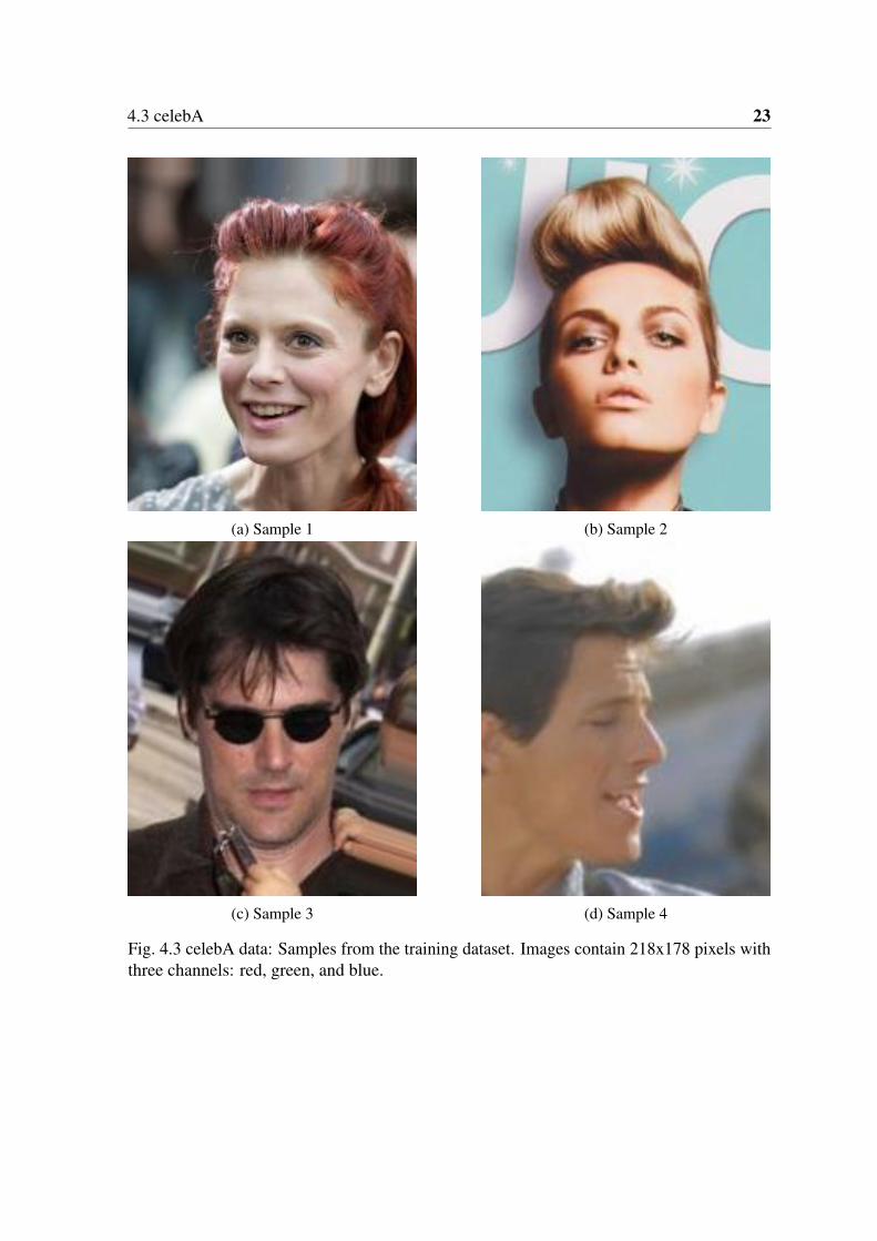
While each image comes with 40 different attributes, we ignore these as we are focused onan unsupervised learning task. [39] provides two versions of this dataset. One consists of theoriginal data they gathered while with the other, the original data is first roughly aligned usinga similarity transformation based on the eye locations before being scaled to be 218*178pixels. These images contain 3 channels: red, green, and blue. Figure 4.3 shows a few imagesfrom this second version of this dataset. We chose these four images to showcase here asthey highlight the variety present in the celebA dataset. Figure 4.3a shows a more ’casual’photo. In contrast, Figure 4.3b was taken in a more professional setting. Here, their face isdirectly facing the camera and while there is some detail in the background, it is not blurred.Figure 4.3c has a very distorted background that likely arose from the aligning and similaritytransformation applied by [39]. Figure 4.3d is an example of where the photo was not takenfront on.

4.3 celebA 23



Fig. 4.3 celebA data: Samples from the training dataset. Images contain 218x178 pixels withthree channels: red, green, and blue.




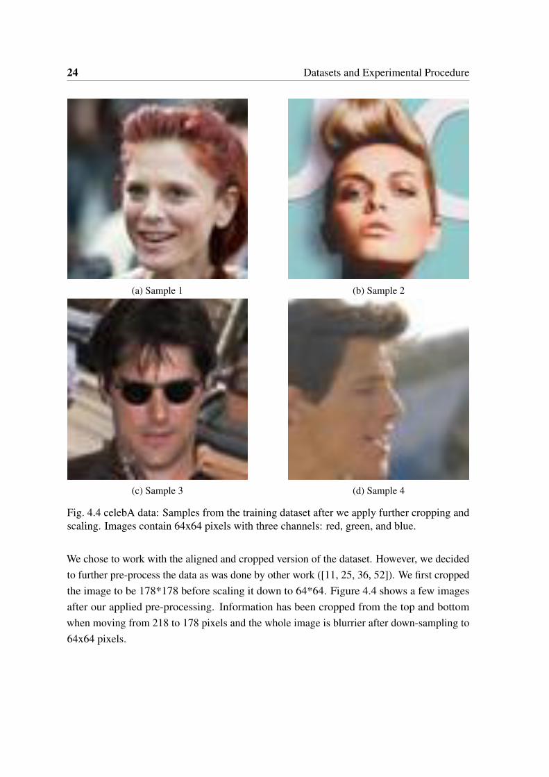
Fig. 4.4 celebA data: Samples from the training dataset after we apply further cropping andscaling. Images contain 64x64 pixels with three channels: red, green, and blue.

We chose to work with the aligned and cropped version of the dataset. However, we decidedto further pre-process the data as was done by other work ([11, 25, 36, 52]). We first croppedthe image to be 178*178 before scaling it down to 64*64. Figure 4.4 shows a few imagesafter our applied pre-processing. Information has been cropped from the top and bottomwhen moving from 218 to 178 pixels and the whole image is blurrier after down-sampling to64x64 pixels.

4.4 Methodology 25

We chose to examine this dataset as it was a fairly complex one. While it is also vision basedlike MNIST, the dimensionality here is larger and there are also 3 channels. Furthermore,these are facial images rather than hand-written digits and hence the underlying manifoldshould be more complex.

4.4 Methodology

We present the general methodology applied to each dataset while details of the networkarchitecture for each dataset are given in Chapter 5.

For each dataset, we first chose one or more architectures to investigate. In this initialinvestigation, we focused on the convergence rate on the validation set; specifically, if theevidence lower bound (ELBO) decreases (indicating overfitting) and how many epochs wererequired to reach convergence. These investigations were carried out using the plain VAEmodel. With regards to network architecture, here are the basic hyper-parameters we focusedon:

• Number of hidden units per hidden layer

• Dimensionality of the latent space

• Number of hidden layers in the encoder and decoder

• Batch size

In addition to this, we also focused on two additional settings: a warm up period for theKullback–Leibler (KL) divergence term and the learning rate for the optimizer. We brieflydescribe the motivations for these.

4.4.1 Warm Up

Equation 2.5b can also be rewritten as the following:

L =−KL(qφ (z|x)||pθ (z))+Eqφ (z|x)[pθ (z|x)] (4.1a)

On the right hand side of the equation, the first term, the KL divergence term, can be consid-ered a regularizer while the second term is called the reconstruction term. The regularizerterm encourages the approximate posterior to model the prior whereas the reconstruction


term rewards approximate posteriors that successfully reconstruct an input.

During the earlier stages of training, the optimizer may find it easier to focus on the KL termwhich shifts the approximate posterior to the prior. This may lead to latent units becominginactive ([41]). [62] propose a fix to this called the warm-up scheme where the objectiveused is:

L =−βKL(qφ (z|x)||pθ (z)+Eqφ (z|x)[pθ (z|x)] (4.2a)

During the first few training epochs or warm-up period, the parameter β is increased linearlyfrom 0 to 1. This prevents the optimizer from immediately shifting the approximate posteriortowards the prior.

Using this scheme adds a hyper-parameter: the number of epochs that make up the warm-up period. To tune this, we examined the changing ELBO, KL value, and reconstructionvalue during training in addition to samples produced by the generative network. We chosea warm-up period that allowed the reconstruction term to be optimized first, additionallyinformed by samples.

4.4.2 Learning rate

As mentioned in Section 2.1.3, we are using the Adam ([30]) optimizer in this work. [29]recommends using annealing with the learning rate to help the learning process. Usingannealing, the search procedure starts aggressively but narrows down once it has, hopefully,found a good local minima. We decided to use an exponential annealing schedule given by:

α = α0 exp−kt (4.3a)

Where α is the current learning rate, α0 is the initial learning rate, k is the decay hyper-parameter, and t is the epoch number. We first focus on choosing the appropriate α0. Whenthis value is too large, we can observe the ELBO bouncing around as the optimizer takessteps that are too large. Thus for α0, we choose as large as possible a value while avoidingthis bounce. We then note down how many epochs are required to reach convergence. Basedon this value, we choose k such that the decay happens smoothly and not too rapidly over themaximum allowable epochs.

4.4 Methodology 27

4.4.3 Evaluation

Once we determined a suitable architecture and number of training epochs, for each dataset,we trained 3 instances of each model. What differed between each model was the randominitialization of network weights and the randomization of the order samples were processedevery epoch. From these 3 models, we chose the model with the best validation ELBO anddiscarded the other two. We evaluate this best model on the held out test set. The ELBO ofthese best models for the validation and test set are reported in Chapter 5. Additionally, werecord time measures for 100 epochs. These are averaged and reported in Chapter 5.

Chapter 5

Results

The results in this section are discussed per dataset before comparisons are drawn across thedifferent datasets examined.

5.1 Pose Likelihood

5.1.1 Architecture

Our architecture was chosen based on advice from an author of [19] and is as follows:

Attribute Value

Number of hidden units 512Number of latent dimensions 16

Number of hidden layers in encoder network 4Number of hidden layers in decoder network 4

Batch size 16384Training epochs 1000Warm up epochs 200

Initial learning rate 1e-4Learning rate decay 3e-3

Table 5.1 Pose data: Network architecture.

30 Results

5.1.2 Results

For each model, we report the best results on the validation set out of the 3 runs carried out.The best model from the 3 runs was then run on a held out test set and we also report theresults on this.

Table 5.2 shows the results achieved by the Variational Auto-Encoder (VAE) and ImportanceWeighted Auto-Encoder (IWAE) model on the Pose validation dataset and Table 5.3 is relatedto the test dataset.

Number of Monte Carlo SamplesVAE IWAE

Mean SEM Mean SEM

1 126.05 0.06410 123.91 0.064792 127.05 0.06606 125.79 0.062915 136.00 0.06756 140.69 0.06396

Table 5.2 Pose data: average ELBO over the validation set (175,638 samples). We also reportthe standard error of the mean (SEM). Models examined are the standard VAE and IWAE.


Mean SEM Mean SEM

1 126.03 0.06415 125.80 0.065602 122.34 0.06348 130.81 0.064485 119.34 0.05478 122.91 0.05109

Table 5.3 Pose data: average ELBO over the test set (175,638 samples). We also report thestandard error of the mean (SEM). Models examined are the standard VAE and IWAE.

Table 5.4 shows the results achieved by the Auxiliary Deep Generative Model (ADGM) andSkip Deep Generative Model (SDGM) model on the Pose validation dataset and Table 5.5 isrelated to the test dataset.

5.1 Pose Likelihood 31

Number of Monte Carlo SamplesADGM SDGM

Mean SEM Mean SEM

1 127.08 0.06686 142.97 0.06494

Table 5.4 Pose data: average ELBO over the validation set (175,638 samples). We also reportthe standard error of the mean (SEM). Models examined are the ADGM and SDGM.


Mean SEM Mean SEM

1 127.08 0.06681 142.96 0.06500

Table 5.5 Pose data: average ELBO over the test set (175,638 samples). We also report thestandard error of the mean (SEM). Models examined are the ADGM and SDGM.

Table 5.6 shows the results achieved by the Householder model on the Pose validation datasetand Table 5.7 is related to the test dataset.

Number of TransformationsHouseholder

Mean SEM

1 116.35 0.0643810 134.02 0.07007

Table 5.6 Pose data: average ELBO over the validation set (175,638 samples). We also reportthe standard error of the mean (SEM). Model examined is the Householder flow model. Asingle Monte Carlo sample was used for the expectation.


Mean SEM

1 119.85 0.0678710 133.03 0.06910

Table 5.7 Pose data: average ELBO over the test set (175,638 samples). We also report thestandard error of the mean (SEM). Model examined is the Householder flow model. A singleMonte Carlo sample was used for the expectation.

32 Results

Table 5.8 shows the results achieved by the Inverse Autoregressive Flow (IAF) model on thePose validation dataset and Table 5.9 is related to the test dataset.

Number of TransformationsIAF

Mean SEM

1 125.79 0.067002 132.06 0.068153 135.14 0.069434 136.14 0.069378 146.06 0.07312

Table 5.8 Pose data: average ELBO over the validation set (175,638 samples). We also reportthe standard error of the mean (SEM). Model examined is the IAF model. A single MonteCarlo sample was used for the expectation.

Number of TransformationsIAF

Mean SEM

1 125.78 0.066792 132.08 0.068143 135.82 0.069444 136.13 0.069308 146.04 0.07303

Table 5.9 Pose data: average ELBO over the test set (175,638 samples). We also report thestandard error of the mean (SEM). Model examined is the IAF model. A single MC samplewas used for the expectation.

5.1.3 Discussion

We first compare the VAE and IWAE. In this case, the network architecture is identical withthe only difference being the objective function. The IWAE has a modified objective functionthat provides a tighter ELBO to the true log likelihood ([10]). Hence we expect to see thatthe IWAE performs better than the VAE, especially as the number of Monte Carlo (MC)samples is increased. Examining the validation set results shown in Table 5.2, we see thatthe IWAE has bigger gains in ELBO compared to the VAE when the number of samplesis increased. This trend doesn’t hold for the test set results, shown in Table 5.3. The VAE


test results suggest that when the number of MC samples is increased, the architecture wechose was overfitting to the training and validation data since the ELBO for these latter twodatasets continued to increase. The IWAE test results while slightly more erratic share somesimilarities. While using 2 MC samples worked better than 1, using 5 was worse than bothcases indicating that with more samples, there was an issue with overfitting.

[10] noted that when a single MC sample is used, the original VAE ELBO formulation isreached and further supported this point in showing that their results were almost indis-tinguishable when comparing the VAE and IWAE with a single MC sample. We foundthat while the difference between our models was relatively small when using a single MCsample, there were not as close as those reported by [10]. We believe there are severalexplanations for this. First and foremost, we are examining a different dataset here. A moreaccurate comparison to [10] can be found in Section 5.2.3 in which we discuss how themodels performed on the MNIST dataset. [10] also noted that due to the modified ELBO, theKL term could not be analytically obtained and hence the IWAE updates may have highervariance. Experimentally, they did not observe this. For our models, focusing on the casewith a single MC sample, we see that the IWAE had a higher SEM for both the validation andtest datasets. This would indicate that there is indeed higher variance. This effect is reducedwhen the number of MC samples is increased, at least when considering the validation datasetas we noted that there was an issue with overfitting during training leading to poor results onthe test set.

In their original work, [10] considered the case of 1, 5, and 50 MC samples. We were limitedto considering up to 5 MC samples due to the limitations of the compute resources availableto us. Therefore we cannot say for certain that the worse performance by the IWAE comparedto the VAE on the validation dataset for 1 and 2 MC samples is surprising. When 5 sampleswere used, the IWAE had a clearly better ELBO which indicates that the updated ELBOformulation and IWAE model may require a minimum number of MC samples before it canconsistently outperform the VAE.

Next we consider the ADGM and SDGM model. We only considered the case of a singleMC sample. The results on the validation set, shown in Table 5.4, are very similar to thetest set, shown in Table 5.5, indicating that overfitting is not an issue here. [40] stated thatthe SDGM was a more flexible generative model compared to the ADGM and our resultssupport that; for both the validation and test set, the SDGM outperforms the ADGM.

34 Results

Looking at the results for the Householder model as shown in Tables 5.6 and 5.7, we observethat using more transformations was helpful in achieving significantly better results. This isin contrast to what was observed by [67] when working with the MNIST dataset. They notedthat increasing the number of transformations did not lead to better performance. We believethat this is related to the complexity of the dataset being modeled and discuss this more inSection 5.2.3.

Considering the IAF results shown in Tables 5.8 and 5.9, we see that increasing the numberof transformations led to better performance. This trend was also reported in the originalwork by [33]. The similarity between the results on the validation and test datasets indicatesthat these models did not suffer from overfitting. Additionally, the test results were slightlybetter than the validation results for all levels of tranformations. This indicates that the IAFmodel did very well in developing a flexible model that generalized well to unseen data.

Having considered different subsets of the models on hand, we now compare all the modelspreviously discussed in this section. Table 5.10 shows the results obtained by these variousmodels, ranked in order of decreasing ELBO for the validation dataset and Table 5.11 showssimilar information for the test dataset.


Model ELBO Mean

IAF (8 transformations) 146.06SDGM 142.97

IWAE (5 MC samples) 140.69IAF (4 transformation) 136.16VAE (5 MC samples) 136.00

IAF (3 transformation) 135.14Householder (10 transformations) 134.02

IAF (2 transformation) 132.06ADGM 127.08

VAE (2 MC samples) 127.05VAE (1 MC sample) 126.05

IAF (1 transformation) 125.79IWAE (2 MC samples) 125.79IWAE (1 MC sample) 123.91

Householder (1 transformation) 116.35

Table 5.10 Pose data: average ELBO over the validation set (175,638 samples). A singleMonte Carlo sample was used for the expectation unless otherwise stated.

36 Results

Model ELBO Mean

IAF (8 transformations) 146.21SDGM 142.96

IAF (4 transformation) 136.24IAF (3 transformation) 135.82

Householder (10 transformations) 133.03IAF (2 transformation) 132.08IWAE (2 MC samples) 130.81

ADGM 127.08VAE (1 MC sample) 126.03

IWAE (1 MC sample) 125.80IAF (1 transformation) 125.78IWAE (5 MC samples) 122.91VAE (2 MC samples) 122.34

Householder (1 transformation) 119.85VAE (5 MC samples) 119.34

Table 5.11 Pose data: average ELBO over the test set (175,638 samples). A single MonteCarlo sample was used for the expectation unless otherwise stated.

If we ignore the placements of the VAE and IWAE models, we see that the rankings are simi-lar between the models for both the validation and test set. While both IAF and Householdermodels are examples of normalizing flows, we see that they have very different levels oftransformative power on the latent space. For example, using a single Householder transfor-mation leads to a very poor ELBO whereas using a single IAF transformation leads to a fairlygood fit as indicated by the better ELBO that is comparable to many of the other models.We can draw a similar conclusion by noting that the best model for both the validation andtest set was the IAF model with 8 transformations. In comparison, using 10 Householdertransformations provided a strong ELBO but it was still outdone by IAF models with fewertransformations.

We also highlight that the SDGM model performs quite well as it was able to rank secondwithout having to utilize transformations. While the ADGM performed well, it was outdoneby models utilizing more than a single transformation. We believe that the reason the SDGMperforms so well is that the latent space essentially has a depth of 2. This is explicitly statedin the modeling assumptions. An analogy can be drawn to the normalizing flow methods.


With normalizing flows, depth is added in the latent space through the transformations ratherthan through the explicit probabilistic model. Note that this isn’t the case for the ADGM asin that case, the auxiliary variable doesn’t lead to a 2-layer stochastic model since it is onlyused as a support variable to help link the other variables in the model.

Our work was focused on quantitative analysis and thus we did not rely on samples andreconstructions for analysis. We did however use these to ensure that models were trainingappropriately. Figure 5.1 shows an original Pose data-point and the reconstruction by severalmodels. All the reconstructions seem viable except the Householder flow with 10 transforma-tions as shown in Figure 5.1g which shows a large translation in the x dimension as well aschanges in the elbow, wrist, and hand joints. However, this is just a single sample as hencewe don’t draw any strong conclusions, relying instead on the quantitative results.

38 Results

(a) Pose data: Original data-point

(b) Pose data: VAE reconstruction (c) Pose data: IWAE reconstruction

(d) Pose data: ADGM reconstruction (e) Pose data: SDGM reconstruction

5.2 MNIST Likelihood 39

(f) Pose data: Householder flow (1 transfor-mation) reconstruction

(g) Pose data: Householder flow (10 transfor-mations) reconstruction

(h) Pose data: IAF (1 transformation) recon-struction

(i) Pose data: IAF (8 transformations) recon-struction

Fig. 5.1 Pose data: A single sample from the testing dataset and its various reconstructionswith different models. All models only use a single Monte Carlo sample for expectations.

5.2 MNIST Likelihood

5.2.1 Architecture

To determine the best architecture to use, we considered the setups used by [10, 31, 33, 67].The architecture we chose is as follows:

40 Results

Attribute Value




Initial learning rate 1e-3Learning rate decay 3e-3

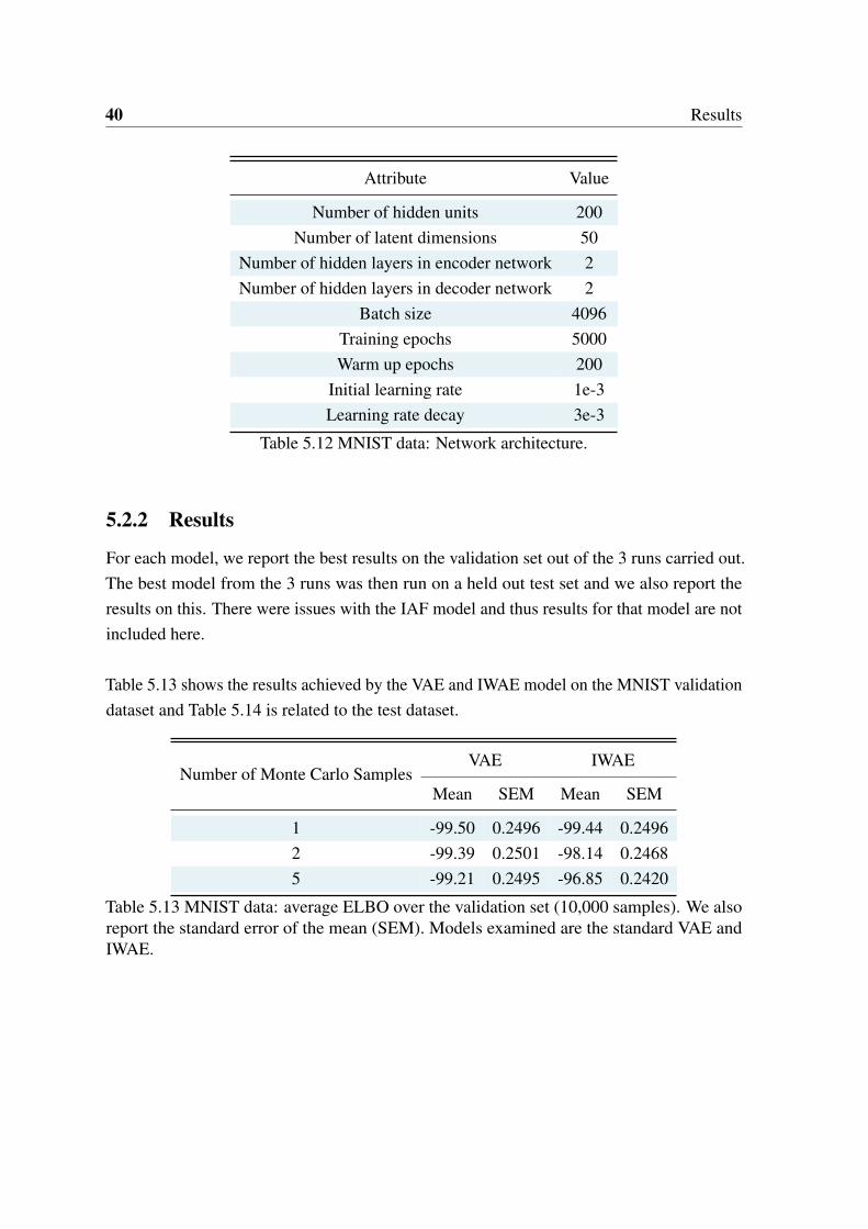
Table 5.12 MNIST data: Network architecture.

5.2.2 Results

For each model, we report the best results on the validation set out of the 3 runs carried out.The best model from the 3 runs was then run on a held out test set and we also report theresults on this. There were issues with the IAF model and thus results for that model are notincluded here.

Table 5.13 shows the results achieved by the VAE and IWAE model on the MNIST validationdataset and Table 5.14 is related to the test dataset.


Mean SEM Mean SEM

1 -99.50 0.2496 -99.44 0.24962 -99.39 0.2501 -98.14 0.24685 -99.21 0.2495 -96.85 0.2420

Table 5.13 MNIST data: average ELBO over the validation set (10,000 samples). We alsoreport the standard error of the mean (SEM). Models examined are the standard VAE andIWAE.



Mean SEM Mean SEM

1 -98.96 0.2518 -98.81 0.25252 -97.78 0.2518 -97.42 0.24795 -98.56 0.2507 -96.15 0.2420

Table 5.14 MNIST data: average ELBO over the test set (10,000 samples). We also reportthe standard error of the mean (SEM). Models examined are the standard VAE and IWAE.

Table 5.15 shows the results achieved by the ADGM and SDGM model on the MNISTvalidation dataset and Table 5.16 is related to the test dataset.


Mean SEM Mean SEM

1 -98.68 0.2509 -96.40 0.2480

Table 5.15 MNIST data: average ELBO over the validation set (10,000 samples). We alsoreport the standard error of the mean (SEM). Models examined are the ADGM and SDGM.


Mean SEM Mean SEM

1 -98.07 0.2523 -95.74 0.2493

Table 5.16 MNIST data: average ELBO over the test set (10,000 samples). We also reportthe standard error of the mean (SEM). Models examined are the ADGM and SDGM.

Table 5.17 shows the results achieved by the Householder model on the MNIST validationdataset and Table 5.18 is related to the test dataset.

42 Results


Mean SEM

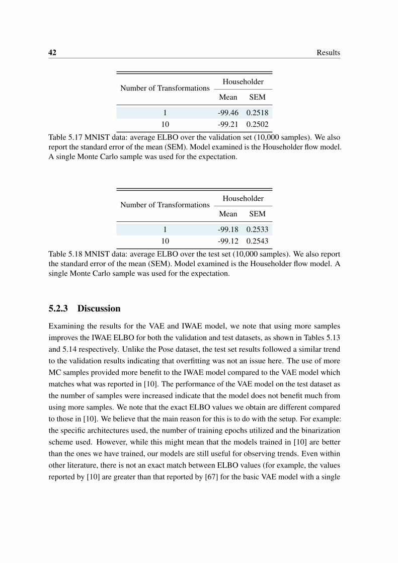
1 -99.46 0.251810 -99.21 0.2502

Table 5.17 MNIST data: average ELBO over the validation set (10,000 samples). We alsoreport the standard error of the mean (SEM). Model examined is the Householder flow model.A single Monte Carlo sample was used for the expectation.


Mean SEM

1 -99.18 0.253310 -99.12 0.2543

Table 5.18 MNIST data: average ELBO over the test set (10,000 samples). We also reportthe standard error of the mean (SEM). Model examined is the Householder flow model. Asingle Monte Carlo sample was used for the expectation.

5.2.3 Discussion

Examining the results for the VAE and IWAE model, we note that using more samplesimproves the IWAE ELBO for both the validation and test datasets, as shown in Tables 5.13and 5.14 respectively. Unlike the Pose dataset, the test set results followed a similar trendto the validation results indicating that overfitting was not an issue here. The use of moreMC samples provided more benefit to the IWAE model compared to the VAE model whichmatches what was reported in [10]. The performance of the VAE model on the test dataset asthe number of samples were increased indicate that the model does not benefit much fromusing more samples. We note that the exact ELBO values we obtain are different comparedto those in [10]. We believe that the main reason for this is to do with the setup. For example:the specific architectures used, the number of training epochs utilized and the binarizationscheme used. However, while this might mean that the models trained in [10] are betterthan the ones we have trained, our models are still useful for observing trends. Even withinother literature, there is not an exact match between ELBO values (for example, the valuesreported by [10] are greater than that reported by [67] for the basic VAE model with a single


MC sample by approximately 7 ELBO points).

Comparing the ADGM and SDGM model, we see that similar to the Pose data, the SDGMmodel outperforms the ADGM model as shown in Tables 5.15 and 5.16. Looking at the twoHouseholder setups examined, we see that using 10 transformations as opposed to just 1provides some improvement but not by a large margin for both the validation and test set.This lack of significant improvement was also observed in the original work by [67].

Next we consider all the models discussed in this section. Table 5.19 shows the resultsobtained on the MNIST validation set, ranked in order of degrading ELBO and Table 5.20reports similar data but for the test set.

Model ELBO Mean

SDGM -96.40IWAE (5 MC samples) -96.85IWAE (2 MC samples) -98.14

ADGM -98.68VAE (5 MC samples) -99.21

Householder (10 transformations) -99.21VAE (2 MC samples) -99.39IWAE (1 MC sample) -99.44

Householder (1 transformation) -99.46VAE (1 MC sample) -99.50

Table 5.19 MNIST data: average ELBO over the validation set (10,000 samples). A singleMonte Carlo sample was used for the expectation unless otherwise stated.

44 Results

Model ELBO Mean

SDGM -95.74IWAE (5 MC samples) -96.15IWAE (2 MC samples) -97.42VAE (2 MC samples) -97.78

ADGM -98.07Householder (10 transformations) -99.12Householder (1 transformation) -99.18

VAE (5 MC samples) -98.56IWAE (1 MC sample) -98.81VAE (1 MC sample) -98.96

Table 5.20 MNIST data: average ELBO over the test set (10,000 samples). A single MonteCarlo sample was used for the expectation unless otherwise stated.

Similar to the results for the Pose data, the SDGM model outperforms the other models. Weagain believe that this is due to explicitly modeling the latent space with a depth of 2. Forboth the validation and test set, the basic VAE model with a single sample performs the worst.This is expected as it has the weakest latent representation and does not have a tighter boundlike the IWAE model. We note that the range of ELBOs obtained here is much smaller thanthe results for the Pose data. This could be because the MNIST dataset is slightly easier tomodel and hence when more powerful models are used, the extra modeling capacity cannotbe put to full use because the dataset is too simple to leverage it. This may also explain whythe Householder model saw very little improvement when the number of transformations wasincreased. [67] also noted that using more transformations for the MNIST dataset yielded nosignificant improvement. However, as we showed in Section 5.1.3, for the Pose data, usingmore transformations yielded a large improvement. The lack of need for these more powerfulmodels with richer latent spaces, specifically the Householder model, can also be justified byobserving that the results obtained using the IWAE model with more than 1 MC sample werebetter than the Householder models for both the validation and test set.

Figure 5.2 shows an original sample from the MNIST test datasets and its reconstructionsunder some of the models.


(a) MNIST data: Original sample (b) MNIST data: VAE reconstruction

(c) MNIST data: IWAE reconstruction(d) MNIST data: Householder flow (1 trans-formation) reconstruction

(e) MNIST data: ADGM reconstruction (f) MNIST data: SDGM reconstruction

Fig. 5.2 MNIST data: A single sample from the testing dataset and its various reconstructionswith different models. All models only use a single Monte Carlo sample for expectations.

46 Results

5.3 celebA Likelihood

5.3.1 Architecture

For this dataset, we did not have expert help as was the case for the Pose data or a lotof VAE-specific literature to rely on as was the case for MNIST. So we ran a separateset of experiments to determine the best architecture. Specifically, we focused on thesehyper-parameters:

• Number of hidden units in each hidden layer

• Number of dimensions in the latent space

• Number of hidden layers in encoder and decoder network

Figure 5.3 shows the convergence plots for some of the cases we considered. To decide whichvalues to investigate, we considered previous work on the celebA dataset ([1, 11, 43]). Thedecreasing ELBO when 3 hidden layers were used in conjunction with 512 hidden units inthe encoder and decoder network show an issue with overfitting. Based on these experiments,we chose the following architecture:

Attribute Value




Initial learning rate 1e-3Learning rate decay 0

Table 5.21 celebA data: Network architecture.

5.3 celebA Likelihood 47

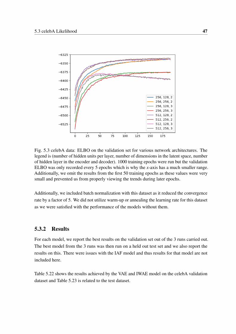
Fig. 5.3 celebA data: ELBO on the validation set for various network architectures. Thelegend is (number of hidden units per layer, number of dimensions in the latent space, numberof hidden layer in the encoder and decoder). 1000 training epochs were run but the validationELBO was only recorded every 5 epochs which is why the x-axis has a much smaller range.Additionally, we omit the results from the first 50 training epochs as these values were verysmall and prevented us from properly viewing the trends during later epochs.

Additionally, we included batch normalization with this dataset as it reduced the convergencerate by a factor of 5. We did not utilize warm-up or annealing the learning rate for this datasetas we were satisfied with the performance of the models without them.

5.3.2 Results

For each model, we report the best results on the validation set out of the 3 runs carried out.The best model from the 3 runs was then run on a held out test set and we also report theresults on this. There were issues with the IAF model and thus results for that model are notincluded here.

Table 5.22 shows the results achieved by the VAE and IWAE model on the celebA validationdataset and Table 5.23 is related to the test dataset.

48 Results


Mean SEM Mean SEM

1 -6336.33 4.33528 -6336.36 4.334682 -6335.54 4.33422 -6325.68 4.337585 -6334.39 4.33517 -6317.55 4.34009

Table 5.22 celebA data: average ELBO over the validation set (50,000 samples). We alsoreport the standard error of the mean (SEM). Models examined are the standard VAE andIWAE.


Mean SEM Mean SEM

1 -6331.26 4.32211 -6330.70 4.322622 -6330.17 4.32264 -6320.38 4.325935 -6329.27 4.32154 -6312.24 4.32703

Table 5.23 celebA data: average ELBO over the test set (50,000 samples). We also report thestandard error of the mean (SEM). Models examined are the standard VAE and IWAE.

Table 5.24 shows the results achieved by the ADGM and SDGM model on the celebAvalidation dataset and Table 5.25 is related to the test dataset.


Mean SEM Mean SEM

1 -6337.12 4.33327 -6316.63 4.33521

Table 5.24 celebA data: average ELBO over the validation set (10,000 samples). We alsoreport the standard error of the mean (SEM). Models examined are the ADGM and SDGM.



Mean SEM Mean SEM

1 6331.93 4.32050 -6311.40 4.32312

Table 5.25 celebA data: average ELBO over the test set (50,000 samples). We also report thestandard error of the mean (SEM). Models examined are the ADGM and SDGM.

Table 5.26 shows the results achieved by the Householder model on the celebA validationdataset and Table 5.27 is related to the test dataset.


Mean SEM

1 -6336.48 4.3377310 -6337.99 4.33879

Table 5.26 celebA data: average ELBO over the validation set (50,000 samples). We alsoreport the standard error of the mean (SEM). Model examined is the Householder flow model.A single Monte Carlo sample was used for the expectation.


Mean SEM

1 -6330.94 4.2348010 -6333.25 4.32553

Table 5.27 celebA data: average ELBO over the test set (50,000 samples). We also report thestandard error of the mean (SEM). Model examined is the Householder flow model. A singleMonte Carlo sample was used for the expectation.

5.3.3 Discussion

For this dataset, we will move straight to comparing the models overall as the trends shownin the individual Tables were very similar to that discussed with the MNIST dataset. Table5.28 shows the results obtained on the celebA validation set, ranked in order of worseningELBO and Table 5.29 reports similar results but for the test set.

50 Results

Model ELBO Mean

SDGM -6316.63IWAE (5 MC samples) -6317.55IWAE (2 MC samples) -6325.68VAE (5 MC samples) -6334.39VAE (2 MC samples) -6335.54VAE (1 MC sample) -6336.33

IWAE (1 MC sample) -6336.36Householder (1 transformation) -6336.48

ADGM -6337.12Householder (10 transformations) -6337.99

Table 5.28 celebA data: average ELBO over the validation set (50,000 samples). A singleMonte Carlo sample was used for the expectation unless otherwise stated.

Model ELBO Mean

SDGM -6311.40IWAE (5 MC samples) -6312.24IWAE (2 MC samples) -6320.38VAE (5 MC samples) -6329.27VAE (2 MC samples) -6330.17IWAE (1 MC sample) -6330.70

Householder (1 transformation) -6330.94VAE (1 MC sample) -6331.26

ADGM -6331.93Householder (10 transformations) -6333.25

Table 5.29 celebA data: average ELBO over the test set (50,000 samples). A single MonteCarlo sample was used for the expectation unless otherwise stated.

As was the case for the previous datasets, the SDGM model outperforms the other modelsinvestigated here. The most surprising results are perhaps the performance of the ADGMand Householder (with 10 transformations) model. For both the validation and test set, thesemodel perform worse than the basic VAE model. We believe that this is because this datasetis the most complex and hence some models require more fine-tuning than others. If this is


the case, then the SDGM, IWAE, and VAE models have an advantage in that they are ableto perform relatively well even without this fine tuning that the ADGM and Householdermodels may require.

While the celebA dataset is clearly more difficult to model, it does provide a better opportu-nity to compare models compared to the MNIST dataset. While the order of magnitude isdifferent, the range of ELBO values for the celebA dataset is much larger than MNIST whichhelps comparisons between the different models. The Pose dataset is the best option as itsorder of magnitude, for ELBO values, is smaller than celebA and comparable to MNISTwhile the range of ELBO values obtained is the largest of all 3 datasets.

While the results from the architecture experiments showed that we were not overfittingand the ELBO results discussed previously indicated that different models were achievingdiffering fits to the data, a qualitative analysis indicated that there were some issues withour models for the celebA dataset. Figure 5.4 shows reconstructions of a sample from thecelebA test dataset under our models. However, we found that the images shown appearedas the reconstruction for a range of test dataset inputs. This indicates that the models arecentered around a ’generic’ face that contains traits common to the dataset when it comes toreconstructing an image. While our architecture experiments indicated that a more powerfulmodel would be overfitting, these images indicate that our model still lacks capacity forimage reconstruction. One of the main differences of our work to previous works ([1, 11, 43])is that we did not used convolutional layers. Thus the most likely explanation is that thefeatures we were extracting from the image with our encoder network were insufficient forcompletely modeling the underlying manifold. However, these models did learn some of thenecessary traits of the celebA dataset required for image generation. Figure 5.5 shows imagesobtained by random sampling from the generative network. As we can see, in this instance,we are not limited to the same image. The variety here indicates that facial attributes werelearned and these models may be suitable for some generative tasks. The sample from theSDGM model indicates that this model has some issues but the ELBO associated with thevalidation and testing set for this model were reassuring. The images in Figure 5.4 indicatethat for reconstruction purposes, we need to reexamine our model architectures.

52 Results

(a) celebA data: VAE reconstruction (b) celebA data: IWAE reconstruction

(c) celebA data: ADGM reconstruction (d) celebA data: SDGM reconstruction

(e) celebA data: Householder flow (1 transfor-mation) reconstruction

(f) celebA data: Householder flow (10 trans-formations) reconstruction

Fig. 5.4 celebA data: Reconstruction of a single sample from the tests dataset under severalmodels. All models only use a single Monte Carlo sample for expectations.


(a) celebA data: VAE sample (b) celebA data: IWAE sample

(c) celebA data: ADGM sample (d) celebA data: SDGM sample

(e) celebA data: Householder flow (1 transfor-mation) sample

(f) celebA data: Householder flow (10 trans-formations) sample

Fig. 5.5 celebA data: Sampling from models. All models only use a single Monte Carlosample for expectations.

54 Results

5.4 Pose Timing

In this section, we examine how long key steps of the modeling process take. In particular, wewill consider how long a particular model takes to encode a data-point, decode a latent point,and update the network parameters. Additionally, for encoding and decoding, we considerthe time taken when using Chainer volatile and non-volatile variables. With non-volatilevariables, the history of operations used to create that variable is not stored. This preventsthat variable from being updated but also saves on memory usage. We record the timingson volatile and non-volatile variables to compare the difference in encoding and decodingbetween a training and testing scenario. This was done for 100 epochs and the average isreported along with the standard deviation.

5.4.1 Results

Number of Monte Carlo SamplesTraining Validation

Encoding Decoding Update Encoding Decoding

1 0.0076 (± 0.03913) 0.0036 (± 0.00101) 0.0095 (± 0.01733) 0.0035 (± 0.00033) 0.0035 (± 0.00177)2 0.0038 (± 0.00134) 0.0033 (± 0.00187) 0.0126 (± 0.00454) 0.0038 (± 0.00051) 0.0034 (± 0.00077)5 0.0036 (± 0.00188) 0.0034 (± 0.00047) 0.0245 (± 0.00350) 0.0033 (± 0.00213) 0.0033 (± 0.00068)

Table 5.30 Pose data: average times over the training and validation set (351,275 and 175,638samples respectively). We also report the standard deviation in brackets. Model examined isthe VAE.



1 0.0037 (± 0.00129) 0.0034 (± 0.00018) 0.0087 (± 0.00074) 0.0034 (± 0.00033) 0.0033 (± 0.00070)2 0.0037 (± 0.00142) 0.0033 (± 0.00028) 0.0154 (± 0.00150) 0.0036 (± 0.00052) 0.0034 (± 0.00059)5 0.0037 (± 0.00138) 0.0033 (± 0.00026) 0.0325 (± 0.00278) 0.0037 (± 0.00106) 0.0033 (± 0.00041)

Table 5.31 Pose data: average times over the training and validation set (351,275 and 175,638samples respectively). We also report the standard deviation in brackets. Model examined isthe IWAE.

5.4 Pose Timing 55

ModelTraining Validation


ADGM 0.0086 (± 0.01838) 0.0065 (± 0.00203) 0.2474 (± 0.00306) 0.0069 (± 0.00060) 0.0065 (± 0.00077)SDGM 0.0068 (± 0.00198) 0.0064 (± 0.00452) 0.2467 (± 0.00330) 0.0070 (± 0.00058) 0.0065 (± 0.00051)

Table 5.32 Pose data: average times over the training and validation set (351,275 and 175,638samples respectively). We also report the standard deviation in brackets. Models examinedare the ADGM and SDGM. A single Monte Carlo sample was used for the expectation.

Number of TransformationsTraining Validation


1 0.0041 (± 0.00126) 0.0073 (± 0.01774) 0.0110 (± 0.00132) 0.0039 (± 0.00101) 0.0051 (± 0.00095)10 0.0046 (± 0.00498) 0.0229 (± 0.01109) 0.0220 (± 0.00825) 0.0036 (± 0.00342) 0.0182 (± 0.01264)

Table 5.33 Pose data: average times over the training and validation set (351,275 and 175,638samples respectively). We also report the standard deviation in brackets. Model examined isthe Householder flow. A single Monte Carlo sample was used for the expectation.



1 0.0040 (± 0.00171) 0.0077 (± 0.00068) 0.0102 (± 0.00152) 0.0036 (± 0.00144) 0.0074 (± 0.00220)2 0.0044 (± 0.00654) 0.0107 (± 0.00801) 0.0123 (± 0.01152) 0.0025 (± 0.01193) 0.0091 (± 0.00970)3 0.0028 (± 0.00913) 0.0128 (± 0.01430) 0.0117 (± 0.01518) 0.0041 (± 0.01632) 0.0114 (± 0.01879)4 0.0041 (± 0.00183) 0.0169 (± 0.00154) 0.1326 (± 0.00275) 0.0038 (± 0.00081) 0.0150 (± 0.00168)8 0.0041 (± 0.00140) 0.0277 (± 0.00203) 0.1397 (± 0.00293) 0.0038 (± 0.00131) 0.0255 (± 0.00335)

Table 5.34 Pose data: average times over the training and validation set (351,275 and 175,638samples respectively). We also report the standard deviation in brackets. Model examined isthe IAF. A single Monte Carlo sample was used for the expectation.

5.4.2 Discussion

We first consider the times taken by the VAE and IWAE models, shown in Table 5.30 and5.31. As they have the same architectures, it is not surprising to see that the time taken toencode a data-point for both these models is approximately the same. This same can beobserved for the time taken to decode latent points. We note that this time is averaged acrossthe number of MC samples used which is why there isn’t any significant increase in time asthe number of MC samples is increased.

For both the VAE and IWAE model, we observe that the time taken to update the networkparameters increases as the number of MC samples used increases. Using more samples

56 Results

results in a more complex computational graph and this results in a more involved backprop-agation update procedure. As the update procedure takes into account the loss function orELBO being used, we can compare differences between the VAE and IWAE here. Usingonly a single MC sample, the IWAE objective is almost the same as the VAE objective. Theonly difference for this case is that with the VAE, we evaluate the KL divergence analyticallybut for the IWAE, we use expectations. In our code, the analytic KL is implemented as aseparate function whereas for the IWAE, it is evaluated closer to the other operations. Thismay explain why the update time is longer for the VAE compared to the IWAE when onlya single MC sample is used. When using 2 or 5 MC samples, the complexity of the IWAEELBO comes into play and we see that for both theses cases, updates take longer comparedto the VAE.

It is also interesting to note that while non-volatile variables consume less memory and henceshould be faster to encode and decode, we observe no difference. If the data-points andlatent points had more dimensions or if we used larger batch sizes, perhaps a differencewould show since we would be increasing the memory consumption. However, for ourinvestigation into the VAE and IWAE models on the Pose dataset, there was no differencebetween using volatile and non-volatile variables with respect to encoding and decoding time.

Next we consider the timings recorded for the ADGM and SDGM models, as shown in Table5.32. We begin by noting that the times taken to encode are similar whether using volatileor non-volatile variables, for both the models. The only value that is a little higher thanthe others is the volatile encoding time for the ADGM. However, the significantly higherstandard deviation means that this measure may not be a good representative for the averageADGM encoding time. Once again, the update timings hold more interesting information.If we consider their probabilistic models, they both have the same variables with the keydifference being in how these variables relate to each other. Therefore, from a networkperspective, the number of parameters in both networks is approximately the same and witha single MC sample, so is the number of computations. As a result, their update times areapproximately the same.

For the Householder flow model, we defined the encoding process to only encapsulate thetime taken to go from the original data-point to the basic latent space, z0. This is why thetime taken to encode is approximately the same whether a single transformation or 10 areused as shown in Table 5.33. The additional transformation or flows are timed as part of thedecoding process and hence we see that for both the training and validation set, there is an

5.4 Pose Timing 57

increase in decoding time when more transformations are used. Note that even though 9 moretransformations are used, we don’t see the time increase by a factor of 10. This is becausethere are operations involved in the decoding process that are present in the same amountregardless of how many transformations are used. Specifically, after the latent point hasbeen transformed, it must be pushed through the decoder network to obtain the reconstructeddata-point. This aspect of the decoding process will occur in the same manner regardlessof how many flows were applied to transform the latent point. Additionally, as more flowsare used, there are more operations involved which leads to a longer update period. Notethat with the Householder flow, the same linear layer is used to obtain a new Householdervector for each flow. This means that more flows don’t change the number of parameters ofthe network. The longer update time is due to the increase in number of operations, not thenumber of parameters.

Considering the IAF models, the same idea was applied to timing the encoding and decodingprocedure as was done with the Householder model. The encoding procedure times howlong it takes to encode a data-point to the basic latent space. The decoding time covers thetime taken to apply the auto-regressive flows to the first latent point and also the time takento decode the final latent point to the reconstructed data-point. Hence we see the encodingtime remain approximately the same regardless of how many flows are used while the decod-ing time increases as more flows are applied. For the IAF model, each transformations iscategorized by a different set of parameters. Therefore the increase in update time is due toboth an increase in the number of operations in the gradient calculation and also an increasein the number of parameters to update.

Having considered the different models in relative isolation, we now compare the timingsacross all the models on the Pose data. Firstly, encoding takes about the same amount of timefor the different models. The only two models that have a longer encoding procedure are theADGM and SDGM. However, these models have an additional variable in the probabilisticmodel. This additional variable and the parameters associated with it would explain why theencoding procedure for the ADGM and SDGM take much longer than the other models.

Next, we examine the decoding procedure across these different models. The VAE and IWAEmodels have the fastest times here as they have the simplest decoding procedure. The ADGMand SDGM also have fairly standard decoding procedures, in that they do not have to considernumber of transformations or flows like the Householder or IAF model. However, as both theADGM and SDGM have more complex generative models, their decoding procedures are also

58 Results

more involved. As a result, their decoding takes significantly longer than the VAE or IWAE.As mentioned previously, for the Householder and IAF model, using more transformationsincreases the decoding time. However, even with just a single transformation, these modelstake longer to decode compared to the other models. If we compare the time taken to decodefor the Householder model against the IAF model, we see that IAF transformations are morecostly in terms of time. Using 8 IAF transformations takes longer than using 10 Householderflow transformations. Hence when it comes to decoding, the IAF model has the highest cost.

Following on, we look at the time taken to update the model after a batch has been processed.This metric is very informative as it relates to the computational graph of each model andhence the complexity of these models. It can also act as a proxy as to how many parametersa particular configuration has. The higher the number of parameters, the longer the updateprocedure will take. This may not always be the case and we elaborate on this further on.Firstly, given a single MC sample, we see that the the VAE and IWAE models take a shortertime to update than the other models. As previously noted, these models have the simplestarchitectures and hence it is unsurprising that these models update quickly, relative to theother models. Even though the ADGM and SDGM may have less network parameters andless operations compared to the flow models, the underlying probabilistic model is morecomplex and hence these two models have a very high update time. Comparing the flow mod-els, we see that the update time increases at a much faster rate for the IAF model comparedto the Householder flow model as more transformations are added. As previously mentioned,more transformations with the Householder flow do not lead to more parameters unlike theIAF. Thus when increasing the number of transformations with an IAF model, the number ofoperations and number of parameters increases leading to a larger update time compared tothe Householder flow model in which only the number of operations increases. Overall, theADGM and SDGM model have the highest base update time. We include the term ’base’ asit is possible that by using an even higher number of transformations with the Householderflow or IAF model compared to what was considered here, their respective update timesmight exceed that of the ADGM and SDGM.

5.5 MNIST Timing 59

5.5 MNIST Timing

5.5.1 Results



1 0.0020 (± 0.00224) 0.0014 (± 0.00007) 0.0133 (± 0.00180) 0.0018 (± 0.00024) 0.0014 (± 0.00014)2 0.0019 (± 0.00222) 0.0013 (± 0.00051) 0.0198 (± 0.00148) 0.0017 (± 0.00007) 0.0013 (± 0.00004)5 0.0020 (± 0.00227) 0.0013 (± 0.00034) 0.0395 (± 0.00196) 0.0017 (± 0.00009) 0.0013 (± 0.00006)

Table 5.35 MNIST data: average times over the training and validation set (50,000 and10,000 samples respectively). We also report the standard deviation in brackets. Modelexamined is the VAE.



1 0.0020 (± 0.00212) 0.0013 (± 0.00060) 0.0132 (± 0.00141) 0.0018 (± 0.00024) 0.0013 (± 0.00005)2 0.0020 (± 0.00218) 0.0014 (± 0.00007) 0.0198 (± 0.00182) 0.0017 (± 0.00006) 0.0014 (± 0.00005)5 0.0019 (± 0.00236) 0.0014 (± 0.00004) 0.0395 (± 0.00231) 0.0017 (± 0.00015) 0.0014 (± 0.00011)

Table 5.36 MNIST data: average times over the training and validation set (50,000 and10,000 samples respectively). We also report the standard deviation in brackets. Modelexamined is the IWAE.



ADGM 0.0039 (± 0.00226) 0.0031 (± 0.00091) 0.0257 (± 0.00180) 0.0031 (± 0.00386) 0.0031 (± 0.00010)SDGM 0.0036 (± 0.00238) 0.0032 (± 0.00067) 0.0241 (± 0.00149) 0.0036 (± 0.00012) 0.0028 (± 0.00393)

Table 5.37 MNIST data: average times over the training and validation set (50,000 and 10,000samples respectively). We also report the standard deviation in brackets. Models examinedare the ADGM and SDGM. A single Monte Carlo sample was used for the expectation.



1 0.0022 (± 0.00220) 0.0028 (± 0.00043) 0.0211 (± 0.00136) 0.0020 (± 0.00022) 0.0027 (± 0.00020)10 0.0022 (± 0.00166) 0.0158 (± 0.00169) 0.0789 (± 0.00308) 0.0020 (± 0.00026) 0.0152 (± 0.00158)

Table 5.38 MNIST data: average times over the training and validation set (50,000 and 10,000samples respectively). We also report the standard deviation in brackets. Model examined isthe Householder flow. A single Monte Carlo sample was used for the expectation.

60 Results

5.5.2 Discussion

For most of the models, we observe the same trends and behaviours for the MNIST datasetas was seen with the Pose data. There are a few subtle differences between the results onthese two datasets. To begin with, the models took longer to encode and decode the Posedatasets compared to MNIST. We believe that this is due to the size of the mini-batches beingused. Preliminary experiments showed that the GPU processes ran slower when the loadwas higher, even if the entire capacity of the GPU was not being utilized. With the Posetiming experiments, we used a batch size of 16,384 whereas with MNIST, we used 4,096.The larger batch size of the Pose data appears to have taken slightly longer to encode anddecode compared to the MNIST dataset. It is also interesting to note that the batch sizeseemed to have a greater effect that the dimensionality of the data since with MNIST, thedimensionality of the original data-points and the dimensionality of the latent space were fargreater compared to their respective counterparts in the Pose dataset. However, while usinglarger batches incurs a small time cost, the time saved from having to process less batches isfar greater. Therefore, to minimize the overall time overhead, large batch sizes should beused despite having a longer encoding and decoding process per batch.

We see that the VAE and IWAE model take less time to encode, decode, and update due totheir simpler architectures. Additionally, the difference in update time between the VAEand IWAE are much smaller here. We believe that this is because the batch sizes weresignificantly smaller. A larger batch size will likely show the IWAE model taking longerthan the VAE model as more MC samples are used. While the ADGM and SDGM havelarge base times, we see that if we use 10 Householder flow transformations, the decod-ing and update time of the Householder model is greater than those of the ADGM and SDGM.

5.6 celebA Timing 61

5.6 celebA Timing

5.6.1 Results



1 0.0038 (± 0.00210) 0.0029 (± 0.00005) 0.1953 (± 0.00069) 0.0036 (± 0.00009) 0.0028 (± 0.00006)2 0.0036 (± 0.00186) 0.0028 (± 0.00011) 0.3233 (± 0.02761) 0.0034 (± 0.00015) 0.0027 (± 0.00010)5 0.0040 (± 0.00073) 0.0048 (± 0.00070) 0.6652 (± 0.00088) 0.0040 (± 0.00024) 0.0032 (± 0.00018)

Table 5.39 celebA data: average times over the training and validation set (100,000 and50,000 samples respectively). We also report the standard deviation in brackets. Modelexamined is the VAE.



1 0.0037 (± 0.00204) 0.0029 (± 0.00006) 0.1954 (± 0.00086) 0.0035 (± 0.00007) 0.0028 (± 0.00005)2 0.0037 (± 0.00199) 0.0029 (± 0.00005) 0.3136 (± 0.00099) 0.0035 (± 0.00007) 0.0028 (± 0.00006)5 0.0037 (± 0.00207) 0.0030 (± 0.00007) 0.6672 (± 0.00081) 0.0035 (± 0.00010) 0.0028 (± 0.00006)

Table 5.40 celebA data: average times over the training and validation set (100,000 and50,000 samples respectively). We also report the standard deviation in brackets. Modelexamined is the IWAE.



ADGM 0.0071 (± 0.00204) 0.0062 (± 0.00011) 0.3307 (± 0.00095) 0.0069 (± 0.00015) 0.0061 (± 0.00012)SDGM 0.0072 (± 0.00291) 0.0062 (± 0.00012) 0.2837 (± 0.00069) 0.0069 (± 0.00016) 0.0061 (± 0.00011)

Table 5.41 celebA data: average times over the training and validation set (100,000 and50,000 samples respectively). We also report the standard deviation in brackets. Modelsexamined are the ADGM and SDGM. A single Monte Carlo sample was used for theexpectation.



1 0.0039 (± 0.00208) 0.0043 (± 0.00037) 0.2193 (± 0.00074) 0.0037 (± 0.00007) 0.0041 (± 0.00008)10 0.0037 (± 0.00216) 0.0158 (± 0.00075) 0.3907 (± 0.00078) 0.0035 (± 0.00022) 0.0151 (± 0.00047)

Table 5.42 celebA data: average times over the training and validation set (100,000 and50,000 samples respectively). We also report the standard deviation in brackets. Modelexamined is the Householder flow. A single Monte Carlo sample was used for the expectation.

62 Results

5.6.2 Discussion

The celebA dataset was the largest dataset considered in terms of disk space usage. Themachine used to run the timing experiments for the Pose and MNIST datasets was too smallto keep the celebA dataset on disk. Therefore, timing experiments for the celebA datasetwere run on a different machine with a different GPU. As such, we cannot make directcomparisons between the times recorded for the celebA dataset against those for the Poseand MNIST datasets. However, the results gathered are still useful for checking if the trendsobserved when timing the Pose and MNIST dataset experiments still hold. In general, thesame trends are observed. The VAE and IWAE model take the least amount of time to encode,decode, and update. While the ADGM and SDGM take a lot of time, if a sufficient numberof Householder flow transformations are applied, the decoding and update time taken by theHouseholder model exceeds that of the ADGM and SDGM.

5.7 Practical Recommendations

In the previous sections, we discussed the modeling capacity of each of our models as well asthe time costs associated with them. The SDGM performed consistently well across all taskswith regards to ELBO but often took significantly longer to carry out its operations (encode,decode and update) as opposed to the other options. For the Pose data, we recommend theIAF as it performed the best and had smaller training times, even with 8 transformations,relative to other models like the SDGM. Computational resources permitting, we recommendusing more transformations.

While the SDGM model had the best ELBO on the MNIST and celebA datasets, the IWAEmodel with 5 MC samples also performed very well while having shorter encoding anddecoding times. On the MNIST dataset, the ELBO gap between the SDGM and IWAE 5 MCmodel is small enough that if fast models were a priority, both from a training and samplingperspective, the IWAE 5 MC model would be a good option. We observe that for the updateprocedure on the celebA dataset, the SDGM model requires less time compared to the IWAE5 MC model which makes the SDGM more favourable in this situation. Speaking moregenerally, the IWAE model requires more samples to achieve a better fit but the increasedupdate time cost associated with this is strongly linked to the dataset being modeled. For lowdimensional data like MNIST, we see that the update time doesn’t increase much as moreMC samples are used but for higher dimensional data like celebA, we see the update timeincrease at a much faster rate. This is not as big an issue with the SDGM model since it iscapable of achieving good fits without using more than 1 MC sample. If small training and

5.7 Practical Recommendations 63

sampling times are not a priority, we recommend using the SDGM. However, if these arebigger priorities than the ELBO, we recommend considering the IWAE model. Choosingthe right setup with the IWAE model may be more involved as we have to consider thedimensionality of the data and choose the appropriate number of MC samples. More MCsamples will lead to a better ELBO but at some point, the time savings that were importantare lost.

Chapter 6

Summary and Future Work

6.1 Summary

In conclusion, we believe that we achieved the aims of this project. In Chapter 5, weprovided a thorough comparison of several modifications to the Variational Auto-Encoder(VAE) ([31, 54]). We measured the variational lower bound as is common to most of theliterature but additionally we reported the time taken for different stages of the modelingprocess. Using both these metrics, in Section 5.7, we offered practical guidelines on thewhich models might be best suited for different tasks. Additionally, while most related workfocuses on MNIST, we also looked at two different datasets: celebA and Pose (MSRC-12).By showing recurring trends across three significantly different datasets, we are able tostate our conclusions with more confidence. On top of this, we have also contributed anextensive Chainer code repository ([16]) to allow others access to these new probabilisticdeep generative models and to replicate our experiments.

6.2 Future Work and Extensions

6.2.1 Inverse Autoregressive Flow on other datasets

We were unable to obtain results for the Inverse Autoregressive Flow (IAF) model on theMNIST and celebA datasets. While we could draw some conclusions about this model basedon its performance on the Pose dataset, [33] claimed that one of the main strengths of theIAF model was its ability to handle high dimensional latent spaces. Of the datasets examined,the Pose dataset involved the latent space with the smallest dimension, compared to MNISTand celebA. To fully examine the capabilities of the IAF model, we believe that it will benecessary to examine its performance on datasets requiring large latent spaces.

66 Summary and Future Work

6.2.2 Planar Flow model

We attempted to implement the Planar flow model which was the focus of [53] but wereunsuccessful. Our attempted implementation has been included in the aforementioned repos-itory. We believe that this is another important model to investigate as it was one of thefirst normalizing flow methods examined. It would be especially useful to compare theperformance of this model against that of the Householder flow and IAF models as theselatter two are more recent normalizing flow models.

Specifically, [33] claimed that the Planar flow model was analogous to a multi-layer percep-tron bottleneck and would perform poorly when handling high-dimensional latent spaceswhereas the IAF overcame this issue. It would be useful to test this claim, specifically to deter-mine at which point the latent space became too large to be modeled by the Planar flow model.

The Householder flow model by [67] is an example of a volume preserving normalizingflow as opposed to the Planar flow model which is a general normalizing flow model. Theformer is cheaper than the latter and by implementing the Planar flow model, we would bebetter able to consider the trade-off between computational complexity and accuracy betweengeneral and volume preserving normalizing flows.

6.2.3 Timing of celebA dataset

As mentioned in Section 5.6.2, due to the size of the celebA dataset, a different machine hadto be used to carry out the timing experiments compared to the Pose and MNIST datasets.It would be beneficial to redo the celebA timing experiments using the same GPU modelused for the other datasets but with a machine with enough disk space to store the dataset.The results of this would provide more insight into the relationship between timing and datadimensionality as the celebA dataset datapoints were of a much larger dimension than thePose and MNIST datasets.

6.2.4 Fine-tuning models

In this work, none of the model architectures were fine-tuned extensively. For the Poseand MNIST datasets, related work informed our model choice. For the celebA dataset, weconsidered the literature and performed experiments with the validation dataset and the VAEmodel to determine the best architecture choice. However, to better measure the capacity

6.2 Future Work and Extensions 67

of each model, we should instead carry out the architecture experiments on the validationdataset for each model individually. In this work, we assumed that the architecture andsettings used for the VAE model were also suitable for the other models but this might notnecessarily be true. We do not believe that in being more thorough with the architecturechoice, the results obtained and trends observed will be significantly different but instead, wecould be more secure about our observations and recommendations.

6.2.5 Convolutional layers

As discussed in Section 5.3.3, our models encountered difficulty in reconstructing imagesfrom the celebA test dataset even though sampling from the generative network indicatedthat facial attributes were being learned. To overcome this issue, we would recommendexperimenting with convolutional layers instead of fully connected layers. These layers haveshown a lot of promise in extracting meaningful features for complex image data ([34, 52]).

6.2.6 Depth in stochastic layers

One model that performed consistently well across all the datasets was the Skip Deep Gen-erative Model (SDGM). As mentioned in Section 5.1.3, we believe that this is due to thedepth in the stochastic layer. Having more than one layer in the latent space is not somethingunique to the SDGM. Hence it would be worthwhile to increase the stochastic depth for theother models and examine the resulting performance. Such an undertaking would provideclearer understanding into the importance and limitations of increasing the depth of the latentspace.

References

[1] S. Agrawal and A. Dukkipati. Deep variational inference without pixel-wise reconstruc-tion. arXiv preprint arXiv:1611.05209, 2016.

[2] Y. Bengio. Neural net language models. Scholarpedia, 3(1):3881, 2008.

[3] Y. Bengio, Y. LeCun, et al. Scaling learning algorithms towards ai. Large-scale kernelmachines, 34(5):1–41, 2007.

[4] Y. Bengio, A. Courville, and P. Vincent. Representation learning: A review and newperspectives. IEEE transactions on pattern analysis and machine intelligence, 35(8):1798–1828, 2013.

[5] M. Bicego, A. Lagorio, E. Grosso, and M. Tistarelli. On the use of sift features forface authentication. In Computer Vision and Pattern Recognition Workshop, 2006.CVPRW’06. Conference on, pages 35–35. IEEE, 2006.

[6] A. W. Black. Clustergen: A statistical parametric synthesizer using trajectory modeling.In Ninth International Conference on Spoken Language Processing, 2006.

[7] D. M. Blei. Variational inference.

[8] D. M. Blei, A. Kucukelbir, and J. D. McAuliffe. Variational inference: A review forstatisticians. Journal of the American Statistical Association, (just-accepted), 2017.

[9] A. E. Bryson. Applied optimal control: optimization, estimation and control. CRCPress, 1975.

[10] Y. Burda, R. Grosse, and R. Salakhutdinov. Importance weighted autoencoders. arXivpreprint arXiv:1509.00519, 2015.

[11] L. Cai, H. Gao, and S. Ji. Multi-stage variational auto-encoders for coarse-to-fine imagegeneration. arXiv preprint arXiv:1705.07202, 2017.

[12] Chervinskii. Auto-encoder structure, 2015. URL https://commons.wikimedia.org/wiki/File:Autoencoder_structure.png.

[13] D. Ciregan, U. Meier, and J. Schmidhuber. Multi-column deep neural networks forimage classification. In Computer Vision and Pattern Recognition (CVPR), 2012 IEEEConference on, pages 3642–3649. IEEE, 2012.

https://commons.wikimedia.org/wiki/File:Autoencoder_structure.png

https://commons.wikimedia.org/wiki/File:Autoencoder_structure.png

70 References

[14] D. C. Ciresan, U. Meier, L. M. Gambardella, and J. Schmidhuber. Deep, big, simpleneural nets for handwritten digit recognition. Neural computation, 22(12):3207–3220,2010.

[15] C. Cremer, Q. Morris, and D. Duvenaud. Reinterpreting importance-weighted autoen-coders. arXiv preprint arXiv:1704.02916, 2017.

[16] A. D. D’Cruz. Deep generative models. https://github.com/ashwindcruz/dgm, 2017.

[17] C. Doersch. Tutorial on variational autoencoders. arXiv preprint arXiv:1606.05908,2016.

[18] J. Duchi, E. Hazan, and Y. Singer. Adaptive subgradient methods for online learning andstochastic optimization. Journal of Machine Learning Research, 12(Jul):2121–2159,2011.

[19] S. Fothergill, H. Mentis, P. Kohli, and S. Nowozin. Instructing people for traininggestural interactive systems. In Proceedings of the SIGCHI Conference on HumanFactors in Computing Systems, pages 1737–1746. ACM, 2012.

[20] K. Fukushima and S. Miyake. Neocognitron: A self-organizing neural network modelfor a mechanism of visual pattern recognition. In Competition and cooperation inneural nets, pages 267–285. Springer, 1982.

[21] M. Gales. 4f10 deep learning. 2016. URL http://mi.eng.cam.ac.uk/~mjfg/local/4F10/index.html.

[22] T. Ganchev, N. Fakotakis, and G. Kokkinakis. Comparative evaluation of various mfccimplementations on the speaker verification task. In Proceedings of the SPECOM,volume 1, pages 191–194, 2005.

[23] M. Germain, K. Gregor, I. Murray, and H. Larochelle. Made: masked autoencoderfor distribution estimation. In Proceedings of the 32nd International Conference onMachine Learning (ICML-15), pages 881–889, 2015.

[24] Z. Ghahramani. Unsupervised learning. In Advanced lectures on machine learning,pages 72–112. Springer, 2004.

[25] X. Hou, L. Shen, K. Sun, and G. Qiu. Deep feature consistent variational autoencoder.In Applications of Computer Vision (WACV), 2017 IEEE Winter Conference on, pages1133–1141. IEEE, 2017.

[26] D. H. Hubel and T. N. Wiesel. Receptive fields, binocular interaction and functionalarchitecture in the cat’s visual cortex. The Journal of physiology, 160(1):106–154,1962.

[27] S. Ioffe and C. Szegedy. Batch normalization: Accelerating deep network training byreducing internal covariate shift. In International Conference on Machine Learning,pages 448–456, 2015.

[28] E. Jang. A beginner’s guide to variational methods: Mean-field approximation, 2016.URL http://blog.evjang.com/2016/08/variational-bayes.html.

https://github.com/ashwindcruz/dgm

http://mi.eng.cam.ac.uk/~mjfg/local/4F10/index.html

http://mi.eng.cam.ac.uk/~mjfg/local/4F10/index.html

http://blog.evjang.com/2016/08/variational-bayes.html

References 71

[29] A. Karpathy. Cs231n convolutional neural networks for visual recognition, 2017. URLhttp://cs231n.github.io.

[30] D. Kingma and J. Ba. Adam: A method for stochastic optimization. arXiv preprintarXiv:1412.6980, 2014.

[31] D. P. Kingma and M. Welling. Auto-encoding variational bayes. arXiv preprintarXiv:1312.6114, 2013.

[32] D. P. Kingma, S. Mohamed, D. J. Rezende, and M. Welling. Semi-supervised learningwith deep generative models. In Advances in Neural Information Processing Systems,pages 3581–3589, 2014.

[33] D. P. Kingma, T. Salimans, and M. Welling. Improving variational inference withinverse autoregressive flow. arXiv preprint arXiv:1606.04934, 2016.

[34] A. Krizhevsky, I. Sutskever, and G. E. Hinton. Imagenet classification with deepconvolutional neural networks. In Advances in neural information processing systems,pages 1097–1105, 2012.

[35] H. Larochelle, D. Erhan, A. Courville, J. Bergstra, and Y. Bengio. An empirical evalua-tion of deep architectures on problems with many factors of variation. In Proceedingsof the 24th international conference on Machine learning, pages 473–480. ACM, 2007.

[36] A. B. L. Larsen, S. K. Sønderby, H. Larochelle, and O. Winther. Autoencoding beyondpixels using a learned similarity metric. arXiv preprint arXiv:1512.09300, 2015.

[37] Y. LeCun. The mnist database of handwritten digits. http://yann. lecun. com/exdb/mnist/,1998.

[38] Y. LeCun, Y. Bengio, and G. Hinton. Deep learning. Nature, 521(7553):436–444, 2015.

[39] Z. Liu, P. Luo, X. Wang, and X. Tang. Deep learning face attributes in the wild. InProceedings of International Conference on Computer Vision (ICCV), 2015.

[40] L. Maaløe, C. K. Sønderby, S. K. Sønderby, and O. Winther. Auxiliary deep generativemodels. arXiv preprint arXiv:1602.05473, 2016.

[41] D. J. MacKay. Local minima, symmetry-breaking, and model pruning in variationalfree energy minimization. Inference Group, Cavendish Laboratory, Cambridge, UK,2001.

[42] W. S. McCulloch and W. Pitts. A logical calculus of the ideas immanent in nervousactivity. Bulletin of mathematical biology, 52(1):99–115, 1990.

[43] L. Mescheder, S. Nowozin, and A. Geiger. Adversarial variational bayes: Unify-ing variational autoencoders and generative adversarial networks. arXiv preprintarXiv:1701.04722, 2017.

[44] Microsoft. Msrc-12, 2012. URL https://www.microsoft.com/en-us/download/details.aspx?id=52283.

http://cs231n.github.io

https://www.microsoft.com/en-us/download/details.aspx?id=52283

https://www.microsoft.com/en-us/download/details.aspx?id=52283

72 References

[45] V. Nair and G. E. Hinton. Rectified linear units improve restricted boltzmann machines.In Proceedings of the 27th international conference on machine learning (ICML-10),pages 807–814, 2010.

[46] K. S. Narendra and M. A. Thathachar. Learning automata-a survey. IEEE Transactionson systems, man, and cybernetics, (4):323–334, 1974.

[47] M. A. Nielsen. Chapter 2: How the backpropagation algorithm works. DeterminationPress, 2015. URL http://neuralnetworksanddeeplearning.com/chap2.html.

[48] A. v. d. Oord, S. Dieleman, H. Zen, K. Simonyan, O. Vinyals, A. Graves, N. Kalch-brenner, A. Senior, and K. Kavukcuoglu. Wavenet: A generative model for raw audio.arXiv preprint arXiv:1609.03499, 2016.

[49] A. v. d. Oord, N. Kalchbrenner, and K. Kavukcuoglu. Pixel recurrent neural networks.arXiv preprint arXiv:1601.06759, 2016.

[50] J. Paisley, D. Blei, and M. Jordan. Variational bayesian inference with stochastic search.arXiv preprint arXiv:1206.6430, 2012.

[51] C. Poultney, S. Chopra, Y. L. Cun, et al. Efficient learning of sparse representationswith an energy-based model. In Advances in neural information processing systems,pages 1137–1144, 2007.

[52] A. Radford, L. Metz, and S. Chintala. Unsupervised representation learning with deepconvolutional generative adversarial networks. arXiv preprint arXiv:1511.06434, 2015.

[53] D. J. Rezende and S. Mohamed. Variational inference with normalizing flows. arXivpreprint arXiv:1505.05770, 2015.

[54] D. J. Rezende, S. Mohamed, and D. Wierstra. Stochastic backpropagation and approxi-mate inference in deep generative models. arXiv preprint arXiv:1401.4082, 2014.

[55] F. Rosenblatt. The perceptron: A probabilistic model for information storage andorganization in the brain. Psychological review, 65(6):386, 1958.

[56] D. E. Rumelhart, G. E. Hinton, and R. J. Williams. Learning internal representationsby error propagation. Technical report, California Univ San Diego La Jolla Inst forCognitive Science, 1985.

[57] R. Salakhutdinov. Learning deep generative models. University of Toronto, 2009.

[58] J. Schmidhuber. Deep learning in neural networks: An overview. Neural networks, 61:85–117, 2015.

[59] F. Seide, G. Li, and D. Yu. Conversational speech transcription using context-dependentdeep neural networks. In Twelfth Annual Conference of the International SpeechCommunication Association, 2011.

[60] W. Shang, K. Sohn, D. Almeida, and H. Lee. Understanding and improving convolu-tional neural networks via concatenated rectified linear units. CoRR, abs/1603.05201,2016. URL http://arxiv.org/abs/1603.05201.

http://neuralnetworksanddeeplearning.com/chap2.html

http://arxiv.org/abs/1603.05201

References 73

[61] P. Y. Simard, D. Steinkraus, J. C. Platt, et al. Best practices for convolutional neuralnetworks applied to visual document analysis. In ICDAR, volume 3, pages 958–962,2003.

[62] C. K. Sønderby, T. Raiko, L. Maaløe, S. K. Sønderby, and O. Winther. How totrain deep variational autoencoders and probabilistic ladder networks. arXiv preprintarXiv:1602.02282, 2016.

[63] E. Tabak and C. V. Turner. A family of nonparametric density estimation algorithms.Communications on Pure and Applied Mathematics, 66(2):145–164, 2013.

[64] E. G. Tabak, E. Vanden-Eijnden, et al. Density estimation by dual ascent of thelog-likelihood. Communications in Mathematical Sciences, 8(1):217–233, 2010.

[65] T. Tieleman and G. Hinton. Lecture 6.5-rmsprop: Divide the gradient by a runningaverage of its recent magnitude. COURSERA: Neural networks for machine learning,4(2):26–31, 2012.

[66] S. Tokui, K. Oono, S. Hido, and J. Clayton. Chainer: a next-generation open sourceframework for deep learning. In Proceedings of workshop on machine learning systems(LearningSys) in the twenty-ninth annual conference on neural information processingsystems (NIPS), volume 5, 2015.

[67] J. M. Tomczak and M. Welling. Improving variational auto-encoders using householderflow. arXiv preprint arXiv:1611.09630, 2016.

[68] S. Zagoruyko and N. Komodakis. Wide residual networks. arXiv preprintarXiv:1605.07146, 2016.

[69] H. Zhou, Y. Yuan, and C. Shi. Object tracking using sift features and mean shift.Computer vision and image understanding, 113(3):345–352, 2009.

Documents

Tradeoffs in Neural Variational Inference · important characteristics of the observation, thus enabling data-efficient learning for recog-nition, classification, and causal modeling