Traffic and Crime - Louisiana State Universityfaculty.bus.lsu.edu/papers/pap17_02.pdf · Traffic and Crime Louis-Philippe Beland Louisiana State University Daniel Brent Louisiana

DEPARTMENT OF ECONOMICS WORKING PAPER SERIES

Traffic and Crime

Louis-Philippe Beland

Louisiana State University

Daniel A. Brent


Working Paper 2017-02

http://faculty.bus.lsu.edu/papers/pap17_02.pdf

Department of Economics


Baton Rouge, LA 70803-6306

http://www.bus.lsu.edu/economics/

http://faculty.bus.lsu.edu/papers/pap17_02.pdf

Traffic and Crime∗

Louis-Philippe BelandLouisiana State University

Daniel BrentLouisiana State University

January, 2017

Abstract

We study the link between crime and emotional cues associated with unexpected traffic. Ourempirical analysis combines police incident reports with observations of local traffic data in LosAngeles from 2011 to 2015. This rich dataset allows us to link traffic with criminal activityat a fine spatial and temporal dimension. Our identification relies on deviations from normaltraffic to isolate the impact of abnormally bad traffic on crime. We find that traffic above the95th percentile increases the incidence of domestic violence, a crime shown to be affected byemotional cues, but not other crimes. The results represent a lower bound of the psychologicalcosts of traffic; an externality that is not typically quantified in contrast to pollution, healthimpacts and lost time that have been established in the literature.

JEL Classification: R28, D03, J12Keywords : Traffic, Crime, Externalities, Emotional cues

∗Beland: Department of Economics, Louisiana State University, [email protected]. Brent: Department of Eco-nomics, Louisiana State University, [email protected]. We would like to thank Chelsea Ursaner, open data coordinatorat the Office of Los Angeles Mayor for her precious help with the crime data.

1

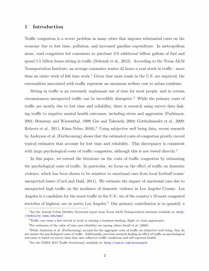
1 Introduction

Traffic congestion is a severe problem in many cities that imposes substantial costs on the

economy due to lost time, pollution, and increased gasoline expenditure. In metropolitan

areas, road congestion led consumers to purchase 2.9 additional billion gallons of fuel and

spend 5.5 billion hours sitting in traffic (Schrank et al., 2012). According to the Texas A&M

Transportation Institute, an average commuter wastes 42 hours a year stuck in traffic - more

than an entire week of full time work.1 Given that most roads in the U.S. are unpriced, the

externalities associated with traffic represent an enormous welfare cost to urban residents.

Sitting in traffic is an extremely unpleasant use of time for most people, and in certain

circumstances unexpected traffic can be incredibly disruptive.2 While the primary costs of

traffic are mostly due to lost time and reliability, there is research using survey data link-

ing traffic to negative mental health outcomes, including stress and aggression (Parkinson,

2001; Hennessy and Wiesenthal, 1999; Gee and Takeuchi, 2004; Gottholmseder et al., 2009;

Roberts et al., 2011; Kunn-Nelen, 2016).3 Using subjective well being data, recent research

by Anderson et al. (Forthcoming) shows that the estimated costs of congestion greatly exceed

typical estimates that account for lost time and reliability. This discrepancy is consistent

with large psychological costs of traffic congestion, although this is not tested directly.4

In this paper, we extend the literature on the costs of traffic congestion by estimating

the psychological costs of traffic. In particular, we focus on the effect of traffic on domestic

violence, which has been shown to be sensitive to emotional cues from local football teams’

unexpected losses (Card and Dahl, 2011). We estimate the impact of emotional cues due to

unexpected high traffic on the incidence of domestic violence in Los Angeles County. Los

Angeles is a candidate for the worst traffic in the U.S.; six of the country’s 10 most congested

stretches of highway are in metro Los Angeles.5 Our primary contribution is to quantify a

1See the Annual Urban Mobility Scorecard report from Texas A&M Transportation Institute available at: http:

//mobility.tamu.edu/ums/.2Traffic can cause a late arrival to work or missing a business meeting, flight, or court appearance.3For estimates of the value of time and reliability see among others Small et al. (2005).4While Anderson et al. (Forthcoming) account for the aggregate costs of traffic on subjective well being, they do

not isolate the psychological costs of traffic. Additionally, previous research finding an effect of traffic on psychologicaloutcomes is based on survey data that uses reflective traffic conditions and self reported health.

5See the INRIX 2015 Traffic Scoreboard, available at: http://inrix.com/scorecard/.

2

http://mobility.tamu.edu/ums/

http://mobility.tamu.edu/ums/

http://inrix.com/scorecard/

specific outcome of the emotional costs of traffic congestion using observational data. We

also build on the literature of the economic consequences of emotional cues. Most people

who are stuck in traffic will not be induced to commit crimes, but still bear a psychological

burden from traffic; therefore we consider our estimates a lower bound on the psychological

cost of traffic.

Our empirical analysis combines police incident reports with observations of local traffic

data in Los Angeles from 2011 to 2015. This rich dataset allows us to link traffic with

criminal activity at a fine spatial and temporal dimension. Our empirical strategy relies on

unexpected traffic shocks to estimate the effect of traffic on domestic violence. We find that

extreme traffic (above the 95th percentile) significantly increases the incidence of domestic

violence by approximately 6%. Since our primary outcome of interest, domestic violence,

typically occurs in the home, we are confident that the offender faced the traffic that is typical

of the commute at the location of the crime. We control for static unobserved effects across

space with fixed effects, and time-varying measures of traffic in the most recent week and

month to control for changes in traffic expectations. Our results are consistent with a model

of emotional cues, and are robust to several specifications and falsification tests. There is

no effect of traffic on lagged crime, no effect of evening traffic on morning crimes, and no

effect of traffic on other categories of crime such as property crime and homicides. Increased

domestic violence is concentrated in low-income and high-crime areas. The effects are also

economically important. Using published estimates of the costs of different crimes indicates

that extreme traffic is responsible for approximately $5-10 million in annual damages due to

increased incidence of domestic violence.6

The rest of the paper is organized as follows: Section 2 discusses the related literature;

Section 3 provides a description of the data and present descriptive statistics; Section 4

presents the empirical strategy; Section 5 is devoted to the main results, heterogeneity of the

impacts and a series of robustness checks; and Section 6 concludes with policy implications.

6Direct and indirect cost to assaults are valued at $107,020 in 2008 dollars according to McCollister et al. (2010).While these additional costs are small relative to the cost of lost time and pollution, we consider them to be extremelower bounds. Domestic violence is severely underreported and most drivers who experience acute congestion willnot commit crimes but still suffer some welfare loss due stress.

3

2 Literature review

Our paper is related to the literature on externalities associated with traffic congestion,

emotional cues and determinants of crime. Several papers find a negative impact of traffic on

psychological health, anger and stress. Gee and Takeuchi (2004) is one of the first papers to

establish a link between self-reported traffic stress with perceived physical and psychological

health conditions. Gottholmseder et al. (2009) improve on the statistical methodology and

find a relationship between commuting features, including travel predictability, and self-

reported stress. More recent work by Kunn-Nelen (2016) shows that while self-reported

commuting times have an impact on self-reported health outcomes and doctor visits, there is

little effect of commuting time on objective health outcomes. Both Roberts et al. (2011) and

Kunn-Nelen (2016) find that effect of commuting on health predominantly manifests itself

in women as opposed to men. Research by Anderson et al. (Forthcoming), using subjective

well being data in China, shows that the estimated costs of congestion greatly exceed typical

estimates that account for lost time and reliability. In the psychology literature, traffic is

found to lead to increased anger and aggression (Parkinson, 2001; Hennessy and Wiesenthal,

1999).

We build on this literature in several ways. First, we link observed traffic data with an

observed stress-related outcome. Most of the traffic data in the existing literature relies on

survey data that only captures a self-reported snapshot of traffic conditions. This mutes

most of the time series variation in actual traffic conditions. Our traffic data are built on

a rich panel of hourly data from different roads and directions that enables us to provide a

representative depiction of actual traffic conditions. Similarly, most of the positive health

effects are also based on self reported outcome data. Conversely, our measure of the psycho-

logical costs of traffic data relies on observed crimes from police incident reports. Therefore,

we significantly advance the literature on the psychological costs of traffic congestion.

This article also fits into a broad literature investigating negative externalities to traffic.

The largest traffic externality is likely the value of time and fuel expenditures associated

with congestion. Schrank et al. (2012) estimates these two categories cost U.S. commuters

$121 billion in 2011. However, the economics literature has also quantified several other

4

externalities of traffic. Ossokina and Verweij (2015) exploits a quasi-experiment that reduce

traffic congestion on certain streets in the Netherlands and find that the decrease in traffic

leads to an increase in housing price. Currie and Walker (2011) show that traffic reductions

due to the introduction of electronic toll collection, (E-ZPass) reduce vehicle emissions near

highway toll plazas, which subsequently reduces prematurity and low birth weight among

mothers near a toll plaza. In addition to negatively affecting infant health, by exploiting

quasi-random variation in wind direction Anderson (2015) shows that traffic has a long run

effect of increasing mortality within the elderly population. Quantifying the total economic

cost of traffic congestion is important when deciding how to optimally manage congestion.

For example, Gibson and Carnovale (2015) shows that tolling not only reduces traffic but

also leads to lower levels of air pollution. Another strand of the literature focus on policies

to reduce externalities to traffic such as congestion pricing through dynamic tolling (e.g.

De Borger and Proost (2013); Gross and Brent (2016)).

Our paper is also related to the literature on unexpected emotional cues and their impact

on economic outcomes. The closest paper in this literature is Card and Dahl (2011) who

study the link between family violence and the emotional cues associated with wins and losses

by professional football teams. They use police reports of violent incidents on Sundays during

the professional football season in the United States. They find that upset losses (defeats

when the home team was predicted to win by four or more points) lead to a 10% increase

in the rate of at-home violence by men against their wives and girlfriends and the impact

is larger for important games. While Card and Dahl (2011) establish an important finding,

there are potentially less policy levers to address unexpected football losses compared to

managing traffic congestion. Additionally, there are a limited number of football games

whereas traffic is a daily concern for many urban residents.

There are several related studies on emotional cues and economic outcomes. Eren and

Mocan (2016) find that criminal sentences set by Louisiana judges for juvenile crimes are

harsher following an unexpected loss by the local university’s football team. Duncan et al.

(2016) shows that emotional cues due to Super Bowl exposure is associated with a small,

but precisely estimated, increase in the probability of low birth weight. There is a related

literature documenting the changes in stress and behavior following a dramatic event. For

5

example, the emotions associated with tragic events have been shown to affect birth outcomes

and student performance.7

Our research is also part of a strand of the literature that studies the determinants

of crime. Crime has been shown to be affected by many different factors. For example,

Schneider et al. (2016) find that domestic violence is affected by negative labor market

conditions. Cui and Walsh (2015) find that following a vacant home foreclosure there is

an increase in violent crime and a smaller increase in property crime. Heaton (2012) finds

that legalization of Sunday packaged liquor sales affect crime. Ranson (2014) finds that

weather and climate change affect crime; temperature has a strong positive effect on criminal

behavior, with little evidence of lagged impacts. Herrnstadt and Muehlegger (2015) estimate

the causal effect of pollution on criminal activity in Chicago by comparing crime on opposite

sides of major interstates on days when the wind blows orthogonally to the direction of

the interstate and find that violent crime is 2.2 percent higher on the downwind side. We

document an additional determinant of crime: the stress caused by unexpected high traffic.

3 Data, descriptive statistics and traffic conditions

3.1 Data sources

Data on crime in Los Angeles come from police incident reports from two sources: the Los

Angeles Police Department (LAPD) and the Los Angeles Sheriff Department (LASD). The

LAPD police reports represent all crimes that take place in the City of Los Angeles and

were accessed via the Los Angeles Open Data website.8 The LAPD data are available from

2011 to 2015 and contain information on the date, time, location and type of crime. The

LASD police report data are obtained through Los Angeles County GIS Data Portal, and

contain data for all crimes in the LASD jurisdiction.9 The LASD serves 40 incorporated

cities and all unincorporated areas of Los Angeles County. These two datasets represent the

7For birth outcomes see Eskenazi et al. (2007) following the September 11th terrorist attacks, and Currie andRossin-Slater (2013) following Hurricane Katrina. For student performance, see Beland and Kim (2016) after ashooting in a high school and Imberman et al. (2012) after a hurricane.

8Data are available at https://data.lacity.org/ by searching for “LAPD Crime and Collision Raw Data”.9The LASD data are available from 2005, but we only use 2011-2015 to match with the LAPD

data. The LASD crime data are accessed at: http://egis3.lacounty.gov/dataportal/2012/03/05/

crime-data-la-county-sheriff/.

6

https://data.lacity.org/

http://egis3.lacounty.gov/dataportal/2012/03/05/crime-data-la-county-sheriff/

http://egis3.lacounty.gov/dataportal/2012/03/05/crime-data-la-county-sheriff/

vast majority of crime in Los Angeles County.10 We consider the following crimes: assault,

domestic violence, property crime, homicides and all crimes.

We control for weather in the city that could affect both crime and traffic. We collect

daily data on rain, maximum temperature and wind speed in Los Angeles from the National

Oceanic and Atmospheric Administration’s (NOAA) National Centers for Environmental

Information.11

The traffic data for Los Angeles are obtained from the California Department of Trans-

portation through the Caltrans Performance Measurement System (PeMS).12 We access

annual Station Hour datasets from 2011 to 2015 from the PeMS data clearinghouse for Cali-

fornia District 7, restricting the stations to Los Angeles County. These datasets contain over

22 million observations of hourly speeds from 543 unique stations in Los Angeles County

for the two major interstates in our analysis. We focus on two major roads, I-10 and I-5,

that represent the primary north-south and east-west routes to downtown Los Angeles. We

also gather data on the location of metro stations from Los Angeles Open Data website and

average zip code-level income data from the U.S. Census American Community Survey.13

3.2 Dataset creations & descriptive statistics

To measure the impact of traffic on crime, we assign each zip code to the closest major

highway that connects to the downtown area. We focus on two major roads, I-10 and I-

5, that represent the primary north-south and east-west routes to downtown Los Angeles.

While these are not the only means of transportation in the Los Angeles Metro area they

are likely to be correlated with traffic on other nearby routes of the same direction. Our

main measure of high traffic is when the cumulative travel time is above the 95th percentile

for a given zip code in a given day. This is built by combining traffic from the morning

and evening travel times based on a typical pattern of driving toward downtown in the

morning and away from downtown in the evening. We explore the robustness of our results

10The maps for the LAPD and LASD jurisdiction are available from the Los Angeles Times: http://maps.latimes.com/lapd/ and http://maps.latimes.com/sheriff/.

11Weather data are available at: https://www.ncdc.noaa.gov/cdo-web/datasets.12The data can be accessed via http://pems.dot.ca.gov/. A free account needs to be established.13Data are available at https://data.lacity.org/A-Livable-and-Sustainable-City/

Los-Angeles-County-Metro-Rail-Station-Portal-Locat/s2k2-nqiy.

7

http://maps.latimes.com/lapd/

http://maps.latimes.com/lapd/

http://maps.latimes.com/sheriff/

https://www.ncdc.noaa.gov/cdo-web/datasets

http://pems.dot.ca.gov/

https://data.lacity.org/A-Livable-and-Sustainable-City/Los-Angeles-County-Metro-Rail-Station-Portal-Locat/s2k2-nqiy

https://data.lacity.org/A-Livable-and-Sustainable-City/Los-Angeles-County-Metro-Rail-Station-Portal-Locat/s2k2-nqiy

to alternate measures of traffic such as the maximum daily travel time for a given zip code.

In order to assign each zip code to the nearest road, we calculate the driving distance from

the zip code centroid to the nearest on-ramp for both I-10 and I-5, two of the major roads

in Los Angeles. This calculation was conducted in ArcGIS using the Network Analyst tool

and the road network for Los Angeles County obtained from the Los Angeles County GIS

Data Portal. Once we have driving distances from each zip code to both I-10 and I-5, we

assign the closest road to the zip code. Since some zip codes are roughly equidistant to I-10

and I-5, as a robustness check we relax the closest route assumption by dropping zip codes

whose difference in driving distances between the two routes are small. Figure 1 presents

the mapping of zip codes to roads. We use a static measure of driving distance to assign a

zip code a time series of traffic from either I-10 or I-5.

Figure 2 presents the traffic congestion by route, direction and time of day. It shows that

the I-10 West is heavy in the morning (between 6:00 and 9:00) with travel time reaching

70 minutes and I-10 East is congested in the afternoon with travel time reaching about 80

minutes (between 15:00 and 18:00). The I-5 North and I-5 South are congested both in the

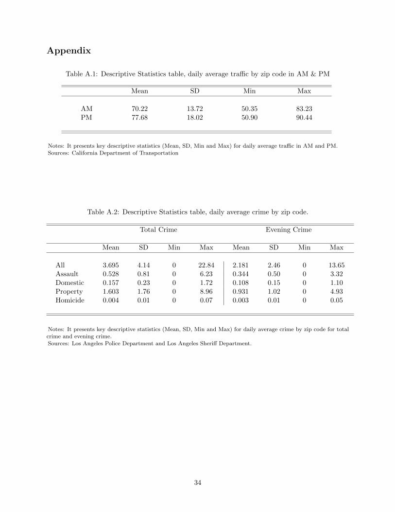
morning and in the afternoon. Table A.1 presents key descriptive statistics (mean, standard

deviation, minimun and maximum) for daily average traffic in AM and PM for zip codes in

our data set. It shows a mean travel time of 70 minutes in the morning and 77 minutes in

the evening. To proxy for the daily commute, we aggregate the typical daily morning and

evening commutes based on the location of the zip code relative to downtown. For example,

a zip code east of downtown will be assigned to I-10 and the cumulative traffic will be the

aggregation of the westbound morning traffic and the eastbound evening traffic.14 We also

analyze the effects of morning and evening traffic separately. The final traffic dataset is a

panel of daily traffic observations for each zip code.

The crime data provide a fine spatial and temporal resolution, and in order to match

the crime data to the traffic data, we aggregate all crimes within a zip code over the course

of the day in each of the categories to obtain our dependent variables.15 All crimes that

14The morning period is defined as 6:00-9:00 AM and the evening period is defined as 3:00-7:00 PM.15The crime data are available at finer spatial resolutions than zip codes, but when aggregating up subcategories,

such as domestic violence, there is little daily variation in the crime data due to a mass of zeros.

8

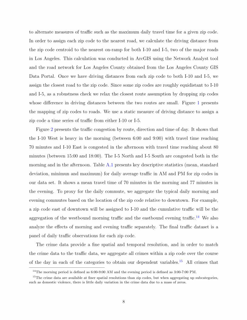
occur before 5 AM are assigned to the previous day and are coded as nighttime crimes. This

allows crimes committed prior to 5 AM to be affected by traffic in the previous day. For

example, we assume that a crime committed at 1:00 AM can be influenced by getting stuck

in traffic on the way home from work. Figure 3 presents a map of average daily domestic

violence incident by zip code in Los Angeles. The maximum daily average domestic violence

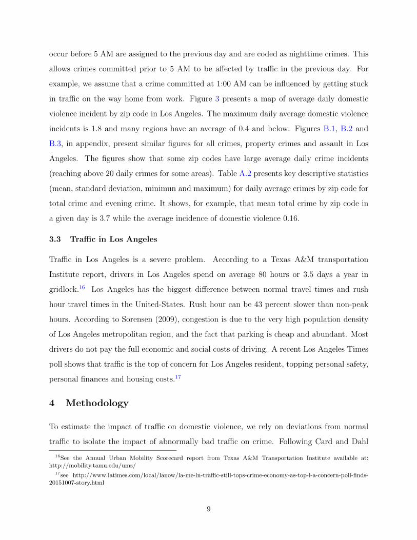
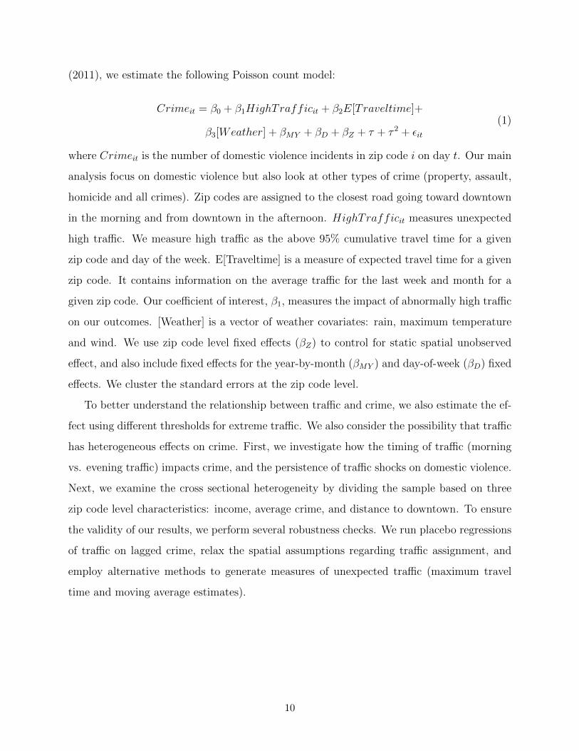
incidents is 1.8 and many regions have an average of 0.4 and below. Figures B.1, B.2 and

B.3, in appendix, present similar figures for all crimes, property crimes and assault in Los

Angeles. The figures show that some zip codes have large average daily crime incidents

(reaching above 20 daily crimes for some areas). Table A.2 presents key descriptive statistics

(mean, standard deviation, minimun and maximum) for daily average crimes by zip code for

total crime and evening crime. It shows, for example, that mean total crime by zip code in

a given day is 3.7 while the average incidence of domestic violence 0.16.

3.3 Traffic in Los Angeles

Traffic in Los Angeles is a severe problem. According to a Texas A&M transportation

Institute report, drivers in Los Angeles spend on average 80 hours or 3.5 days a year in

gridlock.16 Los Angeles has the biggest difference between normal travel times and rush

hour travel times in the United-States. Rush hour can be 43 percent slower than non-peak

hours. According to Sorensen (2009), congestion is due to the very high population density

of Los Angeles metropolitan region, and the fact that parking is cheap and abundant. Most

drivers do not pay the full economic and social costs of driving. A recent Los Angeles Times

poll shows that traffic is the top of concern for Los Angeles resident, topping personal safety,

personal finances and housing costs.17

4 Methodology

To estimate the impact of traffic on domestic violence, we rely on deviations from normal

traffic to isolate the impact of abnormally bad traffic on crime. Following Card and Dahl

16See the Annual Urban Mobility Scorecard report from Texas A&M Transportation Institute available at:http://mobility.tamu.edu/ums/

17see http://www.latimes.com/local/lanow/la-me-ln-traffic-still-tops-crime-economy-as-top-l-a-concern-poll-finds-20151007-story.html

9

(2011), we estimate the following Poisson count model:

Crimeit = β0 + β1HighTrafficit + β2E[Traveltime]+

β3[Weather] + βMY + βD + βZ + τ + τ 2 + εit(1)

where Crimeit is the number of domestic violence incidents in zip code i on day t. Our main

analysis focus on domestic violence but also look at other types of crime (property, assault,

homicide and all crimes). Zip codes are assigned to the closest road going toward downtown

in the morning and from downtown in the afternoon. HighTrafficit measures unexpected

high traffic. We measure high traffic as the above 95% cumulative travel time for a given

zip code and day of the week. E[Traveltime] is a measure of expected travel time for a given

zip code. It contains information on the average traffic for the last week and month for a

given zip code. Our coefficient of interest, β1, measures the impact of abnormally high traffic

on our outcomes. [Weather] is a vector of weather covariates: rain, maximum temperature

and wind. We use zip code level fixed effects (βZ) to control for static spatial unobserved

effect, and also include fixed effects for the year-by-month (βMY ) and day-of-week (βD) fixed

effects. We cluster the standard errors at the zip code level.

To better understand the relationship between traffic and crime, we also estimate the ef-

fect using different thresholds for extreme traffic. We also consider the possibility that traffic

has heterogeneous effects on crime. First, we investigate how the timing of traffic (morning

vs. evening traffic) impacts crime, and the persistence of traffic shocks on domestic violence.

Next, we examine the cross sectional heterogeneity by dividing the sample based on three

zip code level characteristics: income, average crime, and distance to downtown. To ensure

the validity of our results, we perform several robustness checks. We run placebo regressions

of traffic on lagged crime, relax the spatial assumptions regarding traffic assignment, and

employ alternative methods to generate measures of unexpected traffic (maximum travel

time and moving average estimates).

10

5 Results

5.1 Main Results

Table 1 presents the impact of high traffic (above 95th percentile) on domestic violence.

Column (1) uses all traffic and crime observations in Los Angeles to estimate equation

(1), and shows that domestic violence is significantly higher when traffic exceeds the 95th

percentile. Given that we are using a Poisson model the coefficients can be interpreted as the

approximate percentage change in crime once traffic exceeds the 95th percentile. Columns (2)

- (4) focus on subsamples that should be more affected by traffic. Column (2) investigates the

impact of high traffic on domestic violence, excluding the downtown area. We exclude crimes

that occurs downtown since either these crimes are not affected by the typical commuting

pattern, or we cannot be sure which roads the offender traveled to reach downtown. Column

(3) excludes weekends and holidays, since the conventional commuting patterns do not hold

and traffic is inherently less predictable. Column (4) excludes downtown, weekends and

holidays. All specifications show that there is significantly more domestic violence when

there is unexpectedly high traffic. The effects are larger when restricting the sample to those

areas and time periods that represent conventional commuting behavior. Our preferred

specification is column (4), which we use for the remainder of the paper. All subsequent

regressions also include zip code, year-month and day-of-week fixed effects, as well as weather

and recent traffic controls.

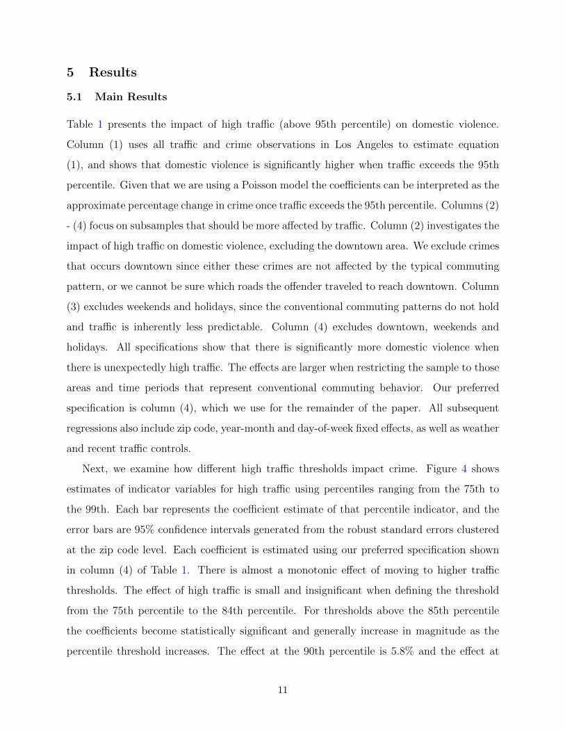
Next, we examine how different high traffic thresholds impact crime. Figure 4 shows

estimates of indicator variables for high traffic using percentiles ranging from the 75th to

the 99th. Each bar represents the coefficient estimate of that percentile indicator, and the

error bars are 95% confidence intervals generated from the robust standard errors clustered

at the zip code level. Each coefficient is estimated using our preferred specification shown

in column (4) of Table 1. There is almost a monotonic effect of moving to higher traffic

thresholds. The effect of high traffic is small and insignificant when defining the threshold

from the 75th percentile to the 84th percentile. For thresholds above the 85th percentile

the coefficients become statistically significant and generally increase in magnitude as the

percentile threshold increases. The effect at the 90th percentile is 5.8% and the effect at

11

the 98th percentile is 9.2%.18 This is consistent with threshold effects, where only traffic in

the right tail can be considered to be unexpected and cause the necessary stress to induce

domestic violence. The damages of traffic can also experience thresholds effects. For example,

drivers may account for certain levels of traffic when commuting, but extreme traffic will

cause them to be late to work and miss important appointments.

Table 2 estimates the effect of traffic on different types of crimes. Column (1) replicates

our preferred specification using domestic violence as the outcome variable. In column (2),

we regress all crimes on traffic, and find that extreme traffic leads to a 1.3% increase in any

type of crime. Column (3) - (5) present results using assaults, property crimes, and homicides

as the outcome variables. Since domestic violence is categorized as an assault we remove

domestic violence incidents from the assault category. There are no significant effects for

assaults, property crime, or homicides.19 The results show that traffic predominantly effects

domestic violence as opposed to other crimes, which is consistent with a model of emotional

cues where unexpected traffic shocks increase psychological stress. It is unlikely that the

psychological stress from traffic would cause an increase in robberies or homicides.

5.2 Heterogeneity

Next, we examine heterogeneous impacts by the timing of unexpected traffic. In particular,

we examine the effect of both morning (AM) and evening (PM) traffic shocks on crime in

addition to each effect separately. Column (2) of Table 3 shows that both the morning and

evening effects are similar in magnitude and significance, which is also corroborated when

examining each effect in isolation (columns (3) and (4)). The effects of PM traffic on crime

are slightly larger but not statistically different from the effects of AM traffic. Column (5)

estimates the effect of traffic that exceeded the 95th percentile in both the morning and the

evening. The effect increases from roughly 6% to over 8%, but the effects are not statistically

different from each other. Lastly, as a placebo test we estimate the effect of traffic in the

18An exception is traffic above the 99th percentile, which is smaller with a very large confidence interval. Theseextreme events are very rare and noisy, and may be due to something other than conventional traffic jams. As arobustness check we replicate Figure 4 when removing all observations above the 99th percentile of traffic. Theresults, presented in Figure B.4 are quantitatively and qualitatively similar.

19The coefficient of the effect on homicides is reasonably large, but is very noisy, because homicides are very rareevents.

12

evening on domestic violence that occurs in the morning (column (6)). Reassuringly, we find

no effect of traffic later in the day on crime in morning.

Table A.3 investigates if the emotional cues due to unexpected high traffic leads to an

increase in domestic violence incidents in the following days. Column (1) of Table A.3

presents results at time T and replicates our preferred specification of Table 1. Columns (2),

(3), and (4) present results at time T + 1, T + 2 and T + 3. The results indicate that the

negative impact of high traffic carries on the following day (T+1) but not after that (not

for T+2 and T+3). Column (5) uses domestic violence incidents at time T or T + 1, as

an outcome variable, showing the cumulative impact of unexpected high traffic on domestic

violence. Including crimes that occur the day after an extreme traffic event increases the

effect size slightly to over 7%.

Next, we examine heterogeneity in the effect of traffic on crime by dividing zip codes

along three dimensions: crime, income and distance to downtown. In each specification we

subset zip codes in the sample by being either above or below the sample median for each

variable.20 Crime and income are correlated, but there are zip codes that are high crime and

high income. Table 4 shows that traffic increases domestic violence in predominantly high-

crime and low-income zip codes. We also find that most of the effect appears to come from

zip codes that are closer to downtown, which may arise for two reasons. First, households

living closer to downtown are more likely to work downtown, and therefore we are assigning

them the appropriate traffic conditions. Secondly, a traffic shock for a household with a very

long commute may be a smaller proportion of their total commute and a traffic shock might

be more expected.

In order to assess the policy levers available to mitigate the effect of traffic on domestic

violence, we examine how access to public transportation affects our results. Table 5 studies

how the proximity to a metro station moderates the effect of traffic on domestic violence.

Table 5 presents results for our measure of unexpected traffic (above the 95th percentile)

but limits the sample to zip codes near a metro station. Columns (1) - (4) of Table 5 limit

the sample to zip codes within 0.5 mile - 3 miles from a metro station. Table 5 shows

20The median fraction of low income households is 68%, the zip code median crime rate is 2 crimes per day, andthe median commute distance is 10.9 miles.

13

once again than unexpected high traffic leads to an increase in domestic violence incident,

and that the negative impact of unexpected high traffic is not reduced by access to public

transportation.21

5.3 Robustness

We perform several robustness checks to test the validity of the results. Our first exercise is

a placebo test where we regress traffic information at time T and crime information in the

previous days: at times T − 1, T − 2, T − 3, and T − 4. High traffic at time T should not

affect crime in previous periods. Table 6 shows that high traffic at time T has no significant

impact on domestic violence incidents in previous days. This is reassuring as high traffic at

time T leads to higher incidence of domestic violence at time T but no increase is observed

in the days prior to the unexpected high traffic.

Our next set of robustness checks relax the assumptions that allow us to match zip codes

to traffic conditions. Columns (1) - (5) of Table 7 restrict the sample to zip codes that are

within one to five miles to the closest on-ramp. Households in these zip codes are more likely

to use the roads that we assign to them. Once again we find that unexpected high traffic leads

to increase in domestic violence incidents. The effects of traffic on domestic violence in these

specifications are larger (7% to 12.1%). These zip codes represent less stringent assumptions

regarding the typical commuting patterns, indicating that our preferred specification may in

fact be a lower bound. We also restrict the sample to zip codes that have a clear choice of

route (I-5 or I-10) by removing zip codes that have similar distances to the two routes. Table

8 replicates our preferred specification for zip codes where the distance between the nearest

on-ramp for I-10 and I-5 is at least 2, 3, 4, and 5 miles. These zip codes are more likely to

be assigned the appropriate traffic conditions. The results do not change substantively; all

the effects are of similar magnitude and statistically significant at the 5% level.

Table 9 presents different measures of high traffic. In column (1) we replace the metric of

travel time with the maximum daily travel time (by hour of day) instead of the cumulative

travel time. Maximum daily travel time is the maximum travel time for all hours in the

21The effects are actually larger in zip codes close to a metro stations. This result is likely driven by the fact thatthese zip codes are closer to downtown, and Table 4 shows that impact of crime on domestic violence is concentratedin zip codes closer to downtown.

14

morning or evening commute. The effect is smaller in magnitude, but still positive and

statistically significant. Next, we model traffic expectations with a variety of moving average

models. In our preferred specification we define unexpected traffic as traffic above the 95th

percentile for each zip code while controlling for recent traffic. The moving average models

use recent traffic to generate a predicted travel time and then examine the deviations from

the prediction as unexpected traffic. In particular, a deviation above the 95th percentile of

all deviations is defined as unexpected extreme traffic. We use three specifications of moving

averages, presented in Table 9. Column (2) uses deviation above the 95% percentile from

the moving average based on the last 5 working days. Column (3) uses a weight of 1/10 for

the last 5 working days and 1/30 for the following 15. Column (4) uses deviations above the

95% percentile from the moving average based on the last 30 working days as a measure of

extreme traffic. All the moving average models produce positive and statistically significant

effects of extreme traffic, indicating that our results are robust to various models of traffic

expectations. Column (5) presents instrumental variable estimates using accidents causing

traffic delays above one hour as our instruments.22 While traffic and accidents are correlated

we believe that the timing and location of severe accidents exploits one specific source of

quasi-random variation in our empirical strategy. Once again, the results indicate that

unexpected high traffic leads to an increase in domestic violence incidents. The coefficient

is slightly larger (+11.45%) and significant at the 10% level.23

Overall, the results are robust to alternative specifications. These numerous robustness

checks and heterogeneity investigation provide confidence that the emotional cues due to

unexpected high traffic leads to high domestic violence incident.

22The accident data is collected from Caltrans.23The correlation between our instrument (accident with long delays) and traffic conditions is 0.22 and the F-test

of the first stage is 12.81.

15

6 Conclusion

This paper investigates the impact of emotional cues due to unexpected high traffic on do-

mestic violence. We combine traffic data in Los Angeles from 2011 to 2015 to police incident

reports from the Los Angeles Police Department and the Los Angeles Sheriff Department.

This rich dataset allows us to link traffic with criminal activity at a fine spatial and temporal

dimension. Our identification relies on extreme deviations from normal traffic to isolate the

impact of abnormally high traffic on domestic violence incidents.

We find that extreme traffic (above the 95th percentile) significantly increases the inci-

dence of domestic violence by approximately 6%. We control for static unobserved effects

across space with fixed effects, and time-varying measures of traffic in the most recent week

and month to control for changes in traffic expectations. We also find that the increase

in domestic violence are concentrated in low-income and high-crime areas. Our results are

consistent with a model of emotional cues, and are robust to several specifications and fal-

sification tests. There is no effect of traffic on lagged crime, no effect of evening traffic on

morning crimes, and no effect of traffic on other categories of crime such as property crime.

The results highlight a new externality associated with traffic in addition to congestion,

pollution, and health impacts that have been established in the literature. This is important

as the direct and indirect costs of a domestic violence incident is estimated to be up to

$107,020 (McCollister et al. (2010)). Our estimates of the economic cost of traffic-induced

domestic violence range from $5-10 million dollars per year depending on the specification.

Since we expect that most people who suffer some psychological costs of traffic do not actually

commit crimes we consider our estimates to be an extreme lower bound; they are the tip

of the iceberg. Documenting the psychological costs of traffic provides additional support

for congestion management policies that not only reduce average travel times but improve

reliability by reducing the variance of travel times. Building new capacity is unlikely to

reduce congestion in the long-run since the elasticity of travel demand change with respect

to capacity is equal to one (Duranton and Turner, 2011). Alternatively, Peirce et al. (2013)

document that drivers report less stress after time-of-day pricing was implemented on a major

road in Seattle. Therefore, our research documents additional benefits of congestion pricing

16

policies, but more research is needed on how different types of tolling structures improve

travel reliability and driver satisfaction.24 There are also implications for how resources

are deployed after extreme traffic events. More police and/or counseling services should be

available when there is high traffic.

References

Anderson, Michael L, “As the Wind Blows: The Effects of Long-Term Exposure to Air

Pollution on Mortality,” NBER Working Paper Series, 2015, (21578).

, Fangwen Lu, Yiran Zhang, Jun Yang, and Ping Qin, “Superstitions, Street Traffic,

and Subjective Well-Being,” Journal of Public Economics, Forthcoming.

Beland, Louis-Philippe and Dongwoo Kim, “The effect of high school shootings on

schools and student performance,” Educational Evaluation and Policy Analysis, 2016, 38

(1), 113–126.

Borger, Bruno De and Stef Proost, “Traffic externalities in cities: the economics of

speed bumps, low emission zones and city bypasses,” Journal of Urban Economics, 2013,

76, 53–70.

Card, David and Gordon B Dahl, “Family violence and football: The effect of unex-

pected emotional cues on violent behavior,” The Quarterly Journal of Economics, 2011,

126 (1), 103.

Cui, Lin and Randall Walsh, “Foreclosure, vacancy and crime,” Journal of Urban Eco-

nomics, 2015, 87, 72–84.

Currie, Janet and Maya Rossin-Slater, “Weathering the storm: Hurricanes and birth

outcomes,” Journal of Health Economics, 2013, 32 (3), 487–503.

24A technical report by the Washington State Department of Transportation shows that dynamically priced high-occupancy toll lanes reduce peak congestion in a road in metro Seattle (WSDOT, 2012).

17

and Reed Walker, “Traffic Congestion and Infant Health: Evidence from E-ZPass,”

American Economic Journal: Applied Economics, 2011, 3 (1), 65–90.

Duncan, Brian, Hani Mansour, and Daniel I Rees, “It’s Just a Game: The Super

Bowl and Low Birth Weight.,” Journal of Human Ressources, 2016.

Duranton, Gilles and Matthew A Turner, “The Fundamental Law of Road Congestion:

Evidence from US Cities,” American Economic Review, 2011, 101 (6), 2616–2652.

Eren, Ozkan and Naci Mocan, “Emotional Judges and Unlucky Juveniles,” 2016, 22611.

Eskenazi, Brenda, Amy R Marks, Ralph Catalano, Tim Bruckner, and Paolo G

Toniolo, “Low birthweight in New York City and upstate New York following the events

of September 11th,” Human Reproduction, 2007, 22 (11), 3013–3020.

Gee, Gilbert C and David T Takeuchi, “Traffic stress, vehicular burden and well-being:

a multilevel analysis,” Social Science & Medicine, 2004, 59 (2), 405–414.

Gibson, Matthew and Maria Carnovale, “The effects of road pricing on driver behavior

and air pollution,” Journal of Urban Economics, 2015, 89, 62–73.

Gottholmseder, Georg, Klaus Nowotny, Gerald J Pruckner, and Engelbert

Theurl, “Stress perception and commuting,” Health Economics, 2009, 18 (5), 559–576.

Gross, Austin and A. Daniel Brent, “Dynamic Road Pricing and the Value of Time

and Reliability,” LSU Working Papers, 2016.

Heaton, Paul, “Sunday liquor laws and crime,” Journal of Public Economics, 2012, 96 (1),

42–52.

Hennessy, Dwight A and David L Wiesenthal, “Traffic congestion, driver stress, and

driver aggression,” Aggressive Behavior, 1999, 25 (6), 409–423.

Herrnstadt, Evan and Erich Muehlegger, “Air Pollution and Criminal Activity: Evi-

dence from Chicago Microdata,” Technical Report, National Bureau of Economic Research

2015.

18

Imberman, Scott A, Adriana D Kugler, and Bruce I Sacerdote, “Katrina’s chil-

dren: Evidence on the structure of peer effects from hurricane evacuees,” The American

Economic Review, 2012, pp. 2048–2082.

Kunn-Nelen, Annemarie, “Does commuting affect health?,” Health Economics, 2016, 25,

984–1004.

McCollister, Kathryn E, Michael T French, and Hai Fang, “The cost of crime to

society: New crime-specific estimates for policy and program evaluation,” Drug and alcohol

dependence, 2010, 108 (1), 98–109.

Ossokina, Ioulia V and Gerard Verweij, “Urban traffic externalities: Quasi-

experimental evidence from housing prices,” Regional Science and Urban Economics, 2015,

55, 1–13.

Parkinson, Brian, “Anger on and off the road,” British Journal of Psychology, 2001, 92

(3), 507–526.

Peirce, Sean, Sean Puckett, Margaret Petrella, Paul Minnice, and Jane Lappin,

“Effects of Full-Facility Variable Tolling on Traveler Behavior: Evidence from a Panel

Study of the SR-520 Corridor in Seattle, Washington,” Transportation Research Record:

Journal of the Transportation Research Board, 2013, (2345), 74–82.

Ranson, Matthew, “Crime, weather, and climate change,” Journal of Environmental Eco-

nomics and Management, 2014, 67 (3), 274–302.

Roberts, Jennifer, Robert Hodgson, and Paul Dolan, “It’s driving her mad: Gen-

der differences in the effects of commuting on psychological health,” Journal of Health

Economics, 2011, 30 (5), 1064–1076.

Schneider, Daniel, Kristen Harknett, and Sara McLanahan, “Intimate partner vio-

lence in the Great Recession,” Demography, 2016, 53 (2), 471–505.

Schrank, David, Bill Eisele, and Tim Lomax, “TTI’s 2012 urban mobility report,”

Proceedings of the 2012 annual urban mobility report. Texas A&M Transportation Institute,

Texas, USA, 2012.

19

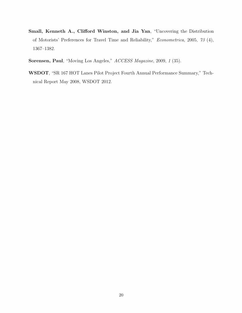
Small, Kenneth A., Clifford Winston, and Jia Yan, “Uncovering the Distribution

of Motorists’ Preferences for Travel Time and Reliability,” Econometrica, 2005, 73 (4),

1367–1382.

Sorensen, Paul, “Moving Los Angeles,” ACCESS Magazine, 2009, 1 (35).

WSDOT, “SR 167 HOT Lanes Pilot Project Fourth Annual Performance Summary,” Tech-

nical Report May 2008, WSDOT 2012.

20

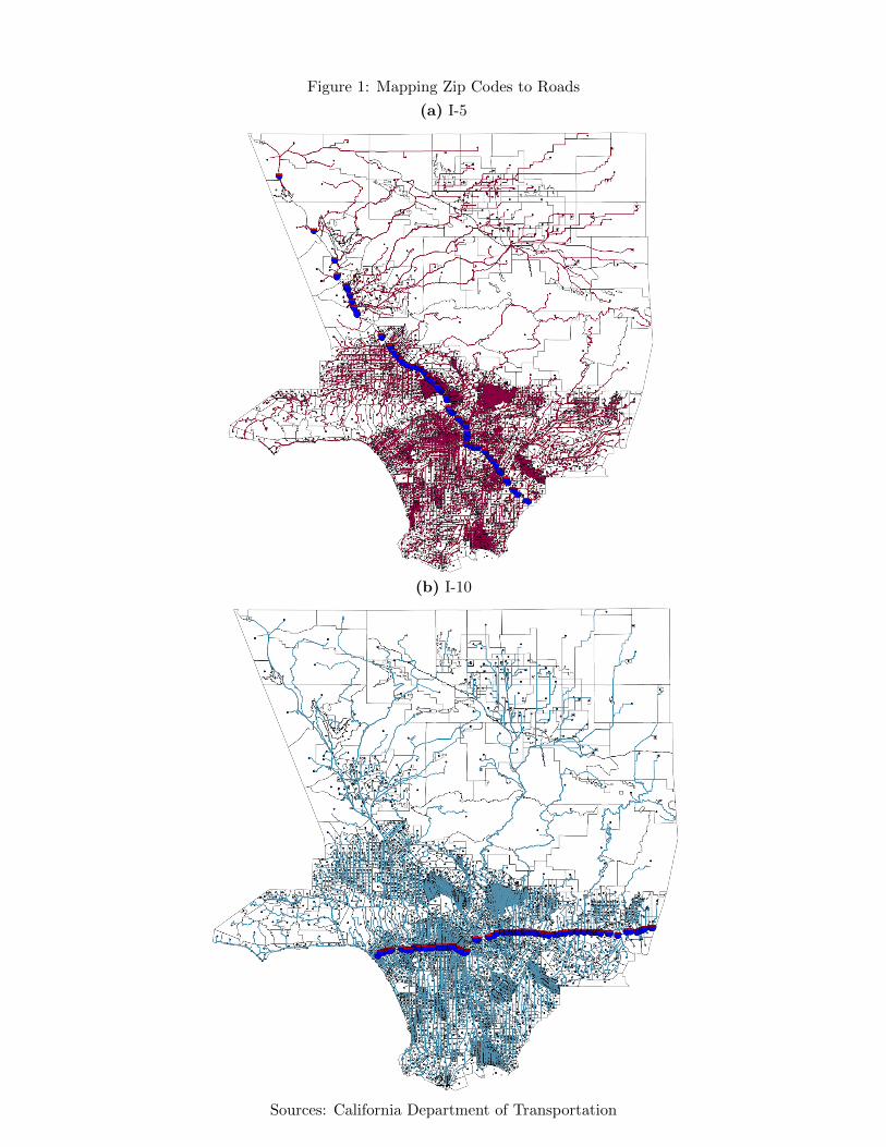
Figure 1: Mapping Zip Codes to Roads

(a) I-5

(b) I-10

Sources: California Department of Transportation

21

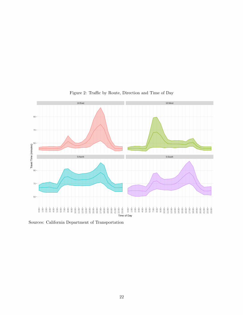
Figure 2: Traffic by Route, Direction and Time of Day

10:East 10:West

5:North 5:South

50

70

90

50

70

90

0:00

1:00

2:00

3:00

4:00

5:00

6:00

7:00

8:00

9:00

10:0

0

11:0

0

12:0

0

13:0

0

14:0

0

15:0

0

16:0

0

17:0

0

18:0

0

19:0

0

20:0

0

21:0

0

22:0

0

23:0

0

0:00

1:00

2:00

3:00

4:00

5:00

6:00

7:00

8:00

9:00

10:0

0

11:0

0

12:0

0

13:0

0

14:0

0

15:0

0

16:0

0

17:0

0

18:0

0

19:0

0

20:0

0

21:0

0

22:0

0

23:0

0

Time of Day

Trav

el T

ime

(min

utes

)

Sources: California Department of Transportation

22

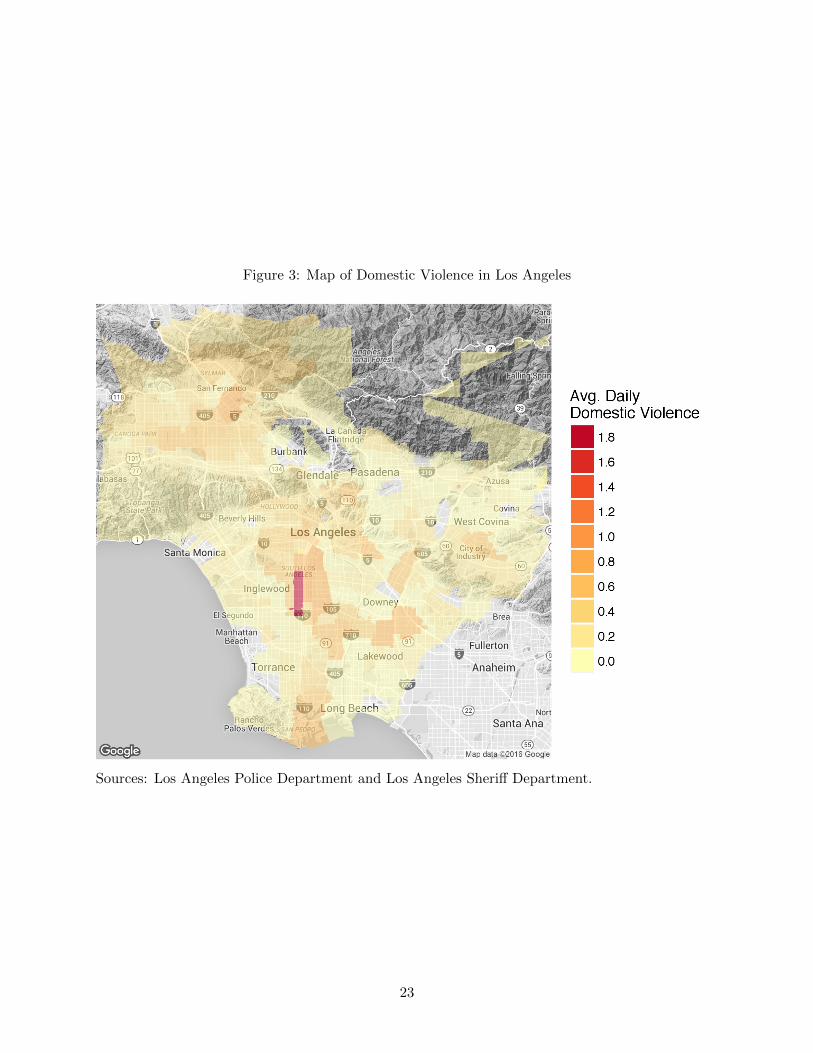
Figure 3: Map of Domestic Violence in Los Angeles

Sources: Los Angeles Police Department and Los Angeles Sheriff Department.

23

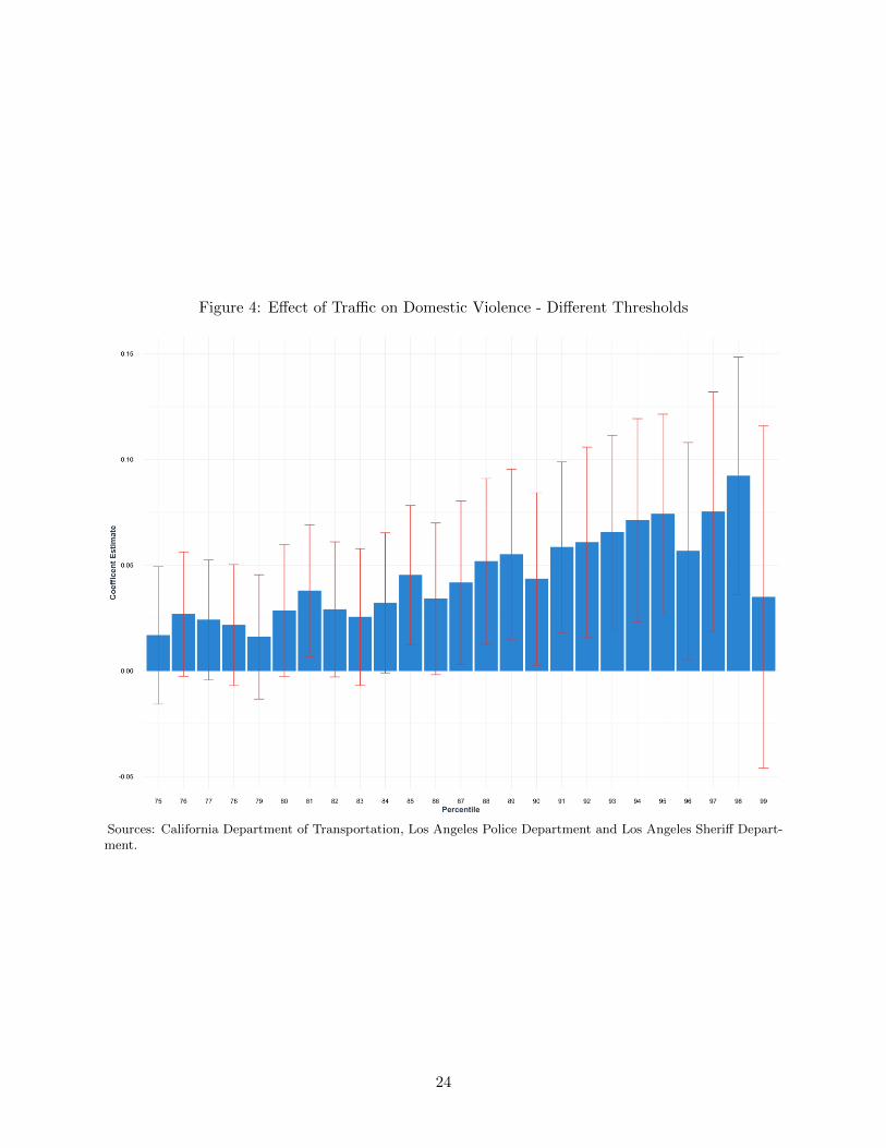
Figure 4: Effect of Traffic on Domestic Violence - Different Thresholds

Sources: California Department of Transportation, Los Angeles Police Department and Los Angeles Sheriff Depart-ment.

24

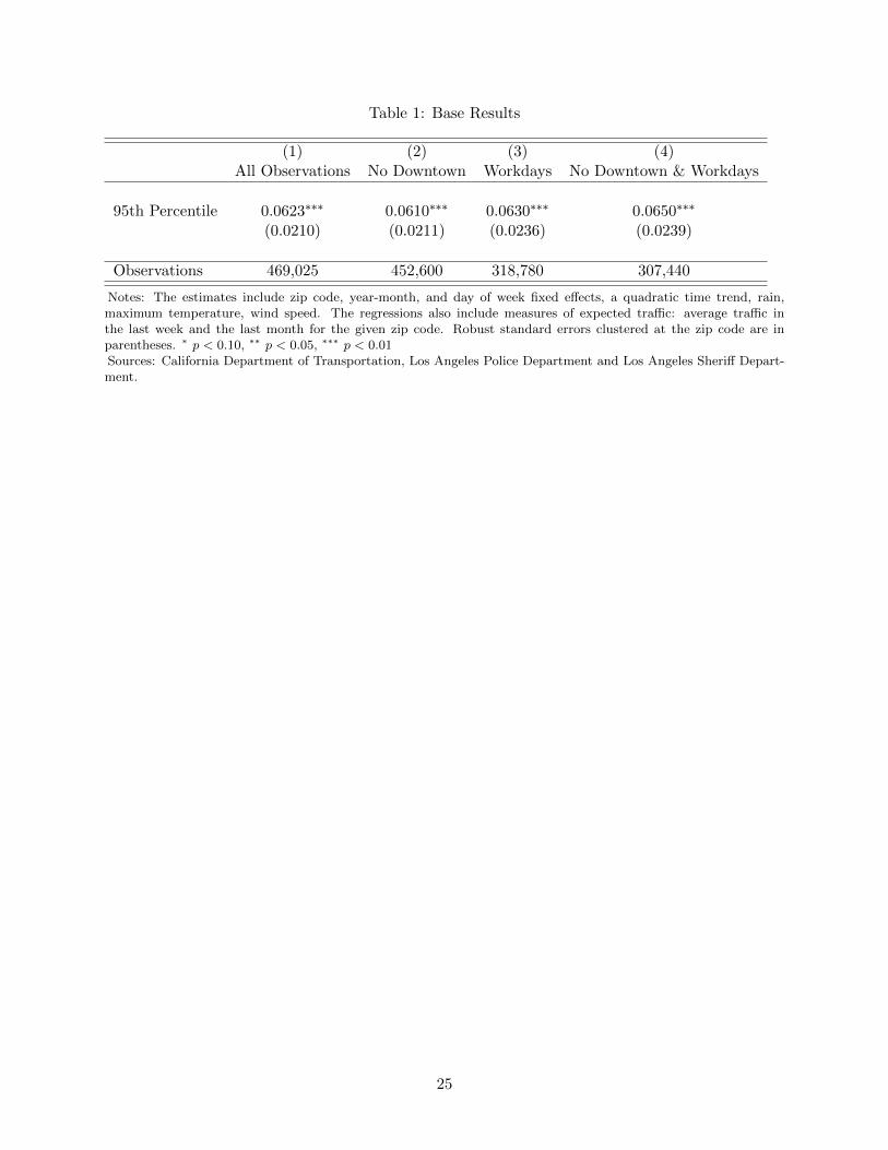
Table 1: Base Results

(1) (2) (3) (4)All Observations No Downtown Workdays No Downtown & Workdays

95th Percentile 0.0623∗∗∗ 0.0610∗∗∗ 0.0630∗∗∗ 0.0650∗∗∗

(0.0210) (0.0211) (0.0236) (0.0239)

Observations 469,025 452,600 318,780 307,440

Notes: The estimates include zip code, year-month, and day of week fixed effects, a quadratic time trend, rain,maximum temperature, wind speed. The regressions also include measures of expected traffic: average traffic inthe last week and the last month for the given zip code. Robust standard errors clustered at the zip code are inparentheses. ∗ p < 0.10, ∗∗ p < 0.05, ∗∗∗ p < 0.01Sources: California Department of Transportation, Los Angeles Police Department and Los Angeles Sheriff Depart-ment.

25

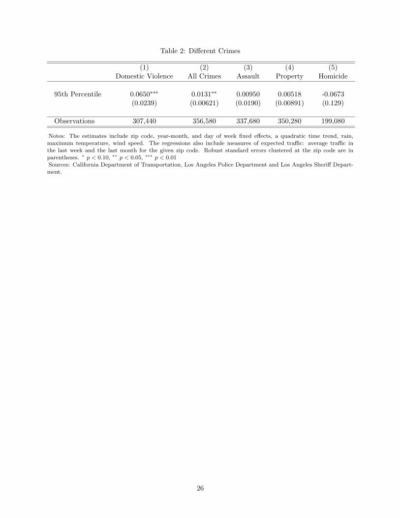
Table 2: Different Crimes

(1) (2) (3) (4) (5)Domestic Violence All Crimes Assault Property Homicide

95th Percentile 0.0650∗∗∗ 0.0131∗∗ 0.00950 0.00518 -0.0673(0.0239) (0.00621) (0.0190) (0.00891) (0.129)

Observations 307,440 356,580 337,680 350,280 199,080


26

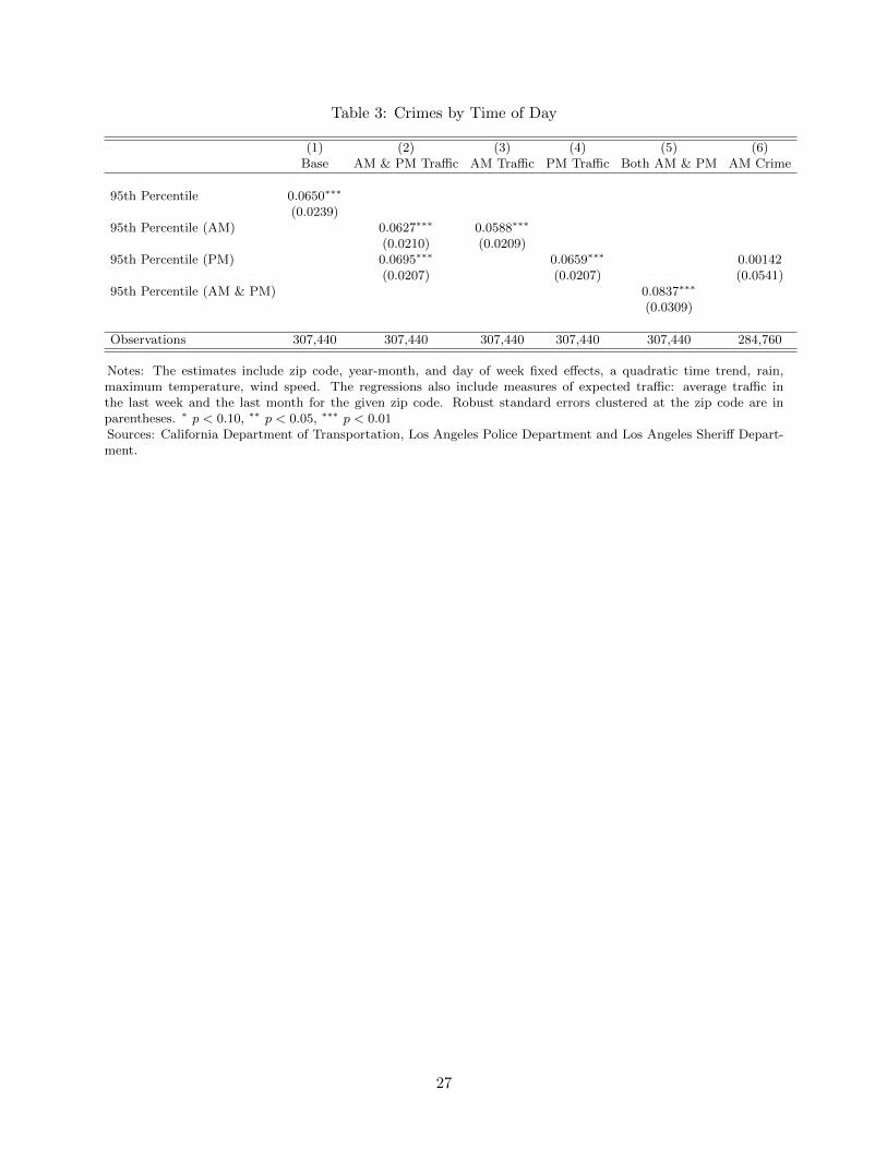
Table 3: Crimes by Time of Day

(1) (2) (3) (4) (5) (6)Base AM & PM Traffic AM Traffic PM Traffic Both AM & PM AM Crime

95th Percentile 0.0650∗∗∗

(0.0239)95th Percentile (AM) 0.0627∗∗∗ 0.0588∗∗∗

(0.0210) (0.0209)95th Percentile (PM) 0.0695∗∗∗ 0.0659∗∗∗ 0.00142

(0.0207) (0.0207) (0.0541)95th Percentile (AM & PM) 0.0837∗∗∗

(0.0309)

Observations 307,440 307,440 307,440 307,440 307,440 284,760


27

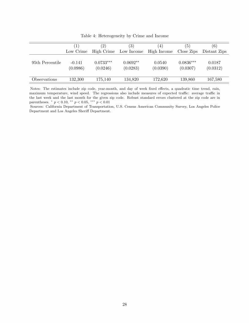
Table 4: Heterogeneity by Crime and Income

(1) (2) (3) (4) (5) (6)Low Crime High Crime Low Income High Income Close Zips Distant Zips

95th Percentile -0.141 0.0733∗∗∗ 0.0692∗∗ 0.0540 0.0836∗∗∗ 0.0187(0.0986) (0.0246) (0.0283) (0.0390) (0.0307) (0.0312)

Observations 132,300 175,140 134,820 172,620 139,860 167,580

Notes: The estimates include zip code, year-month, and day of week fixed effects, a quadratic time trend, rain,maximum temperature, wind speed. The regressions also include measures of expected traffic: average traffic inthe last week and the last month for the given zip code. Robust standard errors clustered at the zip code are inparentheses. ∗ p < 0.10, ∗∗ p < 0.05, ∗∗∗ p < 0.01Sources: California Department of Transportation, U.S. Census American Community Survey, Los Angeles PoliceDepartment and Los Angeles Sheriff Department.

28

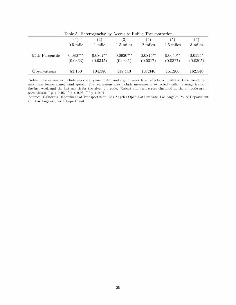
Table 5: Heterogeneity by Access to Public Transportation

(1) (2) (3) (4) (5) (6)0.5 mile 1 mile 1.5 miles 2 miles 2.5 miles 3 miles

95th Percentile 0.0807∗∗ 0.0867∗∗ 0.0920∗∗∗ 0.0815∗∗ 0.0659∗∗ 0.0595∗

(0.0363) (0.0345) (0.0341) (0.0317) (0.0327) (0.0305)

Observations 83,160 104,580 118,440 137,340 151,200 162,540

Notes: The estimates include zip code, year-month, and day of week fixed effects, a quadratic time trend, rain,maximum temperature, wind speed. The regressions also include measures of expected traffic: average traffic inthe last week and the last month for the given zip code. Robust standard errors clustered at the zip code are inparentheses. ∗ p < 0.10, ∗∗ p < 0.05, ∗∗∗ p < 0.01Sources: California Department of Transportation, Los Angeles Open Data website, Los Angeles Police Departmentand Los Angeles Sheriff Department.

29

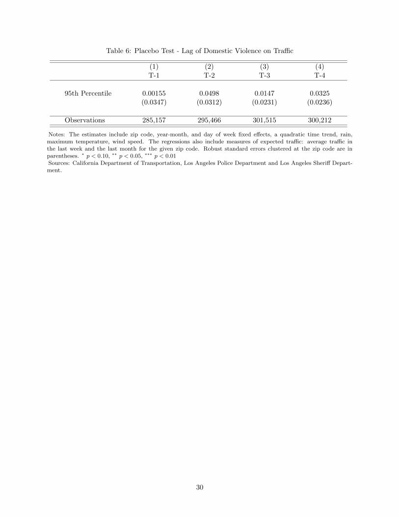
Table 6: Placebo Test - Lag of Domestic Violence on Traffic

(1) (2) (3) (4)T-1 T-2 T-3 T-4

95th Percentile 0.00155 0.0498 0.0147 0.0325(0.0347) (0.0312) (0.0231) (0.0236)

Observations 285,157 295,466 301,515 300,212


30

Table 7: Zip Codes Near On-ramps

(1) (2) (3) (4) (5)1 mile 2 miles 3 miles 4 miles 5 miles

95th Percentile 0.0710 0.0740∗ 0.121∗∗∗ 0.106∗∗∗ 0.0894∗∗∗

(0.0931) (0.0445) (0.0378) (0.0305) (0.0312)

Observations 25,200 55,440 100,800 128,520 154,980


31

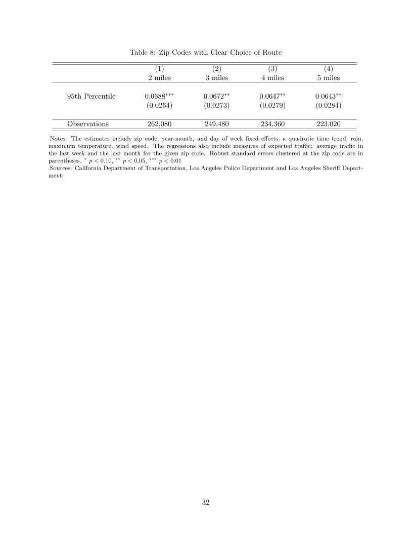
Table 8: Zip Codes with Clear Choice of Route

(1) (2) (3) (4)2 miles 3 miles 4 miles 5 miles

95th Percentile 0.0688∗∗∗ 0.0672∗∗ 0.0647∗∗ 0.0643∗∗

(0.0264) (0.0273) (0.0279) (0.0284)

Observations 262,080 249,480 234,360 223,020


32

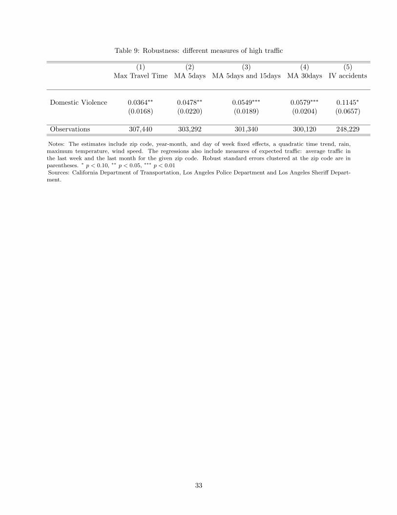
Table 9: Robustness: different measures of high traffic

(1) (2) (3) (4) (5)Max Travel Time MA 5days MA 5days and 15days MA 30days IV accidents

Domestic Violence 0.0364∗∗ 0.0478∗∗ 0.0549∗∗∗ 0.0579∗∗∗ 0.1145∗

(0.0168) (0.0220) (0.0189) (0.0204) (0.0657)

Observations 307,440 303,292 301,340 300,120 248,229


33

Appendix

Table A.1: Descriptive Statistics table, daily average traffic by zip code in AM & PM

Mean SD Min Max

AM 70.22 13.72 50.35 83.23PM 77.68 18.02 50.90 90.44

Notes: It presents key descriptive statistics (Mean, SD, Min and Max) for daily average traffic in AM and PM.Sources: California Department of Transportation

Table A.2: Descriptive Statistics table, daily average crime by zip code.

Total Crime Evening Crime

Mean SD Min Max Mean SD Min Max

All 3.695 4.14 0 22.84 2.181 2.46 0 13.65Assault 0.528 0.81 0 6.23 0.344 0.50 0 3.32Domestic 0.157 0.23 0 1.72 0.108 0.15 0 1.10Property 1.603 1.76 0 8.96 0.931 1.02 0 4.93Homicide 0.004 0.01 0 0.07 0.003 0.01 0 0.05

Notes: It presents key descriptive statistics (Mean, SD, Min and Max) for daily average crime by zip code for totalcrime and evening crime.Sources: Los Angeles Police Department and Los Angeles Sheriff Department.

34

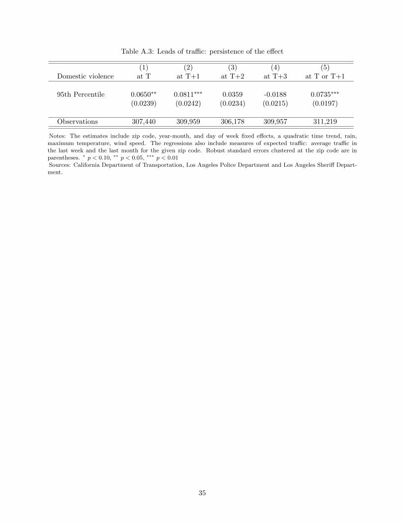
Table A.3: Leads of traffic: persistence of the effect

(1) (2) (3) (4) (5)Domestic violence at T at T+1 at T+2 at T+3 at T or T+1

95th Percentile 0.0650∗∗ 0.0811∗∗∗ 0.0359 -0.0188 0.0735∗∗∗

(0.0239) (0.0242) (0.0234) (0.0215) (0.0197)

Observations 307,440 309,959 306,178 309,957 311,219


35

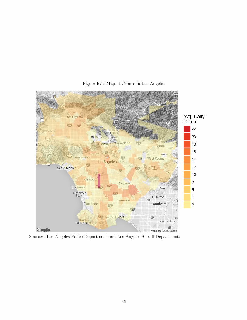
Figure B.1: Map of Crimes in Los Angeles


36

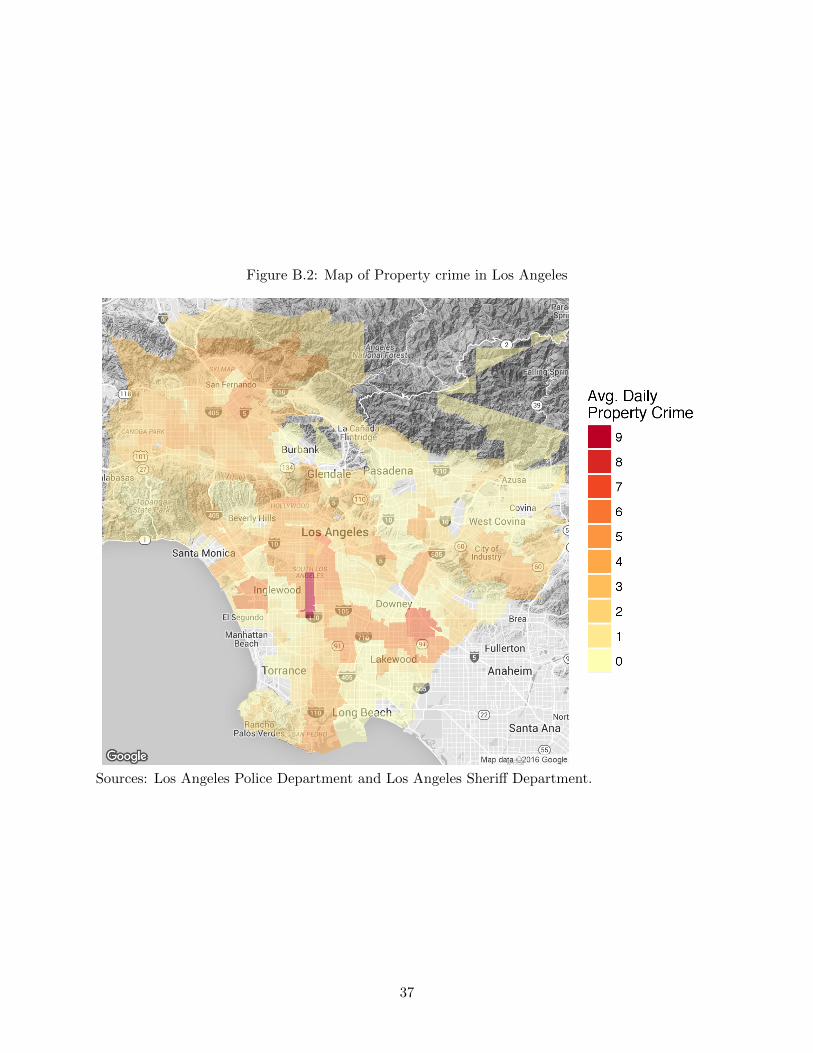
Figure B.2: Map of Property crime in Los Angeles


37

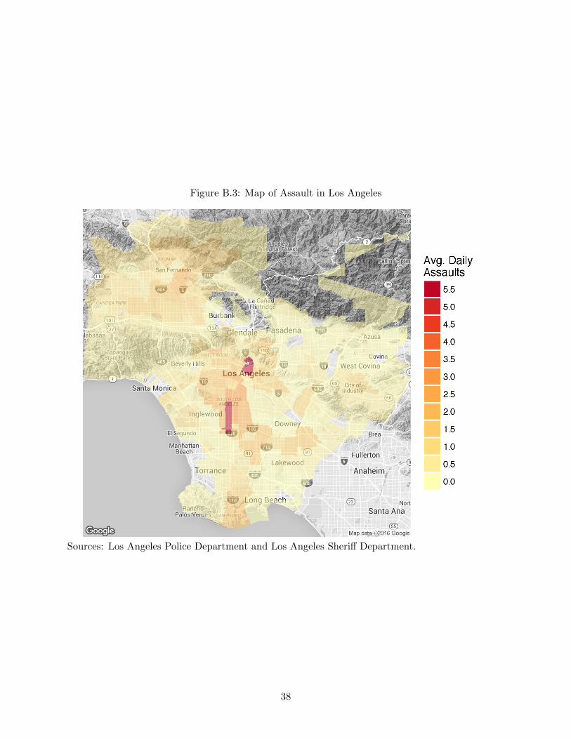
Figure B.3: Map of Assault in Los Angeles


38

Figure B.4: Effect of Traffic on Domestic Violence - Different Thresholds

Sources: California Department of Transportation, Los Angeles Police Department and Los Angeles Sheriff Depart-ment.

39

Documents

Traffic and Crime - Louisiana State Universityfaculty.bus.lsu.edu/papers/pap17_02.pdf · Traffic and Crime Louis-Philippe Beland Louisiana State University Daniel Brent Louisiana