Training a Support Vector Machine in the Primal

Olivier Chapelle

August 30, 2006

Abstract

Most literature on Support Vector Machines (SVMs) concentrate onthe dual optimization problem. In this paper, we would like to point outthat the primal problem can also be solved efficiently, both for linear andnon-linear SVMs, and that there is no reason for ignoring this possibilty.On the contrary, from the primal point of view new families of algorithmsfor large scale SVM training can be investigated.

1 Introduction

The vast majority of text books and articles introducing Support Vector Machines(SVMs) first state the primal optimization problem, and then go directly to thedual formulation [Vapnik, 1998, Burges, 1998, Cristianini and Shawe-Taylor,2000, Scholkopf and Smola, 2002]. A reader could easily obtain the impressionthat this is the only possible way to train an SVM.

In this paper, we would like to reveal this as being a misconception, andshow that someone unaware of duality theory could train an SVM. Primaloptimizations of linear SVMs have already been studied by Keerthi and DeCoste[2005], Mangasarian [2002]. One of the main contributions of this paper is tocomplement those studies to include the non-linear case. 1 Our goal is not toclaim that the primal optimization is better than dual, but merely to show thatthey are two equivalent ways of reaching the same result. Also, we will showthat when the goal is to find an approximate solution, primal optimization issuperior.

Given a training set {(xi, yi)}1≤i≤n,xi ∈ Rd, yi ∈ {+1,−1}, recall that the

primal SVM optimization problem is usually written as:

minw,b||w||2 + C

n∑

i=1

ξpi under constraints yi(w · xi + b) ≥ 1− ξi, ξi ≥ 0. (1)

where p is either 1 (hinge loss) or 2 (quadratic loss). At this point, in theliterature there are usually two main reasons mentioned for solving this problemin the dual:

1Primal optimization of non-linear SVMs have also been proposed in [Lee and Mangasarian,2001b, Section 4], but with a different regularizer.

1

1. The duality theory provides a convenient way to deal with the constraints.

2. The dual optimization problem can be written in terms of dot products,thereby making it possible to use kernel functions.

We will demonstrate in section 3 that those two reasons are not a limitationfor solving the problem in the primal, mainly by writing the optimizationproblem as an unconstrained one and by using the representer theorem. Insection 4, we will see that performing a Newton optimization in the primalyields exactly the same computational complexity as optimizing the dual; thatwill be validated experimentally in section 5. Finally, possible advantages of aprimal optimization are presented in section 6. But we will start now with somegeneral discussion about primal and dual optimization.

2 Links between primal and dual optimization

As mentioned in the introduction, primal and dual optimization have strongconnections and we illustrate some of them through the example of regularizedleast-squares (RLS).

Given a matrix X ∈ Rn×d representing the coordinates of n points in d

dimensions and a target vector y ∈ Rn, the primal RLS problem can be written

asminw∈Rd

λw⊤w + ‖Xw− y‖2, (2)

where λ is the regularization parameter. This objective function is minimizedfor w = (X⊤X + λI)−1X⊤y and its minimum is

y⊤y − y⊤X(X⊤X + λI)−1X⊤y. (3)

Introducing slacks variables ξ = Xw− y, the dual optimization problem is

maxα∈Rn

2α⊤y − 1

λα⊤(XX⊤ + λI)α. (4)

The dual is maximized for α = λ(XX⊤ + λI)−1y and its maximum is

λy⊤(XX⊤ + λI)−1y. (5)

The primal solution is then given by the KKT condition,

w =1

λX⊤α. (6)

Now we relate the inverses of XX⊤+λI and X⊤X +λI thanks to Woodbury

formula [Golub and Loan, 1996, page 51],

λ(XX⊤ + λI)−1 = I −X(λI + X⊤X)−1X⊤ (7)

With this equality, we recover that primal (3) and dual (5) optimal values arethe same, i.e. that the duality gap is zero.

2

0 2 4 6 8 1010

−12

10−10

10−8

10−6

10−4

10−2

100

Number of CG iterations

Prim

al s

ubop

timal

ity

PrimalDual

0 2 4 6 8 1010

−15

10−10

10−5

100

105

Number of CG iterations

Prim

al s

ubop

timal

ity

PrimalDual

Figure 1: Plots of the primal suboptimality, (2)-(3), for primal and dualoptimization by conjugate gradient (pcg in Matlab). n points are drawnrandomly from a spherical Gaussian distribution in d dimensions. The targetsare also randomly generated according a Gaussian distribution. λ is fixed to 1.Left, n = 10 and d = 100. Right, n = 100 and d = 10.

Let us now analyze the computational complexity of primal and dual optimization.The primal requires the computation and inversion of the matrix (X⊤X + λI),which in O(nd2 + d3). On the other hand, the dual deals with the matrix(XX⊤ + λI), which requires O(dn2 + n3) operations to compute and invert. Itis often argued that one should solve either the primal or the dual optimizationproblem depending on whether n is larger or smaller than d, resulting in anO(max(n, d)min(n, d)2) complexity. But this argument does not really holdbecause one can always use (7) in case the matrix to invert is too big. So bothfor primal and dual optimization, the complexity is O(max(n, d)min(n, d)2).

The difference between primal and dual optimization comes when computingapproximate solutions. Let us optimize both the primal (2) and dual (4)objective functions by conjugate gradient and see how the primal objectivefunction decreases as a function of the number of conjugate gradient steps.For the dual optimiztion, an approximate dual solution is converted to anapproximate primal one by using the KKT condition (6).

Intuitively, the primal optimization should be superior because it directlyminimizes the quantity we are interested in. Figure 1 confirms this intuition. Insome cases, there is no difference between primal and dual optimization (left),but in some other cases, the dual optimization can be much slower to converge(right). In Appendix A, we try to analyze this phenomenon by looking at theprimal objective value after one conjugate gradient step. We show that theprimal optimization always yields a lower value than the dual optimization, andwe quantify the difference.

The conclusion from this analyzis is that even though primal and dualoptimization are equivalent, both in terms of the solution and time complexity,when it comes to approximate solution, primal optimization is superior becauseit is more focused on minimizing what we are interested in: the primal objective

3

function.

3 Primal objective function

Coming back to Support Vector Machines, let us rewrite (1) as an unconstrainedoptimization problem:

||w||2 + C

n∑

i=1

L(yi,w · xi + b), (8)

with L(y, t) = max(0, 1 − yt)p (see figure 2). More generally, L could be anyloss function.

−0.5 0 0.5 1 1.50

0.5

1

1.5

2

2.5

3

Output

Loss

LinearQuadratic

Figure 2: SVM loss function, L(y, t) = max(0, 1− yt)p for p = 1 and 2.

Let us now consider non-linear SVMs with a kernel function k and anassociated Reproducing Kernel Hilbert Space H. The optimization problem(8) becomes

minf∈H

λ||f ||2H +n

∑

i=1

L(yi, f(xi)), (9)

where we have made a change of variable by introducing the regularizationparameter λ = 1/C. We have also dropped the offset b for the sake of simplicity.However all the algebra presented below can be extended easily to take it intoaccount (see Appendix B).

Suppose now that the loss function L is differentiable with respect to itssecond argument. Using the reproducing property f(xi) = 〈f, k(xi, ·)〉H, we candifferentiate (9) with respect to f and at the optimal solution f∗, the gradientvanishes, yielding

2λf∗ +n

∑

i=1

∂L

∂t(yi, f

∗(xi))k(xi, ·) = 0, (10)

4

where ∂L/∂t is the partial derivative of L(y, t) with respect to its second argument.This implies that the optimal function can be written as a linear combinationof kernel functions evaluated at the training samples. This result is also knownas the representer theorem [Kimeldorf and Wahba, 1970].

Thus, we seek a solution of the form:

f(x) =n

∑

i=1

βik(xi,x). (11)

We denote those coefficients βi and not αi as in the standard SVM literature tostress that they should not be interpreted as Lagrange multipliers.

Let us express (9) in term of βi,

λn

∑

i,j=1

βiβjk(xi,xj) +n

∑

i=1

L

yi,n

∑

j=1

k(xi,xj)βj

, (12)

where we used the kernel reproducing property in ||f ||2H =∑n

i,j=1 βiβj <

k(xi, ·), k(xj , ·) >H=∑n

i,j=1 βiβjk(xi,xj).

Introducing the kernel matrix K with Kij = k(xi,xj) and Ki the ith columnof K, (12) can be rewritten as

λβ⊤Kβ +n

∑

i=1

L(yi, K⊤i β). (13)

As long as L is differentiable, we can optimize (13) by gradient descent. Notethat this is an unconstrained optimization problem.

4 Newton optimization

The unconstrained objective function (13) can be minimized using a variety ofoptimization techniques such as conjugate gradient. Here we will only considerNewton optimization as the similarities with dual optimization will then appearclearly.

We will focus on two loss functions: the quadratic penalization of the trainingerrors (figure 2) and a differentiable approximation to the linear penalization,the Huber loss.

4.1 Quadratic loss

Let us start with the easiest case, the L2 penalization of the training errors,

L(yi, f(xi)) = max(0, 1− yif(xi))2.

For a given value of the vector β, we say that a point xi is a support vector

if yif(xi) < 1, i.e. if the loss on this point is non zero. Note that this definition

5

of support vector is different from βi 6= 0 2. Let us reorder the training pointssuch that the first nsv points are support vectors. Finally, let I0 be the n × ndiagonal matrix with the first nsv entries being 1 and the others 0,

I0 ≡

1. . . 0

10

0. . .

0

The gradient of (13) with respect to β is

∇ = 2λKβ +

nsv∑

i=1

Ki

∂L

∂t(yi, K

⊤i β)

= 2λKβ + 2

nsv∑

i=1

Kiyi(yiK⊤i β − 1)

= 2(λKβ + KI0(Kβ − Y )), (14)

and the Hessian,H = 2(λK + KI0K). (15)

Each Newton step consists of the following update,

β ← β − γH−1∇,

where γ is the step size found by line search or backtracking [Boyd and Vandenberghe,2004, Section 9.5]. In our experiments, we noticed that the default value of γ = 1did not result in any convergence problem, and in the rest of this section weonly consider this value. However, to enjoy the theorical properties concerningthe convergence of this algorithm, backtracking is necessary.

Combining (14) and (15) as∇ = Hβ−2KI0Y , we find that after the update,

β = (λK + KI0K)−1KI0Y

= (λIn + I0K)−1I0Y (16)

Note that we have assumed that K (and thus the Hessian) is invertible. If Kis not invertible, then the expansion is not unique (even though the solutionis), and (16) will produce one of the possible expansions of the solution. Toavoid these problems, let us simply assume that an infinitesimally small ridgehas been added to K.

Let Ip denote the identity matrix of size p× p and Ksv the first nsv columnsand rows of K, i.e. the submatrix corresponding to the support vectors. Using

2From (10), it turns out at the optimal solution that the sets {i, βi 6= 0} and {i, yif(xi) <

1} will be the same. To avoid confusion, we could have defined this latter as the set of error

vectors.

6

the fact that the lower left block λIn + I0K is 0, the invert of this matrix canbe easily computed, and finally, the update (16) turns out to be

β =

(

(λInsv+ Ksv)

−1 00 0

)

Y,

=

(

(λInsv+ Ksv)

−1Ysv

0

)

. (17)

Link with dual optimization Update rule (17) is not surprising if one hasa look at the SVM dual optimization problem:

maxα

n∑

i=1

αi −1

2

n∑

i,j=1

αiαjyiyj(Kij + λδij), under constraints αi ≥ 0.

Consider the optimal solution: the gradient with respect to all αi > 0 (thesupport vectors) must be 0,

1− diag(Ysv)(Ksv + λInsv)diag(Ysv)α = 0,

where diag(Y ) stands for the diagonal matrix with the diagonal being the vectorY . Thus, up to a sign difference, the solutions found by minimizing the primaland maximizing the primal are the same: βi = yiαi.

Complexity analysis Only a couple of iterations are usually necessary toreach the solution (rarely more than 5), and this number seems independentof n. The overall complexity is thus the complexity one Newton step, which isO(nnsv +n3

sv). Indeed, the first term corresponds to finding the support vectors

(i.e. the points for which yif(xi) < 1) and the second term is the cost ofinverting the matrix Ksv + λInsv

. It turns out that this is the same complexityas in standard SVM learning (dual maximization) since those 2 steps are alsonecessary. Of course nsv is not known in advance and this complexity analysisis an a posteriori one. In the worse case, the complexity is O(n3).

It is important to note that in general this time complexity is also a lowerbound (for the exact computation of the SVM solution). Chunking and decompositionmethods, for instance [Joachims, 1999, Osuna et al., 1997], do not help sincethere is fundamentally a linear system of size nsv to be be solved 3. Chunkingis only useful when the Ksv matrix can not fit in memory.

3We considered here that solving a linear system (either in the primal or in the dual) takescubic time. This time complexiy can however be improved.

7

4.2 Huber / hinge loss

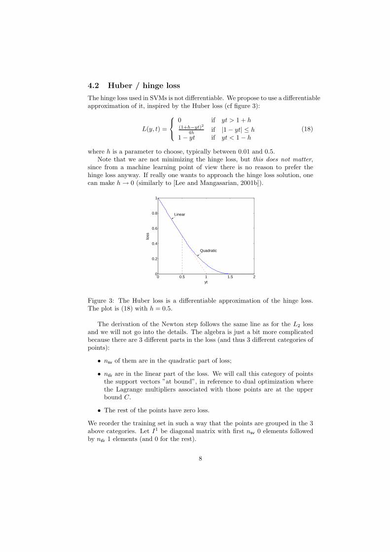
The hinge loss used in SVMs is not differentiable. We propose to use a differentiableapproximation of it, inspired by the Huber loss (cf figure 3):

L(y, t) =

0 if yt > 1 + h(1+h−yt)2

4hif |1− yt| ≤ h

1− yt if yt < 1− h

(18)

where h is a parameter to choose, typically between 0.01 and 0.5.Note that we are not minimizing the hinge loss, but this does not matter,

since from a machine learning point of view there is no reason to prefer thehinge loss anyway. If really one wants to approach the hinge loss solution, onecan make h→ 0 (similarly to [Lee and Mangasarian, 2001b]).

0 0.5 1 1.5 20

0.2

0.4

0.6

0.8

1

yt

loss

Quadratic

Linear

Figure 3: The Huber loss is a differentiable approximation of the hinge loss.The plot is (18) with h = 0.5.

The derivation of the Newton step follows the same line as for the L2 lossand we will not go into the details. The algebra is just a bit more complicatedbecause there are 3 different parts in the loss (and thus 3 different categories ofpoints):

• nsv of them are in the quadratic part of loss;

• nsv are in the linear part of the loss. We will call this category of pointsthe support vectors ”at bound”, in reference to dual optimization wherethe Lagrange multipliers associated with those points are at the upperbound C.

• The rest of the points have zero loss.

We reorder the training set in such a way that the points are grouped in the 3above categories. Let I1 be diagonal matrix with first nsv 0 elements followedby nsv 1 elements (and 0 for the rest).

8

The gradient is

∇ = 2λKβ +KI0(Kβ − (1 + h)Y )

2h−KI1Y

and the Hessian

H = 2λK +KI0K

2h.

Thus,

∇ = Hβ −K

(

1 + h

2hI0 + I1

)

Y

and the new β is

β =

(

2λIn +I0K

2h

)−1 (

1 + h

2hI0 + I1

)

Y

=

(4hλInsv+ Ksv)

−1((1 + h)Ysv −Ksv,svYsv/(2λ))Ysv/(2λ)

0

≡

βsv

βsv

0

.(19)

Again, one can see the link with the dual optimization: letting h → 0, theprimal and the dual solution are the same, βi = yiαi. This is obvious for thepoints in the linear part of the loss (with C = 1/(2λ)). For the points that areright on the margin, their output is equal their label,

Ksvβsv + Ksv,svβsv = Ysv.

But since βsv = Ysv/(2λ),

βsv = K−1sv

(Ysv −Ksv,svYsv/(2λ)),

which is the same equation as the first block of (19) when h→ 0.

Complexity analysis Similar to the quadratic loss, the complexity is O(n3sv

+n(nsv +nsv)). The nsv +nsv factor is the complexity for computing the output ofone training point (number of non zeros elements in the vector β). Again, thecomplexity for dual optimization is the same since both steps (solving a linearsystem of size nsv and computing the outputs of all the points) are required.

4.3 Other losses

Some other losses have been proposed to approximate the SVM hinge loss [Leeand Mangasarian, 2001b, Zhang et al., 2003, Zhu and Hastie, 2005]. However,none of them has a linear part and the overall complexity is O(n3) which canbe much larger than the complexity of standard SVM training. More generally,the size of the linear system to solve is equal to nsv, the number of training

points for which ∂2L∂t2

(yi, f(xi)) 6= 0. If there are some large linear parts in theloss function, this number might be much smaller than n, resulting in significantspeed-up compared to the standard O(n3) cost.

9

5 Experiments

The experiments in this section can be considered as a sanity check to show thatprimal and dual optimization of a non-linear SVM have similar time complexities.However, for linear SVMs, the primal optimization is definitely superior [Keerthiand DeCoste, 2005] as illustrated below.

Some Matlab code for the quadratic penalization of the errors and takinginto account the bias b is available online at: http://www.kyb.tuebingen.mpg.de/bs/people/chapelle/primal.

5.1 Linear SVM

In the case of quadratic penalization of the training errors, the gradient of theobjective function (8) is

∇ = 2w + 2C∑

i∈sv

(w · xi − yi)xi,

and the Hessian isH = Id + C

∑

i∈sv

xix⊤i .

The computation of the Hessian is in O(d2nsv) and its inversion in O(d3).When the number of dimensions is relatively small compared to the number oftraining samples, it is advantageous to optimize directly on w rather than onthe expansion coefficients. In the case where d is large, but the data is sparse,the Hessian should not be built explicitly. Instead, the linear system H−1∇ canbe solved efficiently by conjugate gradient [Keerthi and DeCoste, 2005].

Training time comparison on the Adult dataset [Platt, 1998] in presented infigure 4. As expected, the training time is linear for our primal implementation,but the scaling exponent is 2.2 for the dual implementation of LIBSVM (comparableto the 1.9 reported in [Platt, 1998]). This exponent can be explained as follows: nsv is very small [Platt, 1998, Table 12.3] and nsv grows linearly with n (themisclassified training points). So for this dataset the complexity of O(n3

sv+

n(nsv + nsv)) turns out to be about O(n2).It is noteworthy that, for this experiment, the number of Newton steps

required to reach the exact solution was 7. More generally, this algorithm isusually extremely fast for linear SVMs.

5.2 L2 loss

We now compare primal and dual optimization for non-linear SVMs. To avoidproblems of memory management and kernel caching and to make time comparisonas straightforward as possible, we decided to precompute the entire kernelmatrix. For this reason, the Adult dataset used in the previous section is notsuitable because it would be difficult to fit the kernel matrix in memory (about8G).

10

103

104

10−1

100

101

102

Training set size

Tim

e (s

ec)

LIBSVMNewton Primal

Figure 4: Time comparison of LIBSVM (an implementation of SMO [Platt,1998]) and direct Newton optimization on the normal vector w.

Instead, we used the USPS dataset consisting of 7291 training examples.The problem was made binary by classifying digits 0 to 4 versus 5 to 9. AnRBF kernel with σ = 8 was chosen. We consider in this section the hard marginSVM by fixing λ to a very small value, namely 10−8.

The training for the primal optimization is performed as follows (see Algorithm1): we start from a small number of training samples, train, double the numberof samples, retrain and so on. In this way, the set of support vectors is ratherwell identified (otherwise, we would have to invert an n× n matrix in the firstNewton step).

Algorithm 1 SVM primal training by Newton optimization

Function: β = PrimalSVM(K,Y,λ)n← length(Y) {Number of training points}if n > 1000 then

n2 ← n/2 {Train first on a subset to estimate the decision boundary}β ← PrimalSVM(K1..n2,1..n2

, Y1..n2, λ)]

sv← non zero components of β

else

sv← {1, . . . , n}.end if

repeat

βsv← (Ksv + λInsv

)−1Ysv

Other components of β ← 0sv← indices i such that yi[Kβ]i < 1

until sv has not changed

The time comparison is plotted in figure 5: the running times for primal and

11

dual training are almost the same. Moreover, they are directly proportionalto n3

sv, which turns out to be the dominating term in the O(nnsv + n3

sv) time

complexity. In this problem nsv grows approximatively like√

n. This seems tobe in contradiction with the result of Steinwart [2003], which states than thenumber of support vectors grows linearly with the training set size. Howeverthis result holds only for noisy problems, and the USPS dataset has a very smallnoise level.

102

103

104

10−3

10−2

10−1

100

101

102

Training set size

Tra

inin

g tim

e (s

ec)

LIBSVMNewton − Primaln

sv3 (× 10−8)

Figure 5: With the L2 penalization of the slacks, the parallel between dualoptimization and primal Newton optimization is striking: the training times arealmost the same (and scale in O(n3

sv)). Note that both solutions are exactly the

same.

5.3 Huber loss

We perform the same experiments as in the previous section, but introducednoise in the labels: for randomly chosen 10% of the points, the labels havebeen flipped. In this kind of situation the L2 loss is not well suited, because itpenalizes the noisy examples too much. However if the noise were, for instance,Gaussian in the inputs, then the L2 loss would have been very appropriate.

We will study the time complexity and the test error when we vary theparameter h. Note that the solution will not usually be exactly the same as fora standard hinge loss SVM (it will only be the case in the limit h → 0). Theregularization parameter λ was set to 1/8, which corresponds to the best testperformance.

In the experiments described below, a line search was performed in order tomake Newton converge more quickly. This means that instead of using (19) forupdating β, the following step was made,

β ← β − γH−1∇,

12

where γ ∈ [0, 1] is found by 1D minimization. This additional line search doesnot increase the complexity since it is just O(n). For the L2 loss described inthe previous section, this line search was not necessary and full Newton stepswere taken (γ = 1).

5.3.1 Influence of h

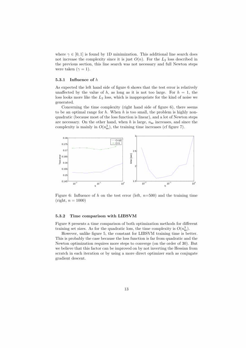
As expected the left hand side of figure 6 shows that the test error is relativelyunaffected by the value of h, as long as it is not too large. For h = 1, theloss looks more like the L2 loss, which is inappropriate for the kind of noise wegenerated.

Concerning the time complexity (right hand side of figure 6), there seemsto be an optimal range for h. When h is too small, the problem is highly non-quadratic (because most of the loss function is linear), and a lot of Newton stepsare necessary. On the other hand, when h is large, nsv increases, and since thecomplexity is mainly in O(n3

sv), the training time increases (cf figure 7).

10−2

10−1

100

0.145

0.15

0.155

0.16

0.165

0.17

0.175

0.18

h

Tes

t err

or

C=10C=1

10−2

10−1

100

1.5

2

2.5

3

h

time

(sec

)

Figure 6: Influence of h on the test error (left, n=500) and the training time(right, n = 1000)

5.3.2 Time comparison with LIBSVM

Figure 8 presents a time comparison of both optimization methods for differenttraining set sizes. As for the quadratic loss, the time complexity is O(n3

sv).

However, unlike figure 5, the constant for LIBSVM training time is better.This is probably the case because the loss function is far from quadratic and theNewton optimization requires more steps to converge (on the order of 30). Butwe believe that this factor can be improved on by not inverting the Hessian fromscratch in each iteration or by using a more direct optimizer such as conjugategradient descent.

13

10−2

10−1

200

250

300

350

400

h

Num

ber

of s

uppo

rt v

ecto

rs

nsv

free

nsv

at bound

Figure 7: When h increases, more points are in the quadratic part of the loss(nsv increases and nsv decreases). The dashed lines are the LIBSVM solution.For this plot, n = 1000.

6 Advantages of primal optimization

As explained throughout this paper, primal and dual optimization are verysimilar, and it is not surprising that they lead to same computational complexity,O(nnsv + n3

sv). So is there a reason to use one rather than the other?

We believe that primal optimization might have advantages for large scale

optimization. Indeed, when the number of training points is large, the numberof support vectors is also typically large and it becomes intractable to computethe exact solution. For this reason, one has to resort to approximations [Bordeset al., 2005, Bakır et al., 2005, Collobert et al., 2002, Tsang et al., 2005]. Butintroducing approximations in the dual may not be wise. There is indeedno guarantee that an approximate dual solution yields a good approximateprimal solution. Since what we are eventually interested in is a good primalobjective function value, it is more straightforward to directly minimize it (cfthe discussion at the end of Section 2).

Below are some examples of approximation strategies for primal minimization.One can probably come up with many more, but our goal is just to give a flavorof what can be done in the primal.

6.1 Conjugate gradient

One could directly minimize (13) by conjugate gradient descent. For squaredloss without regularizer, this approach has been investigated in [Ong, 2005].The hope is that on a lot of problems a reasonable solution can be obtainedwith only a couple of gradient steps.

In the dual, this strategy is hazardous: there is no guarantee that an approximatedual solution corresponds to a reasonable primal solution. We have indeedshown in Section 2 and Appendix A that for a given number of conjugate

14

102

103

104

10−2

10−1

100

101

102

Training set size

Tra

inin

g tim

e (s

ec)

LIBSVM

Newton − primaln

sv3 (× 10−8)

Figure 8: Time comparison between LIBSVM and Newton optimization. Herensv has been computed from LIBSVM (note that the solutions are not exactlythe same). For this plot, h = 2−5.

gradient steps, the primal objective function was lower when optimizing theprimal than when optimizing the dual.

However one needs to keep in mind that the performance of a conjugategradient optimization strongly depends on the parameterization of the problem.In Section 2, we analyzed an optimization in terms of the primal variable w,whereas in the rest of the paper, we used the reparameterization (11) with thevector β. The convergence rate of conjugate gradient depends on the conditionnumber of the Hessian [Shewchuk, 1994]. For an optimization on β, it is roughlyequal to the condition number of K2 (cf equation (15)), while for an optimizationon w, this is the condition number of K.

So optimizing on β could be much slower. There is fortunately an easy fixto this problem: preconditioning by K. In general, preconditioning by a matrixM requires to be able to compute efficiently M−1∇, where ∇ is the gradient[Shewchuk, 1994, Section B5]. But in our case, it turns out that one can factorizeK in the expression of the gradient (14) and the computation of K−1∇ becomestrivial. With this preconditioning (which comes at no extra computational cost),the convergence rate is now the same as for the optimization on w. In fact, inthe case of regularized least squares of section 2, one can show that the conjugategradient steps for the optimization on w and for the optimization on β withpreconditioning are identical.

Pseudocode for optimizing (13) using the Fletcher-Reeves update and thispreconditioning is given in Algorithm 2. Note that in this pseudocode ∇ isexactly the gradient given in (14) but “divided” by K. Finally, we would like topoint out that Algorithm 2 has another interesting interpretation: it is indeedequivalent to performing a conjugate gradients minimization on w (cf (8)),while maintaining the solution in terms of β, i.e. such that w =

∑

βixi. This

15

is possible because at each step of the algorithm, the gradient (with respect tow) is always in the span of the training points. More precisely, we have thatthe gradient of (8) with respect to w is

∑

(∇new)ixi.

Algorithm 2 Optimization of (13) (with the L2 loss) by preconditionedconjugate gradients.

Let β = 0 and d = ∇old = −Yrepeat

Let t∗ be the minimizer of (13) on the line β + td.β ← β + t∗d.Let o = Kβ − Y and sv = {i, oiyi < 1}. Update I0.∇new ← 2λβ + I0o.

d← −∇new +∇⊤

newK∇new

∇⊤

oldK∇old

d.

∇old ← ∇new.until ||∇new || ≤ ε

Let us now have an empirical study of the conjugate gradient behavior. Asin the previous section, we considered the 7291 training examples of the USPSdataset. We monitored the test error as a function of the number of conjugategradient iterations. It can be seen in figure 9 that

• A relatively small number of iterations (between 10 and 100) are enoughto reach a good solution. Note that the test errors at the right of thefigure (corresponding to 128 iterations) are the same as for a fully trainedSVM: the objective values have almost converged at this point.

• The convergence rate depends, via the condition number, on the bandwidthσ. For σ = 1, K is very similar to the identity matrix and one step isenough to be close to the optimal solution. However, the test error is notso good for this value of σ and one should set it to 2 or 4.

It is noteworthy that the preconditioning discussed above is really helpful.For instance, without it, the test error is still 1.84% after 256 iterations withσ = 4.

Finally, note that each conjugate gradient step requires the computation ofKβ (cf equation (14)) which takes O(n2) operations. If one wants to avoidrecomputing the kernel matrix at each step, the memory requirement is alsoO(n2). Both time and memory requirement could probably be improved toO(n2

sv) per conjugate gradient iteration by directly working on the linear system

(19). But this complexity is probably still too high for large scale problems.Here are some cases where the matrix vector multiplication can be done moreefficiently.

Sparse kernel If a compactly supported RBF kernel [Schaback, 1995, Fasshauer,2005] is used, the kernel matrix K is sparse. The time and memory

16

100

101

102

10−2

10−1

Number of CG iterations

Tes

t err

or

σ=1σ=2σ=4σ=8

Figure 9: Optimization of the objective function (13) by conjugate gradient fordifferent values of the kernel width.

complexities are then proportional to the number of non-zeros elements inK. Also, when the bandwidth of the Gaussian RBF kernel is small, thekernel matrix can be well approximated by a sparse matrix.

Low rank Whenever the kernel matrix is (approximately) low rank, one canwrite K ≈ AA⊤ where A ∈ R

n×p can be found through an incompleteCholesky decomposition in O(np2) operations. The complexity of eachconjugate iteration is then O(np). This idea has been used in [Fineand Scheinberg, 2001] in the context of SVM training, but the authorsconsidered only dual optimization. Note that the kernel matrix is usuallylow rank when the bandwidth of the Gaussian RBF kernel is large.

Fast Multipole Methods Generalizing both cases above, Fast Multipole methodsand KD-Trees provide an efficient way of computing the multiplication ofan RBF kernel matrix with a vector [Greengard and Rokhlin, 1987, Grayand Moore, 2000, Yang et al., 2004, de Freitas et al., 2005, Shen et al.,2006]. These methods have been successfully applied to Kernel RidgeRegression and Gaussian Processes, but do not seem to be able to handlehigh dimensional data. See [Lang et al., 2005] for an empirical study oftime and memory requirement of these methods.

6.2 Reduced expansion

Instead of optimizing on a vector β of length n, one can choose a small subset ofthe training points to expand the solution on and optimize only those weights.More precisely, the same objective function (9) is considered, but unlike (11), itis optimized on the subset of the functions expressed as

f(x) =∑

i∈S

βik(xi,x), (20)

17

where S is a subset of the training set. This approach has been pursued in[Keerthi et al., 2006] where the set S is greedily constructed and in [Lee andMangasarian, 2001a] where S is selected randomly. If S contains k elements,these methods have a complexity of O(nk2) and a memory requirement of O(nk).

6.3 Model selection

An other advantage of primal optimization is when some hyperparameters areoptimized on the training cost function [Chapelle et al., 2002, Grandvalet andCanu, 2002]. If θ is a set of hyperparameters and α the dual variables, thestandard way of learning θ is to solve a min max problem (remember that themaximum of the dual is equal to the minimum of the primal):

minθ

maxα

Dual(α, θ),

by alternating between minimization on θ and maximization on α (see forinstance [Grandvalet and Canu, 2002] for the special case of learning scalingfactors). But if the primal is minimized, a joint optimization on β and θ canbe carried out, which is likely to be much faster.

Finally, to compute an approximate leave-one-out error, the matrix Ksv +λInsv

needs to be inverted [Chapelle et al., 2002]; but after a Newton optimization,this inverse is already available in (17).

7 Conclusion

In this paper, we have studied the primal optimization of non-linear SVMs andderived the update rules for a Newton optimization. From these formulae,it appears clear that there are strong similarities between primal and dualoptimization. Also, the corresponding implementation is very simple and doesnot require any optimization libraries.

The historical reasons for which most of the research in the last decade hasbeen about dual optimization are unclear. We believe that it is because SVMswere first introduced in their hard margin formulation [Boser et al., 1992], forwhich a dual optimization (because of the constraints) seems more natural. Ingeneral, however, soft margin SVMs should be preferred, even if the trainingdata are separable: the decision boundary is more robust because more trainingpoints are taken into account [Chapelle et al., 2000].

We do not pretend that primal optimization is better in general; our mainmotivation was to point out that primal and dual are two sides of the same coinand that there is no reason to look always at the same side. And by looking atthe primal side, some new algorithms for finding approximate solutions emergenaturally. We believe that an approximate primal solution is in general superiorto a dual one since an approximate dual solution can yield a primal one whichis arbitrarily bad.

In addition to all the possibilities for approximate solutions metioned inthis paper, the primal optimization also offers the advantage of tuning the

18

hyperparameters simultaneously by performing a conjoint optimization on parametersand hyperparameters.

Acknowledgments

We are grateful to Adam Kowalczyk and Sathiya Keerthi for helpful comments.

A Primal suboptimality

Let us define the following quantities,

A = y⊤y

B = y⊤XX⊤y

C = y⊤XX⊤XX⊤y

After one gradient step with exact line search on the primal objective function,we have w = B

C+λBX⊤y, and the primal value (2) is

1

2A− 1

2

B2

C + λB.

For the dual optimization, after one gradient step, α = λAB+λA

y and by (6),

w = AB+λA

X⊤y. The primal value is then

1

2A +

1

2

(

A

B + λA

)2

(C + λB)− AB

B + λA.

The difference between these two quantities is

1

2

(

A

B + λA

)2

(C + λB)− AB

B + λA+

1

2

B2

C + λB=

1

2

(B2 −AC)2

(B + λA)2(C + λB)≥ 0.

This proves that if ones does only one gradient step, one should do it on theprimal instead of the dual, because one will get a lower primal value this way.

Now note that by the Cauchy-Schwarz inequality B2 ≤ AC, and there isequality only if XX⊤y and y are aligned. In that case the above expression iszero: the primal and dual steps are as efficient. That is what happens on theleft side of Figure 1: when n ≪ d, since X has been generated according toa Gaussian distribution, XX⊤ ≈ dI and the vectors XX⊤y and y are almostaligned.

B Optimization with an offset

We now consider a joint optimization on

(

bβ

)

of the function

f(x) =n

∑

i=1

βik(xi,x) + b.

19

The augmented Hessian (cf (15)) is

2

(

1⊤I01 1⊤I0KKI01 λK + KI0K

)

,

where 1 should be understood as a vector of all 1. This can be decomposed as

2

(

−λ 1⊤

0 K

) (

0 1⊤

I01 λI + I0K

)

.

Now the gradient is

∇ = Hβ − 2

(

1⊤

K

)

I0Y

and the equivalent of the update equation (16) is

(

0 1⊤

I01 λI + I0K

)−1 (

−λ 1⊤

0 K

)−1 (

1⊤

K

)

I0Y =

(

0 1⊤

I01 λI + I0K

)−1 (

0I0Y

)

So instead of solving (17), one solves

(

bβ

sv

)

=

(

0 1⊤

1 λInsv+ Ksv

)−1 (

0Ysv

)

.

References

G. Bakır, L. Bottou, and J. Weston. Breaking SVM complexity with crosstraining. In Proceedings of the 17th Neural Information Processing Systems

Conference, 2005.

A. Bordes, S. Ertekin, J. Weston, and L. Bottou. Fast kernel classifierswith online and active learning. Technical report, NEC Research Institute,Princeton, 2005. http://leon.bottou.com/publications/pdf/huller3.

pdf.

B. Boser, I. Guyon, and V. Vapnik. A training algorithm for optimal marginclassifiers. In Computational Learing Theory, pages 144–152, 1992.

S. Boyd and L. Vandenberghe. Convex Optimization. Cambridge UniversityPress, 2004.

C. Burges. A tutorial on support vector machines for pattern recognition. Data

Mining and Knowledge Discovery, 2(2):121–167, 1998.

O. Chapelle, V. Vapnik, O. Bousquet, and S. Mukherjee. Choosing multipleparameters for support vector machines. Machine Learning, 46:131–159, 2002.

O. Chapelle, J. Weston, L. Bottou, and V. Vapnik. Vicinal risk minimization. InAdvances in Neural Information Processing Systems, volume 12. MIT Press,2000.

20

R. Collobert, S. Bengio, and Y. Bengio. A parallel mixture of svms for verylarge scale problems. Neural Computation, 14(5), 2002.

N. Cristianini and J. Shawe-Taylor. An Introduction to Support Vector

Machines. Cambridge University Press, 2000.

N. de Freitas, Y. Wang, M. Mahdaviani, and D. Lang. Fast krylov methods forn-body learning. In NIPS, 2005.

G. Fasshauer. Meshfree methods. In M. Rieth and W. Schommers, editors,Handbook of Theoretical and Computational Nanotechnology. AmericanScientific Publishers, 2005.

S. Fine and K. Scheinberg. Efficient SVM training using low-rank kernelrepresentations. Journal of Machine Learning Research, 2:243–264, 2001.

G. Golub and Van Loan. Matrix Computations. The Johns Hopkins UniversityPress, Baltimore, 3rd edition, 1996.

Y. Grandvalet and S. Canu. Adaptive scaling for feature selection in svms. InNeural Information Processing Systems, volume 15, 2002.

A. Gray and A. Moore. ’n-body’ problems in statistical learning. In NIPS, 2000.

L. Greengard and V. Rokhlin. A fast algorithm for particle simulations. Journal

of Computational Physics, 73:325–348, 1987.

T. Joachims. Making large-scale SVM learning practical. In Advances in Kernel

Methods - Support Vector Learning. MIT Press, Cambridge, Massachussetts,1999.

S. Keerthi, O. Chapelle, and D. DeCoste. Building support vector machineswith reducing classifier complexity. Journal of Machine Learning Research,7:1493–1515, 2006.

S. S. Keerthi and D. M. DeCoste. A modified finite Newton method for fastsolution of large scale linear svms. Journal of Machine Learning Research, 6:341–361, 2005.

G. S. Kimeldorf and G. Wahba. A correspondence between bayesian estimationon stochastic processes and smoothing by splines. Annals of Mathematical

Statistics, 41:495–502, 1970.

D. Lang, M. Klaas, and N. de Freitas. Empirical testing of fast kernel densityestimation algorithms. Technical Report UBC TR-2005-03, University ofBritish Columbia,, 2005.

Y. J. Lee and O. L. Mangasarian. RSVM: Reduced support vector machines. InProceedings of the SIAM International Conference on Data Mining. SIAM,Philadelphia, 2001a.

21

Y. J. Lee and O. L. Mangasarian. SSVM: A smooth support vector machinefor classification. Computational Optimization and Applications, 20(1):5–22,2001b.

O. L. Mangasarian. A finite Newton method for classification. Optimization

Methods and Software, 17:913–929, 2002.

C. S. Ong. Kernels: Regularization and Optimization. PhD thesis, TheAustralian National University, 2005.

E. Osuna, R. Freund, and F. Girosi. Support vector machines: Trainingand applications. Technical Report AIM-1602, MIT Artificial IntelligenceLaboratory, 1997.

J. Platt. Fast training of support vector machines using sequential minimaloptimization. In Advances in Kernel Methods - Support Vector Learninng.MIT Press, 1998.

R. Schaback. Creating surfaces from scattered data using radial basis functions.In M. Daehlen, T. Lyche, and L. Schumaker, editors, Mathematical Methods

for Curves and Surfaces, pages 477–496. Vanderbilt University Press, 1995.

B. Scholkopf and A. Smola. Learning with kernels. MIT Press, Cambridge, MA,2002.

Y. Shen, A. Ng, and M. Seeger. Fast gaussian process regression using kd-trees.In Advances in Neural Information Processing Systems 18, 2006.

J. R. Shewchuk. An introduction to the conjugate gradient method withoutthe agonizing pain. Technical Report CMU-CS-94-125, School of ComputerScience, Carnegie Mellon University, 1994.

I. Steinwart. Sparseness of support vector machines. Journal of Machine

Learning Research, 4:1071–1105, 2003.

I. W. Tsang, J. T. Kwok, and P. M. Cheung. Core vector machines: fast SVMtraining on very large datasets. Journal of Machine Learning Research, 6:363–392, 2005.

V. Vapnik. Statistical Learning Theory. John Wiley & Sons, 1998.

C. Yang, R. Duraiswami, and L. Davis. Efficient kernel machines using theimproved fast gauss transform. In Advances in Neural Information Processing

Systems 16, 2004.

J. Zhang, R. Jin, Y. Yang, and A. G. Hauptmann. Modified logisticregression: An approximation to svm and its applications in large-scaletext categorization. In Proceedings of the 20th International Conference on

Machine Learning, 2003.

J. Zhu and T. Hastie. Kernel logistic regression and the import vector machine.Journal of Computational and Graphical Statistics, 14:185–205, 2005.

22