Training Deep Neural Networks for Bottleneck Feature ...isl.anthropomatik.kit.edu/cmu-kit/downloads/MA_Jonas_Gehring(1).pdf · Training Deep Neural Networks for Bottleneck Feature

Training Deep Neural Networks forBottleneck Feature Extraction

Master’s Thesis of

Jonas Gehring

Interactive Systems LaboratoriesCarnegie Mellon University, Pittsburgh, USAKarlsruhe Institute of Technology, Germany

Advisor: Prof. Alexander WaibelSecond advisor: Prof. Florian MetzeReviewer: Prof. Alexander WaibelSecond reviewer: Dr. Sebastian Stüker

Duration: June 2012 – December 2012

KIT – University of the State of Baden-Wuerttemberg and National Research Center of the Helmholtz Association www.kit.edu

I declare that I have developed and written the enclosed thesis completely by myself, and

have not used sources or means without declaration in the text.

Karlsruhe, December 7th, 2012

. . . . . . . . . . . . . . . . . . . . . . . . . . . . . . . . . . . . . . . . .

Jonas Gehring

Abstract

In automatic speech recognition systems, preprocessing the audio signal to generate fea-

tures is an important part of achieving a good recognition rate. Previous works have

shown that artificial neural networks can be used to extract good, discriminative features

that yield better recognition performance than manually engineered feature extraction al-

gorithms. One possible approach for this is to train a network with a small bottleneck

layer, and then use the activations of the units in this layer to produce feature vectors for

the remaining parts of the system.

Deep learning is a field of machine learning that deals with e�cient training algorithms

for neural networks with many hidden layers, and with automatic discovery of relevant

features from data. While most frequently used in computer vision, multiple recent works

have demonstrated the ability of deep networks to achieve superior performance on speech

recognition tasks as well.

In this work, a novel approach for extracting bottleneck features from deep neural net-

works is proposed. A stack of denoising auto-encoders is first trained in a layer-wise and

unsupervised manner. Afterwards, the stack is transformed to a feed-forward neural net-

work and a bottleneck layer, an additional hidden layer and the classification layer are

added. The whole network is then fine-tuned to estimate phonetic target states in order

to generate discriminative features in the bottleneck layer.

Multiple experiments on conversational telephone speech in Cantonese show that the pro-

posed architecture can e↵ectively leverage the increased capacity introduced by deep neural

networks by generating more useful features that result in better recognition performance.

Experiments confirm that this ability heavily depends on initializing the stack of auto-

encoders with pre-training. Extracting features from log mel scale filterbank coe�cients

results in additional gains when compared to features from cepstral coe�cients. Further,

small improvements can be achieved by pre-training auto-encoders with more data, which

is an interesting property for settings where only little transcribed data is available.

Evaluations on larger datasets result in significant reductions of recognition error rates (8%

to 10% relative) over baseline systems using standard features, and therefore demonstrate

the general applicability of the proposed architecture.

Acknowledgements

First of all, thanks and kisses go to Kristina and our son Max for their love and amazing

support in all those years, especially during my stay in Pittsburgh. And nothing would

have been possible without our parents, of course.

I like to thank Prof. Alexander Waibel for reaching out to me, providing me with the

opportunity to participate in the interACT exchange program and for constant encourage-

ment. Furthermore, I would like to thank to my supervisor at Carnegie Mellon University,

Prof. Florian Metze, for providing the continuous support that led me through this thesis;

Prof. Ian Lane for GPU computing power in Silicon Valley; Zaid Md Abdul Wahab Sheikh

at CMU for testing many a network during this thesis; Dr. Sebastian Stuker for reviewing

this work; and Denis Stier for proof-reading.

This work was performed at Carnegie Mellon University in Pittsburgh, Pennsylvania dur-

ing the interACT student exchange program and supported by a scholarship from the

Baden-Wurttemberg Stiftung.

This work is supported in part by the Intelligence Advanced Research Projects Activity

(IARPA) via Department of Defense U.S. Army Research Laboratory (DoD/ARL) con-

tract number W911NF-12-C-0015. The U.S. Government is authorized to reproduce and

distribute reprints for Governmental purposes notwithstanding any copyright annotation

thereon. Disclaimer: The views and conclusions contained herein are those of the authors

and should not be interpreted as necessarily representing the o�cial policies or endorse-

ments, either expressed or implied, of IARPA, DoD/ARL, or the U.S. Government.

Contents

1. Introduction 1

1.1. Contribution . . . . . . . . . . . . . . . . . . . . . . . . . . . . . . . . . . . 2

1.2. Layout . . . . . . . . . . . . . . . . . . . . . . . . . . . . . . . . . . . . . . . 2

2. Background 4

2.1. Automatic Speech Recognition . . . . . . . . . . . . . . . . . . . . . . . . . 4

2.1.1. System Overview . . . . . . . . . . . . . . . . . . . . . . . . . . . . . 4

2.1.2. Preprocessing . . . . . . . . . . . . . . . . . . . . . . . . . . . . . . . 5

2.1.3. Acoustic Modeling . . . . . . . . . . . . . . . . . . . . . . . . . . . . 6

2.2. Artificial Neural Networks . . . . . . . . . . . . . . . . . . . . . . . . . . . . 7

2.2.1. Tandem Systems for ASR . . . . . . . . . . . . . . . . . . . . . . . . 8

2.3. Deep Learning . . . . . . . . . . . . . . . . . . . . . . . . . . . . . . . . . . 10

2.3.1. Applications to Acoustic Modeling . . . . . . . . . . . . . . . . . . . 11

2.3.2. Stacked, Denoising Auto-encoders . . . . . . . . . . . . . . . . . . . 12

2.3.2.1. Auto-encoder Neural Networks . . . . . . . . . . . . . . . . 12

2.3.2.2. Adding a Denoising Criterion . . . . . . . . . . . . . . . . . 13

2.3.2.3. Building Deep Neural Networks . . . . . . . . . . . . . . . 15

3. Bottleneck Features from Deep Neural Networks 16

3.1. Previous Work . . . . . . . . . . . . . . . . . . . . . . . . . . . . . . . . . . 16

3.2. Model Description and Training Procedure . . . . . . . . . . . . . . . . . . 17

3.2.1. Denoising Auto-Encoders for Speech . . . . . . . . . . . . . . . . . . 19

3.2.2. Layer-wise Pre-training . . . . . . . . . . . . . . . . . . . . . . . . . 19

3.2.3. Adding the Bottleneck and Fine-tuning . . . . . . . . . . . . . . . . 21

3.3. Usage in an Automatic Speech Recognition System . . . . . . . . . . . . . . 22

3.3.1. Initial Setup and Training Data Generation . . . . . . . . . . . . . . 22

3.3.2. Feature Extraction . . . . . . . . . . . . . . . . . . . . . . . . . . . . 22

4. Experiments 24

4.1. Baseline Systems . . . . . . . . . . . . . . . . . . . . . . . . . . . . . . . . . 24

4.1.1. The Janus Recognition Toolkit . . . . . . . . . . . . . . . . . . . . . 24

ix

x Contents

4.1.2. System Configurations . . . . . . . . . . . . . . . . . . . . . . . . . . 24

4.1.2.1. Development System . . . . . . . . . . . . . . . . . . . . . 24

4.1.2.2. Cantonese . . . . . . . . . . . . . . . . . . . . . . . . . . . 25

4.1.2.3. Tagalog . . . . . . . . . . . . . . . . . . . . . . . . . . . . . 25

4.1.2.4. Switchboard . . . . . . . . . . . . . . . . . . . . . . . . . . 25

4.2. Evaluation Criteria . . . . . . . . . . . . . . . . . . . . . . . . . . . . . . . . 26

4.3. Experiments on the Development System . . . . . . . . . . . . . . . . . . . 26

4.3.1. Input Data . . . . . . . . . . . . . . . . . . . . . . . . . . . . . . . . 26

4.3.2. Training on More Data . . . . . . . . . . . . . . . . . . . . . . . . . 27

4.3.3. Importance of Pre-training . . . . . . . . . . . . . . . . . . . . . . . 28

4.4. Evaluation on Larger Systems . . . . . . . . . . . . . . . . . . . . . . . . . . 31

4.4.1. Cantonese . . . . . . . . . . . . . . . . . . . . . . . . . . . . . . . . . 31

4.4.2. Tagalog . . . . . . . . . . . . . . . . . . . . . . . . . . . . . . . . . . 31

4.4.3. Switchboard . . . . . . . . . . . . . . . . . . . . . . . . . . . . . . . . 32

5. Conclusion 34

5.1. Summary . . . . . . . . . . . . . . . . . . . . . . . . . . . . . . . . . . . . . 34

5.2. Discussion . . . . . . . . . . . . . . . . . . . . . . . . . . . . . . . . . . . . . 35

5.3. Outlook . . . . . . . . . . . . . . . . . . . . . . . . . . . . . . . . . . . . . . 35

Bibliography 37

Appendix 43

A. Training Algorithms . . . . . . . . . . . . . . . . . . . . . . . . . . . . . . . 43

A.1. Denoising Auto-encoder . . . . . . . . . . . . . . . . . . . . . . . . . 43

A.2. Multi-layer Perceptron . . . . . . . . . . . . . . . . . . . . . . . . . . 44

A.3. Stochastic Mini-batch Gradient Descent . . . . . . . . . . . . . . . . 45

B. Neural Network Training on Graphics Processors . . . . . . . . . . . . . . . 46

B.1. Software . . . . . . . . . . . . . . . . . . . . . . . . . . . . . . . . . . 46

B.2. Training Time . . . . . . . . . . . . . . . . . . . . . . . . . . . . . . 46

x

Introduction

During the last decade of research in automatic speech recognition (ASR), the field has

faced an enormous number of applications. The growing amount of computational re-

sources available paves the way for using speech recognition in tasks like real-time trans-

lation, audio analysis of videos or keyword search in large archives of recordings. With

computers and mobile phones becoming increasingly ubiquitous, those systems are gaining

importance as providers of natural and intuitive human-computer interfaces. Generally

speaking, speech is the fundamental medium of communication between humans, and en-

abling machines to handle this medium reasonably well is of major concern to researchers.

But as the number of applications continues to increase, so do the challenges current

systems have to overcome.

While constrained tasks on read speech with limited vocabularies have long been mastered

and have led to many successful applications, progress of conventional systems on more

di�cult problems has been slow over the last decade. Conversational, large-vocabulary

speech continues to be a major issue for current systems. Further challenges are caused

by inherent variations such as background noise, speaker style or age, accents and more

that humans are able to master while machines are still struggling.

Recent works have demonstrated the ability of deep learning techniques to bring the per-

formance of recognizers on challenging tasks to the next level. This field deals with the

training of powerful models called deep neural networks, that are able to e↵ectively handle

the plethora of variations that makes classification of raw data like images and speech so

di�cult. Many algorithms also provide ways to improve performance by leveraging unla-

beled data, which is especially attractive for ASR, where preparing training data is still

very labor-intense. While the challenges mentioned above have not been fully mastered

yet, it has become clear that deep neural networks are going to play an important role in

overcoming them.

Most of the work on the application of deep learning to speech recognition has been

1

2 1. Introduction

done by improving acoustic models that estimate the likelihood of a speech signal given

a corresponding symbolic representation like a phoneme sequence. In current systems,

this task is performed by hidden Markov models that model the human speech production

process. Hybrid systems in which those models are combined with deep neural networks

have therefore become popular.

An alternative approach is using neural networks to generate the input features used by

a conventional system employing a combination of Gaussian mixture models and hidden

Markov models for acoustic modeling. This is done by training a network to classify

phoneme states and then using the network output (probabilistic features) or the activa-

tions of a narrow hidden layer (bottleneck features) to generate the features for the main

system. Applying deep neural networks to this task is appealing, too, because many sys-

tems already include support for generating features this way. Furthermore, the behaviour

of the remaining system in combination with those features is well-understood, which helps

when integrating and comparing di↵erent types of networks.

1.1. Contribution

This thesis describes a novel approach of using deep neural networks for bottleneck feature

extraction as a preprocessing step for acoustic modeling, and demonstrates its superiority

over conventional setups. In particular, it is being shown that the pre-training algorithms

popular in the deep learning community produce better neural network models compared

to standard methods, and that deeper neural networks result in better performance of the

resulting speech recognition system.

The models proposed were evaluated in a state-of-the-art recognition system on challenging

real-world tasks with conversational telephone speech in languages that are new to the

research community. Additional evaluation on a standard benchmark task shows that the

approach presented is generally applicable.

1.2. Layout

The next chapter provides the theoretical background for the main contributions of this

work and introduces the relevant concepts of automatic speech recognition, artificial neural

networks and deep learning. Chapter three discusses previous work on using deep learning

to generate bottleneck features and describes the models, algorithms and training proce-

dures proposed. The fourth chapter documents the experiments done during the course of

this thesis and provides an evaluation of the techniques introduced previously. The ASR

system and the individual setups used will be described as well. The results are then sum-

marized and discussed in chapter five, followed by an outlook suggesting possible future

work.

2

1.2. Layout 3

Detailed mathematical descriptions of the training algorithms used as well as implementa-

tion notes regarding the training of neural networks on graphics processors can be found

in the respective appendices.

3

Background

2.1. Automatic Speech Recognition

The term automatic speech recognition (ASR) describes the process of extracting a textual

representation of spoken words from a sound signal when performed by a machine, e.g. a

computer. Usually, the physical signal caused by a human uttering a sequence of words is

recording using a microphone and converted to a digital representation of a sound wave.

This is the input to the ASR system, which tries to find a sequence of words as close as

possible to the ones originally uttered.

The multiple levels of ambiguity present in human communication make ASR a very

challenging task. Background noise, noisy channels like telephone lines, speaker variability

or conversational (“sloppy”) speech pose additional di�culties that even modern systems

still struggle with. Nonetheless, speech recognition systems are expected to achieve near-

human levels of performance in scenarios like human-machine interfaces.

2.1.1. System Overview

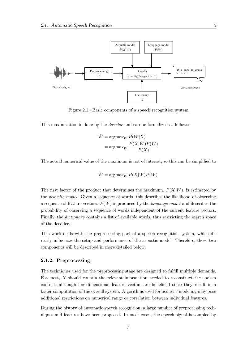
A typical ASR system consists of five major building blocks that are illustrated in Fig-

ure 2.1. During preprocessing, the digitalized sound signal recorded over a period of time

is transformed into a sequence of feature vectors X. The goal of the whole system is to

determine the most likely sequence of words W given a sequence of feature vectors X.

This is equal to maximizing the a posteriori probability P (W |X), which can be expressed

using Bayes’ rule as

P (W |X) =P (X|W )P (W )

P (X)

4

2.1. Automatic Speech Recognition 5

Preprocessing

Acoustic model

P (X|W )

Decoder

Language model

P (W )

X

Dictionary

W

W = argmaxWP (W |X)

Speech signal

It’s hard to wreck

a nice...

Word sequence

Figure 2.1.: Basic components of a speech recognition system

This maximization is done by the decoder and can be formalized as follows:

W = argmaxW P (W |X)

= argmaxWP (X|W )P (W )

P (X)

The actual numerical value of the maximum is not of interest, so this can be simplified to

W = argmaxW P (X|W )P (W )

The first factor of the product that determines the maximum, P (X|W ), is estimated by

the acoustic model. Given a sequence of words, this describes the likelihood of observing

a sequence of feature vectors. P (W ) is produced by the language model and describes the

probability of observing a sequence of words independent of the current feature vectors.

Finally, the dictionary contains a list of available words, thus restricting the search space

of the decoder.

This work deals with the preprocessing part of a speech recognition system, which di-

rectly influences the setup and performance of the acoustic model. Therefore, those two

components will be described in more detailed below.

2.1.2. Preprocessing

The techniques used for the preprocessing stage are designed to fulfill multiple demands.

Foremost, X should contain the relevant information needed to reconstruct the spoken

content, although low-dimensional feature vectors are beneficial since they result in a

faster computation of the overall system. Algorithms used for acoustic modeling may pose

additional restrictions on numerical range or correlation between individual features.

During the history of automatic speech recognition, a large number of preprocessing tech-

niques and features have been proposed. In most cases, the speech signal is sampled by

5

6 2. Background

consecutively computing the response to a short Hamming window, which produces small

time frames that are assumed to be periodic signals for further processing. This makes it

possible to apply a discrete Fourier transform yielding a power spectrum of isolated sound

waves at di↵erent frequencies. Commonly, the powers are mapped to the mel scale, which

approximates the perception of the human ear.

The most popular features used in ASR systems today are mel frequency cepstral coef-

ficients, or MFCCs [DM80]. In order to generate them, the mel coe�cients obtained

using the technique described above are treated as a signal themselves. A discrete cosine

transform is applied to their logarithm, resulting in the individual MFCCs.

Acoustic models usually benefit from increased temporal context per feature vector, so

features extracted from consecutive windowed speech segments are concatenated to form

a feature frame. Finally, a dimensionality reduction technique such as linear discriminant

analysis (LDA) produces the final feature vector that is used by the recognition system.

This thesis deals with using artificial neural networks to generate discriminative features

out of traditional features like mel-scale coe�cients or MFCCs. In combination with the

traditional GMM/HMM approach introduced in the next section, this is usually referred to

as a tandem system [HES00], [GKKC07]. This is described in more detail in section 2.2.1

after neural networks have been introduced.

2.1.3. Acoustic Modeling

As described in section 2.1.1, acoustic models are used to estimate the probability that the

current sequence of feature vectors are being observed given a sequence of words. Given

the multitude of variations regarding speaker style or age, background noises etc. and

combining them with additional variations in time makes this a very challenging problem.

In current systems, acoustic modeling is usually approached using hidden Markov models

(HMMs). HMMs model Markov processes where only the results but not the process

producing them can be observed. In the ASR context, the process corresponds to the

contraction of muscles in the human vocal tract and the result is the sound captured by a

microphone, or feature vectors generated by the preprocessing stage.

The states of the speech production process are commonly modeled as sub-word units such

as multi-state phonemes or senones. Since processes modeled with HMMs are assumed

to fulfill the Markov property, i.e. that the next state of a process depends on its current

state only, each observance is assumed to solely depend on the current state as well. For

speech, this means that sub-word units are modeled independent of their temporal context,

which does not reflect the reality. In order to overcome this limitation, current systems

use context-dependent states, where sub-word units with di↵erent surrounding units are

assigned to di↵erent HMM states.

Performing computations with hidden Markov models requires two probability distribu-

tions: emission probabilities of the possible results that can be observed and transition

6

2.2. Artificial Neural Networks 7

probabilities between the di↵erent states of the process. Training algorithms to estimate

the latter require existing emission probabilities, which have to be learned separately from

the available data. Current systems typically employ Gaussian mixture models (GMMs)

to estimate the probability that a feature vector corresponds to a specific sub-word unit,

that are usually trained using variants of the Expectation-Maximization algorithm.

2.2. Artificial Neural Networks

Artificial neural networks (ANNs) have been of interest to researchers for decades, albeit

with varying degrees thanks to repeated waves of popularity and aversion by the scientific

community. In 1958, Rosenblatt first introduced perceptrons, simple computational units

crudely modelled after biological neurons, and a corresponding training procedure for

using them as linear classifiers [Ros58]. Decades later, Rumelhardt et al. proposed the

backpropagation training algorithm which finally made it possible to train networks of

perceptrons [RHW86].

In an artificial neural network, a perceptron acts as the basic computational unit and is

connected to a certain number of input units, i.e. input data features or the outputs of

other perceptrons. A weight vector w is assigned to each of the inputs and is used to

compute a weighted sum of the perceptron’s respective input unit values. Additionally, a

single bias value b is added to the sum that ensures that the neuron can be active (have

a positive output) even if the input values are zero. The result is then filtered through

an usually non-linear activation function �(x), e.g. the sigmoid function (1 + e

�x)�1, to

compute the final output value of the unit.

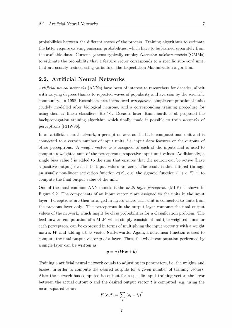
One of the most common ANN models is the multi-layer perceptron (MLP) as shown in

Figure 2.2. The components of an input vector x are assigned to the units in the input

layer. Perceptrons are then arranged in layers where each unit is connected to units from

the previous layer only. The perceptrons in the output layer compute the final output

values of the network, which might be class probabilities for a classification problem. The

feed-forward computation of a MLP, which simply consists of multiple weighted sums for

each perceptron, can be expressed in terms of multiplying the input vector x with a weight

matrix W and adding a bias vector b afterwards. Again, a non-linear function is used to

compute the final output vector y of a layer. Thus, the whole computation performed by

a single layer can be written as

y = � (Wx+ b)

Training a artificial neural network equals to adjusting its parameters, i.e. the weights and

biases, in order to compute the desired outputs for a given number of training vectors.

After the network has computed its output for a specific input training vector, the error

between the actual output o and the desired output vector t is computed, e.g. using the

mean squared error:

E (o, t) =X

i

(oi � ti)2

7

8 2. Background

x1

x2

x3

o1

o2

Hiddenlayer

Inputlayer

Outputlayer

Figure 2.2.: Architecture of a multi-layer perceptron with a single hidden layer.

The backpropagation algorithm is then used to compute first-order gradients for each

weight and bias of the network according to the current error. Gradient descent is com-

monly used to update the parameters by a fraction of their respective gradients. These

steps are usually repeated until convergence on a separate dataset is reached, which means

that the network does not improve its accuracy any more. The MLP training algorithm

used in this work is described in more detail in section 3.2.3.

2.2.1. Tandem Systems for ASR

Throughout the 1980s, a large number of ANN-based speech recognition systems have been

proposed [Lip89]. In particular, work has been done to tackle the problem of recognizing

sequences, for example with Time-Delay Neural Networks [WHH+89] that increase their

temporal context in higher layers by applying low-level hidden units at multiple time steps

to the input, and recurrent neural networks [WS87], in which an internal state is created

by using the output of units as their input again. Although highly successful on limited

tasks, those approaches were eventually abandoned in favor of hidden Markov models

in combination with Gaussian mixtures. In part, this happened because they provided

similar performance to small neural networks and algorithms as well as suitable hardware

for training large networks was lacking.

Afterwards, multiple ways of combining the strengths of both HMMs and ANNs have

been proposed. Bourland & Morgan described a hybrid system that employs neural net-

works for estimating the emission probabilities of sub-word units [BM94]. However, since

modeling emission probabilities with Gaussian mixtures was already established and well-

understood, and the benefits achieved by using neural networks seemed to be rather small,

most researches continued using the GMM/HMM approach. An alternative approach was

proposed in the form of tandem systems, where neural networks are used to generate dis-

criminative input features at the preprocessing stage of an ASR system [FRB97], [HES00].

These features could be integrated into existing systems, which enabled meaningful com-

parisons against setups using standard input features.

In [HES00], Hermansky et al. proposed training a neural network to classify an input vector

8

2.2. Artificial Neural Networks 9

.

.

.

Feature

vector .

.

.

.

.

.

.

.

.

.

.

.

Phoneme

proba-

bilities

Hiddenlayer

Inputlayer

Bottle-neck

Hiddenlayer

Outputlayer

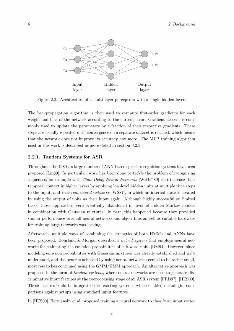
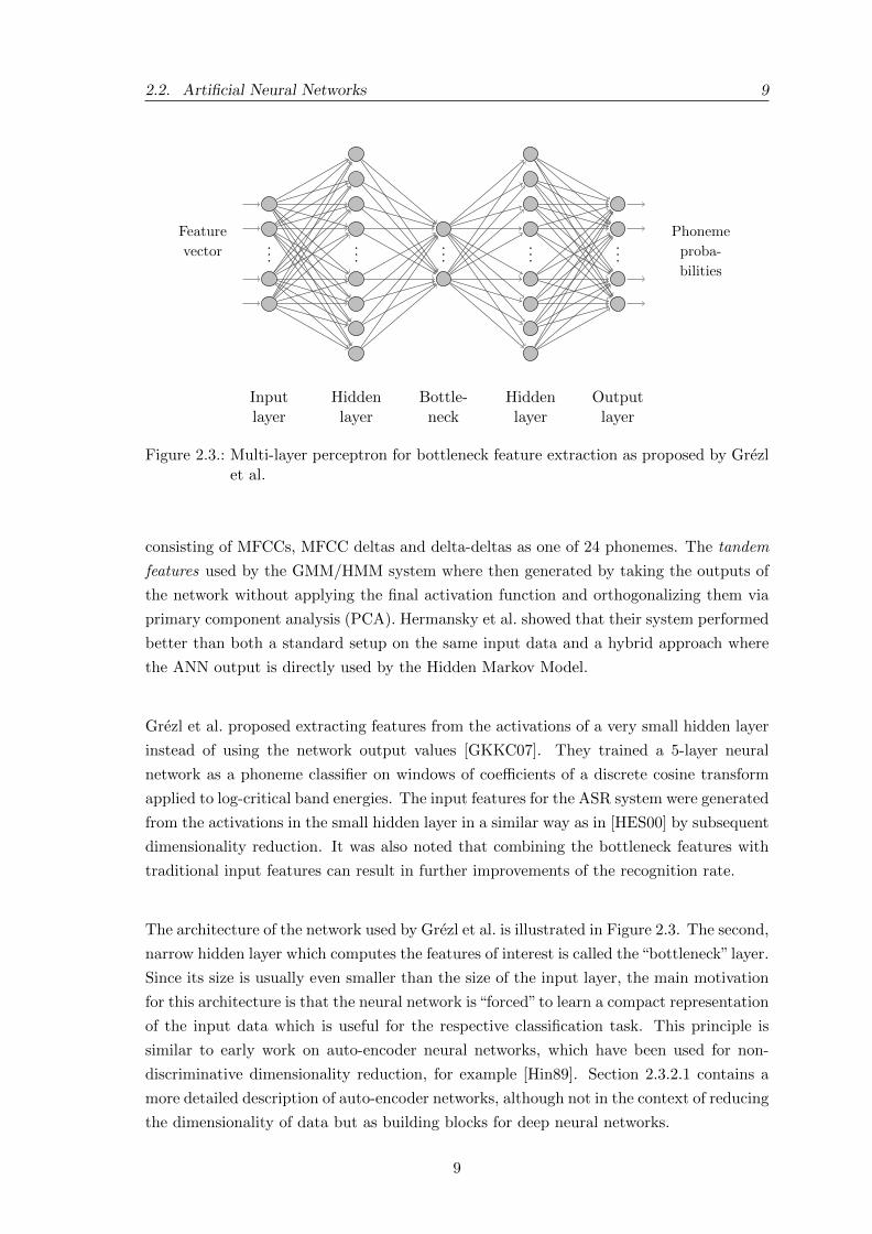
Figure 2.3.: Multi-layer perceptron for bottleneck feature extraction as proposed by Grezlet al.

consisting of MFCCs, MFCC deltas and delta-deltas as one of 24 phonemes. The tandem

features used by the GMM/HMM system where then generated by taking the outputs of

the network without applying the final activation function and orthogonalizing them via

primary component analysis (PCA). Hermansky et al. showed that their system performed

better than both a standard setup on the same input data and a hybrid approach where

the ANN output is directly used by the Hidden Markov Model.

Grezl et al. proposed extracting features from the activations of a very small hidden layer

instead of using the network output values [GKKC07]. They trained a 5-layer neural

network as a phoneme classifier on windows of coe�cients of a discrete cosine transform

applied to log-critical band energies. The input features for the ASR system were generated

from the activations in the small hidden layer in a similar way as in [HES00] by subsequent

dimensionality reduction. It was also noted that combining the bottleneck features with

traditional input features can result in further improvements of the recognition rate.

The architecture of the network used by Grezl et al. is illustrated in Figure 2.3. The second,

narrow hidden layer which computes the features of interest is called the“bottleneck” layer.

Since its size is usually even smaller than the size of the input layer, the main motivation

for this architecture is that the neural network is“forced”to learn a compact representation

of the input data which is useful for the respective classification task. This principle is

similar to early work on auto-encoder neural networks, which have been used for non-

discriminative dimensionality reduction, for example [Hin89]. Section 2.3.2.1 contains a

more detailed description of auto-encoder networks, although not in the context of reducing

the dimensionality of data but as building blocks for deep neural networks.

9

10 2. Background

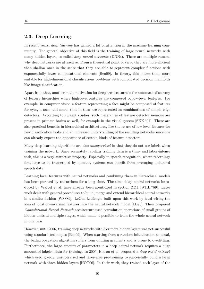
2.3. Deep Learning

In recent years, deep learning has gained a lot of attention in the machine learning com-

munity. The general objective of this field is the training of large neural networks with

many hidden layers, so-called deep neural networks (DNNs). There are multiple reasons

why deep networks are attractive. From a theoretical point of view, they are more e�cient

than shallow ones in the sense that they are able to represent complex functions with

exponentially fewer computational elements [Ben09]. In theory, this makes them more

suitable for high-dimensional classifications problems with complicated decision manifolds

like image classification.

Apart from that, another main motivation for deep architectures is the automatic discovery

of feature hierarchies where high-level features are composed of low-level features. For

example, in computer vision a feature representing a face might be composed of features

for eyes, a nose and more, that in turn are represented as combinations of simple edge

detectors. According to current studies, such hierarchies of feature detector neurons are

present in primate brains as well, for example in the visual system [SKK+07]. There are

also practical benefits in hierarchical architectures, like the re-use of low-level features for

new classification tasks and an increased understanding of the resulting networks since one

can already expect the appearance of certain kinds of feature detectors.

Many deep learning algorithms are also unsupervised in that they do not use labels when

training the network. Since accurately labeling training data is a time- and labor-intense

task, this is a very attractive property. Especially in speech recognition, where recordings

first have to be transcribed by humans, systems can benefit from leveraging unlabeled

speech data.

Learning local features with neural networks and combining them in hierarchical models

has been pursued by researchers for a long time. The time-delay neural networks intro-

duced by Waibel et al. have already been mentioned in section 2.2.1 [WHH+89]. Later

work dealt with general procedures to build, merge and extend hierarchical neural networks

in a similar fashion [WSS89]. LeCun & Bengio built upon this work by hard-wiring the

idea of location-invariant features into the neural network model [LB95]. Their proposed

Convolutional Neural Network architecture used convolution operations of small groups of

hidden units at multiple stages, which made it possible to train the whole neural network

in one pass.

However, until 2006, training deep networks with 3 or more hidden layers was not successful

using standard techniques [Ben09]. When starting from a random initialization as usual,

the backpropagation algorithm su↵ers from diluting gradients and is prone to overfitting.

Furthermore, the large amount of parameters in a deep neural network requires a huge

amount of labeled data for training. In 2006, Hinton et al. proposed a deep belief network

which used greedy, unsupervised and layer-wise pre-training to successfully build a large

network with three hidden layers [HOT06]. In their work, they trained each layer of the

10

2.3. Deep Learning 11

network as a restricted Boltzmann machine (RBM) [AHS85]. Their key insight was that

unsupervised training can be used to initialize each layer in a local, isolated fashion and

that the resulting network can be trained much easier than starting with random weights.

The major part of the work in deep learning makes use of the layer-wise pre-training

strategy of Hinton et al. as well. Bengio et al. showed that auto-encoder networks can

be used for pre-training instead of restricted Boltzmann machines [BLPL07]. Shortly

afterwards, sparse models have been proposed that increase the invariance of learnt features

[MRBL07]. Building on earlier ideas by LeCun et al., Lee et al. developed location-

and time-invariant convolutional models that can be pre-trained accordingly, focussing

explicitly on the ability of hierarchical feature extraction [LGRN09]. Quite recently, those

ideas ideas have been applied to harder, large-scale problems and led to breakthroughs in

speech recognition [SLY11], [DYDA12], object recognition [LMD+11], [KSH12] and other

areas. The following section provides a more detailed overview of current work on applying

deep learning to acoustic modeling for ASR.

In order to build deep neural networks, the work at hand utilizes an alternative auto-

encoder model proposed by Vincent et al. [VLBM08] which will be introduced section 2.3.2.

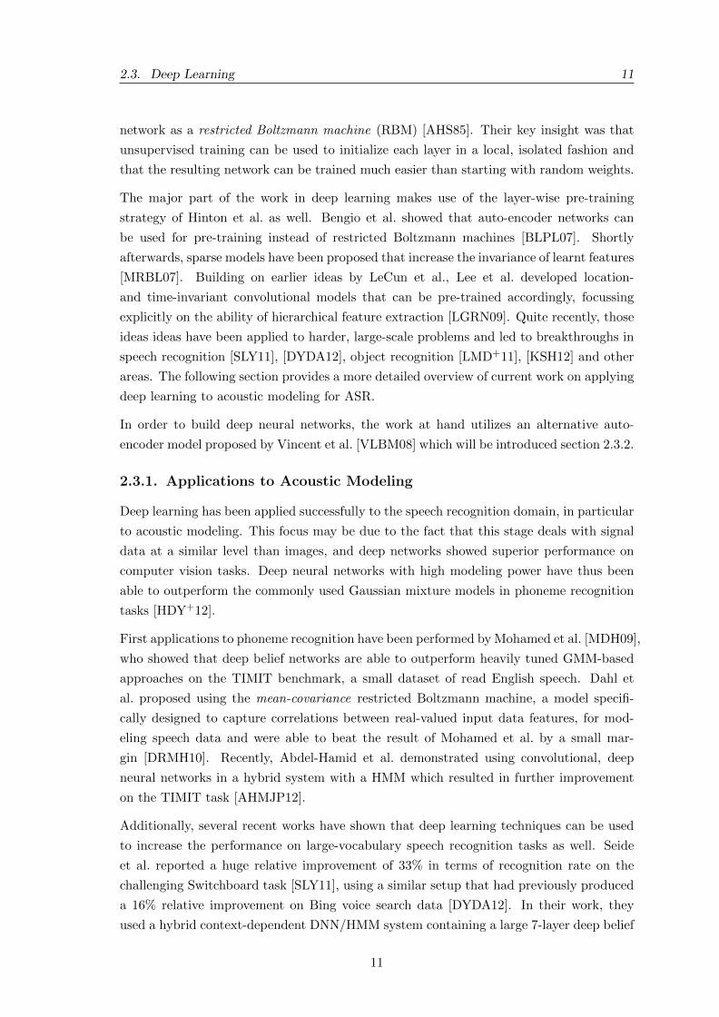
2.3.1. Applications to Acoustic Modeling

Deep learning has been applied successfully to the speech recognition domain, in particular

to acoustic modeling. This focus may be due to the fact that this stage deals with signal

data at a similar level than images, and deep networks showed superior performance on

computer vision tasks. Deep neural networks with high modeling power have thus been

able to outperform the commonly used Gaussian mixture models in phoneme recognition

tasks [HDY+12].

First applications to phoneme recognition have been performed by Mohamed et al. [MDH09],

who showed that deep belief networks are able to outperform heavily tuned GMM-based

approaches on the TIMIT benchmark, a small dataset of read English speech. Dahl et

al. proposed using the mean-covariance restricted Boltzmann machine, a model specifi-

cally designed to capture correlations between real-valued input data features, for mod-

eling speech data and were able to beat the result of Mohamed et al. by a small mar-

gin [DRMH10]. Recently, Abdel-Hamid et al. demonstrated using convolutional, deep

neural networks in a hybrid system with a HMM which resulted in further improvement

on the TIMIT task [AHMJP12].

Additionally, several recent works have shown that deep learning techniques can be used

to increase the performance on large-vocabulary speech recognition tasks as well. Seide

et al. reported a huge relative improvement of 33% in terms of recognition rate on the

challenging Switchboard task [SLY11], using a similar setup that had previously produced

a 16% relative improvement on Bing voice search data [DYDA12]. In their work, they

used a hybrid context-dependent DNN/HMM system containing a large 7-layer deep belief

11

12 2. Background

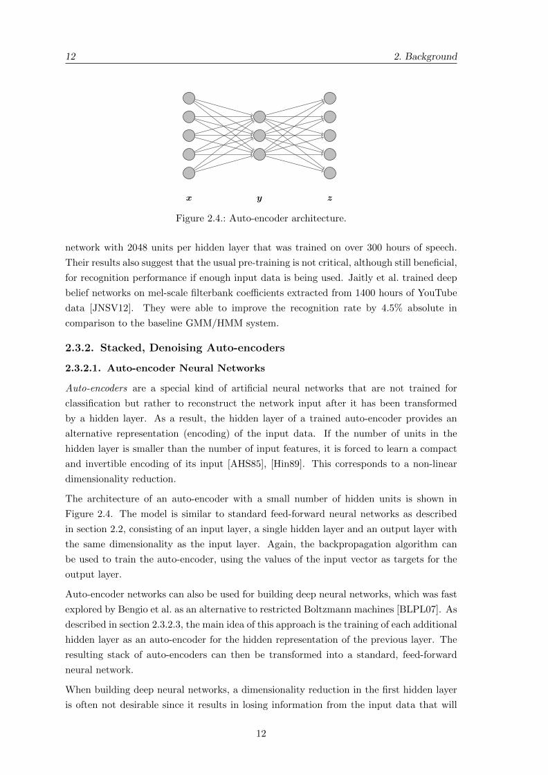
x y z

Figure 2.4.: Auto-encoder architecture.

network with 2048 units per hidden layer that was trained on over 300 hours of speech.

Their results also suggest that the usual pre-training is not critical, although still beneficial,

for recognition performance if enough input data is being used. Jaitly et al. trained deep

belief networks on mel-scale filterbank coe�cients extracted from 1400 hours of YouTube

data [JNSV12]. They were able to improve the recognition rate by 4.5% absolute in

comparison to the baseline GMM/HMM system.

2.3.2. Stacked, Denoising Auto-encoders

2.3.2.1. Auto-encoder Neural Networks

Auto-encoders are a special kind of artificial neural networks that are not trained for

classification but rather to reconstruct the network input after it has been transformed

by a hidden layer. As a result, the hidden layer of a trained auto-encoder provides an

alternative representation (encoding) of the input data. If the number of units in the

hidden layer is smaller than the number of input features, it is forced to learn a compact

and invertible encoding of its input [AHS85], [Hin89]. This corresponds to a non-linear

dimensionality reduction.

The architecture of an auto-encoder with a small number of hidden units is shown in

Figure 2.4. The model is similar to standard feed-forward neural networks as described

in section 2.2, consisting of an input layer, a single hidden layer and an output layer with

the same dimensionality as the input layer. Again, the backpropagation algorithm can

be used to train the auto-encoder, using the values of the input vector as targets for the

output layer.

Auto-encoder networks can also be used for building deep neural networks, which was fast

explored by Bengio et al. as an alternative to restricted Boltzmann machines [BLPL07]. As

described in section 2.3.2.3, the main idea of this approach is the training of each additional

hidden layer as an auto-encoder for the hidden representation of the previous layer. The

resulting stack of auto-encoders can then be transformed into a standard, feed-forward

neural network.

When building deep neural networks, a dimensionality reduction in the first hidden layer

is often not desirable since it results in losing information from the input data that will

12


be missing when training consecutive layers. Instead, the auto-encoder used for the first

layer should learn an over-complete representation of its input by having more hidden

units than input features. Another motivation for learning a high-dimensionality is that

this way, models can learn to disentangle the factors of variation present in the original

data [VLL+10]. Subsequent models and classifiers might then benefit from such a dis-

entangled representation, where the individual factors extracted can be combined again.

However, care must be taken to prevent an over-complete model from learning a trivial

identity-like mapping in which every hidden unit is activated by only one input feature. A

common technique for learning useful over-complete representations in the context of deep

learning includes the addition of a sparsity constraint that forces most of the hidden units

to have near-zero activation given a particular training example [MRCL06], [MRBL07].

2.3.2.2. Adding a Denoising Criterion

An alternative approach to extend classic auto-encoders for deep learning purposes has

been proposed by Vincent et al. [VLBM08]. In a so-called denoising auto-encoder (DAE),

the input data is first corrupted by applying random noise to the individual features.

Afterwards, the model is trained to reconstruct the uncorrupted input from the corrupted

input in an auto-encoder-like fashion. In their work, Vincent et al. showed that hidden

representations learned from randomly corrupted input di↵er from the results achieved

with standard sparsity constraints and may provide more useful features when adding

further layers.

The general idea of adding noise to training examples in order to improve the general-

ization ability of a neural network is much older. In 1986, Plaut, Nowlan and Hinton

added Gaussian noise to artificial data resembling speech signals and reported excellent

results [PNH86], but did not perform a direct omparison to training without noise. This

was done in numerous further experiments, for example by Elmand and Zipser [EZ88] or

Sietsma and Dow [SD91] who could confirm an increased generalization when adding noise

to the input data of a network.

Deep neural networks constructed from denoising auto-encoders have been used for image

recognition [VLL+10], natural language processing [DGB11] and text sentiment classifi-

cation [GBB11], for example, with results that demonstrated the competitiveness of the

approach compared to other deep learning concepts like deep belief networks. Denoising

auto-encoders are also used as the main building blocks in this work, and will be described

in more detail in the following.

The individual steps of the computation performed by a denoising auto-encoder are illus-

trated in Figure 2.5. As noted above, the main di↵erence to normal auto-encoders is the

corruption of an input vector x. This can be formalized as the application of a stochastic

process qD

x ⇠ qD(x|x)

13

14 2. Background

Corruption Auto-encoder

x x y z

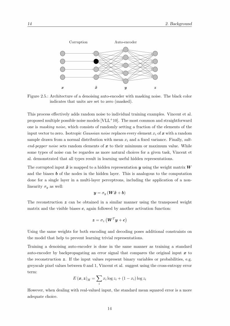
Figure 2.5.: Architecture of a denoising auto-encoder with masking noise. The black colorindicates that units are set to zero (masked).

This process e↵ectively adds random noise to individual training examples. Vincent et al.

proposed multiple possible noise models [VLL+10]. The most common and straightforward

one is masking noise, which consists of randomly setting a fraction of the elements of the

input vector to zero. Isotropic Gaussian noise replaces every element xi of x with a random

sample drawn from a normal distribution with mean xi and a fixed variance. Finally, salt-

end-pepper noise sets random elements of x to their minimum or maximum value. While

some types of noise can be regardes as more natural choices for a given task, Vincent et

al. demonstrated that all types result in learning useful hidden representations.

The corrupted input x is mapped to a hidden representation y using the weight matrix W

and the biases b of the nodes in the hidden layer. This is analogous to the computation

done for a single layer in a multi-layer perceptrons, including the application of a non-

linearity �y as well:

y = �y (Wx+ b)

The reconstruction z can be obtained in a similar manner using the transposed weight

matrix and the visible biases c, again followed by another activation function:

z = �z

�W

Ty + c

�

Using the same weights for both encoding and decoding poses additional constraints on

the model that help to prevent learning trivial representations.

Training a denoising auto-encoder is done in the same manner as training a standard

auto-encoder by backpropagating an error signal that compares the original input x to

the reconstruction z. If the input values represent binary variables or probabilities, e.g.

greyscale pixel values between 0 and 1, Vincent et al. suggest using the cross-entropy error

term:

E (x, z)H =X

i

xi log zi + (1� xi) log zi

However, when dealing with real-valued input, the standard mean squared error is a more

adequate choice.

14


yx

x

0x

0y

0z

0

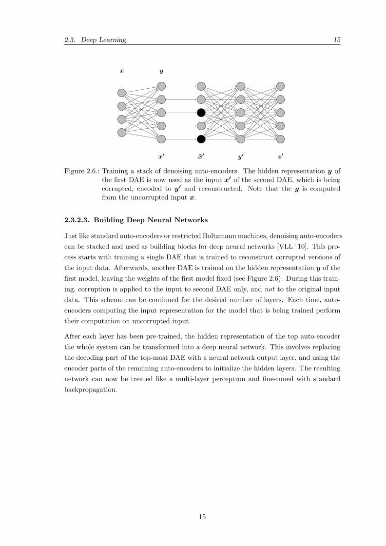
Figure 2.6.: Training a stack of denoising auto-encoders. The hidden representation y ofthe first DAE is now used as the input x0 of the second DAE, which is beingcorrupted, encoded to y

0 and reconstructed. Note that the y is computedfrom the uncorrupted input x.

2.3.2.3. Building Deep Neural Networks

Just like standard auto-encoders or restricted Boltzmann machines, denoising auto-encoders

can be stacked and used as building blocks for deep neural networks [VLL+10]. This pro-

cess starts with training a single DAE that is trained to reconstruct corrupted versions of

the input data. Afterwards, another DAE is trained on the hidden representation y of the

first model, leaving the weights of the first model fixed (see Figure 2.6). During this train-

ing, corruption is applied to the input to second DAE only, and not to the original input

data. This scheme can be continued for the desired number of layers. Each time, auto-

encoders computing the input representation for the model that is being trained perform

their computation on uncorrupted input.

After each layer has been pre-trained, the hidden representation of the top auto-encoder

the whole system can be transformed into a deep neural network. This involves replacing

the decoding part of the top-most DAE with a neural network output layer, and using the

encoder parts of the remaining auto-encoders to initialize the hidden layers. The resulting

network can now be treated like a multi-layer perceptron and fine-tuned with standard

backpropagation.

15

Bottleneck Features from Deep Neural

Networks

3.1. Previous Work

For the most part, work on applying deep neural networks to automatic speech recognition

dealt with refining acoustic models and language models, and significant improvements

could be achieved in those areas. As of now, only few publications examined how tandem

systems using probabilistic or bottleneck features could be improved with deep learning

techniques.

In 2011, Yu & Seltzer pre-trained restricted Boltzmann machines (RBMs) in the usual

fashion to form deep belief network for supervised phoneme classification from MFCC

input including deltas and delta-deltas [YS11]. They proposed a symmetric architecture

where the bottleneck layer is surrounded by an equal number of large, hidden layers on both

sides. In their work, they evaluated the e↵ects of pre-training and of using di↵erent kinds of

labels for supervised training on a business voice search task containing 24 hours of speech.

It was shown that unsupervised pre-training resulted in higher recognition accuracy of the

whole system, and that using context-dependent senones instead of monophone targets for

supervised fine-tuning improved the recognition rate significantly. However, their model

failed to profit as expected from increasing the number of hidden layers. They noted

that this may be due to their symmetric architecture in which the bottleneck is separated

by possibly numerous hidden layers from the classification layer, and therefore receives

only weak gradients from the current error. In a more recent work, Mohamed et al. also

argued that RBMs are unsuited for modeling highly decorrelated data such as MFCCs and

suggested training on log mel scale filterbank coe�cients instead [MHP12].

Sainath et al. applied deep belief networks to an auto-encoder bottleneck architecture

proposed by Mangu et al. [MKC+11], [SKR12]. First, they trained a DBN to predict

16

3.2. Model Description and Training Procedure 17

clustered, context-dependent targets given a frame of speaker-adapted PLP features. Af-

terwards, they trained an auto-encoder network on the DBN outputs that reduced its input

data in two steps to 40 features, which were then used as input for the speech recognition

system. Their evaluation on two English broadcast news tasks containing 50 and 430 hours

of speech resulted in absolute improvements of 1.0% and 0.5% in terms of word error rate

over strong baseline systems using the same input features.

In both works, deep learning techniques known to work well on speech data have been

directly transfered to tasks previously done by shallow networks obtained by supervised

training. This showed the general applicability of these methods and produced valuable

insights, e.g. for selecting the targets used for fine-tuning. However, this thesis proposes a

di↵erent training procedure that combines the advantages of deep neural networks and di-

mensionality reduction by supervised training. This is done by training a network contain-

ing a bottleneck layer in a supervised manner once a deep, high-dimensional representation

of the data has been obtained via unsupervised, layer-wise pre-training.

The model for pre-training layers that was selected for this thesis are denoising auto-

encoders as described in section 2.3.2. Previous work by Vincent et al. demonstrated their

ability to model sound in the context of music genre classification [VLL+10]. Apart from

that, I am not aware of any previous work on applying the DAE concept to audio data,

in particular to speech recognition.

Most of the work on deep learning for speech recognition was done using deep belief

networks built from restricted Boltzmann machines, e.g. acoustic modeling in hybrid

DBN/HMM setups (see section 2.3.1). The reasons for choosing denoising auto-encoders

instead of an already tested approach for this work are the following: first, training re-

stricted Boltzmann machines on real-valued input like speech is more di�cult than on

binary data for which they were originally proposed, in the sense that the training algo-

rithm is not very robust and care must be taken to sensibly select correct hyper-parameters

like the learning rate and to normalize the input data [Hin10]. Second, this work initially

focussed on extracting bottleneck features from MFCC data, which was argued to be un-

suitable for training RBMs with [MHP12]. Last, the theoretical and practical simplicity

of the auto-encoder setup is appealing, and it was interesting to prove their applicability

to model speech data.

3.2. Model Description and Training Procedure

The proposed architecture for bottleneck feature extraction is illustrated in Figure 3.1.

First, a number of equally-sized layer is pre-trained as denoising auto-encoders in a greedy,

unsupervised fashion in order to generate a useful deep representation of the input data.

This is the usual procedure when pre-training a deep neural network that might be used

for classification later. Afterwards, a small bottleneck layer, an additional hidden layer and

a classification layer are added. The whole model is then fine-tuned to predict phonetic

17

18 3. Bottleneck Features from Deep Neural Networks

Bottleneck

Auto-encoders

Hidden Classification

layer layer

Speech

input

Stacked

1000

1000

1000

1000

42

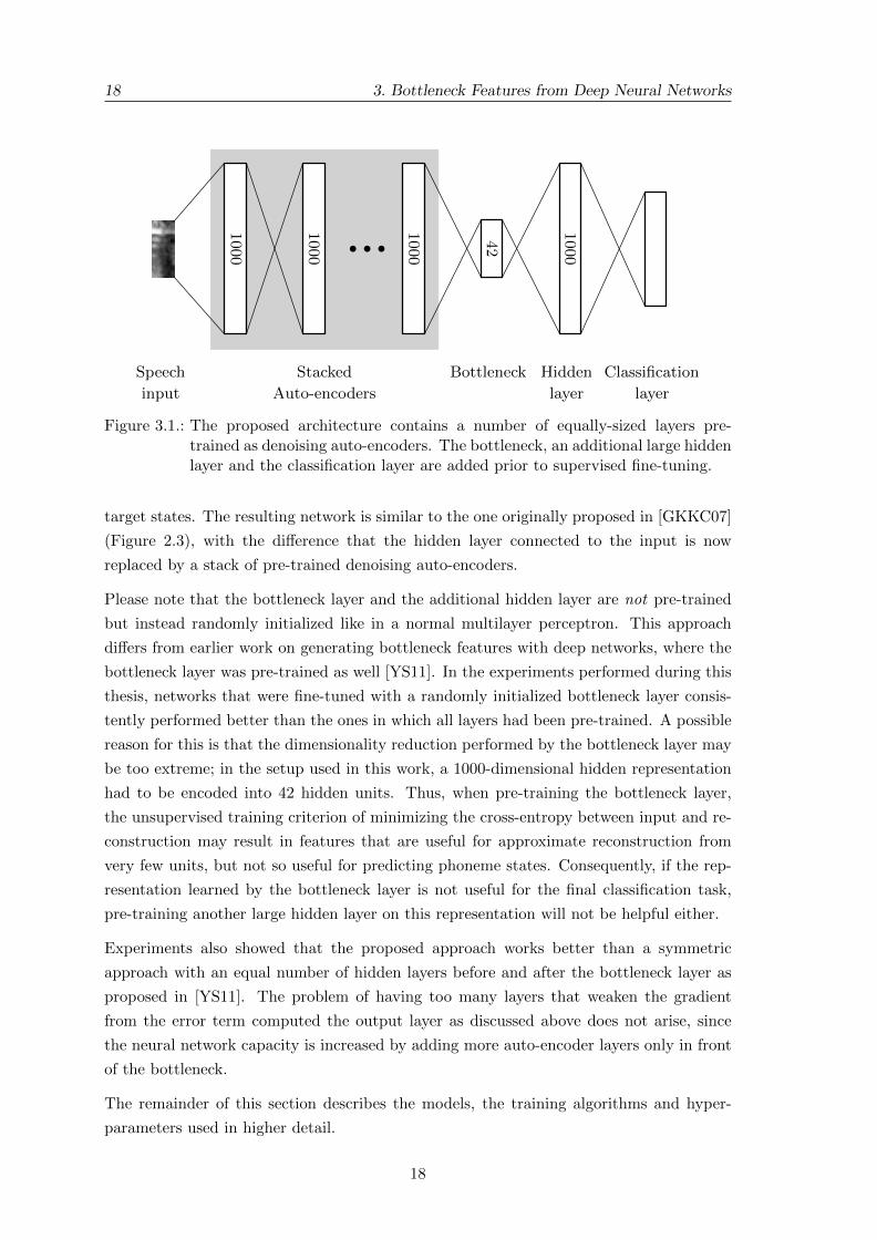
Figure 3.1.: The proposed architecture contains a number of equally-sized layers pre-trained as denoising auto-encoders. The bottleneck, an additional large hiddenlayer and the classification layer are added prior to supervised fine-tuning.

target states. The resulting network is similar to the one originally proposed in [GKKC07]

(Figure 2.3), with the di↵erence that the hidden layer connected to the input is now

replaced by a stack of pre-trained denoising auto-encoders.

Please note that the bottleneck layer and the additional hidden layer are not pre-trained

but instead randomly initialized like in a normal multilayer perceptron. This approach

di↵ers from earlier work on generating bottleneck features with deep networks, where the

bottleneck layer was pre-trained as well [YS11]. In the experiments performed during this

thesis, networks that were fine-tuned with a randomly initialized bottleneck layer consis-

tently performed better than the ones in which all layers had been pre-trained. A possible

reason for this is that the dimensionality reduction performed by the bottleneck layer may

be too extreme; in the setup used in this work, a 1000-dimensional hidden representation

had to be encoded into 42 hidden units. Thus, when pre-training the bottleneck layer,

the unsupervised training criterion of minimizing the cross-entropy between input and re-

construction may result in features that are useful for approximate reconstruction from

very few units, but not so useful for predicting phoneme states. Consequently, if the rep-

resentation learned by the bottleneck layer is not useful for the final classification task,

pre-training another large hidden layer on this representation will not be helpful either.

Experiments also showed that the proposed approach works better than a symmetric

approach with an equal number of hidden layers before and after the bottleneck layer as

proposed in [YS11]. The problem of having too many layers that weaken the gradient

from the error term computed the output layer as discussed above does not arise, since

the neural network capacity is increased by adding more auto-encoder layers only in front

of the bottleneck.

The remainder of this section describes the models, the training algorithms and hyper-

parameters used in higher detail.

18


3.2.1. Denoising Auto-Encoders for Speech

In their application of denoising auto-encoders to classification of music genres, Vincent

et al. proposed modifying the decoding part of the model accordingly [VLL+10]. They

did not apply the usual sigmoid activation function to the output units that make up the

reconstruction, which resulted in a linear decoder. Furthermore, since audio data is usu-

ally real-valued, they computed the minimum squared error (MSE) between uncorrupted

input and linear decoded output in order to generate an error signal for training. These

adaptations were applied to the first auto-encoder only, though. Since the sigmoid activa-

tion function was still used to compute the values of the hidden units, the input data for

the second and subsequent auto-encoders could be considered as representing probabili-

ties, which made it possible to employ the usual combination of sigmoid output units and

cross-entropy error training.

In this work, denoising auto-encoders were used to model both MFCC and log mel scale

(lMEL) filterbank data, which was extracted from audio data as described in section 3.3.1.

After a set of initial experiments on MFCC data were performed, the linear activation of

the output units was abandoned in favor of a hyperbolic tangent activation. This seemed

suitable, since MFCCs are commonly distributed in a Gaussian-like fashion around 0, and

the data at hand had only few outliers with values outside of the [�1, 1] interval. Training

with a non-linearity in the decoder also resulted in more stable results regarding the setting

of di↵erent hyper-parameters. For the lMEL data, which was introduced later in the thesis

work, the same model properties were selected and worked well regardless of the slightly

di↵erent input distribution.

The first DAE employing the tanh activation function for its output units was trained

to minimize the mean squared error of its reconstruction, while subsequent auto-encoders

were trained using the cross-entropy error term. Following the standard approach, those

models used the sigmoid activation function for their output units.

As mentioned in section 2.3.2, it is desirable to learn an over-complete representation from

the input when pre-training layers to be used in a deep neural network. At the start of

this thesis, several values for the number of hidden units in the first auto-encoder were

tested. Using 1000 hidden units turned out to be a good compromise, since smaller layers

performed worse and adding more hidden units did not result in significant improvements

on the development system but in much longer training time, especially for networks with

many hidden layers.

3.2.2. Layer-wise Pre-training

The auto-encoder layers were pre-trained as denoising auto-encoders, each one trained to

encode the hidden representation of the previous one (or the input data, in case of the

first DAE). All training steps used the same hyper-parameters, except for the error term

used to compute gradient updates as discussed above. Prior to training, the weights of an

19


auto-encoder where initialized randomly depending on the size of the model. As suggested

by Glorot & Bengio, weights were sampled from a uniform distribution within the intervalh� 1p

n,

1pn

i, where n equals to the number of visible and hidden units of the model [GB10].

The bias values of the visible and hidden units were all set to zero.

For corrupting the input of the denoising auto-encoder, 20% masking noise was applied

to the data, resulting in a random fraction of 20% of input elements being set to zero.

As already noted in [VLL+10], changing the number of corrupted elements changes the

resulting filters (the weight values can be interpreted as detectors for certain input pat-

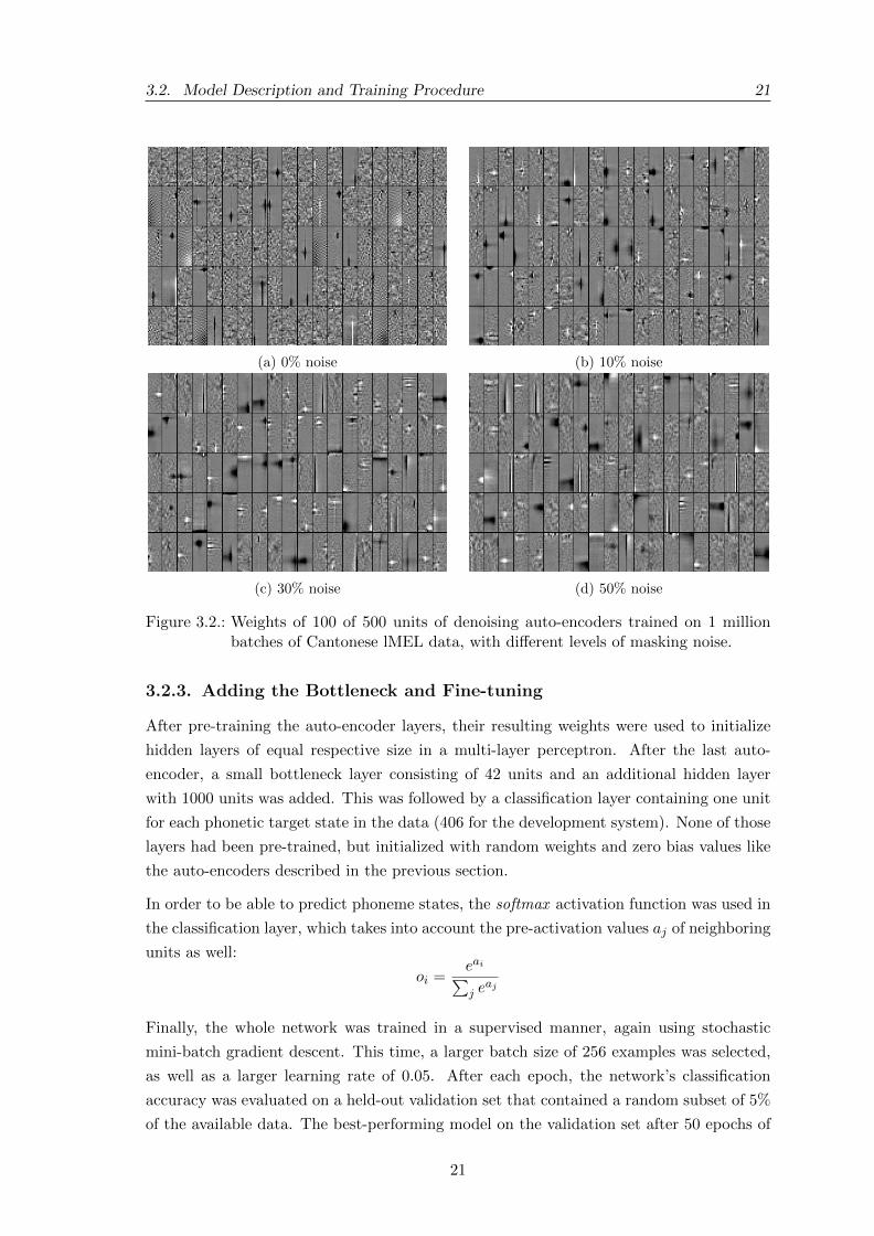
terns). Figure 3.2 shows a comparison of learned filters when using di↵erent noise levels

on lMEL data. The images were generated by plotting the weights of selected hidden units

in input space, where a dark pixel indicates a negative weight for the connection of a unit

to the respective input element, and a light pixel indicates a positive weight. The weight

values were clipped so that white corresponds to a value of 0.5 or higher, black to -0.5 or

lower and grey to 0. For the purpose of visualization, the input space is assumed to be

two-dimensional: each row inside a rectangle corresponds to a specific frequency on the

mel scale. Samples are arranged in columns to form the frames used for network training.

It can be seen that less noise results in more local and more noise in more global filters,

which is consistent with the results reported in [VLL+10]. The figure also shows that

without applying any noise during training, the model has a hard time learning plausible

filters.

Auto-encoder training was done using stochastic mini-batch gradient descent as described

in appendix A.3, with a batch size of 64 and a learning rate of 0.01. Each layer was pre-

trained on 4 million mini-batches, which resulted in 4 million updates on each parameter

and a total of 256 million training examples used (including duplicates caused by iterating

multiple times over the dataset). The 44 hours of training data for the development system

described in section 4.1.2.1 resulted in a dataset containing about 17 million frames, so

slightly more than 15 epochs were needed for pre-training in this case.

The relatively short duration of pre-training with a small learning rate was selected in

order to prevent overfitting of the models, which was observed in the form of hidden units

that react to only one input feature (Figure 3.3). This tendency emerged in units that

did not manage to capture a plausible filter in the beginning. While these detectors might

lower the reconstruction error by a tiny margin, they usually indicate a degraded unit

not suitable for classification. Additionally, since the data contained outliers not in the

image of the tanh activation function used for the visible units of the first auto-encoder,

it was desirable to limit the impact of the error signal from those points. This would

especially occur later during training, when most of the weights had settled and failure in

reconstructing single points would become more apparent.

20


(a) 0% noise (b) 10% noise

(c) 30% noise (d) 50% noise

Figure 3.2.: Weights of 100 of 500 units of denoising auto-encoders trained on 1 millionbatches of Cantonese lMEL data, with di↵erent levels of masking noise.

3.2.3. Adding the Bottleneck and Fine-tuning

After pre-training the auto-encoder layers, their resulting weights were used to initialize

hidden layers of equal respective size in a multi-layer perceptron. After the last auto-

encoder, a small bottleneck layer consisting of 42 units and an additional hidden layer

with 1000 units was added. This was followed by a classification layer containing one unit

for each phonetic target state in the data (406 for the development system). None of those

layers had been pre-trained, but initialized with random weights and zero bias values like

the auto-encoders described in the previous section.

In order to be able to predict phoneme states, the softmax activation function was used in

the classification layer, which takes into account the pre-activation values aj of neighboring

units as well:

oi =e

ai

Pj e

aj

Finally, the whole network was trained in a supervised manner, again using stochastic

mini-batch gradient descent. This time, a larger batch size of 256 examples was selected,

as well as a larger learning rate of 0.05. After each epoch, the network’s classification

accuracy was evaluated on a held-out validation set that contained a random subset of 5%

of the available data. The best-performing model on the validation set after 50 epochs of

21


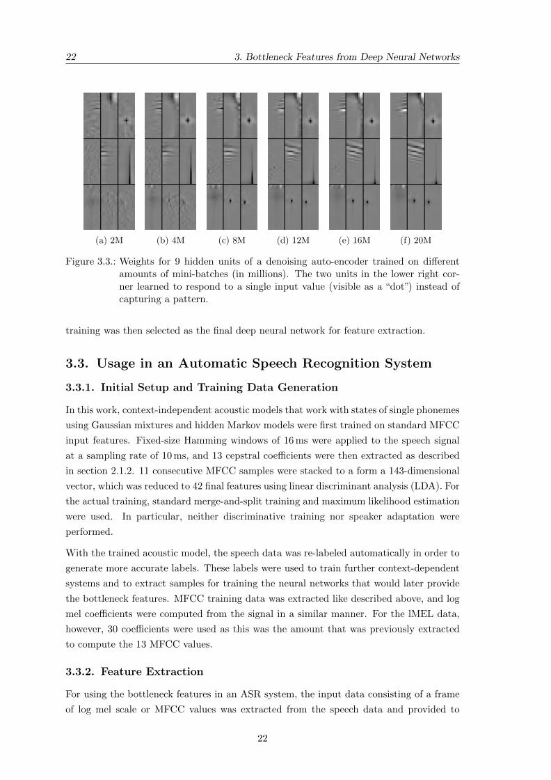
(a) 2M (b) 4M (c) 8M (d) 12M (e) 16M (f) 20M

Figure 3.3.: Weights for 9 hidden units of a denoising auto-encoder trained on di↵erentamounts of mini-batches (in millions). The two units in the lower right cor-ner learned to respond to a single input value (visible as a “dot”) instead ofcapturing a pattern.

training was then selected as the final deep neural network for feature extraction.

3.3. Usage in an Automatic Speech Recognition System

3.3.1. Initial Setup and Training Data Generation

In this work, context-independent acoustic models that work with states of single phonemes

using Gaussian mixtures and hidden Markov models were first trained on standard MFCC

input features. Fixed-size Hamming windows of 16ms were applied to the speech signal

at a sampling rate of 10ms, and 13 cepstral coe�cients were then extracted as described

in section 2.1.2. 11 consecutive MFCC samples were stacked to a form a 143-dimensional

vector, which was reduced to 42 final features using linear discriminant analysis (LDA). For

the actual training, standard merge-and-split training and maximum likelihood estimation

were used. In particular, neither discriminative training nor speaker adaptation were

performed.

With the trained acoustic model, the speech data was re-labeled automatically in order to

generate more accurate labels. These labels were used to train further context-dependent

systems and to extract samples for training the neural networks that would later provide

the bottleneck features. MFCC training data was extracted like described above, and log

mel coe�cients were computed from the signal in a similar manner. For the lMEL data,

however, 30 coe�cients were used as this was the amount that was previously extracted

to compute the 13 MFCC values.

3.3.2. Feature Extraction

For using the bottleneck features in an ASR system, the input data consisting of a frame

of log mel scale or MFCC values was extracted from the speech data and provided to

22

3.3. Usage in an Automatic Speech Recognition System 23

the network. The values of the hidden units in the bottleneck layer are computed and

then used as a feature vector for the GMM/HMM acoustic model. In order to get good,

decorrelated features, a whole frame of consecutive bottleneck features is extracted and

reduced via LDA.

In the setups used in this thesis, the network was trained to extract 42 bottleneck features.

The feature vector was formed using a context of 5 past and 5 future samples, resulting in

a total of 11 · 42 = 462 bottleneck features that were then reduced to 42 features as with

the standard MFCC data.

The bottleneck features were used to train context-dependent acoustic models only. Initial

attempts to use BNFs for context-independent training had failed, presumably because of

the di↵erent feature space compared to MFCCs. This would have required adjusting

the parameters used for generating the polyphone decision tree determining the tying

of context-dependent phone states. However, since negligible e↵ects were anticipated by

training a context-independent system on bottleneck features, no further work was done

to adopt the context clustering stage accordingly.

23

Experiments

4.1. Baseline Systems

4.1.1. The Janus Recognition Toolkit

For all the experiments performed in this thesis, the Janus recognition toolkit (JRTk,

[FGH+97]) was used to extract speech data and to train and evaluate the speech recognition

systems. The JRTk provides a flexible architecture for building state-of-the-art recognition

systems, with the actual computational flow being determined by Tcl scripts. The actual

decoding to determine the performance of the systems trained was done using the IBIS

decoder, which is included in the recognition toolkit [SMFW01].

4.1.2. System Configurations

In the following, the individual datasets, acoustic model setups and language models will

be described that were used for developing, optimizing and evaluating the proposed archi-

tecture. Recognition performance of the respective baseline systems using MFCC features

is stated as well; please refer to section 4.2 for an explanation of the performance measures

used.

4.1.2.1. Development System

The initial experiments regarding network architectures and the optimization of hyper-

parameters for neural network training were performed on a comparably small development

system. The corresponding dataset consisted of 44 hours of conversational telephone speech

from 400 speakers in Cantonese, a language natively spoken in southern pars of China as

well as Hong Kong and Macao. This corpus was recently released with identifier “101A”

during the IARPA BABEL program [IAR], and is a subset of the full Cantonese dataset

“101B” containing 80 hours of speech from 966 speakers.

24

4.1. Baseline Systems 25

Acoustic model training for the context-independent system was done as described in

section 3.3.1, using MFCC input data and maximum likelihood training. The data used

for neural network training was labeled with three states for each phoneme (begin, middle

and end), resulting in a total of 406 phonetic targets for this setup.

For the development system, a simple 3-gram language model was used, in which the

probability of a single word occurring in a sequence is determined by the two words that

appear in front of it. The model was extracted from the transcriptions that had been

provided with the data.

The baseline system used as a reference in recognition performance was among the initial

system builds on this new and relatively small corpus. With the simple language model

described above and using only basic acoustic model training, it achieved a character error

rate (CER) of 71.5%. This number was determined by transcribing data from a testing

set containing 3.3 hours of speech.

4.1.2.2. Cantonese

Further experiments for optimizing the network architecture were performed on the full

“101B” dataset of Cantonese with 80 hours of speech. This system employed a more

sophisticated language model, again using 3-grams but interpolating between the corpus

data and text extracted from Cantonese Wikipedia articles. The recognition performance

of the baseline on MFCC features was 66.4% CER, using a much larger testing set with

20 hours of speech.

4.1.2.3. Tagalog

The Tagalog corpus is another new dataset released by IARPA for the BABEL program,

identified as “106B” and containing conversational telephone speech, too. Tagalog is the

native language spoken in large parts of the Philippines. In total, the dataset consisted of

69 hours of speech. The system setup was similar to the one used for the full Cantonese

dataset and also used a language model interpolating between transcriptions contained in

the corpus and text from Wikipedia articles. The baseline system achieved a word error

rate (WER) of 72.5% on a test set of 24 hours.

4.1.2.4. Switchboard

In order to evaluate the bottleneck feature setup on a more standard benchmark, an

additional system was trained on the Switchboard task [GHM92]. This corpus contains

300 hours of English conversational telephone speech, and is widely used as a benchmark

for speech-to-text transcription in the ASR community. As for the development system,

acoustic models were trained using maximum likelihood estimation and Viterbi training

only. Similarly, the language model used 3-grams extracted from the corpus transcriptions.

The MFCC-based baseline system resulted in 39.0% WER.

25

26 4. Experiments

4.2. Evaluation Criteria

Even though the neural networks used for bottleneck feature extraction were trained to

minimize a classification error, their actual classification performance was not of much

interest. Instead, networks were compared on the basis of the recognition accuracy that

can be achieved by using the generated features. While the classification accuracy of a

network in comparison to another one on the same dataset might give hints about the

quality of its bottleneck features, training acoustic models and performing decoding on

the test set is needed to produce a final result.

The ASR systems used in this work generally measured the recognition performance in

word error rate (WER). The goal is to measure the di↵erence between the text sequence

generated by the system and a reference transcription, which may di↵er in contents as well

as in length. Thus, the word error rate is computed by summing up the word substitutions,

insertions and deletions that need to be performed to transform the system output into

the reference transcription, normalized by the number of words in the reference:

WER =#Substitutions + #Insertions + #Deletions

#Words in reference

There is no clear concept of a single word in Cantonese, so the word error rate which relies

on word boundary detection is not a very useful performance metric there. Instead, the

character error rate (CER), which is computed in an analogous manner, was used for the

respective systems.

4.3. Experiments on the Development System

The first experiments that have been performed mostly dealt with exploring di↵erent types

of architectures for bottleneck feature extraction as well as di↵erent pre-training schemes.

A high-level summary of the relevant outcomes that led to the design decisions made in

this thesis is included in the model description in section 3.2. This section describes the

systematic comparisons performed after basic model properties and hyper-parameters had

already been selected.

4.3.1. Input Data

As noted previously, the proposed architecture was trained to extract bottleneck features

from both MFCCs and log mel scale filterbank coe�cients (lMEL). In the case of restricted

Boltzmann machines, Mohamed et al. argued that MFCCs are unsuited because of their

decorrelated nature [MHP12]. Although this limitation was not specifically stated for

denoising auto-encoders as used in this work, the idea of applying random corruption

to the input values is in part aiming at the discovery of relations between the di↵erent

elements of an input vector as well.

26

4.3. Experiments on the Development System 27

65

66

67

68

69

70

71

72

1 2 3 4 5

CE

R (

%)

Number of auto-encoder layers

MFCC baseline

lMEL MFCC

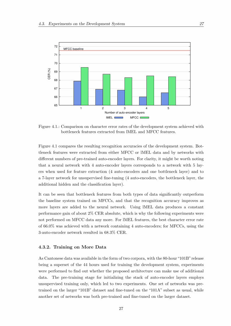
Figure 4.1.: Comparison on character error rates of the development system achieved withbottleneck features extracted from lMEL and MFCC features.

Figure 4.1 compares the resulting recognition accuracies of the development system. Bot-

tleneck features were extracted from either MFCC or lMEL data and by networks with

di↵erent numbers of pre-trained auto-encoder layers. For clarity, it might be worth noting

that a neural network with 4 auto-encoder layers corresponds to a network with 5 lay-

ers when used for feature extraction (4 auto-encoders and one bottleneck layer) and to

a 7-layer network for unsupervised fine-tuning (4 auto-encoders, the bottleneck layer, the

additional hidden and the classification layer).

It can be seen that bottleneck features from both types of data significantly outperform

the baseline system trained on MFCCs, and that the recognition accuracy improves as

more layers are added to the neural network. Using lMEL data produces a constant

performance gain of about 2% CER absolute, which is why the following experiments were

not performed on MFCC data any more. For lMEL features, the best character error rate

of 66.0% was achieved with a network containing 4 auto-encoders; for MFCCs, using the

3-auto-encoder network resulted in 68.3% CER.

4.3.2. Training on More Data

As Cantonese data was available in the form of two corpora, with the 80-hour“101B”release

being a superset of the 44 hours used for training the development system, experiments

were performed to find out whether the proposed architecture can make use of additional

data. The pre-training stage for initializing the stack of auto-encoder layers employs

unsupervised training only, which led to two experiments. One set of networks was pre-

trained on the larger “101B” dataset and fine-tuned on the “101A” subset as usual, while

another set of networks was both pre-trained and fine-tuned on the larger dataset.

27

28 4. Experiments

62

63

64

65

66

67

68

69

70

71

72

1 2 3 4 5

CE

R (

%)


MFCC baseline

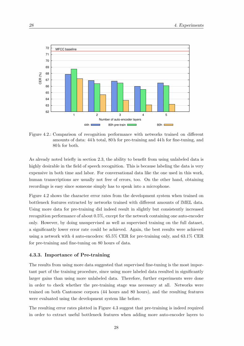
44h 80h pre-train 80h

Figure 4.2.: Comparison of recognition performance with networks trained on di↵erentamounts of data: 44 h total, 80 h for pre-training and 44 h for fine-tuning, and80 h for both.

As already noted briefly in section 2.3, the ability to benefit from using unlabeled data is

highly desirable in the field of speech recognition. This is because labeling the data is very

expensive in both time and labor. For conversational data like the one used in this work,

human transcriptions are usually not free of errors, too. On the other hand, obtaining

recordings is easy since someone simply has to speak into a microphone.

Figure 4.2 shows the character error rates from the development system when trained on

bottleneck features extracted by networks trained with di↵erent amounts of lMEL data.

Using more data for pre-training did indeed result in slightly but consistently increased

recognition performance of about 0.5%, except for the network containing one auto-encoder

only. However, by doing unsupervised as well as supervised training on the full dataset,

a significantly lower error rate could be achieved. Again, the best results were achieved

using a network with 4 auto-encoders: 65.5% CER for pre-training only, and 63.1% CER

for pre-training and fine-tuning on 80 hours of data.

4.3.3. Importance of Pre-training

The results from using more data suggested that supervised fine-tuning is the most impor-

tant part of the training procedure, since using more labeled data resulted in significantly

larger gains than using more unlabeled data. Therefore, further experiments were done

in order to check whether the pre-training stage was necessary at all. Networks were

trained on both Cantonese corpora (44 hours and 80 hours), and the resulting features

were evaluated using the development system like before.

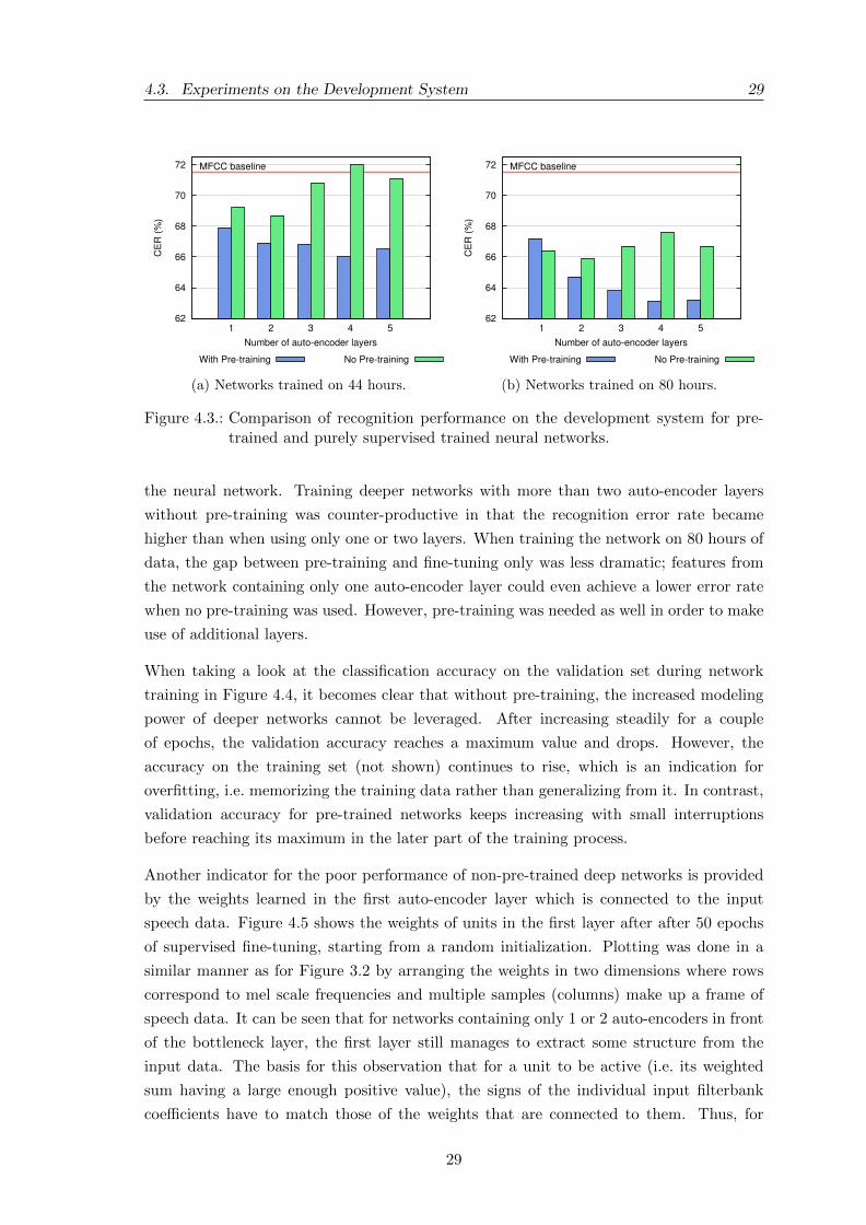
The resulting error rates plotted in Figure 4.3 suggest that pre-training is indeed required

in order to extract useful bottleneck features when adding more auto-encoder layers to

28

4.3. Experiments on the Development System 29

62

64

66

68

70

72

1 2 3 4 5

CE

R (

%)


MFCC baseline

With Pre-training No Pre-training

(a) Networks trained on 44 hours.

62

64

66

68

70

72

1 2 3 4 5

CE

R (

%)


MFCC baseline

With Pre-training No Pre-training

(b) Networks trained on 80 hours.

Figure 4.3.: Comparison of recognition performance on the development system for pre-trained and purely supervised trained neural networks.

the neural network. Training deeper networks with more than two auto-encoder layers

without pre-training was counter-productive in that the recognition error rate became

higher than when using only one or two layers. When training the network on 80 hours of

data, the gap between pre-training and fine-tuning only was less dramatic; features from

the network containing only one auto-encoder layer could even achieve a lower error rate

when no pre-training was used. However, pre-training was needed as well in order to make

use of additional layers.

When taking a look at the classification accuracy on the validation set during network

training in Figure 4.4, it becomes clear that without pre-training, the increased modeling

power of deeper networks cannot be leveraged. After increasing steadily for a couple

of epochs, the validation accuracy reaches a maximum value and drops. However, the

accuracy on the training set (not shown) continues to rise, which is an indication for

overfitting, i.e. memorizing the training data rather than generalizing from it. In contrast,

validation accuracy for pre-trained networks keeps increasing with small interruptions

before reaching its maximum in the later part of the training process.

Another indicator for the poor performance of non-pre-trained deep networks is provided

by the weights learned in the first auto-encoder layer which is connected to the input

speech data. Figure 4.5 shows the weights of units in the first layer after after 50 epochs

of supervised fine-tuning, starting from a random initialization. Plotting was done in a

similar manner as for Figure 3.2 by arranging the weights in two dimensions where rows

correspond to mel scale frequencies and multiple samples (columns) make up a frame of

speech data. It can be seen that for networks containing only 1 or 2 auto-encoders in front

of the bottleneck layer, the first layer still manages to extract some structure from the

input data. The basis for this observation that for a unit to be active (i.e. its weighted

sum having a large enough positive value), the signs of the individual input filterbank

coe�cients have to match those of the weights that are connected to them. Thus, for

29

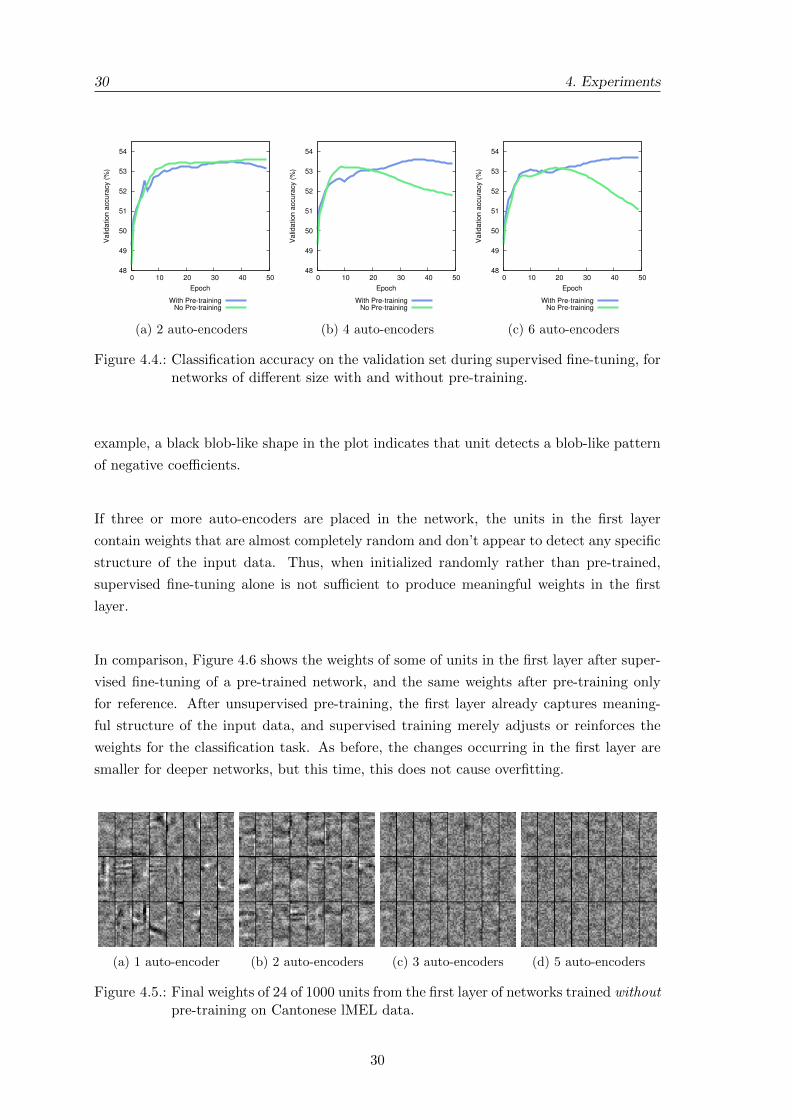
30 4. Experiments

48

49

50

51

52

53

54

0 10 20 30 40 50

Va

lida

tion

acc

ura

cy (

%)

Epoch

With Pre-trainingNo Pre-training

(a) 2 auto-encoders

48

49

50

51

52

53

54

0 10 20 30 40 50

Va

lida

tion

acc

ura

cy (

%)

Epoch


(b) 4 auto-encoders

48

49

50

51

52

53

54

0 10 20 30 40 50

Va

lida

tion

acc

ura

cy (

%)

Epoch


(c) 6 auto-encoders

Figure 4.4.: Classification accuracy on the validation set during supervised fine-tuning, fornetworks of di↵erent size with and without pre-training.

example, a black blob-like shape in the plot indicates that unit detects a blob-like pattern

of negative coe�cients.

If three or more auto-encoders are placed in the network, the units in the first layer

contain weights that are almost completely random and don’t appear to detect any specific

structure of the input data. Thus, when initialized randomly rather than pre-trained,

supervised fine-tuning alone is not su�cient to produce meaningful weights in the first

layer.

In comparison, Figure 4.6 shows the weights of some of units in the first layer after super-

vised fine-tuning of a pre-trained network, and the same weights after pre-training only

for reference. After unsupervised pre-training, the first layer already captures meaning-

ful structure of the input data, and supervised training merely adjusts or reinforces the

weights for the classification task. As before, the changes occurring in the first layer are

smaller for deeper networks, but this time, this does not cause overfitting.

(a) 1 auto-encoder (b) 2 auto-encoders (c) 3 auto-encoders (d) 5 auto-encoders

Figure 4.5.: Final weights of 24 of 1000 units from the first layer of networks trained without

pre-training on Cantonese lMEL data.

30

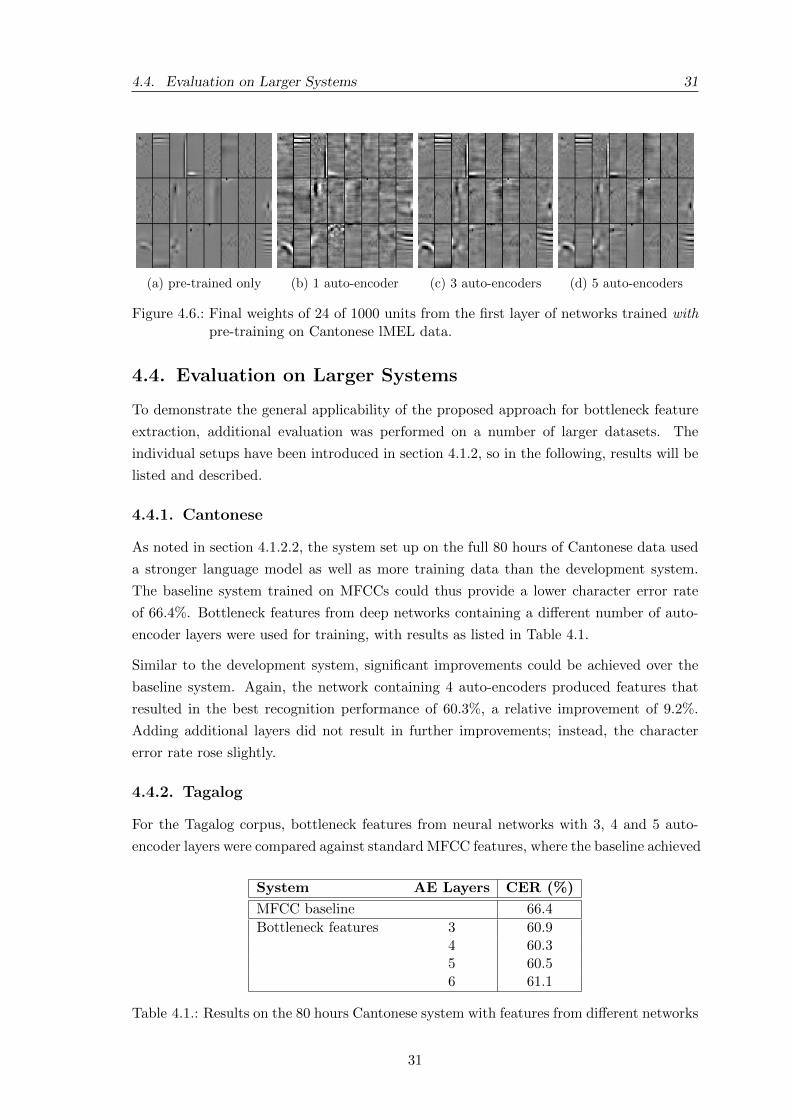
4.4. Evaluation on Larger Systems 31

(a) pre-trained only (b) 1 auto-encoder (c) 3 auto-encoders (d) 5 auto-encoders

Figure 4.6.: Final weights of 24 of 1000 units from the first layer of networks trained with

pre-training on Cantonese lMEL data.

4.4. Evaluation on Larger Systems

To demonstrate the general applicability of the proposed approach for bottleneck feature

extraction, additional evaluation was performed on a number of larger datasets. The

individual setups have been introduced in section 4.1.2, so in the following, results will be

listed and described.

4.4.1. Cantonese

As noted in section 4.1.2.2, the system set up on the full 80 hours of Cantonese data used

a stronger language model as well as more training data than the development system.

The baseline system trained on MFCCs could thus provide a lower character error rate

of 66.4%. Bottleneck features from deep networks containing a di↵erent number of auto-

encoder layers were used for training, with results as listed in Table 4.1.

Similar to the development system, significant improvements could be achieved over the

baseline system. Again, the network containing 4 auto-encoders produced features that

resulted in the best recognition performance of 60.3%, a relative improvement of 9.2%.

Adding additional layers did not result in further improvements; instead, the character

error rate rose slightly.

4.4.2. Tagalog

For the Tagalog corpus, bottleneck features from neural networks with 3, 4 and 5 auto-

encoder layers were compared against standard MFCC features, where the baseline achieved

System AE Layers CER (%)

MFCC baseline 66.4Bottleneck features 3 60.9

4 60.35 60.56 61.1

Table 4.1.: Results on the 80 hours Cantonese system with features from di↵erent networks

31

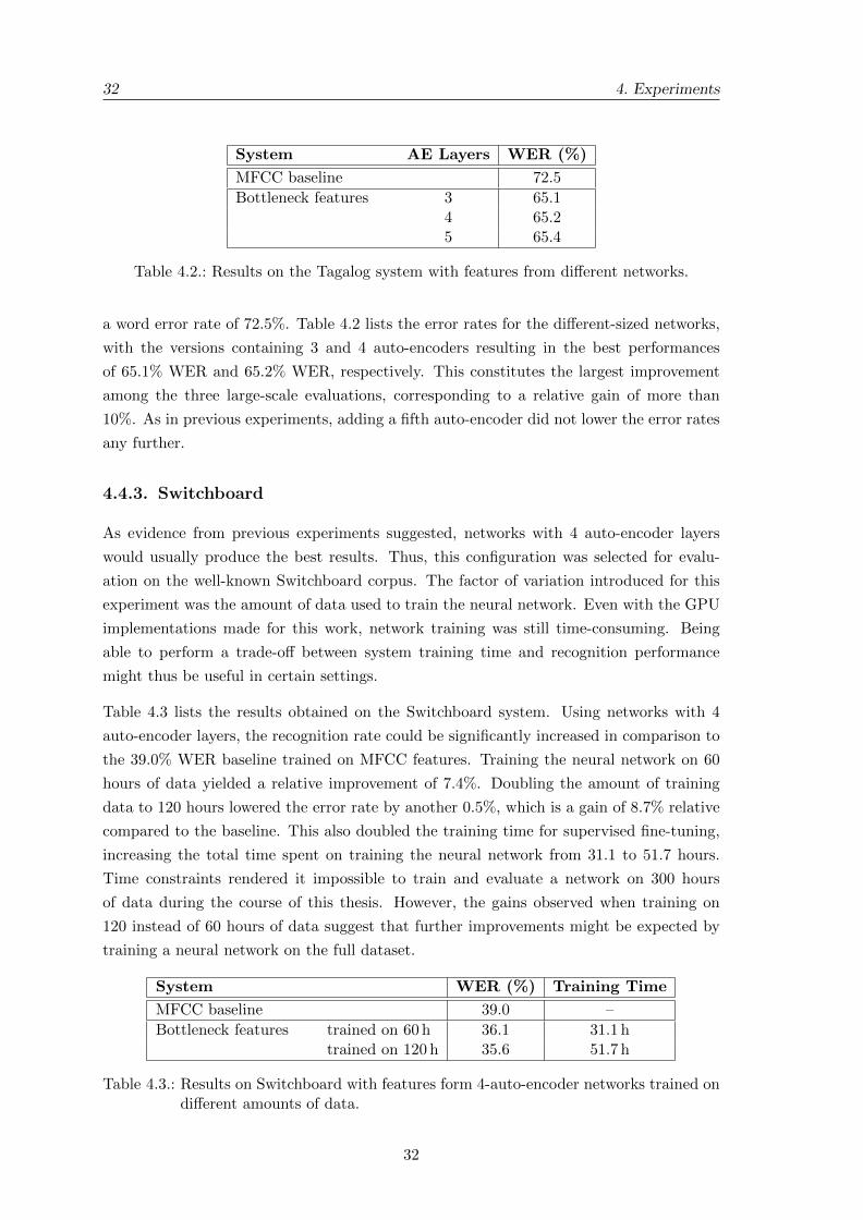
32 4. Experiments

System AE Layers WER (%)

MFCC baseline 72.5Bottleneck features 3 65.1

4 65.25 65.4

Table 4.2.: Results on the Tagalog system with features from di↵erent networks.

a word error rate of 72.5%. Table 4.2 lists the error rates for the di↵erent-sized networks,

with the versions containing 3 and 4 auto-encoders resulting in the best performances

of 65.1% WER and 65.2% WER, respectively. This constitutes the largest improvement

among the three large-scale evaluations, corresponding to a relative gain of more than

10%. As in previous experiments, adding a fifth auto-encoder did not lower the error rates

any further.

4.4.3. Switchboard

As evidence from previous experiments suggested, networks with 4 auto-encoder layers

would usually produce the best results. Thus, this configuration was selected for evalu-

ation on the well-known Switchboard corpus. The factor of variation introduced for this

experiment was the amount of data used to train the neural network. Even with the GPU

implementations made for this work, network training was still time-consuming. Being

able to perform a trade-o↵ between system training time and recognition performance

might thus be useful in certain settings.

Table 4.3 lists the results obtained on the Switchboard system. Using networks with 4

auto-encoder layers, the recognition rate could be significantly increased in comparison to

the 39.0% WER baseline trained on MFCC features. Training the neural network on 60

hours of data yielded a relative improvement of 7.4%. Doubling the amount of training

data to 120 hours lowered the error rate by another 0.5%, which is a gain of 8.7% relative

compared to the baseline. This also doubled the training time for supervised fine-tuning,

increasing the total time spent on training the neural network from 31.1 to 51.7 hours.

Time constraints rendered it impossible to train and evaluate a network on 300 hours

of data during the course of this thesis. However, the gains observed when training on

120 instead of 60 hours of data suggest that further improvements might be expected by

training a neural network on the full dataset.

System WER (%) Training Time

MFCC baseline 39.0 –Bottleneck features trained on 60 h 36.1 31.1 h

trained on 120 h 35.6 51.7 h

Table 4.3.: Results on Switchboard with features form 4-auto-encoder networks trained ondi↵erent amounts of data.

32

4.4. Evaluation on Larger Systems 33

The training times listed in Table 4.3 were obtained by training the networks on a NVIDIA

GTX 480 graphics processor, which contains 480 cores running at 700 MHz. For more

details regarding the training of neural networks on GPUs, please refer to the respective

appendix B.

33

Conclusion

5.1. Summary

In this work, a new approach for training deep neural networks used for the extraction of

bottleneck features has been proposed. In contrast to earlier work regarding bottleneck

features, the new network architecture is able to e↵ectively make use of the increased model

capacity of deep neural networks by producing features that increase the final recognition

accuracy. The techniques presented resulted in significant and consistent improvements

over standard MFCC-based systems on datasets in three di↵erent languages. The relative

improvements in terms of character or word error rate, respectively, were 9.2% CER for

Cantonese, 10.3% WER for Tagalog and 8.7% WER on the Switchboard task.

It has been demonstrated that with the proposed architecture, deep neural networks with

many layers are able to outperform shallow networks by extracting more useful bottleneck

features. However, this ability depends on a suitable training algorithm, and the greedy,

layer-wise and unsupervised pre-training strategy popular in deep learning was able to

produce models with superior performance. Closer examination of the network learning

procedure and the learned weight parameters suggested that without pre-training, deep

neural networks tend to overfit and their first layer fails to extract meaningful structure

from the training data.

Experiments showed that extracting bottleneck features from log mel scale filterbank co-

e�cients results in better recognition performance compared to features extracted from

MFCCs. Further small improvements could be achieved by using more, unlabeled data

when pre-training individual layers.

Finally, denoising auto-encoders proved to be robust models for building deep networks and

initializing bottleneck networks. Training the models was straightforward and fast, and the

performance improvements obtained were equally encouraging than the results reported

34

5.2. Discussion 35

in previous works regarding bottleneck features and hybrid systems, which mostly relied

on restricted Boltzmann machines for pre-training.

5.2. Discussion

In this thesis, multiple experiments have been performed in order to better understand the

influence of neural network topology and input data. For the latter, it could be shown that

training the network on log mel scale filterbank coe�cients resulted in better recognition

performance than training on MFCC frames (see section 4.3.1). This is consistent with

findings in by Mohamed et al. regarding restricted Boltzmann machines [MHP12]. In

order to actually confirm this for denoising auto-encoders as used in this work, further

experiments might need to be performed to rule out the possibility that the performance

gains were simply due to the log mel scale features having a higher dimensionality (in this

case, 330 compared to of 143 MFCC elements for a single feature vector). This could be

done by either reducing the number of mel coe�cients or increasing the number of MFCCs

used.

In terms of network topology, it could be shown that features extracted from networks with

more hidden layers resulted in higher recognition accuracy. This is expected when using a

suitable learning algorithm, as increasing the modeling power of the neural network should

result in more useful bottleneck features. However, when adding more then 4 auto-encoder

layers, no further improvements in terms of recognition rate could be observed. Possible

reasons for this include not having enough data available for training networks with such

a large number of parameters, or that the denoising auto-encoders in higher levels did not

extract very useful features during pre-training.

As described in section 4.3.3, pre-training turned out to be important for extracting use-

ful features with deep neural networks. The gap between recognition rates on features

extracted with and without pre-training was less extreme when training the networks on

80 instead of 44 hours. Similar findings have been reported by Seide et al., who noted

that in their best configuration regarding a hybrid DNN/HMM setup trained 300 hours,

pre-training produced only small gains over networks that were trained in a purely su-

pervised fashion [SLY11]. This suggests that while being generally helpful, unsupervised

pre-training might be especially crucial if only little training data is available. Another

indicator for this correlation is that while yielding small gains, adding more data for pre-

training is not as beneficial as fine-tuning on more data as shown in section 4.3.2.

5.3. Outlook

The recognition setups used in this thesis employed relatively simple algorithms for acous-

tic modeling and language modeling. Therefore, additional evaluation needs to be done

in heavily tuned systems that use discriminative training, speaker adaption and strong

35

36 5. Conclusion

language models, with the hope that the relative gains achieved (9% to 10% relative) will

persist. The same is true for systems build on very large corpora that consist of thousands

of hours of speech data.

Amongst further experiments are the ones that address the open questions formulated

above, for example what constitutes the best input data to extract features from. Apart

from that, the network architecture and training procedures proposed provide a solid foun-

dation for further enhancements. It might be interesting to fully evaluate other methods

for pre-training the individual layers, with possible candidates being mean-covariance re-

stricted Boltzmann machines [DRMH10] and contractive auto-encoders [RVM+11].

The fine-tuning step could be optimized as well by training the neural network to es-

timate context-dependent instead of context-independent states, which was reported to

improve the resulting features in previous works [YS11], [SKR12]. Furthermore, it might

be worthwhile to apply the recently proposed “dropout” training procedure, in which hid-

den units are randomly omitted from the network in order to prevent overfitting caused

by co-adaptation of neurons [HSK+12].

36

Bibliography

[AHMJP12] O. Abdel-Hamid, A. Mohamed, H. Jiang, and G. Penn, “Applying convolu-

tional neural networks concepts to hybrid NN-HMM model for speech recog-

nition,” in Acoustics, Speech and Signal Processing (ICASSP), 2012 IEEE

International Conference on. IEEE, 2012, pp. 4277–4280.

[AHS85] D. Ackley, G. Hinton, and T. Sejnowski, “A learning algorithm for boltzmann

machines,”Cognitive science, vol. 9, no. 1, pp. 147–169, 1985.

[BBB+10] J. Bergstra, O. Breuleux, F. Bastien, P. Lamblin, R. Pascanu, G. Desjardins,

J. Turian, D. Warde-Farley, and Y. Bengio, “Theano: a CPU and GPU Math

Expression Compiler,” in Proceedings of the Python for Scientific Computing

Conference (SciPy), Jun. 2010, Oral Presentation.

[Ben09] Y. Bengio, “Learning deep architectures for AI,” Foundations and Trends in

Machine Learning, vol. 2, no. 1, pp. 1–127, 2009.

[BLPL07] Y. Bengio, P. Lamblin, D. Popovici, and H. Larochelle, “Greedy layer-wise

training of deep networks,” Advances in neural information processing sys-

tems, vol. 19, p. 153, 2007.

[BM94] H. Bourlard and N. Morgan, Connectionist speech recognition: a hybrid ap-

proach. Springer, 1994, vol. 247.

[DGB11] Y. Dauphin, X. Glorot, and Y. Bengio, “Large-scale learning of embeddings

with reconstruction sampling,” in Proceedings of the Twenty-eighth Interna-

tional Conference on Machine Learning (ICML’11), 2011.

[DM80] S. Davis and P. Mermelstein, “Comparison of parametric representations for

monosyllabic word recognition in continuously spoken sentences,” Acoustics,

Speech and Signal Processing, IEEE Transactions on, vol. 28, no. 4, pp. 357–

366, 1980.

[DRMH10] G. Dahl, M. Ranzato, A. Mohamed, and G. Hinton, “Phone recognition with

the mean-covariance restricted boltzmann machine,” Advances in neural in-

formation processing systems, vol. 23, pp. 469–477, 2010.

[DYDA12] G. Dahl, D. Yu, L. Deng, and A. Acero, “Context-Dependent Pre-Trained

Deep Neural Networks for Large-Vocabulary Speech Recognition,” Audio,

37

38 Bibliography

Speech, and Language Processing, IEEE Transactions on, vol. 20, no. 1, pp.

30–42, 2012.

[EZ88] J. Elman and D. Zipser, “Learning the hidden structure of speech,”The Jour-

nal of the Acoustical Society of America, vol. 83, p. 1615, 1988.

[FGH+97] M. Finke, P. Geutner, H. Hild, T. Kemp, K. Ries, and M. Westphal, “The

Karlsruhe-Verbmobil speech recognition engine,” in Acoustics, Speech, and

Signal Processing, 1997. ICASSP-97., 1997 IEEE International Conference

on, vol. 1. IEEE, 1997, pp. 83–86.

[FRB97] V. Fontaine, C. Ris, and J. Boite, “Nonlinear discriminant analysis for im-

proved speech recognition,” in Proc. Eurospeech, vol. 97, 1997, pp. 2071–2074.

[GB10] X. Glorot and Y. Bengio, “Understanding the di�culty of training deep feed-

forward neural networks,” in Proceedings of the International Conference on

Artificial Intelligence and Statistics (AISTATS’10). Society for Artificial In-

telligence and Statistics, 2010.

[GBB11] X. Glorot, A. Bordes, and Y. Bengio, “Domain adaptation for large-scale

sentiment classification: A deep learning approach,” in Proceedings of the

Twenty-eight International Conference on Machine Learning, ICML, 2011.

[GHM92] J. Godfrey, E. Holliman, and J. McDaniel, “SWITCHBOARD: Telephone

speech corpus for research and development,” in Acoustics, Speech, and Sig-

nal Processing, 1992. ICASSP-92., 1992 IEEE International Conference on,

vol. 1. IEEE, 1992, pp. 517–520.

[GKKC07] F. Grezl, M. Karafiat, S. Kontar, and J. Cernocky, “Probabilistic and Bottle-

Neck Features for LVCSR of Meetings,” in Acoustics, Speech and Signal Pro-

cessing, 2007. ICASSP 2007. IEEE International Conference on, vol. 4, april

2007, pp. IV–757 –IV–760.

[HDY+12] G. Hinton, L. Deng, D. Yu, G. Dahl, A. Mohamed, N. Jaitly, A. Senior,

V. Vanhoucke, P. Nguyen, T. Sainath et al., “Deep neural networks for acous-

tic modeling in speech recognition,” IEEE Signal Processing Magazine, 2012.

[HES00] H. Hermansky, D. Ellis, and S. Sharma, “Tandem connectionist feature ex-

traction for conventional HMM systems,” in Acoustics, Speech, and Signal

Processing, 2000. ICASSP’00. Proceedings. 2000 IEEE International Con-

ference on, vol. 3. IEEE, 2000, pp. 1635–1638.

[Hin89] G. Hinton,“Connectionist learning procedures,”Artificial intelligence, vol. 40,

no. 1, pp. 185–234, 1989.

[Hin10] ——, “A practical guide to training restricted boltzmann machines,”Momen-

tum, vol. 9, p. 1, 2010.

38

Bibliography 39

[HOT06] G. Hinton, S. Osindero, and Y. Teh, “A fast learning algorithm for deep belief

nets,”Neural computation, vol. 18, no. 7, pp. 1527–1554, 2006.

[HSK+12] G. Hinton, N. Srivastava, A. Krizhevsky, I. Sutskever, and R. Salakhutdinov,

“Improving neural networks by preventing co-adaptation of feature detectors,”

arXiv preprint arXiv:1207.0580, 2012.

[IAR] “IARPA-BAA-11-02,” http://www.iarpa.gov/Programs/ia/Babel/babel.

html, IARPA.

[J+04] D. Johnson et al., “ICSI Quicknet software package,” http://www.icsi.

berkeley.edu/Speech/qn.html, 2004.

[JNSV12] N. Jaitly, P. Nguyen, A. Senior, and V. Vanhoucke, “An application of

pretrained deep neural networks to large vocabulary conversational speech

recognition,”Tech. Rep. 001, Department of Computer Science, University of

Toronto, Tech. Rep., 2012.

[KSH12] A. Krizhevsky, I. Sutskever, and G. Hinton,“Imagenet classification with deep

convolutional neural networks,” Advances in Neural Information Processing

Systems, vol. 25, 2012.

[LB95] Y. LeCun and Y. Bengio, “Convolutional networks for images, speech, and

time series,” The handbook of brain theory and neural networks, vol. 3361,

1995.

[LGRN09] H. Lee, R. Grosse, R. Ranganath, and A. Ng, “Convolutional deep belief net-

works for scalable unsupervised learning of hierarchical representations,” in

Proceedings of the 26th Annual International Conference on Machine Learn-

ing. ACM, 2009, pp. 609–616.

[Lip89] R. Lippmann, “Review of neural networks for speech recognition,” Neural

computation, vol. 1, no. 1, pp. 1–38, 1989.

[LMD+11] Q. Le, R. Monga, M. Devin, G. Corrado, K. Chen, M. Ranzato, J. Dean, and

A. Ng, “Building high-level features using large scale unsupervised learning,”

arXiv preprint arXiv:1112.6209, 2011.

[MDH09] A. Mohamed, G. Dahl, and G. Hinton, “Deep belief networks for phone recog-

nition,” in NIPS Workshop on Deep Learning for Speech Recognition and Re-

lated Applications, 2009.

[MHP12] A. Mohamed, G. Hinton, and G. Penn, “Understanding how deep belief net-

works perform acoustic modelling,” in Acoustics, Speech and Signal Process-

ing (ICASSP), 2012 IEEE International Conference on. IEEE, 2012, pp.

4273–4276.

39

http://www.iarpa.gov/Programs/ia/Babel/babel.html

http://www.iarpa.gov/Programs/ia/Babel/babel.html

http://www.icsi.berkeley.edu/Speech/qn.html

http://www.icsi.berkeley.edu/Speech/qn.html

40 Bibliography

[MKC+11] L. Mangu, H. Kuo, S. Chu, B. Kingsbury, G. Saon, H. Soltau, and F. Biadsy,

“The IBM 2011 GALE Arabic speech transcription system,” in Automatic

Speech Recognition and Understanding (ASRU), 2011 IEEE Workshop on.

IEEE, 2011, pp. 272–277.

[MRBL07] Y. Marc’Aurelio Ranzato, L. Boureau, and Y. LeCun,“Sparse feature learning

for deep belief networks,”Advances in neural information processing systems,

vol. 20, pp. 1185–1192, 2007.

[MRCL06] C. Marc’Aurelio Ranzato, S. Chopra, and Y. LeCun, “E�cient learning of

sparse representations with an energy-based model,” Advances in neural in-

formation processing systems, vol. 19, pp. 1137–1144, 2006.

[PNH86] D. C. Plaut, S. J. Nowlan, and G. E. Hinton, “Experiments on learning by

back propagation,” Carnegie Mellon University, Tech. Rep., 1986.

[RHW86] D. Rumelhart, G. Hintont, and R. Williams, “Learning representations by

back-propagating errors,”Nature, vol. 323, no. 6088, pp. 533–536, 1986.

[Ros58] F. Rosenblatt, “The perceptron: a probabilistic model for information storage

and organization in the brain.” Psychological review, vol. 65, no. 6, p. 386,

1958.

[RVM+11] S. Rifai, P. Vincent, X. Muller, X. Glorot, and Y. Bengio, “Contractive auto-

encoders: Explicit invariance during feature extraction,” in Proceedings of

the Twenty-eight International Conference on Machine Learning (ICML’11),

2011.

[SD91] J. Sietsma and R. Dow, “Creating artificial neural networks that generalize,”

Neural Networks, vol. 4, no. 1, pp. 67–79, 1991.

[SKK+07] T. Serre, G. Kreiman, M. Kouh, C. Cadieu, U. Knoblich, and T. Poggio,

“A quantitative theory of immediate visual recognition,” Progress in Brain

Research, vol. 165, pp. 33–56, 2007.

[SKR12] T. Sainath, B. Kingsbury, and B. Ramabhadran, “Auto-encoder bottleneck

features using deep belief networks,” in Acoustics, Speech and Signal Process-

ing (ICASSP), 2012 IEEE International Conference on. IEEE, 2012, pp.

4153–4156.

[SLY11] F. Seide, G. Li, and D. Yu, “Conversational speech transcription using

context-dependent deep neural networks,” in Proc. Interspeech, 2011, pp. 437–

440.

[SMFW01] H. Soltau, F. Metze, C. Fugen, and A. Waibel, “A one-pass decoder based on

polymorphic linguistic context assignment,” in Automatic Speech Recognition

and Understanding, 2001. ASRU’01. IEEE Workshop on. IEEE, 2001, pp.

214–217.

40

Bibliography 41

[VLBM08] P. Vincent, H. Larochelle, Y. Bengio, and P. Manzagol, “Extracting and com-

posing robust features with denoising autoencoders,” in Proceedings of the

25th international conference on Machine learning. ACM, 2008, pp. 1096–

1103.

[VLL+10] P. Vincent, H. Larochelle, I. Lajoie, Y. Bengio, and P. Manzagol, “Stacked

denoising autoencoders: Learning useful representations in a deep network

with a local denoising criterion,”The Journal of Machine Learning Research,

vol. 11, pp. 3371–3408, 2010.

[WHH+89] A. Waibel, T. Hanazawa, G. Hinton, K. Shikano, and K. Lang, “Phoneme

recognition using time-delay neural networks,” Acoustics, Speech and Signal

Processing, IEEE Transactions on, vol. 37, no. 3, pp. 328–339, 1989.

[WS87] R. Watrous and L. Shastri, “Learning phonetic features using connectionist

networks,”The Journal of the Acoustical Society of America, vol. 81, no. S1,

pp. S93–S94, 1987.

[WSS89] A. Waibel, H. Sawai, and K. Shikano, “Modularity and scaling in large phone-

mic neural networks,”Acoustics, Speech and Signal Processing, IEEE Trans-

actions on, vol. 37, no. 12, pp. 1888–1898, 1989.

[YS11] D. Yu and M. Seltzer, “Improved bottleneck features using pretrained deep

neural networks,” Proc. Interspeech 2011, pp. 237–240, 2011.

41

Appendix

A. Training Algorithms

In this thesis, backpropagation and gradient descent have been used to train neural net-

works to minimizing an error term (see section 2.2). Backpropagation enables the prop-

agation of the output error through the network so that each unit gets an error signal

corresponding to its contribution to the total error. The gradient of the error signal is

then used to update the individual weight and bias values.

A.1. Denoising Auto-encoder

The denoising auto-encoders used in this work performed both encoding and decoding

using the same weight parameters (“tied” weights). Thus, the computations described in

section 2.3.2.2 can be expanded as follows:

z = �z

�W

Ty + c

�(A.1)

= �z

�W

T�y (Wx+ b) + c

�(A.2)

Here, x constitutes the corrupted version of the auto-encoder input x, z is the reconstruc-

tion and W is the weight matrix. �y and �z are the activation functions for the hidden

and output layer, and b and c define the bias values of the hidden and output units,

respectively.

For the first auto-encoder layer, the input is given by a frame of real-valued coe�cients

extracted from speech data, so the mean squared error term was used for training. In

vector notation, this term can be formulated as

E (x, z)2 =1

2(x� z)2 (A.3)

In order to compute the updates for the weight matrix �W , the error term has to be

propagated backwards through the network, starting with the output units. The mean

squared error is straightforward to di↵erentiate, and the derivative of the hyperbolic tan-

gent used for �z(x) is given by (1 � x

2). With az = W

Ty + c, the error for the output

units is given by:

�z = � (x� z)�1� a

2z

�(A.4)

43

44 Appendix

Using the backpropagation algorithm and abbreviating the activation of the hidden units

with ay = Wx+ b, the error term for the hidden layer is given by

�y =⇣W

TT

�z

⌘�

0y (ay) (A.5)

Di↵erentiating the sigmoid function yields x · (1� x), so this equals to

�y = (W �z)ay (1� ay) (A.6)

In a fully connected network, the derivatives with respect to the weights are computed

by multiplying the error of a layer with its input values [RHW86]. Since the same weight

matrix is used to compute y and the reconstruction z, the actual derivative for updating

the weights is given by the sum of the error terms in Eq. A.4 and Eq. A.6, each multiplied

with the respective input values:

@E

@W

= �yxT + �zy

T (A.7)

= (W �z)ay (1� ay) xT +

�� (x� z)

�1� a

2z

�y

T�

(A.8)

In this work, standard gradient descent was used for training denoising auto-encoders.

Thus, weights are updated by subtracting a fraction of the respective derivative as deter-

mined by the learning rate ⌘:

�W = �⌘

@E

@W

(A.9)

The hidden and visible bias parameters are updated in a similar manner, with the di↵erence

that the propagated error terms are not being multiplied by the input of the layer:

�b = �⌘�y �c = �⌘�z (A.10)

In auto-encoders that did not model the input data directly, a cross-entropy error term

and a sigmoid activation function for the output units was being used. For this case, the

weight updates can be computed in the same way as before. The error term for y stays

the same, but the other ones have to be changed accordingly

E (x, z)H = x log z + (1� x) log z (A.11)

�z = x� z (A.12)

@E

@W

= (W �z)ay (1� ay) xT + (x� z)yT (A.13)

A.2. Multi-layer Perceptron

After pre-training, the stack of auto-encoder layers was transformed into a standard multi-

layer perceptron, and additional layers were being added on top of it. In order to perform

44

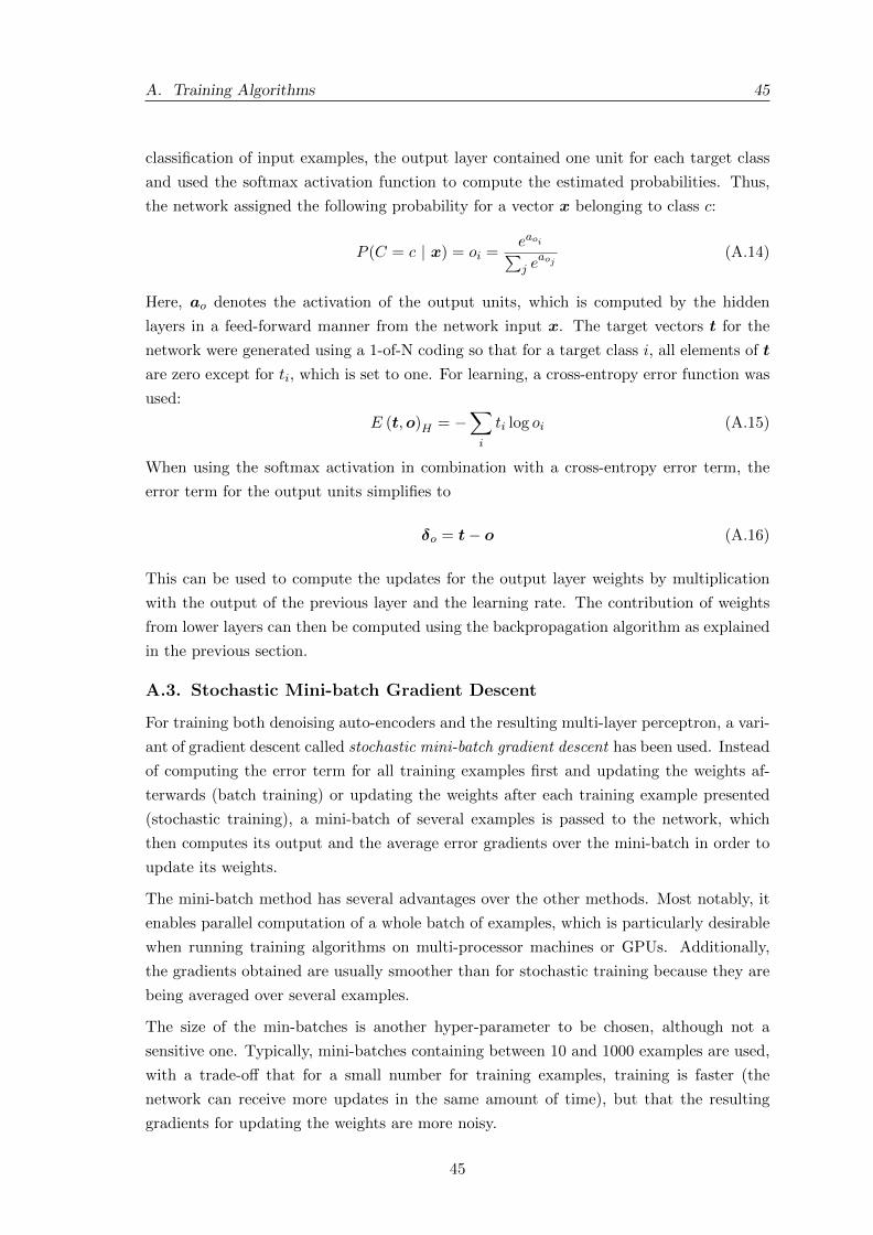
A. Training Algorithms 45

classification of input examples, the output layer contained one unit for each target class

and used the softmax activation function to compute the estimated probabilities. Thus,

the network assigned the following probability for a vector x belonging to class c:

P (C = c | x) = oi =e

ao

i

Pj e

ao

j

(A.14)

Here, ao denotes the activation of the output units, which is computed by the hidden

layers in a feed-forward manner from the network input x. The target vectors t for the

network were generated using a 1-of-N coding so that for a target class i, all elements of t

are zero except for ti, which is set to one. For learning, a cross-entropy error function was

used:

E (t,o)H = �X

i

ti log oi (A.15)

When using the softmax activation in combination with a cross-entropy error term, the

error term for the output units simplifies to

�o = t� o (A.16)

This can be used to compute the updates for the output layer weights by multiplication

with the output of the previous layer and the learning rate. The contribution of weights

from lower layers can then be computed using the backpropagation algorithm as explained

in the previous section.

A.3. Stochastic Mini-batch Gradient Descent

For training both denoising auto-encoders and the resulting multi-layer perceptron, a vari-

ant of gradient descent called stochastic mini-batch gradient descent has been used. Instead

of computing the error term for all training examples first and updating the weights af-

terwards (batch training) or updating the weights after each training example presented

(stochastic training), a mini-batch of several examples is passed to the network, which

then computes its output and the average error gradients over the mini-batch in order to

update its weights.

The mini-batch method has several advantages over the other methods. Most notably, it

enables parallel computation of a whole batch of examples, which is particularly desirable

when running training algorithms on multi-processor machines or GPUs. Additionally,

the gradients obtained are usually smoother than for stochastic training because they are

being averaged over several examples.

The size of the min-batches is another hyper-parameter to be chosen, although not a

sensitive one. Typically, mini-batches containing between 10 and 1000 examples are used,

with a trade-o↵ that for a small number for training examples, training is faster (the

network can receive more updates in the same amount of time), but that the resulting

gradients for updating the weights are more noisy.

45

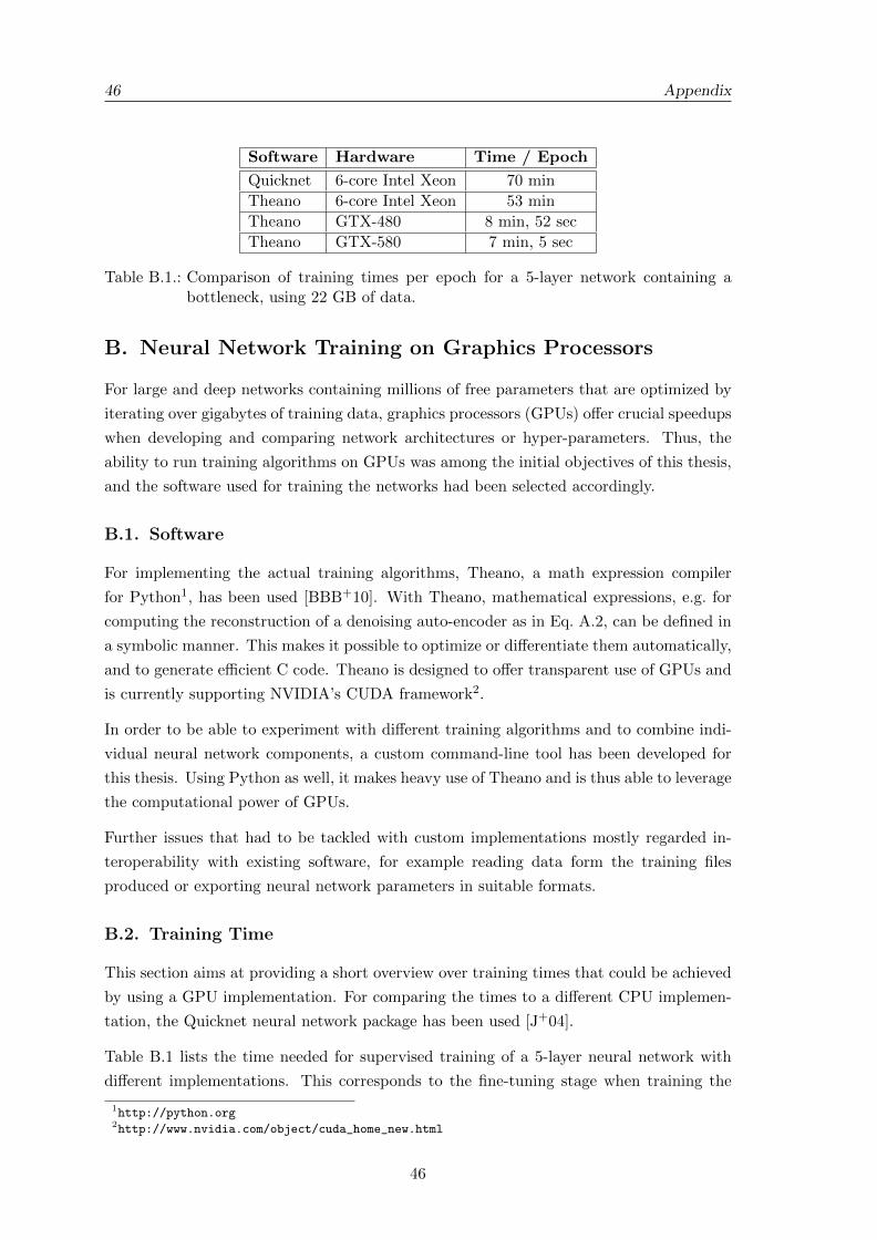
46 Appendix

Software Hardware Time / Epoch

Quicknet 6-core Intel Xeon 70 minTheano 6-core Intel Xeon 53 minTheano GTX-480 8 min, 52 secTheano GTX-580 7 min, 5 sec

Table B.1.: Comparison of training times per epoch for a 5-layer network containing abottleneck, using 22 GB of data.

B. Neural Network Training on Graphics Processors

For large and deep networks containing millions of free parameters that are optimized by

iterating over gigabytes of training data, graphics processors (GPUs) o↵er crucial speedups

when developing and comparing network architectures or hyper-parameters. Thus, the

ability to run training algorithms on GPUs was among the initial objectives of this thesis,

and the software used for training the networks had been selected accordingly.

B.1. Software

For implementing the actual training algorithms, Theano, a math expression compiler

for Python1, has been used [BBB+10]. With Theano, mathematical expressions, e.g. for

computing the reconstruction of a denoising auto-encoder as in Eq. A.2, can be defined in

a symbolic manner. This makes it possible to optimize or di↵erentiate them automatically,

and to generate e�cient C code. Theano is designed to o↵er transparent use of GPUs and

is currently supporting NVIDIA’s CUDA framework2.

In order to be able to experiment with di↵erent training algorithms and to combine indi-

vidual neural network components, a custom command-line tool has been developed for

this thesis. Using Python as well, it makes heavy use of Theano and is thus able to leverage

the computational power of GPUs.

Further issues that had to be tackled with custom implementations mostly regarded in-

teroperability with existing software, for example reading data form the training files

produced or exporting neural network parameters in suitable formats.

B.2. Training Time

This section aims at providing a short overview over training times that could be achieved

by using a GPU implementation. For comparing the times to a di↵erent CPU implemen-

tation, the Quicknet neural network package has been used [J+04].

Table B.1 lists the time needed for supervised training of a 5-layer neural network with

di↵erent implementations. This corresponds to the fine-tuning stage when training the

1http://python.org

2http://www.nvidia.com/object/cuda_home_new.html

46

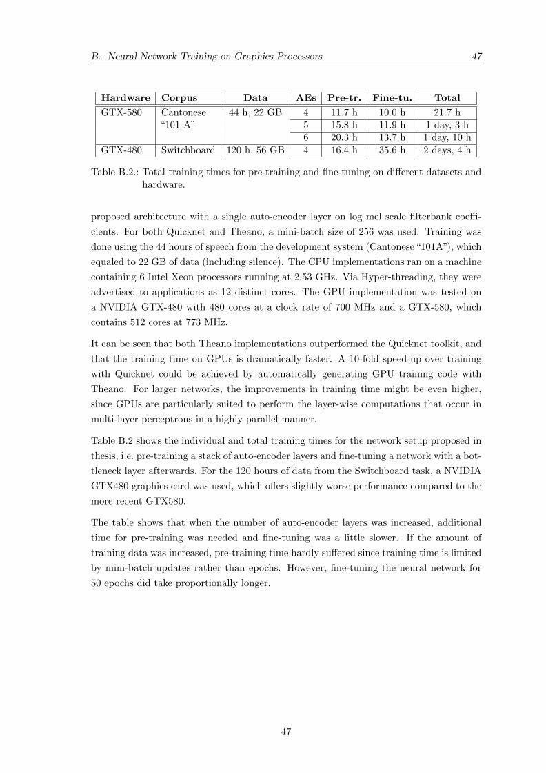
B. Neural Network Training on Graphics Processors 47

Hardware Corpus Data AEs Pre-tr. Fine-tu. Total

GTX-580 Cantonese 44 h, 22 GB 4 11.7 h 10.0 h 21.7 h“101 A” 5 15.8 h 11.9 h 1 day, 3 h

6 20.3 h 13.7 h 1 day, 10 hGTX-480 Switchboard 120 h, 56 GB 4 16.4 h 35.6 h 2 days, 4 h

Table B.2.: Total training times for pre-training and fine-tuning on di↵erent datasets andhardware.

proposed architecture with a single auto-encoder layer on log mel scale filterbank coe�-

cients. For both Quicknet and Theano, a mini-batch size of 256 was used. Training was

done using the 44 hours of speech from the development system (Cantonese“101A”), which

equaled to 22 GB of data (including silence). The CPU implementations ran on a machine

containing 6 Intel Xeon processors running at 2.53 GHz. Via Hyper-threading, they were

advertised to applications as 12 distinct cores. The GPU implementation was tested on

a NVIDIA GTX-480 with 480 cores at a clock rate of 700 MHz and a GTX-580, which

contains 512 cores at 773 MHz.

It can be seen that both Theano implementations outperformed the Quicknet toolkit, and

that the training time on GPUs is dramatically faster. A 10-fold speed-up over training

with Quicknet could be achieved by automatically generating GPU training code with

Theano. For larger networks, the improvements in training time might be even higher,

since GPUs are particularly suited to perform the layer-wise computations that occur in

multi-layer perceptrons in a highly parallel manner.

Table B.2 shows the individual and total training times for the network setup proposed in

thesis, i.e. pre-training a stack of auto-encoder layers and fine-tuning a network with a bot-

tleneck layer afterwards. For the 120 hours of data from the Switchboard task, a NVIDIA

GTX480 graphics card was used, which o↵ers slightly worse performance compared to the

more recent GTX580.

The table shows that when the number of auto-encoder layers was increased, additional

time for pre-training was needed and fine-tuning was a little slower. If the amount of

training data was increased, pre-training time hardly su↵ered since training time is limited

by mini-batch updates rather than epochs. However, fine-tuning the neural network for

50 epochs did take proportionally longer.

47

Documents

Training Deep Neural Networks for Bottleneck Feature ...isl.anthropomatik.kit.edu/cmu-kit/downloads/MA_Jonas_Gehring(1).pdf · Training Deep Neural Networks for Bottleneck Feature