Embed Size (px)
Citation preview
4/3/2013
Pharmacokinetics and Pharmacodynamics Elliot Landaw, MD, PhD
4/10/2013 Clinical Pharmacology of Narcotics Michael Ferrante, MD
4/17/2013 Biomarkers for Early Detection, and Molecular Targeting of Putative Markers, for Ovarian Cancers
Robin Farias-Eisner, MD, PhD
4/24/2013 Studying Tissue Pharmacokinetics by PET Assessment of Tumor Response to Chemotherapy
Caius Radu, MD
5/1/2013 Essentials of Geriatric Psychopharmacology Helen Lavretsky, MD
5/8/2013 Changes in Pharmacokinetics and Pharmocodynamics During Pregnancy
Carla Janzen, MD, PhD
5/15/2013 Pharmacokinetics and Pharmacodynamics in Renal Failure
Anjay Rastogi, MD
5/22/2013 Gene Therapy Approaches to Cancer Treatment Richard Koya, MD
5/29/2013 Drug Therapy in Newborns: Peri- and Postnatal HIV treatment
Yvonne Bryson, MD
Biomath M263 Clinical Pharmacology
Training Program in Translational Science
Spring 2013 Wednesdays 3 PM room 17-187 CHS
www.ctsi.ucla.edu/education/training/webcasts
April 3, 2013 (E. Landaw) M263 Clinical Pharmacology
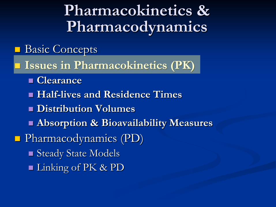
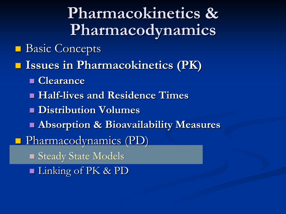
Pharmacokinetics & Pharmacodynamics
Basic Concepts Issues in Pharmacokinetics (PK)
Clearance Half-lives and Residence Times Distribution Volumes Absorption & Bioavailability Measures
Pharmacodynamics (PD) Steady State Models Linking of PK & PD
Some Resources Texts
M Rowland & RN Tozer Clinical Pharmacokinetics 4th ed., Lippincott Williams & Wilkins 2011
AJ Atkinson et al. (eds). Principles of Clinical Pharmacology, Academic Press, 3rd Edition 2012
Web sites www.cc.nih.gov/training/training/principles.html www.pharmpk.com/ (links to PK/PD resources)
Journals: Clinical Pharmacology & Therapeutics (www.ascpt.org) J. Pharmacokinetics & Pharmacodynamics
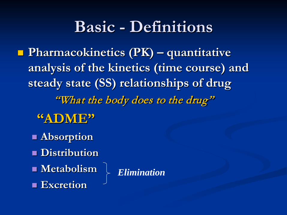
Basic - Definitions Pharmacokinetics (PK) – quantitative
analysis of the kinetics (time course) and steady state (SS) relationships of drug “What the body does to the drug”
“ADME” Absorption Distribution Metabolism Excretion
Elimination
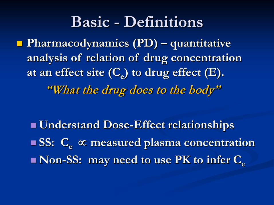
Basic - Definitions Pharmacodynamics (PD) – quantitative
analysis of relation of drug concentration at an effect site (Ce) to drug effect (E). “What the drug does to the body” Understand Dose-Effect relationships SS: Ce ∝ measured plasma concentration Non-SS: may need to use PK to infer Ce
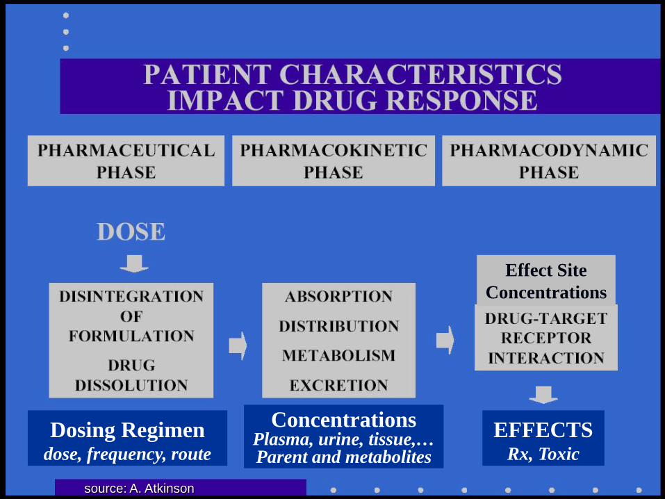
Dosing Regimen
dose, frequency, route
Concentrations
Plasma, urine, tissue,… Parent and metabolites
EFFECTS
Rx, Toxic
Effect Site Concentrations
source: A. Atkinson
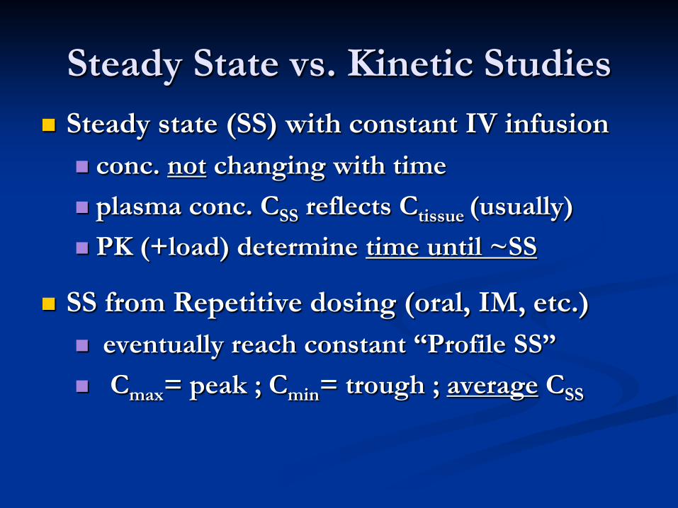
Steady State vs. Kinetic Studies Steady state (SS) with constant IV infusion conc. not changing with time plasma conc. CSS reflects Ctissue (usually)
PK (+load) determine time until ~SS
SS from Repetitive dosing (oral, IM, etc.) eventually reach constant “Profile SS” Cmax= peak ; Cmin= trough ; average CSS
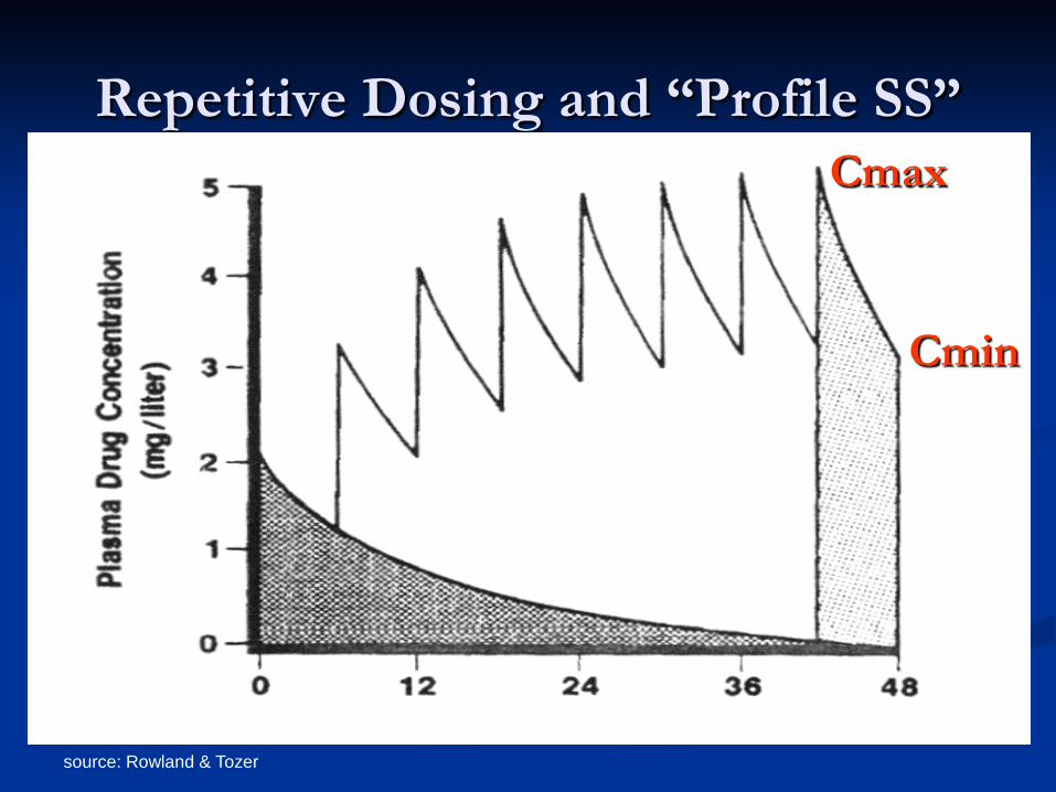
source: Rowland & Tozer
Repetitive Dosing and “Profile SS” Cmax
Cmin
Steady State vs. Kinetic Studies Many PK/PD concepts are for SS Clearance; Volume of distribution SS PD effect for given SS conc. (time to PD SS may be longer than time to plasma SS)
But some studies are kinetic e.g., single oral dose or I.V. bolus Tracer kinetic studies; PET Aim may be infer SS under rep. dosing
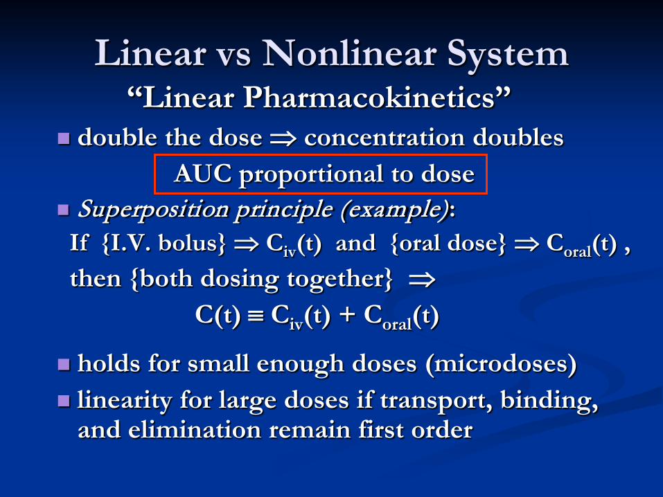
Linear vs Nonlinear System “Linear Pharmacokinetics” double the dose ⇒ concentration doubles AUC proportional to dose Superposition principle (example): If {I.V. bolus} ⇒ Civ(t) and {oral dose} ⇒ Coral(t) , then {both dosing together} ⇒ C(t) ≡ Civ(t) + Coral(t)
holds for small enough doses (microdoses) linearity for large doses if transport, binding,
and elimination remain first order
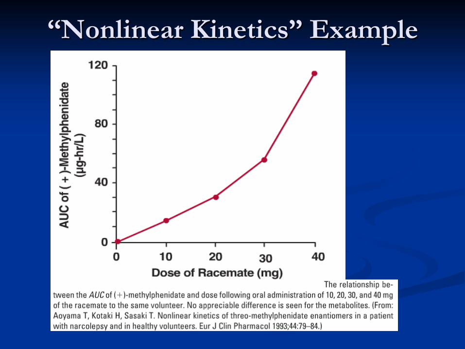
“Nonlinear Kinetics” Example
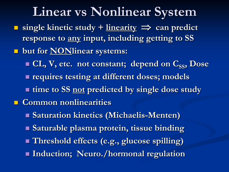
Linear vs Nonlinear System single kinetic study + linearity ⇒ can predict
response to any input, including getting to SS but for NONlinear systems:
CL, V, etc. not constant; depend on CSS, Dose requires testing at different doses; models
time to SS not predicted by single dose study Common nonlinearities
Saturation kinetics (Michaelis-Menten) Saturable plasma protein, tissue binding Threshold effects (e.g., glucose spilling) Induction; Neuro./hormonal regulation
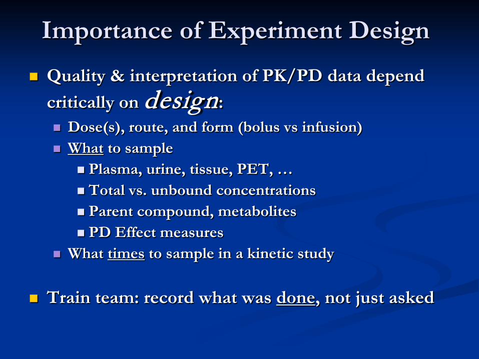
Importance of Experiment Design
Quality & interpretation of PK/PD data depend critically on design: Dose(s), route, and form (bolus vs infusion) What to sample
Plasma, urine, tissue, PET, … Total vs. unbound concentrations Parent compound, metabolites PD Effect measures
What times to sample in a kinetic study
Train team: record what was done, not just asked
Pharmacokinetics & Pharmacodynamics
Basic Concepts Issues in Pharmacokinetics (PK)
Clearance Half-lives and Residence Times Distribution Volumes Absorption & Bioavailability Measures
Pharmacodynamics (PD) Steady State Models Linking of PK & PD
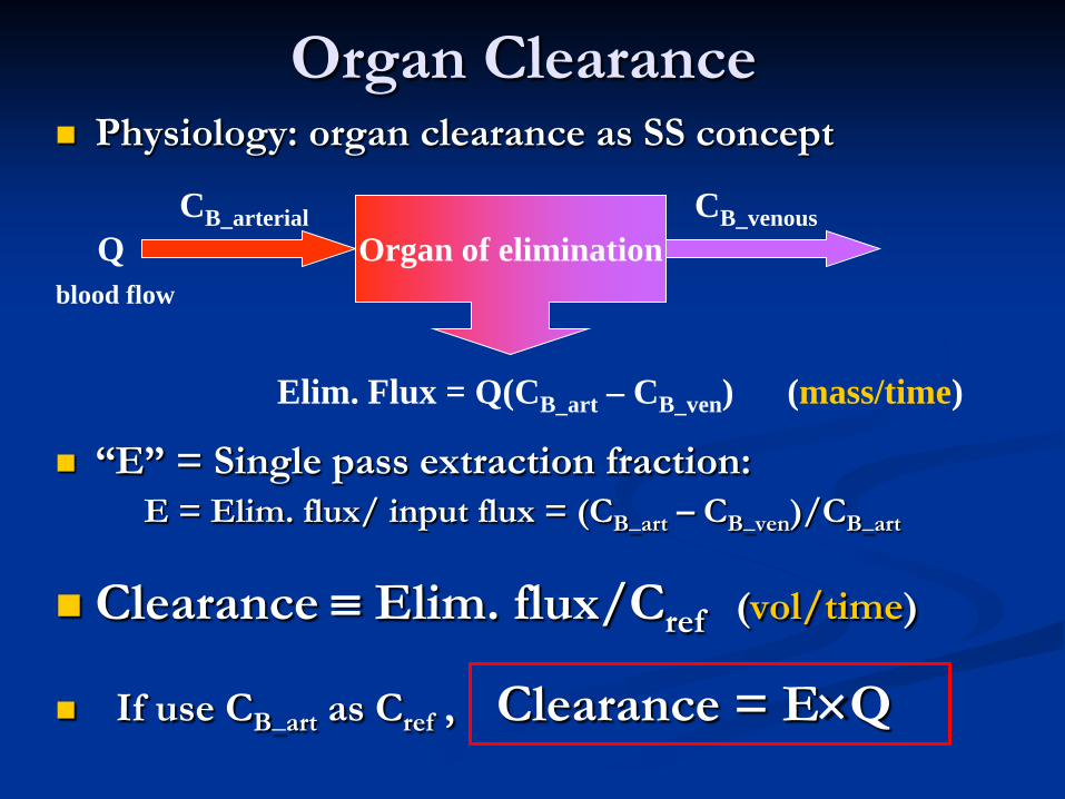
Organ Clearance Physiology: organ clearance as SS concept
“E” = Single pass extraction fraction: E = Elim. flux/ input flux = (CB_art – CB_ven)/CB_art
Clearance ≡ Elim. flux/Cref (vol/time)
If use CB_art as Cref , Clearance = E×Q
CB_arterial Organ of elimination Q
blood flow
CB_venous
Elim. Flux = Q(CB_art – CB_ven) (mass/time)
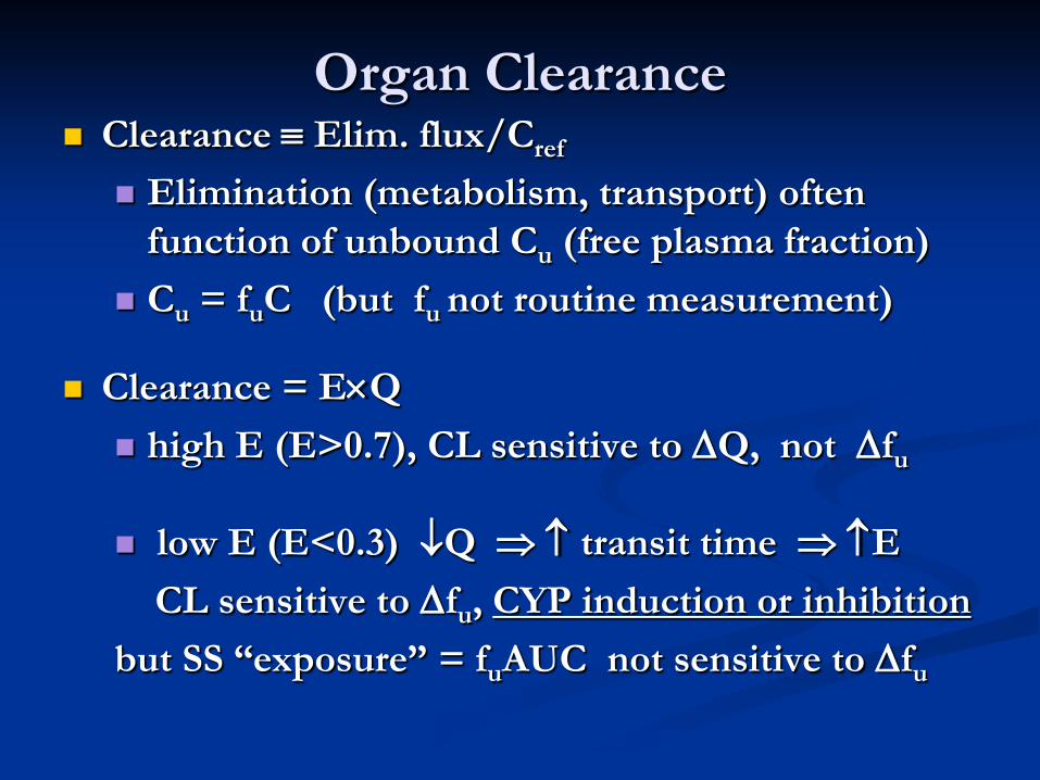
Organ Clearance Clearance ≡ Elim. flux/Cref
Elimination (metabolism, transport) often function of unbound Cu (free plasma fraction)
Cu = fuC (but fu not routine measurement)
Clearance = E×Q high E (E>0.7), CL sensitive to ∆Q, not ∆fu
low E (E<0.3) ↓Q ⇒ ↑ transit time ⇒ ↑E CL sensitive to ∆fu, CYP induction or inhibition but SS “exposure” = fuAUC not sensitive to ∆fu
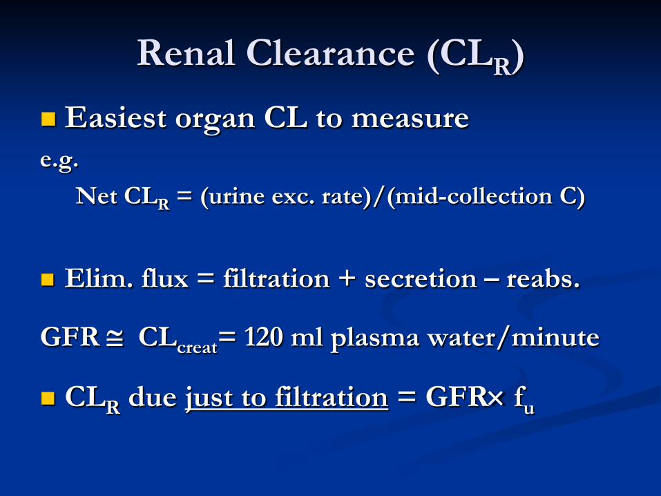
Renal Clearance (CLR) Easiest organ CL to measure e.g.
Net CLR = (urine exc. rate)/(mid-collection C)
Elim. flux = filtration + secretion – reabs.
GFR ≅ CLcreat= 120 ml plasma water/minute
CLR due just to filtration = GFR× fu
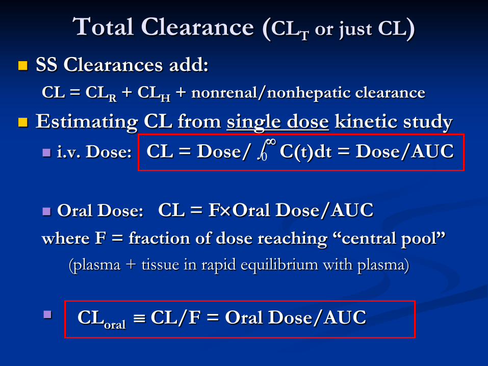
Total Clearance (CLT or just CL) SS Clearances add:
CL = CLR + CLH + nonrenal/nonhepatic clearance
Estimating CL from single dose kinetic study i.v. Dose: CL = Dose/ ∫
∞ C(t)dt = Dose/AUC Oral Dose: CL = F×Oral Dose/AUC where F = fraction of dose reaching “central pool” (plasma + tissue in rapid equilibrium with plasma)
CLoral ≡ CL/F = Oral Dose/AUC
0
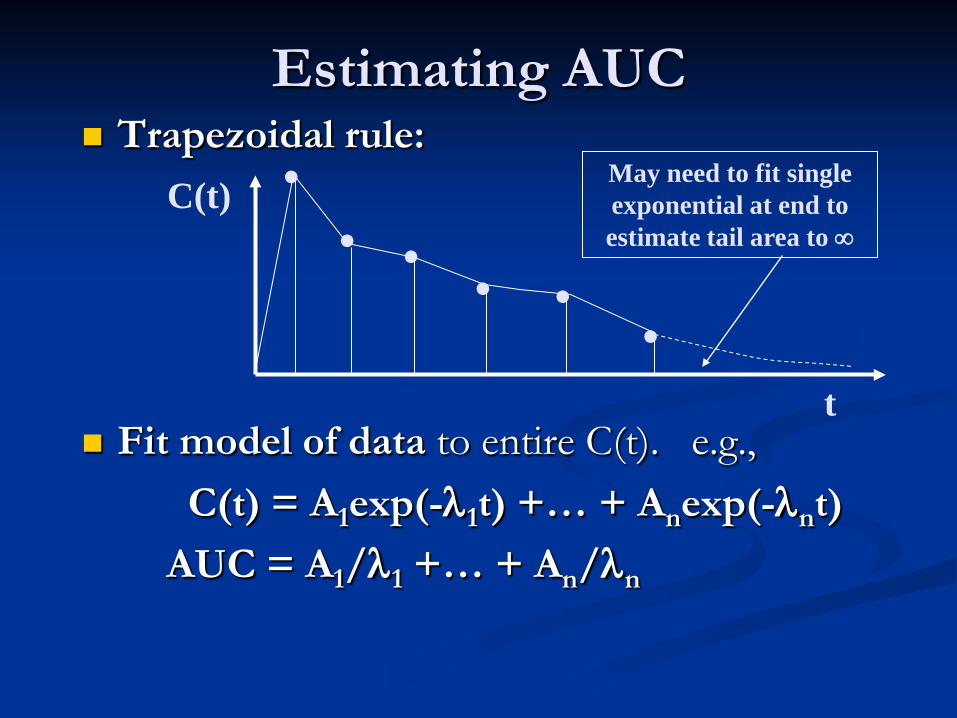
Estimating AUC Trapezoidal rule:
Fit model of data to entire C(t). e.g., C(t) = A1exp(-λ1t) +… + Anexp(-λnt) AUC = A1/λ1 +… + An/λn
. . . . . . C(t)
t
May need to fit single exponential at end to estimate tail area to ∞
source: Rowland & Tozer
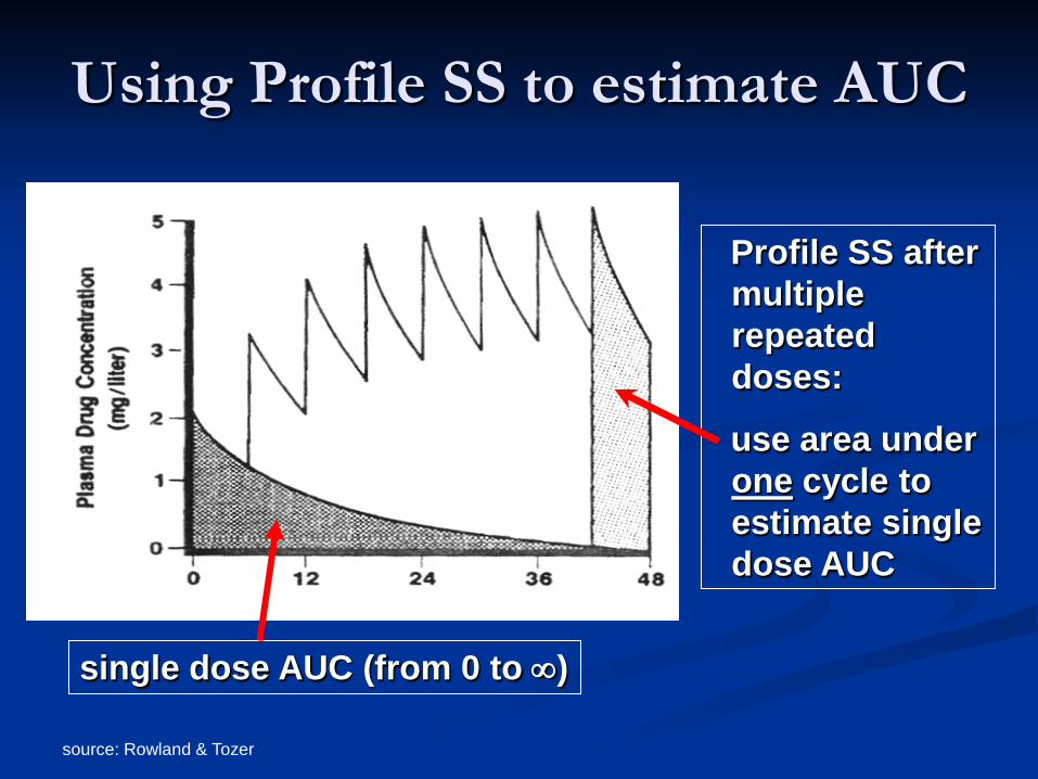
Using Profile SS to estimate AUC
single dose AUC (from 0 to ∞)
Profile SS after multiple repeated doses:
use area under one cycle to estimate single dose AUC
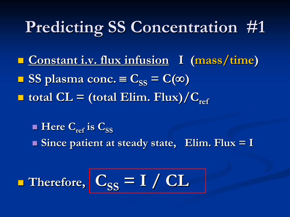
Predicting SS Concentration #1
Constant i.v. flux infusion I (mass/time) SS plasma conc. ≡ CSS = C(∞) total CL = (total Elim. Flux)/Cref
Here Cref is CSS
Since patient at steady state, Elim. Flux = I
Therefore, CSS = I / CL
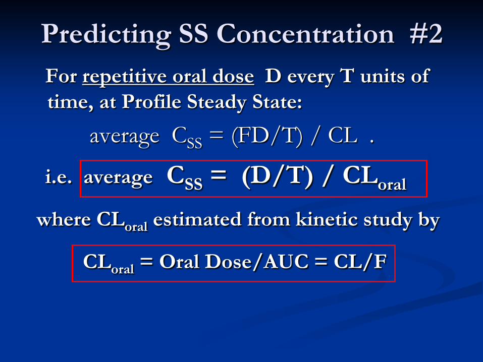
Predicting SS Concentration #2 For repetitive oral dose D every T units of
time, at Profile Steady State: average CSS = (FD/T) / CL .
i.e. average CSS = (D/T) / CLoral where CLoral estimated from kinetic study by
CLoral = Oral Dose/AUC = CL/F
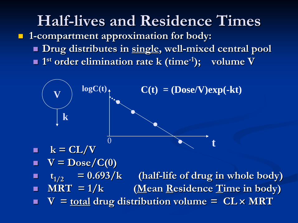
Half-lives and Residence Times 1-compartment approximation for body:
Drug distributes in single, well-mixed central pool 1st order elimination rate k (time-1); volume V
k = CL/V V = Dose/C(0) t1/2 = 0.693/k (half-life of drug in whole body) MRT = 1/k (Mean Residence Time in body) V = total drug distribution volume = CL × MRT
V C(t) = (Dose/V)exp(-kt)
t
logC(t)
k
0
. . . .
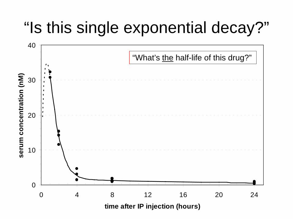
“Is this single exponential decay?”
0
10
20
30
40
0 4 8 12 16 20 24
time after IP injection (hours)
seru
m c
once
ntra
tion
(nM
)
“What’s the half-life of this drug?”
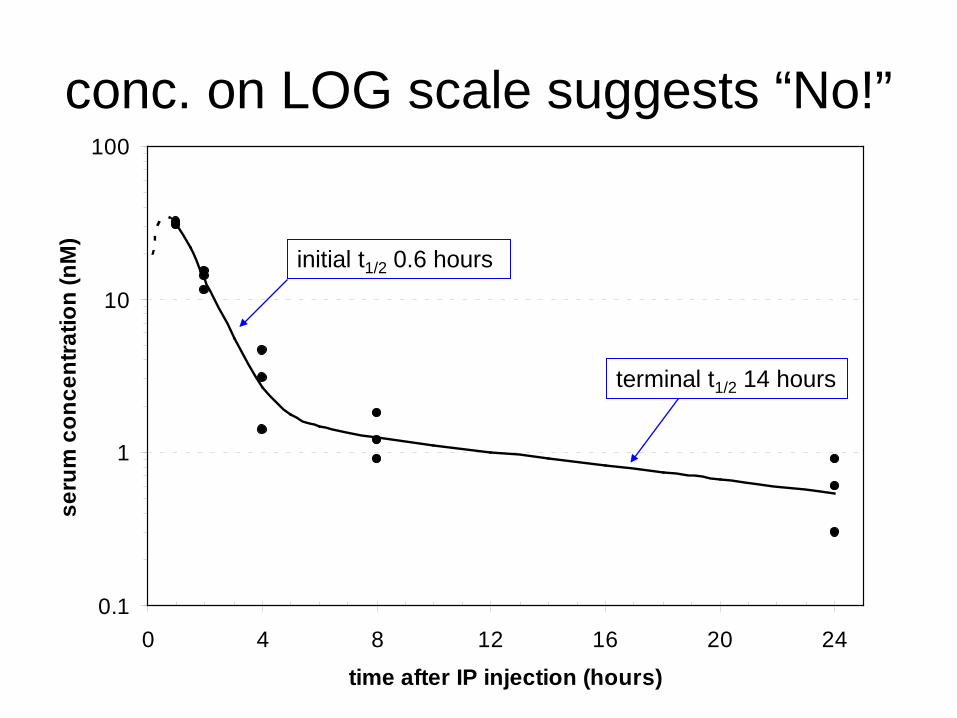
conc. on LOG scale suggests “No!”
0.1
1
10
100
0 4 8 12 16 20 24
time after IP injection (hours)
seru
m c
once
ntra
tion
(nM
)
initial t1/2 0.6 hours
terminal t1/2 14 hours
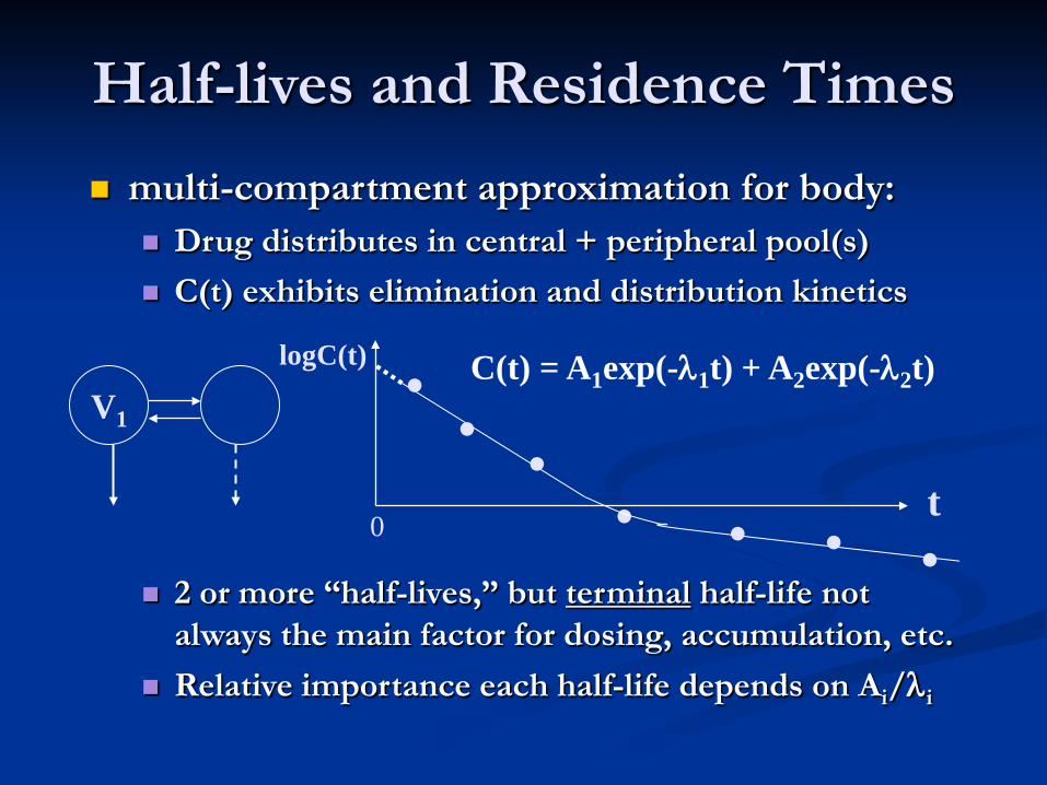
Half-lives and Residence Times multi-compartment approximation for body:
Drug distributes in central + peripheral pool(s) C(t) exhibits elimination and distribution kinetics
2 or more “half-lives,” but terminal half-life not
always the main factor for dosing, accumulation, etc. Relative importance each half-life depends on Ai/λi
V1
t
logC(t)
0
. . . . C(t) = A1exp(-λ1t) + A2exp(-λ2t)
. . .
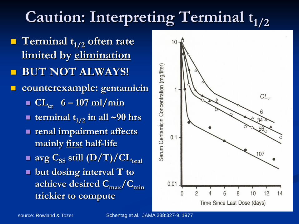
source: Rowland & Tozer Schentag et al. JAMA 238:327-9, 1977
Caution: Interpreting Terminal t1/2
Terminal t1/2 often rate limited by elimination
BUT NOT ALWAYS! counterexample: gentamicin
CLcr 6 – 107 ml/min terminal t1/2 in all ∼90 hrs renal impairment affects
mainly first half-life avg CSS still (D/T)/CLoral
but dosing interval T to achieve desired Cmax/Cmin trickier to compute
Mean Residence Time (MRT) MRT = mean time molecule of drug resides
in body before being irreversibly eliminated Assumes linear system May be useful summary measure when
there are multiple half-lives Effective (overall) half-life = 0.693×MRT
Mean Residence Time MRT estimated from a kinetic study:
Measure plasma concentration C(t) after dose:
MRT ≥ AUMC/AUC ≡ ∫ ∞tC(t)dt /AUC
MRT = AUMC/AUC requires
no “peripheral” elimination no traps linear PK
0
Mean Residence Time 1-compartment model
MRT = 1/k = V1/CL half-life = 0.693×MRT time to reach 90% SS following constant flux
infusion is 2.3 MRT’s = 3.3 half-lives
Multi-exponential model AUMC/AUC = w1(1/λ1) + … + wn(1/λn) where wi ∝ (Ai/λi ) and w1 + … + wn = 1 2.3 MRT’s (i.e., 3.3 effective half-lives) is time to
reach at least 84% SS
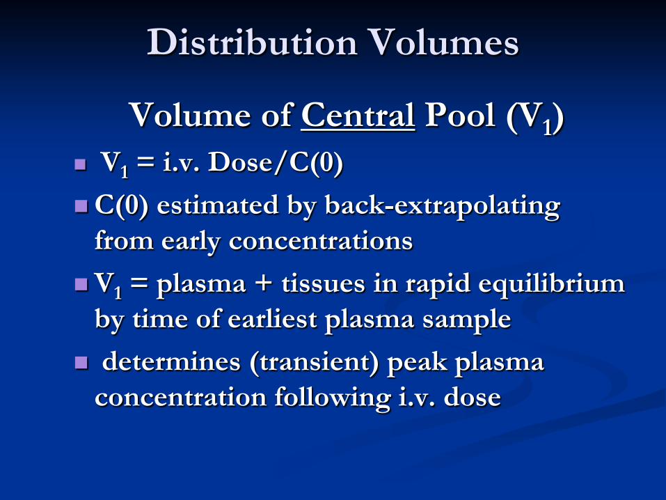
Distribution Volumes
Volume of Central Pool (V1) V1 = i.v. Dose/C(0) C(0) estimated by back-extrapolating
from early concentrations V1 = plasma + tissues in rapid equilibrium
by time of earliest plasma sample determines (transient) peak plasma
concentration following i.v. dose
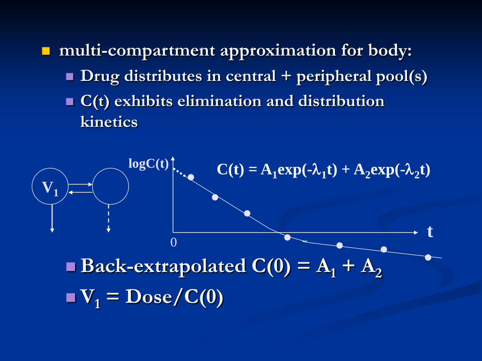
multi-compartment approximation for body: Drug distributes in central + peripheral pool(s) C(t) exhibits elimination and distribution
kinetics
Back-extrapolated C(0) = A1 + A2
V1 = Dose/C(0)
V1
t
logC(t)
0
. . . . C(t) = A1exp(-λ1t) + A2exp(-λ2t)
. . .
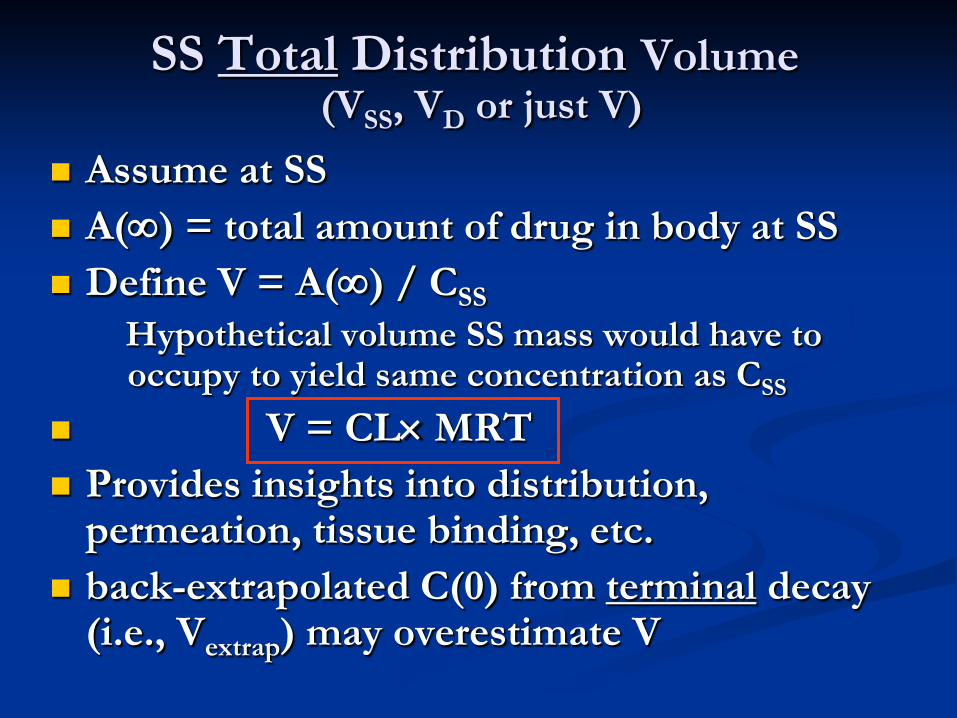
SS Total Distribution Volume (VSS, VD or just V)
Assume at SS A(∞) = total amount of drug in body at SS Define V = A(∞) / CSS
Hypothetical volume SS mass would have to occupy to yield same concentration as CSS
V = CL× MRT Provides insights into distribution,
permeation, tissue binding, etc. back-extrapolated C(0) from terminal decay
(i.e., Vextrap) may overestimate V
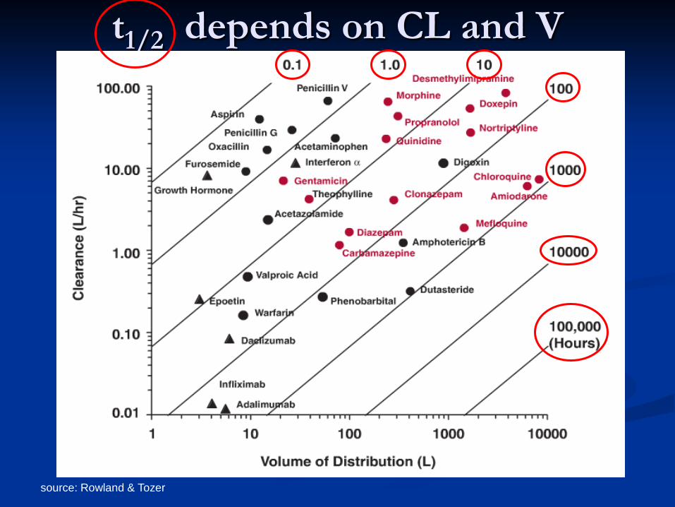
source: Rowland & Tozer
t1/2 depends on CL and V
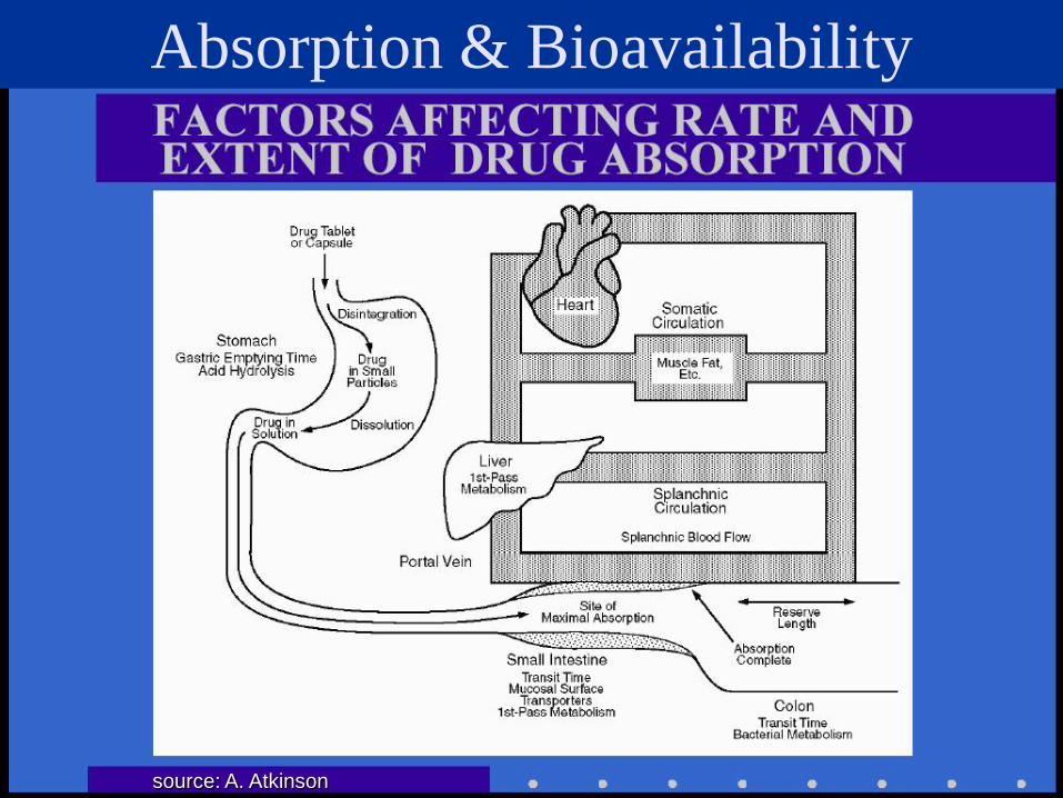
Absorption & Bioavailability
source: A. Atkinson
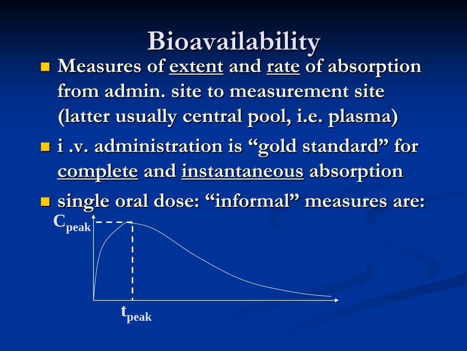
Bioavailability Measures of extent and rate of absorption
from admin. site to measurement site (latter usually central pool, i.e. plasma)
i .v. administration is “gold standard” for complete and instantaneous absorption
single oral dose: “informal” measures are:
tpeak
Cpeak
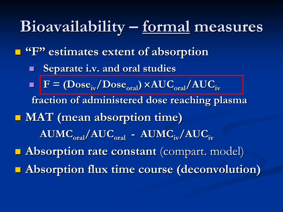
Bioavailability – formal measures “F” estimates extent of absorption
Separate i.v. and oral studies F = (Doseiv/Doseoral) ×AUCoral/AUCiv fraction of administered dose reaching plasma
MAT (mean absorption time) AUMCoral/AUCoral - AUMCiv/AUCiv
Absorption rate constant (compart. model) Absorption flux time course (deconvolution)
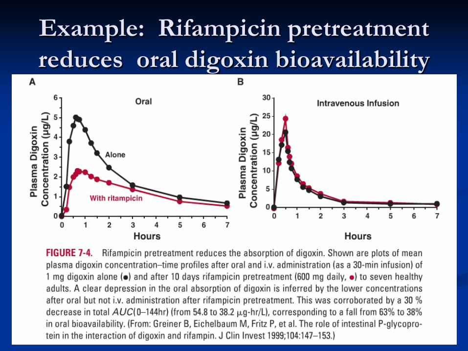
Example: Rifampicin pretreatment reduces oral digoxin bioavailability
Pharmacokinetics & Pharmacodynamics
Basic Concepts Issues in Pharmacokinetics (PK)
Clearance Half-lives and Residence Times Distribution Volumes Absorption & Bioavailability Measures
Pharmacodynamics (PD) Steady State Models Linking of PK & PD
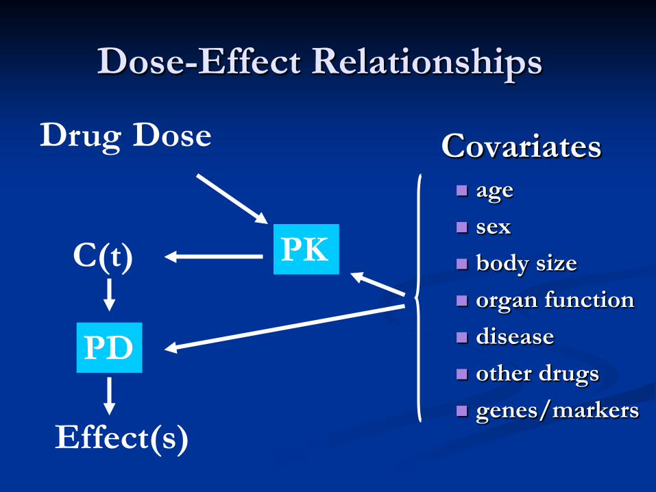
Dose-Effect Relationships
Covariates age sex body size organ function disease other drugs genes/markers
Drug Dose
Effect(s)
PK C(t)
PD
source: Frank M. Balis
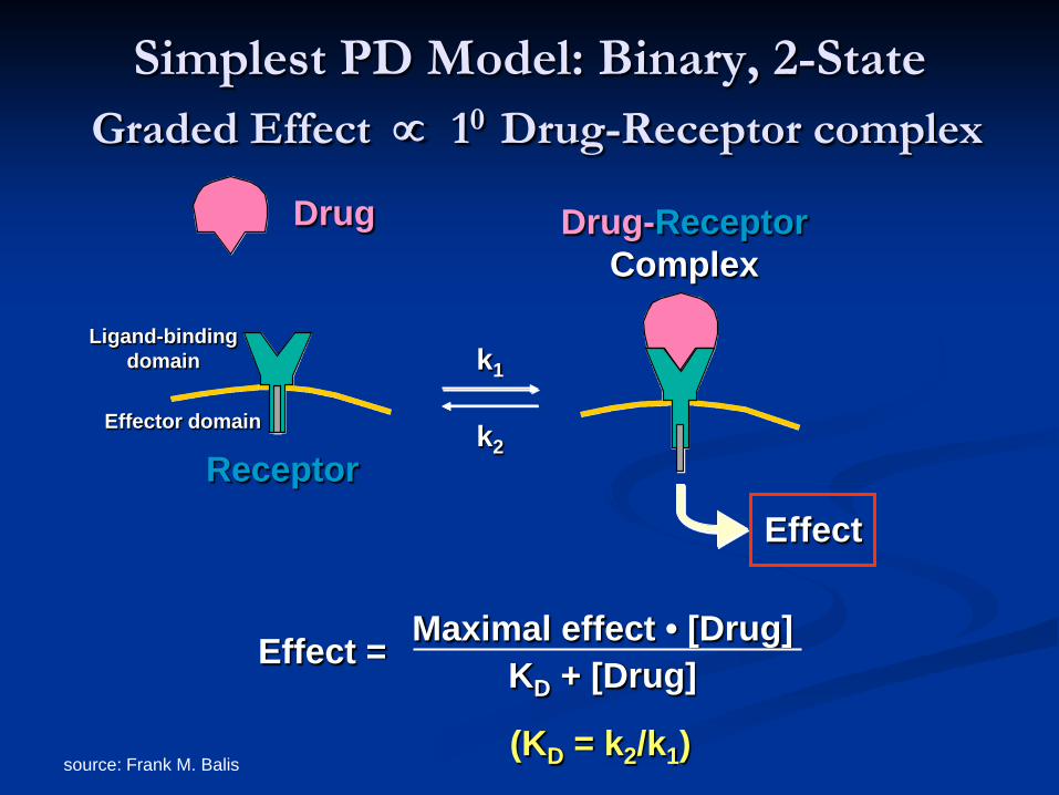
Simplest PD Model: Binary, 2-State Graded Effect ∝ 10 Drug-Receptor complex
k1
k2
Drug
Receptor Effect
Drug-Receptor Complex
Effect = Maximal effect • [Drug] KD + [Drug]
(KD = k2/k1)
Ligand-binding domain
Effector domain
source: Frank M. Balis
0
20
40
60
80
100
0 200 400 600 800
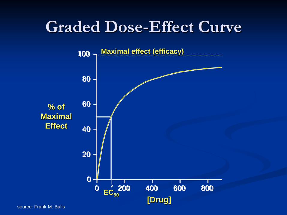
Graded Dose-Effect Curve
% of Maximal
Effect
[Drug] EC50
Maximal effect (efficacy)
source: Frank M. Balis
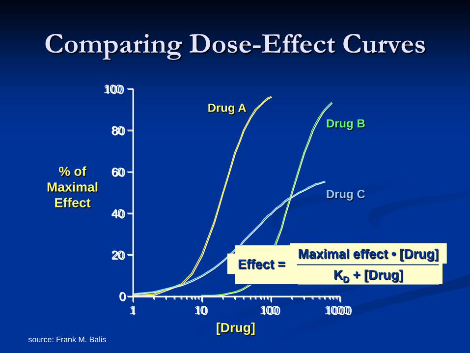
Comparing Dose-Effect Curves
0
20
40
60
80
100
1 10 100 1000
% of Maximal
Effect
[Drug]
Drug A
Drug C
Drug B
Effect = Maximal effect • [Drug]
KD + [Drug]
source: Frank M. Balis
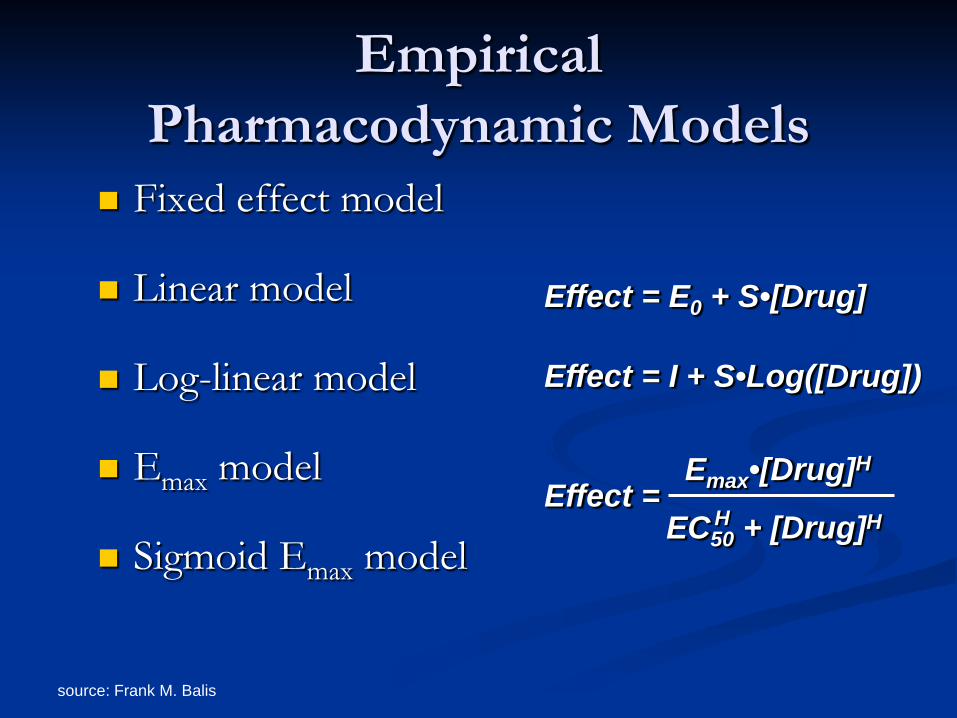
Empirical Pharmacodynamic Models
Fixed effect model
Linear model
Log-linear model
Emax model
Sigmoid Emax model
Effect = E0 + S•[Drug]
Effect = I + S•Log([Drug])
Effect = EC50 + [Drug]H
Emax•[Drug]H H
source: Frank M. Balis
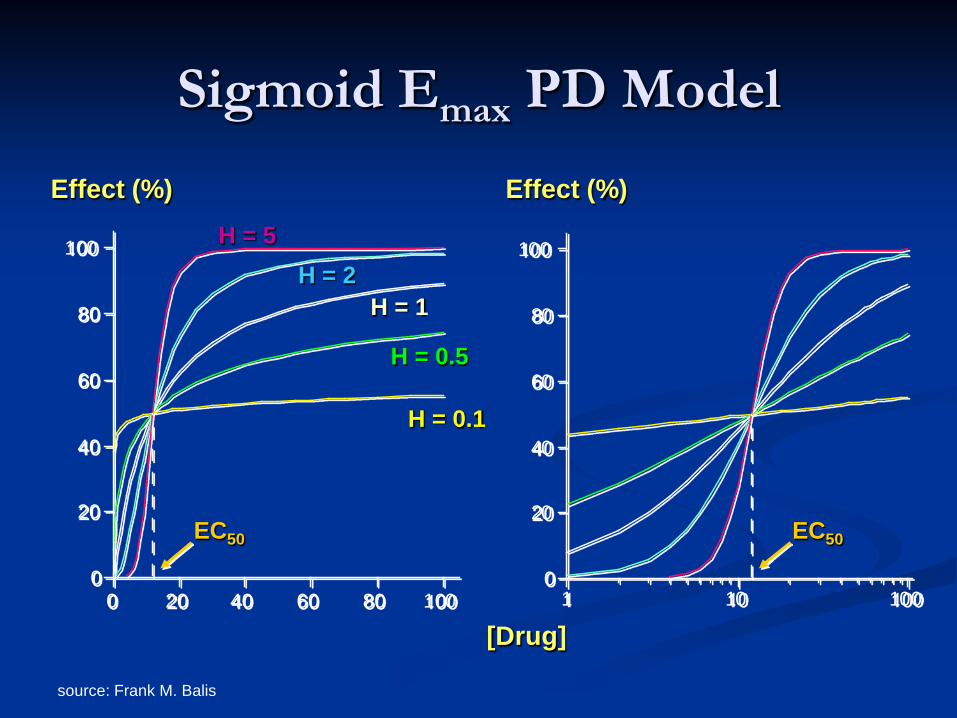
Sigmoid Emax PD Model
0
20
40
60
80
100
0 20 40 60 80 1000
20
40
60
80
100
1 10 100
[Drug]
Effect (%) Effect (%)
EC50 EC50
H = 0.1
H = 5 H = 2
H = 1
H = 0.5
source: Frank M. Balis
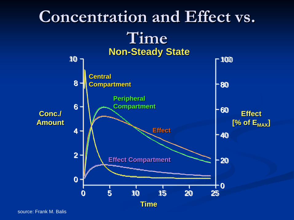
Concentration and Effect vs. Time
0
2
4
6
8
10
0
20
40
60
80
100
0 5 10 15 20 25
Conc./ Amount
Effect [% of EMAX]
Time
Central Compartment
Peripheral Compartment
Effect Compartment
Effect
Non-Steady State
source: Frank M. Balis
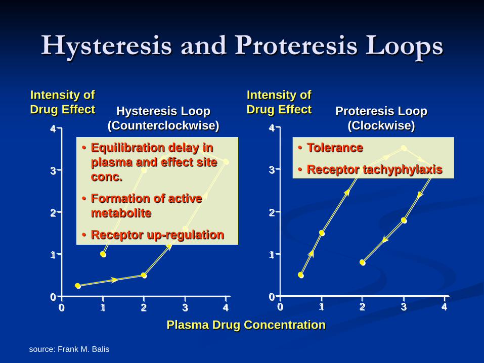
Hysteresis and Proteresis Loops
0
1
2
3
4
0 1 2 3 40
1
2
3
4
0 1 2 3 4
Plasma Drug Concentration
Intensity of Drug Effect
Intensity of Drug Effect Hysteresis Loop
(Counterclockwise) Proteresis Loop
(Clockwise)
• Equilibration delay in plasma and effect site conc.
• Formation of active metabolite
• Receptor up-regulation
• Tolerance
• Receptor tachyphylaxis
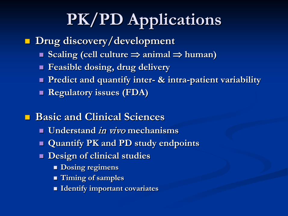
PK/PD Applications Drug discovery/development
Scaling (cell culture ⇒ animal ⇒ human) Feasible dosing, drug delivery Predict and quantify inter- & intra-patient variability Regulatory issues (FDA)
Basic and Clinical Sciences Understand in vivo mechanisms Quantify PK and PD study endpoints Design of clinical studies
Dosing regimens Timing of samples Identify important covariates
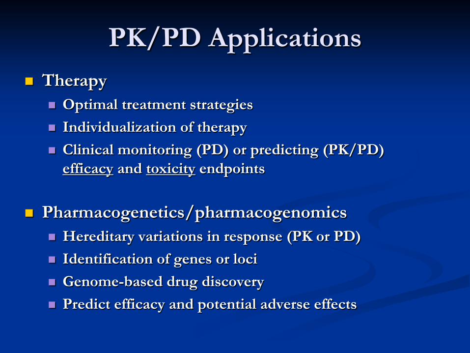
PK/PD Applications Therapy
Optimal treatment strategies Individualization of therapy Clinical monitoring (PD) or predicting (PK/PD)
efficacy and toxicity endpoints
Pharmacogenetics/pharmacogenomics Hereditary variations in response (PK or PD) Identification of genes or loci Genome-based drug discovery Predict efficacy and potential adverse effects