Embed Size (px)
Citation preview

1
Trajectories of Inertial Particles and Fluid Elements
Peter O’Malley
Physics Department
Haverford College, Haverford PA 19041
May 8th, 2008
The behavior of large or heavy particles in a fluid flow has important ramifications in nature, industry, and research, yet is not fully understood. This experiment examines the trajectories and velocities of neutrally buoyant 1 and 2 mm particles in two-dimensional fluid flows of intermediate Reynolds numbers with velocity fields varying over centimeters. The particles have Stokes numbers ranging from 2x10⁻³ to 0.6. Particle tracking is used to observe the behavior of the particles and track tracers, from which the flow velocity field is measured. Particle tracks and velocities are compared to that of ideal fluid elements and are found to be qualitatively different. Particle behavior is also unexpectedly different between the 1 and 2 mm particles: particle velocity differences from the fluid velocity vary with Stokes number for the 1 mm particles but not for the 2 mm particles.

2
Introduction
The transport of particulate matter by fluid flows occurs in a wide variety of
natural and engineering situations. For example, the formation of rain droplets by
collision in clouds is thought to depend on water particle clustering in certain regions of
the carrier air flow; the collision rate without this clustering effect is not predicted to be
high enough to explain rain formation [1]. Particle behavior in fluid flows also has
implications for industrial applications such as pollution transport [2]. Additionally,
particles are frequently used to measure fluid flows with the assumption that they follow
the flow exactly—understanding when this assumption holds is an important application
of research into particle behavior. In these and other important cases, the particles are
inertial: they have inertia relative to the flow due to their size or density and thus may
behave differently. Despite its importance, the behavior of inertial particles in fluid flows
is not fully understood.
Background
The most important parameter describing a fluid flow is the Reynolds number,
which is the ratio of inertial to viscous forces on a fluid element. It is given by
νUL=Re , (1)
where U is the mean velocity of the flow, L is the characteristic length scale of the flow,
and ν is the kinematic viscosity of the fluid. The equation governing the motion of a rigid
spherical particle in an incompressible, nonuniform fluid flow with a no-slip boundary
condition at the particle surface is given by Maxey and Riley [3] to be

3
∫
∇−−
−−
∇
+−−
∇−−−
−+=
tf
f
f
fpfp
dua
uvd
d
a
ua
uDt
D
dt
dv
ua
uva
gDt
Du
dt
dv
0
22
22
22
2
61
1
2
9
22
62
9
)(
ζζζπ
νρ
ρ
νρ
ρρρρ
, (2)
where ρp and ρf are the particle and fluid densities, respectively, v and u are the particle
and flow velocities, respectively, g is the gravitational acceleration, and a is the particle
radius. The derivative D / Dt is used to represent the time derivative following the flow,
rather than at a fixed point. The terms on the right side of the equation are, respectively,
the force of the undisturbed flow on the particle, the buoyancy force, Stokes drag, the
added mass, and the Basset-Boussinesq history force. After the equation is non-
dimensionalized, the inverse of the coefficient of the Stokes drag term is defined to be the
Stokes number, the ratio of the time it takes a particle to respond to changes in the flow to
the timescale of the flow. It is given by
Re9
22
=L
aSt
f
p
ρρ
, (3)
where L is again the length scale of the flow, and Re is the Reynolds number. The Stokes
number is thought to be the most important parameter describing the behavior of inertial
particles in a fluid flow.
Previous theoretical studies and numerical simulations have largely focused on
the phenomenon of preferential concentration, the tendency of particles to prefer certain
regions of the flow. When many particles are present in a flow, a preferential
concentration effect manifests itself as particle clustering. Balkovsky et al [4], for

4
example, predict theoretically that particle clustering should occur in turbulent flows for
heavy particles. In a numerical simulation, Bec and colleagues [5] also demonstrate
clustering by showing that inertia increases the correlation of particle positions.
Furthermore, Bec [6] also predicts, in a separate simulation, that there is a threshold
Stokes number as low as 10-4 above which particles cluster. An example of a numerical
result showing particle clustering is given in figure 1.
Furthermore, much research has been done on what flow conditions cause particle
clustering. An area of the flow can be characterized by its vorticity and strain rate. The
Okubo-Weiss parameter Q provides a numerical parameterization, defined as [7]
4/)( 22 ω−= sQ (4)
where s2, the square strain rate, is the sum of the squared normal and shear components of
the strain rate tensor and ω is the vorticity, the curl of the flow’s velocity field. Regions
of the flow with Q greater than zero are dominated by strain, while those with Q less than
zero are dominated by vorticity. Heavy particles, those whose density is greater than the
fluid, are predicted to be ejected from vortices in the flow. This effect, illustrated in
figure 2, results in the clustering of particles in regions of low vorticity and high strain
rate. A numerical simulation by Squires and Eaton [8] of heavy particles with Stokes
numbers of 0.075, 0.15 and 0.52, for example, found that particles collected in regions of
low vorticity. Eaton and Fessler’s review [9] also shows preferential concentration of
heavy particles in regions of high strain rate. Finally, Reade and Collins [10] attribute an
increase in collision rates for particles with Stokes number near unity to the increase in
particle concentration in regions of low vorticity.

5
The behavior of large particles, those with density equivalent to the fluid but large
enough to experience inertia relative to the flow, is less well understood. Babiano and
colleagues [3] show analytically that a neutrally buoyant rigid sphere of finite size will be
found preferentially in a region with a value of the Okubo-Weiss parameter specified by
its Stokes number. These preferred Okubo-Weiss values are negative; that is, particles are
predicted to avoid strain-dominated regions and settle into orbits in vorticity-dominated
regions. An example of a typical particle path is given in figure 3. Cartwright et al [11]
demonstrate that the introduction of noise forces widened the range of Stokes numbers
over which significant effects could be found. There is not universal agreement on the
behavior of large particles, however: Sapsis and Haller [12] predict theoretically that the
criterion derived by Babiano et al is an overestimate, stating instead that the criterion for
determining whether a particle follows the flow depends only on strain rate, not on
vorticity as well. In contrast to both of those predictions, Elperin et al [13] predict in
theoretical models and numerical simulations that large particles will preferentially
sample regions of high vorticity as do heavy particles. Unlike the case of heavy particles,
there is no consensus on the behavior of large particles in fluid flows.
Clustering is not the only observable property of particle behavior that varies with
particle inertia. For example, Ayyalasomayajula et al [14] show experimentally for water
droplets in wind tunnel turbulence that increasing the Stokes number decreases the
variance of the acceleration of the particles. Similarly, Qureshi et al [15] show
experimentally for large, neutrally buoyant particles in a wind tunnel flow that the
particles’ acceleration variance decreases with increasing Stokes number.

6
The behavior of inertial particles in a fluid flow is not solely determined by
effects of the flow on the particle: particle-particle interactions can have significant
effects on particle behavior as well. Many theoretical studies and numerical simulations,
however, assume low particle density and neglect any of these interactions, but because
particle clustering is often predicted, this assumption may not be valid. Bec and
colleagues [5] show that inertia can significantly enhance collision rates. The effects of
collisions can be surprising. For example, Lopez and Puglisi [16] show that collisions can
reverse the effect of inertia in some circumstances: increasing particle inertia decreases
clustering when collisions are allowed. In another numerical study [17], they predict that
these effects can also depend on the degree of elasticity (energy dissipation) of the
collisions (see figure 4).
Collisions are not the only source of particle-particle interactions: surface tension
effects can create long range attractions or repulsions between particles that are located
near interfaces. Many experimental studies, including this one, create quasi-two-
dimensional flows and have an interface as a result, so surface tension effects are a
relevant concern. Vella and Mahadevan [18] demonstrate that identical particles floating
at an interface will feel an attractive force. This attractive force will further enhance both
clustering and collision rates.
Most previous work on particle behavior has been in the turbulent regime. While
the flows in this experiment are not turbulent, previous work on large particles still
applies. In the turbulence studies, large particles have still been smaller than the smallest
scales of turbulence—that is, the velocity field is smooth on the length scale of the

7
particle. Similarly, in this experiment, the particles are significantly smaller than the scale
of the driving, and thus the velocity field is smooth on the length scale of the particle.
This experimental study examines the behavior of neutrally buoyant large
particles in two dimensional fluid flows at modest Reynolds numbers. Small tracer
particles are imaged simultaneously with large inertial particles in a two dimensional
flow and analyzed with particle tracking software. Tracer particles are assumed to behave
like ideal fluid particles and to map the flow exactly: the flow’s velocity field is derived
from their tracks. The behavior—that is, the trajectories and velocities—of the large
particles are then compared to that of the flow over a substantial range of Reynolds and
Stokes numbers. Our ability to track large numbers of tracers and particles
simultaneously makes possible statistical comparison of the dynamics of particles to the
velocity field of the flow.
Experimental Methods
We observe the behavior of particles in fluid flows with a digital camera to image
the particles and tracers to map the flow. Figure 5 gives a diagram of the experimental
setup.
The fluid consists of two layers: the top layer is 300 ml of water, while the bottom
layer is 500 ml of a salt solution of 17% potassium chloride by mass. The two layers are
created by first putting the water in troughs on either side of the cell, and then using a
syringe to inject slowly the salt solution into the bottom of the troughs, floating the water
on top of it. Once all of the salt water has been introduced in this manner, each of the

8
layers is about 4 mm deep. The two layers are miscible, which greatly reduces surface
tension, thus minimizing particle-particle interactions.
The flow is created electromagnetically: two copper electrodes placed on either
side of the cell drive a constant current through the salt solution. Directly underneath the
cell a magnet array creates a magnetic field and the Lorentz force on the ions in the fluid
creates the flow. The amount of current is varied to control the driving strength and thus
the Reynolds number. The magnet array is a square lattice of circular permanent magnets
of alternating polarization spaced 2.54 cm apart. At low Reynolds number the flow is a
steady vortex lattice, while at higher driving the flow becomes spatiotemporally chaotic
[19] (see Figure 6).
Tracers are introduced into the salt solution prior to its insertion into the cell. The
tracers are polystyrene spheres, with a radius of 80 microns. They contain a fluorescent
dye with an absorption peak of 468 nm and an emission peak of 508 nm. The large
particles are polystyrene spheres of two sizes—one set of a diameter of 2 mm and another
of 0.9 mm.
Polystyrene has a specific gravity of 1.05, while 17% KCl has a density 1.11
times that of water, so both the particles and the tracers float at the interface between the
two layers. The result is a quasi-two-dimensional flow. The particles are confined to a
single plane, and because the tracers are likewise confined to the same layer, only the
flow in that layer is observed. Furthermore, the vertical components of the flow velocity
are much smaller than the horizontal ones because the magnetic field is nearly vertical.
Thus, the buoyancy forces keeping the particles confined to a plane are greater than any
tendency of the flow to pull them away. However, the flow is not constant with depth: the

9
magnetic field increases with depth, and the top layer, being non-conducting, is not
driven, but rather dragged by the bottom layer. Additionally, as the depth increases so
does the effect of the bottom no-slip boundary of the flow. Therefore, it is important that
all the particles and tracers remain in the same plane and thus experience the same flow.
As long as the layers remain separate this is not a problem, as the particles and tracers
will always be confined to the interface. However, because the two layers are miscible,
they mix over time. As the boundary changes from a sharp interface to a smooth gradient
the particles can escape from the plane they were previously confined to and float at
different heights. The two-layer setup generally remains intact for two hours at the
strongest driving and three and a half hours at the weakest.
The observations are made with a digital camera positioned directly above the
cell. The fluid is illuminated by six blue LEDs emitting at 480 nm; a filter is placed over
the camera to eliminate the scattered blue light so the tracers are easily seen.
Diffuse white light is used to illuminate the particles. The relative intensities of these
light sources can be adjusted so that both the particles and the tracers can be seen well by
the camera. The frame rate and exposure time of the camera are controlled by an external
function generator. Higher flow speeds require a shorter exposure time to eliminate
streaking and a higher frame rate to create smoother particle tracks; however, making the
exposure time too short results in the particles and tracers being too dark to be identified.
Typical frame rates range from 10 to 25 Hz and typical exposure times are between 15
and 25 ms. The resolution of the camera is 1280 by 1024 pixels, and the viewing area is a
10 to 15 cm square. Observation runs consist of two to ten thousand frames, depending
on frame rate and the length of time the layers remain separate.

10
Data Analysis
The first step in data analysis is background subtraction. All the frames in a data
set are averaged, and the average picture is then subtracted from each individual picture.
This means that any static feature, such as a reflection, is eliminated, while the mobile
particles and tracers are unaffected. Background subtraction also helps to equalize the
brightness across the picture, as more well-lit areas are brighter on average and this is
subtracted out of all frames.
The next step after background subtraction is particle tracking. The particle
tracking algorithm was developed and implemented in the IDL language by Nicholas
Ouellette [20]. The goal of particle tracking is to determine the path each particle and
tracer takes. From this path other properties of the particle, such as its velocity, can be
determined. The particle tracking algorithm operates sequentially on each frame,
performing a series of calculations.
First, the particles and tracers must be identified. Any local maximum of intensity
greater than a threshold is considered a tracer (unless it is determined to be a big particle,
discussed below). Its x and y positions are then determined by fitting Gaussians in the x
and y directions to the intensities of the pixel and its immediate horizontal and vertical
neighbors. This gives the tracer position to a precision higher than the resolution of the
camera, about a tenth of a pixel. Contiguous groups of pixels brighter than the threshold
and larger than a minimum size are assumed to be large particles. The center of the
particle is found by a computing a weighted average of the intensities of the pixels, hence
resolving the position of the particle with a precision of about a tenth of a pixel. The

11
number of pixels required to form a particle is an adjustable parameter, which allows
tracers and large particles to be independently tracked in the same data set.
After the particles are identified the tracking algorithm must connect them to the
particles in previous frames to construct a track. For each existing track, an estimate is
made of the particle’s position in the current frame. The estimated movement of the
particle used to make this position estimate is taken to be the same as the movement of
the particle from its position two frames previously to the last frame. A circle of a given
radius is drawn around this point, and the particle closest to the center of this circle is
considered the next location in the track. If there is no particle in the circle, the track is
ended. The radius of this circle is an additional input parameter to the tracking algorithm.
If a current track does not exist two frames previously, then the track’s nearest neighbor
in the current frame is taken to be the next position. This is the case for all particles in the
second frame, for example. Finally, any particles not connected to existing tracks start
new tracks to be continued in the next frame. This is the case for all particles in the first
frame.
When all frames have been processed, the tracks are complete, and velocities for
the particles can be calculated. The x velocity at a point in a track is calculated by fitting
a parabola to the x positions of the particle from two time steps before the given point to
two after—five points in all. The y velocity is determined similarly. This method aids in
smoothing out noise in particle velocities created by uncertainties in particle positions.
The tracer tracks are then used to create a flow velocity field. First all tracer
positions and velocities are collected for a given time. These points form a velocity field
themselves: they are a set of x and y position pairs with associated x and y velocities.

12
These points are bilinearly interpolated on to a grid and smoothed with a boxcar
smoothing algorithm to provide a regular velocity field. Towards the edges of the field of
view the velocity field becomes much less accurate as there is no data outside of the
region. As a result, a border strip, typically about 50 pixels wide, is ignored in the
velocity field. The velocity of the fluid at any point can then be calculated by
interpolating from the velocity field grid. The Reynolds number of the flow can then be
determined as well: the characteristic velocity used is the RMS velocity of the flow—
calculated from the tracer data—and the length scale used is the length scale of the
driving: the magnet center spacing, 2.54 cm. After this, the Stokes number is determined
from equation (3), with the length scale again being the magnet separation.
After the construction of velocity fields the behavior of the inertial particles is
compared to fluid behavior. The most direct comparison is that of the velocity of the
large particles to the velocity of the fluid. At each particle position the flow velocity is
interpolated from the velocity field, and then the difference in speed and direction
between the particle velocity and flow velocity is calculated. Figure 7 defines the terms
used to describe these velocity differences: ∆v = |v| – |u| is the particle speed minus the
flow speed; the angular difference between the directions of the velocities is θ; and the
difference vector w = v - u is useful because its magnitude provides an unsigned measure
of speed difference, unlike ∆v, which is positive or negative depending on whether the
particle or flow is moving faster.
Another effect that can be examined is the preferential concentration of particles.
From the velocity field the strain rate and vorticity are calculated at each particle
position, and then these values are tabulated to see if the particles preferentially sample
13
certain regions of the flow. Calculating the strain rate and vorticity requires taking the
gradient of the velocity field; this is accomplished using a central difference
approximation.
Having a sequence of velocity fields for the flow over time also allows simulation
of the trajectory of an ideal fluid particle. Using Euler’s method to integrate the velocity
fields—the uncertainties in the velocity fields are large enough to make higher order
methods superfluous—the track of an ideal fluid particle can be calculated. In order to
facilitate comparison, these virtual tracks are started at instantaneous location of a
particle.
Results
The results presented here are from two data sets, one with 1 mm particles and
one with 2 mm particles. The 1 mm particle data set consists of eight runs, while the 2
mm particle data set has six runs, with each run at a different Reynolds number. Tables 1
and 2 summarize the parameters and some of the statistics of the data runs. Because the
Stokes number is linearly dependent on the Reynolds number for a given particle size,
any effects seen in a single data set could be due either to variations in the Stokes or
Reynolds number. Below, the data for each set are presented as a function of the Stokes
number, and then data sets are compared to separate these dependencies.
Figure 8 shows some sample virtual tracks together with the actual tracks from
which they were started. There are many virtual tracks for one actual track, with virtual
tracks being started one second apart along the track of the actual track. Unfortunately,
due to the amount of computation required, only a few of data runs have been analyzed in
14
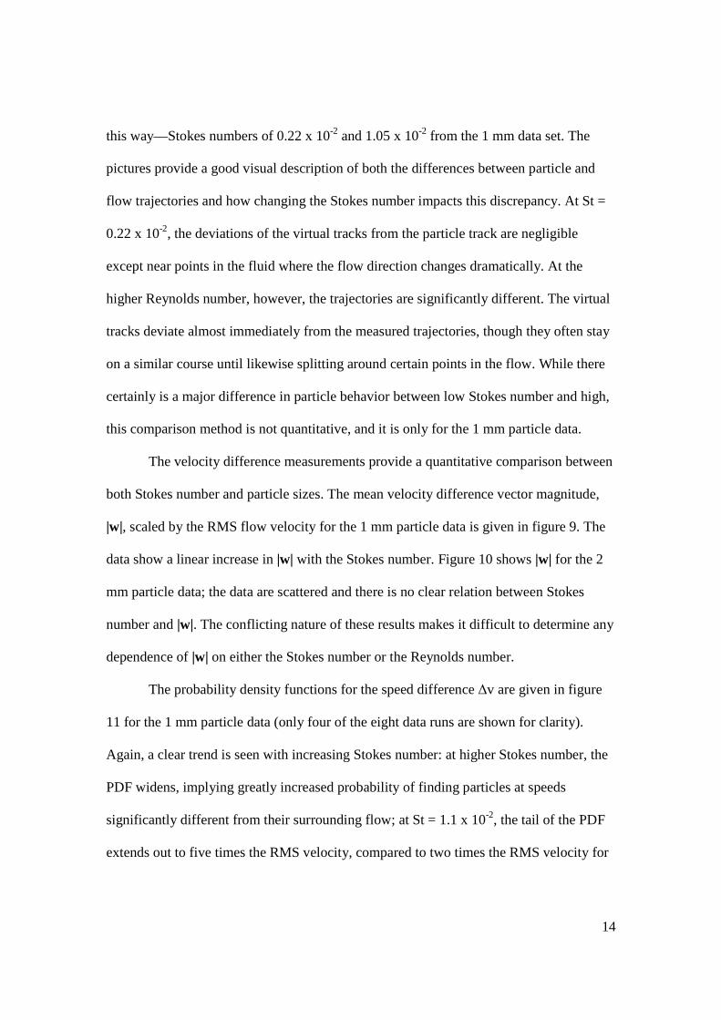
this way—Stokes numbers of 0.22 x 10⁻² and 1.05 x 10⁻² from the 1 mm data set. The
pictures provide a good visual description of both the differences between particle and
flow trajectories and how changing the Stokes number impacts this discrepancy. At St =
0.22 x 10⁻², the deviations of the virtual tracks from the particle track are negligible
except near points in the fluid where the flow direction changes dramatically. At the
higher Reynolds number, however, the trajectories are significantly different. The virtual
tracks deviate almost immediately from the measured trajectories, though they often stay
on a similar course until likewise splitting around certain points in the flow. While there
certainly is a major difference in particle behavior between low Stokes number and high,
this comparison method is not quantitative, and it is only for the 1 mm particle data.
The velocity difference measurements provide a quantitative comparison between
both Stokes number and particle sizes. The mean velocity difference vector magnitude,
|w|, scaled by the RMS flow velocity for the 1 mm particle data is given in figure 9. The
data show a linear increase in |w| with the Stokes number. Figure 10 shows |w| for the 2
mm particle data; the data are scattered and there is no clear relation between Stokes
number and |w|. The conflicting nature of these results makes it difficult to determine any
dependence of |w| on either the Stokes number or the Reynolds number.
The probability density functions for the speed difference ∆v are given in figure
11 for the 1 mm particle data (only four of the eight data runs are shown for clarity).
Again, a clear trend is seen with increasing Stokes number: at higher Stokes number, the
PDF widens, implying greatly increased probability of finding particles at speeds
significantly different from their surrounding flow; at St = 1.1 x 10⁻², the tail of the PDF
extends out to five times the RMS velocity, compared to two times the RMS velocity for

15
St = 0.2 x 10⁻². For the 2 mm particle data (figure 12), however, the PDFs are nearly
identical after being scaled by the RMS flow speed—that is, no behavior change is seen
with increasing Stokes number other than the particle velocities increasing identically
with the flow speed. Again, it is impossible to determine what effect either the Reynolds
or Stokes number has on ∆v.
The third method used for examining velocity differences is the comparison of
particle and flow direction. The probability density functions for cos(θ) are given in
figure 13 for the 1 mm particle data, again only showing four curves for clarity. There is
a clear trend: at lower Stokes number, the particle velocities are more aligned with the
flow velocity, and this alignment decreases as the Stokes number increases. Again, the 2
mm particle data (figure 14) do not display this trend, and it cannot be determined what
effect varying the Reynolds or Stokes number has on velocity alignment.
The probability density functions for sampling of the Okubo-Weiss parameter
both for 1 mm particles and tracers at the highest Stokes number are shown in figure 15.
The tracers are taken to be a representative sample of the flow, and thus by comparing the
PDFs it is possible to see if the particles preferentially sample regions dominated by
vorticity or strain. The data show a slight trend for particles to avoid regions of the
greatest vorticity and strain rate. More data are needed, however, to confirm this and
compare with the predictions of previous work.
Conclusion
The significant difference between the behavior of the particles relative to the
flow for the 1 and 2 mm cases demands that more data be taken. It is unlikely that such a
16
qualitative difference in behavior would be manifest merely due to a change in particle
size—there is an overlap both in Reynolds and Stokes numbers between the data sets, and
yet the behavior was significantly different. This difference in behavior suggests that
there may have been some experimental difference between the two data sets that has not
been accounted for. This problem can be resolved by using both sizes of particles
simultaneously—then both sizes of particles will experience the same flow in the same
conditions. However, this technique results in having fewer particles of a given size
visible at a time. This problem can be remedied, though, by taking more data—
specifically, by devoting an entire data set (the time before the two layers mix) to one
Reynolds number and now two Stokes numbers.
Despite the conflicting nature of the data analyzed so far, it is nevertheless clear
that the large particles behave significantly differently from the fluid flow. As
demonstrated by the velocity difference data, in all cases the particle velocities are
different from the flow carrying them. The characterization of these differences has
proved difficult, though, as the two different data sets disagree on whether there are
trends with changing Stokes number, and neither set shows convincing evidence of
preferential concentration.
Even after data with both particle sizes are analyzed, there is still further research
to be done. Changing the geometry of the flow—either by changing the magnet array or
by developing a new method of driving the fluid—would serve to confirm the importance
of the Stokes and Reynolds numbers by showing that the effects seen here are not unique
to this flow geometry. The flow could also be made three dimensional, through a redesign
of the experimental setup—it would require additional cameras and careful camera

17
calibration. This would require new methods of characterizing the flow, as well—though
methods for three dimensional particle tracking do exist [20]. Finally, a related case is
that of asymmetric particles, which are ubiquitous in both nature and industry. Though no
theoretical work or numerical simulations have been done on such particles, our
experimental setup could be easily extended to study them.
Acknowledgments
This experiment was conceived by Jerry Gollub and Nicholas Ouellette. I would
like to thank both of them for their constant guidance and support. The particle tracking
code was developed by Nicholas Ouellette as well, and the experimental methods and
analysis procedures were refined with the aid of Monica Kishore. Finally, I thank
Michael Jablin for many useful discussions. This work has been supported by NSF grant
DMR-0405187.

18
Figure 1: An example of fractal particle clustering in a numerical simulation by Bec [6]. This picture displays 105 particles of Stokes number 10-1.
Figure 2 (from Squires an Eaton [21]): Schematic diagram of heavy particle ejection from a region of high vorticity (bottom) into one dominated by strain (top) in a two dimensional flow. The bottom diagram shows streamlines around a vortex and the trajectory of a particle being ejected. The top diagram shows that this puts the particle into a region of high strain between vortices.

19
Figure 3: Particle track from a simulation by Babiano et al [3]; Stokes number of 0.2. The particle picks out an orbit of a fixed Q, dependent on the Stokes number of the particle.
Figure 4: Numerical simulations of Lopez and Puglisi [17]16 demonstrating particle clustering (a) in the absence of collisions and (b) under the effect of almost elastic collisions. The axes are x and y positions, and the flow is chaotically varying in space and time.

20
Figure 5: Diagram of the experimental setup, side view.
Figure 6: Sample measured velocity fields: the top is in the steady regime (Re = 30), while the bottom is chaotic (Re = 148). Blue indicates regions of vorticity, while red indicates strain.

21
Figure 7: Definition of the particle velocity, v, the flow velocity, u, and the difference w between them. The angle between v and u is denoted θ.
RMS Velocity (cm / s)
Re St (10-2)
Frames/sec (Hz)
Number of frames
0.111 30 0.22 10 2425 0.128 53 0.38 10 2466 0.174 72 0.52 10 2419 0.246 102 0.74 10 2306 0.297 123 0.90 10 2499 0.326 135 0.99 10 2531 0.345 143 1.05 10 2633 0.357 148 1.08 10 2507
Table 1: 1 mm particle data statistics.
RMS Velocity (cm / s)
Re St (10-2)
Frames/sec (Hz)
Number of frames
0.15 41 1.41 10 8000 0.23 61 2.10 10 7787 0.32 86 2.96 15 4832 0.42 112 3.86 18 5621 0.53 142 4.89 20 5621 0.64 170 5.86 25 5621
Table 2: 2mm particle data statistics.
v
u
w = v - u
θ

22
Figure 11: Virtual fluid element and actual particle trajectories for the 1 mm data set. Red solid lines are observed large particle trajectories and black dotted lines are virtual fluid
element tracks. The top two tracks are for Re = 30 and St = 0.002 x 10⁻², while the bottom three tracks have Re = 148 and St = 0.11 x 10⁻².

23
0.002 0.004 0.006 0.008 0.010 0.0120.0
0.2
0.4
0.6
0.8
1.0
Diff
eren
ce V
ecto
r M
agni
tude
/ R
MS
Vel
ocity
Stokes Number
Figure 9: Mean magnitude of the difference vector |w| vs St for 1 mm data. The particles
exhibit greater deviation from flow velocity for as the Stokes number increases.
0.01 0.02 0.03 0.04 0.05 0.060.00
0.05
0.10
0.15
0.20
0.25
0.30
0.35
0.40
0.45
0.50
0.55
0.60
Diff
eren
ce V
ecto
r M
agni
tude
/ R
MS
Vel
ocity
Stokes Number
Figure 10: Mean magnitude of the difference vector |w| vs St for 2 mm data. There is no
correlation between the Stokes number and the velocity difference.

24
-2 -1 0 1 2 3 4 51E-4
1E-3
0.01
0.1
1
10P
roba
bilit
y D
ensi
ty
Speed Difference (v-u)/(RMS Velocity)
Re St (10-2) 30 0.2 72 0.5 123 0.9 148 1.1
Figure 11: PDF of speed difference for 1 mm data for 4 runs. The deviations increase as
the Stokes number increases.
-10 -5 0 5
1E-4
1E-3
0.01
0.1
1
10
Pro
babi
lity
Den
sity
Speed Difference (v - u) / RMS Velocity
Re St (10-2) 41 1.4 86 3.0 112 3.9 170 5.9
Figure 12: PDF of speed difference for 2 mm data for 4 runs. There is minimal difference
with Stokes number.

25
0.5 0.6 0.7 0.8 0.9 1.0
1E-3
0.01
0.1
1
10
100
Re St (10-2) 30 0.2 72 0.5 123 0.9 148 1.1
Pro
babi
lity
Den
sity
Cos(theta)
Figure 13: PDF of cos(θ) for 1 mm particle data for 4 runs. There is a significant decrease
in particle and flow velocity alignment as the Stokes number increases.
0.5 0.6 0.7 0.8 0.9 1.00.01
0.1
1
10
Re St (10-2) 41 1.4 86 3.0 112 3.9 170 5.9
Pro
babi
lity
Den
sity
Cos(theta)
Figure 14: PDF of cos(θ) for 2 particle mm data for 4 runs. There is minimal change in
particle and flow velocity alignment as the Stokes number changes.

26
-0.2 0.0 0.2 0.4 0.6 0.8 1.01E-4
1E-3
0.01
0.1
1
10
100
1000P
roba
bilit
y D
ensi
ty
Q
1 mm Particles Tracers
Figure 15: PDF of Okubo-Weiss sampling for 1mm particles and tracers for Re = 148 and St = 1.08 x 10⁻². There is a slight trend for particles to prefer values of Q closer to zero.
27
References
[1]G. Falkovich, A. Fouxon and M. G. Stepanov, “Acceleration of rain initiation by could turbulence,” Nature 419, 151-154 (2002). [2] J. H. Seinfeld, Atmospheric Chemistry and Physics of Air Pollution. Wiley and Sons, New York: 1986. [3] A. Babiano, J. H. E. Cartwright, O. Piro and A. Provenzale, “Dynamics of a small neutrally buoyant sphere in a fluid and targeting in Hamiltonian systems,” Phys. Rev. Lett. 84 5764-5767 (2000). [4] E. Balkovsky, G. Falkovich and A. Fouxon, “Intermittent distribution of inertial particles in turbulent flows,” Phys. Rev. Lett. 86, 2790-2793 (2001). [5] J. Bec, A. Celani, M. Cencini and S. Musacchio, “Clustering and collision of heavy particles in random smooth flows,” Phys. Fluids 17, 073301 (2005). [6] J. Bec, “Multifractal concentrations of inertial particles in smooth random flows,” J. Fluid Mech. 528, 255-277 (2005). [7] A. Okubo, “Horizontal dispersion of floatable particles in the vicinity of velocity singularities such as convergences,” Deep-Sea Res. 17, 445 (1970). [8] K. D. Squires and J. K. Eaton, “Preferential concentration of particles by turbulence,” Phys. Fluids A 3, 1169-1178 (1991). [9] J. K. Eaton and J. R. Fessler, “Preferential concentration of particles by turbulence,” Int. J. Multiphase Flow 20, 169-209 (1994). [10] W. C. Reade and L. R. Collins, “Effect of preferential concentration on turbulent collision rates,” Phys. Fluids 12, 2530-2540 (2000). [11] J. H. E. Cartwright, M. O. Magnasco and O. Piro, “Noise- and inertia-induced inhomogeneity in the distribution of small particles in fluid flows,” Chaos 12, 489-495 (2002). [12] T. Sapsis and G. Haller, “Instabilities in the dynamics of neutrally buoyant particles,” Phys. Fluids 20, 017102 (2008). [13] T. Elperin, N. Kleeorin, V. S. L’vov, I. Rogachevskii and D. Sokoloff, “Clustering instability of the spatial distribution of inertial particles in turbulent flows,” Phys. Rev. E 66, 036302 (2002). [14] S. Ayyalasomayajula, A. Gylfason, L. R. Collins, E. Bodenschatz and Z. Warhaft, “Lagrangian measurements of inertial particle accelerations in grid generated wind tunnel turbulence,” Phys. Rev. Lett. 97, 114507 (2006).

28
[15] N. Qureshi, M. Bourgoin, C. Baudet, A. Cartellier and Y. Gagne, “Turbulent transport of material particles: An experimental study in finite size effects,” Phys. Rev. Lett. 99, 184502 (2007). [16] C. Lopez and A. Puglisi, “Continuum description of finite-size particles advected by external flows: The effect of collisions,” Phys. Rev. E 69, 046306 (2004). [17] C. Lopez and A. Puglisi, “Sand stirred by chaotic advection,” Phys. Rev. E. 67, 041302 (2003). [18] D. Vella and L. Mahadevan, “The ‘Cheerios effect,’” Am. J. Phys. 73, 817-825 (2005). [19] N. T. Ouellette and J. P. Gollub, “Curvature fields, topology, and the dynamics of spatiotemporal chaos,” Phys. Rev. Lett. 99, 194502 (2007). [20] N. T. Ouellette, H. Xu, E. Bodenshatz, “A quantitative study of three-dimensional Lagrangian particle tracking algorithms,” Experiments in Fluids 40, 301-313 (2006). [21] K. D. Squires and J. K. Eaton, “Particle response and turbulence modification in isotropic turbulence,” Phys. Fluids A 2, 1191-1203 (1990).