TRANSACTIONS ON VISUALIZATION AND …sandre17/blendedFORKS/blended... · 2015-06-21 · We call the resulting model a ﬁrst order reduced compliant ... alternative elastic simulation

TRANSACTIONS ON VISUALIZATION AND COMPUTER GRAPHICS, VOL. ?, NO. ?, R? 201? 1

Blended linear models forreduced compliant mechanical systems

Sheldon Andrews, Member, IEEE, Marek Teichmann, Paul G. Kry

Abstract—We present a method for the simulation of compliant, articulated structures using a plausible approximate model thatfocuses on modeling endpoint interaction. We approximate the structure’s behavior about a reference configuration, resulting in a firstorder reduced compliant system, or FORK-1S. Several levels of approximation are available depending on which parts and surfaces wewould like to have interactive contact forces, allowing various levels of detail to be selected. Our approach is fast and computation ofthe full structure’s state may be parallelized. Furthermore, we present a method for reducing error by combining multiple FORK-1Smodels at different linearization points, through twist blending and matrix interpolation. Our approach is suitable for stiff, articulategrippers, such as those used in robotic simulation, or physics-based characters under static proportional derivative control. Wedemonstrate that simulations with our method can deal with kinematic chains and loops with non-uniform stiffness across joints, andthat it produces plausible effects due to stiffness, damping, and inertia.

Index Terms—character animation, physics simulation, constraints

F

1 INTRODUCTION

R EAL-TIME physics simulation has emerged as a fun-damental component of interactive immersive virtual

environments. There are important applications in operatortraining for robots and heavy equipment, robotic design,and simulation of virtual humans in video games.

In this paper, we describe a technique that improves in-teractive simulations involving complex multi-body mecha-nisms with contact. For instance, the simulation of human orrobotic hands during grasping involves complicated chainsof compliant joints and distributed contacts. Collaborativegrasping and manipulation with multiple people, multi-legged robots, and vehicle suspension systems can producesimilarly difficult computational scenarios. Simulating thesekinds of systems is tricky because they result in large over-constrained systems of equations that may require consid-erable computational effort to solve. Furthermore, specialattention must be paid to the parameters of both the systemand simulation to ensure stability. Our technique simplifiesthese kinds of systems, allowing for complex mechanismsto be simulated while meeting real-time requirements.

Our approach is based on two main assumptions. Thefirst assumption is that there are a limited number ofsurfaces at which articulated systems experience contact.Thus, we focus on the effective mechanical properties of asmall collection of bodies in the system. This is a reasonableassumption for many scenarios, such as the wheel groundcontact for a vehicle, the fingertips of a hand during grasp-ing, or simulated tool-use by virtual humans and robots.The second assumption is that the multi-body system hasa reference pose, which is held due to linear springs at thejoints. This is certainly true for systems that have passivelinear elastic joints, but also reasonable for virtual humans

• Sheldon Andrews and Paul G. Kry are with the School of ComputerScience, McGill University, Montreal, QC, Canada. Marek Teichmannis with CMLabs, Montreal, QC, Canada.

Manuscript received March, 2015.

following the equilibrium point hypothesis of motor control,and in simulated robots using proportional derivative (PD)control.

In the case of a single interaction surface, our approachsimplifies an entire system to a single 6D mass-springsystem. When there are multiple bodies with surfaces ex-periencing contact, we use a collection of compliantly cou-pled 6D bodies. We present an incremental algorithm thatwalks the body connectivity graph to compute the dynamicsmodel. The result is a system that is much simpler than theoriginal, and is also stable and fast to compute. Note thatwe do not assume that the structure has the topologicalstructure of a tree, as is necessary for fast computation inmany alternative multi-body algorithms.

We call the resulting model a first order reduced compliantsystem, abbreviated as FORK-1S. The method descriptionand model construction originally described by Andrews etal. [1] are presented in this article with additional numericaldetails and with numerous edits focused on improving clar-ity (for example, the use of compliance matrices instead ofinverse stiffness). In this article we also present an importantextension to the original FORKS model. We show how tocombine multiple FORK-1S models at different linearizationpoints to reduce simulation errors over a wider range of thestate space.

For a single FORK-1S model at simulation time, externalforces produce a dynamic transient behavior for the bodiesthat we include in the model. The positions of all the remain-ing bodies are visualized by computing a compatible state.Rather than using inverse kinematics, we compute linearmaps that provide twists for each body as a function ofthe reduced system state. With these maps, we then use theexponential map to compute the body positions. Thus, non-interacting body positions can be computed independentlyand in a parallel fashion. Although the twists only modelthe linear response, we observe that the exponential mapgives good behavior with little separation at joints for an


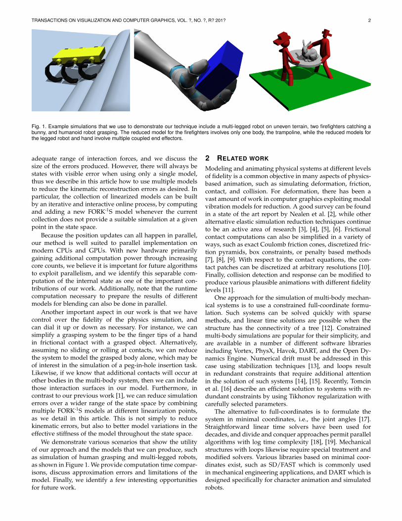
Fig. 1. Example simulations that we use to demonstrate our technique include a multi-legged robot on uneven terrain, two firefighters catching abunny, and humanoid robot grasping. The reduced model for the firefighters involves only one body, the trampoline, while the reduced models forthe legged robot and hand involve multiple coupled end effectors.

adequate range of interaction forces, and we discuss thesize of the errors produced. However, there will always bestates with visible error when using only a single model,thus we describe in this article how to use multiple modelsto reduce the kinematic reconstruction errors as desired. Inparticular, the collection of linearized models can be builtby an iterative and interactive online process, by computingand adding a new FORK-1S model whenever the currentcollection does not provide a suitable simulation at a givenpoint in the state space.

Because the position updates can all happen in parallel,our method is well suited to parallel implementation onmodern CPUs and GPUs. With new hardware primarilygaining additional computation power through increasingcore counts, we believe it is important for future algorithmsto exploit parallelism, and we identify this separable com-putation of the internal state as one of the important con-tributions of our work. Additionally, note that the runtimecomputation necessary to prepare the results of differentmodels for blending can also be done in parallel.

Another important aspect in our work is that we havecontrol over the fidelity of the physics simulation, andcan dial it up or down as necessary. For instance, we cansimplify a grasping system to be the finger tips of a handin frictional contact with a grasped object. Alternatively,assuming no sliding or rolling at contacts, we can reducethe system to model the grasped body alone, which may beof interest in the simulation of a peg-in-hole insertion task.Likewise, if we know that additional contacts will occur atother bodies in the multi-body system, then we can includethose interaction surfaces in our model. Furthermore, incontrast to our previous work [1], we can reduce simulationerrors over a wider range of the state space by combiningmultiple FORK-1S models at different linearization points,as we detail in this article. This is not simply to reducekinematic errors, but also to better model variations in theeffective stiffness of the model throughout the state space.

We demonstrate various scenarios that show the utilityof our approach and the models that we can produce, suchas simulation of human grasping and multi-legged robots,as shown in Figure 1. We provide computation time compar-isons, discuss approximation errors and limitations of themodel. Finally, we identify a few interesting opportunitiesfor future work.

2 RELATED WORK

Modeling and animating physical systems at different levelsof fidelity is a common objective in many aspects of physics-based animation, such as simulating deformation, friction,contact, and collision. For deformation, there has been avast amount of work in computer graphics exploiting modalvibration models for reduction. A good survey can be foundin a state of the art report by Nealen et al. [2], while otheralternative elastic simulation reduction techniques continueto be an active area of research [3], [4], [5], [6]. Frictionalcontact computations can also be simplified in a variety ofways, such as exact Coulomb friction cones, discretized fric-tion pyramids, box constraints, or penalty based methods[7], [8], [9]. With respect to the contact equations, the con-tact patches can be discretized at arbitrary resolutions [10].Finally, collision detection and response can be modified toproduce various plausible animations with different fidelitylevels [11].

One approach for the simulation of multi-body mechan-ical systems is to use a constrained full-coordinate formu-lation. Such systems can be solved quickly with sparsemethods, and linear time solutions are possible when thestructure has the connectivity of a tree [12]. Constrainedmulti-body simulations are popular for their simplicity, andare available in a number of different software librariesincluding Vortex, PhysX, Havok, DART, and the Open Dy-namics Engine. Numerical drift must be addressed in thiscase using stabilization techniques [13], and loops resultin redundant constraints that require additional attentionin the solution of such systems [14], [15]. Recently, Tomcinet al. [16] describe an efficient solution to systems with re-dundant constraints by using Tikhonov regularization withcarefully selected parameters.

The alternative to full-coordinates is to formulate thesystem in minimal coordinates, i.e., the joint angles [17].Straightforward linear time solvers have been used fordecades, and divide and conquer approaches permit parallelalgorithms with log time complexity [18], [19]. Mechanicalstructures with loops likewise require special treatment andmodified solvers. Various libraries based on minimal coor-dinates exist, such as SD/FAST which is commonly usedin mechanical engineering applications, and DART which isdesigned specifically for character animation and simulatedrobots.


Our approach resembles neither a minimal coordinateor redundant coordinate constrained multi-body system.Instead, our first order reduced compliant systems moreclosely resemble coupled elastic mass-spring systems. Wenote that other approaches have been proposed for reducingmulti-body dynamics. For example, adaptive dynamics ispossible in reduced coordinates through rigidification of se-lected joints [20]. In contrast, with a constrained redundantcoordinate formulation, modal reduction of rigid articulatedstructures is possible and has been used to animate characterlocomotion [21], [22].

We observe that inverse kinematics techniques wouldalso be a solution for determining the positions of internalparts of the mechanism. There are a variety of fast meth-ods for solving over-constrained inverse kinematics prob-lems using singularity-robust inverse computations [23] ordamped least squares [24]. Instead, we opt for the computa-tion of each body individually with a twist because each canbe updated in parallel, providing a constant time solution.While typically unnoticeable for small motions, we evaluatehow joint constraint violations grow and discuss options tominimize or avoid visible errors during larger interactionforces by interpolating multiple linear models.

End effector equations of motion are important in robotcontrol and analysis, and projections of system dynamics area central part of the operational space formulation of Khatib[25]. Our incremental projection of the dynamics producesa similar model. In contrast, effective end-point dynamicscan also be estimated from data. For instance, model fit-ting has been applied to human fingertips and hands [26],[27]. In our case, a dynamics projection approach is prefer-able because the fitting process can become difficult whendata is complex. Fitting a simple 6D linear mass-spring isundesirable when the force to displacement relationshipin the full model exhibits non-linearities and bifurcationbehavior. Furthermore, sampling the system behavior canbe expensive and does not fit the desired work flow ofinteractive simulators. However, it is not unreasonable toimpose such a simple model, and to identify its behaviorbased on a projection of linear compliant or PD controlledbehavior of joints. Ultimately, our simplification producesan inexpensive first order model with a plausible responsecorresponding to a slightly modified set of non-linear jointcontrollers.

We use concepts of 6D rigid motion in this paper. Thebook by Murray et al. [28] includes a good overview of themathematics of rigid motion, twists, wrenches, and adjointtransformations between different coordinate systems. Wealso provide a brief introduction to rigid body kinematicsand related definitions in the Appendix.

Finally, note that this work extends that of Andrewset al. [1]. We include in this article the formulation of theFORK-1S model, but we make a number of improvementsfor clarity. For instance, compliance matrices are not denotedas an inverse of a stiffness in this article so as to avoid theconfusion when the stiffness is not invertible. We add someadditional explanations and adjust notation in Sections 3,4, and 5. Our extensions to multiple linearized models aredescribed in Section 7, and the improvements that thisbrings are evaluated and discussed in Section 8.

3 DYNAMICS PROJECTION AND NOTATION

Our method targets mechanisms made up of articulatedchains of compliant joints where external interaction occursonly with a small collection of bodies at the interface. Wecall these bodies the end effectors, following the terminol-ogy used in robotics literature. For simplicity, we initiallypresent our approach for the case where the base, or root,of the mechanical system is fixed in the world (the caseof a free-body base link is discussed in Section 6). Thereare numerous simulation and animation applications wherethis type of configuration occurs, such as the grasping andmanipulation examples described in Section 1.

In this section, we first explore the simple case of dy-namics projection for a single body with one rotationaljoint, and provide a preliminary discussion of how we canincrementally build a projection for a complex mechanicalsystem.

3.1 Projection for a single link

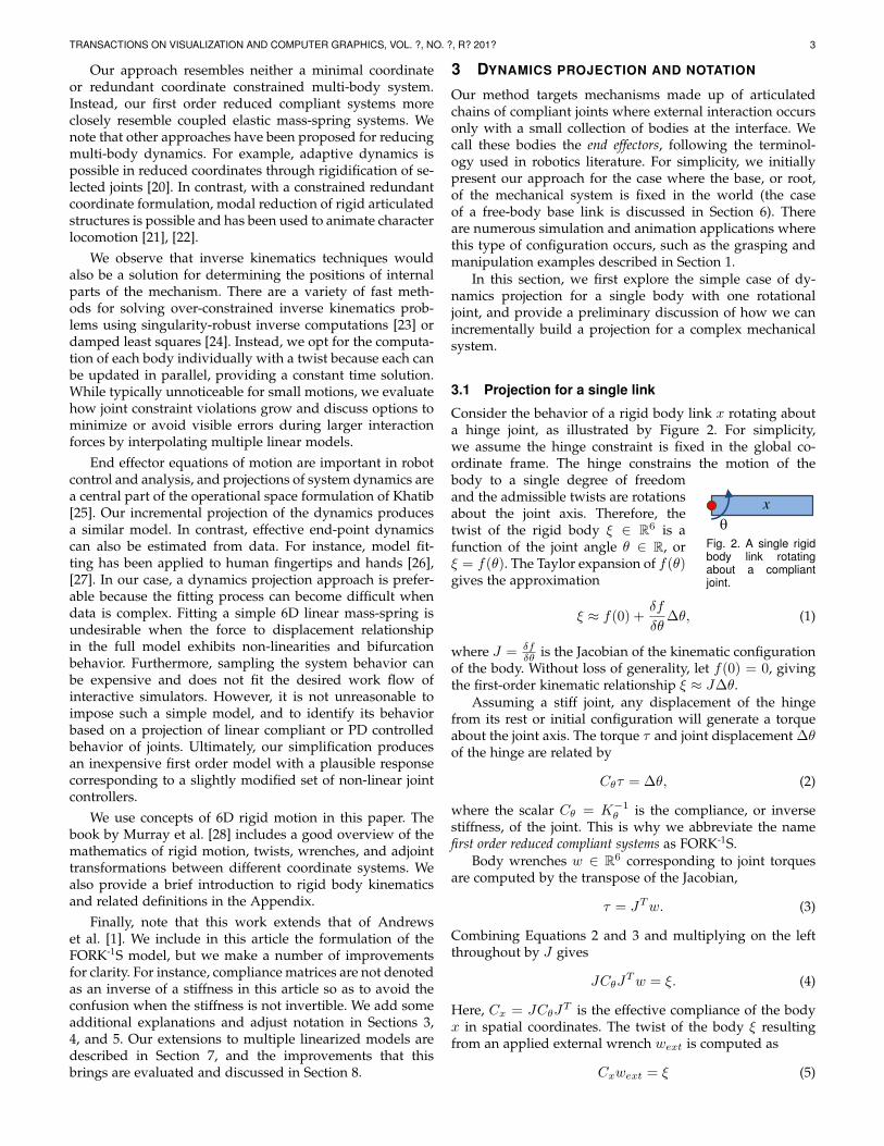
Consider the behavior of a rigid body link x rotating abouta hinge joint, as illustrated by Figure 2. For simplicity,we assume the hinge constraint is fixed in the global co-ordinate frame. The hinge constrains the motion of the

qx

Fig. 2. A single rigidbody link rotatingabout a compliantjoint.

body to a single degree of freedomand the admissible twists are rotationsabout the joint axis. Therefore, thetwist of the rigid body ξ ∈ R6 is afunction of the joint angle θ ∈ R, orξ = f(θ). The Taylor expansion of f(θ)gives the approximation

ξ ≈ f(0) +δf

δθ∆θ, (1)

where J = δfδθ is the Jacobian of the kinematic configuration

of the body. Without loss of generality, let f(0) = 0, givingthe first-order kinematic relationship ξ ≈ J∆θ.

Assuming a stiff joint, any displacement of the hingefrom its rest or initial configuration will generate a torqueabout the joint axis. The torque τ and joint displacement ∆θof the hinge are related by

Cθτ = ∆θ, (2)

where the scalar Cθ = K−1θ is the compliance, or inversestiffness, of the joint. This is why we abbreviate the namefirst order reduced compliant systems as FORK-1S.

Body wrenches w ∈ R6 corresponding to joint torquesare computed by the transpose of the Jacobian,

τ = JTw. (3)

Combining Equations 2 and 3 and multiplying on the leftthroughout by J gives

JCθJTw = ξ. (4)

Here, Cx = JCθJT is the effective compliance of the body

x in spatial coordinates. The twist of the body ξ resultingfrom an applied external wrench wext is computed as

Cxwext = ξ (5)


and the homogeneous transformation of the body’s dis-placement is computed by the exponential map. Specifi-cally, we denote Hξ as the 4-by-4 homogeneous transfor-mation matrix of a body displaced by twist ξ from the restconfiguration and compute it as

Hξ = H exp(ξ), (6)

where H is the transformation matrix of the body in the therest configuration (additional comments with respect to thismatrix exponential appear in the appendix).

It is convenient to use compliance to model the behaviorof the body in full coordinates because this compliance willbe zero for motions not permitted by the joint. As such, Cxcan be rank deficient, and a robust method for computingthe matrix inverse is necessary to compute the stiffness Kx.Our work uses a truncated singular value decomposition(SVD) [29] to compute the inverse when needed.

We can perform a very similar projection of the rotationalmass matrix Mθ by working with the inverse mass A =M−1, which we define as accelerability. From the equationof motion Aθτ = θ, and assuming the body accelerationφ ∈ R6 is approximately Jθ, we find JAθJTw = φ, thus,

Ax = JAθJT . (7)

We follow the same projection for the damping matrix toproduce the second order system

Mxφ+Dxφ+Kxξ = w. (8)

Note that the static solution of this system exactly matchesthat of the original. Also notice that this example is moreinstructional than useful given that Equation 8 has sixdimensions while it was constructed from a 1D joint. Thatis, Equation 8 is rank one in this case and requires that weproduce a solution within the space of admissible motions.In contrast, many of the larger more complex examples weshow in this paper result in full rank systems.

Despite the simplicity of this example, these projectionsare useful and a central part of the approach we describein Section 4. Specifically, the end effector will be part ofa complex system of joints and rigid bodies. The effectivecompliance at the end effector x is due not only to thecompliant behavior of the directly attached joint, but alsodepends on the compliance of its parent (and the rest of thesystem). As such, we will describe an incremental approachfor computing the effective stiffness, damping, and mass, ateach link in an articulated system.

3.2 Truncated SVD toleranceMatrix inversion by truncated SVD is used extensively inour work and this requires tuning a tolerance parameter ε.A popular formula [30] for choosing the tolerance value ofa matrix A ∈ Rm×n is

ε = max(m,n) ‖A‖ ε, (9)

where ε is the machine epsilon value. Application of Equa-tion 9 typically results in tolerance values that are suitablefor inversion of the effective matrices. However, for some ofthe more complicated mechanisms in this paper we foundit necessary to adjust the tolerance value. This is done byinspection of the mechanism and modifying the tolerance

= revolute joint

= end effector

c

ab

cd

e

f

g

b

d e

a

f g

h i

i

h

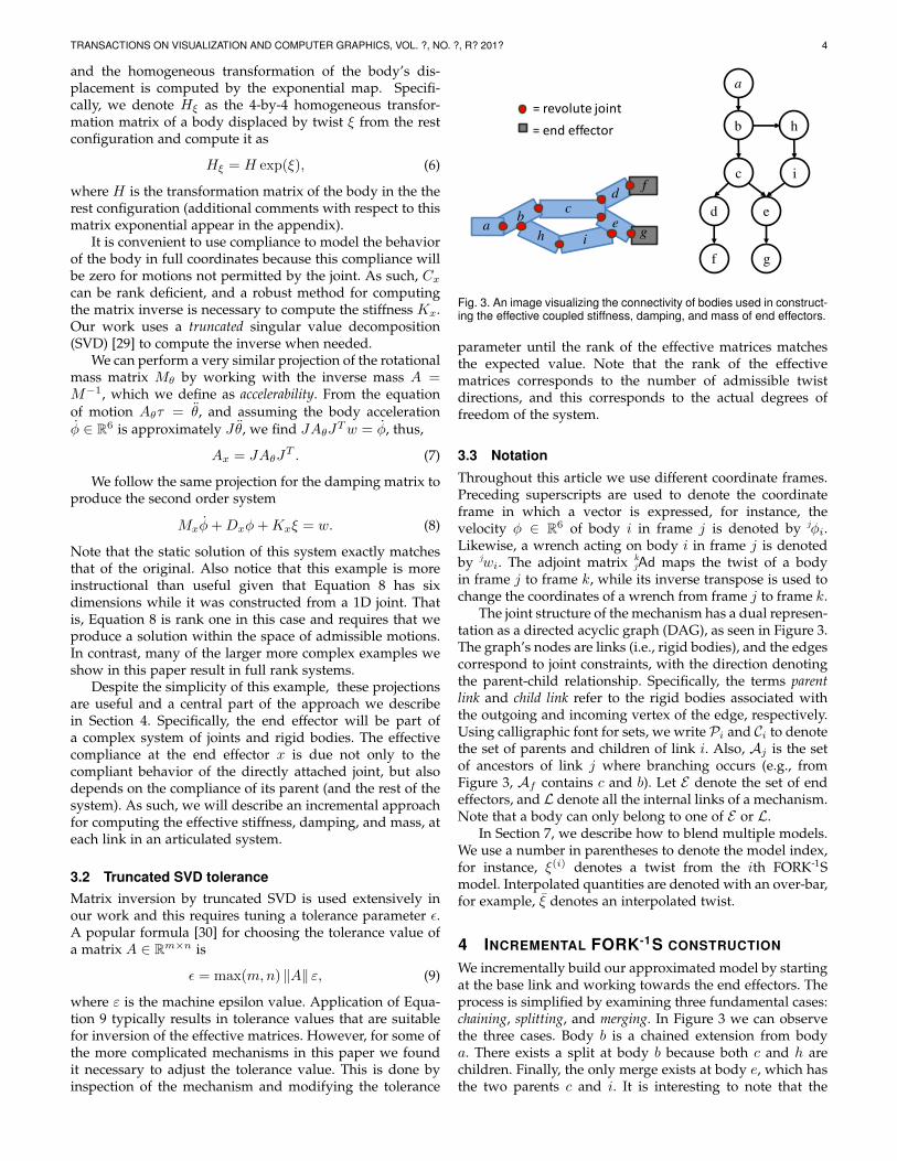
Fig. 3. An image visualizing the connectivity of bodies used in construct-ing the effective coupled stiffness, damping, and mass of end effectors.

parameter until the rank of the effective matrices matchesthe expected value. Note that the rank of the effectivematrices corresponds to the number of admissible twistdirections, and this corresponds to the actual degrees offreedom of the system.

3.3 Notation

Throughout this article we use different coordinate frames.Preceding superscripts are used to denote the coordinateframe in which a vector is expressed, for instance, thevelocity φ ∈ R6 of body i in frame j is denoted by jφi.Likewise, a wrench acting on body i in frame j is denotedby jwi. The adjoint matrix k

jAd maps the twist of a bodyin frame j to frame k, while its inverse transpose is used tochange the coordinates of a wrench from frame j to frame k.

The joint structure of the mechanism has a dual represen-tation as a directed acyclic graph (DAG), as seen in Figure 3.The graph’s nodes are links (i.e., rigid bodies), and the edgescorrespond to joint constraints, with the direction denotingthe parent-child relationship. Specifically, the terms parentlink and child link refer to the rigid bodies associated withthe outgoing and incoming vertex of the edge, respectively.Using calligraphic font for sets, we write Pi and Ci to denotethe set of parents and children of link i. Also, Aj is the setof ancestors of link j where branching occurs (e.g., fromFigure 3, Af contains c and b). Let E denote the set of endeffectors, and L denote all the internal links of a mechanism.Note that a body can only belong to one of E or L.

In Section 7, we describe how to blend multiple models.We use a number in parentheses to denote the model index,for instance, ξ(i) denotes a twist from the ith FORK-1Smodel. Interpolated quantities are denoted with an over-bar,for example, ξ denotes an interpolated twist.

4 INCREMENTAL FORK-1S CONSTRUCTION

We incrementally build our approximated model by startingat the base link and working towards the end effectors. Theprocess is simplified by examining three fundamental cases:chaining, splitting, and merging. In Figure 3 we can observethe three cases. Body b is a chained extension from bodya. There exists a split at body b because both c and h arechildren. Finally, the only merge exists at body e, which hasthe two parents c and i. It is interesting to note that the


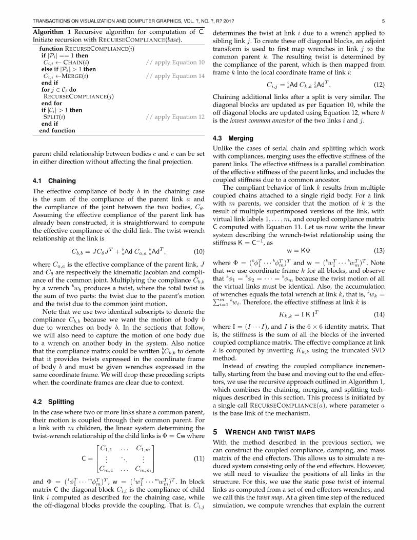
Algorithm 1 Recursive algorithm for computation of C.Initiate recursion with RECURSECOMPLIANCE(base).

function RECURSECOMPLIANCE(i)if |Pi| == 1 thenCi,i ← CHAIN(i) // apply Equation 10

else if |Pi| > 1 thenCi,i ←MERGE(i) // apply Equation 14

end iffor j ∈ Ci doRECURSECOMPLIANCE(j)

end forif |Ci| > 1 thenSPLIT(i) // apply Equation 12

end ifend function

parent child relationship between bodies c and e can be setin either direction without affecting the final projection.

4.1 Chaining

The effective compliance of body b in the chaining caseis the sum of the compliance of the parent link a andthe compliance of the joint between the two bodies, Cθ .Assuming the effective compliance of the parent link hasalready been constructed, it is straightforward to computethe effective compliance of the child link. The twist-wrenchrelationship at the link is

Cb,b = JCθJT + b

aAd Ca,abaAdT , (10)

where Ca,a is the effective compliance of the parent link, Jand Cθ are respectively the kinematic Jacobian and compli-ance of the common joint. Multiplying the compliance Cb,bby a wrench bwb produces a twist, where the total twist isthe sum of two parts: the twist due to the parent’s motionand the twist due to the common joint motion.

Note that we use two identical subscripts to denote thecompliance Cb,b because we want the motion of body bdue to wrenches on body b. In the sections that follow,we will also need to capture the motion of one body dueto a wrench on another body in the system. Also noticethat the compliance matrix could be written b

bCb,b to denotethat it provides twists expressed in the coordinate frameof body b and must be given wrenches expressed in thesame coordinate frame. We will drop these preceding scriptswhen the coordinate frames are clear due to context.

4.2 Splitting

In the case where two or more links share a common parent,their motion is coupled through their common parent. Fora link with m children, the linear system determining thetwist-wrench relationship of the child links is Φ = Cw where

C =

C1,1 . . . C1,m

.... . .

...Cm,1 . . . Cm,m

(11)

and Φ = (1φT1 · · ·mφTm)T , w = (1wT1 · · ·

mwTm)T . In blockmatrix C the diagonal block Ci,i is the compliance of childlink i computed as described for the chaining case, whilethe off-diagonal blocks provide the coupling. That is, Ci,j

determines the twist at link i due to a wrench applied tosibling link j. To create these off diagonal blocks, an adjointtransform is used to first map wrenches in link j to thecommon parent k. The resulting twist is determined bythe compliance of the parent, which is then mapped fromframe k into the local coordinate frame of link i:

Ci,j = ikAd Ck,k

jkAdT . (12)

Chaining additional links after a split is very similar. Thediagonal blocks are updated as per Equation 10, while theoff diagonal blocks are updated using Equation 12, where kis the lowest common ancestor of the two links i and j.

4.3 MergingUnlike the cases of serial chain and splitting which workwith compliances, merging uses the effective stiffness of theparent links. The effective stiffness is a parallel combinationof the effective stiffness of the parent links, and includes thecoupled stiffness due to a common ancestor.

The compliant behavior of link k results from multiplecoupled chains attached to a single rigid body. For a linkwith m parents, we consider that the motion of k is theresult of multiple superimposed versions of the link, withvirtual link labels 1, . . . ,m, and coupled compliance matrixC computed with Equation 11. Let us now write the linearsystem describing the wrench-twist relationship using thestiffness K = C−1, as

w = KΦ (13)

where Φ = (kφT1 · · ·kφTm)T and w = (kwT1 · · ·

kwTm)T . Notethat we use coordinate frame k for all blocks, and observethat kφ1 = kφ2 = · · · = kφm because the twist motion of allthe virtual links must be identical. Also, the accumulationof wrenches equals the total wrench at link k, that is, kwk =∑mi=1

kwi. Therefore, the effective stiffness at link k is

Kk,k = I K IT (14)

where I = (I · · · I), and I is the 6 × 6 identity matrix. Thatis, the stiffness is the sum of all the blocks of the invertedcoupled compliance matrix. The effective compliance at linkk is computed by inverting Kk,k using the truncated SVDmethod.

Instead of creating the coupled compliance incremen-tally, starting from the base and moving out to the end effec-tors, we use the recursive approach outlined in Algorithm 1,which combines the chaining, merging, and splitting tech-niques described in this section. This process is initiated bya single call RECURSECOMPLIANCE(a), where parameter ais the base link of the mechanism.

5 WRENCH AND TWIST MAPS

With the method described in the previous section, wecan construct the coupled compliance, damping, and massmatrix of the end effectors. This allows us to simulate a re-duced system consisting only of the end effectors. However,we still need to visualize the positions of all links in thestructure. For this, we use the static pose twist of internallinks as computed from a set of end effectors wrenches, andwe call this the twist map. At a given time step of the reducedsimulation, we compute wrenches that explain the current


state, i.e., current twists, thus producing a compatible posefor the internal links.

In order to compute the twist map, we first describethe construction of a wrench map that distributes wrenchesapplied at the end effectors to the internal links. These mapsare built incrementally. Our algorithm starts at each endeffector and traverses the DAG of the mechanism in reverseorder. First, a local wrench map is found that distributeswrenches from child links to their parents. Then, a globalwrench map is computed by a compound matrix transformalong the kinematic chain.

5.1 Local wrench mapGiven the wrench at link k, the local wrench map may beused to compute the wrenches distributed amongst its par-ent links. Naively, we could simply divide the wrench by thenumber of parent links and compute the wrench to transferto the parent links using the appropriate adjoint transforms.However, this division of force will not be correct becausethe wrenches transmitted down different chains will dependon the effective compliance of each chain. Thus we constructa linear system to ensure that wrenches are distributed in aplausible manner that respects the internal joint constraintsand compliances.

Note that the sum of the wrenches at the parent linksmust equal the wrench applied at the child link k. That is,

kwk =∑i∈Pk

ikAdT iwi. (15)

Consider the case of m superimposed virtual links thatwas presented in Section 4.3. We can write the followingconstrained linear system to determine the distribution ofwrenches on the different chains:[

C IT

I 0

] [wλ

]=

[0

kwk

]. (16)

The constraint here is the same as Equation 15, exceptthat all quantities are represented in frame k, and thus theadjoints are 6 × 6 identity matrices, i.e., I w = kwk. Tocompute a local wrench map that takes the wrench fromk and divides it among its parents 1, . . . ,m, we invert thesystem above, replacing the right hand side by a blockcolumn matrix that will provide the desired vector whenright multiplied by kwk. That is,

1Wk

...mWk

∗

=

[C IT

I 0

]−1 [0I

]. (17)

This gives us a block column vector containing the wrenchmap for each parent link, with a block ∗ due to the Lagrangemultipliers that we can ignore. Note that forming the lefthand side blocks iWk requires computing the inverse of asystem that may be rank deficient due to the coupled com-pliance. Again, we use a truncated SVD in its computation.

Finally, while these wrench maps only consider thedifficult case of merging (multiple parents) by using super-imposed virtual parent links, the transmission of wrenchesalong simple serial chains is easy. It simply involves achange of coordinates with an adjoint inverse transpose. For

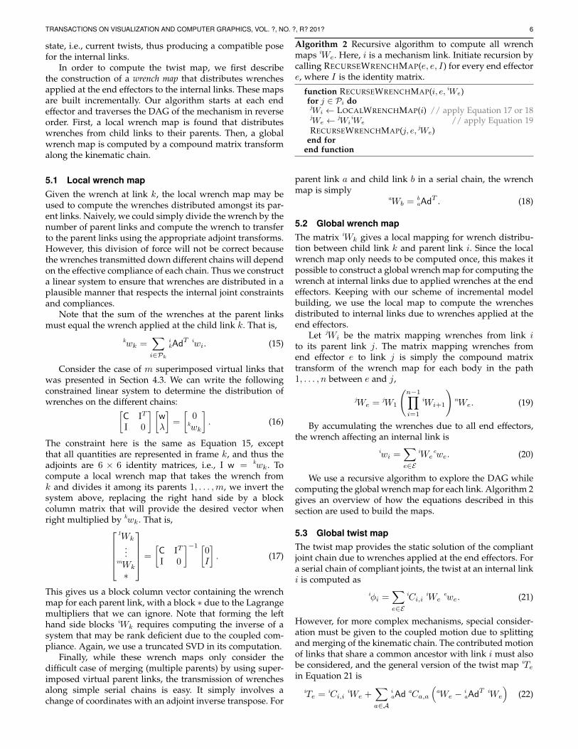
Algorithm 2 Recursive algorithm to compute all wrenchmaps iWe. Here, i is a mechanism link. Initiate recursion bycalling RECURSEWRENCHMAP(e, e, I) for every end effectore, where I is the identity matrix.

function RECURSEWRENCHMAP(i, e, iWe)for j ∈ Pi dojWi ← LOCALWRENCHMAP(i) // apply Equation 17 or 18jWe ← jWi

iWe // apply Equation 19RECURSEWRENCHMAP(j, e, jWe)

end forend function

parent link a and child link b in a serial chain, the wrenchmap is simply

aWb = baAdT . (18)

5.2 Global wrench mapThe matrix iWk gives a local mapping for wrench distribu-tion between child link k and parent link i. Since the localwrench map only needs to be computed once, this makes itpossible to construct a global wrench map for computing thewrench at internal links due to applied wrenches at the endeffectors. Keeping with our scheme of incremental modelbuilding, we use the local map to compute the wrenchesdistributed to internal links due to wrenches applied at theend effectors.

Let jWi be the matrix mapping wrenches from link ito its parent link j. The matrix mapping wrenches fromend effector e to link j is simply the compound matrixtransform of the wrench map for each body in the path1, . . . , n between e and j,

jWe = jW1

(n−1∏i=1

iWi+1

)nWe. (19)

By accumulating the wrenches due to all end effectors,the wrench affecting an internal link is

iwi =∑e∈E

iWeewe. (20)

We use a recursive algorithm to explore the DAG whilecomputing the global wrench map for each link. Algorithm 2gives an overview of how the equations described in thissection are used to build the maps.

5.3 Global twist mapThe twist map provides the static solution of the compliantjoint chain due to wrenches applied at the end effectors. Fora serial chain of compliant joints, the twist at an internal linki is computed as

iφi =∑e∈E

iCi,iiWe

ewe. (21)

However, for more complex mechanisms, special consider-ation must be given to the coupled motion due to splittingand merging of the kinematic chain. The contributed motionof links that share a common ancestor with link i must alsobe considered, and the general version of the twist map iTein Equation 21 is

iTe = iCi,iiWe +

∑a∈A

iaAd aCa,a

(aWe − i

aAdT iWe

)(22)


and iφi =∑e∈E

iTeewe. The twist has a component due to

the wrench arriving from each ancestor, but also experiencesmotion due to that of its ancestors influenced by end effectorwrenches. The subtraction in the last term ensures that wedo not include the motion of the ancestor induced by thewrench transmitted through the chain containing link i,because it is already accounted for in the first term.

6 DYNAMIC SIMULATION

We simulate the reduced dynamic system using a backwardEuler formulation [31]. As such, we have a system matrix ofthe form

A = M− h2K− hD. (23)

To solve this system with frictional contacts, we use an iter-ative projected Gauss-Seidel solver similar to that describedby Erleben [32]. This involves a Schur complement of theform GTA−1G, where G is the Jacobian for the contact andfriction constraints. We note that it is only necessary toinvert the system matrix once, and reuse this small denseinverse system for the duration of the simulation.

The solution to the reduced dynamic system only pro-vides the positions (twists, ξ) and velocities of the endeffectors links. Internal links are updated using the twists ofthe end effectors. Specifically, we compute equivalent staticend effector wrenches as w = Kξ, and from these computethe configuration of internal links using the twist map inEquation 22.

6.1 Free-body base linkFor simplicity, the discussion above has let the body frameof the base link be fixed in the world. To extend the reducedmodel to allow for motion at the base, we integrate a secondequation of motion for a rigid body representing the base.We set the base mass and inertia matrix to be that of theentire structure in the rest pose. The motion of the base isdriven by gravity, but also by the net external wrenchesapplied at the end effectors. While the coupled equationsof motion could be derived from the Lagrangian, we onlycouple the base and end-effector models through externalforces, and assume that the omitted terms such as Coriolisforces are negligible when the base has large mass andis moving slowly. In this case, the contact and frictionalconstraints must be modified to use the combined velocityof the base link bφb and velocity of the end effector link kφkin contact frame c, cφk+b = c

kAd kφk + cbAd bφb.

7 COMBINING MULTIPLE FORK-1S MODELS

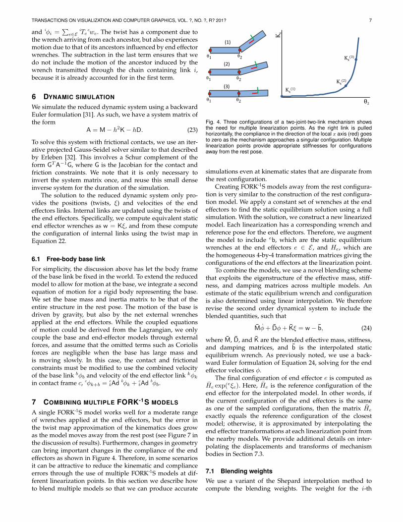
A single FORK-1S model works well for a moderate rangeof wrenches applied at the end effectors, but the error inthe twist map approximation of the kinematics does growas the model moves away from the rest post (see Figure 7 inthe discussion of results). Furthermore, changes in geometrycan bring important changes in the compliance of the endeffectors as shown in Figure 4. Therefore, in some scenariosit can be attractive to reduce the kinematic and complianceerrors through the use of multiple FORK-1S models at dif-ferent linearization points. In this section we describe howto blend multiple models so that we can produce accurate

Kx

θ2

(1)

(2)

(3)Kx

(1)

Kx(2)

Kx(3)

θ2

θ1 θ2

θ2θ1

θ1

Fig. 4. Three configurations of a two-joint-two-link mechanism showsthe need for multiple linearization points. As the right link is pulledhorizontally, the compliance in the direction of the local x axis (red) goesto zero as the mechanism approaches a singular configuration. Multiplelinearization points provide appropriate stiffnesses for configurationsaway from the rest pose.

simulations even at kinematic states that are disparate fromthe rest configuration.

Creating FORK-1S models away from the rest configura-tion is very similar to the construction of the rest configura-tion model. We apply a constant set of wrenches at the endeffectors to find the static equilibrium solution using a fullsimulation. With the solution, we construct a new linearizedmodel. Each linearization has a corresponding wrench andreference pose for the end effectors. Therefore, we augmentthe model to include eb, which are the static equilibriumwrenches at the end effectors e ∈ E , and He, which arethe homogeneous 4-by-4 transformation matrices giving theconfigurations of the end effectors at the linearization point.

To combine the models, we use a novel blending schemethat exploits the eigenstructure of the effective mass, stiff-ness, and damping matrices across multiple models. Anestimate of the static equilibrium wrench and configurationis also determined using linear interpolation. We thereforerevise the second order dynamical system to include theblended quantities, such that

Mφ+ Dφ+ Kξ = w − b, (24)

where M, D, and K are the blended effective mass, stiffness,and damping matrices, and b is the interpolated staticequilibrium wrench. As previously noted, we use a back-ward Euler formulation of Equation 24, solving for the endeffector velocities φ.

The final configuration of end effector e is computed asHe exp(eξe). Here, He is the reference configuration of theend effector for the interpolated model. In other words, ifthe current configuration of the end effectors is the sameas one of the sampled configurations, then the matrix He

exactly equals the reference configuration of the closestmodel; otherwise, it is approximated by interpolating theend effector transformations at each linearization point fromthe nearby models. We provide additional details on inter-polating the displacements and transforms of mechanismbodies in Section 7.3.

7.1 Blending weightsWe use a variant of the Shepard interpolation method tocompute the blending weights. The weight for the i-th


Algorithm 3 Blend matrices with rank-1 updates. Weightsα1...k interpolate the eigendecomposition of matricesA(1...k). Function RANK(A, ε) computes the rank of A withtolerance ε, and EIG(A) returns the eigendecomposition.

function BLENDRANK1(A(1...k), α1...k, ε)A← 0r = RANK(A(1), ε)Q(1),Λ(1) ← EIG(A(1)) // Note that this is pre-computedfor j ∈ 1 . . . r doq ← α1Q

(1)j

λ← α1Λ(1)jj

for i ∈ (2 . . . k) doQ(i),Λ(i) ← EIG(A(i)) // Note that this is pre-computedq ← vector in Q(i)

1...r most similar to Q(1)j

λ← diagonal entry in Λ(i) corresponding to qq ← q′ + αiqλ← λ+ αiλ

end forq ← q

‖q‖A← A+ λ qqT

end forreturn Aend function

nearby model is

αi =1

s

(∑e∈E ‖ξe − ξ

(i)e ‖)−p

, (25)

where s is a normalization factor such that the sum of allαi equals 1. For the results obtained in this paper, we usep = 2. The distance to the nearby model is computed usingthe current end effector displacement ξe and the end effectordisplacement at the sample configuration ξ(i)e relative to thebase link. We mix linear and angular components of thetwist vectors by scaling factors 1

r and 1π respectively, where

r is the bounding sphere radius of the mechanism. Thesescaling factors are omitted from Equation 25 for brevity.

7.2 Interpolating the effective matricesThe first step in performing simulation by Equation 24 is tocompute the interpolated effective matrices. As opposed tosimply blending matrix elements, we use the eigenstructureof each matrix so that the effective mass, stiffness, anddamping of end effectors can rotate in a smooth manneracross the configuration space. Consider the example inFigure 4. As the second joint rotates, the contribution of thecompliance of the first joint will be in a different direction inthe local coordinate frame. By interpolating the eigenvectordirections we can produce a plausible end effector compli-ance.

We group the eigenvectors of different matrices accord-ing to their similarity computed by a dot product. Thegrouping of eigenvectors across different models is straight-forward when the linearized models are not too far fromone another in the configuration space. We pre-compute theeigendecomposition of the effective matrices and store theeigenvectors and eigenvalues with each model.

At run time, we interpolate the eigenvectors and corre-sponding eigenvalues using the blending weights, and thenassemble the blended matrix as a sum of rank-1 matrices.These are formed by the outer-products of the interpolated

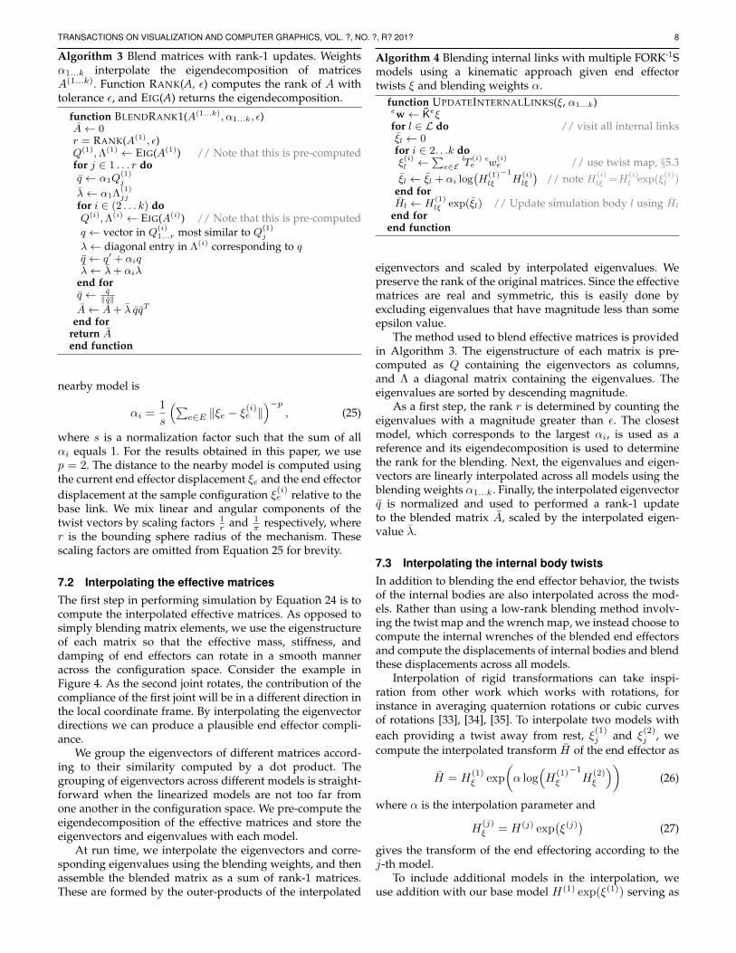
Algorithm 4 Blending internal links with multiple FORK-1Smodels using a kinematic approach given end effectortwists ξ and blending weights α.

function UPDATEINTERNALLINKS(ξ, α1...k)ew← Keξfor l ∈ L do // visit all internal linksξl ← 0for i ∈ 2. . .k doξ

(i)l ←

∑e∈E

lT(i)e

ew(i)e // use twist map, §5.3

ξl ← ξl + αi log(H

(1)lξ

−1H

(i)lξ

)// note H(i)

lξ =H(i)l exp(ξ

(i)l )

end forHl ← H

(1)lξ exp(ξl) // Update simulation body l using Hl

end forend function

eigenvectors and scaled by interpolated eigenvalues. Wepreserve the rank of the original matrices. Since the effectivematrices are real and symmetric, this is easily done byexcluding eigenvalues that have magnitude less than someepsilon value.

The method used to blend effective matrices is providedin Algorithm 3. The eigenstructure of each matrix is pre-computed as Q containing the eigenvectors as columns,and Λ a diagonal matrix containing the eigenvalues. Theeigenvalues are sorted by descending magnitude.

As a first step, the rank r is determined by counting theeigenvalues with a magnitude greater than ε. The closestmodel, which corresponds to the largest αi, is used as areference and its eigendecomposition is used to determinethe rank for the blending. Next, the eigenvalues and eigen-vectors are linearly interpolated across all models using theblending weights α1...k. Finally, the interpolated eigenvectorq is normalized and used to performed a rank-1 updateto the blended matrix A, scaled by the interpolated eigen-value λ.

7.3 Interpolating the internal body twistsIn addition to blending the end effector behavior, the twistsof the internal bodies are also interpolated across the mod-els. Rather than using a low-rank blending method involv-ing the twist map and the wrench map, we instead choose tocompute the internal wrenches of the blended end effectorsand compute the displacements of internal bodies and blendthese displacements across all models.

Interpolation of rigid transformations can take inspi-ration from other work which works with rotations, forinstance in averaging quaternion rotations or cubic curvesof rotations [33], [34], [35]. To interpolate two models witheach providing a twist away from rest, ξ(1)j and ξ

(2)j , we

compute the interpolated transform H of the end effector as

H = H(1)ξ exp

(α log

(H

(1)ξ

−1H

(2)ξ

))(26)

where α is the interpolation parameter and

H(j)ξ = H(j) exp

(ξ(j)

)(27)

gives the transform of the end effectoring according to thej-th model.

To include additional models in the interpolation, weuse addition with our base model H(1) exp(ξ(1)) serving as


Algorithm 5 The simulation algorithm for blended FORK-1Scombines methods for interpolating the effective matricesand displacements of the internal bodies.

function BLENDEDSIMULATIONCompute blending weights α1...k // see Equation 25M← BLENDRANK1(M(1...k), α1...k, ε)K← BLENDRANK1(K(1...k), α1...k, ε)D← BLENDRANK1(D(1...k), α1...k, ε)for e ∈ E doebe ←

∑ki=1 αi

eb(i)e // static equilibrium wrench

He ← H(1)e exp

(∑ki=2 αi log(H

(1)e

−1H

(i)e ))

// ref. config.end forξ ← STEPENDEFFECTORDYNAMICS // solve Equation 24UPDATEINTERNALLINKS(ξ, α1...k) // see Algorithm 4

end function

the linearization point for other models. The observation isthat this works well as long as the error for both our basemodel and the other models are close enough. The otherobservation is that while order is important when chainingmultiplications, by doing interpolation with addition insidethe exponential we avoid the order dependence of matrixmultiplication. Specifically,

H = H(1) exp( k∑j=2

αj log(H(1)−1H(j))). (28)

Algorithm 4 outlines the method used to perform kine-matic blending of the internal links. Much as in the singlemodel approach, the end effector wrenches ew are estimatedas the end effector displacements eξ transformed by theinterpolated stiffness. For each model, the displacementcontributed by each end effector is computed using the twistmap lT

(i)e , which is specific to the link and the model. This

is then used to update the interpolated displacement ξl oflink l using Equation 28. Note that our implementation ofthe Algorithm 4 is parallelized, per link, across the models.

7.4 Blended FORK-1S simulationThe procedure for dynamical simulation of the blendedmodel is outlined in Algorithm 5. The first step is to de-termine the blending weights based on the current displace-ments of the effectors. We then compute the interpolatedmass, stiffness, and damping matrices, along with the staticequilibrium wrench and reference configuration for eachend effector. With the blended model, we then step thesimulation of the end effectors and update positions ofinternal links.

7.5 Model selectionNon-parametric regression methods, such as the k-nearestneighbors (k-NN) algorithm, seem well-suited for ourblending approach. However, this requires selecting a subsetof the sampled models and interpolating across them. Wehave observed that excluding models from blending canproduce popping artifacts in the motion of the internallinks. Therefore, we choose to perform blending across allof the sampled models. While blending across all models iswasteful, we recognize that a good avenue of future researchwould be to group models into well-behaved subsets and to

build a graph of these subsets that can be walked at run-time.

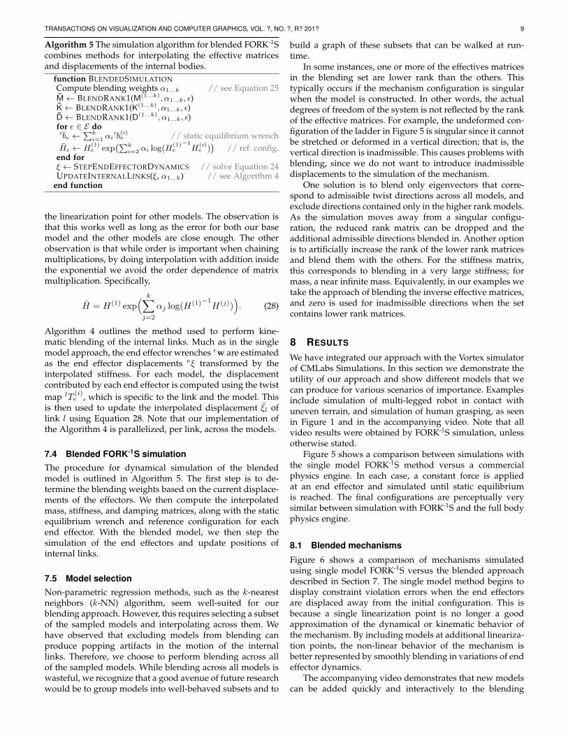
In some instances, one or more of the effectives matricesin the blending set are lower rank than the others. Thistypically occurs if the mechanism configuration is singularwhen the model is constructed. In other words, the actualdegrees of freedom of the system is not reflected by the rankof the effective matrices. For example, the undeformed con-figuration of the ladder in Figure 5 is singular since it cannotbe stretched or deformed in a vertical direction; that is, thevertical direction is inadmissible. This causes problems withblending, since we do not want to introduce inadmissibledisplacements to the simulation of the mechanism.

One solution is to blend only eigenvectors that corre-spond to admissible twist directions across all models, andexclude directions contained only in the higher rank models.As the simulation moves away from a singular configu-ration, the reduced rank matrix can be dropped and theadditional admissible directions blended in. Another optionis to artificially increase the rank of the lower rank matricesand blend them with the others. For the stiffness matrix,this corresponds to blending in a very large stiffness; formass, a near infinite mass. Equivalently, in our examples wetake the approach of blending the inverse effective matrices,and zero is used for inadmissible directions when the setcontains lower rank matrices.

8 RESULTS

We have integrated our approach with the Vortex simulatorof CMLabs Simulations. In this section we demonstrate theutility of our approach and show different models that wecan produce for various scenarios of importance. Examplesinclude simulation of multi-legged robot in contact withuneven terrain, and simulation of human grasping, as seenin Figure 1 and in the accompanying video. Note that allvideo results were obtained by FORK-1S simulation, unlessotherwise stated.

Figure 5 shows a comparison between simulations withthe single model FORK-1S method versus a commercialphysics engine. In each case, a constant force is appliedat an end effector and simulated until static equilibriumis reached. The final configurations are perceptually verysimilar between simulation with FORK-1S and the full bodyphysics engine.

8.1 Blended mechanisms

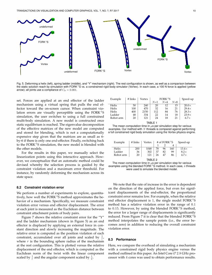
Figure 6 shows a comparison of mechanisms simulatedusing single model FORK-1S versus the blended approachdescribed in Section 7. The single model method begins todisplay constraint violation errors when the end effectorsare displaced away from the initial configuration. This isbecause a single linearization point is no longer a goodapproximation of the dynamical or kinematic behavior ofthe mechanism. By including models at additional lineariza-tion points, the non-linear behavior of the mechanism isbetter represented by smoothly blending in variations of endeffector dynamics.

The accompanying video demonstrates that new modelscan be added quickly and interactively to the blending


FORK-1S

FORK-1S

FORK-1S

Vortex

undeformed

Vortex Vortex undeformed

undeformed

Fig. 5. Deforming a helix (left), spring ladder (middle), and “Y” mechanism (right). The rest configuration is shown, as well as a comparison betweenthe static solution reach by simulation with FORK-1S vs. a constrained rigid body simulator (Vortex). In each case, a 100 N force is applied (yellowarrow); all joints use a compliance of Cθ = 0.001.

set. Forces are applied at an end effector of the laddermechanism using a virtual spring that pulls the end ef-fector toward the on-screen cursor. When constraint vio-lation errors are visually perceptible using the FORK-1Ssimulation, the user switches to using a full constrainedmulti-body simulation. A new model is constructed oncestatic equilibrium is reached. The eigenvalue decompositionof the effective matrices of the new model are computedand stored for blending, which is not a computationallyexpensive step given that the matrices are as small as 6-by-6 if there is only one end-effector. Finally, switching backto the FORK-1S simulation, the new model is blended withthe other models.

For the results in this paper, we manually select thelinearization points using this interactive approach. How-ever, we conceptualize that an automatic method could bedevised whereby the selection process is guided by theconstraint violation and a maximum error threshold. Forinstance, by randomly deforming the mechanism across itsstate space.

8.2 Constraint violation error

We perform a number of experiments to explore, quantita-tively, how well the FORK-1S method approximates the be-havior of a mechanism. Specifically, we measure constraintviolation error versus end effector displacement. The errorat each joint is measured as the Euclidean distance betweenconstraint attachment points of body pairs.

Figure 7 shows the relative constraint error for the “Y”and the ladder mechanism (shown in Figure 5) as an endeffector is displaced by applying an external force in con-stant direction and slowly increasing the magnitude. Therelative error is computed as the position violation of eachconstraint, accumulated over all joints and scaled by 1

r ,where r is the bounding sphere radius of the mechanismat the rest configuration. This is plotted versus the relativedisplacement of the end effector, which is computed as theEuclidean norm of the twist with the linear componentscaled by 1

r and the angular component scaled by 1π .

Example # links Vortex FORK-1S Speed-upN=1 N=4 N=8

Helix 50 240 20 12 15 20.0×Helix 100 470 32 16 21 29.4×Helix 400 2150 112 84 76 28.3×Ladder 48 334 22 14 18 23.9×Robot arm 20 121 24 18 21 6.7×

TABLE 1The mean computation time in µs per simulation step for various

examples. Our method with N threads is compared against performinga full constrained rigid body simulation using the Vortex physics engine.

Example # links Vortex # of FORK-1S Speed-up1 2 4

Helix 200 1048 78 96 160 13.4×Ladder 36 302 37 82 99 8.2×Robot arm 20 121 26 47 86 4.7×

TABLE 2The mean computation time in µs per simulation step for various

examples using the blended FORK-1S method. In each case, 4 threadswere used to simulate the blended model.

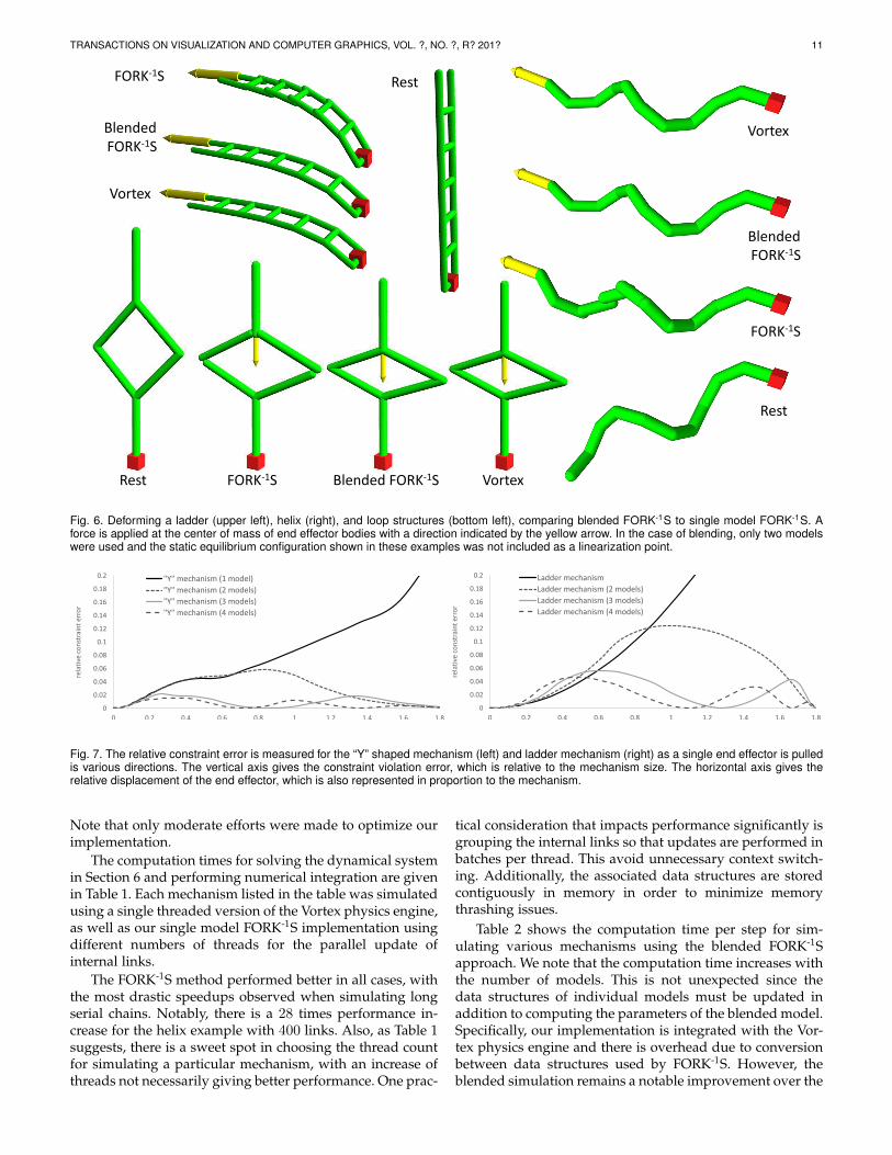
We note that the rate of increase in the error is dependenton the direction of the applied force, but even for signif-icant displacements of the end-effector, the proportionalconstraint error remains low. For example, when the relativeend effector displacement is 1, the single model FORK-1Smethod has a relative violation error in the range of 0.1to 0.15. However, by using the blended FORK-1S method,the error for a larger range of displacements is significantlyreduced. From Figure 7 it is clear that the blended FORK-1Smethod interpolates the sample points (i.e., the error be-comes zero) in addition to reducing the overall constraintviolation error.

8.3 Performance

Here, we compare the overhead of simulating a mechanismwith a constrained rigid body physics engine versus themethod outlined in this paper. An Intel Core i7 2.8 GHz pro-cessor with 4 cores was used to obtain performance results.


RestFORK-1S

Blended FORK-1S

Vortex

Vortex

Blended FORK-1S

FORK-1S

Rest

FORK-1S Blended FORK-1S VortexRest

Fig. 6. Deforming a ladder (upper left), helix (right), and loop structures (bottom left), comparing blended FORK-1S to single model FORK-1S. Aforce is applied at the center of mass of end effector bodies with a direction indicated by the yellow arrow. In the case of blending, only two modelswere used and the static equilibrium configuration shown in these examples was not included as a linearization point.

0

0.02

0.04

0.06

0.08

0.1

0.12

0.14

0.16

0.18

0.2

0 0.2 0.4 0.6 0.8 1 1.2 1.4 1.6 1.8

rela

tive

co

nst

rain

t er

ror

relative displacement |K-1w|

"Y" mechanism (1 model)

"Y" mechanism (2 models)



0

0.02

0.04

0.06

0.08

0.1

0.12

0.14

0.16

0.18

0.2

0 0.2 0.4 0.6 0.8 1 1.2 1.4 1.6 1.8

rela

tive

co

nst

rain

t er

ror

relative displacement |K-1w|

Ladder mechanism

Ladder mechanism (2 models)



Fig. 7. The relative constraint error is measured for the “Y” shaped mechanism (left) and ladder mechanism (right) as a single end effector is pulledis various directions. The vertical axis gives the constraint violation error, which is relative to the mechanism size. The horizontal axis gives therelative displacement of the end effector, which is also represented in proportion to the mechanism.

Note that only moderate efforts were made to optimize ourimplementation.

The computation times for solving the dynamical systemin Section 6 and performing numerical integration are givenin Table 1. Each mechanism listed in the table was simulatedusing a single threaded version of the Vortex physics engine,as well as our single model FORK-1S implementation usingdifferent numbers of threads for the parallel update ofinternal links.

The FORK-1S method performed better in all cases, withthe most drastic speedups observed when simulating longserial chains. Notably, there is a 28 times performance in-crease for the helix example with 400 links. Also, as Table 1suggests, there is a sweet spot in choosing the thread countfor simulating a particular mechanism, with an increase ofthreads not necessarily giving better performance. One prac-

tical consideration that impacts performance significantly isgrouping the internal links so that updates are performed inbatches per thread. This avoid unnecessary context switch-ing. Additionally, the associated data structures are storedcontiguously in memory in order to minimize memorythrashing issues.

Table 2 shows the computation time per step for sim-ulating various mechanisms using the blended FORK-1Sapproach. We note that the computation time increases withthe number of models. This is not unexpected since thedata structures of individual models must be updated inaddition to computing the parameters of the blended model.Specifically, our implementation is integrated with the Vor-tex physics engine and there is overhead due to conversionbetween data structures used by FORK-1S. However, theblended simulation remains a notable improvement over the


full constrained rigid body simulation. Also, Equation 26is used to update the reference configuration of the endeffectors as well as the configuration of the internal links.Conversion of the homogeneous transform matrix usingthe exponential map becomes a bottle neck is this case,and further performance improvement could be realized byoptimizing our implementation of this function.

8.4 Discussion and limitations

Interior body reconstructions have constraint errors whenlarge external forces are applied at the end effectors of asimulation with just a single FORK-1S model. Therefore oneof our contributions with this work is to introduce modelsat additional linearization points and blend their behavioras the system is pulled from its rest state.

Although the added models extend the range of motionfor a mechanism, geometric limits of the internal joints arenot necessarily well approximated by our method. Adap-tively stiffening the system may help in these situations,become stiffer as singular and joint limit configurations areapproached. This strategy could also be used to avoid stateswhere joint constraint errors appear. We leave joint limitsand additional non-linear compliance scaling for futurework.

It is also possible to make small modifications to the ge-ometry to correct errors at the expense of letting rigid linksdeform, and such strategies have been used in repairing footskate [36] and length changes are often not perceived [37].Errors can be fixed by allowing rigid bodies to stretch, butthere is a limit to how large external forces can grow beforegeometry modifications are visible.

We note that the behavior of the reduced model candiffer from the full model. In general, we observe the re-duced systems to be slightly stiffer than their fully simulatedsystems. This is not surprising, and we believe this occursnaturally due to the lower number of degrees of freedomand the linearization we impose. Higher levels of dampingseen in the reduced system can be explained by our im-plicit integration, while Vortex uses a symplectic integrationscheme.

The construction process assumes that we can walk froma base node in the graph to all end effectors. When there areloop closures between two end effectors that are on the farside of the graph from the base, the incremental algorithmwill not find them. An alternative projection technique isnecessary in this case.

9 CONCLUSION

First order reduced models of compliant mechanisms pro-vide a fast alternative to simulating virtual humans androbots. By focusing only on the end effectors, the simulationonly needs to solve a small dense system while the fullstate of the non-reduced mechanism can be computed inparallel. Using the exponential map to compute the state ofthe internal links produces a desirable behavior with littleseparation at joints for a good range of interaction forces.Our method deals with loops in the constraints, and permitsdifferent levels of physics fidelity by adjusting the numberof end effectors included in the reduced model. Finally, with

the method we present for blending multiple linearizationpoints we can accurately simulate structures over a widerrange of simulation states.

FORK-1S provide an important new approach among alarge spectrum of techniques important for the creation ofinteractive and immerse virtual environments. We believeit will be a useful tool for improving industrial trainingsimulations and physics-based character animation.

9.1 Future WorkA number of avenues of future work are discussed inSection 8.4. We also intend to investigate various methodsfor controlling end effector motion. This is useful for manyapplications, such as manipulation tasks in character ani-mation and robotics simulation. Online control for dexter-ous manipulation tasks has been successfully demonstratedusing PD servo control [38]. We believe a similar controlframework could be achieved using FORK-1S, for example,by modulating the static equilibrium wrench to drive thegripper towards a set point posture rather than interpolatingthe value of be across the models. Similarly, our reducedcompliant model could be used to perform short-horizonmotion planning using model predictive control (MPC), forinstance, in combination with the technique described byKumar et al. [39]. We believe that reduced models for MPCare an important avenue of future research.

APPENDIX - RIGID BODY KINEMATICS

Any rigid motion from one position to another may bedescribed as a screw motion. That is, there exists a coordinateframe in which the motion consists of a translation alongan axis combined with a rotation about the same axis. Thetime derivative of a screw motion is a twist consisting ofthe linear velocity v ∈ R3 and angular velocity ω ∈ R3.Since much of this paper concerns statics, and because itis convenient to write rigid displacements (screws) in bodycoordinate frames, we abuse the term twist for these smalldisplacements ξ. We use φ and the term velocity to write theequations of motion and specifically use the body velocity asdefined by Murray et al. [28]. Analogous to a twist, a wrenchw ∈ R6 is a generalized force consisting of a linear forcef ∈ R3 and a rotational torque τ ∈ R3. Following Murray etal., we pack twist and wrench vectors with linear parts ontop and angular parts on the bottom, i.e., φ = (vTωT )T andw = (fT τT )T .

Twists and wrenches transform to different coordinateframes using the adjoint matrix Ad ∈ R6×6. To transformtwists from coordinate frame a to coordinate frame b, wedirectly use

baAd =

[baR

bpabaR

0 baR

], (29)

where baR ∈ SO(3) is the rotation matrix from frame a

to b, the origin of coordinate frame a in coordinates offrame b is bpa, and ˆ is the cross product operator. Thatis, aφ in frame b is computed as bφ = b

aAdaφ. The inversetranspose of the adjoint is used to transform a wrenchbetween coordinate frames, bw = b

aAd−T aw. Finally, we usethe exponential map eφ : R6 → SE(3) on a twist to computethe relative rigid motion as a homogeneous transformation


matrix using formulas given by Murray et al. [28]. Here,we follow Murray et al. where the hat notation φ denotesa repacking of the 6 components of a twist into a 4-by-4matrix. However, throughout this paper we omit the hatnotation and let it be implicitly clear from context that theexponential of a twist is indeed the matrix exponential.

ACKNOWLEDGMENTS

We thank the anonymous reviewers for their suggestions forimproving the paper. This work was supported by fundingfrom NSERC, CFI, MITACS, CINQ, and GRAND NCE.

REFERENCES

[1] S. Andrews, M. Teichmann, and P. G. Kry, “FORK-1S: Interactivecompliant mechanisms with parallel state computation,” inProceedings of the 18th Meeting of the ACM SIGGRAPH Symp. onInteractive 3D Graphics and Games, ser. I3D ’14, 2014, pp. 7–14.[Online]. Available: http://doi.acm.org/10.1145/2556700.2556717

[2] A. Nealen, M. Muller, R. Keiser, E. Boxerman, and M. Carlson,“Physically based deformable models in computer graphics,”Computer Graphics Forum, vol. 25, no. 4, pp. 809–836, 2006.

[3] M. Nesme, P. G. Kry, L. Jerabkova, and F. Faure, “Preservingtopology and elasticity for embedded deformable models,” ACMTrans. on Graphics, vol. 28, no. 3, p. 52, 2009.

[4] J. Barbic and Y. Zhao, “Real-time large-deformation substructur-ing,” ACM Trans. on Graphics, vol. 30, no. 4, pp. 91:1–91:8, Jul. 2011.[Online]. Available: http://doi.acm.org/10.1145/2010324.1964986

[5] T. Kim and D. James, “Physics-based character skinning usingmultidomain subspace deformations,” IEEE Trans. on Visualizationand Computer Graphics, vol. 18, no. 8, pp. 1228–1240, 2012.

[6] D. Harmon and D. Zorin, “Subspace integration with localdeformations,” ACM Trans. on Graphics, vol. 32, no. 4, pp.107:1–107:10, 2013. [Online]. Available: http://doi.acm.org/10.1145/2461912.2461922

[7] C. Duriez, F. Dubois, A. Kheddar, and C. Andriot, “Realistic hapticrendering of interacting deformable objects in virtual environ-ments,” IEEE Trans. on Visualization and Computer Graphics, vol. 12,no. 1, pp. 36–47, 2006.

[8] E. G. Parker and J. F. O’Brien, “Real-time deformation andfracture in a game environment,” in Proc. of the ACMSIGGRAPH/Eurographics Symp. on Comp. Anim., 2009, pp. 165–175.[Online]. Available: http://doi.acm.org/10.1145/1599470.1599492

[9] K. Yamane and Y. Nakamura, “Stable penalty-based model offrictional contacts,” in Proc. of IEEE International Conference onRobotics and Automation, 2006, pp. 1904–1909.

[10] J. Allard, F. Faure, H. Courtecuisse, F. Falipou, C. Duriez, and P. G.Kry, “Volume contact constraints at arbitrary resolution,” ACMTrans. on Graphics, vol. 29, no. 4, p. 82, 2010.

[11] C. O’Sullivan and J. Dingliana, “Collisions and perception,” ACMTrans. on Graphics, vol. 20, no. 3, pp. 151–168, 2001. [Online].Available: http://doi.acm.org/10.1145/501786.501788

[12] D. Baraff, “Linear-time dynamics using lagrange multipliers,”in Proc. of the 23rd annual conference on Computer graphicsand interactive techniques, 1996, pp. 137–146. [Online]. Available:http://doi.acm.org/10.1145/237170.237226

[13] U. M. Ascher and L. R. Petzold, Computer Methods for OrdinaryDifferential Equations and Differential-Algebraic Equations, 1st ed.Philadelphia, PA, USA: Society for Industrial and Applied Mathe-matics, 1998.

[14] U. Ascher and P. Lin, “Sequential regularization methods forsimulating mechanical systems with many closed loops,” SIAMJournal on Scientific Computing, vol. 21, no. 4, pp. 1244–1262, 1999.

[15] F. Faure, “Fast iterative refinement of articulated solid dynamics,”IEEE Trans. on Visualization and Computer Graphics, vol. 5, no. 3, pp.268–276, 1999.

[16] R. Tomcin, D. Sibbing, and L. Kobbelt, “Efficient enforcement ofhard articulation constraints in the presence of closed loops andcontacts,” in Computer Graphics Forum, vol. 33, no. 2. Wiley OnlineLibrary, 2014, pp. 235–244.

[17] R. Featherstone and D. Orin, “Robot dynamics: equations andalgorithms,” Proc. of IEEE International Conference on Robotics andAutomation, vol. 1, pp. 826–834, 2000.

[18] R. Featherstone, Rigid Body Dynamics Algorithms. New York:Springer, 2008.

[19] R. M. Mukherjee and K. S. Anderson, “A logarithmic complexitydivide-and-conquer algorithm for multi-flexible articulated bodydynamics,” Journal of Computational and Nonlinear Dynamics, vol. 2,no. 1, pp. 10–21, 2006.

[20] S. Redon, N. Galoppo, and M. C. Lin, “Adaptive dynamics ofarticulated bodies,” ACM Trans. on Graphics, vol. 24, no. 3, pp.936–945, 2005.

[21] P. G. Kry, L. Reveret, F. Faure, and M. P. Cani, “Modal locomotion:Animating virtual characters with natural vibrations,” ComputerGraphics Forum, vol. 28, no. 2, pp. 289–298, 2009.

[22] R. F. Nunes, J. B. Cavalcante-Neto, C. A. Vidal, P. G. Kry,and V. B. Zordan, “Using natural vibrations to guide controlfor locomotion,” in Proceedings of the ACM SIGGRAPH Symp.on Interactive 3D Graphics and Games, ser. I3D ’12. NewYork, NY, USA: ACM, 2012, pp. 87–94. [Online]. Available:http://doi.acm.org/10.1145/2159616.2159631

[23] K. Yamane and Y. Nakamura, “Natural motion animation throughconstraining and deconstraining at will,” IEEE Trans. on Visualiza-tion and Computer Graphics, vol. 9, no. 3, pp. 352–360, 2003.

[24] S. R. Buss and J.-S. Kim, “Selectively damped least squares forinverse kinematics,” Journal of Graphics Tools, vol. 10, 2004.

[25] O. Khatib, “A unified approach for motion and force control ofrobot manipulators: The operational space formulation,” IEEEJournal of Robotics and Automation, vol. 3, no. 1, pp. 43–53, 1987.

[26] A. Z. Hajian and R. D. Howe, “Identification of the mechanicalimpedance at the human finger tip,” Journal of biomechanical engi-neering, vol. 119, no. 1, pp. 109–114, 1997.

[27] C. J. Hasser and M. R. Cutkosky, “System identification of thehuman hand grasping a haptic knob,” in Proc. of the 10th Symp. onHaptic Interfaces for Virtual Environments and Teleoperator Systems,2002. [Online]. Available: http://ieeexplore.ieee.org/iel5/7836/21555/00998957.pdf

[28] R. Murray, Z. Li, and S. S. Sastry, A mathematical introduction torobotic manipulation. CRC Press, 1994.

[29] P. Hansen, “Truncated singular value decomposition solutionsto discrete ill-posed problems with ill-determined numericalrank,” SIAM Journal on Scientific and Statistical Computing,vol. 11, no. 3, pp. 503–518, 1990. [Online]. Available: http://epubs.siam.org/doi/abs/10.1137/0911028

[30] W. T. V. W. H. Press, S. A. Teukolsky and B. P. Flannery, NumericalRecipes (3rd edition). Cambridge University Press, 2007.

[31] D. Baraff and A. Witkin, “Large steps in cloth simulation,” in Proc.of the 25th annual conference on Computer graphics and interactivetechniques, 1998, pp. 43–54.

[32] K. Erleben, “Velocity-based shock propagation for multibodydynamics animation,” ACM Trans. on Graphics, vol. 26, no. 2, 2007.[Online]. Available: http://doi.acm.org/10.1145/1243980.1243986

[33] M.-J. Kim, M.-S. Kim, and S. Y. Shin, “A general constructionscheme for unit quaternion curves with simple high orderderivatives,” in Proceedings of the 22Nd Annual Conference onComputer Graphics and Interactive Techniques, ser. SIGGRAPH ’95,1995, pp. 369–376. [Online]. Available: http://doi.acm.org/10.1145/218380.218486

[34] S. R. Buss and J. P. Fillmore, “Spherical averages and applicationsto spherical splines and interpolation,” ACM Trans. Graph.,vol. 20, no. 2, pp. 95–126, Apr. 2001. [Online]. Available:http://doi.acm.org/10.1145/502122.502124

[35] F. L. Markley, Y. Cheng, J. L. Crassidis, and Y. Oshman, “Averagingquaternions,” Journal of Guidance, Control, and Dynamics, vol. 30,no. 4, pp. 1193–1197, 2007.

[36] L. Kovar, J. Schreiner, and M. Gleicher, “Footskatecleanup for motion capture editing,” in Proc. of the ACMSIGGRAPH/Eurographics Symp. on Comp. Anim., 2002, pp. 97–104.[Online]. Available: http://doi.acm.org/10.1145/545261.545277

[37] J. Harrison, R. A. Rensink, and M. van de Panne, “Obscuringlength changes during animated motion,” ACM Trans. onGraphics, vol. 23, no. 3, pp. 569–573, 2004. [Online]. Available:http://doi.acm.org/10.1145/1015706.1015761

[38] S. Andrews and P. G. Kry, “Goal directed multi-finger manipula-tion: Control policies and analysis,” Computers & Graphics, vol. 37,no. 7, pp. 830–839, 2013.

[39] V. Kumar, Y. Tassa, T. Erez, and E. Todorov, “Real-time behavioursynthesis for dynamic hand-manipulation,” in Robotics and Au-tomation (ICRA), 2014 IEEE International Conference on. IEEE, 2014,pp. 6808–6815.


Sheldon Andrews received a B.Eng. degree incomputer engineering from Memorial University,St. John’s, Canada in 2004, a M.A.Sc. degreein electrical engineering from the University ofOttawa, Canada in 2007, and a Ph.D. in com-puter science from McGill University, Montreal,Canada in 2014. He worked as a software de-veloper from 2007 to 2009 implementing and de-signing real-time physics simulations at CMLabsSimulations in Montreal, Canada. He is currentlya postdoctoral researcher at Disney Research

in Edinburgh, UK. His research interests include human motion syn-thesis, physics-based animation, grasping and dexterous manipulation,measurement based modeling for virtual environments, and intelligentsystems. Dr. Andrews is a member of the IEEE.

Marek Teichmann completed his Ph.D. in com-puter science at the Courant Institute, NYU,in the field of Computational Geometry andRobotics, working on theoretical and practicalaspects of grasping and fixturing. Marek was col-lision group leader at Lateral Logic, a developerof visualization and simulation software technol-ogy. Marek continued this work at MathEngine,where he designed and implemented advancedcollision algorithms as part of computer simu-lations of rigid-body dynamics systems. He is

currently CTO of CMLabs Simulations.

Paul G. Kry received his B.Math. in computerscience with electrical engineering electives in1997 from the University of Waterloo, and hisM.Sc. and Ph.D. in computer science from theUniversity of British Columbia in 2000 and 2005.He spent time as a visitor at Rutgers duringmost of his Ph.D., and did postdoctoral work atINRIA Rhne Alpes and the LNRS at UniversitRen Descartes. He is currently an associate pro-fessor at McGill University. His research interestsare in physically based animation, including de-

formation, contact, motion editing, and simulated control of locomotion,grasping, and balance. He co-chaired ACM/EG Symposium on Com-puter Animation in 2012, Graphics Interface in 2014, and served onnumerous program committees, including ACM SIGGRAPH, ACM/EGSymposium on Computer Animation, Pacific Graphics, and GraphicsInterface. He heads the Computer Animation and Interaction CaptureLaboratory at McGill University. Paul Kry is currently the president of theCanadian Human Computer Communications Society, the organizationwhich sponsors the annual Graphics Interface conference.

Documents

TRANSACTIONS ON VISUALIZATION AND …sandre17/blendedFORKS/blended... · 2015-06-21 · We call the resulting model a ﬁrst order reduced compliant ... alternative elastic simulation