TransAT for Oil & Gas - ASCOMPascomp.ch/.../NOTE-TRANSAT-PARTICLES-in-PIPES.pdf · 2015-08-31 · TransAT for Oil & Gas: Particle & sand in pipes. 2 Abstract: This report describes

TransAT for Oil & Gas: Particle & sand in pipes.

1

TransAT Report Series - Applications

TransAT for Oi l & Gas

O n t h e S i m u l a t i o n o f P a r t i c l e & S a n d t r a n s p o r t i n

P i p e l i n e s

ASCOMP GmbH

Edited by: Dr C. Narayanan

Release Date: May, 2012

Reference: TRS-A/01-2012


2

Abstract: This report describes the modeling and simulation technique recently developed within the code TransAT to predict particle flow in pipes, including solid particle deposition, black powder deposition in gas pipelines and sand transport in gas-liquid stratified flows. The approach for solid particles relies on solving the unsteady full Navier-Stokes equations in three dimensions in transient mode coupled with the Lagrangian motion of particles, including one-way, two-way and four-way coupling (with particle-particle and wall particle interaction; a sort of granular material formulation). For sand transport, the solution is based on the Eulerian approach where the sand phase is described by a concentration field, featuring a settling velocity and re-suspension function.

1. Introduction:

Multiphase flows appear in various industrial processes and in the petroleum industry in particular, where oil, gas and water are often produced and transported together. During co-current flow in a pipe the multiphase flow topology can acquire a variety of characteristic distributions called flow regimes, or flow patterns, each featuring specific hydrodynamic characteristics (e.g. bubbly, slug, annular, mist, churn) depending on the phasic volumetric flow rates. In addition, the relative volumetric fraction of the phases can change along the pipes either because of heat addition from outside, heat exchanges between the phases or flashing due to depressurization. Some of these hydrodynamic features are clearly undesirable particularly in the hydrocarbon transportation systems, for example slug flow, which may be harmful to some operations components. Such multiphase flows exist in oil and gas pipes to and from the reservoir, too. Indeed, in extraction and injection processes of oil and gas to and from reservoirs, multiphase mixtures of oil, natural gas and water is piped between the reservoir and the surface. A good knowledge of the fluid mechanics in general and flow distribution there should have a significant impact on the well productivity), well storage capacity (in CCS), production costs and equipment size. The complexity of multiphase flows in pipes increases with the presence of solid particles, including sand and black powder in gas pipelines. Particle-induced corrosion in oil and gas pipelines made from carbon steel occurs often, which requires the removal of pipe segments affected incurring extra costs and break in the distribution. To this we can add the catalytic reaction between the fluids and the pipe internal walls, including electrochemistry, water chemistry. Black powder deposition may lead to the formation of particle slugs in the pipes that can also be harmful to the operations. Further complexities may appear when phase change between the fluids occurs like the formation of hydrates from methane and light components of oil, which could be remedied through the injection of additives like methanol, or hot water. For such phenomena, high-fidelity CFD methods are sought to be applied in connection with laboratory experiments and prepare for safety prevention systems. TransAT CMFD has a rich portfolio of models to cope with most of these flows, including accounting for rheology of complex fluids (Non-Newtonian). For instance, if the flow exhibit multiphase dispersed flow or mixtures, use is made of the Eulerian N-Phase model explained in Section 2.1. If now the flow contains sand, use is made of the Euler-Euler Model (EEM) in Section 2.2. In case the flow features clear distinct interfaces, and then one resorts to Interface Tracking Methods (ITM), including Level Set and VOF. Finally, if the flow encompasses solid particles, the Eulerian-Lagrangian formulation should be activated, including the granular formulation for packed systems. A combination of two or more approaches is also possible including separating the fluids with their proper rheology (heavy and light components).


3

2. Multiphase Flow Models in TransAT

2.1 The N-Phase Mixture Model

The N-phase model based on the mixture algebraic slip approach is used here, which amounts at solving the following equations [1]:

,

,, ,

0

( ) 0

2 2

j

j

j

j

j i j

ij ij

mm m

k k Dk k m k j

m D Dm m m m m k m ij m ijk i k jk

j L j

D DG G L L mk L

j

ut x

u ut x

u u u Y u u pt x Y x

gx

(1) where the mixture velocity, density and drift velocity are defined by:

(2)

These equations are solved for ‘k’ phases present simultaneously in the system, sharing a common pressure field pm, with a drift velocity uD and associated stresses in the momentum equations prescribed algebraically between the phases, using:

(3)

2.2 The Euler-Euler Model (EEM)

The EEM approach is used to model the dynamics of any dispersed phase (like sand), represented in this context as a single-class dispersed phase. It can be combined with ITM’s for example to separate gas from liquid; the latter containing sand. The EEM formulation is employed in the form of a field description of dilute suspensions evolving in a carrier phase. The carrier phase could be water or oil or a mixture, and sand is the dispersed phase that settles due to the action of inertia and gravity. The density difference between the carrier phase and the dispersed phase is small, such that the Boussinesq hypothesis can be invoked (< 15%). The dilute suspension is assumed to have some characteristics of a continuous phase (the local concentration expressed in terms of a mass fraction C) or, when appropriate, some of a dispersed phase (e.g., particle number density). The governing equations for the carrier fluid and the dilute suspension are:

( )

( ) . .w

t

w

p gC

u uu (4)

( ) . ( ) .st C C W D C u (5)

Where D is the diffusivity and Ws is the water droplet settling velocity. As to the settling velocity of sand particles, one could invoke Stokes Law relating the settling velocity of a particle to its diameter, gravity, density and viscosity:

2 /18s StokeswW W g D (6)

In creaming oil-in-water emulsions, the Stokes velocity can be modified by introducing the effect of steric hindrance due to the presence of surrounding particles e.g. [2]:

/ ; ; / ;k

Dm k k k k k m k k k k k m mku u Y u u u

22 ( )( )

9j

j

L G LbD L L L

G m

R pu Y Y HoT

x


4

1/3

1

1 exp 5 / 3(1 )

Stokes

sW

W

(7)

where is the volume fraction. This model assumes that the cream layer contains a fixed concentration of one phase dispersed in another and that the cream layer thickness increases with time. As the model stands now, the effects of coalescence, flocculation, electrostatic interactions, and droplet packing and deformation are not directly considered. Coalescence and flocculation effects could be taken into account if Eq. (5) is solved for a multiple class of water droplets (Ck with k = 1, n), with appropriate source terms for inter-droplet interactions.

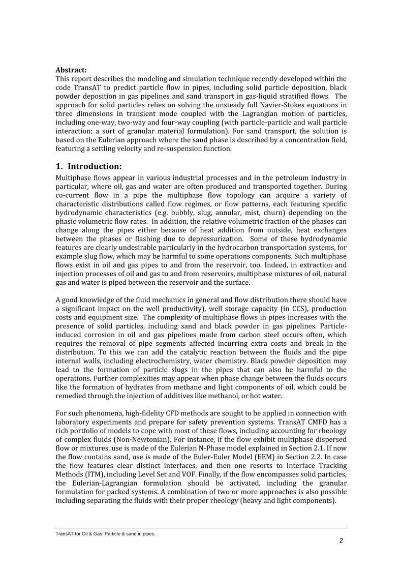
Fig. 1. Settling of a dispersed phase into a Carrier phase by gravity using EEM.

To test the particle settling model (7), we have simulated a generic flow in a square cavity containing water in the form of a dispersed phase, with 1mm droplets mixed within the continuous oil phase. The concentration of water is initially randomly distributed, as shown the first panel of Fig. 1. The settling mechanism is well illustrated in the next panels, with the thickening process of emulsion. The calculation using (6) alone (Stokes velocity) showed a faster settling behaviour than with (7) as is to be expected. In the following part, the model is coupled with the Level Set method to account for the presence of gas, or with Lagrangian particle tracking to account for solid particles.

2.3 Interface Tracking Techniques for Interfacial Flow

Interfacial flows refer to multi-phase flow problems that involve two or more immiscible fluids separated by sharp interfaces which evolve in time. Typically, when the fluid on one side of the interface is a gas that exerts shear (tangential) stress upon the interface, the latter is referred to as a free surface. ITM’s are best suited for these flows, because they


5

represent the interface topology rather accurately. The single-fluid formalism solves a set of conservation equations with variable material properties and surface forces [3]. The strategy is thus more accurate than the phase-average models as it minimizes modeling assumptions. The incompressible multifluid flow equations within the single-fluid formalism read:

Ñ×u= 0 (8)

(9)

where Fg is the gravitational force, Fs is the surface tension force, with n standing for the normal vector to the interface. In the Level Set technique [4] the interface between immiscible fluids is represented by a continuous function , denoting the distance to the interface that is set to zero on the interface, is positive on one side and negative on the other. Material properties, body and surface forces are locally updated as a function of and smoothed across the interface using a smooth Heaviside function:

r, m = r, m

L. H(f) + r, m

G.(1- H(f)) (10)

¶t f + u .Ñf = 0 (11)

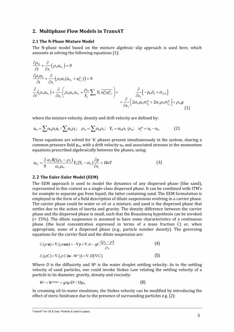
In practice, the level set function ceases to be the signed distance from the interface after a single advection step of Eq. (11). To restore its correct distribution near the interface, a re-distancing equation is advected to steady state, using 3rd - or 5th order WENO schemes; more details can be found in [3]. The method (level set) is used to predict gas-liquid slug flow in pipes (Fig. 2).

Fig. 2. Stratified slug flow in a pipe using ITM (level set technique).

2.4 Lagrangian Particle Tracking

The Eulerian-Lagrangian formulation applies to particle-laden (non-resolved flow or component entities) flows, under one-way, two-way or four-way coupling (also known as dense particle flow system). Individual particles are tracked in a Lagrangian way in contrast to the former two approaches, where the flow is solved in a Eulerian way on a fixed grid. One-way coupling refers to particles cloud not affecting the carrier phase, because the field is dilute, in contrast to the two-way coupling, where the flow and turbulence are affected by the presence of particles. The four-way coupling refers to dense particle systems with mild-to-high volume fractions (> 5%), where the particles interact with each other. In the one- and two-way coupling cases, the carrier phase is solved in an Eulerian way, i.e. mass and momentum equations:

Ñ×u= 0 (12)

(13)


6

combined with the Lagrangian particle equation of motion:

dt (vpi) = - fd

9m

2rpdp2

upi- ui xp(t)éë ùû( ) + g

fd = 1+ 0.15Rep2/3

(14)

where u is the velocity of the carrier phase, up is the velocity of the carrier phase at the particle location, vp is the particle velocity, is the viscous stress and p the pressure. Sources terms in Eq. (13) denote body forces, Fb, and the rate of momentum exchange per volume between the fluid and particle phases, Ffp. The coupling between the fluid and the particles is achieved by projecting the force acting on each particle onto the flow grid:

Ffp =

rpVp

rmVm

Rrc f aW xa ,xm( )a=1

Np

å (15)

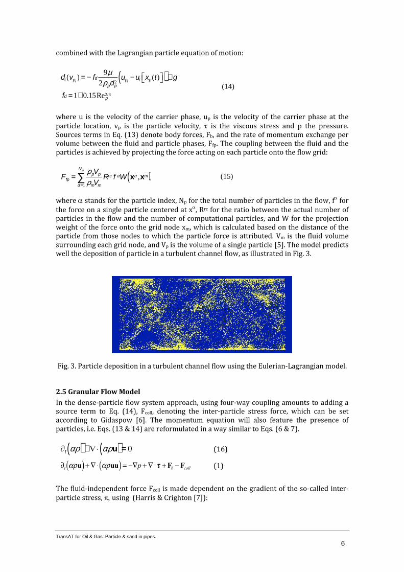
where stands for the particle index, Np for the total number of particles in the flow, f for the force on a single particle centered at x, Rrc for the ratio between the actual number of particles in the flow and the number of computational particles, and W for the projection weight of the force onto the grid node xm, which is calculated based on the distance of the particle from those nodes to which the particle force is attributed. Vm is the fluid volume surrounding each grid node, and Vp is the volume of a single particle [5]. The model predicts well the deposition of particle in a turbulent channel flow, as illustrated in Fig. 3.

Fig. 3. Particle deposition in a turbulent channel flow using the Eulerian-Lagrangian model.

2.5 Granular Flow Model

In the dense-particle flow system approach, using four-way coupling amounts to adding a source term to Eq. (14), Fcoll, denoting the inter-particle stress force, which can be set according to Gidaspow [6]. The momentum equation will also feature the presence of particles, i.e. Eqs. (13 & 14) are reformulated in a way similar to Eqs. (6 & 7).

¶t ar( ) +Ñ× aru( ) = 0

(16)

(1)

The fluid-independent force Fcoll is made dependent on the gradient of the so-called inter-particle stress, using (Harris & Crighton [7]):


7

Fcoll = Ñp / rpa p (2)

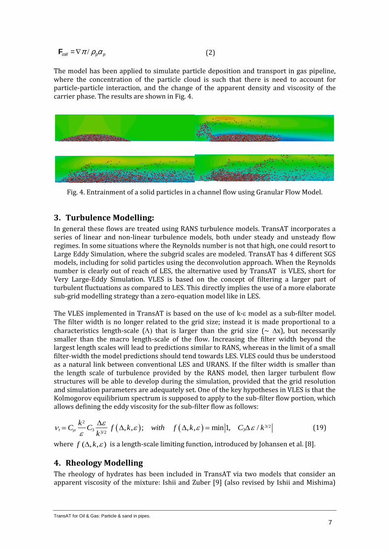
The model has been applied to simulate particle deposition and transport in gas pipeline, where the concentration of the particle cloud is such that there is need to account for particle-particle interaction, and the change of the apparent density and viscosity of the carrier phase. The results are shown in Fig. 4.

Fig. 4. Entrainment of a solid particles in a channel flow using Granular Flow Model.

3. Turbulence Modelling:

In general these flows are treated using RANS turbulence models. TransAT incorporates a series of linear and non-linear turbulence models, both under steady and unsteady flow regimes. In some situations where the Reynolds number is not that high, one could resort to Large Eddy Simulation, where the subgrid scales are modeled. TransAT has 4 different SGS models, including for solid particles using the deconvolution approach. When the Reynolds number is clearly out of reach of LES, the alternative used by TransAT is VLES, short for Very Large-Eddy Simulation. VLES is based on the concept of filtering a larger part of turbulent fluctuations as compared to LES. This directly implies the use of a more elaborate sub-grid modelling strategy than a zero-equation model like in LES. The VLES implemented in TransAT is based on the use of k- model as a sub-filter model. The filter width is no longer related to the grid size; instead it is made proportional to a characteristics length-scale ( that is larger than the grid size (~ x), but necessarily smaller than the macro length-scale of the flow. Increasing the filter width beyond the largest length scales will lead to predictions similar to RANS, whereas in the limit of a small filter-width the model predictions should tend towards LES. VLES could thus be understood as a natural link between conventional LES and URANS. If the filter width is smaller than the length scale of turbulence provided by the RANS model, then larger turbulent flow structures will be able to develop during the simulation, provided that the grid resolution and simulation parameters are adequately set. One of the key hypotheses in VLES is that the Kolmogorov equilibrium spectrum is supposed to apply to the sub-filter flow portion, which allows defining the eddy viscosity for the sub-filter flow as follows:

(19)

where is a length-scale limiting function, introduced by Johansen et al. [8].

4. Rheology Modelling

The rheology of hydrates has been included in TransAT via two models that consider an apparent viscosity of the mixture: Ishii and Zuber [9] (also revised by Ishii and Mishima)

2

3/23 3

3/2, , ; , , min 1, /t

kC C f k with f k C k

k

( , , )f k


8

and Colombel et al. [10] more recent variant. In the first model, which is the mostly used one, the apparent viscosity is defined using this expression:

*2.5

1

pm

pm c

pm

(20)

where pm is the concentration for maximum packing, which for solid particles is equal to 4/7. For solid particles, *= 1, whereas for bubbles and droplets, it takes the form:

0.4*

p c

p c

Colombel et al.’s [10] model, however, accounts in addition for two mechanisms of agglomeration: the first one is the contact-induced agglomeration mechanism, for which the crystallization-agglomeration process is described as the result of the contact between a water droplet and a hydrate particle. The second one is the shear-limited agglomeration mechanism for which the balance between hydrodynamic force and adhesive force is considered. In summary, in this extended model, the viscosity of the suspension is made

proportional to the effective volume fraction eff:

(21)

with μ0 being the oil viscosity and M the maximum packing. The effective volume fraction scales with the actual volume fraction (≈ water cut) as follows:

(22)

5. Selected Results

5.1 RANS vs. LES of Particle Dispersion in a 3D Gas Pipe

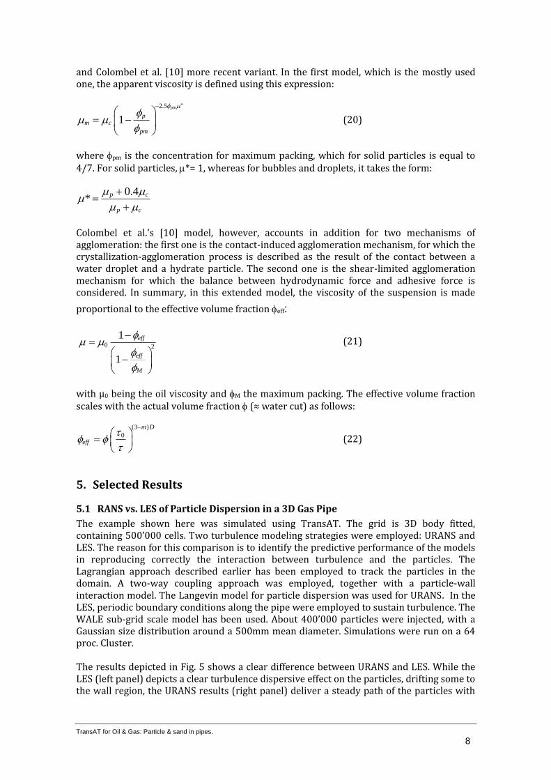
The example shown here was simulated using TransAT. The grid is 3D body fitted, containing 500’000 cells. Two turbulence modeling strategies were employed: URANS and LES. The reason for this comparison is to identify the predictive performance of the models in reproducing correctly the interaction between turbulence and the particles. The Lagrangian approach described earlier has been employed to track the particles in the domain. A two-way coupling approach was employed, together with a particle-wall interaction model. The Langevin model for particle dispersion was used for URANS. In the LES, periodic boundary conditions along the pipe were employed to sustain turbulence. The WALE sub-grid scale model has been used. About 400’000 particles were injected, with a Gaussian size distribution around a 500mm mean diameter. Simulations were run on a 64 proc. Cluster.

The results depicted in Fig. 5 shows a clear difference between URANS and LES. While the LES (left panel) depicts a clear turbulence dispersive effect on the particles, drifting some to the wall region, the URANS results (right panel) deliver a steady path of the particles with

0 2

1

1

eff

eff

M

(3 )

0

m D

eff


9

the mean flow. This is an important result, suggesting that albeit detailed 3D simulations, the results are sensitive to turbulence modeling. Clearly, mechanistic 1D models cannot provide such a picture. Such detailed CFD results could though lend themselves for the development of dispersion models (and also droplet depletion and entrainment models) for the benefit of mechanistic models.

Fig. 5: Snapshots of the flow in a gas pipe showing particle interaction with turbulence: left

(LES); right (RANS).

5.2 Air-Water-Sand in a Pipe

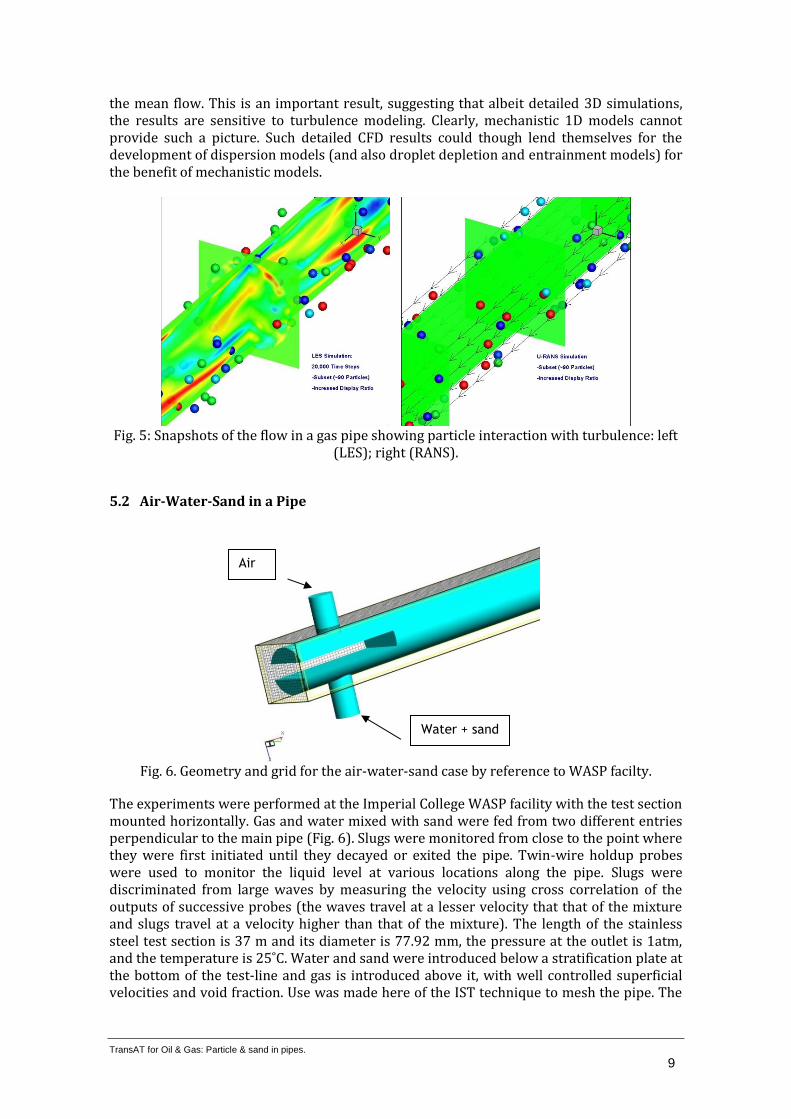
Fig. 6. Geometry and grid for the air-water-sand case by reference to WASP facilty.

The experiments were performed at the Imperial College WASP facility with the test section mounted horizontally. Gas and water mixed with sand were fed from two different entries perpendicular to the main pipe (Fig. 6). Slugs were monitored from close to the point where they were first initiated until they decayed or exited the pipe. Twin-wire holdup probes were used to monitor the liquid level at various locations along the pipe. Slugs were discriminated from large waves by measuring the velocity using cross correlation of the outputs of successive probes (the waves travel at a lesser velocity that that of the mixture and slugs travel at a velocity higher than that of the mixture). The length of the stainless steel test section is 37 m and its diameter is 77.92 mm, the pressure at the outlet is 1atm, and the temperature is 25˚C. Water and sand were introduced below a stratification plate at the bottom of the test-line and gas is introduced above it, with well controlled superficial velocities and void fraction. Use was made here of the IST technique to mesh the pipe. The

Air

Water + sand


10

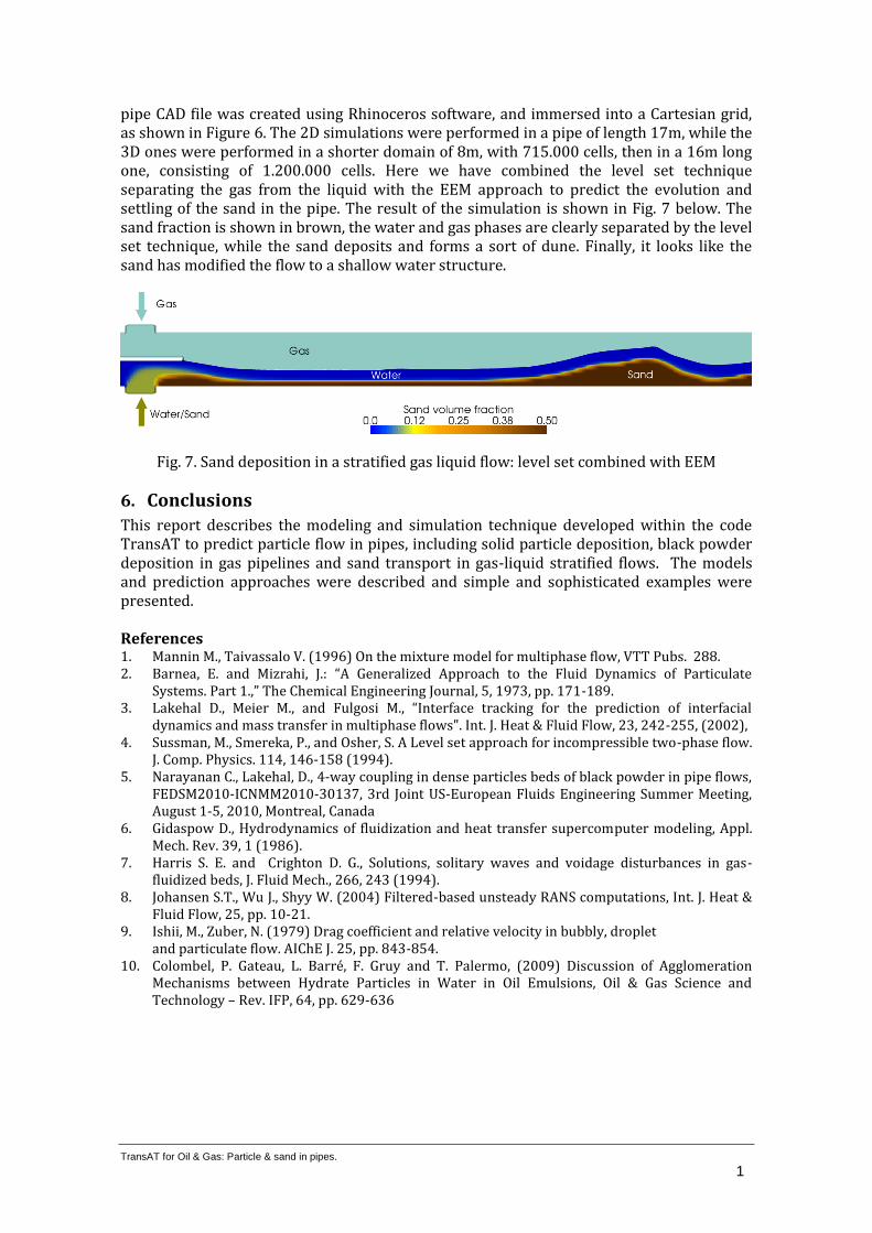
pipe CAD file was created using Rhinoceros software, and immersed into a Cartesian grid, as shown in Figure 6. The 2D simulations were performed in a pipe of length 17m, while the 3D ones were performed in a shorter domain of 8m, with 715.000 cells, then in a 16m long one, consisting of 1.200.000 cells. Here we have combined the level set technique separating the gas from the liquid with the EEM approach to predict the evolution and settling of the sand in the pipe. The result of the simulation is shown in Fig. 7 below. The sand fraction is shown in brown, the water and gas phases are clearly separated by the level set technique, while the sand deposits and forms a sort of dune. Finally, it looks like the sand has modified the flow to a shallow water structure.

Fig. 7. Sand deposition in a stratified gas liquid flow: level set combined with EEM

6. Conclusions

This report describes the modeling and simulation technique developed within the code TransAT to predict particle flow in pipes, including solid particle deposition, black powder deposition in gas pipelines and sand transport in gas-liquid stratified flows. The models and prediction approaches were described and simple and sophisticated examples were presented. References 1. Mannin M., Taivassalo V. (1996) On the mixture model for multiphase flow, VTT Pubs. 288. 2. Barnea, E. and Mizrahi, J.: “A Generalized Approach to the Fluid Dynamics of Particulate

Systems. Part 1.,” The Chemical Engineering Journal, 5, 1973, pp. 171-189. 3. Lakehal D., Meier M., and Fulgosi M., “Interface tracking for the prediction of interfacial

dynamics and mass transfer in multiphase flows". Int. J. Heat & Fluid Flow, 23, 242-255, (2002), 4. Sussman, M., Smereka, P., and Osher, S. A Level set approach for incompressible two-phase flow.

J. Comp. Physics. 114, 146-158 (1994). 5. Narayanan C., Lakehal, D., 4-way coupling in dense particles beds of black powder in pipe flows,

FEDSM2010-ICNMM2010-30137, 3rd Joint US-European Fluids Engineering Summer Meeting, August 1-5, 2010, Montreal, Canada

6. Gidaspow D., Hydrodynamics of fluidization and heat transfer supercomputer modeling, Appl. Mech. Rev. 39, 1 (1986).

7. Harris S. E. and Crighton D. G., Solutions, solitary waves and voidage disturbances in gas-fluidized beds, J. Fluid Mech., 266, 243 (1994).

8. Johansen S.T., Wu J., Shyy W. (2004) Filtered-based unsteady RANS computations, Int. J. Heat & Fluid Flow, 25, pp. 10-21.

9. Ishii, M., Zuber, N. (1979) Drag coefficient and relative velocity in bubbly, droplet and particulate flow. AIChE J. 25, pp. 843-854.

10. Colombel, P. Gateau, L. Barré, F. Gruy and T. Palermo, (2009) Discussion of Agglomeration Mechanisms between Hydrate Particles in Water in Oil Emulsions, Oil & Gas Science and Technology – Rev. IFP, 64, pp. 629-636

Documents

TransAT for Oil & Gas - ASCOMPascomp.ch/.../NOTE-TRANSAT-PARTICLES-in-PIPES.pdf · 2015-08-31 · TransAT for Oil & Gas: Particle & sand in pipes. 2 Abstract: This report describes