Transboundary Pollution in China: A Study of Polluting

HAL Id: halshs-00598592https://halshs.archives-ouvertes.fr/halshs-00598592v2

Preprint submitted on 13 Nov 2012

HAL is a multi-disciplinary open accessarchive for the deposit and dissemination of sci-entific research documents, whether they are pub-lished or not. The documents may come fromteaching and research institutions in France orabroad, or from public or private research centers.

L’archive ouverte pluridisciplinaire HAL, estdestinée au dépôt et à la diffusion de documentsscientifiques de niveau recherche, publiés ou non,émanant des établissements d’enseignement et derecherche français ou étrangers, des laboratoirespublics ou privés.

Transboundary Pollution in China: A Study of PollutingFirms’ Location Choices in Hebei Province

Chloé Duvivier, Hang Xiong

To cite this version:Chloé Duvivier, Hang Xiong. Transboundary Pollution in China: A Study of Polluting Firms’ LocationChoices in Hebei Province. 2012. �halshs-00598592v2�

https://halshs.archives-ouvertes.fr/halshs-00598592v2

https://hal.archives-ouvertes.fr

CERDI, Etudes et Documents, E 2011.17

Document de travail de la serie

Etudes et Documents

E 2011.17

Transboundary Pollution in China: A Study of Polluting

Firms’ Location Choices in Hebei Province

Chloe Duvivier and Hang Xiong

May, 2011

(revised September 2012)

CERDI

65 BD. F. MITTERRAND

63000 CLERMONT FERRAND - FRANCE

TEL. 04 73 71 74 20

FAX 04 73 17 74 28

www.cerdi.org

1

www.cerdi.org


Les auteurs

Chloe Duvivier (corresponding author)

Doctorant / PhD Student

Clermont Universite, Universite d’Auvergne, CNRS, UMR 6587, CERDI, F-63009

Clermont Fd.

Email : [email protected]

Hang Xiong

Doctorant / PhD Student

Clermont Universite, Universite d’Auvergne, CNRS, UMR 6587, CERDI, F-63009

Clermont Fd.

La serie des Etudes et Documents du CERDI est consultable sur le site :

http://www.cerdi.org/ed

Directeur de la publication : Patrick Plane

Directeur de la redaction : Catherine Araujo Bonjean

Responsable d’edition : Annie Cohade

ISSN : 2114 7957

Avertissement :

Les commentaires et analyses developpes n’engagent que leurs auteurs qui restent

seuls responsables des erreurs et insuffisances.

2

http://www.cerdi.org/ed


Resume / abstract

Transboundary pollution is a particularly serious problem as it leads people lo-

cated at regional borders to disproportionately suffer from pollution. In China,

where the environmental policy is decentralized and where environmental con-

flicts between provinces have occurred several times, transboundary pollution is

likely to exist. However, until now, nearly all the studies focused on developed

countries. In this paper, we study whether transboundary pollution problems

exist in China. To do so, we estimate whether, within Hebei province, polluting

firms are more likely to set up in border counties than in interior ones. To en-

sure the robustness of our results, several measures of the variable of interest are

constructed from Geographic Information System (GIS) data. The estimations

of a count-data model allow us to conclude that border counties are more attrac-

tive destinations for polluting firms than counties located within the province.

Moreover, it appears that this effect has strengthened over time.

Mots cles /Key words : Transboundary pollution, firm location choice, environ-

mental regulations, China

Codes JEL / JEL codes : Q01, Q56

Remerciements

We are thankful to E. Langlois and O. Santoni for their help with GIS data. We

are also grateful to J-L. Combes, C. Ebeke, S. Poncet and participants at Peking

University seminar, at PACE 2011 International Symposium on Environmental

Economics and Policy in China (Hangzhou, July 2011) and at the Conference

for Sustainable Attractivity (Bordeaux, September 2011) for constructive sugges-

tions.

3


1. Introduction

In recent years, more and more environmental conflicts between provinces have been

attracting great attention in China. For example, in January 2008, residents of the

Wuqing district (Tianjin province) complained that a cement plant in the neighboring

Xianghe county (Hebei province) had over-discharged dust pollution which then crossed

the province border and damaged their soil and crop production (Wuqing District En-

vironmental Protection Bureau, 2008). Disputes involving the Huai River, which runs

through Henan, Shandong, Anhui and Jiangsu provinces, are also very illustrative of ever-

increasing transborder conflicts. On several occasions, downstream provinces have accused

upstream provinces of dumping pollution into the river in order to evacuate it to other

provinces. As polluters from a given province can evacuate a part of their pollution to

other provinces, there is a risk of excess of pollution at regional borders of the countries.

There is already quite strong evidence that a decentralized environmental policy can

lead to pollution havens and free-riding effects, resulting in an excess of pollution at

regional borders. This is what is known as transboundary pollution. Transboundary

pollution is a very serious problem as it appears that people in border counties suffer

disproportionate health problems as a result of pollution. Indeed, in the United States,

cancer rates are substantially higher in border counties than in interior ones due to trans-

boundary pollution (Kahn, 2004). Until now, almost all studies have been focused on

the United States (Helland and Whitford, 2003; Kahn, 2004; Sigman, 2005; Konisky and

Woods, 2010). Very few have looked at this issue in emerging countries. Lipscomb and

Mobarak (2011) constitute one exception, with their analysis of water pollution spillovers

in Brazil.

China meets all the conditions that make it susceptible to the emergence of trans-

boundary pollution. Indeed, China’s environmental policy is decentralized: while the

central government sets environmental standards, it is the local governments who monitor

and impose sanctions on polluters. In the Chinese context, as we will see in more details in

Section 3, there is a high probability for the existence of free-riding and pollution havens.

In addition, environmental conflicts between provinces provide some evidence that trans-

4


boundary pollution is already occurring. However, until now, transboundary pollution in

China has not received the attention it deserves, primarily due to the lack of available

data.

This study contributes to the literature by studying whether or not transboundary

pollution does indeed exist in China today. To address this question, we study the lo-

cation choice of polluting firms between 2002 and 2008 in Hebei, one of the most highly

polluted provinces in the country. Specifically, we test whether polluting firms are more

likely to set up in counties1 that share a border with another province than in interior

counties. For this purpose, we use the lists of polluting firms published annually by the

Ministry of Environmental Protection and by the Environmental Protection Bureau of

Hebei Province. To ensure the robustness of our results, several measures of the variable

of interest have been constructed from Geographic Information System (GIS) data. We

find very robust evidence even after controlling for confounding factors such as market ac-

cess, that border counties are more attractive destinations for polluting firms than interior

counties. Moreover, it appears that this effect has been increasing over time.

By demonstrating that border county residents are more highly exposed to pollution,

we also contribute to the very scarce literature on environmental inequality in China.

Two notable exceptions are Ma (2010) and Schoolman and Ma (2011), who investigate

how socioeconomic characteristics of townships influence the geographic repartition of

pollution. Ma (2010) highlights that rural residents, and especially rural migrants, suffer

disproportionately from pollution in Henan. Schoolman and Ma (2011) emphasize that

migrants are disproportionately exposed to pollution in Jiangsu and put forth a general

theory of environmental inequality by highlighting that in China, as in the US, individuals

at the bottom of the social ladder bear most of the environmental burden. By proposing

an additional lens (proximity to regional borders) to analyze environmental inequality,

the present study provides complementary results to these previous works.

1The ”county” corresponds to the third level of administrative division in China. There are three types

of administrative divisions at the county level in China: prefectural city districts (shıxiaqu), cities at the

county level (xianjishı) and counties (xian).

5


The remainder of the article is organized as follows. Following the introduction, in

Part Two we briefly present China’s environmental policy. Next, we study why, in the

context of a decentralized policy, polluting firms would tend to agglomerate near regional

borders. Part Four describes the study area and the data. We present the estimation

strategy in Part Five and the results in Part Six. Finally, we conclude and offer some

policy recommendations.

2. Environmental policy in China

2.1. A decentralized environmental policy

During the 1980s, China’s environmental policy followed the general trend of decen-

tralization occurring in the country and since then, its enforcement has depended largely

on local governments. Environmental protection is currently managed at the national level

by the Ministry of Environmental Protection (MEP) and, at the regional and local levels

(provinces, prefectures and counties), by the Environmental Protection Bureaus (EPBs).

The central government establishes environmental standards and environmental policy is

implemented by the regions which monitor emissions and impose penalties if standards

are not met. Decentralization of environmental policy in a country as heterogeneous as

China offers undeniable advantages. Indeed, it allows for greater flexibility as well as

better information and adaptation to the local context. However, as local officials are

evaluated more on economic than on environmental performance, environment protection

is often sacrificed for economic gain, resulting in significant environmental degradations.

Facing this critical situation, a certain ”recentralization” of China’s environmental pol-

icy has occurred. In 2008, the State Environmental Protection Agency (SEPA) became

the MEP in order to give more power back to the central government. Moreover, be-

tween 2006 and 2008, six major supervision centers were created. Each of these major

centers is responsible for several provinces and monitors whether or not they respect the

environmental standards established by the central government. These centers are also in

charge of coordinating interprovincial conflicts. Thus, they constitute a new intermediary

level between central government and provinces, established with the aim of limiting the

negative effects of decentralization. However, until now, the power of these new centers

6


has been very limited and environmental policy is still largely implemented by Chinese

provinces.

2.2. Impact of environmental regulations on polluting firms

Like all firms, those that pollute do not choose their location randomly: they decide

to locate in a particular region to maximize their profit. Several studies show that in

China, the location choice of both foreign (Wu, 1999) and Chinese firms (Wen, 2004)

depends today on ”rational economic considerations”. Thus, firms are generally attracted

to regions with good market opportunities and where labor is cheap and skilled.

Polluting firms, in addition, usually take into account the severity of environmental

regulation when deciding where to set up. This is likely to be the case in China, where

it has been shown that environmental regulations significantly raise the costs of polluting

firms. For example, Wang (2002) estimates that pollution charges lead to a significant

increase in expenditures on end-of-pipe water treatment facilities at the plant-level. More-

over, a higher number of inspections leads to a higher expected penalty for firms that do

not comply with environmental standards and thus, significantly reduces the level of water

and air pollution of industries in the city of Zhenjiang (Dasgupta et al., 2001). In addi-

tion, although state-owned enterprises have more bargaining power with local authorities

in terms of the charges they pay (Wang et al., 2003), environmental policy also has a

significant impact on them (Wang and Wheeler, 2005). As a consequence, given that

environmental regulation in China imposes significant costs on polluting firms, we would

expect these firms to locate in regions with less stringent environmental regulation.

3. Literature review: why would polluting firms be more likely to set up near

borders?

As explained in Section 2.2., polluting firms are expected to set up in regions with less

stringent environmental regulations. In this section, we explain how regional differences

in environmental regulations lead polluting firms to set up more frequently in border

counties. Specifically, two phenomena could lead to transboundary pollution, namely

”pollution havens” and ”free-riding” effects.

7


3.1. Differences in interprovincial regulation: pollution havens hypothesis at the provincial

level

In China, environmental policy implementation varies greatly from one province to

another (Wang and Wheeler, 2005). Such disparity in policy enforcement by region would

be at the origin of a ”pollution havens”phenomenon at the provincial level2: polluting firms

would be attracted to provinces where environmental regulations are less strict (Dean et

al., 2009). Indeed, at the borders, there are discontinuities in environmental regulations

(Kahn, 2004). By crossing an administrative boundary, one can suddenly move from

strict environmental regulation to a less restrictive one. In this context, it could be very

profitable for a firm to locate on the border between two provinces. Crossing a border

can therefore be a way to avoid stringent environmental regulations while continuing to

benefit from the market access of the neighboring province with stricter environmental

regulation. Kahn (2004) shows that in the United States, in low environmental regulation

states, ”dirty” industries set up more often in counties that border high regulation states

than in interior counties. Conversely, in counties bordering low regulation states, there

is a lower number of polluting firms. In terms of environmental regulation, Hebei is

less stringent than its neighbors, with the exception of Inner Mongolia3. Thus, on the

whole, we can expect the pollution havens effect to be positive in Hebei province, leading

polluting firms to concentrate close to borders.

2The hypothesis of ”pollution havens” is generally considered at the international level. According to

this hypothesis, in a world of free trade, the South, whose environmental regulations are less stringent,

has a comparative advantage in producing ”dirty” goods. This can lead polluting industries to migrate

from the North to the South.3Using data from the 2002 China Environment Yearbook, we calculate two indicators at the provincial

level to measure environmental stringency: the levy fees divided by the number of charged organizations

and the share of industrial pollution treatment investment in innovation investment. In each case, Inner

Mongolia is the only neighboring province with less stringent regulation than Hebei (results available

on request). Dean et al. (2009) obtain the same ranking using the average collected levy per ton of

wastewater as the indicator of de facto provincial stringency.

8


3.2. Differences in intra-provincial regulations: free-riding and intra-provincial pollution

havens hypotheses

When environmental policy is decentralized, provincial regulators may be less strict

in implementing the policy in border counties than in interior ones. In other words, free-

riding may emerge at the boundaries between different regions of the country4. Two fac-

tors could encourage regulators to strategically implement environmental regulation, both

leading to an excess of pollution at borders. First of all, at borders, a region’s expenditure

on pollution control does not solely benefit that region; it also benefits neighboring ones

(Sigman, 2002). Since regions have limited financial resources, they prefer investing funds

where they can reap the highest benefit, that is to say, in interior counties. Secondly, at

borders, some of a given firm’s pollution impacts the neighboring region. Thus, in border

counties, the population benefits from the overall positive economic advantages related to

the presence of the firm (jobs and taxes) and only suffers from part of the pollution gener-

ated (Helland and Whitford, 2003). On the contrary, in interior counties, the population

benefits from job opportunities but must also bear all the pollution generated. Thus, we

would expect social discontent related to the establishment of a polluting firm to be higher

in interior counties. As a result, a regulator concerned with political support5 and job

promotion6 will be more likely to oppose the arrival of a polluting firm and to apply more

stringent environmental regulations in interior counties. The same free-riding argument

applies to coastal counties, explaining why emissions are much higher in these counties

(Helland and Whitford, 2003). It is worth noting that the free-riding effect will always

4”Region” here refers to a U.S. state or a Chinese province.5The Chinese authorities have to address a large and growing number of citizen complaints about

pollution. There were already 138495 letters of complaint in 1993 (Dasgupta and Wheeler, 1997). In

2002, 428626 letters were sent to the authorities (State Environmental Protection Agency, 2003). In some

extreme cases, local officials lost their posts because of public pressure after environmental crises. For

example, in 2009, in the wake of a great amount of intense public pressure, numerous local officials were

dismissed because of pollution accidents in Hunan, Shaanxi and Inner Mongolia.6The political promotion system in China has evolved over time. While promotion used to be based

solely on economic performance, since 2005 experiments have been conducted in some provinces where

promotion depends now both on economic and environmental performance.

9


lead polluting firms to concentrate in border counties, whatever the relative stringency of

Hebei’s environmental regulation. However, the magnitude of the effect is reduced when

the neighboring state enforces stringent environmental regulation (Gray and Shadbegian,

2004).

Finally, the strategic implementation of environmental regulation (less stringent regu-

lation at borders) can also lead to an intra-provincial pollution havens effect. Because of

their less stringent regulation, we would expect border counties to attract more polluting

firms than interior borders, leading to transboundary pollution.

4. Description of the study area and data

4.1. Hebei province

This study is carried out in Hebei Province for several reasons. First of all, Hebei has

been industrialized for many decades, which makes it one of the most polluted provinces

in the country. According to the list published in 2010 by the Chinese government, which

identifies the most polluting firms in China, 744 of the 9833 top polluters in China are

located in Hebei. The province has the highest number of polluting firms just after Jiangsu

(838) and Shandong (774). Moreover, Hebei shares borders with seven other provinces

including the provincial cities of Beijing and Tianjin (see Figure 1). In addition, Hebei

has already been involved in several transboundary pollution conflicts, as stated in the

introduction. Finally, Hebei is one of the few provinces with the necessary data available

to allow us to carry out our study.

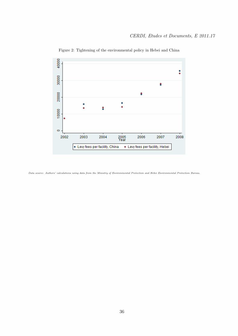
Regarding environmental protection, environmental policy in Hebei province has been

continuously tightened since the beginning of the 2000s as shown in Figure 2. Thus, we

can expect polluting firms to be increasingly sensitive to environmental regulation over

the period under study. As discussed in Section 6.4, this may have led polluting firms to

increasingly settle close to borders over the past few years.

[Figure 1 here]

[Figure 2 here]

10


4.2. Construction of the dependent variable and sample

The dependent variable of our model is the annual number of polluting firms set up by

county. We constructed this variable from the lists published by the MEP and the EPB of

Hebei7. Since 2007, the MEP and EPBs of provinces annually publish lists (Guojia/Sheng

zhongdian jiankong qiye mingdan) that identify the most polluting firms in China8. These

lists give the name of each firm and the county in which it is located. Moreover, the lists

classify each firm as: ”water polluting firm”, ”air polluting firm”or ”waste water treatment

facility”. Waste water treatment facilities are always built close to population centers in

order to treat municipal waste. As they do not freely choose their location, transboundary

pollution is not likely to occur in this case, and therefore, we have excluded them from our

analysis. By contrast, both air and water pollutant firms freely choose their location and

thus, take into account environmental regulation when deciding where to set up. Thus,

we consider both air and water polluting firms when constructing our dependent variable.

However, the MEP and EPBs lists provide no information regarding a firm’s estab-

lishment date or emissions level. So, these lists give the necessary information to estimate

a model of stock, in which the total number of firms in a county is regressed on a set of

regional variables. However, in this study we estimate a flow model in which the number

of firms created in a county at year t is regressed on the characteristics of this county at

year t. Indeed, as there was no environmental policy in China before 1979, to test the

existence of transboundary pollution, we were obliged to take a sample of firms which

have been recently created and which are, therefore, sensitive to environmental regula-

tion. In addition, the flow model enables us to test whether transboundary pollution has

increased over time. In order to estimate a flow model, we have collected the creation

dates of polluting firms from the official website of the Industrial and Commercial Bureau

7To our knowledge, Ma (2010) is the first to use this data list for Henan province.8The lists identify the most polluting firms at national and provincial level in terms of air, water and

sewage pollution. More precisely, the firms identified produce 65% of total industrial emissions of SO2,

NOx, COD, NH3-N and heavy metals. As these pollutants can cross regional borders, this data enables

us to test for transboundary pollution. Note that there is a lag of two years between the census of firms

in the list and their pollution. Thus, the 2007 list contains the firms that polluted the most in 2005.

11


of Hebei province.

Once the creation dates were obtained, we selected firms set up after 2002, year from

which we have data for the explanatory variables. In addition, the last list of polluting

firms was published in 2010; it lists the most polluting firms in 2008. Thus, our sample

covers the period of 2002-2008. In all, 253 air and water polluting firms were set up in

Hebei province between 2002 and 2008.

4.3. Variables of interest

Three variables of interest have been constructed to ensure robustness. Firstly, we

follow the literature (Helland and Whitford, 2003; Kahn, 2004; Konisky and Woods, 2010)

and construct a dummy variable equal to 1 if the county shares a border with another

province, or the sea, and 0 otherwise (Border 1). As explained in Section 3.2, the same

free-riding phenomenon is expected to take place in coastal counties. Thus, to capture

the whole transboundary pollution effect, we first create a variable including both coastal

and other border counties. However, as can be seen in Figure 1, some border counties

share a very small part of their border with another province while others share more

than half of the total length of their border with another province. To take into account

the variability among border counties, we create a second variable equal to the length

of the common border with another province (or the sea) divided by the total length of

the county’s border (Border 2). The drawback of the first two variables is that they do

not take into account the variability between non-border counties: while some counties

are located at the center of the province, others are very close to the borders. Moreover,

both measures are likely to be significantly affected by the shape of the county. For these

reasons, we create a third variable equal to the distance between the county seat and

the closest border (Distance)9. These variables have been constructed with GIS data,

using ArcGis 9.2. If transboundary pollution exists, we expect polluting firms to be more

likely to set up near borders. Therefore, we would expect the coefficients associated with

9Following Gray and Shadbegian (2004), we created a dummy equal to one if the county seat is located

within 50 miles of the border to another province as a fourth indicator of Border. Results, available upon

request, are robust to this alternative measure.

12


variables ”Border 1” and ”Border 2” to be positive and the coefficient associated with

”Distance” to be negative.

Table 1 gives descriptive statistics on the polluting firms in our sample. Panel A of

the table gives the average stock of firms in 2001 and 2008 for all counties, border and

non-border. Interestingly, non-border counties had a slightly higher number of polluting

firms than border counties in 2001 whereas the opposite was true for 2008.

[Table 1 here]

Panel B of the table gives data on firm births from 2002 to 2008. It clearly indicates

that over the recent period, polluting firms have located significantly more frequently in

border counties, which tends to validate the transboundary pollution hypothesis. More-

over, the differences observed in the stock of firms between non-border and border counties

reflect an evolution in polluting firms’ location choices in China. Among the firms iden-

tified in the lists, some were created before the 1980s. At that time, a firm’s location

decision was not based on economic rationale but rather arose from a strategy aimed at

protecting industries from potential destructive military conflicts. From 1965 to 1978,

three principles determined the location choice of industrial firms: ”proximity to moun-

tains, dispersion and concealment” (Wen, 2004). Thus, industrial firms were located far

away from the coast. Moreover, an environmental policy did not yet exist in China.

Therefore, it should not be a surprise that the stock of firms in 2001 was not higher in

border counties than in non-border counties. By contrast, newly created polluting firms

choose their location according to economic criteria and certainly take into account the

degree of environmental policy implementation. As a result, transboundary pollution is

likely to exist and this would explain why, nowadays, polluting firms would set up more

in border counties than previously.

Figure 1, which shows the positions10 of the polluting firms created between 2002 and

2008, also gives interesting insights about transboundary pollution. Indeed, firms seem

10The lists published by the MEP and the EPB do not report the geographical coordinates of polluting

firms. Following Ma (2010) and Schoolman and Ma (2011), we have collected the geographical coordinates

of polluting firms.

13


to locate more often in counties close to Tianjin, Shanxi, Henan, and to some extent, to

Shandong. This transboundary pollution effect is reinforced by the fact that many firms

set up in the capital Shijiazhuang, which is close to the regional border. Surprisingly,

despite its high market potential, Beijing does not appear to significantly attract polluting

firms. This could be due to the fact that free-riding is reduced when the neighboring state

possesses stringent environmental regulation (Gray and Shadbegian, 2004). Interestingly,

there are very few firm births close to Inner Mongolia. As explained in Section 3.1, Inner

Mongolia has less stringent environmental regulation than Hebei which, according to the

pollution haven hypothesis, would be expected to lead to fewer firm births in counties

bordering Inner Mongolia.

4.4. Other determinants in a polluting firm’s location choice

As control variables, we introduce the traditional determinants of a firm’s location,

i.e. the regional characteristics that may affect the firm’s profit. Firstly, a number of

variables affect a firm’s revenue. On the one hand, firms are attracted to regions with

agglomeration economies (Arauzo-Carod et al., 2010) i.e., to counties where there is a

strong spatial concentration of economic activity. This enables firms to benefit from

good access to intermediate inputs, from market opportunities and from information. On

the other hand, firms are more likely to set up in regions that offer significant market

opportunities. Generally, firms do not consider only the local market but also the markets

of neighboring regions, or ”external market” (Head and Mayer, 2004). The local market

is measured by the county’s population. Following Holl (2004), the external market is a

spatial lag variable of the following form:

External marketit =∑

j

wij · Popjt

where i refers to the county (county, districts or city at county level) and j the city

(prefectural-level or county-level city). Popjt refers to the population11 of city j at year

t. The contiguity matrix wij is equal to 0 if i and j do not share any border and to

11We use the population of the city to represent the size of the market in neighboring cities because

population has been shown to be a good proxy of demand access (Holl, 2004).

14


the inverse of the number of kilometers from the county seat of i to the county seat of

j if i and j share a common border. Furthermore, as regions whose population is well

educated are likely to attract firms, we introduce an indicator of the level of education of

the county population. We also control for the presence of national and provincial-level

Special Economic Zones (SEZ) as regions benefiting from SEZ status attract significantly

more firms (Wu, 1999). We also introduce a dummy indicating whether the county has

an international port, to control, to some extent, for international market access. Finally,

recent studies have demonstrated that there is an inverted U-shaped relationship between

environmental degradation and income per capita in China (Song et al.,2008; Jalil and

Mahmud, 2009). To test for the existence of a Kuznet relationship, we include the GDP per

capita and its square12. As we expect the relationship between environmental degradation

(proxied by the number of polluting firm births) and income per capita to be initially

positive and then to turn negative once a certain threshold is reached, we would expect

the coefficient associated to GDP per capita and to its square to be respectively positive

and negative.

Furthermore, as firms are attracted by regions where production factors are cheap, we

introduce the real wage rate in industry as a proxy for labor price.

Finally, we introduce a set of indicators for natural endowments. First, we introduce

the land area of the county, which is expected to positively affect the number of firm

births, as it is a proxy for the number of potential sites (Bartik, 1985). Second, the length

of rivers running through each county is also introduced, given that many plants need to

be located close to freshwater (Ma, 2010). Third, as it may be more difficult for a firm

to set up in a mountainous area, we control for the topography of the county. Note that

the last two control variables are particularly important given that borders are sometimes

established by geographical discontinuities (rivers or mountains), which could bias our

estimation of the transboundary effect (Holmes, 1998). Lastly, we introduce a dummy

variable for districts to reflect the nature of the administrative unit and year dummies in

12GDP per capita also controls for the level of development of the county and thus, for some variables

for which we do not have any information (for example, infrastructures).

15


every specification. All of this data comes from the Hebei Statistical Yearbooks (2003-

2009); the definition of variables and descriptive statistics are provided in Appendix A13.

5. Estimation strategy

The dependent variable of the model is the number of polluting firms created in county

i at year t. The special nature of the dependent variable (non-negative integers with a

high frequency of zeros) has led us to estimate a count-data model. This model estimates

how much a 1% change in an explanatory variable xi affects the probability that a firm

sets up in territory i. The probability, Prob(yi), of a territory i to receive yi firms is based

on a set of characteristics xi of this territory:

Prob(yi) = f(xi)

The most common way to model this probability function is to assume that the variable

yi follows a Poisson distribution. However, the Poisson model is restrictive because it

assumes that the conditional mean is equal to the conditional variance of yi (hypothesis

of equi-dispersion). The hypothesis of equi-dispersion is poorly respected with data on

firms’ location choices, as the conditional variance is often higher than the conditional

mean, referred to as ”overdispersion”. Two phenomena can lead to overdispersion: (i) the

presence of unobserved heterogeneity and (ii) an excess of zeros.

13The province of Hebei contains 172 county level divisions: 36 districts, 22 county-level cities and 114

counties. For the districts of the 11 prefecture cities where disaggregated data is not available, the districts

of a prefecture city are aggregated. Therefore, our sample is constituted of 147 units at the county level.

If a prefecture city is composed both of border and interior districts, such aggregation would lead us to

consider all of the districts as one unique border district, artificially increasing the number of firms births

in border districts. This could lead to an upward bias of the results. However, among the 11 prefecture

cities, Tangshan is the only one to be composed both of border and interior districts. The remaining

ten cities are composed either only of border districts or of interior districts, ruling out any potential

bias. In order to check whether the aggregation of the districts in Tangshan leads to bias estimates,

we run additional estimations by dropping the polluting firms which set up in the interior districts of

Tangshan. Results, which are available upon request, clearly show that the aggregation does not induce

bias estimates.

16


When overdispersion arises from unobserved heterogeneity, standard deviations ob-

tained are biased and therefore, statistical inferences are invalid. In this case, the standard

solution consists in assuming that the variable yi follows a negative binomial distribution.

It can be easily determined whether the negative binomial model is preferred to the Pois-

son model, by testing whether the parameter alpha is statistically different from zero (see

Cameron and Trivedi, 1998).

When overdispersion arises from an excess of zeros (or ”zero inflation”), the dependent

variable yi takes the value zero more times than assumed by the Poisson distribution,

which results in biased estimates. Zero inflation arises when two separate processes lead

the dependent variable to take the value zero. In the present study, two processes are

likely to explain why some counties did not attract any polluting firms from 2002 to 2008.

On the one hand, some counties may not be suitable locations for firms and thus, they

will never attract any, whatever the period considered. This could be the case for counties

lacking a river, in mountainous areas and where there are no market opportunities. On

the other hand, some counties may be suitable locations for firms but did not attract

any new firms from 2002 to 2008. To distinguish between the two processes generating

a zero outcome, Greene (1994) proposes estimating a zero-inflated Poisson (ZIP) model

which essentially consists in integrating a probit model into the Poisson regression model.

Specifically, a probit equation is first estimated to distinguish those territories that will

never attract any firms from the others. In a second-step, the standard Poisson model is

estimated.

Lastly, overdispersion can arise both from unobserved heterogeneity and from an excess

of zeros. The suitable model in this case is the zero-inflated negative binomial (ZINB)

model.

Table 2 gives some insight about the potential zero inflation problem in our sample.

The table represents the frequency and percentage of counties with 0, 1, 2, ... , creations

of firms from 2002 to 2008. According to panel B of the table, when considering the panel

dimension of our data, the dependent variable takes the value zero in as much as 84.74%

of the cases. The frequency of zeros in our sample is comparable to those in List (2001)

and Roberto (2004) who estimate a zero-inflated model.

17


[Table 2 here]

In terms of the testing procedure, as the Poisson (negative binomial) model and the

ZIP (ZINB) model are not nested, the Vuong test (1989) is used to test for zero-inflation.

Asymptotically, the Vuong test statistic has a standard normal distribution and hence, the

test statistic obtained must be compared with the critical value of the normal distribution

(1.96). A value above 1.96 (below -1.96, respectively) rejects the standard model (zero-

inflated model) in favor of the zero-inflated model (standard model).

6. Estimation results

6.1. Testing for the appropriate model

To determine the model that best fits our data, we (i) test the validity of the equi-

dispersion hypothesis and (ii) investigate the source(s) of overdispersion.

Appendix A already gives us some insight about the presence of overdispersion in our

data. Indeed, the standard deviation of the dependent variable is more than three times

its mean. In addition, we estimate the model assuming that the number of firm births

follows a Poisson distribution14. The chi-square value obtained is very high, indicating

that the Poisson distribution is not suitable (see Cameron and Trivedi (1998)).

The second step consists in testing whether overdispersion arises from unobserved

heterogeneity and/or from an excess of zeros. As shown in Table 2, we are very likely to

face a problem of zero-inflation, which could lead to biased estimates. Thus, we further

investigate the presence of zero inflation with the Vuong test. The Vuong statistics are

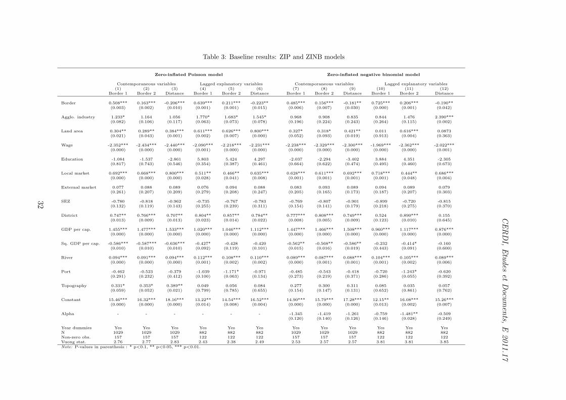
reported at the bottom of Table 3. Table 3 gives the estimation results of the ZIP and

of the ZINB models15. In each case, six different equations are estimated, depending on

14Results available upon request.15For convergence issues, and following Roberto (2004) and Konisky and Woods (2011), we introduce a

subset of the explanatory variables in the first-stage model. Specifically, to differentiate between counties

that are unsuitable for firm’ locations and counties suitable for firms’ location, we introduce the following

variables in the probit model: agglomeration in industry, education, market, topography, river and a time

trend. We carry out estimations with different subsets of variables and obtain similar results. Results of

the first-step model are available in Appendix B.

18


the variable of interest introduced (Border1, Border2 and Distance) and on whether

or not a time lag is introduced between the dependent and the explanatory variables16.

In all twelve cases, the Vuong test clearly rejects the standard model in favor of the

zero-inflated model, indicating that zero inflation must be taken into account to obtain

consistent estimates.

In addition, the parameter alpha estimated with the ZINB model provides information

on whether overdispersion also arises from unobserved heterogeneity. In 5 cases out of 6,

the parameter is not statistically different from zero, indicating that the ZIP better fits

our data17. As a consequence, in this paper, we carry out the analysis by estimating a

pooled ZIP model, which enables us to take into account overdispersion arising from an

excess of zeros.

[Table 3 here]

6.2. Does transboundary pollution exist in China?

According to Table 3, the variable of interest has the expected sign and is statistically

significant in every case. Counties that share a (larger part of their) border with another

province or with the sea have a higher probability of polluting firms locating there. In the

same way, the further the county seat is from the boundary, the lower the probability of

polluting firms settling there. These results provide evidence of transboundary pollution

problems in China. If this has already been demonstrated for the U.S. case, to our

knowledge, we are the first to demonstrate this phenomenon in China.

Regarding the control variables, their sign and significance are consistent and robust.

The larger the land area, the local market and the GDP per capita, the higher the number

16Firstly, we regress the number of firms created at year t on the values of the explanatory variables in

t. Secondly, we use lagged explanatory variables by regressing the number of firms created at year t on

the values of the explanatory variables in t − 1. Using lagged explanatory variables enables us both to

rule out endogeneity and to take into account the time dimension of the decision process (firms often set

up at year t after having observed the county’s characteristics in the previous year).17Moreover, we run estimations of the ZINB model for all specifications of the paper. In every case,

the results obtained are very similar to those obtained with the ZIP model, indicating that there is no

need to take into account unobserved heterogeneity.

19


of firm births. Conversely, the higher the labor costs, the lower the number of firm births.

Moreover, polluting firms set up more frequently in urban districts and in counties where

fresh water is available. This confirms that the location choice of Chinese firms nowadays

is based on economic factors.

6.3. Robustness checks

According to the above estimates, we conclude that there is transboundary pollution

in Hebei. However, polluting firms could set up in border counties for other factors, and

in particular to benefit from better market access. Indeed, Hebei is a very unique province

in terms of its geography as it (i) shares borders with the Yellow Sea and (ii) surrounds

Beijing and Tianjin municipalities (see Figure 1). Thus, polluting firms could set up more

frequently in border counties in order to benefit from the access to international markets

or from the proximity to Beijing and Tianjin markets. The two following subsections

further test for transboundary pollution by explicitly controlling for international market

access and for the proximity to Beijing and Tianjin.

6.3.1. Transboundary pollution or access to international markets?

To check whether our results are driven by international market access, we separate

counties that share a common border with another province from those that share a border

with the sea18. ”Terrestrial border” refers to counties that border another province while

”maritime border” refers to counties bordering the Yellow Sea19. If polluting firms set up

in border counties only to benefit from good access to international markets, the coefficient

associated with the variable terrestrial border should not be significant. The results of the

estimations, given in panel A of Table 420, clearly indicate that the results are not driven

by international market access. Indeed, in every estimation, the coefficient associated with

the variable terrestrial border is of expected sign and statistically significant.

18It is also interesting to distinguish coasts from other borders because when polluting firms locate in

coastal counties, they do not impose any costs on their neighbors, resulting in lower social welfare losses.19For the third indicator of interest (Distance), ”terrestrial border” (”maritime border”) refers to the

shortest distance between the county seat and any provincial border (the sea).20Table 4 only presents the coefficients of interest. The full estimation results are available upon request.

20


[Table 4 here]

6.3.2. Transboundary pollution or access to the Beijing and Tianjin markets?

We investigate the possibility that the higher number of firm births close to borders is

due to the proximity to Beijing and Tianjin rather than related to transboundary pollution

using three robustness checks.

First of all, we add an additional variable, to control for the proximity to the Beijing

and Tianjin markets, to the baseline model estimated in Section 6.2. The Beijing and

Tianjin market variable is constructed using the measure proposed by Harris (1954):

MarketBTit =2∑

j=1

GDPjt

DISTij

where i refers to the county (county, districts or city at county level) in Hebei and j to

the municipalities of Beijing and Tianjin. DISTij is the number of kilometers from the

county seat of i to the county seat of j and GDPjt is the gross domestic product of city

j21. Results are reported in panel B-1 of Table 4. The coefficient associated with the

indicator of proximity to Beijing and Tianjin is positive and significant, attesting that

proximity to these municipalities plays a role in attracting polluting firms. Consistently,

this leads to a reduction in the size and significance of our coefficients of interest, if we

compare these with the baseline estimations reported in Table 3. However, it does not

alter our main results, given that the coefficient of interest remains significant in every

case.

To provide stronger evidence that the results are not driven by proximity to Beijing

and Tianjin, we carry out a second robustness check in which we distinguish the Beijing

and Tianjin borders from the others. ”BT border” refers to counties that border Beijing

or Tianjin while ”Other borders” refers to counties that share a border other than those

with Beijing or Tianjin. Results are reported in panel B-2 of Table 4. In every estimation,

both the coefficients associated with BT border and the Other borders variables have the

21We use the GDP and not the population of Beijing and Tianjin to measure the market. Indeed,

because of unregistered migrants, official population data of these two coastal cities strongly underestimate

the actual number of residents.

21


expected sign and are significant, providing strong evidence of transboundary pollution.

In addition, in all six cases, the coefficient associated to BT border is higher and generally

more significant that those associated to Other borders. This is clearly due to the fact

that the variable BT border captures both the effect of transboundary pollution and of

market access while Other borders captures only the effect of transboundary pollution.

Finally, some border counties do not directly share a common border with Beijing or

Tianjin but are located very close to these municipalities. This is especially the case for

counties bordering Inner Mongolia, Liaoning, and to some extent Shandong and Shanxi.

Thus, the variables Other Border1 and Other Border2 could still capture the Beijing

and Tianjin market effect. Consequently, we undertake a third robustness check in which

we separate BT border from Other Border and, in addition, in which we control for the

distance to Beijing and Tianjin. Results, reported in panel B-3 of Table 4, show that the

variable Other borders remains significant.

6.4. Has transboundary pollution increased over time?

One novel contribution of the present paper is to test whether polluting firms have

increasingly set up in border counties over time. To do that, an interactive variable ”Bor-

der*Year” is introduced into the model. Table 5 gives the estimation results for the coef-

ficients of interest (the full estimation results are available from the authors on request).

According to these estimations, border counties have become increasingly attractive des-

tinations over the period studied. Indeed, while during the first years of the sample the

variable of interest is not significant or not robust, it becomes significant and its coefficient

increases each year. Several elements can explain the increasing attractiveness of border

counties. Firstly, because of the Beijing Olympics in 2008, some polluting firms located

in Beijing were closed and re-opened in the neighboring province of Hebei. The Olympic

Games also made the creation of polluting firms in Beijing more difficult. It is possible

that firms wishing to set up in Beijing moved to Hebei, as no better option was available,

and set up as close as possible to Beijing i.e.,in the counties sharing a border with Beijing.

Secondly, as discussed in Section 2.1, environmental policy in China has been tightened

since 2000, which may have led to a perverse effect: as firms are increasingly sensitive

22


to environmental regulations, they are more attracted to the border counties over time.

Finally, the increasing number of citizen complaints regarding pollution, as well as the

change in the political promotion system, could have lead local regulators to intensify the

implementation of the environmental policy, particularly in interior counties.

[Table 5 here]

7. Conclusion

This paper proposes a comprehensive study of transboundary pollution problems in

China. To do so, we estimate whether polluting firms are more likely to set up in counties

close to the regional border. Our estimation results suggest that the closer a county is

to the provincial border, the higher the probability of it attracting polluting firms. Thus,

there is a risk that people in border counties suffer disproportionately from pollution.

Transboundary pollution appears to be a particularly significant problem in China as we

have found that the effect has increased over time.

If transboundary pollution problems are often put forward by opponents of decentral-

ization, our results do not suggest that a centralized policy would be optimal. Indeed, a

decentralized policy offers compelling advantages for a country as heterogeneous as China.

While a centralized policy would consist in applying uniform rules across the country, a

decentralized policy allows for adaption to the local conditions and thus, is more efficient.

Lipscomb and Mobarak (2011) also estimate that decentralization leads to an increase in

local government budgets. According to the authors, in Brazil pollution spillovers and

budget increases arising from decentralization compensate each other so that, in the end,

the estimated net effect of decentralization on water quality is zero. It is unclear whether

a decentralized or a centralized policy would lead to higher social welfare in our case.

Thus, as suggested by Sigman (2005) in the case of the United States, the optimal pol-

icy might be to provide targeted solutions to transboundary pollution problems within

the framework of a decentralized policy. The recent creation of the six major regional

centers (see Section 2.1.) could be a way to reduce transboundary pollution. For the

moment, the creation of these centers is too recent and their power is still too limited

23


to have measurable impact. It could be interesting to study the location choices of firms

in the period to come, to test whether the creation of these intermediate poles, between

central government and regional governments, may offer a solution to the transboundary

pollution problem. In addition, some provinces have recently released data on pollution

emissions for each facility on the list published by the MEP and the provincial EPB. Thus,

Schoolman and Ma (2011) combine data on sources of pollution and pollution emissions

data on every source for Jiangsu province. It would be interesting to further test for

transboundary pollution by using this actual pollution data rather than the counting of

firms. This would enable us to more precisely investigate whether population at borders

are disproportionately exposed to pollution.

Reference

Arauzo-Carod, J.M., D. Liviano-Solis, and M. Manjon-Antolın (2010), ‘Empirical studies

in industrial location: an assessment of their methods and results’, Journal of Regional

Science 50: 685-711.

Bartik, J.K. (1985), ‘Business location decisions in the United States: estimates of the

effects of unionization, taxes, and other characteristics of states’, Journal of Business &

Economic Statistics, 3: 14-22.

Cameron, A.C. and P.K. Trivedi (1998), Regression Analysis of Count Data, Cambridge

University Press, Cambridge.

Dasgupta, S., B. Laplante, N. Mamingi, and H. Wang (2001), ‘Inspections, pollution

prices, and environmental performance: evidence from China’, Ecological Economics 36:

487-498.

Dasgupta, S. and D. Wheeler (1997), ‘Citizen complaints as environmental indicators:

evidence from China’, Policy Research Working Paper Series 1704, The World Bank.

Dean, J.M., M.E. Lovely, and H. Wang (2009), ‘Are foreign investors attracted to weak

environmental regulations? Evaluating the evidence from China’, Journal of Development

Economics 90: 1-13.

Gray, W.B. and R.J. Shadbegian (2004), ‘’Optimal’ pollution abatement-whose benefits

matter, and how much?’, Journal of Environmental Economics and Management 47:

24


510-534.

Greene, W.H. (1994), ‘Accounting for excess zeros and sample selection in poisson and neg-

ative binomial regression models’, Working Papers 94-10, New York University, Leonard

N. Stern School of Business, Department of Economics.

Harris, C.D. (1954), ‘The market as a factor in the localization of industry in the United

States’, Annals of the Association of American Geographers 44: 315U348.

Head, K. and T. Mayer (2004), ‘Market potential and the location of Japanese investment

in the European Union’, Review of Economics and Statistics 86: 959-972.

Hebei Environmental Protection Bureau (2003; 2009), [Hebeisheng huanjing zhuangkuang

gongbao (in Chinese)], Hebei, China.

Helland, E. and A.B. Whitford (2003), ‘Pollution incidence and political jurisdiction:

evidence from the TRI’, Journal of Environmental Economics and Management 46: 403-

424.

Holl, A. (2004), ‘Manufacturing location and impacts of road transport infrastructure:

empirical evidence from Spain’, Regional Science and Urban Economics 34: 341-363.

Holmes T.J. (1998), ‘The effect of state policies on the location of manufacturing: evidence

from state borders’, The Journal of Political Economy 106: 667-705.

Jalil, A. and S.F. Mahmud (2009), ‘Environment Kuznets curve for CO2 emissions: a

cointegration analysis for China’, Energy Policy 37: 5167-5172.

Kahn, M.E. (2004), ‘Domestic pollution havens: evidence from cancer deaths in border

counties’, Journal of Urban Economics 56: 51-69.

Konisky, D.M. and N.D. Woods (2010), ‘Exporting air pollution? Regulatory enforcement

and environmental free riding in the United States’, Political Research Quarterly 63: 771-

782.

Lipscomb, M. and A.M. Mobarak (2011), ‘Decentralization and the political economy of

water pollution: evidence from the re-drawing of county borders in Brazil’, Mimeo, Yale

University.

List, J.A. (2001), ‘US county-level determinants of inbound FDI: evidence from a two-

step modified count data model’, International Journal of Industrial Organization 19:

953-973.

25


Ma, C. (2010), ‘Who bears the environmental burden in China-An analysis of the distri-

bution of industrial pollution sources?’, Ecological Economics 69: 1869-1876.

Roberto, B. (2004), ‘Acquisition versus greenfield investment: the location of foreign

manufacturers in Italy’, Regional Science and Urban Economics 34: 3-25.

Schoolman E.D. and C. Ma (2011), ‘Towards a general theory of environmental inequality:

social characteristics of townships and the distribution of pollution in China’s Jiangsu

province’ Working Paper 1123, The University of Western Australia, School of Agricultural

and Resource Economics.

Sigman, H. (2002), ‘International spillovers and water quality in rivers: do countries free

ride?’, The American Economic Review 92: 1152-1159.

Sigman, H. (2005), ‘Transboundary spillovers and decentralization of environmental poli-

cies’, Journal of Environmental Economics and Management 50: 82-101.

Song, T., T. Zheng, and L. Tong (2008), ‘An empirical test of the environmental Kuznets

curve in China: a panel cointegration approach’, China Economic Review 19: 381-392.

Vuong, Q.H. (1989), ‘Likelihood ratio tests for model selection and non-nested hypotheses’,

Econometrica 57: 307-333.

Wang, H. (2002), ‘Pollution regulation and abatement efforts: evidence from China’,

Ecological Economics 41: 85-94.

Wang, H., N. Mamingi, B. Laplante, and S. Dasgupta (2003), ‘Incomplete enforcement of

pollution regulation: bargaining power of Chinese factories’, Environmental & Resource

Economics 24: 245-262.

Wang, H. and D. Wheeler (2005), ‘Financial incentives and endogenous enforcement in

China’s pollution levy system’, Journal of Environmental Economics and Management

49: 174-196.

Wen, M. (2004), ‘Relocation and agglomeration of Chinese industry’, Journal of Develop-

ment Economics 73: 329-347.

Wu, F. (1999), ‘Intrametropolitan FDI firm location in Guangzhou, China. A poisson and

negative binomial analysis’, The Annals of Regional Science 33: 535-555.

Wuqing District Environmental Protection Bureau (2008), [Guanyu qingqiu dui hebeisheng

xianghexian xingdadishuinichang kuajiewuran xinfang’anjian xietiaochuli de baogao (in

26


Chinese)], Tianjin, China.

27


APPENDIX A: VARIABLES DEFINITIONS AND DESCRIPTIVE STATIS-

TICS

(1) DEFINITION OF VARIABLES

Variable Definition Unit

Creation of firms Number of creations of polluting firms Creation

Border 1 Dummy equal to 1 if the county shares a border with the sea

or another province, 0 otherwise

-

Border 2 Length of the common border (with another province or the

sea) divided by the total length of the county’s border

%

Distance (ln) Distance between the county seat (county capital) and the clos-

est border (with another province or the sea). The geograph-

ical coordinates of the county seat are used to calculate the

distance.

Meter

Agglomeration in industry Share of industry employment in total employment %

Land area (ln) Land area 1000 km2

Wage (ln) Average real wage in industry (2002 prices) Yuan

Education Share of secondary students in the total population %

Local market (ln) Total population Person

External market (ln) Population of neighboring cities weighted by distance between

the county and neighboring cities

-

SEZ Number of Special Economic Zones (national and provincial

level)

SEZ

District Dummy equal to 1 if district, 0 otherwise -

GDP pc (ln) Real GDP per capita (2002 prices) Yuan

River (ln) Length of the rivers running through the county Meters

Port Dummy equal to 1 if the county has an international port -

Topography Variable equal to 1 if the county is located on a plain, 2 if in

a hilly area and 3 if in a mountainous area

-

(2) DESCRIPTIVE STATISTICS

Variable Obs Mean Standard deviation Min Max

Creation of firms 1029 0.25 0.86 0 56

Border 1 1029 0.45 0.50 0 1

Border 2 1029 14.36 20.59 0 74.28

Distance 1029 40631.43 25710.47 354.40 110647.60

Agglomeration in industry 1029 26.32 13.85 1.72 73.36

Land area 1029 1.25 1.33 0.05 9.22

Wage 1029 11634.60 3782.49 2624.00 31432.60

Education 1029 7.11 1.85 1.35 13.65

Local market 1029 467946.40 323674.10 110000.00 3055300.00

External market 1029 63.60 25.21 0 136.34

SEZ 1029 0.30 0.62 0 5

District 1029 0.07 0.26 0 1

GDP pc 1029 12210.33 7337.96 3775.31 37620.39

River 1029 42438.00 50765.16 0 327997.10

Port 1029 0.03 0.16 0 1

Topography 1029 1.50 0.79 1 3

Note: (ln) indicates that we use the logarithm of the variable. When calculating the logarithm of External market and River,

we added 1 to each county’s value, in order to avoid taking the logarithm of 0.

28


APPENDIX B: FIRST-STAGE PROBIT RESULTS

Contemporaneous variables Lagged explanatory variables(1) (2) (3) (4) (5) (6)

Border 1 Border 2 Distance Border 1 Border 2 Distance

Agglo. Industry 1.554 1.355 2.046 1.630 1.417 1.894(0.540) (0.614) (0.419) (0.660) (0.683) (0.553)

Education 27.90* 28.81 26.42** 26.59** 26.15** 23.40*(0.085) (0.113) (0.037) (0.021) (0.032) (0.076)

Local market -1.626 -1.663 -1.563** -1.597 -1.585 -1.523*(0.111) (0.140) (0.026) (0.127) (0.119) (0.087)

River 1.336* 1.308* 1.462** 1.531* 1.505** 1.631**(0.077) (0.087) (0.035) (0.055) (0.047) (0.020)

Topography 0.910 0.984 0.944 0.532 0.594 0.607(0.287) (0.313) (0.174) (0.253) (0.222) (0.225)

Trend 0.577*** 0.581*** 0.566*** 0.460** 0.457** 0.415*(0.008) (0.008) (0.009) (0.024) (0.029) (0.051)

Constant -16.05* -15.84* -17.82** -16.17** -16.01** -17.51***(0.063) (0.071) (0.030) (0.023) (0.020) (0.008)

N 1029 1029 1029 882 882 882Note: P-values in parenthesis : * p<0.1, ** p<0.05, *** p<0.01.

29


Table 1: Polluting firms in Hebei province

(A) Stock of firms in 2001 and 2008N Nbr of firms per county in 2001 Nbr of firms per county in 2008 % evolution

All counties 172 5.00 6.47 29.40Border counties 70 4.94 6.74 36.44Non border counties 102 5.04 6.28 24.60

Test of diff. between means (border vs non-border) -0.10 0.46

(B) Firm births from 2002 to 2008N Total number of births Nbr births per county

All counties 172 253 1.47Border counties 70 126 1.80Non border counties 102 127 1.25

Test of diff. between means (border vs non-border) 0.55*

Note: * Indicates significance at the 10% level.

30


Table 2: Distribution of firms created

Number of creations 0 1 2 3 4 > 4

(A) By county over the period 2002-2008Frequency 61 40 17 13 6 10Percentage 41.50 27.21 11.56 8.84 4.08 6.81

(B) By county and by yearFrequency 872 112 25 9 8 3Percentage 84.74 10.88 2.43 0.87 0.78 0.30

31

CERDI,

Etudes

etDocu

men

ts,E

2011.17Table 3: Baseline results: ZIP and ZINB models

Zero-inflated Poisson model Zero-inflated negative binomial model

Contemporaneous variables Lagged explanatory variables Contemporaneous variables Lagged explanatory variables(1) (2) (3) (4) (5) (6) (7) (8) (9) (10) (11) (12)

Border 1 Border 2 Distance Border 1 Border 2 Distance Border 1 Border 2 Distance Border 1 Border 2 Distance

Border 0.508*** 0.163*** -0.206*** 0.639*** 0.211*** -0.223** 0.485*** 0.156*** -0.181** 0.725*** 0.206*** -0.190**(0.003) (0.002) (0.010) (0.001) (0.001) (0.015) (0.006) (0.007) (0.030) (0.000) (0.001) (0.042)

Agglo. industry 1.233* 1.164 1.056 1.770* 1.683* 1.545* 0.968 0.908 0.835 0.844 1.476 2.390***(0.082) (0.106) (0.117) (0.063) (0.073) (0.078) (0.196) (0.224) (0.243) (0.264) (0.115) (0.002)

Land area 0.304** 0.289** 0.384*** 0.611*** 0.626*** 0.800*** 0.327* 0.318* 0.421** 0.011 0.616*** 0.0873(0.021) (0.043) (0.001) (0.002) (0.007) (0.000) (0.052) (0.093) (0.019) (0.913) (0.004) (0.363)

Wage -2.352*** -2.434*** -2.440*** -2.090*** -2.218*** -2.231*** -2.238*** -2.329*** -2.300*** -1.969*** -2.362*** -2.022***(0.000) (0.000) (0.000) (0.001) (0.000) (0.000) (0.000) (0.000) (0.000) (0.000) (0.000) (0.001)

Education -1.084 -1.537 -2.861 5.803 5.424 4.297 -2.037 -2.294 -3.402 3.884 4.351 -2.305(0.817) (0.743) (0.546) (0.354) (0.387) (0.461) (0.664) (0.622) (0.474) (0.495) (0.460) (0.673)

Local market 0.692*** 0.668*** 0.800*** 0.511** 0.466** 0.635*** 0.628*** 0.611*** 0.692*** 0.718*** 0.444** 0.686***(0.000) (0.000) (0.000) (0.028) (0.041) (0.008) (0.001) (0.001) (0.001) (0.001) (0.048) (0.004)

External market 0.077 0.088 0.089 0.076 0.094 0.088 0.083 0.093 0.089 0.094 0.089 0.079(0.261) (0.207) (0.209) (0.279) (0.208) (0.247) (0.205) (0.165) (0.173) (0.187) (0.207) (0.303)

SEZ -0.780 -0.818 -0.962 -0.735 -0.767 -0.783 -0.769 -0.807 -0.901 -0.899 -0.720 -0.815(0.132) (0.119) (0.143) (0.255) (0.239) (0.311) (0.154) (0.141) (0.179) (0.218) (0.275) (0.370)

District 0.747** 0.766*** 0.707** 0.804** 0.857** 0.784** 0.777*** 0.808*** 0.749*** 0.524 0.890*** 0.155(0.013) (0.009) (0.013) (0.023) (0.014) (0.022) (0.008) (0.005) (0.009) (0.123) (0.010) (0.645)

GDP per cap. 1.455*** 1.477*** 1.533*** 1.020*** 1.046*** 1.112*** 1.447*** 1.466*** 1.508*** 0.960*** 1.117*** 0.876***(0.000) (0.000) (0.000) (0.000) (0.000) (0.000) (0.000) (0.000) (0.000) (0.000) (0.000) (0.000)

Sq. GDP per cap. -0.586*** -0.587*** -0.636*** -0.427* -0.428 -0.420 -0.562** -0.568** -0.586** -0.232 -0.414* -0.160(0.010) (0.010) (0.010) (0.092) (0.119) (0.101) (0.015) (0.016) (0.019) (0.443) (0.091) (0.600)

River 0.094*** 0.091*** 0.094*** 0.112*** 0.108*** 0.110*** 0.089*** 0.087*** 0.088*** 0.104*** 0.105*** 0.089***(0.000) (0.000) (0.000) (0.001) (0.002) (0.002) (0.000) (0.001) (0.001) (0.001) (0.002) (0.006)

Port -0.462 -0.523 -0.379 -1.039 -1.171* -0.971 -0.485 -0.543 -0.418 -0.720 -1.243* -0.620(0.291) (0.232) (0.412) (0.100) (0.063) (0.134) (0.273) (0.219) (0.371) (0.286) (0.055) (0.392)

Topography 0.331* 0.353* 0.389** 0.049 0.056 0.084 0.277 0.300 0.311 0.085 0.035 0.057(0.059) (0.052) (0.021) (0.799) (0.785) (0.655) (0.154) (0.147) (0.131) (0.652) (0.861) (0.762)

Constant 15.46*** 16.32*** 18.16*** 13.22** 14.54*** 16.52*** 14.90*** 15.79*** 17.28*** 12.15** 16.08*** 15.26***(0.000) (0.000) (0.000) (0.014) (0.008) (0.004) (0.000) (0.000) (0.000) (0.013) (0.002) (0.007)

Alpha - - - - - - -1.345 -1.419 -1.261 -0.759 -1.481** -0.509(0.120) (0.140) (0.126) (0.146) (0.028) (0.249)

Year dummies Yes Yes Yes Yes Yes Yes Yes Yes Yes Yes Yes YesN 1029 1029 1029 882 882 882 1029 1029 1029 882 882 882Non-zero obs. 157 157 157 122 122 122 157 157 157 122 122 122Vuong stat. 2.76 2.77 2.83 2.43 2.38 2.49 2.53 2.57 2.57 3.81 3.81 3.85Note: P-values in parenthesis : * p<0.1, ** p<0.05, *** p<0.01.

32


Table 4: Robustness checks: controlling for market access

(A) Transboundary pollution or access to international markets?



Terrestrial border 0.464** 1.591*** -0.157* 0.673*** 2.053*** -0.194**(0.024) (0.004) (0.065) (0.003) (0.001) (0.036)

Maritime border 0.338 0.087 -0.237*** 0.257 -1.541 -0.214**(0.237) (0.970) (0.007) (0.417) (0.695) (0.029)

(B-1) Transboundary pollution or Beijing and Tianjin effect?



Border 0.375** 0.126** -0.142* 0.501*** 0.175*** -0.158*(0.027) (0.021) (0.085) (0.009) (0.004) (0.097)

Market BT 0.815*** 0.797*** 0.857*** 0.869*** 0.799** 0.957***(0.003) (0.003) (0.001) (0.006) (0.012) (0.003)




BT border 0.561*** 2.404*** -0.230*** 0.734*** 2.773*** -0.235***(0.001) (0.000) (0.001) (0.000) (0.000) (0.005)

Other borders 0.312* 0.273*** -0.184** 0.427** 0.310** -0.175*(0.078) (0.008) (0.028) (0.028) (0.015) (0.097)


Contemporaneous variables Lagged explanatory variables(1) (2) (3) (4)

Border 1 Border 2 Border 1 Border 2

BT border 0.314 2.560*** 0.649** 3.170***(0.269) (0.003) (0.040) (0.000)

Other borders 0.343** 0.280*** 0.437** 0.327***(0.049) (0.008) (0.024) (0.009)

Distance to BT -0.116 0.025 -0.039 0.066(0.286) (0.809) (0.758) (0.582)

Note: These models use the same control variables as the models shown in Table 3.P-values in parenthesis : * p<0.1, ** p<0.05, *** p<0.01.

33


Table 5: Has transboundary pollution increased over time?



Border*2002 0.095 -0.003 -0.107 0.545* 0.164* 0.031(0.751) (0.976) (0.440) (0.073) (0.076) (0.862)

Border*2003 0.363 0.110 0.088 0.617 0.208 -0.380***(0.199) (0.188) (0.657) (0.130) (0.118) (0.006)

Border*2004 0.714** 0.255** -0.380*** 0.229 0.102 -0.062(0.040) (0.031) (0.002) (0.541) (0.373) (0.766)

Border*2005 0.413 0.141 -0.119 0.774 0.301** -0.380*(0.261) (0.200) (0.567) (0.132) (0.042) (0.085)

Border*2006 0.836* 0.319** -0.377* 0.925 0.264* -0.525***(0.096) (0.028) (0.065) (0.120) (0.099) (0.009)

Border*2007 1.013* 0.283* -0.493** 2.649** 0.707*** -0.464***(0.087) (0.073) (0.014) (0.013) (0.001) (0.008)

Border*2008 2.756** 0.719*** -0.440***(0.010) (0.000) (0.006)

Year dummies Yes Yes Yes Yes Yes Yes

N 1029 1029 1029 882 882 882Note: These models use the same control variables as the models shown in Table 3.P-values in parenthesis : * p<0.1, ** p<0.05, *** p<0.01.

34


Figure 1: Polluting firm births in Hebei province from 2002 to 2008

35


Figure 2: Tightening of the environmental policy in Hebei and China

Data source: Authors’ calculations using data from the Ministry of Environmental Protection and Hebei Environmental Protection Bureau.

36