Transfer Functions on a Logarithmic Scale for Volume Rendering

Simeon Potts Torsten Moller

Graphics, Usability and Visualization (GrUVi) LabSchool of Computing Science

Simon Fraser University

Abstract

Manual opacity transfer function editing for volume ren-dering can be a difficult and counter-intuitive process.This paper proposes a logarithmically scaled editor, andargues that such a scale relates the height of the transferfunction to the rendered intensity of a region of particulardensity in the volume almost directly, resulting in muchimproved, simpler manual transfer function editing.

Key words: Volume Graphics, Transfer Functions, UserInterfaces

1 Introduction

In volumetric rendering, an opacity transfer function isused to control what parts of the data are visible (and theirrelative rendered opacities). In the simplest case, classi-fication of the data is based on the scalar values of thedata, usually recorded as an 8 or 16-bit integer for eachdiscrete sample point on a grid. When a transfer func-tion is applied, these values are mapped to a real numbertypically between 0 and 1 that represents the opacity (perunit length) associated with the data point, with 1 beingopaque and 0 being transparent. More sophisticated clas-sification of the data, such as classification that dependson the gradient magnitude as well as the data value, canbe specified using multi-dimensional transfer functions[11, 9].

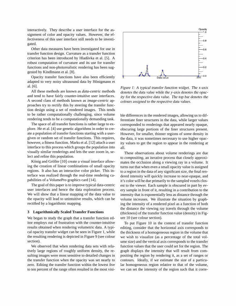
Transfer functions are often manually created usingan editable graph, relating the original data values onthe horizontal axes to associated opacities on the verti-cal axis. This paper addresses the vertical scale on thiseditable graph, and presents the advantages of using alogarithmic scale instead of the usual linear one.

After a review of current transfer function approachesin Section 2, Section 3 provides the motivation behindusing a logarithmic scale to specify transfer functions.In Section 4 we compare images produced using trans-fer functions specified on a linear scale with images pro-duced using transfer functions specified on a logarithmicscale. Section 5 summarizes our results and looks at pos-sible future work.

2 Previous Work

Transfer functions are an essential part of the volume ren-dering pipeline. Drebin et al. [3] have been using themin order to assign material percentages to the given datavalues. Levoy [11] used the data value and its derivativemagnitude in order to visualize boundaries of equal thick-ness or strength. Since these methods (also classified asdata-centric) are not intuitive to use, several researchershave tried to enhance the user interfaces in order to makedata exploration more effective.

Recently the concept of material percentage volumehas been extended by Bergner et al. [2] using spectraltransfer functions and a user interface based on a light-dial in order to explore various parameter combinations.

Bajaj et al. [1] compute several isosurface metrics ofthe data, such as the enclosed area or volume as well asthe gradient surface integral for the selected iso-value.These metrics serve as a guide for selecting iso-valuesor more complex transfer functions. The hope is that theminima or maxima of these curves represent interestingplaces in the data that are worth visualizing. This is alsoknown as the contour spectrum. Pekar et al. [13] suggestLaplacian-weighted histograms that compute the gradi-ent magnitude over the isosurface, indicating strong tran-sition regions at its maxima. They use the divergencetheorem in order to compute the histograms efficiently.

Kindlmann et al. [7] suggest the use of 2D histogramsof the gradient magnitude as well as the second deriva-tive of the data in the direction of the gradient. They ar-gue that within transition regions the shape of these his-tograms takes on a particular arch-like structure, whichcan be used to guide the user to find interesting transi-tion regions in the data. They further suggest the semi-automatic creation of transfer functions, where the usersimply inputs a surface distance to opacity map in or-der to visualize the data. This idea has been extendedby Tenginakai et al. [15] using a more general statisticalapproach using localized k-order central moments.

Kniss et al. [9] suggest a local probing of the underly-ing data which uses the 2D histograms of Kindlmann etal. [7] in order to find boundary regions within the data

interactively. They describe a user interface for the as-signment of color and opacity values. However, the ef-fectiveness of this user interface still needs to be investi-gated.

Other data measures have been investigated for use intransfer function design. Curvature as a transfer functioncriterion has been introduced by Hladuvka et al. [5]. Arobust computation of curvature and its use for transferfunctions and non-photorealistic rendering has been sug-gested by Kindlmann et al. [8].

Opacity transfer functions have also been efficientlyadapted to very noisy ultrasound data by Honigmann etal. [6].

All these methods are known asdata-centricmethodsand tend to have fairly counter-intuitive user interfaces.A second class of methods known asimage-centricap-proaches try to rectify this by steering the transfer func-tion design using a set of rendered images. This tendsto be rather computationally challenging, since volumerendering tends to be a computationally demanding task.

The space of all transfer functions is rather large to ex-plore. He et al. [4] use genetic algorithms in order to cre-ate a population of transfer functions starting with a user-given or random set of transfer functions. This requires,however, a fitness function. Marks et al. [12] attach a userinterface to this process which groups the population intovisually similar renderings and lets the user zoom in, se-lect and refine this population.

Konig and Groller [10] create a visual interface allow-ing the creation of linear combinations of small opacityregions. It also has an interactive color picker. This in-terface was realized through the real-time rendering ca-pabilities of a VolumePro graphics card [14].

The goal of this paper is to improve typical data-centricuser interfaces and hence the data exploration process.We will show that a linear mapping of the data value tothe opacity will lead to unintuitive results, which can berectified by a logarithmic mapping.

3 Logarithmically Scaled Transfer Functions

We began to study the graph that a transfer function ed-itor employs out of frustration with the counter-intuitiveresults obtained when rendering volumetric data. A typi-cal opacity transfer widget can be seen in Figure 1, whilethe resulting rendering is depicted in Figure 9 (see coloursection).

We observed that when rendering data sets with rela-tively large regions of roughly uniform density, the re-sulting images were most sensitive to detailed changes inthe transfer function when the opacity was set nearly tozero. Editing the transfer function within the lowest fiveto ten percent of the range often resulted in the most visi-

Figure 1: A typical transfer function widget. The x-axisdenotes the data value while the y-axis denotes the opac-ity for the respective data value. The top bar denotes thecolours assigned to the respective data values.

ble differences in the rendered images, allowing us to dif-ferentiate finer structures in the data, while larger valuescorresponded to renderings that appeared nearly opaque,obscuring large portions of the finer structures present.However, for smaller, thinner regions of some density inthe data, it was sometimes necessary to use higher opac-ity values to get the region to appear in the rendering atall.

These observations about volume renderings are dueto compositing, an iterative process that closely approxi-mates the occlusion along a viewing ray in a volume. Itturns out that when even a small opacity value is assignedto a region in the data of any significant size, the final ren-dered intensity will quickly increase to near-opaque, andit’s color will be due primarily to the sampled voxels clos-est to the viewer. Each sample is obscured in part by ev-ery sample in front of it, resulting in a contribution to theintensity that is exponentially less as distance through thevolume increases. We illustrate the situation by graph-ing the intensity of a rendered pixel as a function of boththe distance the viewing ray travels through the volume(thickness) of the transfer function value (density) in Fig-ure 10 (see colour section).

To put Figure 10 in the context of transfer functionediting, consider that the horizontal axis corresponds tothe thickness of a homogeneous region in the volume thatwe wish to visualize (as a percentage of the total vol-ume size) and the vertical axis corresponds to the transferfunction values that the user could set for the region. Thegraph displays the intensity that will result from com-positing the region by rendering it, as a set of ranges orcontours. Ideally, if we estimate the size of a particu-lar homogeneous region relative to that of the volume,we can set the intensity of the region such that it corre-

sponds to any one of the intensities on the graph that wedesire. The apparent difficulty is that most of the bandsof intensity on the graph are very narrow and are highlydependent on the size of the region in question.

The fact that the bands span an extremely narrow re-gion for depths above 30 percent of the volume meansthat for such regions, differences in transfer function val-ues as small as 0.001 (in the region near zero) will visiblychange the image. Even if an entire screen is used fora transfer function editor, a user must be able to spec-ify transfer functions to the accuracy of a single pixel tomake such changes. At the same time, values above 0.05all map to nearly opaque, resulting in 95 percent of thescreen space being wasted.

We propose a better approach by observing that we canscale the vertical axis of the graph in any way we wish,though the horizontal axis scale is fixed by the render-ing method (alpha compositing). If we scale the transferfunction opacities logarithmically, the result is a graphas in Figure 11 (see colour section). In this graph, theregions of intensity are better distributed, without ”push-ing” any of them off of the graph. Consequently, it wouldbe easier, both conceptually and physically, for a user toprecisely control the intensity of a region in the volume.This should result in more efficient transfer function edit-ing, which is significant since transfer function editing isone of the most time-consuming aspects of creating clearand informative renderings of medical, mathematical orgenerally scientific data sets.

Naturally, one can convert a linear transfer functionview into a logarithmically one quite easily. If we denotewith d the dimension of the data set, then letρd representthe “optical density” (transparency) of the data set, whiledα would represent the corresponding “physical thick-ness” of the data set. Adjusting for a bijective mappingfrom the interval[0, 1] onto and into itself, we can de-rive the following relationship between the linearly scaledopacity transfer functionα of Figure 10 and the logarith-mically scaled opacity transfer functionα′ of Figure 11(see colour section):

(ρα′)d = dα′

= dα + (1.0− α) (1)

This assumes an assignment of an “optical density” fora particular material ofρ = ( d

√d)α′

, which can be con-sidered a user controlled parameter. The above equationcan be expressed as

α′ = 1.0− 1−a

ln((1− e−a)α + e−a) (2)

Whereα′ is the scaled transfer function value obtainedfrom α, the transfer function value, and

a = max(ln d, 1) (3)

To map a point on the logarithmic graph back to atransfer function value (which is necessary during inter-active editing) the inverse transformation is used:

α =e−a(1−α′) − e−a

1− e−a(4)

whereα is the transfer function value obtained fromα′,the logarithmically scaled value from the graph. Themain logarithmic mapping isα = e−a(1−α′), wherea is auser controlled parameter. Equation 4 results by ensuringa bijective mapping from the interval[0, 1] onto and intoitself.

4 Results

Here we present renderings of a data sets using the tradi-tional (linear) opacity transfer functions in comparison toour new logarithmically scaled opacity transfer functions.

We start with a synthetic data set which illustratesthe problem nicely. Our data set consists of concentricspheres generated by the following function

f(x, y, z) = max(0, 1− d2n

d

√x2 + y2 + z2e/n) (5)

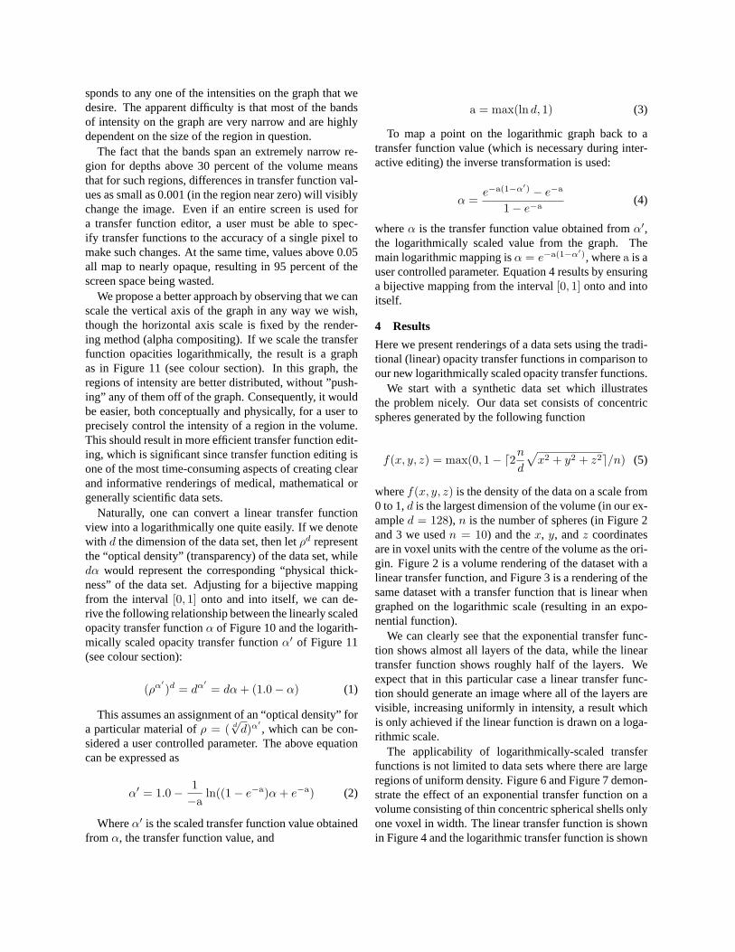
wheref(x, y, z) is the density of the data on a scale from0 to 1,d is the largest dimension of the volume (in our ex-ampled = 128), n is the number of spheres (in Figure 2and 3 we usedn = 10) and thex, y, andz coordinatesare in voxel units with the centre of the volume as the ori-gin. Figure 2 is a volume rendering of the dataset with alinear transfer function, and Figure 3 is a rendering of thesame dataset with a transfer function that is linear whengraphed on the logarithmic scale (resulting in an expo-nential function).

We can clearly see that the exponential transfer func-tion shows almost all layers of the data, while the lineartransfer function shows roughly half of the layers. Weexpect that in this particular case a linear transfer func-tion should generate an image where all of the layers arevisible, increasing uniformly in intensity, a result whichis only achieved if the linear function is drawn on a loga-rithmic scale.

The applicability of logarithmically-scaled transferfunctions is not limited to data sets where there are largeregions of uniform density. Figure 6 and Figure 7 demon-strate the effect of an exponential transfer function on avolume consisting of thin concentric spherical shells onlyone voxel in width. The linear transfer function is shownin Figure 4 and the logarithmic transfer function is shown

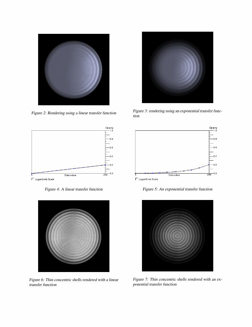
Figure 2: Rendering using a linear transfer function Figure 3: rendering using an exponential transfer func-tion

Figure 4: A linear transfer function Figure 5: An exponential transfer function

Figure 6: Thin concentric shells rendered with a lineartransfer function

Figure 7: Thin concentric shells rendered with an ex-ponential transfer function

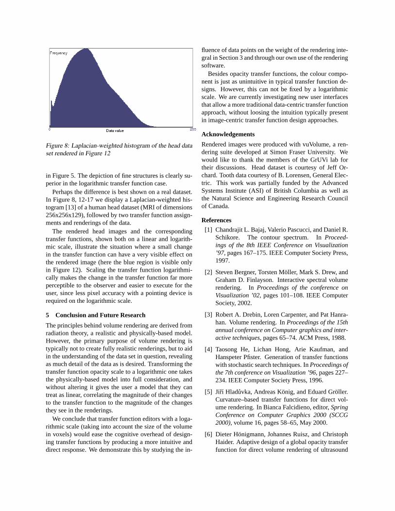
Figure 8: Laplacian-weighted histogram of the head dataset rendered in Figure 12

in Figure 5. The depiction of fine structures is clearly su-perior in the logarithmic transfer function case.

Perhaps the difference is best shown on a real dataset.In Figure 8, 12-17 we display a Laplacian-weighted his-togram [13] of a human head dataset (MRI of dimensions256x256x129), followed by two transfer function assign-ments and renderings of the data.

The rendered head images and the correspondingtransfer functions, shown both on a linear and logarith-mic scale, illustrate the situation where a small changein the transfer function can have a very visible effect onthe rendered image (here the blue region is visible onlyin Figure 12). Scaling the transfer function logarithmi-cally makes the change in the transfer function far moreperceptible to the observer and easier to execute for theuser, since less pixel accuracy with a pointing device isrequired on the logarithmic scale.

5 Conclusion and Future Research

The principles behind volume rendering are derived fromradiation theory, a realistic and physically-based model.However, the primary purpose of volume rendering istypically not to create fully realistic renderings, but to aidin the understanding of the data set in question, revealingas much detail of the data as is desired. Transforming thetransfer function opacity scale to a logarithmic one takesthe physically-based model into full consideration, andwithout altering it gives the user a model that they cantreat as linear, correlating the magnitude of their changesto the transfer function to the magnitude of the changesthey see in the renderings.

We conclude that transfer function editors with a loga-rithmic scale (taking into account the size of the volumein voxels) would ease the cognitive overhead of design-ing transfer functions by producing a more intuitive anddirect response. We demonstrate this by studying the in-

fluence of data points on the weight of the rendering inte-gral in Section 3 and through our own use of the renderingsoftware.

Besides opacity transfer functions, the colour compo-nent is just as unintuitive in typical transfer function de-signs. However, this can not be fixed by a logarithmicscale. We are currently investigating new user interfacesthat allow a more traditional data-centric transfer functionapproach, without loosing the intuition typically presentin image-centric transfer function design approaches.

Acknowledgements

Rendered images were produced with vuVolume, a ren-dering suite developed at Simon Fraser University. Wewould like to thank the members of the GrUVi lab fortheir discussions. Head dataset is courtesy of Jeff Or-chard. Tooth data courtesy of B. Lorensen, General Elec-tric. This work was partially funded by the AdvancedSystems Institute (ASI) of British Columbia as well asthe Natural Science and Engineering Research Councilof Canada.

References

[1] Chandrajit L. Bajaj, Valerio Pascucci, and Daniel R.Schikore. The contour spectrum. InProceed-ings of the 8th IEEE Conference on Visualization’97, pages 167–175. IEEE Computer Society Press,1997.

[2] Steven Bergner, Torsten Moller, Mark S. Drew, andGraham D. Finlayson. Interactive spectral volumerendering. InProceedings of the conference onVisualization ’02, pages 101–108. IEEE ComputerSociety, 2002.

[3] Robert A. Drebin, Loren Carpenter, and Pat Hanra-han. Volume rendering. InProceedings of the 15thannual conference on Computer graphics and inter-active techniques, pages 65–74. ACM Press, 1988.

[4] Taosong He, Lichan Hong, Arie Kaufman, andHanspeter Pfister. Generation of transfer functionswith stochastic search techniques. InProceedings ofthe 7th conference on Visualization ’96, pages 227–234. IEEE Computer Society Press, 1996.

[5] Jirı Hladuvka, Andreas Konig, and Eduard Groller.Curvature–based transfer functions for direct vol-ume rendering. In Bianca Falcidieno, editor,SpringConference on Computer Graphics 2000 (SCCG2000), volume 16, pages 58–65, May 2000.

[6] Dieter Honigmann, Johannes Ruisz, and ChristophHaider. Adaptive design of a global opacity transferfunction for direct volume rendering of ultrasound

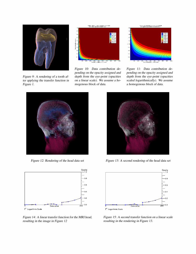
Figure 9: A rendering of a tooth af-ter applying the transfer function inFigure 1.

Figure 10: Data contribution de-pending on the opacity assigned anddepth from the eye-point (opacitieson a linear scale). We assume a ho-mogenous block of data.

Figure 11: Data contribution de-pending on the opacity assigned anddepth from the eye-point (opacitiesscaled logarithmically). We assumea homogenous block of data.

Figure 12: Rendering of the head data set Figure 13: A second rendering of the head data set

Figure 14: A linear transfer function for the MRI head,resulting in the image in Figure 12

Figure 15: A second transfer function on a linear scaleresulting in the rendering in Figure 13.

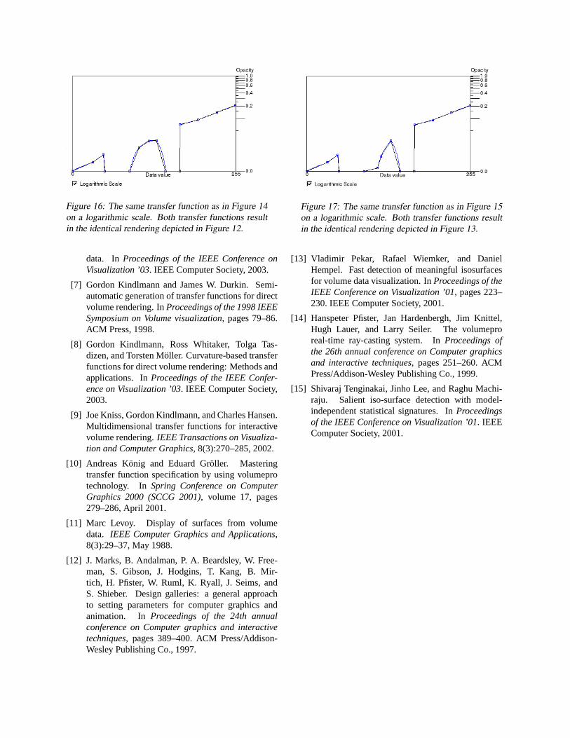
Figure 16: The same transfer function as in Figure 14on a logarithmic scale. Both transfer functions resultin the identical rendering depicted in Figure 12.

Figure 17: The same transfer function as in Figure 15on a logarithmic scale. Both transfer functions resultin the identical rendering depicted in Figure 13.

data. InProceedings of the IEEE Conference onVisualization ’03. IEEE Computer Society, 2003.

[7] Gordon Kindlmann and James W. Durkin. Semi-automatic generation of transfer functions for directvolume rendering. InProceedings of the 1998 IEEESymposium on Volume visualization, pages 79–86.ACM Press, 1998.

[8] Gordon Kindlmann, Ross Whitaker, Tolga Tas-dizen, and Torsten Moller. Curvature-based transferfunctions for direct volume rendering: Methods andapplications. InProceedings of the IEEE Confer-ence on Visualization ’03. IEEE Computer Society,2003.

[9] Joe Kniss, Gordon Kindlmann, and Charles Hansen.Multidimensional transfer functions for interactivevolume rendering.IEEE Transactions on Visualiza-tion and Computer Graphics, 8(3):270–285, 2002.

[10] Andreas Konig and Eduard Groller. Masteringtransfer function specification by using volumeprotechnology. InSpring Conference on ComputerGraphics 2000 (SCCG 2001), volume 17, pages279–286, April 2001.

[11] Marc Levoy. Display of surfaces from volumedata. IEEE Computer Graphics and Applications,8(3):29–37, May 1988.

[12] J. Marks, B. Andalman, P. A. Beardsley, W. Free-man, S. Gibson, J. Hodgins, T. Kang, B. Mir-tich, H. Pfister, W. Ruml, K. Ryall, J. Seims, andS. Shieber. Design galleries: a general approachto setting parameters for computer graphics andanimation. In Proceedings of the 24th annualconference on Computer graphics and interactivetechniques, pages 389–400. ACM Press/Addison-Wesley Publishing Co., 1997.

[13] Vladimir Pekar, Rafael Wiemker, and DanielHempel. Fast detection of meaningful isosurfacesfor volume data visualization. InProceedings of theIEEE Conference on Visualization ’01, pages 223–230. IEEE Computer Society, 2001.

[14] Hanspeter Pfister, Jan Hardenbergh, Jim Knittel,Hugh Lauer, and Larry Seiler. The volumeproreal-time ray-casting system. InProceedings ofthe 26th annual conference on Computer graphicsand interactive techniques, pages 251–260. ACMPress/Addison-Wesley Publishing Co., 1999.

[15] Shivaraj Tenginakai, Jinho Lee, and Raghu Machi-raju. Salient iso-surface detection with model-independent statistical signatures. InProceedingsof the IEEE Conference on Visualization ’01. IEEEComputer Society, 2001.