Transfer learning for class imbalance problems with ...dmkd.cs.vt.edu/papers/KAIS16.pdfTransfer learning for class imbalance problems with inadequate data ... training and the generalization

Knowl Inf Syst (2016) 48:201–228DOI 10.1007/s10115-015-0870-3

REGULAR PAPER

Transfer learning for class imbalance problemswith inadequate data

Samir Al-Stouhi1 · Chandan K. Reddy2

Received: 31 August 2014 / Revised: 30 May 2015 / Accepted: 2 August 2015 /Published online: 25 August 2015© Springer-Verlag London 2015

Abstract A fundamental problem in data mining is to effectively build robust classifiersin the presence of skewed data distributions. Class imbalance classifiers are trained specifi-cally for skewed distribution datasets. Existing methods assume an ample supply of trainingexamples as a fundamental prerequisite for constructing an effective classifier. However,when sufficient data are not readily available, the development of a representative classifica-tion algorithm becomes even more difficult due to the unequal distribution between classes.We provide a unified framework that will potentially take advantage of auxiliary data using atransfer learning mechanism and simultaneously build a robust classifier to tackle this imbal-ance issue in the presence of few training samples in a particular target domain of interest.Transfer learning methods use auxiliary data to augment learning when training examplesare not sufficient and in this paper we will develop a method that is optimized to simulta-neously augment the training data and induce balance into skewed datasets. We propose anovel boosting-based instance transfer classifier with a label-dependent update mechanismthat simultaneously compensates for class imbalance and incorporates samples from an aux-iliary domain to improve classification. We provide theoretical and empirical validation ofour method and apply to healthcare and text classification applications.

Keywords Rare class · Transfer learning · Class imbalance · AdaBoost · Weighted majorityalgorithm · HealthCare informatics · Text mining

1 Introduction

One of the fundamental problems in machine learning is to effectively build robust classifiersin the presence of class imbalance. Imbalanced learning is a well-studied problem and many

B Chandan K. [email protected]

1 Honda Automobile Technology Research, Southfield, MI, USA

2 Department of Computer Science, Wayne State University, Detroit, MI, USA

123

http://crossmark.crossref.org/dialog/?doi=10.1007/s10115-015-0870-3&domain=pdf

202 S. Al-Stouhi, C. K. Reddy

sampling techniques, cost-sensitive algorithms, kernel-based techniques, and active learningmethods have been proposed in the literature [1]. Though there have been several attempts tosolve this problem, most of the existing methods always assume an ample supply of trainingexamples as a fundamental prerequisite for constructing an effective classifier tackling classimbalance problems. In otherwords, the existing imbalanced learning algorithmsonly addressthe problemof “Relative Imbalance”where the number of samples in one class is significantlyhigher compared to the other class and there is an abundant supply of training instances.However, when sufficient data for model training is not readily available, the developmentof a representative hypothesis becomes more difficult due to an unequal distribution betweenits classes.

Many datasets related to medical diagnoses, natural phenomena, or demographics are nat-urally imbalanced datasets and will typically have an inadequate supply of training instances.For example, datasets for cancer diagnosis in minority populations (benign or malignant), orseismic wave classification datasets (earthquake or nuclear detonation) are small and imbal-anced. “Absolute Rarity” refers to a dataset where the imbalance problem is compounded bya supply of training instances that is not adequate for generalization. Many of such practicaldatasets have high dimensionality, small sample size and class imbalance. The minority classwithin a small and imbalanced dataset is considered to be a “Rare Class”. Classificationwith “Absolute Rarity” is not a well-studied problem because the lack of representative data,especially within the minority class, impedes learning.

To address this challenge, we develop an algorithm to simultaneously rectify for the skewwithin the label space and compensate for the overall lack of instances in the training set byborrowing from an auxiliary domain. We provide a unified framework that can potentiallytake advantage of the auxiliary data using a “knowledge transfer” mechanism and build arobust classifier to tackle this imbalance issue in the presence of fewer training samples inthe target domain. Transfer learning algorithms [2,3] use auxiliary data to augment learningwhen training examples are not sufficient. In the presence of inadequate number of samples,the transfer learning algorithms will improve learning on a small dataset (referred to as targetset) by including a similar and possibly larger auxiliary dataset (referred to as the sourceset). In this work, we will develop one such method optimized to simultaneously augmentthe training data and induce balance into the skewed datasets.

This paper presents the first method for rare dataset classification within a transfer learn-ing paradigm. In this work, we propose a classification algorithm to address the problem of“Absolute Rarity” with an instance transfer method that incorporates the best-fit set of aux-iliary samples that improve balanced error minimization. Our transfer learning frameworkinduces balanced error optimization by simultaneously compensating for the class imbal-ance and the lack of training examples in “Absolute Rarity”. To achieve this goal, we utilizeensemble-learning techniques that iteratively construct a classifier that is trained with theweighted source and target samples that best improve balanced classification. Our transferlearning algorithm will include label information while performing knowledge transfer.

This paper effectively combines two important machine learning concepts: the concept ofcompensating for the skew within the label space (which belongs to the domain of “Imbal-anced Learning”) and the concept of extracting knowledge from an auxiliary dataset tocompensate for the overall lack of samples (which belongs to a family of methods known as“instance-based transfer learning”). We aim to construct a hypothesis and uncover the sepa-rating hyperplane with only a handful of training examples with data that is complex in boththe feature and label spaces. The complexity of the data skewness and the rarity of trainingexamples prohibit hypothesis construction by human experts or standard algorithms, and thus

123

Transfer learning for class imbalance problems with. . . 203

we present a solution that can be applied when nothing else suffices. The main contributionsof this paper are as follows:

1. Present a complete categorization of several recent works and highlight the need for anew type of specialized algorithms to solve a niche but important problem that is notaddressed in the current literature.

2. Propose a novel transfer learning algorithm, Rare-Transfer, optimized for transfer withinthe label space to effectively handle rare class problems.

3. Provide theoretical and empirical analysis of the proposed Rare-Transfer algorithm.4. Demonstrate the superior performance of the proposed algorithm compared to several

existing methods in the literature using various real-world examples.

The rest of the paper is organized as follows: In Sect. 2, we describe the different typesof datasets and briefly discuss the related methods suitable for each type. Section 3 presentsthe motivation for a unified balanced optimization framework. Section 4 describes our algo-rithm, “Rare-Transfer”, which addresses the “Absolute Rarity” problem. Section 5 presentsthe theoretical analysis of the proposed algorithm. For further validation, Sect. 6 presentsempirical analysis of our framework and is followed by experimental results on real-worlddata in Sect. 7. Finally, we discuss possible extensions and conclude our work.

2 Characterization of existing machine learning domains

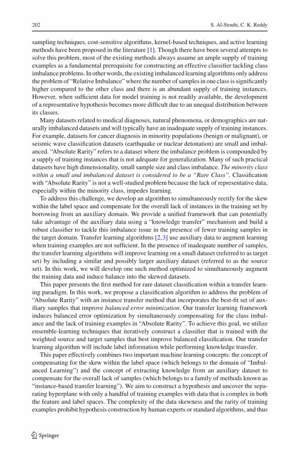
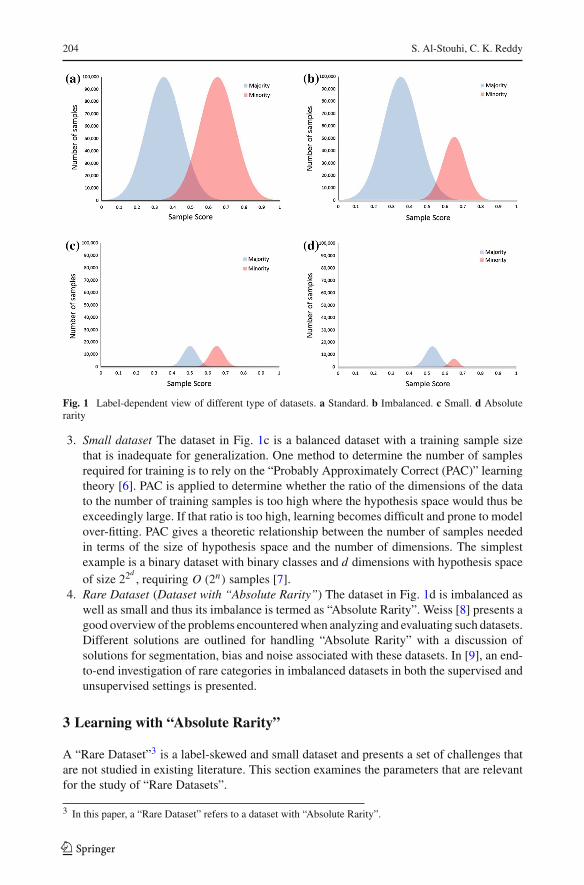
To describe datasets in terms of both size and imbalance, we use the “Label-Dependent” viewin Fig. 1. The sub-figures present a binary classification problem with normally distributedsamples within each class1 (thus we describe it as label-dependent since the distributions arenormal within each label). Figure 1 illustrates the different datasets with an overview of therelated machine learning fields2 that can improve learning.

1. Standard dataset Figure 1a depicts a standard dataset with a relatively equal number ofsamples within each class (balanced class distribution) and an adequate number of sam-ples for generalization. To learn from balanced datasets, equal importance is assigned toall classes and thusmaximizing the overall arithmetic accuracy is the chosen optimizationobjective. A variety of standard machine learning and data mining approaches can beapplied for standard datasets as such methods serve as the foundation for the algorithmsthat are modified for any peculiar feature set or distribution.

2. Imbalanced dataset The dataset in Fig. 1b is a relatively imbalanced dataset. It is rela-tively imbalanced because there is a between-class imbalancewhere one class encompassthe majority of the training set. The balance is relative since both minority and majoritytraining subsets contain adequate training samples. For example, email spam classifica-tion is a relatively imbalanced problem since 97% (majority) of emails sent over the netare considered unwanted emails [4] and with around 200 billion messages of spam sentper day [5], the number of non-spam emails (minority) is also a large dataset. A datasetwhere the number samples belonging to different classes is highly disproportionate isconsidered to be an “imbalanced dataset” with the postulation that the imbalance is rela-tive [1]. Because the majority class overwhelms the minority class, imbalanced learningmodels are biased to improve learning on the minority class (without any considerationto the availability of training examples).

1 The terms class and label are used interchangeably in our discussion.2 Only concepts that are relevant for “Absolute Rarity” are discussed.

123


Fig. 1 Label-dependent view of different type of datasets. a Standard. b Imbalanced. c Small. d Absoluterarity

3. Small dataset The dataset in Fig. 1c is a balanced dataset with a training sample sizethat is inadequate for generalization. One method to determine the number of samplesrequired for training is to rely on the “Probably Approximately Correct (PAC)” learningtheory [6]. PAC is applied to determine whether the ratio of the dimensions of the datato the number of training samples is too high where the hypothesis space would thus beexceedingly large. If that ratio is too high, learning becomes difficult and prone to modelover-fitting. PAC gives a theoretic relationship between the number of samples neededin terms of the size of hypothesis space and the number of dimensions. The simplestexample is a binary dataset with binary classes and d dimensions with hypothesis spaceof size 22

d, requiring O (2n) samples [7].

4. Rare Dataset (Dataset with “Absolute Rarity”) The dataset in Fig. 1d is imbalanced aswell as small and thus its imbalance is termed as “Absolute Rarity”. Weiss [8] presents agood overview of the problems encounteredwhen analyzing and evaluating such datasets.Different solutions are outlined for handling “Absolute Rarity” with a discussion ofsolutions for segmentation, bias and noise associated with these datasets. In [9], an end-to-end investigation of rare categories in imbalanced datasets in both the supervised andunsupervised settings is presented.

3 Learning with “Absolute Rarity”

A “Rare Dataset”3 is a label-skewed and small dataset and presents a set of challenges thatare not studied in existing literature. This section examines the parameters that are relevantfor the study of “Rare Datasets”.

3 In this paper, a “Rare Dataset” refers to a dataset with “Absolute Rarity”.

123


3.1 Effect of data size on learning

3.1.1 Balanced dataset

The first impediment to learning with “Absolute Rarity” is the fact that the small size ofthe training set, regardless of imbalance, impedes learning. When the number of trainingexamples is not adequate to generalize to instances not present in the training data, it is nottheoretically possible to use a learning model as the model will only overfit the training set.The term “adequate” is a broad term as many factors including data complexity, number ofdimensions, data duplication, and overlap complexity have to be considered [1]. Computa-tional learning theory [7] provides a general outline to estimate the difficulty of learning amodel, the required number of training examples, the expected learning and generalizationerror and the risk of failing to learn or generalize.

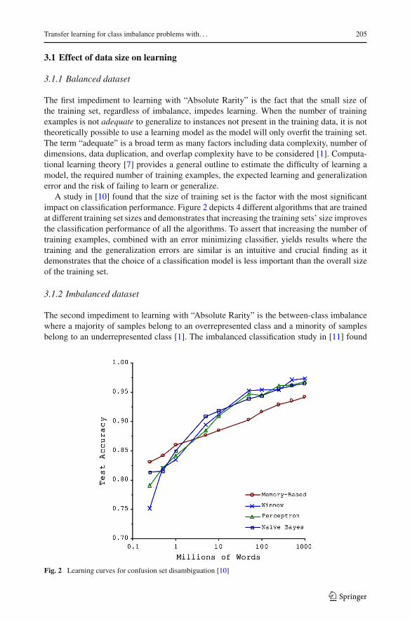
A study in [10] found that the size of training set is the factor with the most significantimpact on classification performance. Figure 2 depicts 4 different algorithms that are trainedat different training set sizes and demonstrates that increasing the training sets’ size improvesthe classification performance of all the algorithms. To assert that increasing the number oftraining examples, combined with an error minimizing classifier, yields results where thetraining and the generalization errors are similar is an intuitive and crucial finding as itdemonstrates that the choice of a classification model is less important than the overall sizeof the training set.

3.1.2 Imbalanced dataset

The second impediment to learning with “Absolute Rarity” is the between-class imbalancewhere a majority of samples belong to an overrepresented class and a minority of samplesbelong to an underrepresented class [1]. The imbalanced classification study in [11] found

Fig. 2 Learning curves for confusion set disambiguation [10]

123


Fig. 3 AUC for imbalanced datasets at different training sample sizes [11]. a Adult. b Covertype

that the most significant effect on a classifier’s performance in an imbalanced classificationproblem is not the ratio of imbalance, but it is the number of samples in the training set. Thisis an important finding as it demonstrates that the lack of data in “Absolute Rarity” intensifiesthe label imbalance problem. As the number of the training examples increased, the errorrate caused by imbalance decreased [12] and thus increasing the number of training samplesmakes the classifiers less sensitive to the between-class imbalance [11].

Figure 3 demonstrates how the lack of training examples degrades learning in an imbal-anced dataset [11]. The ROC curve illustrates the performance of a binary classifier wherethe x-axis represents the False Positive Rate (1-Specificity) and the y-axis represents the TruePositive Rate and is an accepted metric in imbalanced learning problems. Figure 3 presentsthe Area Under the ROC curve (AUC) [13] results in [11] where a classifier was trainedfor two imbalanced datasets [14] with different subsets of training sets (with a total of nsamples). AUC is a simple summary of the ROC performance and can be calculated by usingthe trapezoidal areas created between ROC points and is thus equivalent to the Wilcoxon–Mann–Whitney statistic [15]. The results demonstrate that increasing the size of the trainingset directly improves learning for imbalanced datasets.

4 The proposed rare-transfer algorithm

4.1 Notations

Consider a domain (D) comprised of instances (X ∈ Rd) with d features. We can specify

a mapping function, F , to map the feature space to the label space as “X → Y ” whereY ∈ {−1, 1}. If no source or target instances are defined, then n will simply refer to thenumber of instances in a dataset; otherwise, we will denote the domain with n auxiliaryinstances as the source domain (Dsrc) and define (Dtar ) as the target domain with m � ninstances. Instances that belong to themajority class will be defined as Xmajority and those thatbelong to the minority class will be defined as Xminority. nl is the number of source samplesthat belong to label l, while εl is the error rate for label l and denotes the misclassificationrate for samples with true label l. N defines the total number of boosting iterations, w is a

weight vector. A weak classifier at a given boosting iteration (t) will be defined as..

f t , andits classification error is denoted by εt . I is an indicator function and is defined as:

123


I[y �= f̈

] ={1 y �= f̈0 y = f̈

(1)

4.2 Boosting-based transfer learning

Boosting-based transfer learning algorithms apply ensemble methods to both source andtarget instances with an update mechanism that incorporates only the source instances thatare useful for target instance classification. These methods perform this form of mappingby giving more weight to source instances that improve target training and decreasing theweights for instances that induce negative transfer.

TrAdaBoost [16] is the first and most popular transfer learning method that uses boostingas a best-fit inductive transfer learner. TrAdaBoost trains a base classifier on the weightedsource and target set in an iterative manner. After every boosting iteration, the weights ofmisclassified target instances are increased and the weights of correctly classified targetinstances are decreased. This target update mechanism is based solely on the training errorcalculated on the normalized weights of the target set and uses a strategy adapted from theclassical AdaBoost [17] algorithm. The weighted majority algorithm (WMA) [18] is usedto adjust the weights of the source set by iteratively decreasing the weight of misclassifiedsource instances by a constant factor and preserving the current weights of correctly classifiedsource instances. The basic idea is that the weight of source instances that are not correctlyclassified on a consistent basis would converge and would not be used in the final classifier’soutput since that classifier only uses boosting iterations N

2 → N for convergence [16].TrAdaBoost has been extended to many transfer learning problems. A multi-source learn-

ing [19] approach was proposed to import knowledge from many sources. Having multiplesources increases the probability of integrating source instances that are better fit to improvetarget learning and thus this method can reduce negative transfer. A model-based transferin “TaskTrAdaBoost” [19] extends this algorithm to transferring knowledge from multiplesource tasks to learn a specific target task. Since closely related tasks share some commonparameters, suitable parameters that induce positive transfer are integrated from multiplesource tasks. Some of the prominent applications of TrAdaBoost include multi-view surveil-lance [19], imbalanced classification [20], head-pose estimation [21], visual tracking [22],text classification [16] and several other problems [2].

TransferBoost [23] is an AdaBoost based method for boosting when multiple source tasksare available. It boosts all source weights for instances that belong to tasks exhibiting positivetransferability to the target task. TransferBoost calculates an aggregate transfer term for everysource task as the difference in error between the target-only task and the target plus eachadditional source task. AdaBoost was extended in [24] for concept drift as a fixed cost ispre-calculated using Euclidean distance (as one of two options) as a measure of relevancebetween source and target distributions. This relevance ratio thus gives more weights to datathat is near in the feature space and share a similar label. This ratio is finally incorporated tothe update mechanism via AdaCost [25].

Many problems have been noted when using TrAdaBooost. The authors in [26] reportedthat there was a weight mismatch when the size of source instances is much larger than thatof target instances. This required many iterations for the total weight of the target instancesto approach that of the source instances. In [27], it was noted that TrAdaBoost yielded afinal classifier that always predicted one label for all instances as it substantially unbalancedthe weights between the different classes. Even the original implementation of TrAdaBoostin [16] re-sampled the data at each step to balance the classes. Finally, various researchersobserved that beneficial source instances that are representative of the target concept tend

123


to have a quick and stochastic weight convergence. This quick convergence was examinedby Eaton and desJardins [23] as they observed that in TrAdaBoost’s reweighing scheme,the difference between the weights of the source and target instances only increased andthat there was no mechanism in place to recover the weight of source instances in laterboosting iterations when they become beneficial. TrAdaBoost was improved in [28] wheredynamic reweighing separated the two update mechanisms of AdaBoost andWMA for betterclassification performance.

4.3 The proposed rare-transfer algorithm

To overcome the limitations in boosting-based transfer learning and simultaneouslyaddress imbalance in “Absolute Rarity”, we present the “Rare-Transfer” algorithm (shownin Algorithm 1). The algorithm exploits transfer learning concepts to improve classificationby incorporating auxiliary knowledge from a source domain to a target domain. Simultane-

Algorithm 1 Rare-Transfer AlgorithmRequire:

• Source domain instances Dsrc = {(xsrci , ysrci

)}

• Target domain instances Dtar = {(xtari , ytari

)}

• Maximum number of iterations : N

• Base learner : ..f

Ensure: Target Classifier Output :{ .

f : X → Y}

.f = sign

⎡

⎢⎣

N∏

t= N2

(

βttar

−..

f t)

−N∏

t= N2

(

βttar

− 12

)⎤

⎥⎦

Procedure:1: Initialize the weights w for all instances D = {Dsrc ∪ Dtar }, where:

wsrc = {wsrc1 , . . . , wsrcn

}, wtar = {wtar1 , . . . , wtarm

}, w = {wsrc ∪ wtar }

2: Set βsrc = 1

1+√

2 ln(n)N

3: for t = 1 to N do4: Normalize Weights: w = w∑n

i wsrci +∑mj wtar j

5: Find the candidate weak learner..

f t : X → Y that minimizes error for D weighted according to w

6: Calculate the error of..

f t on Dsrc: εtsrc =∑n

j=1

[w

jsrc

]·I[

ysrc j �=..

f tj

]

∑ni=1

[wi

src

]

7: Calculate the error of..

f t on Dtar : εttar =∑m

j=1

[w

jtar

]·I[

ytar j �=..

f tj

]

∑mi=1

[wi

tar

]

8: Set Cl =(1 − εl

src

)

9: Set βtar = 1 − εttar

εttar

10: wt+1srci = Clwt

srciβ

I

[ysrci �=

..

f ti

]

src where i ∈ Dsrc

11: wt+1tar j

= wttar j

β

I

[ytar j �=

..

f tj

]

tar where j ∈ Dtar

12: end for

123


ously, balanced classification is improved as the algorithm allocates higher weights to thesubset of auxiliary instances that improve and balance the final classifier. The frameworkeffectively combines the power of two boosting algorithms with AdaBoost [17] updating thetarget instances’ weights and the weighted majority algorithm (WMA) [18], modified forbalanced transfer, updating the source instances’ weights to incorporate auxiliary knowledgeand skew for balanced classification via transfer from the source domain.

The two algorithms operate separately and are only linked in:

1. Line 4 (normalization): Both algorithms require normalization. The combined normal-ization causes an anomaly that we will address in subsequent analysis.

2. Line 5: Infusing source with target for training is how transfer learning is induced fromthe auxiliary dataset.

The target instances are updated in lines 7, 9, and 11 as outlined by AdaBoost [17]. The weaklearner in line 5 finds the separating hyperplane that forms the classification boundary and isused to calculate the target’s error rate

(εt

tar < 0.5)in line 7. This error is used in line 9 to

calculate (βtar > 1) which will then be used to update the target weights in line 11 as:

wt+1tar j

= wttar j

βI

[ytar j �=

..

f tj

]

tar (2)

Similar to AdaBoost, a misclassified target instance’s weight increases after normalizationandwould thus gainmore influence in the next iteration.Once boosting is completed, (t = N ),

the weak classifiers (..

f t ) weighted by βtar are combined to construct a committee capableof nonlinear approximation.

The source instances are updated in lines 2 and 10 as done by the weighted majorityalgorithm [18]. The static WMA update rate (βsrc < 1) is calculated on line 2 and updatesthe source weights as:

wt+1srci

= wtsrci

βI

[ysrci �=

..

f ti

]

src(3)

Contrary to AdaBoost, WMA decreases the influence of an instance that is misclassified andgives it a lower relative weight in the subsequent iterations. This property is beneficial fortransfer learning since the source instance’s contribution to the weak classifiers is dependenton its classification consistency. A consistently misclassified instance’s weight converges,4

and its influence diminishes in subsequent iterations. In Algorithm 1, the WMA updatemechanism in Eq. (3) is actually modified in line 10 to incorporate the cost Cl for label-dependent transfer. This dynamic cost is calculated in line 8, and it promotes balancedtransfer learning. Starting with equal initial weights and using standard weak classifiers thatoptimize for accuracy, these classifiers achieve low error rates for the majority and high errorrate for the minority as they are overwhelmed with the majority label. The label-dependentcost, Cl , controls the rate of convergence of the source instances and hence the weightsconverge slower5 for labels with high initial error rates (minority classes). As minority labelsget higher normalized weights with each successive boosting iteration, the weak classifierswould subsequently construct more balanced separating hyperplanes. The N

2 → N weakclassifiers are used for the final output with the expectation that the most consistent andbalanced mix of source instances would be used for learning the final classifier.

4 All mentions of “convergence” refer to a sequence (weight) that converges to zero.5 Slower or decreased convergence rate means that a weight converges to zero with higher number of boostingiterations.

123


5 Theoretical analysis of the rare-transfer algorithm

We will refer to the cost(Cl)on line 9 as the “Correction Factor” and prove in Sect. 5.1

that it prevents the source instances’ weights from early convergence. This improves transferlearning and addresses the lack of training data in a rare dataset. In Sect. 5.2, we providethe motivation for balanced optimization and modify this “Correction Factor” to incorporatebalanced optimization to simultaneously compensate for the lack of sufficient data and theclass imbalance within a rare dataset.

5.1 Correction for transfer learning

Definition 1 Given k instances at iteration t with normalized weight w and update rate β,the sum of the weights after one boosting iteration with error rate (εt ) is calculated as:

k∑

i=1

wt+1 = kwt (1 − εt ) + kwt (εt )β (4)

Wewill now explain this inmore detail with the help of an example. Given k = 10 instances atiteration t with normalized weights w = 0.1, assume that weak learner f̈ correctly classifies6 instances (εt = 0.4). Sum of correctly classified instances at boosting iteration t + 1 iscalculated as:

∑

y= f̈ t

wt+1 = 0.1β0 + 0.1β0 + 0.1β0 + 0.1β0 + 0.1β0 + 0.1β0

= 6(wt )β0 {since(wt = 0.1

)}

= 10(0.6)(wt )

= kwt (1 − εt ){since

(k = 10, εt = 0.4

)}(5)

On the other hand, the sum of misclassified instances at boosting iteration t + 1 is:∑

y �= f̈ t

wt+1 = 0.1β1 + 0.1β1 + 0.1β1 + 0.1β1

= 4(wt )β1 {since

(wt = 0.1

)}

= 10(0.4)(wt )β

= kwt (εt )β{since

(k = 10, εt = 0.4

)}(6)

Thus, the sum of weights at boosting iteration “t + 1” is calculated as:

k∑

i=1

wt+1 =∑

y= f̈ t

wt+1 +∑

y �= f̈ t

wt+1

= kwt (1 − εt ) + kwt (εt )β (7)

Proposition 1 All source instances are correctly classified by the weak learner:

ysrci = f̈ ti , ∀i ∈ {1, . . . , n} (8)

Equation (8) is analogous to:

n∑

i=1

wt+1 = nwtsrc

(1 − εt

src

)+ nwtsrc

(εt

src

)βsrc = nwt

src (9)

123


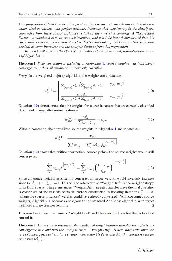
This proposition is held true in subsequent analysis to theoretically demonstrate that evenunder ideal conditions with perfect auxiliary instances that consistently fit the classifiers,knowledge from these source instances is lost as their weights converge. A “CorrectionFactor” is calculated to conserve such instances, and it will be later demonstrated that thiscorrection is inversely proportional to classifier’s error and approaches unity (no correctionneeded) as error increases and the analysis deviates from this proposition.

Theorem 1 will examine the effect of the combined (source + target) normalization in line4 of Algorithm 1.

Theorem 1 If no correction is included in Algorithm 1, source weights will improperlyconverge even when all instances are correctly classified.

Proof In the weighted majority algorithm, the weights are updated as:

wt+1src =

⎧⎪⎪⎪⎨

⎪⎪⎪⎩

wtsrc∑

{yi = fi } wtsrc+

∑{yi �= fi } βsrcwt

srcysrc =

..

f t

βsrcwtsrc∑

{yi = fi } wtsrc+

∑{yi �= fi } βsrcwt

srcysrc �=

..

f t

(10)

Equation (10) demonstrates that the weights for source instances that are correctly classifiedshould not change after normalization as:

wt+1src = wt

src∑ni=1 wt

srci

= wtsrc (11)

Without correction, the normalized source weights in Algorithm 1 are updated as:

wt+1src = wt

src

∑ni wt

srci+∑m

j wttar j

βI

[ytar j �=

..

f tj

]

tar

(12)

Equation (12) shows that, without correction, correctly classified source weights would stillconverge as:

m∑

j

wttar j

β

[ytar j �=

..

f tj

]

tar =m∑

j

wttar j

(1 − εt

tar

εttar

)I

[ytar j �=

..

f tj

]

(13)

Since all source weights persistently converge, all target weights would inversely increasesince (nwt

src + mwttar ) = 1. This will be referred to as “Weight Drift” since weight entropy

drifts from source to target instances. “Weight Drift” negates transfer since the final classifieris comprised of the cascade of weak learners constructed in boosting iterations N

2 → N(where the source instances’ weights could have already converged). With converged sourceweights, Algorithm 1 becomes analogous to the standard AdaBoost algorithm with targetinstances and no transfer learning. �Theorem 1 examined the cause of “Weight Drift” and Theorem 2 will outline the factors thatcontrol it.

Theorem 2 For n source instances, the number of target training samples (m) affects theconvergence rate and thus the “Weight Drift”. “Weight Drift” is also stochastic since therate of convergence at iteration t (without correction) is determined by that iteration’s targeterror rate (εt

tar ).

123


Proof The fastest rate6 of convergence is achieved by minimizing the weight for each sub-sequent boosting iteration (wt+1

src ) as:

minm,n,εt

tar

(wt+1

src

) = wtsrc

maxm,n,εt

tar

{∑n

i=1 wtsrci

+∑mj=1 wt

tar j

(1−εt

tarεt

tar

)I[

ytar j �=..

f tj

]} (14)

Equation (14) shows that two factors can slow down the rate of convergence of correctlyclassified source instances:

1. Maximizing the weak learner’s target error rate with εttar → 0.5 (choosing an extremely

weak learner or one that is only slightly better than random). Since the weak learner isweighted differently for each iteration, its error cannot be controlled and this factor willinduce a stochastic effect.

2. Decreasing the number of target samples m, since rate of convergence accelerates whenm/n → ∞. Attempting to slow the improper rate of convergence by reducing the numberof target instances is counterproductive as the knowledge from the removed instanceswould be lost. �

Theorem 2 demonstrated that a fixed cost cannot control the rate of convergence since thecumulative effect of m, n, and εt

tar is stochastic. A dynamic term has to be calculated tocompensate for “Weight Drift” at every iteration. The calculation of a dynamic term isoutlined in Theorem 3.

Theorem 3 A correction factor of 2(1 − εt

tar

)can be applied to the source weights to

prevent their “Weight Drift” and make the weights converge at a rate similar to that of theweighted majority algorithm.

Proof Un-wrapping the WMA source update mechanism of Eq. (14), yields:

wt+1src = wt

src

∑ni=1 wt

srci+∑m

j=1 wttar j

(1−εt

tarεt

tar

)I[

ytar j �=..

f tj

] = wtsrc

nwtsrc + A + B

(15)

where A and B are defined as:

A = Sum of correctly classified target weights at boosting iteration “t + 1”

= mwttar

(1 − εt

tar

)(16)

B = Sum of misclassified target weights at boosting iteration “t + 1”

= mwttar

(εt

tar

)β t

tar = mwttar

(εt

tar

) (1 − εttar

εttar

)I

[ytar j �=

..

f tj

]

= mwttar

(1 − εt

tar

)(17)

Substituting for A and B, the source update is:

wt+1src = wt

src

nwtsrc + 2mwt

tar(1 − εt

tar) (18)

6 Faster or increased convergence rate means that a weight converges to zero with lower number of boostingiterations.

123


We will introduce and solve for a correction factor Ct to equate (wt+1src = wt

src) for correctlyclassified instances (as per the WMA).

wtsrc = wt+1

src = Ctwtsrc

Ct nwtsrc + 2mwt

tar(1 − εt

tar) (19)

Solving for Ct :

Ct = 2mwttar

(1 − εt

tar

)

(1 − nwtsrc)

= 2mwttar

(1 − εt

tar

)

mwttar

= 2(1 − εt

tar

)(20)

�Adding this correction factor to line 10 of Algorithm 1 equates its normalized updatemechanism to the weighted majority algorithm and subsequently prevents “Weight Drift”.Theorem 4 examines the effect this factor has on the update mechanism of the target weights.

Theorem 4 Applying a correction factor of 2(1 − εt

tar

)to the source weights prevents

“Weight Drift” and subsequently equates the target instances’ weight update mechanismin Algorithm 1 to that of AdaBoost.

Proof In AdaBoost, without any source instances (n = 0), target weights for correctlyclassified instances would be updated as:

wt+1tar = wt

tar

∑mj=1 wt

tar j

(1−εt

tarεt

tar

)I[

ytar j �=..

f tj

]

= wttar

A + B= wt

tar

2mwttar(1 − εt

tar) = wt

tar

2(1)(1 − εt

tar) (21)

Applying the “Correction Factor” to the source instances’ weight update prevents “WeightDrift” and subsequently equates the target instances’ weight update mechanism outlined inAlgorithm 1 to that of AdaBoost since

wt+1tar = wt

tar

nwtsrc + 2mwt

tar(1 − εt

tar) = wt

tar

Ct nwtsrc + 2mwt

tar(1 − εt

tar)

= wttar

2(1 − εt

tar)

nwtsrc + 2mwt

tar(1 − εt

tar)

= wttar

2(1 − εt

tar)(nwt

src + mwttar )

= wttar

2(1 − εt

tar)(1)

(22)

�It was proven that a dynamic cost can be incorporated into Algorithm 1 to correct for weightdrifting from source to target instances. This factor would ultimately separate the sourceinstance updates which rely on the WMA and βsrc, from the target instance updates whichrely on AdaBoost and εt

tar . With these two algorithms separated, they can be joined fortransfer learning by infusing “best-fit” source instances to each successive weak classifier.

The “Correction Factor” introduced in this section allows for strict control of the sourceweights’ rate of convergence, and this property will be exploited to induce balance to“Absolute Rarity”. Balanced classifiers will be dynamically promoted by accelerating therate of weight convergence of the majority label and slowing it for the minority label.

123


5.2 Correction for learning with “Absolute Rarity”

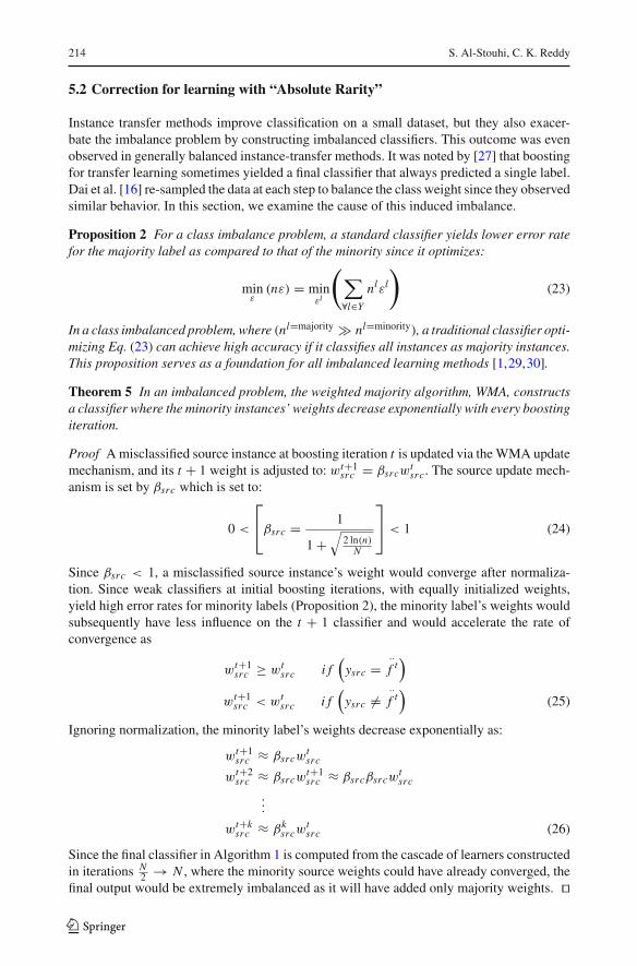
Instance transfer methods improve classification on a small dataset, but they also exacer-bate the imbalance problem by constructing imbalanced classifiers. This outcome was evenobserved in generally balanced instance-transfer methods. It was noted by [27] that boostingfor transfer learning sometimes yielded a final classifier that always predicted a single label.Dai et al. [16] re-sampled the data at each step to balance the class weight since they observedsimilar behavior. In this section, we examine the cause of this induced imbalance.

Proposition 2 For a class imbalance problem, a standard classifier yields lower error ratefor the majority label as compared to that of the minority since it optimizes:

minε

(nε) = minεl

(∑

∀l∈Y

nlεl

)

(23)

In a class imbalanced problem, where (nl=majority � nl=minority), a traditional classifier opti-mizing Eq. (23) can achieve high accuracy if it classifies all instances as majority instances.This proposition serves as a foundation for all imbalanced learning methods [1,29,30].

Theorem 5 In an imbalanced problem, the weighted majority algorithm, WMA, constructsa classifier where the minority instances’ weights decrease exponentially with every boostingiteration.

Proof Amisclassified source instance at boosting iteration t is updated via theWMA updatemechanism, and its t + 1 weight is adjusted to: wt+1

src = βsrcwtsrc. The source update mech-

anism is set by βsrc which is set to:

0 <

⎡

⎣βsrc = 1

1 +√

2 ln(n)N

⎤

⎦ < 1 (24)

Since βsrc < 1, a misclassified source instance’s weight would converge after normaliza-tion. Since weak classifiers at initial boosting iterations, with equally initialized weights,yield high error rates for minority labels (Proposition 2), the minority label’s weights wouldsubsequently have less influence on the t + 1 classifier and would accelerate the rate ofconvergence as

wt+1src ≥ wt

src i f(

ysrc =..

f t)

wt+1src < wt

src i f(

ysrc �=..

f t)

(25)

Ignoring normalization, the minority label’s weights decrease exponentially as:

wt+1src ≈ βsrcw

tsrc

wt+2src ≈ βsrcw

t+1src ≈ βsrcβsrcw

tsrc

...

wt+ksrc ≈ βk

srcwtsrc (26)

Since the final classifier in Algorithm 1 is computed from the cascade of learners constructedin iterations N

2 → N , where the minority source weights could have already converged, thefinal output would be extremely imbalanced as it will have added only majority weights. �

123


Conversely, updating the target instances via the AdaBoost update mechanism improvesthe performance on an imbalanced dataset particularly if the final classifier is computedusing only the N

2 → N boosting iterations. A misclassified target instance at boostingiteration t is updated via the AdaBoost update mechanism, and its t + 1 weight is adjustedto: wt+1

tar = βtarwttar . The target update for a misclassified instance’s weight is dependent on

βtar where

1 <

[βtar = 1 − εt

tar

εttar

]< ∞ (27)

Since βtar > 1, a misclassified target instance’s weight would increase after normalizationand the minority label’s weights would in turn have more influence on the t + 1 classifierand bias the classifier to improve learning on the minority as:

wt+1tar < wt

tar i f(

ytar =..

f t)

wt+1tar ≥ wt

tar i f(

ytar �=..

f t)

(28)

Since the final classifier is computed from the cascade of learners constructed in iterationsN2 → N , where the minority label’s instances have increased weights to compensate for thelack of its samples, the final output would be more balanced.

5.3 Label space optimization

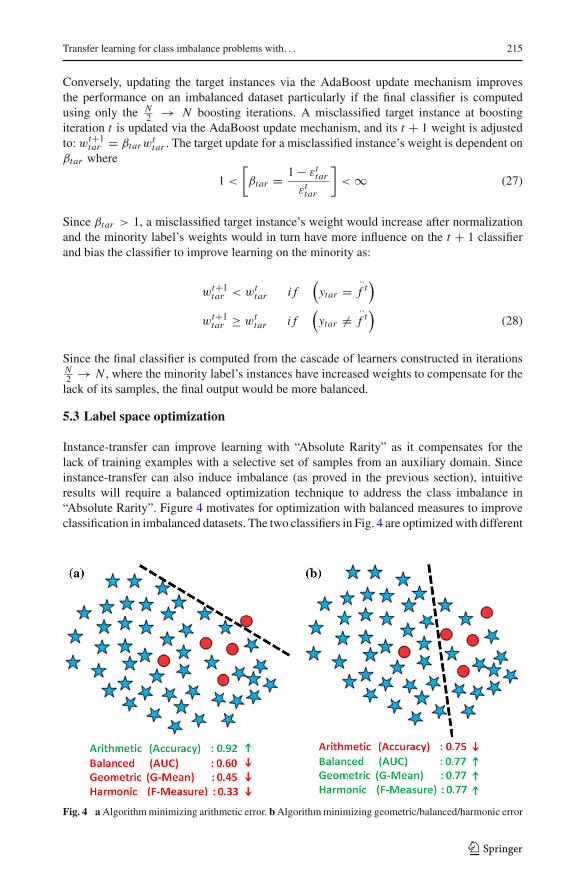
Instance-transfer can improve learning with “Absolute Rarity” as it compensates for thelack of training examples with a selective set of samples from an auxiliary domain. Sinceinstance-transfer can also induce imbalance (as proved in the previous section), intuitiveresults will require a balanced optimization technique to address the class imbalance in“Absolute Rarity”. Figure 4 motivates for optimization with balanced measures to improveclassification in imbalanced datasets. The two classifiers in Fig. 4 are optimizedwith different

Fig. 4 a Algorithmminimizing arithmetic error. b Algorithmminimizing geometric/balanced/harmonic error

123


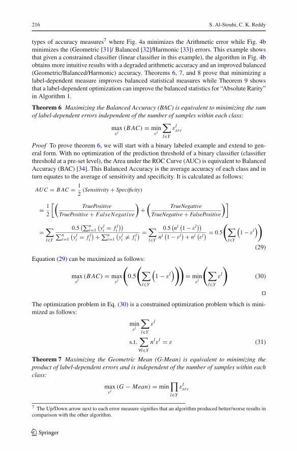
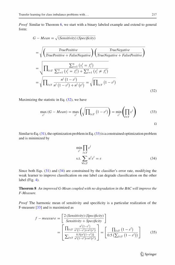
types of accuracy measures7 where Fig. 4a minimizes the Arithmetic error while Fig. 4bminimizes the (Geometric [31]/ Balanced [32]/Harmonic [33]) errors. This example showsthat given a constrained classifier (linear classifier in this example), the algorithm in Fig. 4bobtains more intuitive results with a degraded arithmetic accuracy and an improved balanced(Geometric/Balanced/Harmonic) accuracy. Theorems 6, 7, and 8 prove that minimizing alabel-dependent measure improves balanced statistical measures while Theorem 9 showsthat a label-dependent optimization can improve the balanced statistics for “Absolute Rarity”in Algorithm 1.

Theorem 6 Maximizing the Balanced Accuracy (BAC) is equivalent to minimizing the sumof label-dependent errors independent of the number of samples within each class:

maxεl

(B AC) = minεl

∑

l∈Y

εlsrc

Proof To prove theorem 6, we will start with a binary labeled example and extend to gen-eral form. With no optimization of the prediction threshold of a binary classifier (classifierthreshold at a pre-set level), the Area under the ROC Curve (AUC) is equivalent to BalancedAccuracy (BAC) [34]. This Balanced Accuracy is the average accuracy of each class and inturn equates to the average of sensitivity and specificity. It is calculated as follows:

AUC = B AC = 1

2(Sensitivity + Specificity)

= 1

2

[(TruePositive

TruePositive + FalseNegative

)+(

TrueNegative

TrueNegative + FalsePositive

)]

=∑

l∈Y

0.5(∑n

i=1

(yl

i = f li

))

∑ni=1

(yl

i = f li

)+∑ni=1

(yl

i �= f li

) =∑

l∈Y

0.5(nl(1 − εl

))

nl(1 − εl

)+ nl(εl) = 0.5

(∑

l∈Y

(1 − εl

))

(29)

Equation (29) can be maximized as follows:

maxεl

(B AC) = maxεl

(

0.5

(∑

l∈Y

(1 − εl

)))

= minεl

(∑

l∈Y

εl

)

(30)

�The optimization problem in Eq. (30) is a constrained optimization problem which is mini-mized as follows:

minεl

∑

l∈Y

εl

s.t.∑

∀l∈Y

nlεl = ε (31)

Theorem 7 Maximizing the Geometric Mean (G-Mean) is equivalent to minimizing theproduct of label-dependent errors and is independent of the number of samples within eachclass:

maxεl

(G − Mean) = min∏

l∈Y

εlsrc

7 The Up/Down arrow next to each error measure signifies that an algorithm produced better/worse results incomparison with the other algorithm.

123


Proof Similar to Theorem 6, we start with a binary labeled example and extend to generalform:

G − Mean = √(Sensitivity) (Specificity)

=√(

TruePositive

TruePositive + FalseNegative

)(TrueNegative

TrueNegative + FalsePositive

)

=√√√√∏

l∈Y

∑ni=1

(yl

i = f li

)

∑ni=1

(yl

i = f li

)+∑ni=1

(yl

i �= f li

)

=√∏

l∈Y

nl(1 − εl

)

nl(1 − εl

)+ nl(εl) =

√∏

l∈Y

(1 − εl

)

(32)

Maximizing the statistic in Eq. (32), we have

maxεl

(G − Mean) = maxεl

(√∏

l∈Y

(1 − εl

)) = minεl

(∏

l∈Y

εl

)

(33)

�

Similar toEq. (31), the optimization problem inEq. (33) is a constrainedoptimization problemand is minimized by

minεl

∏

l∈Y

εl

s.t.∑

∀l∈Y

nlεl = ε (34)

Since both Eqs. (31) and (34) are constrained by the classifier’s error rate, modifying theweak learner to improve classification on one label can degrade classification on the otherlabel (Fig. 4).

Theorem 8 An improved G-Mean coupled with no degradation in the BAC will improve theF-Measure.

Proof The harmonic mean of sensitivity and specificity is a particular realization of theF-measure [33] and is maximized as

f − measure =[2 (Sensitivity) (Specificity)

Sensitivity + Specificity

]

=⎡

⎢⎣

∏l∈Y

nl(1−εl

)

nl(1−εl)+nl(εl)∑

l∈Y0.5(nl(1−εl))

nl(1−εl)+nl(εl)

⎤

⎥⎦ =

[ ∏l∈Y

(1 − εl

)

0.5(∑

l∈Y

(1 − εl

))

]

(35)

123


Equation ( 35) can be optimized as

maxεl

( f − measure) = maxεl

[ ∏l∈Y

(1 − εl

)

0.5(∑

l∈Y

(1 − εl

))

]

= maxεl

[(G − Mean)2

B AC

]

= minεl

[(∏l∈Y εl

)

∑l∈Y εl

]

(36)

�Equation (36) proves a classifier that improves G-Mean (via balance) with no degradation inBAC (via Transfer) improves the F-measure.

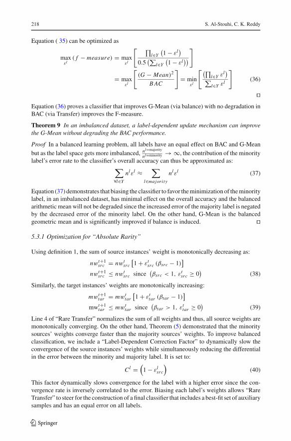
Theorem 9 In an imbalanced dataset, a label-dependent update mechanism can improvethe G-Mean without degrading the BAC performance.

Proof In a balanced learning problem, all labels have an equal effect on BAC and G-Mean

but as the label space gets more imbalanced, nl=majority

nl=minority → ∞, the contribution of the minoritylabel’s error rate to the classifier’s overall accuracy can thus be approximated as:

∑

∀l∈Y

nlεl ≈∑

l∈majori ty

nlεl (37)

Equation (37) demonstrates that biasing the classifier to favor theminimization of theminoritylabel, in an imbalanced dataset, has minimal effect on the overall accuracy and the balancedarithmetic mean will not be degraded since the increased error of the majority label is negatedby the decreased error of the minority label. On the other hand, G-Mean is the balancedgeometric mean and is significantly improved if balance is induced. �

5.3.1 Optimization for “Absolute Rarity”

Using definition 1, the sum of source instances’ weight is monotonically decreasing as:

nwt+1src = nwt

src

[1 + εt

src (βsrc − 1)]

nwt+1src ≤ nwt

src since(βsrc < 1, εt

src ≥ 0)

(38)

Similarly, the target instances’ weights are monotonically increasing:

mwt+1tar = mwt

tar

[1 + εt

tar (βtar − 1)]

mwt+1tar ≤ mwt

tar since(βtar > 1, εt

tar ≥ 0)

(39)

Line 4 of “Rare Transfer” normalizes the sum of all weights and thus, all source weights aremonotonically converging. On the other hand, Theorem (5) demonstrated that the minoritysources’ weights converge faster than the majority sources’ weights. To improve balancedclassification, we include a “Label-Dependent Correction Factor” to dynamically slow theconvergence of the source instances’ weights while simultaneously reducing the differentialin the error between the minority and majority label. It is set to:

Cl =(1 − εl

src

)(40)

This factor dynamically slows convergence for the label with a higher error since the con-vergence rate is inversely correlated to the error. Biasing each label’s weights allows “RareTransfer” to steer for the construction of a final classifier that includes a best-fit set of auxiliarysamples and has an equal error on all labels.

123


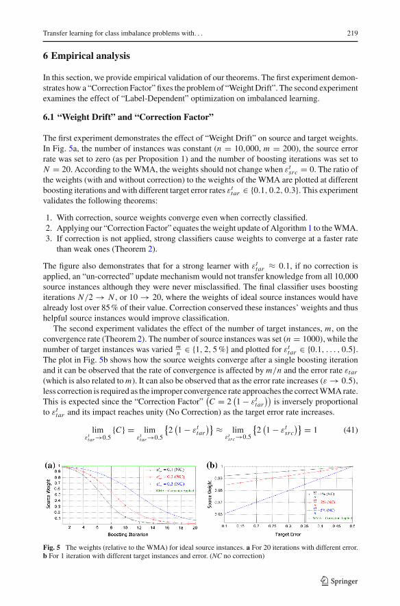
6 Empirical analysis

In this section, we provide empirical validation of our theorems. The first experiment demon-strates how a “Correction Factor” fixes the problemof “WeightDrift”. The second experimentexamines the effect of “Label-Dependent” optimization on imbalanced learning.

6.1 “Weight Drift” and “Correction Factor”

The first experiment demonstrates the effect of “Weight Drift” on source and target weights.In Fig. 5a, the number of instances was constant (n = 10,000, m = 200), the source errorrate was set to zero (as per Proposition 1) and the number of boosting iterations was set toN = 20. According to the WMA, the weights should not change when εt

src = 0. The ratio ofthe weights (with and without correction) to the weights of the WMA are plotted at differentboosting iterations and with different target error rates εt

tar ∈ {0.1, 0.2, 0.3}. This experimentvalidates the following theorems:

1. With correction, source weights converge even when correctly classified.2. Applying our “Correction Factor” equates theweight update of Algorithm 1 to theWMA.3. If correction is not applied, strong classifiers cause weights to converge at a faster rate

than weak ones (Theorem 2).

The figure also demonstrates that for a strong learner with εttar ≈ 0.1, if no correction is

applied, an “un-corrected” update mechanism would not transfer knowledge from all 10,000source instances although they were never misclassified. The final classifier uses boostingiterations N/2 → N , or 10 → 20, where the weights of ideal source instances would havealready lost over 85% of their value. Correction conserved these instances’ weights and thushelpful source instances would improve classification.

The second experiment validates the effect of the number of target instances, m, on theconvergence rate (Theorem 2). The number of source instances was set (n = 1000), while thenumber of target instances was varied m

n ∈ {1, 2, 5%} and plotted for εttar ∈ {0.1, . . . , 0.5}.

The plot in Fig. 5b shows how the source weights converge after a single boosting iterationand it can be observed that the rate of convergence is affected by m/n and the error rate εtar

(which is also related to m). It can also be observed that as the error rate increases (ε → 0.5),less correction is required as the improper convergence rate approaches the correctWMArate.This is expected since the “Correction Factor”

(C = 2

(1 − εt

tar

))is inversely proportional

to εttar and its impact reaches unity (No Correction) as the target error rate increases.

limεt

tar →0.5{C} = lim

εttar →0.5

{2(1 − εt

tar

)} ≈ limεt

src→0.5

{2(1 − εt

src

)} = 1 (41)

Fig. 5 The weights (relative to the WMA) for ideal source instances. a For 20 iterations with different error.b For 1 iteration with different target instances and error. (NC no correction)

123


0 5 10 15 20 25 30 35 40 45 500

0.10.20.30.40.50.60.70.80.91

Boosting Iteration

Acc

urac

y

Majority(No-Correction)Majority(Rare-Transfer)Minority(No-Correction)Minority(Rare-Transfer)

(a)

0 5 10 15 20 25 30 35 40 45 500

0.050.1

0.150.2

0.250.3

0.350.4

0.450.5

Boosting Iteration

BA

C

BAC(No-Correction)BAC(Rare-Transfer)

(b)

0 5 10 15 20 25 30 35 40 45 500

0.050.1

0.150.2

0.250.3

0.350.4

0.450.5

Boosting Iteration

G-M

ean

G-Mean(No-Correction)G-Mean(Rare-Transfer)

(c)

0 5 10 15 20 25 30 35 40 45 500

0.050.1

0.150.2

0.250.3

0.350.4

0.450.5

Boosting Iteration

F-M

easu

reF-Measure(No-Correction)F-Measure(Rare-Transfer)

(d)

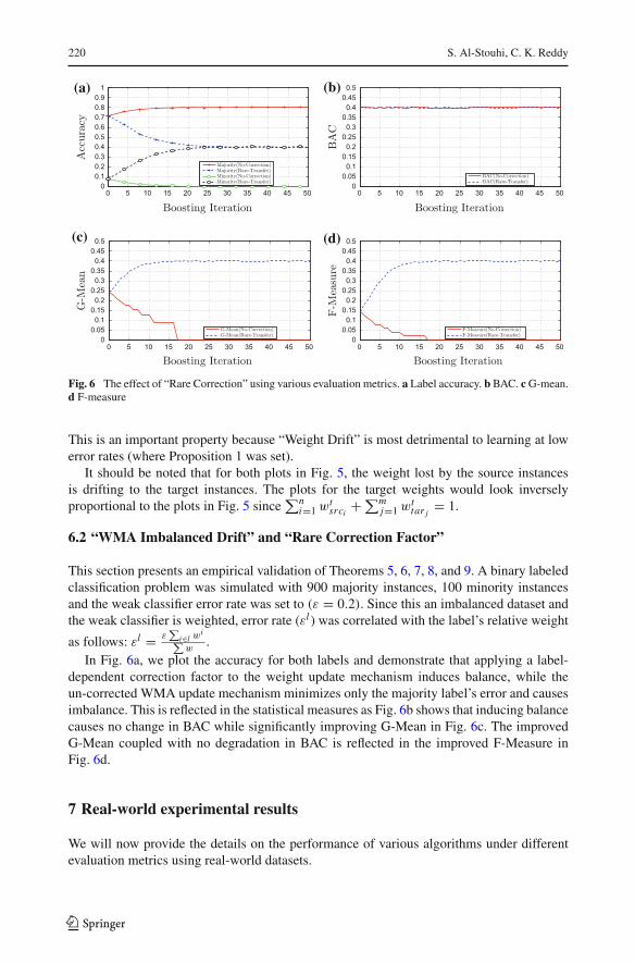
Fig. 6 The effect of “Rare Correction” using various evaluation metrics. a Label accuracy. b BAC. c G-mean.d F-measure

This is an important property because “Weight Drift” is most detrimental to learning at lowerror rates (where Proposition 1 was set).

It should be noted that for both plots in Fig. 5, the weight lost by the source instancesis drifting to the target instances. The plots for the target weights would look inverselyproportional to the plots in Fig. 5 since

∑ni=1 wt

srci+∑m

j=1 wttar j

= 1.

6.2 “WMA Imbalanced Drift” and “Rare Correction Factor”

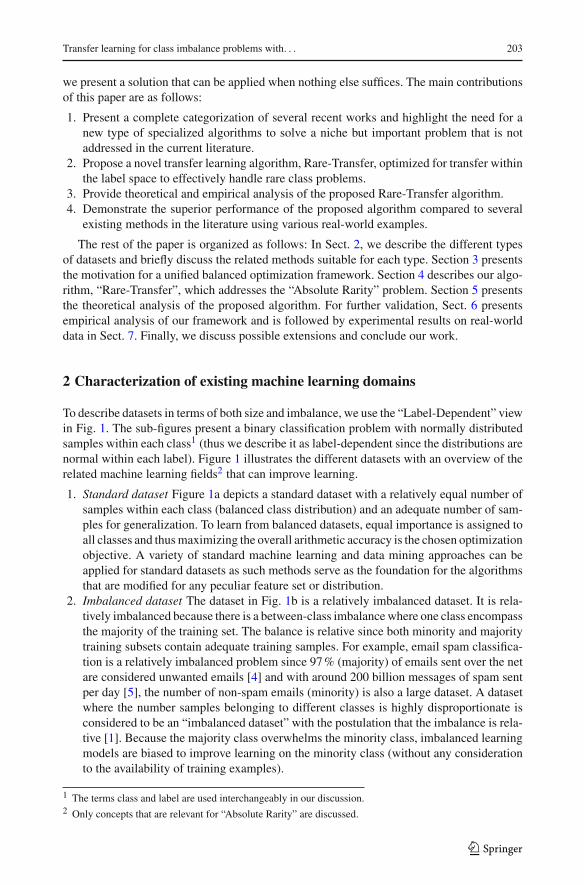
This section presents an empirical validation of Theorems 5, 6, 7, 8, and 9. A binary labeledclassification problem was simulated with 900 majority instances, 100 minority instancesand the weak classifier error rate was set to (ε = 0.2). Since this an imbalanced dataset andthe weak classifier is weighted, error rate (εl ) was correlated with the label’s relative weight

as follows: εl = ε∑

i∈l wi∑

w.

In Fig. 6a, we plot the accuracy for both labels and demonstrate that applying a label-dependent correction factor to the weight update mechanism induces balance, while theun-corrected WMA update mechanism minimizes only the majority label’s error and causesimbalance. This is reflected in the statistical measures as Fig. 6b shows that inducing balancecauses no change in BAC while significantly improving G-Mean in Fig. 6c. The improvedG-Mean coupled with no degradation in BAC is reflected in the improved F-Measure inFig. 6d.

7 Real-world experimental results

We will now provide the details on the performance of various algorithms under differentevaluation metrics using real-world datasets.

123


7.1 Dataset description

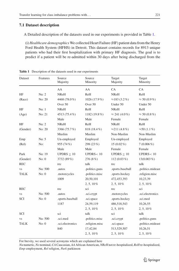
A Detailed description of the datasets used in our experiments is provided in Table 1.

(i)Healthcare demographicsWecollectedHeart Failure (HF) patient data from theHenryFord Health System (HFHS) in Detroit. This dataset contains records for 8913 uniquepatients who had their first hospitalization with primary HF diagnosis. The goal is topredict if a patient will be re-admitted within 30 days after being discharged from the

Table 1 Description of the datasets used in our experiments

Dataset Features Source Source Target TargetMajority Minority Majority Minority

AA AA CA CA

HF Nu: 2 NReH ReH NReH ReH

(Race) No: 20 4468 (78.0%) 1026 (17.9%) ≈183 (3.2%) ≈ 50 (0.9%)

Over 50 Over 50 Under 50 Under 50


(Age) No: 21 4513 (75.4%) 1182 (19.8%) ≈ 241 (4.0%) ≈ 50 (0.8%)

Male Male Female Female


(Gender) No: 20 3366 (75.7%) 818 (18.4%) ≈211 (4.8%) ≈50 (1.1%)

Muslim Muslim Non-Muslim Non-Muslim

Emp Nu: 5 Un-employed Employed Un-employed Employed

(Rel) No: 955 (74%) 298 (23%) 15 (0.02%) 7 (0.006%)

Male Male Female Female

Park Nu: 19 UPDRS ≥ 10 UPDRS< 10 UPDRS ≥ 10 UPDRS< 10

(Gender) No: 0 3732 (89%) 276 (8%) 112 (0.03%) 13(0.003%)

REC rec talk rec talk

vs Nu: 500 .autos .politics.guns .sports.baseball .politics.mideast

TALK No: 0 .motorcycles .politics.misc .sports.hockey .religion.misc

1009 20,50,101 472,453,393 10,23,39

2, 5, 10% 2, 5, 10% 2, 5, 10%

REC rec sci rec sci

vs Nu: 500 .autos .sci.crypt .motorcycles .sci.electronics

SCI No: 0 .sports.baseball .sci.space .sports.hockey .sci.med

1187 24,59,119 486,518,543 10,26,55

2, 5, 10% 2, 5, 10% 2, 5, 10%

SCI sci talk sci talk

vs Nu: 500 .sci.med .politics.misc .sci.crypt .politics.guns

TALK No: 0 .sci.electronics .religion.misc .sci.space .politics.mideast

840 17,42,84 513,529,507 10,26,51

2, 5, 10% 2, 5, 10% 2, 5, 10%

For brevity, we used several acronyms which are explained hereNu numeric,No nominal,CACaucasian,AAAfricanAmerican,NReH not re-hospitalized,ReH re-hospitalized,Emp employment, Rel religion, Park parkinson

123


hospital and to apply the model to rural hospitals or to demographics with less data[35]. Re-hospitalization for HF occurs in around one-in-five patients within 30 days ofdischarge and is disproportionately distributed across the US population with significantdisparities based on gender, age, ethnicity, geographic area, and socioeconomic sta-tus [36]. Other non-demographic features included length of hospital stay, ICU stay anddichotomous variables for whether a patient was diagnosed with diabetes, hypertension,peripheral vascular disease, transient ischemic attack, heart failure, chronic kidney dis-ease, coronary artery disease, hemodialysis treatment, cardiac catheterization, right heartcatheterization, coronary angiography, balloon pump, mechanical ventilation or generalintervention. The average results with 50 minority samples (patient was re-hospitalized)is reported.(ii) Employment dataset This dataset is a subset of the 1987 National Indonesia Con-traceptive Prevalence Survey [37]. We used the dataset [14] to predict if a non-Muslimwoman is employed based on her demographic and socio-economic characteristics. Inthe training set, only 22 of the 1275 were not Muslim and only 7 of them were employed.(iii) Parkinson dataset This dataset [38] is composed of a range of biomedical voicemeasurements from people with early-stage Parkinson’s disease. The goal is to predictif a female patient’s score on the Unified Parkinson’s Disease Rating Scale [39] is high(UPDRS≥ 10) or low (UPDRS<10). In the training set, only 125 of the 3732 participantswere female and only 13 of them had a low UPDRS score.(iv) Text dataset 20 Newsgroups8 is a popular text collection that is partitioned across20 groups with 3 cross-domain tasks and a two-level hierarchy as outlined in [40]. WeusedTermFrequencyInverseDocument Frequency (TF-IDF) [41] tomaintain around 500features and imbalanced the dataset to generate a high-dimensional, small and imbalanceddataset.

7.2 Experiment setup

AdaBoost [17] was used as the standard baseline algorithm for comparison. We appliedSMOTE [42], with 5 nearest neighbors (k = 5), before boosting to compare with an imbal-anced classification method (SMOTE-AdaBoost). TrAdaBoost [16] was used as the baselinetransfer learning algorithm. The non-transfer reference algorithms were trained with thetarget-only set and with the combined (target+source) set. Thirty boosting iterations wereexperimentally proven sufficient for training.

Base learner( ..

f)We did not use decision stumps as weak learners since most data belong

to the source and it was not possible to keep the target error below 0.5 (as mandated byAdaBoost) for more than a few iterations. A strong classifier, full classification tree withoutpruning, is applied with a top-down approach where the tree is trimmed at the first level toachieve εt

tar < 0.5.Cross validation Small datasets are prone to over-fit and terminate boosting and thus allalgorithms were restarted with a new cross validation fold when any algorithm terminatedbefore reaching 30 iterations. Random sub-sampling cross validation [43] was applied, andeach statistic was tabulated with the macro-average [44] of 30 runs. Plots with two imbalanceratios across a variable size of minority samples are also presented.

8 http://people.csail.mit.edu/jrennie/20Newsgroups/.

123

http://people.csail.mit.edu/jrennie/20Newsgroups/


7.3 Experimental results

This section presents the classification results for the different balanced learning measures.

7.3.1 BAC results

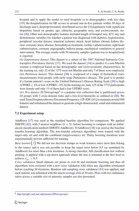
The BAC results presented in Table 2 show that Rare-Transfer improved the Balanced Accu-racy. The improved performance is consistent evenwhen the addition of auxiliary data seemedto degrade the performance as evident in the 20 Newsgroups dataset. This is proof that the“transfer learning” objective in our algorithm improved learning with only the best set of aux-iliary instances. Figure 7 demonstrates that the improved performance is consistent acrossdifferent datasets, imbalance ratios and absolute number of minority samples.

7.3.2 G-mean results

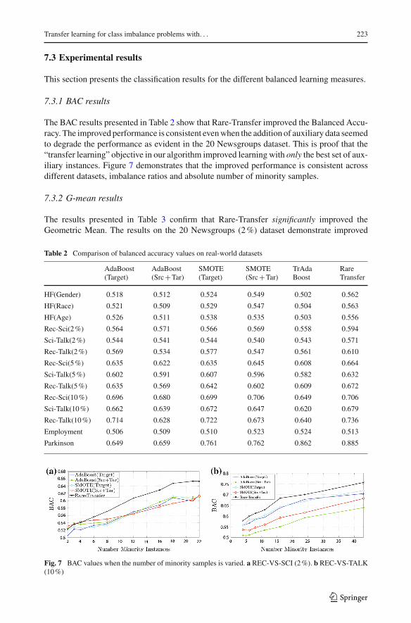
The results presented in Table 3 confirm that Rare-Transfer significantly improved theGeometric Mean. The results on the 20 Newsgroups (2%) dataset demonstrate improved

Table 2 Comparison of balanced accuracy values on real-world datasets

AdaBoost(Target)

AdaBoost(Src+Tar)

SMOTE(Target)

SMOTE(Src+Tar)

TrAdaBoost

RareTransfer

HF(Gender) 0.518 0.512 0.524 0.549 0.502 0.562

HF(Race) 0.521 0.509 0.529 0.547 0.504 0.563

HF(Age) 0.526 0.511 0.538 0.535 0.503 0.556

Rec-Sci(2%) 0.564 0.571 0.566 0.569 0.558 0.594

Sci-Talk(2%) 0.544 0.541 0.544 0.540 0.543 0.571

Rec-Talk(2%) 0.569 0.534 0.577 0.547 0.561 0.610

Rec-Sci(5%) 0.635 0.622 0.635 0.645 0.608 0.664

Sci-Talk(5%) 0.602 0.591 0.607 0.596 0.582 0.632

Rec-Talk(5%) 0.635 0.569 0.642 0.602 0.609 0.672

Rec-Sci(10%) 0.696 0.680 0.699 0.706 0.649 0.706

Sci-Talk(10%) 0.662 0.639 0.672 0.647 0.620 0.679

Rec-Talk(10%) 0.714 0.628 0.722 0.673 0.640 0.736

Employment 0.506 0.509 0.510 0.523 0.524 0.513

Parkinson 0.649 0.659 0.761 0.762 0.862 0.885

Fig. 7 BAC values when the number of minority samples is varied. a REC-VS-SCI (2%). b REC-VS-TALK(10%)

123


Table 3 Comparison of G-mean values on real-world datasets

AdaBoost(Target)

AdaBoost(Src+Tar)

SMOTE(Target)

SMOTE(Src+Tar)

TrAdaBoost

RareTransfer

HF(Gender) 0.336 0.212 0.444 0.459 0.117 0.518

HF(Race) 0.366 0.178 0.467 0.478 0.145 0.540

HF(Age) 0.346 0.141 0.447 0.357 0.164 0.478

Rec-Sci(2%) 0.324 0.362 0.338 0.379 0.384 0.430

Sci-Talk(2%) 0.270 0.271 0.277 0.292 0.339 0.380

Rec-Talk(2%) 0.343 0.221 0.378 0.293 0.387 0.460

Rec-Sci(5%) 0.500 0.492 0.501 0.561 0.512 0.592

Sci-Talk(5%) 0.433 0.423 0.446 0.464 0.471 0.541

Rec-Talk(5%) 0.502 0.340 0.516 0.450 0.491 0.591

Rec-Sci(10%) 0.615 0.605 0.623 0.671 0.581 0.674

Sci-Talk(10%) 0.563 0.531 0.584 0.575 0.531 0.637

Rec-Talk(10%) 0.647 0.483 0.661 0.597 0.569 0.702

Employment 0.422 0.452 0.467 0.483 0.331 0.378

Parkinson 0.518 0.570 0.715 0.741 0.841 0.874

Fig. 8 G-mean values when the number of minority samples is varied. a REC-VS-SCI (2%). b REC-VS-TALK (10%)

performance with severe label imbalance and an extremely high features/samples ratio (10minority samples, ≈500 majority samples, 500 features). Figure 8 shows that Rare-Transferconsistently yield superior results even after the non-transfer algorithms construct represen-tative hypotheses with more training samples.

7.3.3 F-measure results

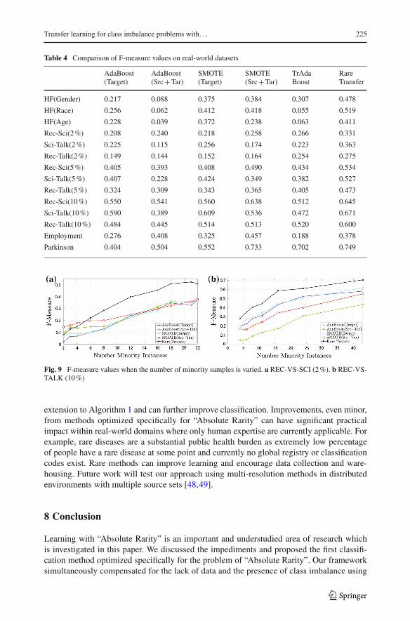
The F-Measure results are presented in Table 4 and demonstrate that Rare-Transfer constructsa more balanced classifier. The improvements are consistent at different imbalance ratios andsample sizes as shown in Fig. 9. The figures also demonstrate that the classification modelscan construct classifiers that are more balanced when the overall size of the training setincreases.

7.4 Discussion and possible extensions

Traditional imbalanced modifications including SMOTEBoost [45], over or under sam-pling [46] followed by transfer [47] or cost-sensitive learning [25] are a straight-forward

123


Table 4 Comparison of F-measure values on real-world datasets

AdaBoost(Target)

AdaBoost(Src+Tar)

SMOTE(Target)

SMOTE(Src+Tar)

TrAdaBoost

RareTransfer

HF(Gender) 0.217 0.088 0.375 0.384 0.307 0.478

HF(Race) 0.256 0.062 0.412 0.418 0.055 0.519

HF(Age) 0.228 0.039 0.372 0.238 0.063 0.411

Rec-Sci(2%) 0.208 0.240 0.218 0.258 0.266 0.331

Sci-Talk(2%) 0.225 0.115 0.256 0.174 0.223 0.363

Rec-Talk(2%) 0.149 0.144 0.152 0.164 0.254 0.275

Rec-Sci(5%) 0.405 0.393 0.408 0.490 0.434 0.534

Sci-Talk(5%) 0.407 0.228 0.424 0.349 0.382 0.527

Rec-Talk(5%) 0.324 0.309 0.343 0.365 0.405 0.473

Rec-Sci(10%) 0.550 0.541 0.560 0.638 0.512 0.645

Sci-Talk(10%) 0.590 0.389 0.609 0.536 0.472 0.671

Rec-Talk(10%) 0.484 0.445 0.514 0.513 0.520 0.600

Employment 0.276 0.408 0.325 0.457 0.188 0.378

Parkinson 0.404 0.504 0.552 0.733 0.702 0.749

Fig. 9 F-measure values when the number of minority samples is varied. a REC-VS-SCI (2%). b REC-VS-TALK (10%)

extension to Algorithm 1 and can further improve classification. Improvements, even minor,from methods optimized specifically for “Absolute Rarity” can have significant practicalimpact within real-world domains where only human expertise are currently applicable. Forexample, rare diseases are a substantial public health burden as extremely low percentageof people have a rare disease at some point and currently no global registry or classificationcodes exist. Rare methods can improve learning and encourage data collection and ware-housing. Future work will test our approach using multi-resolution methods in distributedenvironments with multiple source sets [48,49].

8 Conclusion

Learning with “Absolute Rarity” is an important and understudied area of research whichis investigated in this paper. We discussed the impediments and proposed the first classifi-cation method optimized specifically for the problem of “Absolute Rarity”. Our frameworksimultaneously compensated for the lack of data and the presence of class imbalance using

123


a transfer learning paradigm with a balanced statistics objective. We theoretically analyzedand empirically verified our work and demonstrated its effectiveness with several real-worlddomains. We proposed possible extensions and motivated for more research for a problemwith significant social and financial impact.

Acknowledgments This workwas supported in part by theNational Cancer Institute of theNational Institutesof Health under Award Number R21CA175974 and the US National Science Foundation grants IIS-1231742,IIS-1242304, and IIS-1527827. The content is solely the responsibility of the authors and does not necessarilyrepresent the official views of the NIH and NSF.

References

1. He H, Garcia E (2009) Learning from imbalanced data. IEEE Trans Knowl Data Eng 21(9):1263–12842. Pan SJ, Yang Q (2010) A survey on transfer learning. IEEE Trans Knowl Data Eng 22(10):1345–13593. Li Y, Vinzamuri B, Reddy CK (2015) Constrained elastic net based knowledge transfer for healthcare

information exchange. Data Min Knowl Discov 29(4):1094–11124. Waters D (2009) Spam overwhelms e-mail messages. BBCNews. http://news.bbc.co.uk/2/hi/technology/

7988579.stm5. Halliday J (2011) Email spam level bounces back after record low. The Guardian; Retrieved 2011-01-116. KearnsMJ, Vazirani UV (1994) An introduction to computational learning theory. MIT Press, Cambridge7. Mitchell T (1997) Machine learning. McGraw-Hill, New York8. Weiss GM (2004) Mining with rarity: a unifying framework. SIGKDD Explor Newsl 6(1):7–199. He J (2010) Rare category analysis. Ph.D. thesis; Carnegie Mellon University

10. Banko M, Brill E (2001) Scaling to very very large corpora for natural language disambiguation. In:Proceedings of the 39th annual meeting on association for computational linguistics. Association forComputational Linguistics, pp 26–33

11. Weiss GM, Provost F (2003) Learning when training data are costly: the effect of class distribution ontree induction. J Artif Intell Res 19(1):315–354

12. Japkowicz N, Stephen S (2002) The class imbalance problem: a systematic study. Intell Data Anal6(5):429–449

13. BradleyAP (1997)The use of the area under the roc curve in the evaluation ofmachine learning algorithms.Pattern Recognit 30(7):1145–1159

14. Frank A, Asuncion A (2010) UCI machine learning repository. http://archive.ics.uci.edu/ml15. Davis J, Goadrich M (2006) The relationship between precision-recall and roc curves. In: Proceedings of

the 23rd international conference on machine learning. ACM, pp 233–24016. DaiW, Yang Q, Xue GR, Yu Y (2007a) Boosting for transfer learning. In: Proceedings of the international

conference on machine learning, pp 193–20017. Freund Y, Schapire RE (1995) A decision-theoretic generalization of on-line learning and an application

to boosting. In: Proceedings of the second European conference on computational learning theory, pp23–37

18. Littlestone N, Warmuth MK (1989) The weighted majority algorithm. In: Proceedings of the 30th annualsymposium on foundations of computer science, pp 256–261

19. Yao Y, Doretto G (2010) Boosting for transfer learning with multiple sources. In: Proceedings of the IEEEconference on computer vision and pattern recognition (CVPR), pp 1855–1862

20. Al-Stouhi S, Reddy CK, Lanfear DE (2012) Label space transfer learning. In: IEEE 24th internationalconference on tools with artificial intelligence, ICTAI 2012, Athens, Greece, November 7–9, 2012, pp727–734

21. Vieriu RL, Rajagopal A, Subramanian R, Lanz O, Ricci E, Sebe N et al (2012) Boosting-based transferlearning for multi-view head-pose classification from surveillance videos. In: Proceedings of the 20thEuropean signal processing conference (EUSIPCO), pp 649–653

22. Luo W, Li X, Li W, Hu W (2011) Robust visual tracking via transfer learning. In: ICIP, pp 485–48823. Eaton E, Des Jardins M (2009) Set-based boosting for instance-level transfer. In: Proceedings of the 2009

IEEE international conference on data mining workshops, pp 422 –42824. Venkatesan A, Krishnan N, Panchanathan S (2010) Cost–sensitive boosting for concept drift. In: Pro-

ceedings of the 2010 international workshop on handling concept drift in adaptive information systems,pp 41–47

123

http://news.bbc.co.uk/2/hi/technology/7988579.stm

http://news.bbc.co.uk/2/hi/technology/7988579.stm

http://archive.ics.uci.edu/ml


25. Sun Y, Kamel MS, Wong AK, Wang Y (2007) Cost-sensitive boosting for classification of imbalanceddata. Pattern Recognit 40(12):3358–3378

26. Pardoe D, Stone P (2010) Boosting for regression transfer. In: Proceedings of the 27th internationalconference on machine learning, pp 863–870

27. Eaton E (2009) Selective knowledge transfer for machine learning. Ph.D. thesis. University of MarylandBaltimore County

28. Al-Stouhi S,ReddyCK(2011)Adaptive boosting for transfer learning using dynamic updates. In:Machinelearning and knowledge discovery in databases. Springer, Berlin, pp 60–75

29. Provost F (2000) Machine learning from imbalanced data sets 101. In: Proceedings of the Americanassociation for artificial intelligence workshop, pp 1–3

30. Ertekin S, Huang J, Bottou L, Giles L (2007) Learning on the border: active learning in imbalanceddata classification. In: Proceedings of the sixteenth ACM conference on conference on information andknowledge management, pp 127–136

31. Kubat M, Holte RC, Matwin S (1998) Machine learning for the detection of oil spills in satellite radarimages. Mach Learn 30(2–3):195–215

32. Guyon I, Aliferis CF, Cooper GF, Elisseeff A, Pellet JP, Spirtes P et al (2008) Design and analysis of thecausation and prediction challenge. J Mach Learn Res Proc Track 3:1–33

33. Rijsbergen CJV (1979) Information retrieval, 2nd edn. Butterworth-Heinemann, Newton,ISBN:0408709294

34. Brodersen K, Ong CS, StephanK, Buhmann J (2010) The balanced accuracy and its posterior distribution.In: Pattern recognition (ICPR), 2010 20th international conference on, pp 3121–3124

35. Vinzamuri B, Reddy CK (2013) Cox regression with correlation based regularization for electronic healthrecords. In: Data mining (ICDM), 2013 IEEE 13th international conference on. IEEE, pp 757–766

36. Clancy C, Munier W, Crosson K, Moy E, Ho K, FreemanW et al (2011) 2010 National healthcare qualityand disparities reports. Tech. Rep, Agency for Healthcare Research and Quality (AHRQ)

37. Gertler P, Molyneaux J (1994) How economic development and family planning programs combined toreduce indonesian fertility. Demography 31(1):33–63. doi:10.2307/2061907

38. LittleMA,McSharry PE,Hunter EJ, Spielman J, RamigLO (2009) Suitability of dysphoniameasurementsfor telemonitoring of parkinson’s disease. IEEE Trans Biomed Eng 56(4):1015–1022

39. Fahn S, Elton R, Committee UD et al (1987) Unified parkinson’s disease rating scale. Recent Dev Parkin-son’s Dis 2:153–163

40. Dai W, Xue GR, Yang Q, Yu Y (2007b) Co-clustering based classification for out-of-domain documents.In: Proceedings of the 13th ACM SIGKDD international conference on Knowledge discovery and datamining, pp 210–219

41. AizawaA (2003)An information-theoretic perspective of tf–idfmeasures. Inf ProcessManag 39(1):45–6542. Chawla N, Bowyer K, Hall L, Kegelmeyer W (2002) Smote: synthetic minority over-sampling technique.

J Artif Intell Res 16:321–35743. Kohavi R, et al (1995) A study of cross-validation and bootstrap for accuracy estimation and model selec-

tion. In: International joint conference on artificial intelligence; vol. 14. Lawrence Erlbaum AssociatesLtd, pp 1137–1145

44. Yang Y (1999) An evaluation of statistical approaches to text categorization. Inf Retr 1(1):69–9045. Chawla NV, Lazarevic A, Hall LO, Bowyer KW (2003) Smoteboost: improving prediction of the minority

class in boosting. In: Proceedings of the principles of knowledge discovery in databases, PKDD-2003,pp 107–119

46. Batista G, Prati R, Monard M (2004) A study of the behavior of several methods for balancing machinelearning training data. ACM SIGKDD Explor Newsl 6(1):20–29

47. Wang Y, Xiao J (2011) Transfer ensemble model for customer churn prediction with imbalanced classdistribution. In: Information technology, computer engineering and management sciences (ICM), 2011international conference on. vol. 3. IEEE, pp 177–181

48. Palit I, Reddy CK (2012) Scalable and parallel boosting with mapreduce. IEEE Trans Knowl Data Eng24(10):1904–1916

49. Reddy CK, Park JH (2011) Multi-resolution boosting for classification and regression problems. KnowlInf Syst 29(2):435–456

123

http://dx.doi.org/10.2307/2061907


Samir Al-Stouhi is a research engineering member of the Automo-bile Technology Research (ATR) group at Honda. He received hisPh.D. from the Electrical and Computer Engineering Department atWayne State University. His primary research interests are in the areaof machine learning with applications to localization via sensor fusion,transfer learning, multi-task learning and imbalanced learning.

Chandan K. Reddy is an Associate Professor in the Department ofComputer Science at Wayne State University. He received his Ph.D.from Cornell University and MS from Michigan State University. Hisprimary research interests are in the areas of data mining and machinelearning with applications to healthcare, bioinformatics, and social net-work analysis. His research is funded by the NSF, NIH, DOT, SusanG. Komen for the Cure Foundation. He has published over 50 peer-reviewed articles in leading conferences and journals. He received theBest Application Paper Award at the ACM SIGKDD conference in2010 and was a finalist of the INFORMS Franz Edelman Award Com-petition in 2011. He is a senior member of the IEEE and a life memberof the ACM.

123

Documents

Transfer learning for class imbalance problems with ...dmkd.cs.vt.edu/papers/KAIS16.pdfTransfer learning for class imbalance problems with inadequate data ... training and the generalization