Embed Size (px)
Citation preview
Transfer Maps for Beams with Space Charge
Transfer Maps for Beams with Space Charge
Bela ErdelyiDepartment of Physics, Northern Illinois University,and Physics Division, Argonne National Laboratory
Informal Workshop, Bloomington, March 15-17, 2010
Bela ErdelyiDepartment of Physics, Northern Illinois University,and Physics Division, Argonne National Laboratory
Informal Workshop, Bloomington, March 15-17, 2010
March 15-17, 2010 Space Charge Maps 2
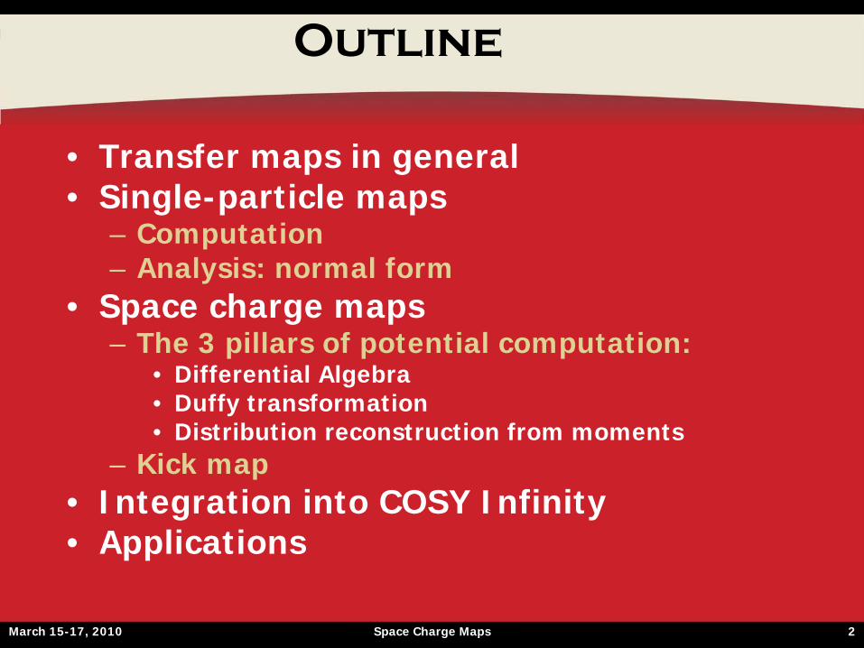
Outline
• Transfer maps in general• Single-particle maps
– Computation– Analysis: normal form
• Space charge maps– The 3 pillars of potential computation:
• Differential Algebra• Duffy transformation• Distribution reconstruction from moments
– Kick map• Integration into COSY Infinity• Applications
March 15-17, 2010 Space Charge Maps 3
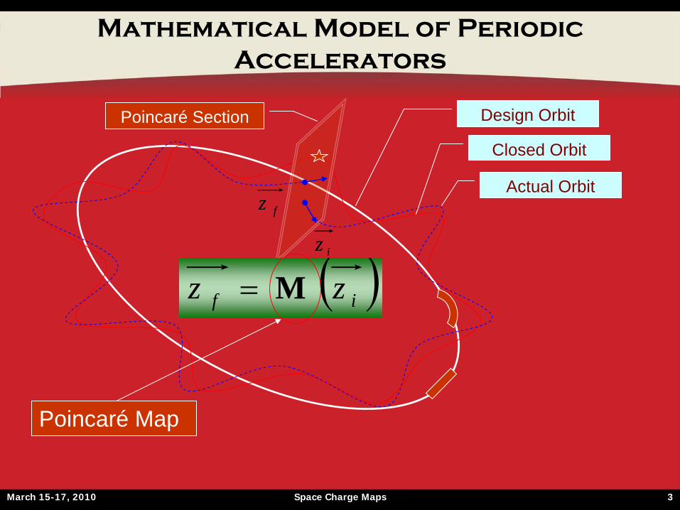
Design Orbit
Closed Orbit
Actual Orbit
Poincaré Section
iz
fz
if zz M
Poincaré Map
Mathematical Model of Periodic Accelerators
March 15-17, 2010 Space Charge Maps 4
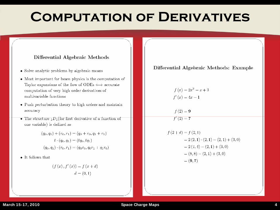
Computation of Derivatives
March 15-17, 2010 Space Charge Maps 5
Advanced Applications
• (1 D1 ,∂) can be generalized into (n Dv , ∂1 , …, ∂v ) for computation of derivatives up to order n of functions in v variables
• It can be generalized to vector functions (transfer maps)
• Composition of maps: given two vector functions with known derivatives up to order n, what are the derivatives of their composition? If M(0) = 0, then
[ N ◦
M ]n = [ N ]n ◦
[ M ]n
• Can be used to compute inverses [M-1]n
March 15-17, 2010 Space Charge Maps 6
Applications in Beam Physics
March 15-17, 2010 Space Charge Maps 7
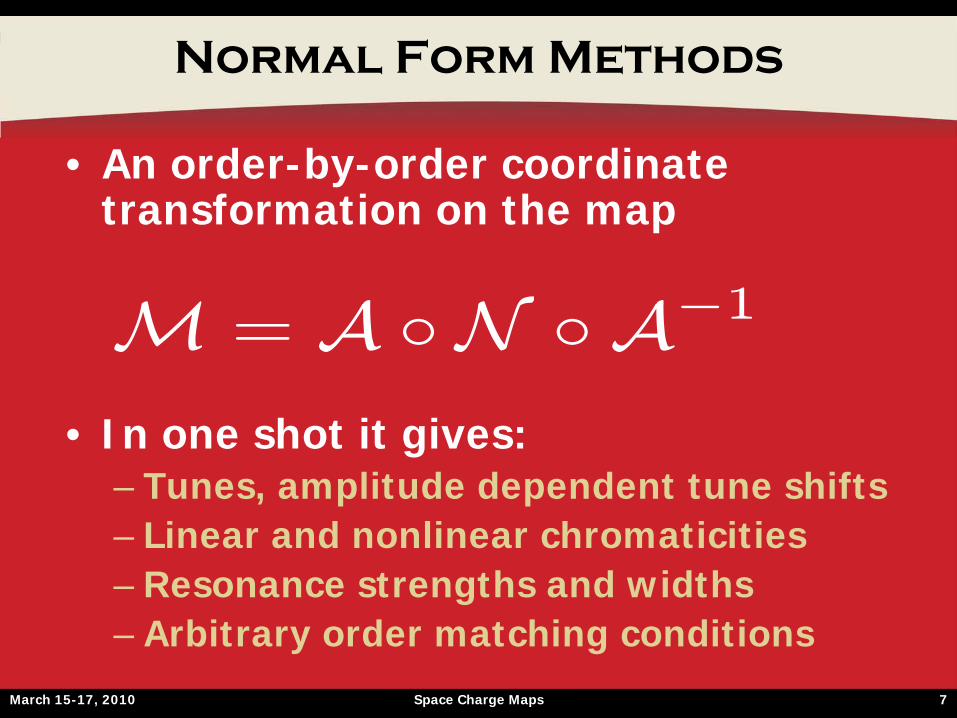
Normal Form Methods
• An order-by-order coordinate transformation on the map
• In one shot it gives:– Tunes, amplitude dependent tune shifts– Linear and nonlinear chromaticities– Resonance strengths and widths– Arbitrary order matching conditions
M = A ◦N ◦A−1
March 15-17, 2010 Space Charge Maps 8
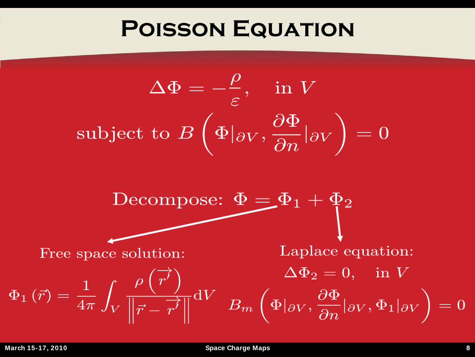
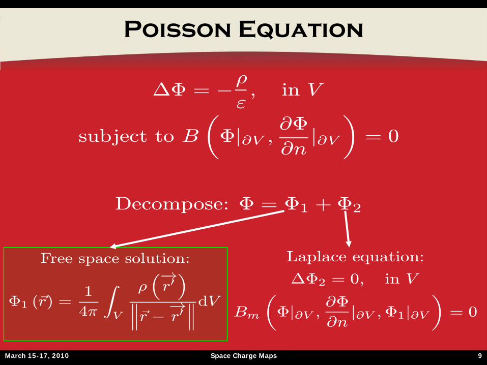
Poisson Equation
∆Φ = −ρ
ε, in V
subject to B
µΦ|∂V ,
∂Φ
∂n|∂V¶= 0
Decompose: Φ = Φ1 + Φ2
Free space solution:
Φ1 (~r) =1
4π
ZV
ρ³−→r0´
°°°~r −−→r0 °°°dVLaplace equation:
∆Φ2 = 0, in V
Bm
µΦ|∂V ,
∂Φ
∂n|∂V ,Φ1|∂V
¶= 0
March 15-17, 2010 Space Charge Maps 9
Poisson Equation
∆Φ = −ρ
ε, in V
subject to B
µΦ|∂V ,
∂Φ
∂n|∂V¶= 0
Decompose: Φ = Φ1 + Φ2
Free space solution:
Φ1 (~r) =1
4π
ZV
ρ³−→r0´
°°°~r −−→r0 °°°dVLaplace equation:
∆Φ2 = 0, in V
Bm
µΦ|∂V ,
∂Φ
∂n|∂V ,Φ1|∂V
¶= 0
March 15-17, 2010 Space Charge Maps 10
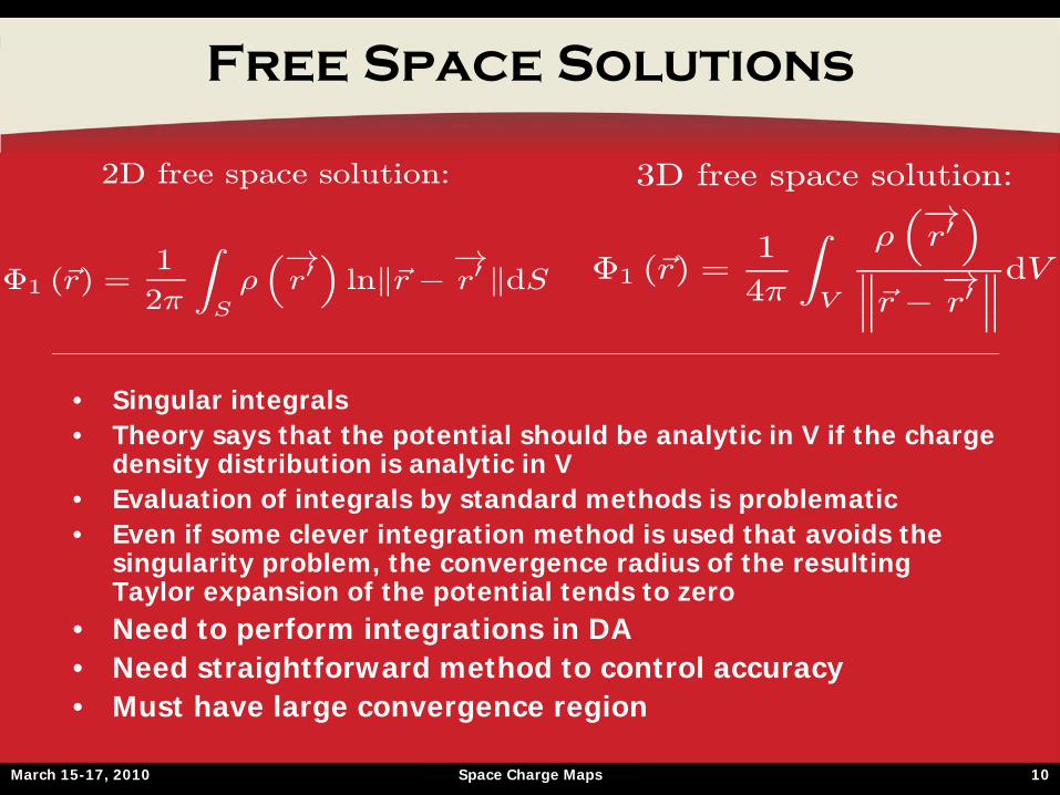
Free Space Solutions
3D free space solution:
Φ1 (~r) =1
4π
ZV
ρ³−→r0´
°°°~r −−→r0 °°°dV2D free space solution:
Φ1 (~r) =1
2π
ZS
ρ³−→r0´lnk~r −
−→r0 kdS
• Singular integrals• Theory says that the potential should be analytic in V if the charge
density distribution is analytic in V• Evaluation of integrals by standard methods is problematic• Even if some clever integration method is used that avoids the
singularity problem, the convergence radius of the resulting Taylor expansion of the potential tends to zero
• Need to perform integrations in DA• Need straightforward method to control accuracy• Must have large convergence region
March 15-17, 2010 Space Charge Maps 11
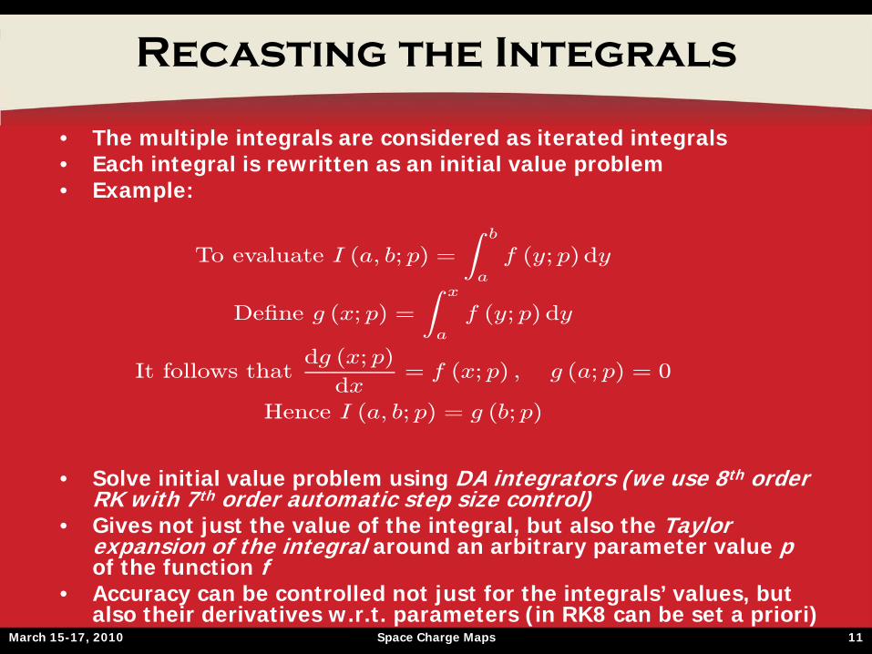
Recasting the Integrals
• The multiple integrals are considered as iterated integrals• Each integral is rewritten as an initial value problem• Example:
• Solve initial value problem using DA integrators (we use 8th order RK with 7th order automatic step size control)
• Gives not just the value of the integral, but also the Taylor expansion of the integral around an arbitrary parameter value p of the function f
• Accuracy can be controlled not just for the integrals’ values, but also their derivatives w.r.t. parameters (in RK8 can be set a priori)
To evaluate I (a, b; p) =
Z b
a
f (y; p) dy
Define g (x; p) =
Z x
a
f (y; p) dy
It follows thatdg (x; p)
dx= f (x; p) , g (a; p) = 0
Hence I (a, b; p) = g (b; p)
March 15-17, 2010 Space Charge Maps 12
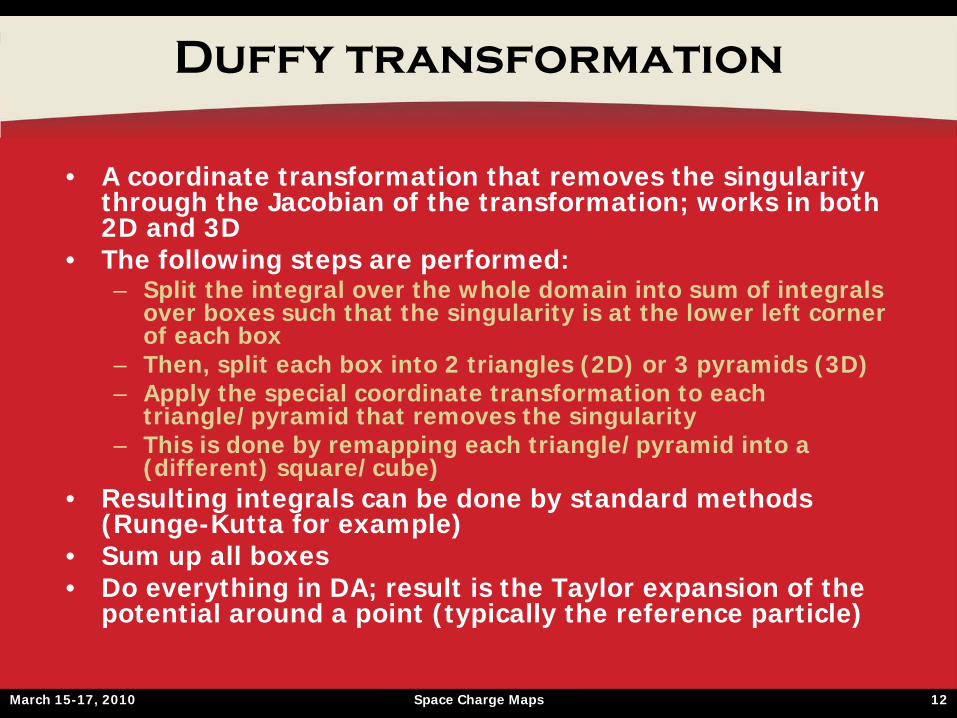
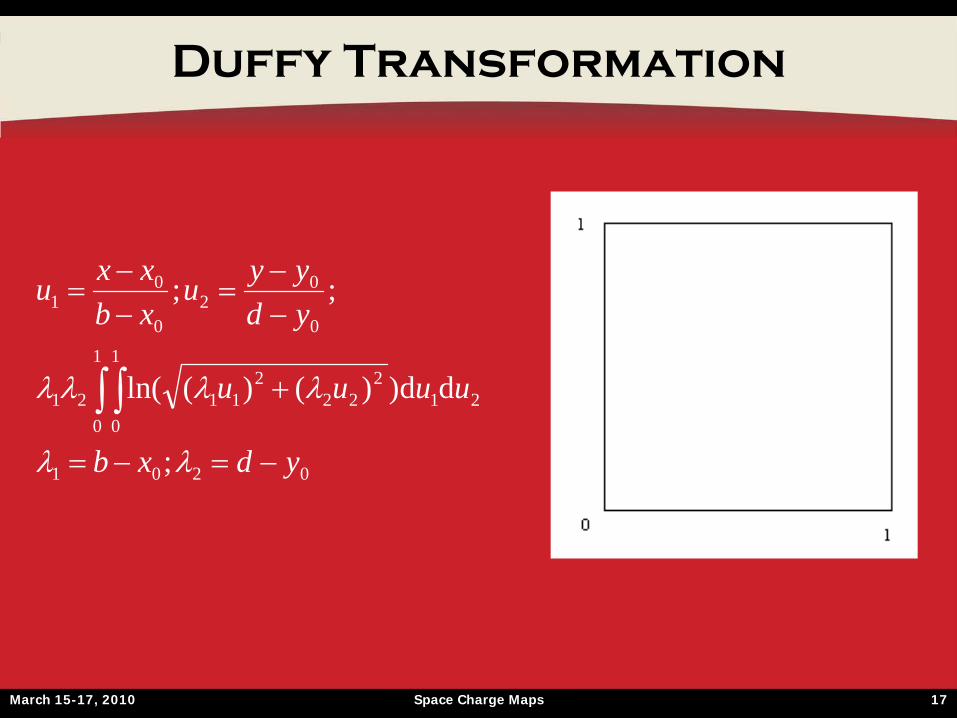
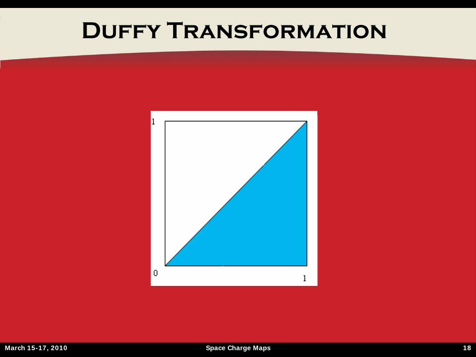
Duffy transformation
• A coordinate transformation that removes the singularity through the Jacobian of the transformation; works in both 2D and 3D
• The following steps are performed:– Split the integral over the whole domain into sum of integrals
over boxes such that the singularity is at the lower left corner of each box
– Then, split each box into 2 triangles (2D) or 3 pyramids (3D)– Apply the special coordinate transformation to each
triangle/pyramid that removes the singularity– This is done by remapping each triangle/pyramid into a
(different) square/cube)• Resulting integrals can be done by standard methods
(Runge-Kutta for example)• Sum up all boxes• Do everything in DA; result is the Taylor expansion of the
potential around a point (typically the reference particle)
March 15-17, 2010 Space Charge Maps 13
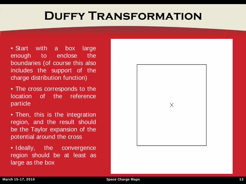
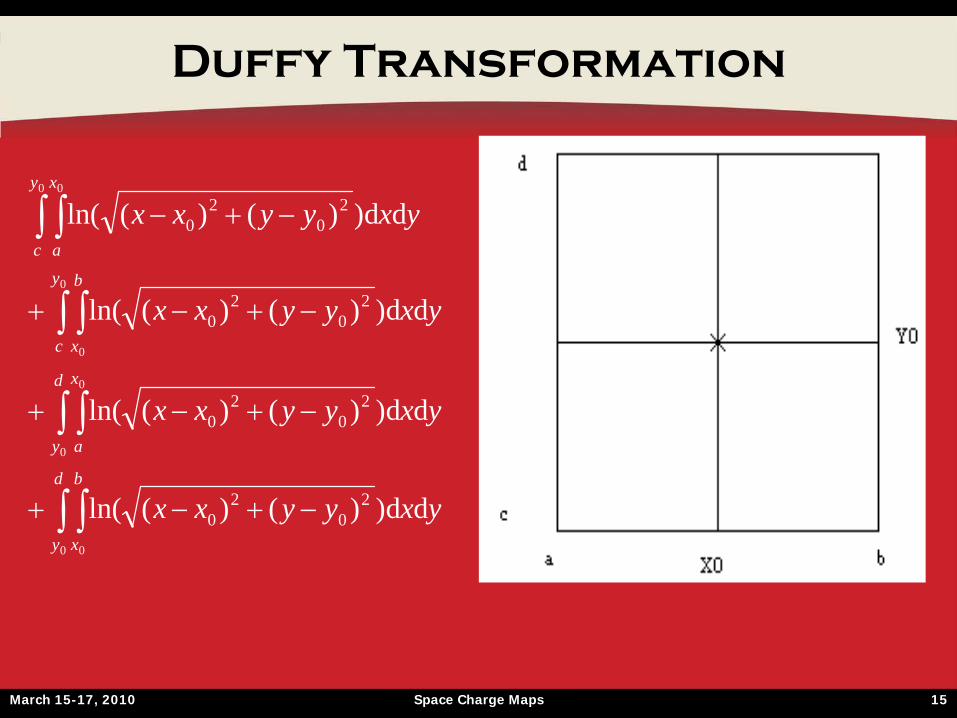
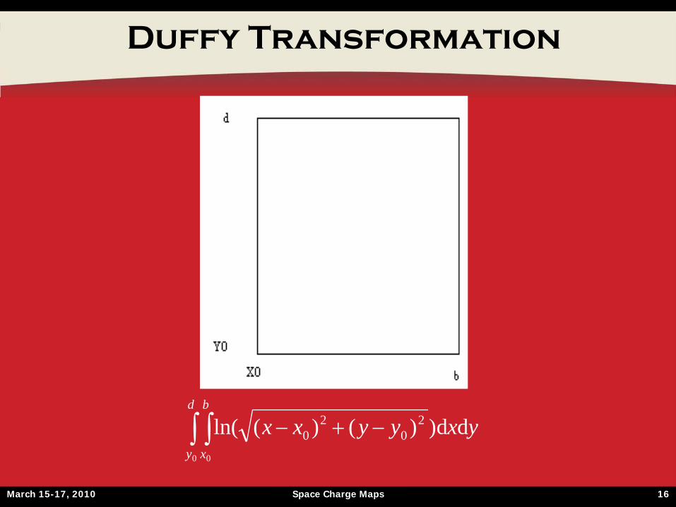
Duffy Transformation
• Start with a box large enough to enclose the boundaries (of course this also includes the support of the charge distribution function)
• The cross corresponds to the location of the reference particle
• Then, this is the integration region, and the result should be the Taylor expansion of the potential around the cross
• Ideally, the convergence region should be at least as large as the box
March 15-17, 2010 Space Charge Maps 14
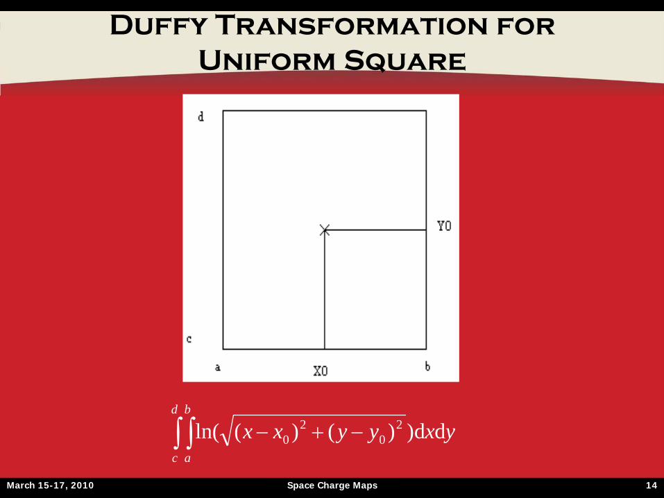
Duffy Transformation for Uniform Square
d
c
b
a
yxyyxx dd))()(ln( 20
20
March 15-17, 2010 Space Charge Maps 15
d
y
b
x
d
y
x
a
y
c
b
x
y
c
x
a
yxyyxx
yxyyxx
yxyyxx
yxyyxx
0 0
0
0
0
0
0 0
dd))()(ln(
dd))()(ln(
dd))()(ln(
dd))()(ln(
20
20
20
20
20
20
20
20
Duffy Transformation
March 15-17, 2010 Space Charge Maps 16
d
y
b
x
yxyyxx0 0
dd))()(ln( 20
20
Duffy Transformation
March 15-17, 2010 Space Charge Maps 17
0201
1
0
1
021
222
21121
0
02
0
01
;
dd))()(ln(
;;
ydxb
uuuu
ydyyu
xbxxu
Duffy Transformation
March 15-17, 2010 Space Charge Maps 18
Duffy Transformation
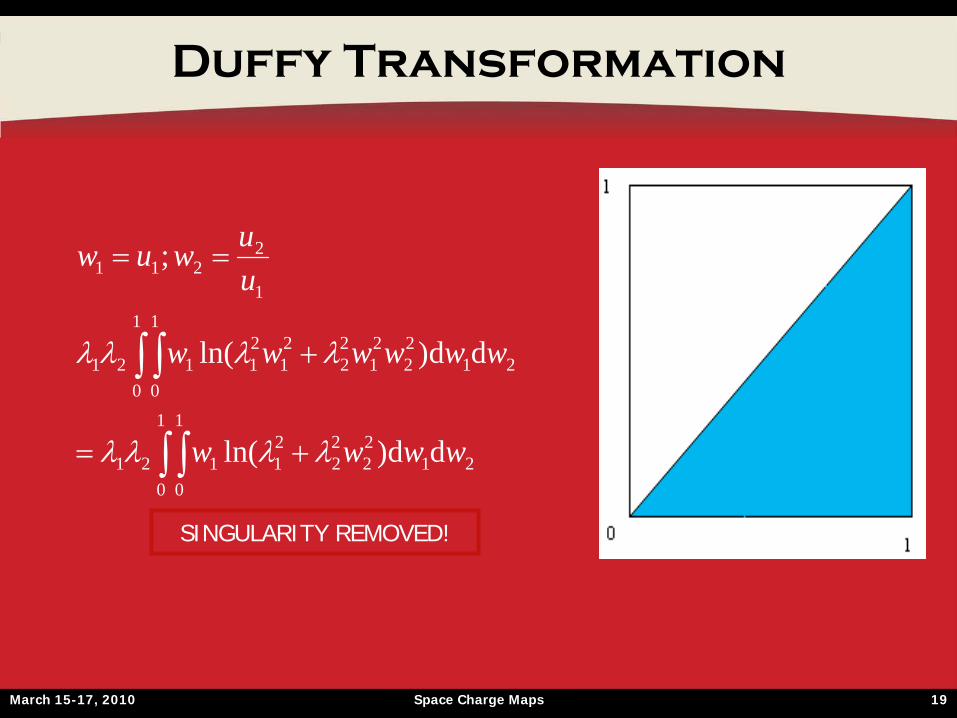
March 15-17, 2010 Space Charge Maps 19
Duffy Transformation
2122
22
1
0
1
0
21121
2122
21
22
1
0
1
0
21
21121
1
2211
dd)ln(
dd)ln(
;
wwww
wwwwww
uuwuw
SINGULARITY REMOVED!
March 15-17, 2010 Space Charge Maps 20
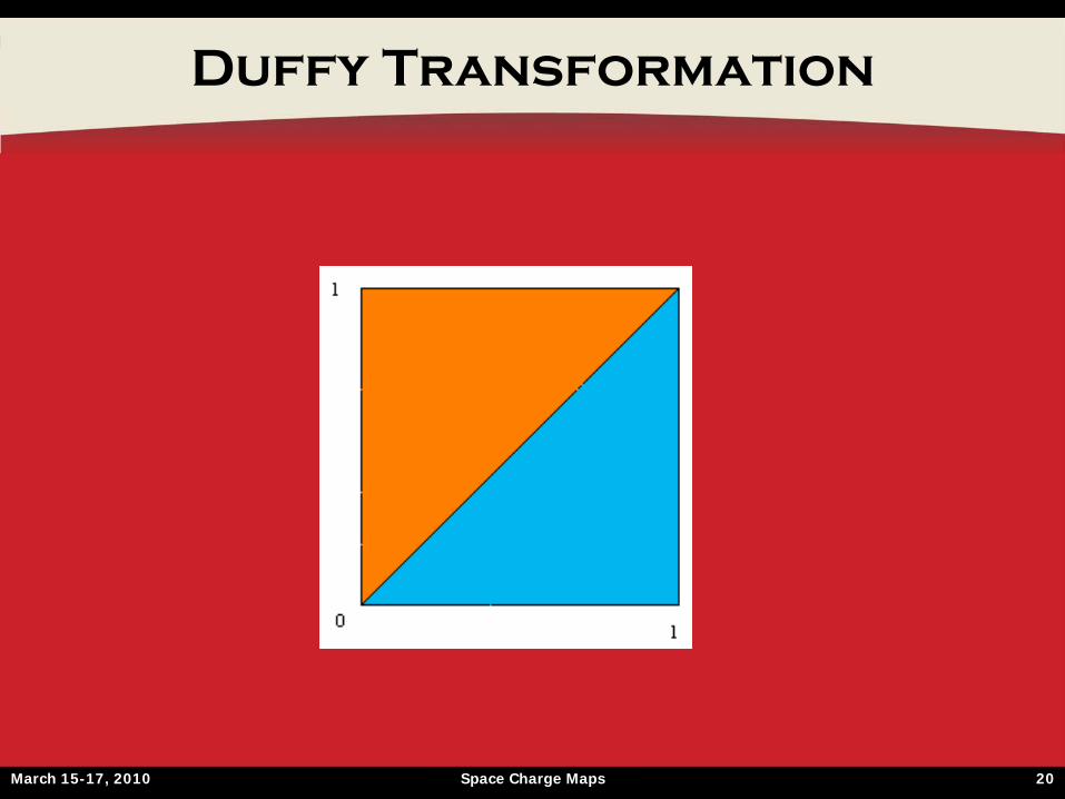
Duffy Transformation
March 15-17, 2010 Space Charge Maps 21
Duffy Transformation
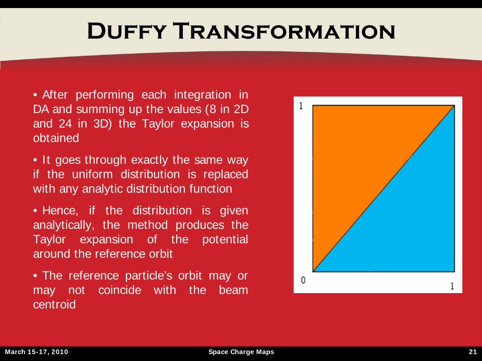
• After performing each integration in DA and summing up the values (8 in 2D and 24 in 3D) the Taylor expansion is obtained
• It goes through exactly the same way if the uniform distribution is replaced with any analytic distribution function
• Hence, if the distribution is given analytically, the method produces the Taylor expansion of the potential around the reference orbit
• The reference particle’s orbit may or may not coincide with the beam centroid
March 15-17, 2010 Space Charge Maps 22
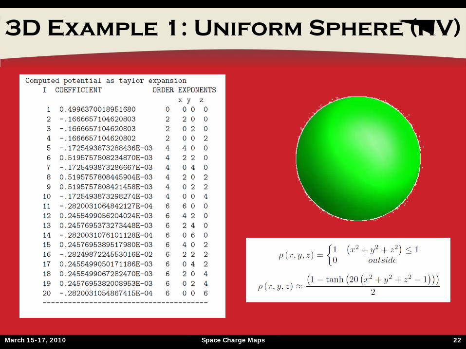
3D Example 1: Uniform Sphere (KV)
March 15-17, 2010 Space Charge Maps 23
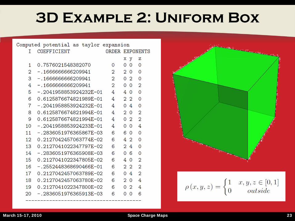
3D Example 2: Uniform Box
March 15-17, 2010 Space Charge Maps 24
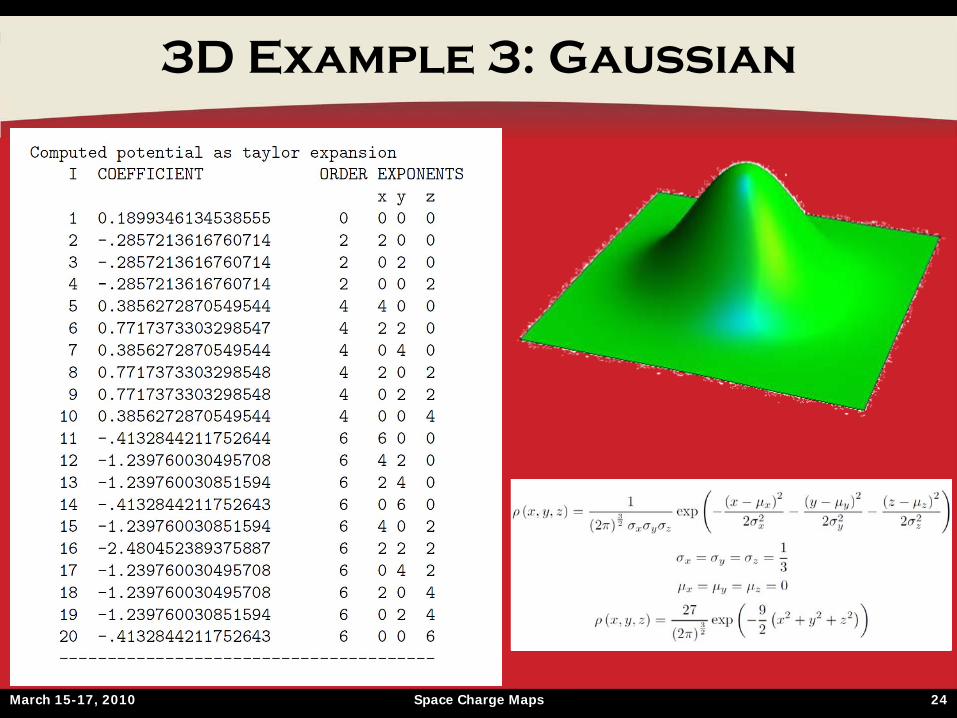
3D Example 3: Gaussian
March 15-17, 2010 Space Charge Maps 25
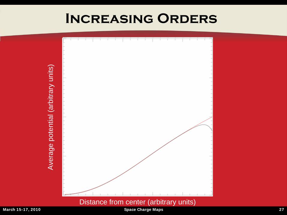
Convergence Region
• It can be shown that the region of convergence of the multiple Taylor series of the potential is a box with sides equal to the closest boundaries in each spatial direction
• Therefore, it is advantageous to pick the computational box symmetric w.r.t. the expansion point
• According to theory, by rearranging the Taylor series into a sequence of homogeneous polynomials, the convergence region becomes a star- shaped region that cannot be smaller than the original convergence region
March 15-17, 2010 Space Charge Maps 26
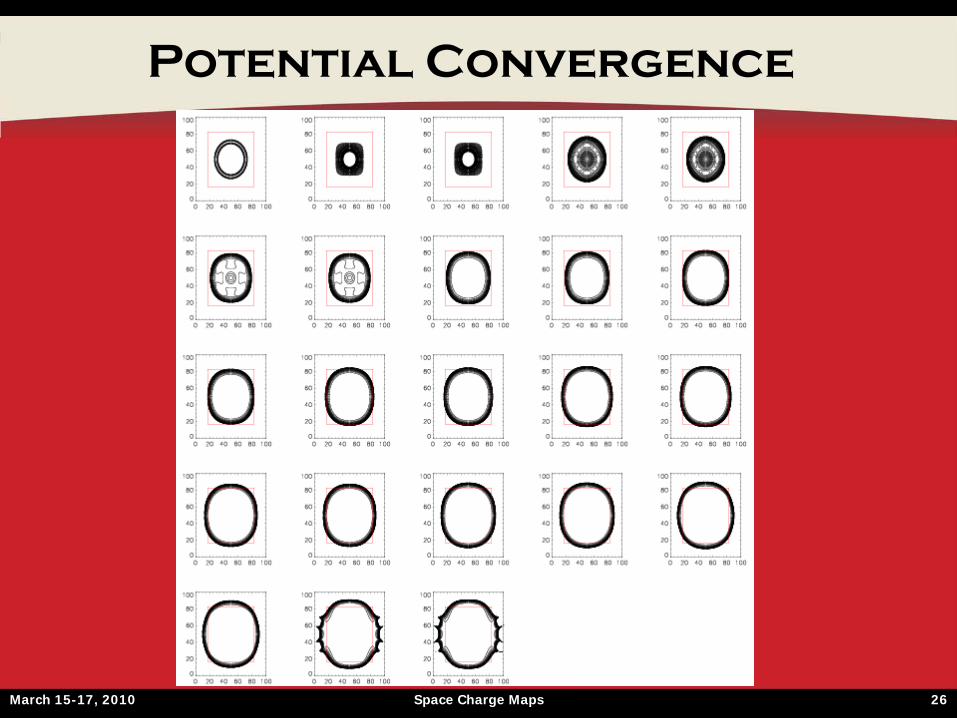
Potential Convergence
March 15-17, 2010 Space Charge Maps 27
Increasing Orders
Distance from center (arbitrary units)
Ave
rage
pot
entia
l (ar
bitra
ry u
nits
)
March 15-17, 2010 Space Charge Maps 28
Moments of the distribution
• If the distribution is not known analytically, can it be reconstructed from something?
• Yes, from the moments of the distribution
• Theorem: smooth distribution functions with compact support (and some with non-compact support, such as the Gaussian) are uniquely determined by their moments
March 15-17, 2010 Space Charge Maps 29
Moments of the distribution
• What can be said in the case of a finite set of common moments?
• The distributions sharing a finite set of common moments will resemble each other
• What is the convergence like in the limit of large number of same moments?
• Interestingly, the tail probabilities converge faster!
March 15-17, 2010 Space Charge Maps 30
Convergence of the Moment Method
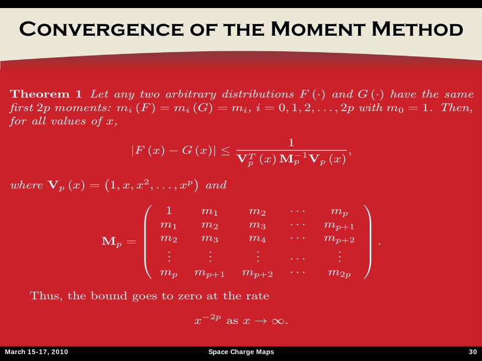
Theorem 1 Let any two arbitrary distributions F (·) and G (·) have the samefirst 2p moments: mi (F ) = mi (G) = mi, i = 0, 1, 2, . . . , 2p with m0 = 1. Then,for all values of x,
|F (x)−G (x)| ≤ 1
VTp (x)M
−1p Vp (x)
,
where Vp (x) =¡1, x, x2, . . . , xp
¢and
Mp =
⎛⎜⎜⎜⎜⎜⎝1 m1 m2 · · · mp
m1 m2 m3 · · · mp+1
m2 m3 m4 · · · mp+2
......
... · · ·...
mp mp+1 mp+2 · · · m2p
⎞⎟⎟⎟⎟⎟⎠ .
Thus, the bound goes to zero at the rate
x−2p as x→∞.
March 15-17, 2010 Space Charge Maps 31
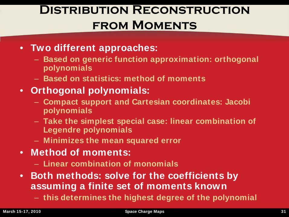
Distribution Reconstruction from Moments
• Two different approaches:– Based on generic function approximation: orthogonal
polynomials– Based on statistics: method of moments
• Orthogonal polynomials:– Compact support and Cartesian coordinates: Jacobi
polynomials– Take the simplest special case: linear combination of
Legendre polynomials– Minimizes the mean squared error
• Method of moments:– Linear combination of monomials
• Both methods: solve for the coefficients by assuming a finite set of moments known – this determines the highest degree of the polynomial
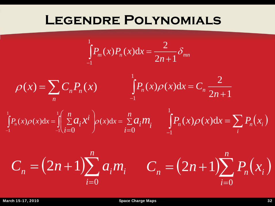
March 15-17, 2010 Space Charge Maps 32
1
1 122d)()(
nCxxxP nn
nnn xPCx )()(
1
1 122d)()( mnnm n
xxPxP
Legendre Polynomials
1
1
1
1 0d)(
0d)()( i
n
iixxin
iixxxP maxan
n
iiin manC
012
1
1
d)()(i
inn xPxxxP
n
iinn xPnC
012
March 15-17, 2010 Space Charge Maps 33
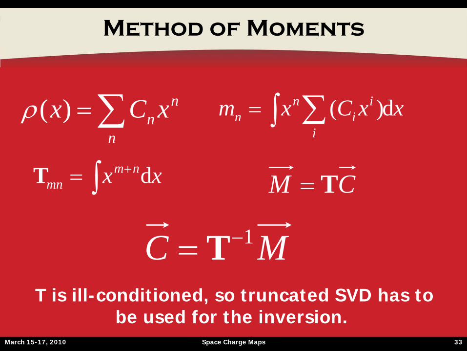
Method of Moments
CM T
n
nnxCx)( xxCxm
i
ii
nn d)(
MC 1 TT is ill-conditioned, so truncated SVD has to
be used for the inversion.
xx nmmn dT
March 15-17, 2010 Space Charge Maps 34
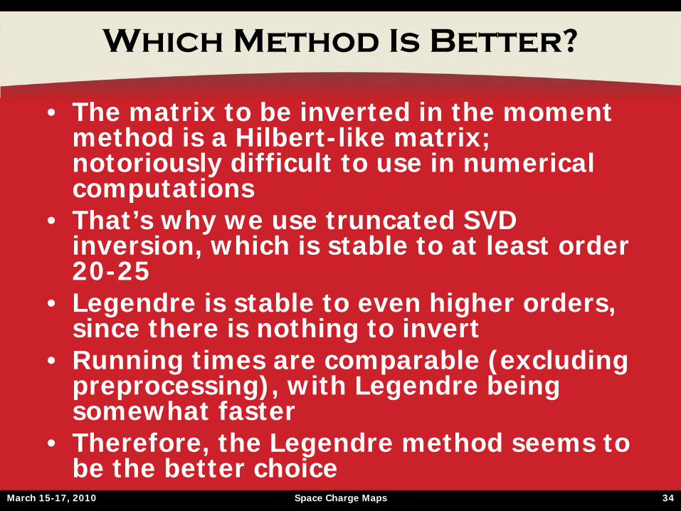
Which Method Is Better?
• The matrix to be inverted in the moment method is a Hilbert-like matrix; notoriously difficult to use in numerical computations
• That’s why we use truncated SVD inversion, which is stable to at least order 20-25
• Legendre is stable to even higher orders, since there is nothing to invert
• Running times are comparable (excluding preprocessing), with Legendre being somewhat faster
• Therefore, the Legendre method seems to be the better choice
March 15-17, 2010 Space Charge Maps 35
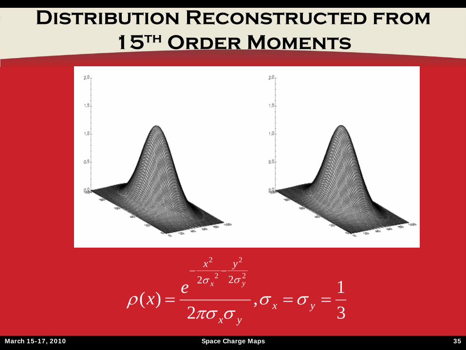
31,
2)(
2
2
2
2
22
yxyx
yx
yxex
Distribution Reconstructed from 15th
Order Moments
March 15-17, 2010 Space Charge Maps 36
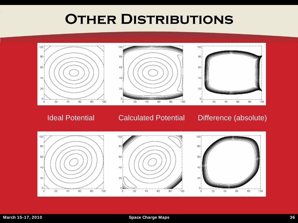
Other Distributions
Ideal Potential Calculated Potential Difference (absolute)
March 15-17, 2010 Space Charge Maps 37
Sample moments vs. True Moments
• In practice, not only we don’t know the analytical distribution, but also we don’t know the true moments
• All we have is a finite number of particles from which we can compute a finite set of sample moments
• Replace the true moments with sample moments everywhere
• Does anything change significantly?
March 15-17, 2010 Space Charge Maps 38
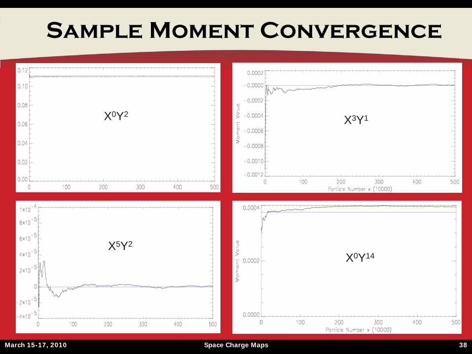
Sample Moment Convergence
X0Y2
X5Y2
X0Y14
X3Y1
March 15-17, 2010 Space Charge Maps 39
Reconstruction Methods Revisited
• If sample moments are used instead of true moments, is it still true that Legendre is better?
• Interestingly, no!• The reason is that the difference between
the true and sample moments can be thought of as an error in the right hand sides of two systems of linear equation that determine the distribution coefficients in the two methods
• It is well-known that the relative error in the solution of the linear systems will depend on the condition number of the system matrix
March 15-17, 2010 Space Charge Maps 40
Reconstruction with Sample moments
~cL = A~m ~cM = T−1 ~mkδ~cLkk~cLk
≤ κ (A)kδ~mkk~mk
kδ~cMkk~cMk
≤ κ (T)kδ~mkk~mk
and due to the truncated SVD inversion of T: κ (T) < κ (A)
• Of course, the same SVD truncation could be performed on A too, but this extra effort renders the Legendre method somewhat slower than the moment method
• Hence, the moment method in general is less sensitive to errors in the (sample) moments and it is faster
• Therefore, for realistic problems the moment method is preferred in general
• Side note: in some cases Legendre might still be preferable (for example multimodal and/or oscillatory distributions)
March 15-17, 2010 Space Charge Maps 41
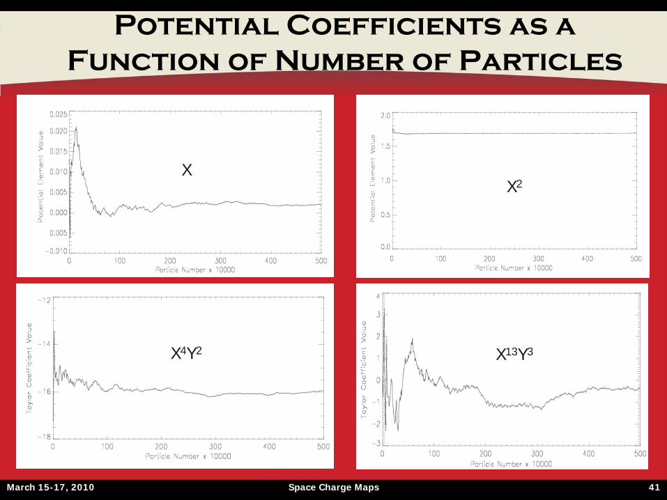
Potential Coefficients as a Function of Number of Particles
X2X
X4Y2 X13Y3
March 15-17, 2010 Space Charge Maps 42
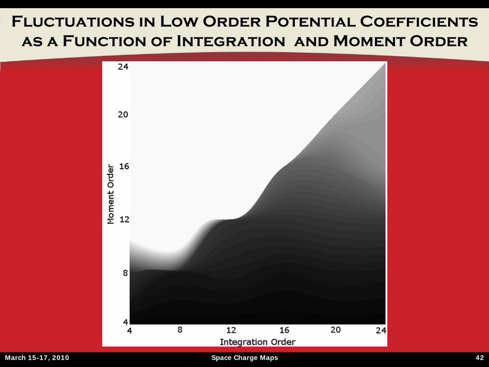
Fluctuations in Low Order Potential Coefficients as a Function of Integration and Moment Order
March 15-17, 2010 Space Charge Maps 43
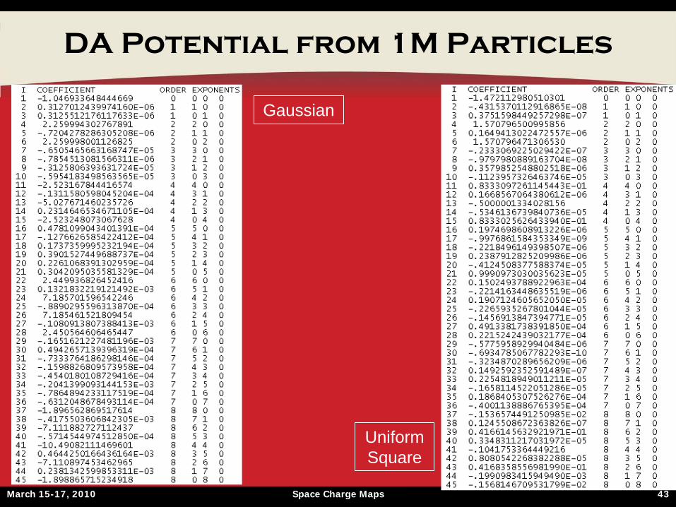
DA Potential from 1M Particles
Gaussian
Uniform Square
March 15-17, 2010 Space Charge Maps 44
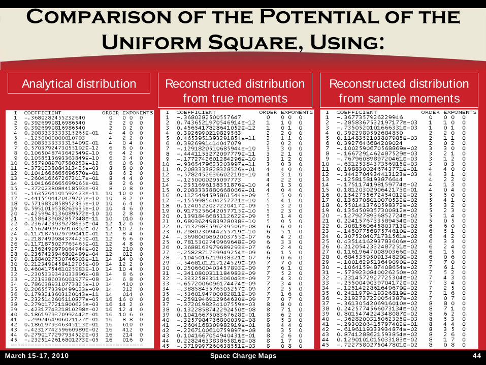
Comparison of the Potential of the Uniform Square, Using:
Analytical distribution Reconstructed distribution from true moments
Reconstructed distribution from sample moments
March 15-17, 2010 Space Charge Maps 45
Kick Map
• Once the Taylor expansion of the potential is computed, take derivative to obtain the fields in the beam frame
• Note that this is an elementary operation in DA, so there are no interpolation errors
• Lorentz boost to lab frame• Substitute into the equations of motion• Apply splitting and composition
techniques• Obtain space charge kick map from DA
integration of the EOM in the same way as in the single-particle case
March 15-17, 2010 Space Charge Maps 46
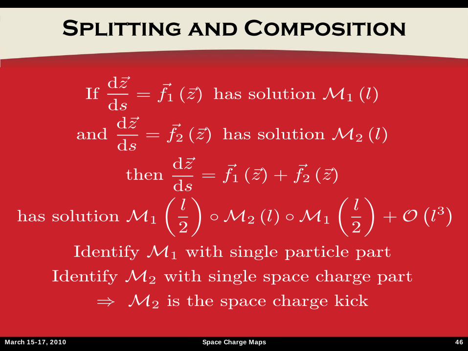
Splitting and Composition
Ifd~z
ds= ~f1 (~z) has solutionM1 (l)
andd~z
ds= ~f2 (~z) has solutionM2 (l)
thend~z
ds= ~f1 (~z) + ~f2 (~z)
has solutionM1
µl
2
¶◦M2 (l) ◦M1
µl
2
¶+O
¡l3¢
IdentifyM1 with single particle part
IdentifyM2 with single space charge part
⇒ M2 is the space charge kick
March 15-17, 2010 Space Charge Maps 47
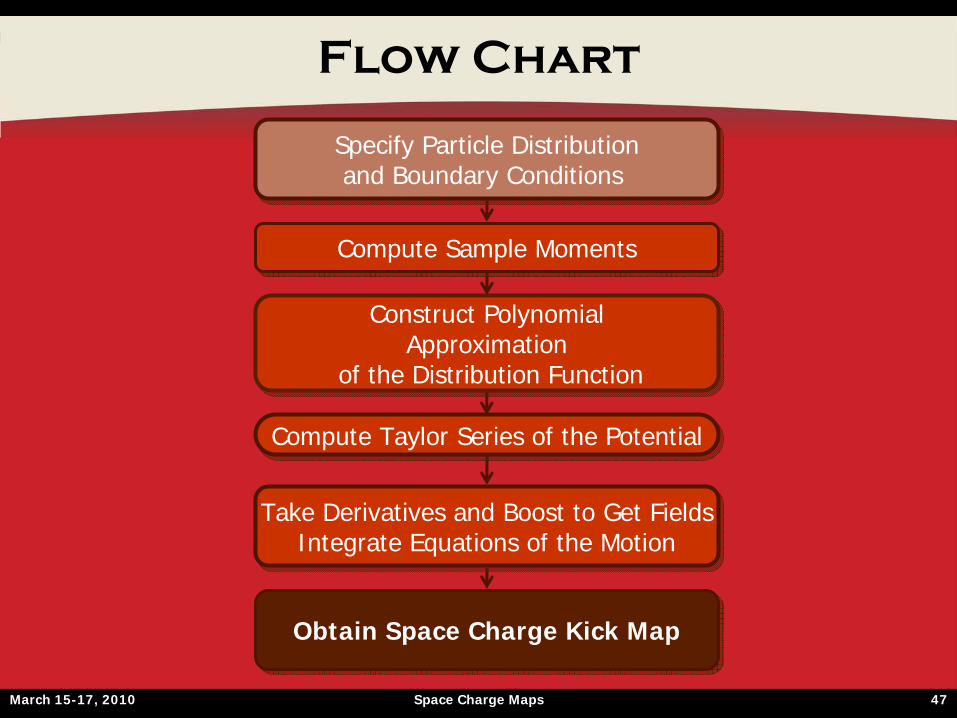
Flow Chart
Specify Particle Distributionand Boundary Conditions
Specify Particle Distributionand Boundary Conditions
Compute Sample MomentsCompute Sample Moments
Construct PolynomialApproximation
of the Distribution Function
Construct PolynomialApproximation
of the Distribution Function
Compute Taylor Series of the PotentialCompute Taylor Series of the Potential
Take Derivatives and Boost to Get FieldsIntegrate Equations of the Motion
Take Derivatives and Boost to Get FieldsIntegrate Equations of the Motion
Obtain Space Charge Kick MapObtain Space Charge Kick Map
March 15-17, 2010 Space Charge Maps 48
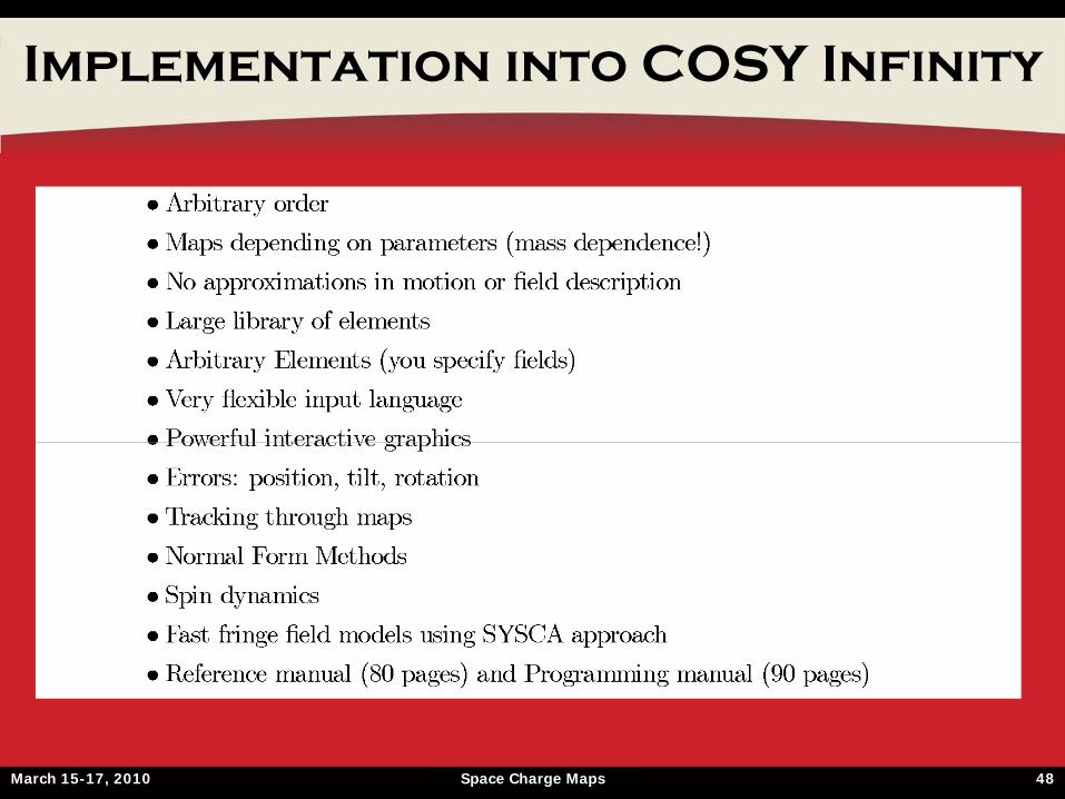
Implementation into COSY Infinity
March 15-17, 2010 Space Charge Maps 49
Implementation into COSY Infinity
• The space charge kick map is implemented as just another optical element
• Insert it anywhere is the system• Input: define aperture shape and
boundary conditions, total beam current, integration length, highest moment order to use
• Output: updates system map, coordinate system, graphics, and if instructed so applies the kicks to the particle distribution

March 15-17, 2010 Space Charge Maps 50
Map ComparisonDrift Map
Drift map with 1 space charge kick
March 15-17, 2010 Space Charge Maps 51
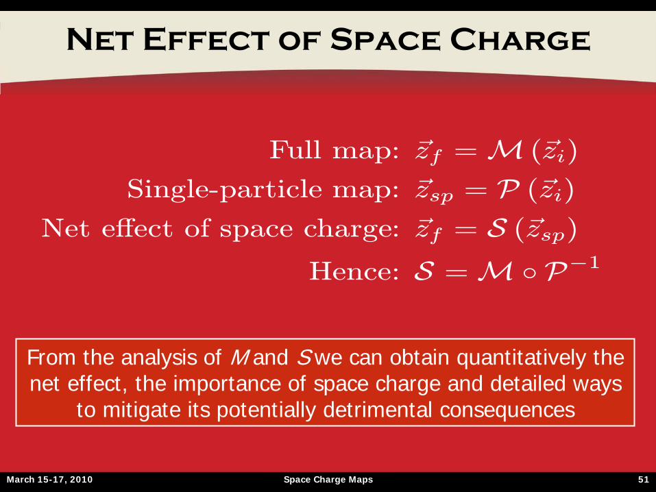
Net Effect of Space Charge
Full map: ~zf =M (~zi)
Single-particle map: ~zsp = P (~zi)Net effect of space charge: ~zf = S (~zsp)
Hence: S =M ◦ P−1
From the analysis of M and S we can obtain quantitatively the net effect, the importance of space charge and detailed ways
to mitigate its potentially detrimental consequences
March 15-17, 2010 Space Charge Maps 52
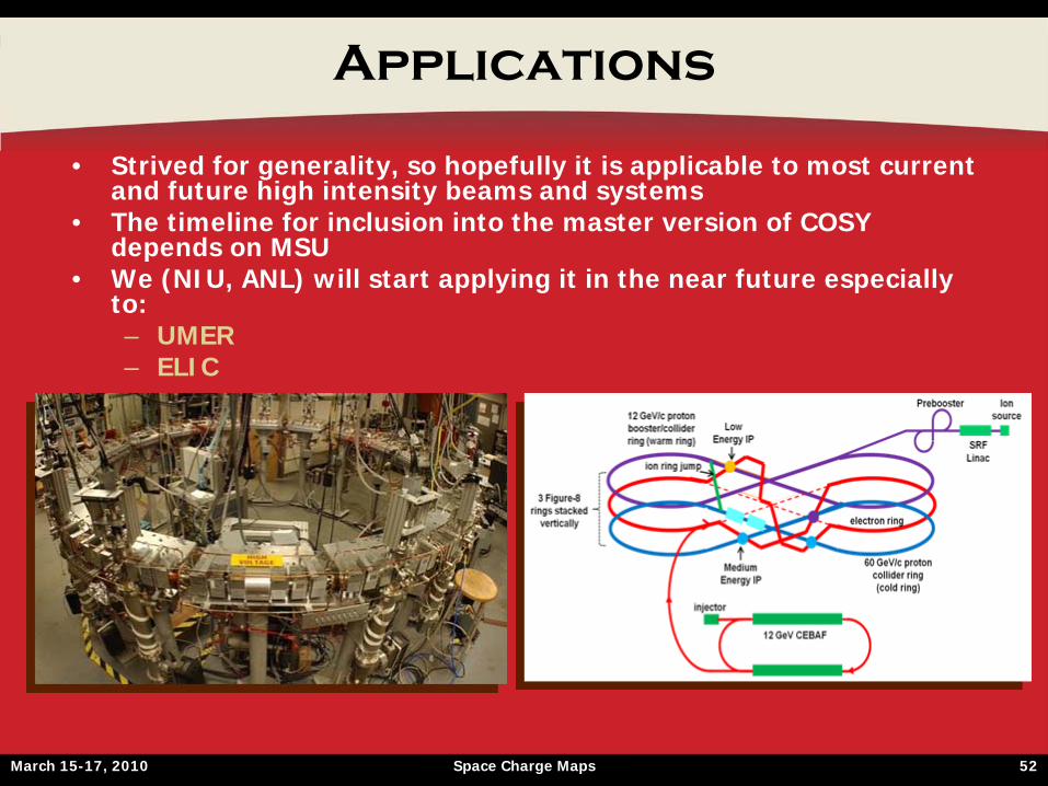
Applications
• Strived for generality, so hopefully it is applicable to most current and future high intensity beams and systems
• The timeline for inclusion into the master version of COSY depends on MSU
• We (NIU, ANL) will start applying it in the near future especially to:– UMER– ELIC
March 15-17, 2010 Space Charge Maps 53
Summary
• Developed a theory of transfer maps for beams with space charge
• Numerical experiments show excellent results for some standard distributions
• It is general and flexible enough to be useful for a wide variety of beams and accelerators, both current and future
• Implementation into COSY is proceeding• Applications to UMER and ELIC will start soon• In summary: as a consequence of the new
methods we expect significant advances in space charge related phenomena understanding and mitigation in the near future