Transfer-matrix for the multichannel scattering problem

Transfer-Matrix for the Multichannel Scattering Problem

D. M. Sedrakian

Yerevan State University, Yerevan, Armenia Received December 4, 2009

Abstract⎯A transfer-matrix for the multichannel scattering problem is obtained. The elements of this matrix are expressed in terms of transmission and reflection amplitudes. On the basis of the matrix for a system of N localized and nonoverlapped scattering centers the recurrent equations for the transfer-matrix elements are derived and the initial conditions are defined.

DOI: 10.3103/S1068337210030047 Key words: multichannel scattering problem, transfer-matrix, transmission, reflection, initial conditions

1. INTRODUCTION In works [1, 2] the problem of scattering of a quantum particle by a two-dimensional potential ( ),U x y has been considered. It was shown that it is convenient to represent the Schrödinger equation in

the form

( ) ( )( ) ( )2 2

22 2 ψ , χ , ψ , 0,x y V x y x y

x y⎛ ⎞∂ ∂

+ + − =⎜ ⎟∂ ∂⎝ ⎠ (1)

where the following notations are introduced:

( ) ( ) ( )2 2 22 χ , 2 , .m E m U V x y= = (2)

A solution to equation (1) with the boundary conditions ( ) ( ),0 ,V x V x a= =∞ is sought for in the form

( ) ( ) ( )1

ψ , ψ φ ,n

m mm

x y x y=

=∑ (3)

where ( )φm y is a solution to the equation

( ) ( )

22

2

φχ φ 0m

m m

d yy

dy+ = (4)

with ( )χ π ,m a m= 1,2,...,m n= and has the form

2 πφ sin .m mya a

⎛ ⎞= ⎜ ⎟⎝ ⎠

(5)

Note that solutions (5) are orthonormalized and, hence, satisfy the requirements

( ) ( )*i ,

0

φ φ δ .a

m m iy y dy =∫ (6)

In order to derive the desired functions ( )ψ ,m x we obtain the system of equations

( ) ( ) ( )

22

,21

ψκ ψ ψ 0, 1,2,..., ,

nm

m m m i im

d xx V x m n

dx =

+ − = =∑ (7)

where 2 2 2κ χ χ .m m= − In fact, in the y-direction a particle makes oscillations with a discrete energy, while in the x-direction it can be scattered by the potential ( ) :mnV x

ISSN 1068–3372, Journal of Contemporary Physics (Armenian Academy of Sciences), 2010, Vol. 45, No. 3, pp. 118–125. © Allerton Press, Inc., 2010. Original Russian Text © D.M. Sedrakian, 2010, published in Izvestiya NAN Armenii, Fizika, 2010, Vol. 45, No. 3, pp. 183–192.

118

TRANSFER-MATRIX

119

JOURNAL OF CONTEMPORARY PHYSICS (ARMENIAN Ac. Sci.) Vol. 45 No. 3 2010

( ) ( ) ( ) ( )0

, .a

mi m iV x y V x y y dy= ϕ ϕ∫ (8)

In works [2, 3] it was shown that the solution to the system of equations (7) and (8) leads to the determination of scattering amplitudes it and .ir In particular, in [3] a method was proposed to find these quantities depending on the form of the potential ( ),V x y and on the thickness of the scattering layer.

As was shown in [4, 5], in consideration of one-dimensional problems of scattering by the system of N nonoverlapped potentials the transfer-matrix plays an important role. This matrix connects the reflection amplitudes NR with the transmission amplitudes .NT It is of importance that, according to the transfer-matrix method, the elements of this matrix are expressed in terms of the quantities NR and .NT A knowledge of this matrix allows one to derive recurrent relations between the matrix elements, which form the basic system of algebraic difference equations for solving the problems of particle scattering by the system of potentials consisting of N links [4]. These equations may be a basis for studying the particle localization in transmission of the system of potentials lacking a high degree of periodicity [5].

The goal of this work is to generalize the results, obtained in [6] for the two-channel scattering, for the case of multichannel scattering of a quantum particle. This means to find the matrix, which connects the reflection amplitudes mR with the transmission amplitudes mT corresponding to the scattering with momenta .mk It is assumed that the particle falls on the potential ( ),V x y with momentum 1k and, hence, the first channel is characterized by the scattering amplitudes 1R and 1.T In section 2 the transfer-matrix for the multichannel scattering is derived. The elements of this matrix are expressed in terms of the scattering amplitudes mT and mR in section 3. In the last section we derive the difference equations for the transfer-matrix elements. It is shown that the problem of n-channel scattering in the case of N potentials is reduced to the solution of the system of equations studied in the problems of one-dimensional scattering [4, 5].

2. TRANSFER-MATRIX FOR THE n-CHANNEL SCATTERING Let us assume that the potential ( ),V x y has an arbitrary form along the y-axis and is nonzero in the

region 1 2.x x x≤ ≤ General solutions to equation (7) in the ranges 1x x≤ and 2x x≥ may be written in the following form: ψ , 1,2,...,ik x ik x

im im imm mA e B e m n−= + = at 1x x≤ (9)

and ψ , 1,2,...,ik x ik x

fm fm fmm mA e B e m n−= + = at 2.x x≥ (10)

A solution to this system of equations in the region 1 2x x x≤ ≤ is sought in the form ψ , 1,2,..., ,ik x ik x

m m mm ma e b e m n−= − = (11)

where ( )ma x and ( )mb x are unknown functions of x which satisfy the condition

( ) ( )( ) 2 , 1,2,..., .ik xm m

mda x dx db x dx e m n−= = (12)

Such a choice of the functions ( )ma x and ( )mb x means that, independent of the form of the potentials ( ) ,miV x the functions ( )ψm x and their first derivatives with respect to x will be continuous functions of x

only if we require a continuity of the function ( )ψm x [7]. Therefore, at joining of solutions to equation (7) at the potential boundaries 1x and 2x it is sufficient to require the continuity of the functions at these points. Before proceeding to the joining of these solutions, it should be noted that if ( )ψm x are expressed by formulas (11) and are the solutions to equations (7) then their complex-conjugate solutions will be the other linearly independent pair of solutions. The general solution of these equations can be easily derived if we multiply solutions (11) by 1L and their complex-conjugate by 2L and add. Here 1L and 2L are arbitrary constants which then are determined from the joining conditions. The obtained general solution can be represented in the following form:

( ) ( ) ( ) ( )1 2 2 1 1 2ψ , 1,2,... at .ik x ik xm m m m m

m mL a x L b x e L a x L b x e m n x x x−∗ ∗⎡ ⎤ ⎡ ⎤= − + − = ≤ ≤⎣ ⎦ ⎣ ⎦ (13)

The continuity of the functions ψm at the boundary 1x x= leads to the equations

( ) ( )( ) ( )

1 1 2 1

1 1 2 1

,

.im m m

im m m

A L a x L b x

B L b x L a x

∗

∗

= −

= − + (14)

SEDRAKIAN

120


Equations (14) give an opportunity to express the constants 1L and 2L in terms of ,imA imB and the values of ,ma mb and their complex-conjugates at the point 1.x Expressions for the constants 1L and 2L may be written in the form

( ) ( )1 1

11 ,

Δ

n

im m im mm

A a x B b xL

∗ ∗

=

⎡ ⎤+⎣ ⎦=∑

(15)

( ) ( )1 1

12 ,

Δ

n

im m im mm

A b x B a xL =

⎡ ⎤+⎣ ⎦=∑

(16)

where

( ) ( )2 21 1

1, .

n

m m m mm

a x b x=

Δ = Δ Δ = −∑

Note that at a certain normalization of the functions ma and mb one can ensure the condition 1.Δ = Proceed now to joining of the solutions ( )ψm x at the other end of the potential, 2 .x x= Conditions of

their continuity give the expressions ( ) ( )1 2 2 2 ,fm m mA L a x L b x∗= − (17)

( ) ( )1 2 2 2 .fm m mB L b x L a x∗= − + (18)

Substituting 1L and 2L from solutions (15) and (16) into equations (17) and (18), one can derive the expressions connecting the constants fmA and fmB with imA and .imB In particular, we get

( )* *

1

,n

fm mk ik mk ikk

A A B=

= α −β∑ (19)

( )1

,n

fm mk ik mk ikk

B A B=

= −β + α∑ (20)

where the following notations are used:

( ) ( ) ( ) ( ) ( )

( ) ( ) ( ) ( ) ( )

2 1 2 1*1 2

* *2 1 2 1*

1 2

, ,

, .

m k m kmk

m k m kmk

a x a x b x b xx x

a x b x b x a xx x

∗ ∗−α =

Δ− +

β =Δ

(21)

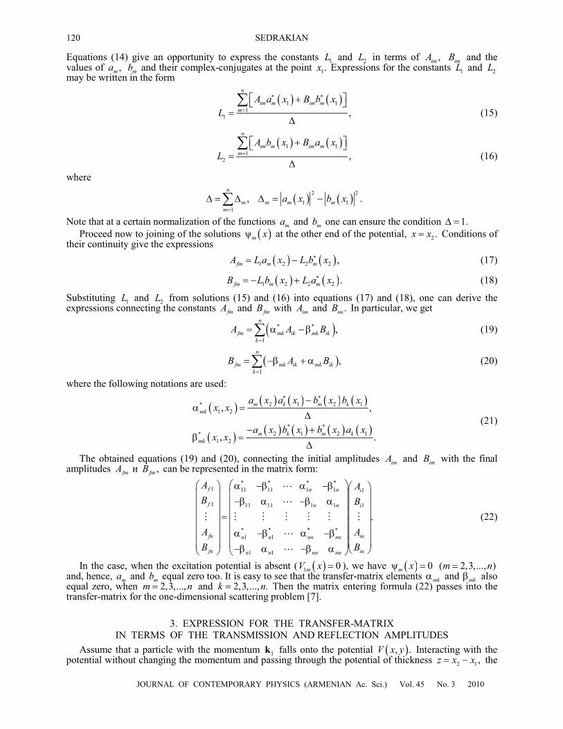
The obtained equations (19) and (20), connecting the initial amplitudes imA and imB with the final amplitudes fmA и ,fmB can be represented in the matrix form:

* * * *1 11 11 1 1 1

1 11 11 1 1 1

* * * *1 1

1 1

.

f n n i

f n n i

fn inn n nn nn

fn inn n nn nn

A AB B

A AB B

⎛ ⎞⎛ ⎞ α −β α −β ⎛ ⎞⎜ ⎟⎜ ⎟ ⎜ ⎟−β α −β α⎜ ⎟⎜ ⎟ ⎜ ⎟⎜ ⎟⎜ ⎟ ⎜ ⎟=⎜ ⎟⎜ ⎟ ⎜ ⎟⎜ ⎟α −β α −β⎜ ⎟ ⎜ ⎟⎜ ⎟⎜ ⎟ ⎜ ⎟−β α −β α ⎝ ⎠⎝ ⎠ ⎝ ⎠

(22)

In the case, when the excitation potential is absent ( ( )1 0mV x = ), we have ( )ψ 0m x = ( 2,3,..., )m n= and, hence, ma and mb equal zero too. It is easy to see that the transfer-matrix elements mkα and mkβ also equal zero, when 2,3,...,m n= and 2,3,..., .k n= Then the matrix entering formula (22) passes into the transfer-matrix for the one-dimensional scattering problem [7].

3. EXPRESSION FOR THE TRANSFER-MATRIX IN TERMS OF THE TRANSMISSION AND REFLECTION AMPLITUDES

Assume that a particle with the momentum 1k falls onto the potential ( ), .V x y Interacting with the potential without changing the momentum and passing through the potential of thickness 2 1,z x x= − the

TRANSFER-MATRIX

121


particle can transmit the potential with the amplitude 1T or be reflected with the amplitude 1.R The probability of passing of the particle through the potential has the form

2 2

1.

n

mm

T T=

=∑ (23)

One can also consider the quantity

2 2

1,

n

mm

R R=

=∑ (24)

which is the total probability of reflection and is connected with 2T by the formula

2 21 .R T= − (25) This condition follows from the conservation law for the probability flow density, which has the form

( )2 2

11.

n

m mm

T R=

+ =∑ (26)

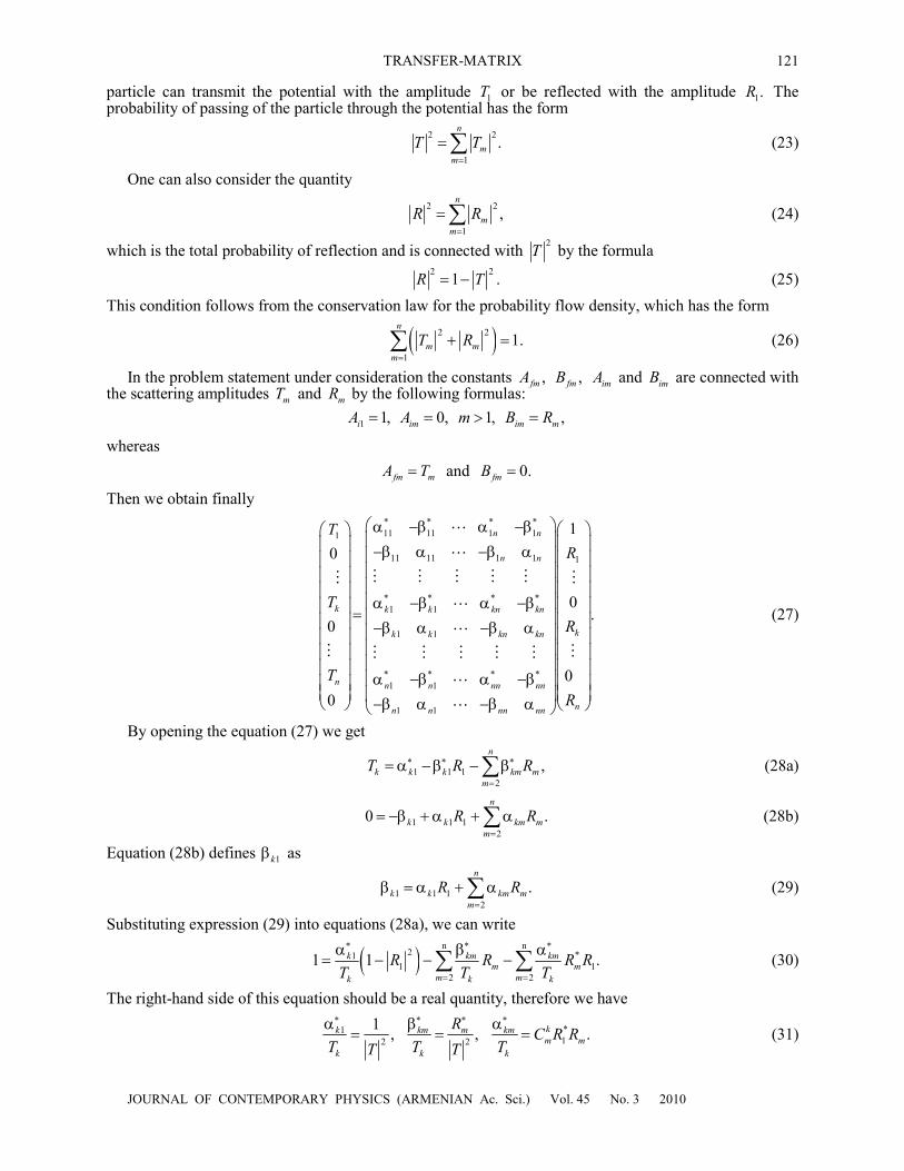
In the problem statement under consideration the constants ,fmA ,fmB imA and imB are connected with the scattering amplitudes mT and mR by the following formulas: 1 1, 0, 1, ,i im im mA A m B R= = > =

whereas fm mA T= and 0.fmB =

Then we obtain finally

* * * *11 11 1 11

11 11 1 1

* * * *1 1

1 1

* * * *1 1

1 1

0

0

0

n n

n n

k k k kn kn

k k kn kn

n n n nn nn

n n

T

T

T

α −β α −β⎛ ⎞⎜ ⎟ −β α −β α⎜ ⎟⎜ ⎟⎜ ⎟

α −β α −β⎜ ⎟ =⎜ ⎟ −β α −β α⎜ ⎟⎜ ⎟⎜ ⎟

α −β α −β⎜ ⎟⎜ ⎟ −β α −β⎝ ⎠

1

1

0

.

0

k

nnn nn

R

R

R

⎛ ⎞⎛ ⎞⎜ ⎟⎜ ⎟⎜ ⎟⎜ ⎟⎜ ⎟⎜ ⎟⎜ ⎟⎜ ⎟⎜ ⎟⎜ ⎟⎜ ⎟⎜ ⎟⎜ ⎟⎜ ⎟⎜ ⎟⎜ ⎟⎜ ⎟⎜ ⎟⎜ ⎟⎜ ⎟

⎜ ⎟⎜ ⎟α ⎝ ⎠⎝ ⎠

(27)

By opening the equation (27) we get

1 1 12

,n

k k k km mm

T R R∗ ∗ ∗

=

= α −β − β∑ (28a)

1 1 12

0 .n

k k km mm

R R=

= −β +α + α∑ (28b)

Equation (28b) defines 1kβ as

1 1 12

.n

k k km mm

R R=

β = α + α∑ (29)

Substituting expression (29) into equations (28a), we can write

( )n n

2 *11 1

2 21 1 .k km km

m mm mk k k

R R R RT T T

∗ ∗ ∗

= =

α β α= − − −∑ ∑ (30)

The right-hand side of this equation should be a real quantity, therefore we have

*112 2

1 , , .kk km m kmm m

k k k

R C R RT T TT T

∗ ∗ ∗ ∗α β α= = = (31)

SEDRAKIAN

122


Substituting expressions (31) into formula (30), we derive

2 2 212

1 2

11 1 .n n

km m m

m mR C R R

T = =

⎛ ⎞= − −⎜ ⎟

⎝ ⎠∑ ∑ (32)

Taking into account that equation (32) should pass into formula (26), we must require that 0kmC = at

2,..., .m n= From this requirement and equation (31) it follows that 0kmα = for all k and 2,..., .m n= Thus, only the function 1kα is nonzero, which we denote by .kα Then, according to formulas (31), we have

( ) ( )2 21 , .k k k km m k kT T T R T T Tα = β = (33a) Analogously we can separate 1kβ from kmβ and introduce the notations

2 2

11 , .k m k

k k km kmk k

T R TRT T T T

β = β = β ≡ δ = (33b)

Then the system of equations (27) can be written in the form

* * * *1 1 12 11

1 1 12 1

* * * *2

2

0 00 00

0 0

0 0 0

0

n

n

k k k k kn

k k k kn

n

T

T

T

α −β − δ −δ⎛ ⎞⎜ ⎟ −β α −δ −δ⎜ ⎟⎜ ⎟⎜ ⎟

α −β − δ −δ⎜ ⎟ =⎜ ⎟ −β α −δ −δ⎜ ⎟⎜ ⎟⎜ ⎟⎜ ⎟⎜ ⎟⎝ ⎠

1

* * * *2

2

1

0

,

00 0

0 0

k

n n n nn

nn n n nn

R

R

R

⎛ ⎞⎛ ⎞⎜ ⎟⎜ ⎟⎜ ⎟⎜ ⎟⎜ ⎟⎜ ⎟⎜ ⎟⎜ ⎟⎜ ⎟⎜ ⎟⎜ ⎟⎜ ⎟⎜ ⎟⎜ ⎟⎜ ⎟⎜ ⎟⎜ ⎟⎜ ⎟α −β − δ −δ⎜ ⎟⎜ ⎟

⎜ ⎟⎜ ⎟−β α −δ −δ ⎝ ⎠⎝ ⎠

(34)

where, as was noted, the transfer-matrix elements are expressed in terms of the transmission and reflection amplitudes by formulas (33a) and (33b).

Finally we note that the following relations are fulfilled:

2 2 2 2 2

1 11 , ,

n n

k kmk k

T R T= =

α = β =∑ ∑

and, hence, according to expression (25), we have

2 2

1 21.

n n

k kmk m= =

⎛ ⎞α − β =⎜ ⎟⎝ ⎠

∑ ∑ (35)

Note also that the transfer-matrix elements kmβ are expressed in terms of kα and mR by the relation .km k mRβ = α

4. DIFFERENCE EQUATION FOR THE TRANSFER-MATRIX ELEMENTS Let us consider the problem of motion of a quantum particle in the x-direction in the field of a chain

consisting of a finite number of scattering centers. Let a model potential of the problem considered have the following form:

( ) ( )1

, , ,N

i ii

U x y U x x y=

= −∑ (36)

where N is the number of scatterers in the chain, ( ),i iU x x y− are nonoverlapped functions localized near the points ix ( )1,2,... .i N= If the parameters 1 2, , ... Nx x x characterizing the disposition of scatterers in space, satisfy the condition ( )1 1 ,ix x i b= + − then we have the chain of periodically located scatterers. If, along with this, the fields, created by different scatterers, are identical then the chain consists of periodically disposed, identical potentials. However, one can consider the problem in the most general form when the scatterers are not identical and a periodicity in their disposition is absent. According to the matrix method, developed in section 3, we can write

TRANSFER-MATRIX

123


( ) ( ) ( ) ( )( ) ( ) ( ) ( )( ) ( ) ( ) ( )( ) ( ) ( )

* * * *1 1 12 1

1

1 1 12 1

* * * *2 2 22 22

2 2 22

0 0

0 00 0 0

0

0

nN

n

nN

nN

i i i iT

i i i i

i i i iTi i i

T

α −β − δ − δ⎛ ⎞⎜ ⎟ −β α −δ −δ⎜ ⎟

α −β − δ − δ⎜ ⎟⎜ ⎟

= −β α −δ⎜ ⎟⎜ ⎟⎜ ⎟⎜ ⎟⎜ ⎟⎝ ⎠

( )

( ) ( ) ( ) ( )( ) ( ) ( ) ( )

2

* * * *2

2

0 0

0 i 0

0 0

n

n n n nn

n n n nn

i

i i i

i i i i

⎛⎜⎜⎜⎜⎜ −δ⎜⎜⎜α −β − δ − δ

−β α − δ −δ⎝

1

1

2

1

0 , 0

N

Ni N

nN

R

R

R

=

⎞⎛ ⎞⎟⎜ ⎟⎟⎜ ⎟⎟⎜ ⎟⎟⎜ ⎟⎟⎜ ⎟⎟⎜ ⎟⎟⎜ ⎟⎟⎜ ⎟⎜ ⎟⎜ ⎟⎜ ⎟⎝ ⎠⎜ ⎟⎠

∏ (37)

where ( ) ,k iα ( )k iβ and ( ),k m iδ are the transfer-matrix elements from the i-th scatterer of the chain in the absence of all other scatterers. Note that the transfer-matrices entering formula (37) are commuting, when scatterers in the chain are identical and disposed equidistantly. It is essential that the transfer-matrix elements in formula (37) should be calculated with allowance for the disposition of scatterers.

Now we will show that the problem of determination of the amplitudes iNT and iNR for the multichannel scattering of a particle can be, in the general form, reduced to the solution of the system of 3n linear difference equations of the first order, where n is the number of channels. With this aim we introduce the transfer-matrix for the whole chian:

( ) ( ) ( ) ( )( ) ( ) ( ) ( )

( ) ( ) ( ) ( )( ) ( ) ( )

* * * *1 1 12 1

1

1 1 12 1

* * * *2 2 22 22

2 2 22

0 0

0 00 0 0

0

0

nN

n

nN

nN

S N D N M N M NT

D N S N M N M N

S N D N M N M NTD N S N M N

T

− − −⎛ ⎞⎜ ⎟ − − −⎜ ⎟

− − −⎜ ⎟⎜ ⎟

= − −⎜ ⎟⎜ ⎟⎜ ⎟⎜ ⎟⎜ ⎟⎝ ⎠

( )

( ) ( ) ( ) ( )( ) ( ) ( ) ( )

2

* * * *2

2

0 0

0 0

0

n

n n n nn

n n n nn

M N

S N D N M N M N

D N S N M N M N

−

− − −

− − −

1

2

1

0.

0

0

N

N

nN

R

R

R

⎛ ⎞⎛ ⎞⎜ ⎟⎜ ⎟⎜ ⎟⎜ ⎟⎜ ⎟⎜ ⎟⎜ ⎟⎜ ⎟⎜ ⎟⎜ ⎟⎜ ⎟⎜ ⎟⎜ ⎟⎜ ⎟⎜ ⎟⎜ ⎟⎜ ⎟⎜ ⎟⎜ ⎟⎝ ⎠⎜ ⎟

⎝ ⎠

(38)

Here for the chain consisting of N scatterers we used the transfer-matrix entering formula (27), introducing the notations ( ) ,S N ( )D N and ( )M N instead of ikα and .ikβ Comparison of formulas (37) and (38) shows that the matrix entering expression (38) is calculated as a product of the transfer-matrix for separate scatterers of the chain. Consider the transfer-matrix elements ( ) ,mS N ( ) ,mD N and

( )kmM N as functions of a discrete parameter N so that ( )1 ,mS N − ( )1 ,mD N − and ( )1kmM N − should correspond to the matrix elements in passing of the particle along the first N – 1 potentials of the chain. It is easy to see that between the transfer-matrix elements of the whole chain and the chain without the last potential the following relation exists:

( ) ( ) ( )( ) ( ) ( )

( ) ( ) ( )( ) ( ) ( )

1 1 1

1 1 1

* * *1 1 1

1 1 1

* * *

00

0

0

00

00

n

n

n n nn

n n nn N

n

n

n n mn

n n nn

S D MD S M

S D MD S M

N N NN N N

N N NN N N

∗ ∗ ∗

∗ ∗ ∗

⎛ ⎞− −⎜ ⎟− −⎜ ⎟

⎜ ⎟ =⎜ ⎟

− −⎜ ⎟⎜ ⎟− −⎝ ⎠

⎛ ⎞α −β −δ⎜ ⎟−β α −δ⎜ ⎟

⎜ ⎟=⎜ ⎟α −β −δ⎜ ⎟

⎜ ⎟−β α −δ⎝ ⎠

1 1 1

1 1 1

1

00

.0

0

n

n

n n nn

n n nn N

S D MD S M

S D MD S M

∗ ∗ ∗

∗ ∗ ∗

−

⎛ ⎞− −⎜ ⎟− −⎜ ⎟

⎜ ⎟⎜ ⎟

− −⎜ ⎟⎜ ⎟− −⎝ ⎠

(39)

SEDRAKIAN

124


Note that the law of conservation of the probability flow density, expressed in terms of the quantities S, D, and M, has the form

( ) ( ) ( )2 2 2

1 11.

n n

m m mkm k

S N D N M N= =

⎛ ⎞− − =⎜ ⎟

⎝ ⎠∑ ∑ (40)

Considering in formula (39) N as a variable quantity, equality (39) can be represented in the form of the following system of linear difference equations of the first order:

( ) ( ) ( ) ( ) ( ) ( ) ( )

( ) ( ) ( ) ( ) ( ) ( ) ( )

( ) ( ) ( )

1 12

1 12

1

1 1 1 ,

1 1 1 ,

1 .

n

k k k km mm

n

k k k km mm

km k m

S N N S N N D N N D N

D N N D N N S N N S N

M N N M N

∗ ∗

=

∗ ∗

=

= α − +β − + δ −

= α − +β − + δ −

= α −

∑

∑ (41)

Here 1N ≥ and the initial conditions have the following form: ( ) ( ) ( ) ( ) ( ) ( ) ( )1 1 1 1 10 1, 0 =0, 0 δ 1 1 , 0 0 0, 1.m m m mS D M S D m= = α = = ≥ (42) Thus, the system of difference equations (41) with initial conditions (42) determines the amplitudes of transmission ( )mT N and reflection ( )mR N for the system of potentials (36).

Finally we transform the system of equations (41), using formulas (33) and rewriting them for the last N-th potential in the form

( )( ) ( ) ( )

( ) ( )1 , .k kmm

k k

N NR N R N

N Nβ δ

= =α α

(43)

By substituting them into the system of equations (41) we derive

( ) ( ) ( ) ( ) ( ) ( ) ( )

( ) ( ) ( ) ( ) ( ) ( ) ( )

( ) ( ) ( )

1 1 12

1 1 12

1

1 1 1 ,

1 1 1 ,

1 .

n

k k m mm

n

k k m mm

km k m

S N N S N R N D N R N D N

D N N D N R N S N R N S N

M N N M N

∗ ∗

=

∗ ∗

=

⎡ ⎤= α − + − + −⎢ ⎥

⎣ ⎦⎡ ⎤

= α − + − + −⎢ ⎥⎣ ⎦

= α −

∑

∑ (44)

From the system of equations (44) we get

( )( )

( )( )

( )( )

( )( )1 1 1 1

.k k km k

m

S N D N M N NS N D N M N N

α= = =

α (45)

This means that it is sufficient to determine ( )1 ,S N ( )1 ,D N and ( )1 ,mM N and then unknown functions ( ) ,kS N ( ) ,kD N and ( )kmM N will be determined from relations (45). Let us write the equations for determining ( )1 ,S N ( )1 ,D N and ( )1 .mM N They can be obtained from

the system of equations (44), if we replace ( )kS N and ( )kD N by ( )1S N and ( )1D N using formulas (45). Finally we obtain

( ) ( ) ( ) ( ) ( ) ( )( ) ( ) ( ) ( ) ( ) ( )

1 1 1 1 1 1

1 1 1 1 1 1

1 1 ,

1 1 ,

S N N S N N r N D N

D N N D N N r N S N

∗

∗

= α − +α −

= α − + α − (46)

where

( ) ( ) ( ) ( )( ) ( )1 1

2 1 1

11 .

1

nm m

m

R N T Nr N R N

R N T N=

⎡ ⎤−= +⎢ ⎥

−⎢ ⎥⎣ ⎦∑ (47)

The unknown function ( )1mM N is determined from the equation ( ) ( ) ( )1 1 1 1 ,m mM N N M N= α − (48) which enters the system of equations (41).

TRANSFER-MATRIX

125


Note that the system of equations (46) coincides with the system of equations derived for the one-dimensional scattering problem, but the coefficients before the functions ( )1 1S N − and ( )1 1D N − are other. The solution of such a system has been studied in [4, 5].

REFERENCES 1. Boese, D., Lischka, M., and Reichl, L.E., Phys. Rev. B, 2000, vol. 82, p. 16933. 2. Sedrakian, D.M., Kazaryan, E.M., and Sedrakian, L.R., J. Contemp. Phys. (Armenian Ac. Sci.), 2009, vol. 44, p.

257. 3. Sedrakian, L.R., Doklady NAN Armenii, 2009, vol. 109, p. 214. 4. Sedrakian, D.M. and Khachatrian, A.Zh., Dokladi NAN Armenii, 1998, vol. 109, p. 214. 5. Sedrakian, D.M., Badalyan, D.A., Khachatrian, A.Zh., FTT, 1999, vol. 41, p. 1687. 6. Sedrakian, D.M., J. Contemp. Phys. (Armenian Ac. Sci.), 2010, vol. 45, p. 25. 7. Khachatrian, A.Zh., Sedrakian, D.M., and Khoetsyan, V.A., J. Contemp. Phys. (Armenian Ac. Sci.), 2009, vol.

44, p. 91.

Documents

Transfer-matrix for the multichannel scattering problem