Transfer-matrix for the two-channel scattering problem

Transfer-Matrix for the Two-Channel Scattering Problem

D. M. Sedrakian

Yerevan State University, Yerevan, Armenia

Received April 1, 2009

AbstractThe transfer-matrix for the two-channel scattering problem is obtained. The elements of this matrix are expressed in terms of transmission 1T , 2T and reflection 1R , 2R amplitudes. The transfer-matrix for N localized and nonoverlapping scattering centers is presented. Recurrent equations for matrix elements are derived and initial conditions for them are defined.

DOI: 10.3103/S1068337210010056

Key words: two-channel scattering, transfer-matrix, transmission, reflection

1. INTRODUCTION

In [1, 2] the problem of scattering of a quantum particle by a two-dimensional potential ,U x y has been formulated. It was shown that the Schrödinger equation can be represented in the convenient form

2 2

22 2

, χ , , 0,x y V x y x yx y

(1)

where the following notations are introduced:

22 2

2 2χ , , .

m mE U V x y

(2)

A solution to equation (1) witn the boundary conditions ,0 ,V x V x a is sought for in the form

1

, φn nn

x y x y

(3)

where φn y is the solution to the equation

22

2

φχ φ 0,n

n n

d yy

dy (4)

with χ π , 1,2,...n n a n and has the form

2 π

φ sin .n nya a

(5)

Note, that solutions (5) are orthonormalized and, hence, satisfy the requirment

*,

0

φ φ δ .a

m n m ny y dy (6)

To obtain the desired functions ψ ,n x the following system of equations is derived:

22

,21

κ 0,nn n m n m

m

d xx V x

dx

(7)

where 2 2 2κ χ χ .n n In fact, a particle makes a vibrational motion with a discrete energy 2 2χ 2n nE m in the y-direction, while in the x-direction it can be scattered by the potential .mnV x

ISSN 1068–3372, Journal of Contemporary Physics (Armenian Academy of Sciences), 2010, Vol. 45, No. 1, pp. 25–32. © Allerton Press, Inc., 2010. Original Russian Text © D.M. Sedrakian, 2010, published in Izvestiya NAN Armenii, Fizika, 2010, Vol. 45, No. 1, pp. 39–49.

25

SEDRAKIAN

26

JOURNAL OF CONTEMPORARY PHYSICS (ARMENIAN Ac. Sci.) Vol. 45 No. 1 2010

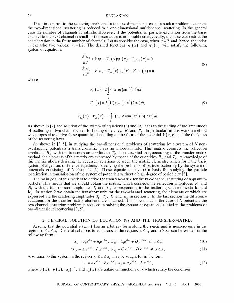
Thus, in contrast to the scattering problems in the one-dimensional case, in such a problem statement the two-dimensional scattering is reduced to a one-dimensional multichannel scattering. In the general case the number of channels is infinite. However, if the potential of particle excitation from the basic channel to the next channel is small or this excitation is impossible energetically, then one can restrict the consideration to the finite number of channels. Let us consider the case, when 2n and, hence, the index m can take two values: 1,2.m The desired functions 1ψ x and 2ψ x will satisfy the following system of equations:

221

1 1 11 1 12 22

2222 2 22 2 21 12

0,

0,

dk V x x V x

dx

dk V x x V x

dx

(8)

where

12

11

0

12

22

0

1

12 21

0

2 , sin π ,

2 , sin 2π ,

2 , sin π sin 2π .

V x V x at t dt

V x V x at t dt

V x V x V x at t t dt

(9)

As shown in [2], the solution of the system of equations (8) and (9) leads to the finding of the amplitudes of scattering in two channels, i.e., to finding of 1 2 1, , T T R and 2.R In particular, in this work a method was proposed to derive these quantities depending on the form of the potential ,V x y and the thickness of the scattering layer.

As shown in [3–5], in studying the one-dimensional problems of scattering by a system of N non-overlapping potentials a transfer-matrix plays an important role. This matrix connects the reflection amplitude NR with the transmission amplitudes .NT It is essential that, according to the transfer-matrix method, the elements of this matrix are expressed by means of the quantities NR and .NT A knowledge of this matrix allows deriving the recurrent relations between the matrix elements, which form the basic system of algebraic difference equations for solving the problems of particle scattering by the system of potentials consisting of N channels [3]. These equations may be a basis for studying the particle localization in transmission of the system of potentials without a high degree of periodicity [5].

The main goal of this work is to derive the transfer-matrix for the two-channel scattering of a quantum particle. This means that we should obtain the matrix, which connects the reflection amplitudes 1R and

2R with the transmission amplitudes 1T and 2 ,T corresponding to the scattering with momenta 1k and 2.k In section 2 we obtain the transfer-matrix for the two-channel scattering, the elements of which are

expressed via the scattering amplitudes 1 2 1, , T T R and 2R in section 3. In the last section the difference equations for the transfer-matrix elements are obtained. It is shown that in the case of N potentials the two-channel scattering problem is reduced to solving the system of equations studied in the problems of one-dimensional scattering [3, 5].

2. GENERAL SOLUTION OF EQUATION (8) AND THE TRANSFER-MATRIX

Assume that the potential ,V x y has an arbitrary form along the y-axis and is nonzero only in the region 1 2.x x x General solutions to equations in the regions 1x x and 2x x can be written in the following form:

1 1 2 21 1 1 2 1 1 1, atik x ik x ik x ik xi iA e B e C e D e x x (10)

1 1 2 21 2 2 2 2 2 2, atik x ik x ik x ik x

f fA e B e C e D e x x (11)

A solution to this system in the region 1 2x x x may be sought for in the form

1 1 2 21 1 1 2 2 2, ,ik x ik x ik x ik xa e b e a e b e (12)

where 1 1 2, , ,a x b x a x and 2b x are unknown functions of x which satisfy the condition

TRANSFER-MATRIX

27


2 , 1,2.i i ik xi

da x db xe i

dx dx (13)

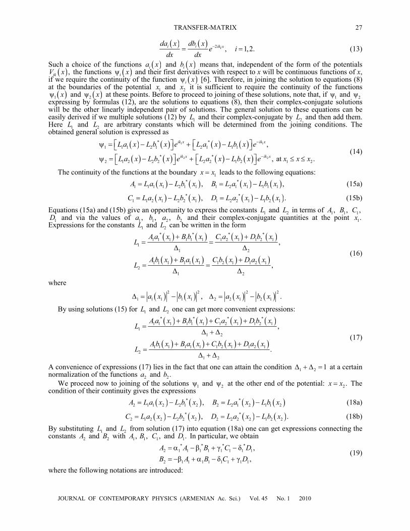
Such a choice of the functions ia x and ib x means that, independent of the form of the potentials ,ikV x the functions ψi x and their first derivatives with respect to x will be continuous functions of x,

if we require the continuity of the function ψi x [6]. Therefore, in joining the solution to equations (8) at the boundaries of the potential 1x and 2x it is sufficient to require the continuity of the functions

1ψ x and 2ψ x at these points. Before to proceed to joining of these solutions, note that, if 1ψ and 2ψ expressing by formulas (12), are the solutions to equations (8), then their complex-conjugate solutions will be the other linearly independent pair of solutions. The general solution to these equations can be easily derived if we multiple solutions (12) by 1L and their complex-conjugate by 2L and then add them. Here 1L and 2L are arbitrary constants which will be determined from the joining conditions. The obtained general solution is expressed as

1 1

2 2

* *1 1 1 2 1 2 1 1 1

* *2 1 2 2 2 2 2 1 2 1 2

,

, at .

ik x ik x

ik x ik x

L a x L b x e L a x L b x e

L a x L b x e L a x L b x e x x x

(14)

The continuity of the functions at the boundary 1x x leads to the following equations:

* *1 1 1 1 2 1 1 1 2 1 1 1 1 1, ,A L a x L b x B L a x L b x (15a)

* *1 1 2 1 2 2 1 1 2 2 1 1 2 1, .C L a x L b x D L a x L b x (15b)

Equations (15a) and (15b) give an opportunity to express the constants 1L and 2L in terms of 1,A 1,B 1,C 1D and via the values of 1,a 1,b 2 ,a 2b and their complex-conjugate quantities at the point 1.x

Expressions for the constants 1L and 2L can be written in the form

* * * *1 1 1 1 1 1 1 2 1 1 2 1

11 2

1 1 1 1 1 1 1 2 1 1 2 12

1 2

,Δ Δ

,Δ Δ

A a x B b x C a x D b xL

A b x B a x C b x D a xL

(16)

where

2 2 2 2

1 1 1 1 1 2 2 1 2 1, .a x b x a x b x

By using solutions (15) for 1L and 2L one can get more convenient expressions:

* * * *1 1 1 1 1 1 1 2 1 1 2 1

11 2

1 1 1 1 1 1 1 2 1 1 2 12

1 2

,

.

A a x B b x C a x D b xL

A b x B a x C b x D a xL

(17)

A convenience of expressions (17) lies in the fact that one can attain the condition 1 2 1 at a certain normalization of the functions 2a and 2.b

We proceed now to joining of the solutions 1ψ and 2ψ at the other end of the potential: 2 .x x The condition of their continuity gives the expressions

* *2 1 1 2 2 1 2 2 2 1 2 1 1 2, A L a x L b x B L a x L b x (18a)

* *2 1 2 2 2 2 2 2 2 2 2 1 2 2, .C L a x L b x D L a x L b x (18b)

By substituting 1L and 2L from solution (17) into equation (18a) one can get expressions connecting the constants 2A and 2B with 1,A 1,B 1,C and 1.D In particular, we obtain

* * * *

2 1 1 1 1 1 1 1 1

2 1 1 1 1 1 1 1 1

β γ δ ,

β δ γ ,

A A B C D

B A B C D

(19)

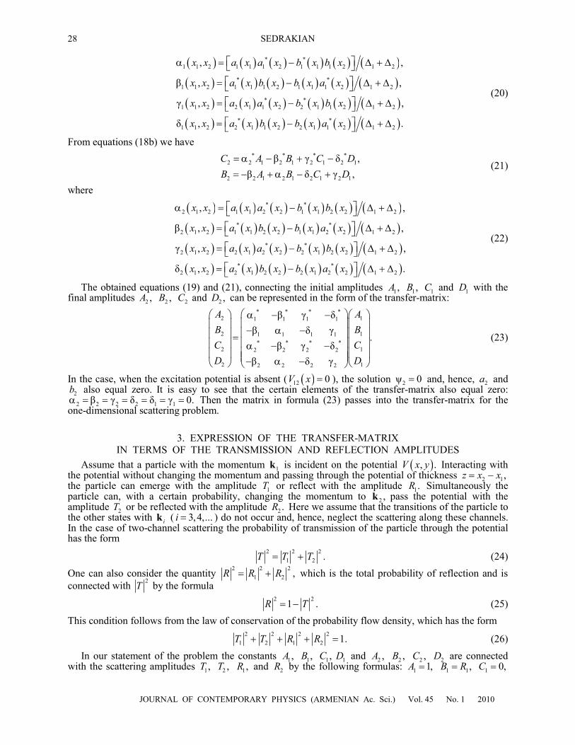
where the following notations are introduced:

SEDRAKIAN

28


* *1 1 2 1 1 1 2 1 1 1 2 1 2

* *1 1 2 1 1 1 2 1 1 1 2 1 2

* *1 1 2 2 1 1 2 2 1 1 2 1 2

* *1 1 2 2 1 1 2 2 1 1 2 1 2

, ,

β , ,

γ , ,

δ , .

x x a x a x b x b x

x x a x b x b x a x

x x a x a x b x b x

x x a x b x b x a x

(20)

From equations (18b) we have

* * * *

2 2 1 2 1 2 1 2 1

2 2 1 2 1 2 1 2 1

β γ δ ,

β δ γ ,

C A B C D

B A B C D

(21)

where

* *2 1 2 1 1 2 2 1 1 2 2 1 2

* *2 1 2 1 1 2 2 1 1 2 2 1 2

* *2 1 2 2 1 2 2 2 1 2 2 1 2

* *2 1 2 2 1 2 2 2 1 2 2 1 2

, ,

β , ,

γ , ,

δ , .

x x a x a x b x b x

x x a x b x b x a x

x x a x a x b x b x

x x a x b x b x a x

(22)

The obtained equations (19) and (21), connecting the initial amplitudes 1,A 1,B 1C and 1D with the final amplitudes 2 ,A 2 ,B 2C and 2 ,D can be represented in the form of the transfer-matrix:

* * * *2 11 1 1 1

2 11 1 1 1* * * *

2 12 2 2 2

2 12 2 2 2

β γ δ

β δ γ.

β γ δ

β δ γ

A A

B B

C C

D D

(23)

In the case, when the excitation potential is absent ( 12 0V x ), the solution 2ψ 0 and, hence, 2a and 2b also equal zero. It is easy to see that the certain elements of the transfer-matrix also equal zero: 2 2 2 2 1 1β γ δ δ γ 0. Then the matrix in formula (23) passes into the transfer-matrix for the

one-dimensional scattering problem.

3. EXPRESSION OF THE TRANSFER-MATRIX IN TERMS OF THE TRANSMISSION AND REFLECTION AMPLITUDES

Assume that a particle with the momentum 1k is incident on the potential , .V x y Interacting with the potential without changing the momentum and passing through the potential of thickness 2 1,z x x the particle can emerge with the amplitude 1T or reflect with the amplitude 1.R Simultaneously the particle can, with a certain probability, changing the momentum to 2 ,k pass the potential with the amplitude 2T or be reflected with the amplitude 2.R Here we assume that the transitions of the particle to the other states with ik ( 3,4,...i ) do not occur and, hence, neglect the scattering along these channels. In the case of two-channel scattering the probability of transmission of the particle through the potential has the form

2 2 2

1 2 .T T T (24)

One can also consider the quantity 2 2 2

1 2 ,R R R which is the total probability of reflection and is connected with

2T by the formula

2 2

1 .R T (25)

This condition follows from the law of conservation of the probability flow density, which has the form

2 2 2 2

1 2 1 2 1.T T R R (26)

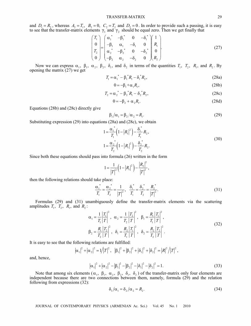
In our statement of the problem the constants 1,A 1,B 1,C 1D and 2 ,A 2 ,B 2 ,C 2D are connected with the scattering amplitudes 1,T 2 ,T 1,R and 2R by the following formulas: 1 1,A 1 1,B R 1 0,C

TRANSFER-MATRIX

29


and 1 2D R , whereas 2 1,A T 2 0,B 2 2C T and 2 0D . In order to provide such a passing, it is easy to see that the transfer-matrix elements 1γ and 2γ should be equal zero. Then we get finally that

* * *1 1 1 1

11 1 1* * *

2 2 2 2

22 2 2

1β 0 δ

0 β δ 0.

0β 0 δ

0 β δ 0

T

R

T

R

(27)

Now we can express 1, 1β , 2 , 2β , 1δ , and 2δ in terms of the quantities 1,T 2 ,T 1,R and 2R . By opening the matrix (27) we get

* * *1 1 1 1 1 2β δ ,T R R (28a)

1 1 10 β + ,R (28b)

* * *2 2 2 1 2 2β δ ,T R R (28c)

2 2 10 β .R (28d)

Equations (28b) and (28c) directly give

1 1 2 2 1β β .R (29)

Substituting expression (29) into equations (28a) and (28c), we obtain

* *21 1

1 21 1

* *22 2

1 22 2

δ1 1 ,

δ1 1 .

R RT T

R RT T

(30)

Since both these equations should pass into formula (26) written in the form

2

2 212 2

11 1 ,

RR

T T

then the following relations should take place:

* * * * *

1 2 1 2 22 2

1 2 1 2

δ δ1, .

R

T T T TT T

(31)

Formulas (29) and (31) unambiguously define the transfer-matrix elements via the scattering amplitudes 1,T 2 ,T 1,R and 2R :

2 2 2

1 2 1 11 2 1

1 2 1

2 2 2

1 2 2 1 2 22 1 2

2 1 2

1 1, , β ,

β , δ , δ .

T T R T

T T T T T T

R T R T R T

T T T T T T

(32)

It is easy to see that the following relations are fulfilled:

2 2 2 2 2 2 2 2 2

1 2 1 2 1 21 , β β δ δ ,T R T

and, hence,

2 2 2 2 2 2

1 2 1 2 1 2β β δ δ 1. (33)

Note that among six elements ( 1, 1β , 2 , 2β , 1δ , 2δ ) of the transfer-matrix only four elements are independent because there are two connections between them, namely, formula (29) and the relation following from expressions (32):

1 1 2 2 2δ δ .R (34)

SEDRAKIAN

30


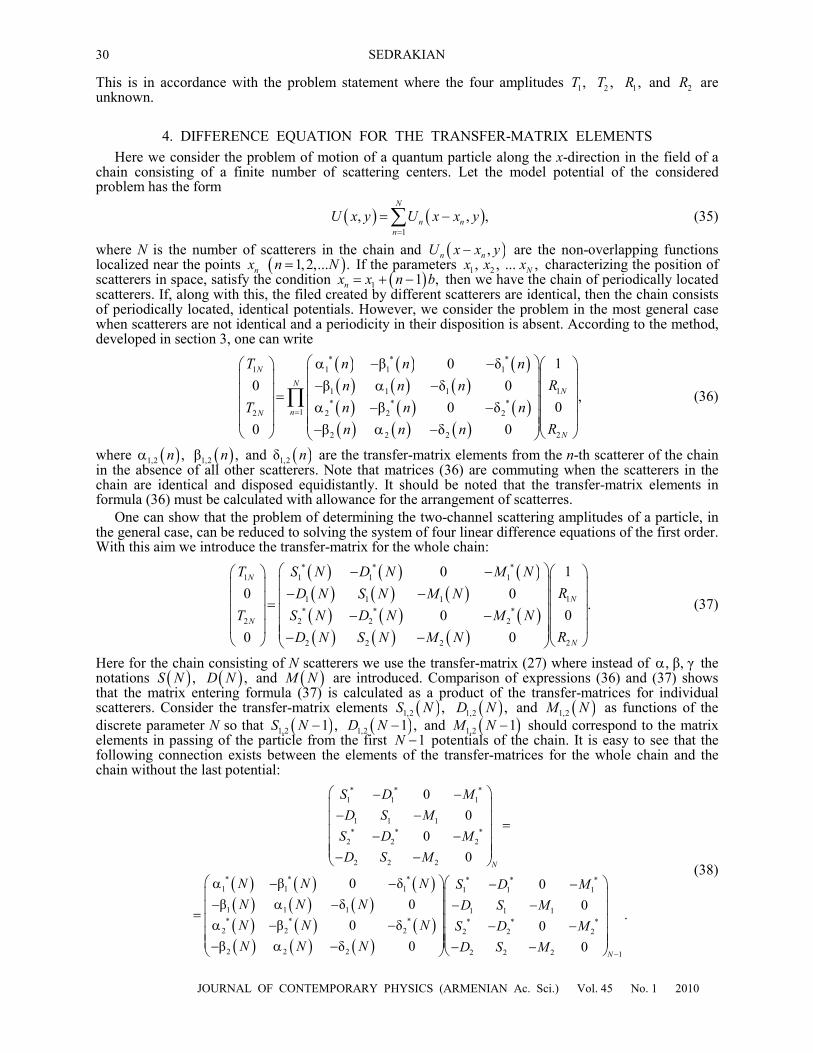
This is in accordance with the problem statement where the four amplitudes 1,T 2 ,T 1,R and 2R are unknown.

4. DIFFERENCE EQUATION FOR THE TRANSFER-MATRIX ELEMENTS

Here we consider the problem of motion of a quantum particle along the x-direction in the field of a chain consisting of a finite number of scattering centers. Let the model potential of the considered problem has the form

1

, , ,N

n nn

U x y U x x y

(35)

where N is the number of scatterers in the chain and ,n nU x x y are the non-overlapping functions localized near the points nx 1,2,... .n N If the parameters 1 2, , ... ,Nx x x characterizing the position of scatterers in space, satisfy the condition 1 1 ,nx x n b then we have the chain of periodically located scatterers. If, along with this, the filed created by different scatterers are identical, then the chain consists of periodically located, identical potentials. However, we consider the problem in the most general case when scatterers are not identical and a periodicity in their disposition is absent. According to the method, developed in section 3, one can write

* * *1 1 1 1

11 1 1* * *

12 2 2 2

22 2 2

1β 0 δ

0 β δ 0,

0β 0 δ

0 β δ 0

N

NN

nN

N

T n n n

Rn n n

T n n n

Rn n n

(36)

where 1,2 ,n 1,2β ,n and 1,2δ n are the transfer-matrix elements from the n-th scatterer of the chain in the absence of all other scatterers. Note that matrices (36) are commuting when the scatterers in the chain are identical and disposed equidistantly. It should be noted that the transfer-matrix elements in formula (36) must be calculated with allowance for the arrangement of scatterres.

One can show that the problem of determining the two-channel scattering amplitudes of a particle, in the general case, can be reduced to solving the system of four linear difference equations of the first order. With this aim we introduce the transfer-matrix for the whole chain:

* * *1 1 1 1

11 1 1* * *

2 2 2 2

22 2 2

10

0 0.

00

0 0

N

N

N

N

T S N D N M N

RD N S N M N

T S N D N M N

RD N S N M N

(37)

Here for the chain consisting of N scatterers we use the transfer-matrix (27) where instead of , β, γ the notations ,S N ,D N and M N are introduced. Comparison of expressions (36) and (37) shows that the matrix entering formula (37) is calculated as a product of the transfer-matrices for individual scatterers. Consider the transfer-matrix elements 1,2 ,S N 1,2 ,D N and 1,2M N as functions of the discrete parameter N so that 1,2 1 ,S N 1,2 1 ,D N and 1,2 1M N should correspond to the matrix elements in passing of the particle from the first 1N potentials of the chain. It is easy to see that the following connection exists between the elements of the transfer-matrices for the whole chain and the chain without the last potential:

* * *1 1 1

1 1 1* * *

2 2 2

2 2 2

* * * * * *1 1 1 1 1 1

1 1 1 1 1 1* * * * * *

2 2 2 2 2 2

2 2 2

0

0

0

0

β 0 δ 0

β δ 0 0

β 0 δ 0

β δ 0

N

S D M

D S M

S D M

D S M

N N N S D M

N N N D S M

N N N S D M

N N N D

2 2 2 1

.

0N

S M

(38)

TRANSFER-MATRIX

31


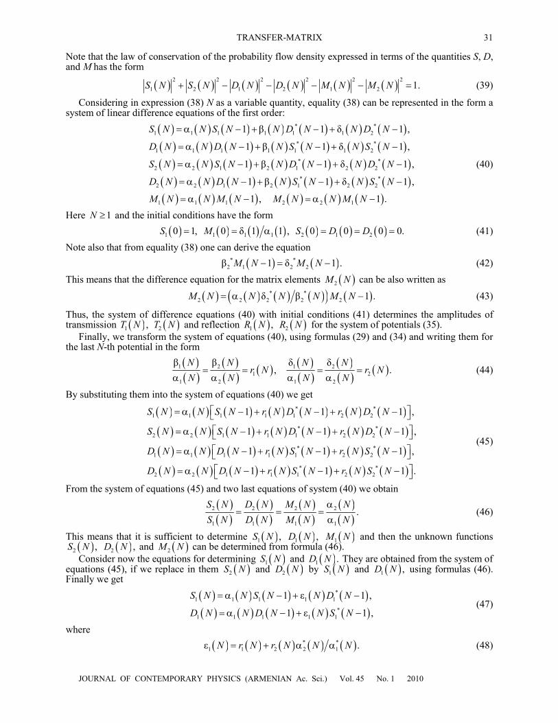
Note that the law of conservation of the probability flow density expressed in terms of the quantities S, D, and M has the form

2 2 2 2 2 2

1 2 1 2 1 2 1.S N S N D N D N M N M N (39)

Considering in expression (38) N as a variable quantity, equality (38) can be represented in the form a system of linear difference equations of the first order:

* *1 1 1 1 1 1 2

* *1 1 1 1 1 1 2

* *2 2 1 2 1 2 2

* *2 2 1 2 1 2 2

1 1 1 2 2 1

1 β 1 δ 1 ,

1 β 1 δ 1 ,

1 β 1 δ 1 ,

1 β 1 δ 1 ,

1 , 1 .

S N N S N N D N N D N

D N N D N N S N N S N

S N N S N N D N N D N

D N N D N N S N N S N

M N N M N M N N M N

(40)

Here 1N and the initial conditions have the form

1 1 1 1 2 1 20 1, 0 δ 1 1 , 0 0 0 0.S M S D D (41)

Note also that from equality (38) one can derive the equation

* *2 1 2 2β 1 δ 1 .M N M N (42)

This means that the difference equation for the matrix elements 2M N can be also written as

* *2 2 2 2 2δ β 1 .M N N N N M N (43)

Thus, the system of difference equations (40) with initial conditions (41) determines the amplitudes of transmission 1 ,T N 2T N and reflection 1 ,R N 2R N for the system of potentials (35).

Finally, we transform the system of equations (40), using formulas (29) and (34) and writing them for the last N-th potential in the form

1 2 1 2

1 21 2 1 2

β β δ δ, .

N N N Nr N r N

N N N N

(44)

By substituting them into the system of equations (40) we get

* *1 1 1 1 1 2 2

* *2 2 1 1 1 2 2

* *1 1 1 1 1 2 2

* *2 2 1 1 1 2 2

1 1 1 ,

1 1 1 ,

1 1 1 ,

1 1 1 .

S N N S N r N D N r N D N

S N N S N r N D N r N D N

D N N D N r N S N r N S N

D N N D N r N S N r N S N

(45)

From the system of equations (45) and two last equations of system (40) we obtain

2 2 2 2

1 1 1 1

.S N D N M N N

S N D N M N N

(46)

This means that it is sufficient to determine 1 ,S N 1 ,D N 1M N and then the unknown functions 2 ,S N 2 ,D N and 2M N can be determined from formula (46). Consider now the equations for determining 1S N and 1 .D N They are obtained from the system of

equations (45), if we replace in them 2S N and 2D N by 1S N and 1 ,D N using formulas (46). Finally we get

*1 1 1 1 1

*1 1 1 1 1

1 ε 1 ,

1 ε 1 ,

S N N S N N D N

D N N D N N S N

(47)

where

* *1 1 2 2 1ε .N r N r N N N (48)

SEDRAKIAN

32


The unknown function 1M N is determined from the equation

1 1 1 1 ,M N N M N (49)

which enters the system of equations (40). Note that the system of equations (47) coincides with the system of equations derived for the one-

dimensional scattering problem, but the coefficients before the functions 1 1S N and 1 1D N are other. Note also that the solution of such a system of equations was studied in [3, 5].

REFERENCES 1. Boese, D., Lischka, M., and Reichl, L.E., Phys. Rev. B, 2000, vol. 82, p. 16933. 2. Sedrakian, D.M., Kazaryan, E.M., and Sedrakian, L.R., J. Contemp. Phys. (Armenian Ac. Sci.), 2009, vol. 44,

p. 257. 3. Sedrakian, D.M. and Khachatrian, A.Zh., Doklady NAN Armenii, 1998, vol. 98, p. 301. 4. Sedrakian, D.M., Kazaryan, E.M., Sedrakian, L.R., and Khachatrian, A.Zh., J. Contemp. Phys. (Armenian Ac.

Sci.), 2009, vol. 44, p. 113. 5. Sedrakian, D.M., Badalyan, D.A., and Khachatrian, A.Zh., FTT, 1999, vol. 41, p. 1687. 6. Khachatrian, A.Zh., Sedrakian, D.M., and Khoetsyan, V.A., J. Contemp. Phys. (Armenian Ac. Sci.), 2009,

vol. 44, p. 91.

Documents

Transfer-matrix for the two-channel scattering problem