3D Kinematics

So now we’re pretty good at 2D kinematics, and we can expand this to 3D kinematics.

Transformation Matrices

The derivation of these follows the derivation of the 2D transformation matrices closely; you can grind yourway through the math on your own if you’d like. Since we’re in 3D, and since we’ll still need heterogeneous

matrices to perform translation, our points will now be represented with a 4× 1 vector

xyz1

, and our

transformation matrices will have to be 4× 4.

Translation

Trans(px, py, pz) =

1 0 0 px0 1 0 py0 0 1 pz0 0 0 1

Rotation around the X axis

RotX(φ) =

1 0 0 00 cos(φ) − sin(φ) 00 sin(φ) cos(φ) 00 0 0 1

Rotation around the Y axis

RotY(φ) =

cos(φ) 0 sin(φ) 0

0 1 0 0− sin(φ) 0 cos(φ) 0

0 0 0 1

Rotation around the Z axis

RotZ(φ) =

cos(φ) − sin(φ) 0 0sin(φ) cos(φ) 0 0

0 0 1 00 0 0 1

3D Coordinate Frames

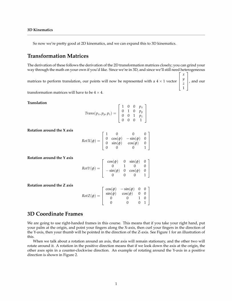
We are going to use right-handed frames in this course. This means that if you take your right hand, putyour palm at the origin, and point your fingers along the X-axis, then curl your fingers in the direction ofthe Y-axis, then your thumb will be pointed in the direction of the Z-axis. See Figure 1 for an illustration ofthis.

When we talk about a rotation around an axis, that axis will remain stationary, and the other two willrotate around it. A rotation in the positive direction means that if we look down the axis at the origin, theother axes spin in a counter-clockwise direction. An example of rotating around the Y-axis in a positivedirection is shown in Figure 2.

1

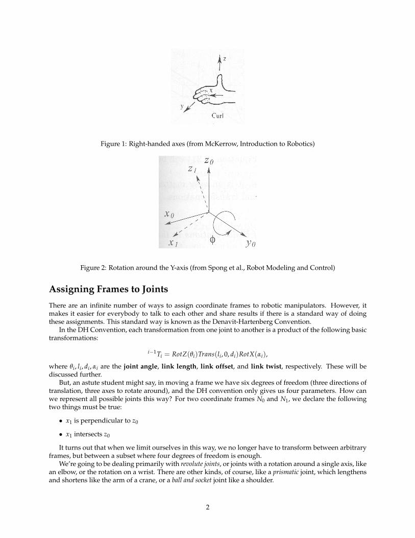
Figure 1: Right-handed axes (from McKerrow, Introduction to Robotics)

Figure 2: Rotation around the Y-axis (from Spong et al., Robot Modeling and Control)

Assigning Frames to Joints

There are an infinite number of ways to assign coordinate frames to robotic manipulators. However, itmakes it easier for everybody to talk to each other and share results if there is a standard way of doingthese assignments. This standard way is known as the Denavit-Hartenberg Convention.

In the DH Convention, each transformation from one joint to another is a product of the following basictransformations:

i−1Ti = RotZ(θi)Trans(li, 0, di)RotX(αi),

where θi, li, di, αi are the joint angle, link length, link offset, and link twist, respectively. These will bediscussed further.

But, an astute student might say, in moving a frame we have six degrees of freedom (three directions oftranslation, three axes to rotate around), and the DH convention only gives us four parameters. How canwe represent all possible joints this way? For two coordinate frames N0 and N1, we declare the followingtwo things must be true:

• x1 is perpendicular to z0

• x1 intersects z0

It turns out that when we limit ourselves in this way, we no longer have to transform between arbitraryframes, but between a subset where four degrees of freedom is enough.

We’re going to be dealing primarily with revolute joints, or joints with a rotation around a single axis, likean elbow, or the rotation on a wrist. There are other kinds, of course, like a prismatic joint, which lengthensand shortens like the arm of a crane, or a ball and socket joint like a shoulder.

2

On revolute joints, we will add the additional constraint on our frames that the joint will rotate aroundthe Z-axis.

Revolute joints which meet the above criteria can be broken down into the following three cases.

1. zi−1 and zi are parallel

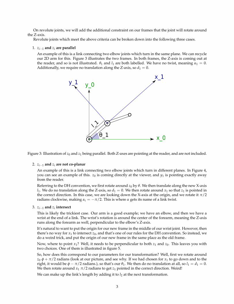
An example of this is a link connecting two elbow joints which turn in the same plane. We can recycleour 2D arm for this. Figure 3 illustrates the two frames. In both frames, the Z-axis is coming out atthe reader, and so is not illustrated. θ1 and l1 are both labelled. We have no twist, meaning α1 = 0.Additionally, we require no translation along the Z-axis, so d1 = 0.

x_0

y_0x_1

y_1

l_1

θ_1

Figure 3: Illustration of z0 and z1 being parallel. Both Z-axes are pointing at the reader, and are not included.

2. zi−1 and zi are not co-planar

An example of this is a link connecting two elbow joints which turn in different planes. In Figure 4,you can see an example of this. z0 is coming directly at the viewer, and y1 is pointing exactly awayfrom the reader.

Referring to the DH convention, we first rotate around z0 by θ. We then translate along the new X-axisl1. We do no translation along the Z-axis, so d1 = 0. We then rotate around x1 so that z1 is pointed inthe correct direction. In this case, we are looking down the X-axis at the origin, and we rotate it π/2radians clockwise, making αi = −π/2. This is where α gets its name of a link twist.

3. zi−1 and zi intersect

This is likely the trickiest case. Our arm is a good example; we have an elbow, and then we have awrist at the end of a link. The wrist’s rotation is around the center of the forearm, meaning the Z-axisruns along the forearm as well, perpendicular to the elbow’s Z-axis.

It’s natural to want to put the origin for our new frame in the middle of our wrist joint. However, thenthere’s no way for x1 to intersect z0, and that’s one of our rules for the DH convention. So instead, wedo a weird trick, and put the origin of our new frame in the same place as the old frame.

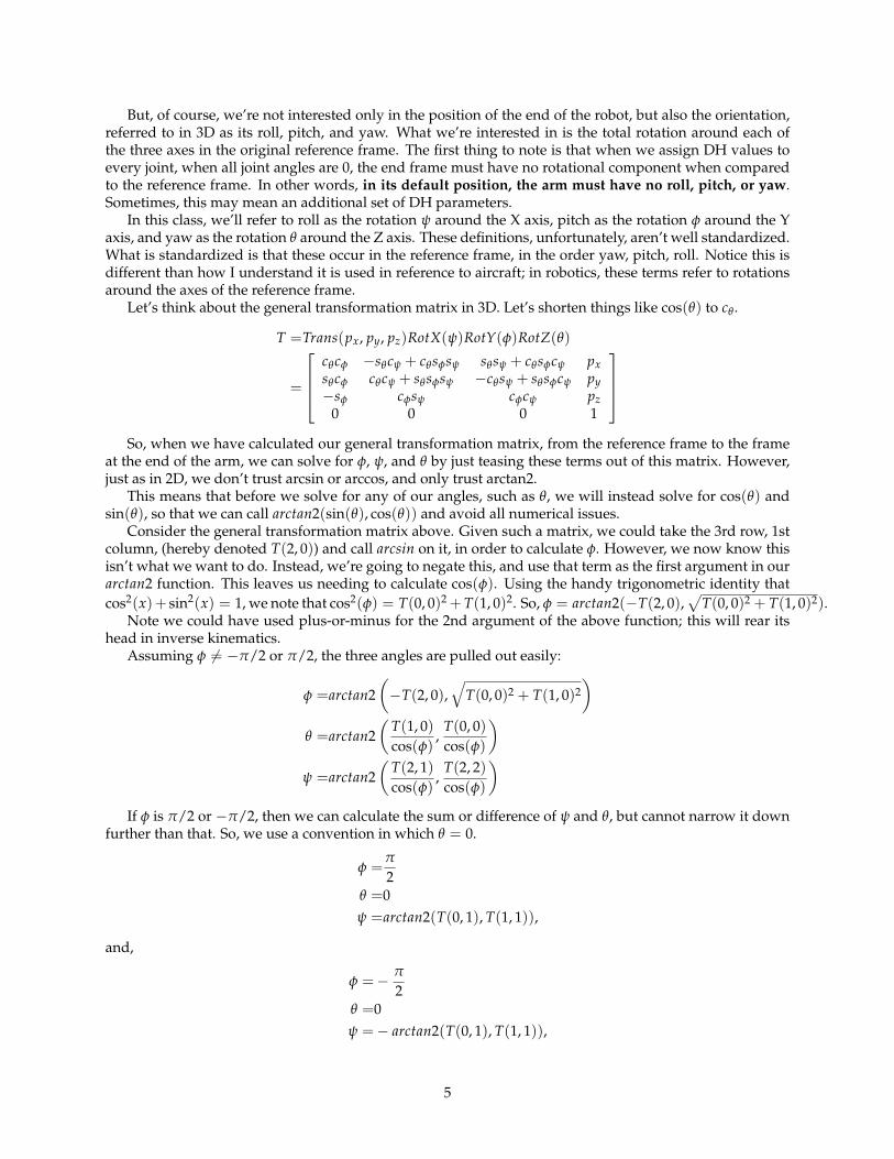
Now, where to point x1? Well, it needs to be perpendicular to both z1 and z0. This leaves you withtwo choices. One of them is illustrated in figure 5.

So, how does this correspond to our parameters for our transformation? Well, first we rotate aroundz0 φ + π/2 radians (look at our picture, and see why. If we had chosen for x1 to go down and to theright, it would be φ− π/2 radians.), so that’s our θ1. We then do no translation at all, so l1 = d1 = 0.We then rotate around x1 π/2 radians to get z1 pointed in the correct direction. Weird!

We can make up the link’s length by adding it to l2 at the next transformation.

3

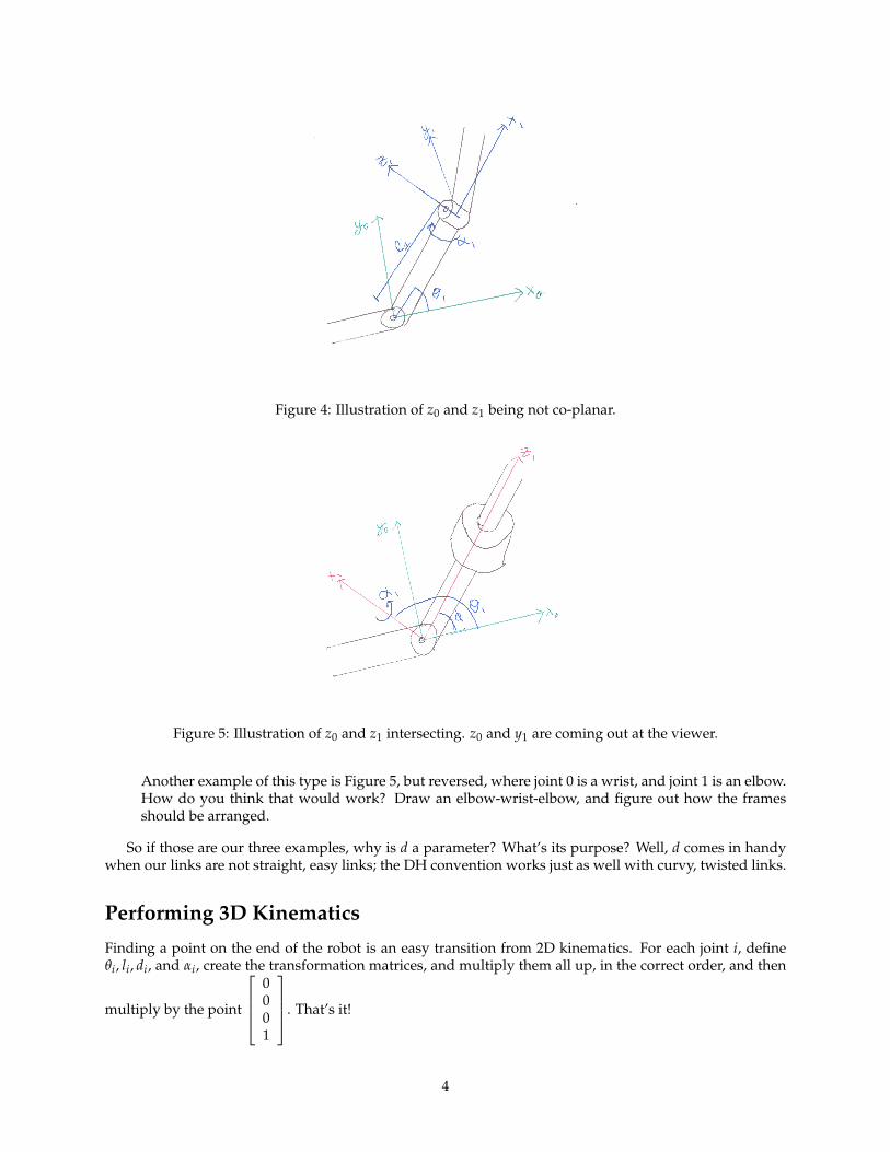
Figure 4: Illustration of z0 and z1 being not co-planar.

Figure 5: Illustration of z0 and z1 intersecting. z0 and y1 are coming out at the viewer.

Another example of this type is Figure 5, but reversed, where joint 0 is a wrist, and joint 1 is an elbow.How do you think that would work? Draw an elbow-wrist-elbow, and figure out how the framesshould be arranged.

So if those are our three examples, why is d a parameter? What’s its purpose? Well, d comes in handywhen our links are not straight, easy links; the DH convention works just as well with curvy, twisted links.

Performing 3D Kinematics

Finding a point on the end of the robot is an easy transition from 2D kinematics. For each joint i, defineθi, li, di, and αi, create the transformation matrices, and multiply them all up, in the correct order, and then

multiply by the point

0001

. That’s it!

4

But, of course, we’re not interested only in the position of the end of the robot, but also the orientation,referred to in 3D as its roll, pitch, and yaw. What we’re interested in is the total rotation around each ofthe three axes in the original reference frame. The first thing to note is that when we assign DH values toevery joint, when all joint angles are 0, the end frame must have no rotational component when comparedto the reference frame. In other words, in its default position, the arm must have no roll, pitch, or yaw.Sometimes, this may mean an additional set of DH parameters.

In this class, we’ll refer to roll as the rotation ψ around the X axis, pitch as the rotation φ around the Yaxis, and yaw as the rotation θ around the Z axis. These definitions, unfortunately, aren’t well standardized.What is standardized is that these occur in the reference frame, in the order yaw, pitch, roll. Notice this isdifferent than how I understand it is used in reference to aircraft; in robotics, these terms refer to rotationsaround the axes of the reference frame.

Let’s think about the general transformation matrix in 3D. Let’s shorten things like cos(θ) to cθ .

T =Trans(px, py, pz)RotX(ψ)RotY(φ)RotZ(θ)

=

cθcφ −sθcψ + cθsφsψ sθsψ + cθsφcψ pxsθcφ cθcψ + sθsφsψ −cθsψ + sθsφcψ py−sφ cφsψ cφcψ pz

0 0 0 1

So, when we have calculated our general transformation matrix, from the reference frame to the frame

at the end of the arm, we can solve for φ, ψ, and θ by just teasing these terms out of this matrix. However,just as in 2D, we don’t trust arcsin or arccos, and only trust arctan2.

This means that before we solve for any of our angles, such as θ, we will instead solve for cos(θ) andsin(θ), so that we can call arctan2(sin(θ), cos(θ)) and avoid all numerical issues.

Consider the general transformation matrix above. Given such a matrix, we could take the 3rd row, 1stcolumn, (hereby denoted T(2, 0)) and call arcsin on it, in order to calculate φ. However, we now know thisisn’t what we want to do. Instead, we’re going to negate this, and use that term as the first argument in ourarctan2 function. This leaves us needing to calculate cos(φ). Using the handy trigonometric identity thatcos2(x)+ sin2(x) = 1, we note that cos2(φ) = T(0, 0)2 +T(1, 0)2. So, φ = arctan2(−T(2, 0),

√T(0, 0)2 + T(1, 0)2).

Note we could have used plus-or-minus for the 2nd argument of the above function; this will rear itshead in inverse kinematics.

Assuming φ 6= −π/2 or π/2, the three angles are pulled out easily:

φ =arctan2(−T(2, 0),

√T(0, 0)2 + T(1, 0)2

)θ =arctan2

(T(1, 0)cos(φ)

,T(0, 0)cos(φ)

)ψ =arctan2

(T(2, 1)cos(φ)

,T(2, 2)cos(φ)

)If φ is π/2 or −π/2, then we can calculate the sum or difference of ψ and θ, but cannot narrow it down

further than that. So, we use a convention in which θ = 0.

φ =π

2θ =0ψ =arctan2(T(0, 1), T(1, 1)),

and,

φ =− π

2θ =0ψ =− arctan2(T(0, 1), T(1, 1)),

5