Embed Size (px)
Citation preview

TRANSFORMER AC WINDING RESISTANCE AND DERATING WHEN SUPPLYING HARMONIC-RICH
CURRENT
By
Jian Zheng
A Thesis
Submitted in partial fulfillment of the requirements
for the degree of
MASTER OF SCIENCE IN ELECTRICAL ENGINEERING
Michigan Technological University
2000

i
ABSTRACT
Transformer loading with harmonic-rich current and subsequent overheating is an
ongoing concern of electric utilities and consumers. UL Standards 1561 and 1562 suggest
using a K-factor for determination of transformer capacity with nonlinear loads.
This work focuses at investigating the concept of K-factor and the relationship be-
tween K-factor, transformer derating, and the transformer winding eddy-current loss.
The relationship between K-factor and AC winding resistance is investigated. Laboratory
test procedures for measuring the AC winding resistance of two type of distribution trans-
formers are developed and explained. Test procedures for checking the linearity and su-
perposition assumptions are also developed.
From the test results, it is found that linearity and superposition holds very well
for the test transformers while the K-factor overestimates the losses in transformer wind-
ings. The difference between K-factor results and lab test results is explained. Another
approach for estimating the total stray loss in transformer winding, the Harmonic Loss
Factor, is discussed and found to be a better solution.

ii
ACKNOWLEDGEMENTS
I would like to express my sincere gratitude to my advisor, Dr. Leo-
nard Bohmann, for his insights and direction through this research. He has
been an excellent advisor, patient, and helpful all through the time.
I take this opportunity to thank Dr. Bruce Mork, for his help and sug-
gestions during the course of the research.
Special thanks to my committee members: Dr. Noel Schulz and Dr.
Konrad Heuvers for their time spent on reviewing this work. Their insights
and suggestions are greatly appreciated.
Besides the professors I have listed, I would also like to thank all of
the faculty and staff of the Electrical Engineering Department, especially
Scott Ackerman, John Miller, and Chuck Sannes, for being so helpful.
Finally, I wish to thank my family and friends for all the support they
have provided. Your support made my stay at Michigan Tech one that I will
never forget and always cherish.

iii
TABLE OF CONTENTS ABSTRACT………………………………………………………………………………i ACKNOWLEDGEMENTS………………………………………………………………ii TABLE OF CONTENTS...………………………………………………………………iii LIST OF FIGURES AND TABLES …..…………………………………………………v CHAPTER 1 INTRODUCTION................................................................................................................. 1
CHAPTER 2 INTRODUCTION TO TEST TRANSFORMER AND K-FACTOR............................... 4
2.1 SINGLE PHASE TRANSFORMER MODEL................................................................................................. 4 2.2 THE TEST TRANSFORMERS.................................................................................................................... 5 2.3 TRANSFORMER LOSSES AND THE AC WINDING RESISTANCE............................................................... 7 2.4 K-FACTOR ............................................................................................................................................ 9 2.5 HARMONIC LOSS FACTOR................................................................................................................... 12
CHAPTER 3 LABORATORY TESTS..................................................................................................... 14
3.1 MEASUREMENT CONSIDERATION ....................................................................................................... 14 3.2 TEST DEVICES..................................................................................................................................... 15
3.2.1 Power source ............................................................................................................................. 15 3.2.2 UPC-32 ...................................................................................................................................... 16 3.2.3 Oscilloscope............................................................................................................................... 17
3.3 SHORT-CIRCUIT TESTS......................................................................................................................... 17 3.3.1 2KVA distribution Transformer ................................................................................................ 17 3.3.2 10 KVA distribution Transformer .............................................................................................. 18 3.3.3 Data Recording.......................................................................................................................... 18
3.4 HARMONIC TEST ................................................................................................................................. 19 3.5 DATA SAMPLING AND DFT ................................................................................................................ 19 3.6. SPECIAL CONSIDERATION IN THE TESTS ............................................................................................. 22
CHAPTER 4 TEST RESULTS AND ANALYSIS................................................................................... 23
4.1 LINEARITY .......................................................................................................................................... 23 4.2 SUPERPOSITION................................................................................................................................... 24 4.3 TEMPERATURE VARIATIONS ............................................................................................................... 25 4.4 SHORT CIRCUIT TEST RESULTS .......................................................................................................... 26
4.4.1 10 KVA distribution transformer ............................................................................................... 26 4.4.2 2 KVA distribution transformer ................................................................................................. 32
4.5 TEST RESULTS ANALYSIS .................................................................................................................... 38
CHAPTER 5 CONCLUSIONS AND RECOMMENDATION ............................................................. 41
5.1 CONCLUSIONS................................................................................................................................ 41 5.2 RECOMMENDATIONS FOR FUTURE WORK............................................................................................ 42
REFERENCE: ............................................................................................................................................ 43
APPENDIX A 10 KVA DISTRIBUTION XFMR SHORT CIRCUIT TEST RESULTS .................... 46
APPENDIX B 2 KVA DISTRIBUTION TRANSFORMER SHORT CIRCUIT TEST RESULTS ... 50
APPENDIX C HARMONIC GROUP TEST RESULTS........................................................................ 54

iv
APPENDIX D MATLAB PROGRAM FOR ANALYSIS OF 2 KVA TRANSFORMER SHORT CIRCUIT TEST RESULTS ...................................................................................................................... 55
APPENDIX E MATLAB PROGRAM FOR ANALYSIS OF 10 KVA TRANSFORMER SHORT CIRCUIT TEST RESULTS ...................................................................................................................... 60
APPENDIX F INSTRUCTIONS FOR DOING SHORT CIRCUIT TEST MANUALLY .................. 66
APPENDIX G LABORATORY EQUIPMENT AND COMPUTER RESOURCES ........................... 67
v
LIST OF FIGURES AND TABLES FIGURE 2-1 CORE AND SHELL FORMS WITH WINDINGS................................................................................... 4 FIGURE 2-2 SIMPLIFIED SINGLE-PHASE TRANSFORMER MODEL ..................................................................... 5 FIGURE 2-3 FOUR WINDING CORE-SECTION WITH MAIN LEAKAGE PATHS SHOWN........................................ 5 FIGURE 2-4 10KVA, AMORPHOUS STEEL CORE SINGLE-PHASE DISTRIBUTION TRANSFORMER ........................ 6 FIGURE 2-5 WINDING EDDY-CURRENT INDUCED BY MAGNETIC FLUX IN THE WINDING CONDUCTORS............. 8 FIGURE 3-1. LABORATORY SETUP FOR SHORT-CIRCUIT TESTS ON 2 KVA DISTRIBUTION XFMR................ 17 FIGURE 3-2. LAB SETUP FOR SHORT-CIRCUIT TESTS OF THE 10 KVA DISTRIBUTION XFMR....................... 18 FIGURE 3-3. LINE SPECTRUM......................................................................................................................... 21 TABLE 3-1TIME STEP VALUES AND CORRESPONDING DFT FREQUENCY SPACINGS FOR DIFFERENT NUMBERS
OF POINTS TRANSFORMED. ................................................................................................................... 20 FIGURE 4-1 TEMPERATURE EFFECT ON THE WINDING RESISTANCE ............................................................... 25 FIGURE 4-2 SHORT-CIRCUIT TEST RESULTS: R.X VS. FREQUENCY (10KVA TRANSFORMER) ...................... 27 FIGURE 4-3 2ND FIT FOR RAC (FH/F1)2 FROM 60 HZ TO 2940 HZ (25 POINTS)............................................... 28 FIGURE 4-4 OPTIMAL FIT FOR 10 KVA RAC FROM 60 - 2940 HZ ( ALL THE 25 POINTS) ............................... 29 FIGURE 4-5 TOTAL FIT ERROR WHILE TRANSITION POINT MOVES. (SQUARE/NON-SQUARE) .......................... 30 FIGURE 4-6 TOTAL FIT ERROR WHILE TRANSITION POINT MOVES (BOTH SECTIONS ARE OPTIMAL FIT) .......... 31 FIGURE 4-7 2KVA XFMR AC WINDING RESISTANCE (AUTOMATIC TEST RESULTS).................................... 33 FIGURE 4-8 ONE SECTION FIT FOR 2KVA XFMR AC WINDING RESISTANCE DATA .................................... 34 FIGURE 4-9 ONE SECTION OPTIMAL FIT FOR 2 KVA XFMR RAC (60-1680 HZ)........................................... 35 FIGURE 4-10 THE TOTAL FITTING ERROR WHILE THE TRANSITION POINTS BETWEEN 2ND ORDER FIT AND
OPTIMAL FIT MOVES............................................................................................................................. 36 FIGURE 4-11 THE TOTAL FITTING ERROR WHILE THE TRANSITION POINTS BETWEEN TWO OPTIMAL FIT
REGIMES MOVES .................................................................................................................................. 37 TABLE 4-1 LINEARITY CHECK ON 10 KVA TRANSFORMER........................................................................... 23 TABLE 4-2 SUPERPOSITION CHECK RESULTS ................................................................................................ 24 TABLE 4-3 MEASURED AC WINDING RESISTANCE AND REACTANCE AT DIFFERENT FREQUENCIES. .............. 26 TABLE 4-4 FITTING METHODS COMPARISON FOR 10 KVA TRANSFORMER DATA.......................................... 32 TABLE 4-5 MEASURED 2 KVA TRANSFORMER AC WINDING RESISTANCE ................................................... 32 TABLE 4-6 FITTING METHODS COMPARISON FOR 2 KVA TRANSFORMER DATA............................................ 38 TABLE A-1 10 KVA DISTRIBUTION TRANSFORMER TEST NO.1 ................................................................... 46 TABLE A-2 10 KVA DISTRIBUTION TRANSFORMER TEST NO.2.................................................................... 47 TABLE A-3 10 KVA DISTRIBUTION TRANSFORMER TEST NO.3.................................................................... 48 TABLE A-4 10 KVA DISTRIBUTION TRANSFORMER RDC TEST RESULTS...................................................... 49 TABLE B-1 2 KVA MANUAL SHORT CIRCUIT TEST RESULTS....................................................................... 50 TABLE B-2 2 KVA AUTOMATIC SHORT CIRCUIT TEST RESULTS [18] .......................................................... 51 TABLE B-3 2 KVA DC VALUE TEST RESULTS ............................................................................................. 53 TABLE C-1 2 KVA DISTRIBUTION TRANSFORMER HARMONIC GROUP TEST RESULTS 1.............................. 54 TABLE C-2 KVA DISTRIBUTION TRANSFORMER HARMONIC GROUP TEST RESULTS 2................................. 54 TABLE C-3 DFT ACCURACY CHECK (10 KVA TRANSFORMER)................................................................... 54

1
________________________________________________
CHAPTER 1
INTRODUCTION
________________________________________________
With the ever-increasing use of solid state electronics in electrical load devices,
such as switching power supplies, variable-speed drives and many types of office
equipment [6], the power system network is being subjected to higher levels of harmonic
currents. One result of this trend is excessive internal heating in power distribution
transformers that are loaded with harmonic-rich current.
The transformer manufacturers have improved their design in response to these
heating problems. Design changes include enlarging the primary winding to withstand the
inherent triplen harmonic circulating currents, doubling the secondary neutral conductor
to carry the triplen1 harmonic currents, designing the magnetic core with a lower normal
flux density by using higher grades of iron, and using smaller, insulated secondary
conductors wired in parallel and transposed to reduce the heating from the skin effect and
associated AC resistance.
Several methods of estimating the harmonic load content are available. Crest-
Factor and Percent Total Harmonic Distortion (%THD) are the two common methods.
1 Triplen harmonics are created by non-linear loads. They flow in the neutral conductor and windings of the power transformer. They are odd harmonics devisable by three, including the 3rd, 9th, 15th, and 21st.
2
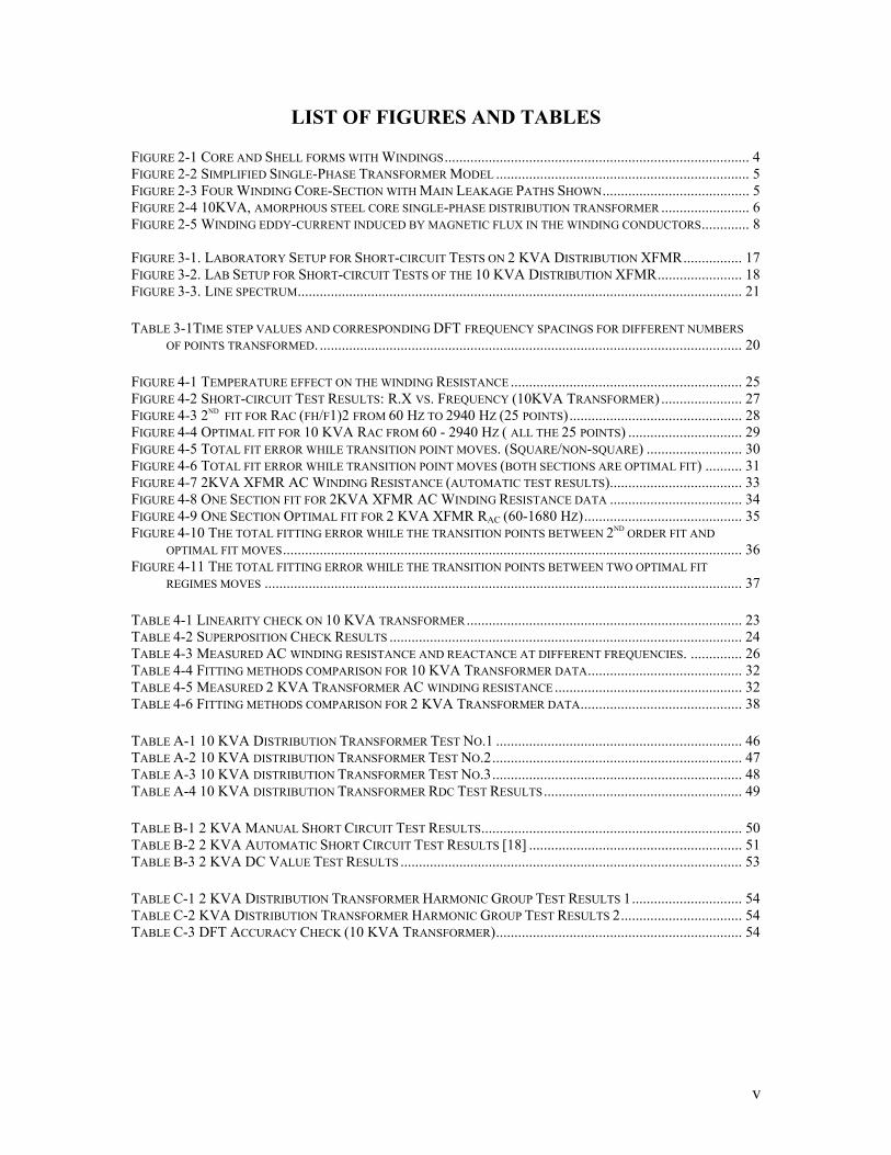
The third method “K-Factor” can be used to estimate the additional heat created by non-
sinusoidal loads
The crest factor is a measure of the peak value of the waveform compared to the
true RMS value
currenttheofRMSTrueWaveformCurrenttheofMagnitudePeakFactorCrest =−
(1.1)
The %THD is a ratio of the root-mean-square (RMS) value of the harmonic
current to the RMS value of the fundamental.
1
2
2)(%
I
ITHD h
h∑∞
== (1.2)
It is a measure of the additional harmonic current contribution to the total RMS
current.
Both of the above methods are limited because frequency characteristics of the
transformer are not considered.
The third method, K-factor, is defined as the sum of the squares of the per unit
harmonic current times the harmonic number squared:
∑∞
=
=1
22)( )(
hpuh hIK
(1.3)
where Ih(pu) is the harmonic current expressed in per unit based upon the
magnitude of the fundamental current and h is the harmonic number.

3
K-factor was introduced in UL standards 1561 [14] and 1562 [15] for rating
transformers based on their capability to handle load currents with significant harmonic
content.
Field application of K-factor requires knowledge of the fundamental and
harmonic load current magnitudes expected. Several manufacturers have utilized this
standard to market transformers that are specifically designed to carry the additional
harmonic currents.
This thesis is aimed at investigating the concept of K-factor and the relationship
between K-factor, derating, and the winding eddy-current loss of harmonic currents.
Chapter 2 presents the structure of the transformer under study, the K-factor theory and
existing work. Chapter 3 documents the test procedure and data processing methods
developed for determining the winding eddy-current loss, AC winding resistance and K-
factor. Chapter 4 compares the results of the measurements with the ideal results of the
K-factor theory and explains the difference. Chapter 5 provides conclusions and
recommendations for further research.
4
________________________________________________
CHAPTER 2
INTRODUCTION TO TEST TRANSFORMER AND K-FACTOR ________________________________________________
This chapter includes a general discussion of the single-phase transformer, a
description of the test transformers and the definition of the K-factor.
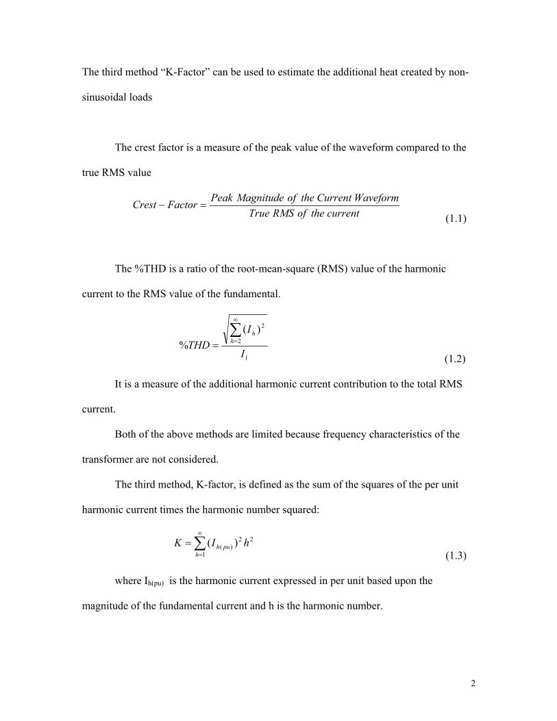
2.1 SINGLE PHASE TRANSFORMER MODEL.
There are two basic core designs for single-phase transformer: core form and shell
form.
a) Core b) Shell
Figure 2-1 Core and Shell forms with Windings
Due to insulation requirements, the low voltage (LV) winding normally appears
closest to the core, while the high voltage (HV) winding appears outside. The windings
are usually referred to as primary and secondary winding(s) as denoted by the P and S. In
the shell form, the flux generated in the core by the windings splits equally in both "legs"
of the core. Winding configurations may vary with core design and include concentric
φφ/2
5
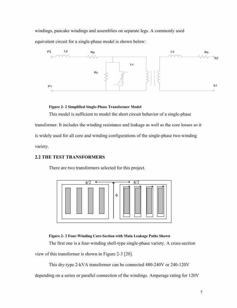
windings, pancake windings and assemblies on separate legs. A commonly used
equivalent circuit for a single-phase model is shown below:
P2
P1
Lp Rp
Rc
Lc
Ls Rs
S2
S1
Figure 2- 2 Simplified Single-Phase Transformer Model
This model is sufficient to model the short circuit behavior of a single-phase
transformer. It includes the winding resistance and leakage as well as the core losses so it
is widely used for all core and winding configurations of the single-phase two-winding
variety.
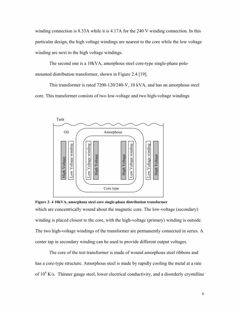
2.2 THE TEST TRANSFORMERS
There are two transformers selected for this project.
φ/2
φ
φ/2
Figure 2- 3 Four-Winding Core-Section with Main Leakage Paths Shown
The first one is a four-winding shell-type single-phase variety. A cross-section
view of this transformer is shown in Figure 2-3 [20].
This dry-type 2-kVA transformer can be connected 480-240V or 240-120V
depending on a series or parallel connection of the windings. Amperage rating for 120V
6
winding connection is 8.33A while it is 4.17A for the 240 V winding connection. In this
particular design, the high voltage windings are nearest to the core while the low voltage
winding are next to the high voltage windings.
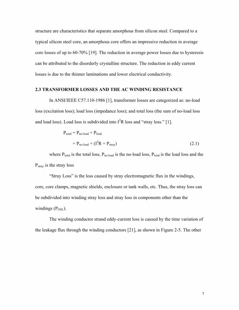
The second one is a 10kVA, amorphous steel core-type single-phase pole-
mounted distribution transformer, shown in Figure 2.4 [19].
This transformer is rated 7200-120/240-V, 10 kVA, and has an amorphous steel
core. This transformer consists of two low-voltage and two high-voltage windings
Figure 2- 4 10kVA, amorphous steel core single-phase distribution transformer
which are concentrically wound about the magnetic core. The low-voltage (secondary)
winding is placed closest to the core, with the high-voltage (primary) winding is outside.
The two high-voltage windings of the transformer are permanently connected in series. A
center tap in secondary winding can be used to provide different output voltages.
The core of the test transformer is made of wound amorphous steel ribbons and
has a core-type structure. Amorphous steel is made by rapidly cooling the metal at a rate
of 106 K/s. Thinner gauge steel, lower electrical conductivity, and a disorderly crystalline
Core type
Amorphous
Hig
h V
olta
ge
Low
Vol
tage
win
ding
Hig
h V
olta
ge
Hig
h V
olta
ge
Hig
h V
olta
ge
Low
Vol
tage
win
ding
Low
Vol
tage
win
ding
Low
Vol
tage
win
ding
Tank
Oil
7
structure are characteristics that separate amorphous from silicon steel. Compared to a
typical silicon steel core, an amorphous core offers an impressive reduction in average
core losses of up to 60-70% [19]. The reduction in average power losses due to hysteresis
can be attributed to the disorderly crystalline structure. The reduction in eddy current
losses is due to the thinner laminations and lower electrical conductivity.
2.3 TRANSFORMER LOSSES AND THE AC WINDING RESISTANCE
In ANSI/IEEE C57.110-1986 [1], transformer losses are categorized as: no-load
loss (excitation loss); load loss (impedance loss); and total loss (the sum of no-load loss
and load loss). Load loss is subdivided into I2R loss and “stray loss.” [1].
Ptotal = Pno-load + Pload
= Pno-load + (I2R + Pstray) (2.1)
where Ptotal is the total loss, Pno-load is the no-load loss, Pload is the load loss and the
Pstray is the stray loss
“Stray Loss” is the loss caused by stray electromagnetic flux in the windings,
core, core clamps, magnetic shields, enclosure or tank walls, etc. Thus, the stray loss can
be subdivided into winding stray loss and stray loss in components other than the
windings (POSL).
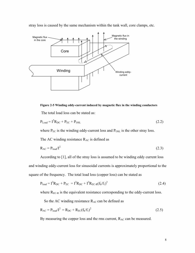
The winding conductor strand eddy-current loss is caused by the time variation of
the leakage flux through the winding conductors [21], as shown in Figure 2-5. The other
8
stray loss is caused by the same mechanism within the tank wall, core clamps, etc.
Magnetic fluxin the core
Magnetic flux inthe winding
Winding eddy-current
Core
Winding
Figure 2-5 Winding eddy-current induced by magnetic flux in the winding conductors
The total load loss can be stated as:
PLoad = I2RDC + PEC + POSL (2.2)
where PEC is the winding eddy-current loss and POSL is the other stray loss.
The AC winding resistance RAC is defined as
RAC = Pload/I2 (2.3)
According to [1], all of the stray loss is assumed to be winding eddy current loss
and winding eddy-current loss for sinusoidal currents is approximately proportional to the
square of the frequency. The total load loss (copper loss) can be stated as
Pload = I2RDC + PEC = I2RDC + I2REC-R(fh/f1)2 (2.4)
where REC-R is the equivalent resistance corresponding to the eddy-current loss.
So the AC winding resistance RAC can be defined as
RAC = Pload/I2 = RDC + REC(fh/f1)2 (2.5)
By measuring the copper loss and the rms current, RAC can be measured.
9
2.4 K-FACTOR
UL standards 1561 [14] and 1562 [15] introduced a term called the K-factor for
rating transformers based on their capability to handle load currents with significant
harmonic content. This method is based on the ANSI/IEEE C57.110-1986 standard,
Recommended Practice for Establishing Transformer Capability When Supplying
Nonsinusoidal Load Currents [1].
The K-factor is an estimate of the ratio of: (a) the heating in a transformer due to
winding eddy currents when it is loaded with a given nonsinusoidal current to (b) the
winding eddy-current heating caused by a sinusoidal current at the rated line frequency
which has the same RMS value as the nonsinusoidal current. For example, if the current
in a transformer winding is 100 A, and this current has a K-factor of 10, then the eddy
current losses in that winding will be approximately 10 times what they would be for a
100 A sinusoidal current at the rated line frequency.
Although the K-factor formula was defined for transformer currents, K-factors of
individual load currents are sometimes computed. This practice can be misleading
because, in general, K-factors measured at transformers are significantly lower than the
relatively high K-factors commonly measured at the input of individual electronic
devices. The reduction is primarily due to other sinusoidal load currents, power system
impedance and the essentially random phase angles of the harmonic currents produced by
various loads.
The AC loss in a transformer winding is mainly due to the sum of the I2R losses
produced by the fundamental and harmonic components of the current, recognizing that
for each component, R depends on the frequency of that component. For lower-order
10
harmonics, the frequency dependence of the winding resistance is primarily due to the
proximity effect, a phenomenon that occurs in coils because the magnetic field
surrounding each conductor in a coil depends on the fields produced by other conductors.
The proximity effect produces greater losses than those predicted by the skin effect,
which is dominant at higher frequencies [2].
The K-factor formula does not account for the core eddy current losses and other
losses that occur in transformer cores. Core losses due to harmonics depend primarily on
the voltage distortion across the transformer windings. The voltage distortion appearing
across the windings of a transformer carrying harmonic currents depends on the
impedance of the transformer, the impedance of the system feeding the transformer, and
the voltage distortion of that system. Although K-rated transformers are usually
constructed to withstand more voltage distortion than other transformers, this capability
cannot be directly determined from K ratings [2].
The K-factor formula is based on the assumption that the winding eddy current
loss produced by each harmonic component of a nonsinusoidal current is proportional to
the square of the harmonic order as well as being proportional to the square of the
magnitude of the harmonic component. UL defines K-factor as follows: [1]
(1) “K-FACTOR – A rating optionally applied to a transformer indicating its
suitability for use with loads that draw nonsinusoidal currents.”
(2) “The K-factor equals
∑∞
=
=1
22)( )(
hpuh hIK
(2.6)
where Ih(pu) is the rms current at harmonic “h” (per unit of rated rms load
current) and h is the harmonic order.”
11
(3) “K-factor rated transformers have not been evaluated for use with harmonic
loads where the rms current of any singular harmonic greater than the tenth
harmonic is greater than 1/h of the fundamental rms current.”
K-factor definition is based on the following two assumptions:
(a) Winding eddy-current loss (PEC) is proportional to the square of the load
current and the square of the frequency.
(b) Superposition of eddy current losses will apply, which will permit the direct
addition of eddy losses due to the various harmonics.
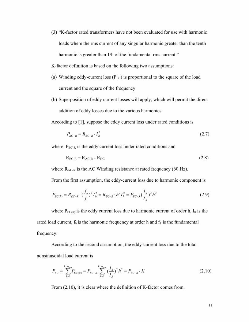
According to [1], suppose the eddy current loss under rated conditions is
2RRECREC IRP ⋅= −− (2.7)
where PEC-R is the eddy current loss under rated conditions and
REC-R = RAC-R - RDC (2.8)
where RAC-R is the AC Winding resistance at rated frequency (60 Hz).
From the first assumption, the eddy-current loss due to harmonic component is
222222
1)( )()( h
IIPIhRI
ffRP
R
hREChRECh
hREChEC −−− =⋅=⋅= (2.9)
where PEC(h) is the eddy current loss due to harmonic current of order h, IR is the
rated load current, fh is the harmonic frequency at order h and f1 is the fundamental
frequency.
According to the second assumption, the eddy-current loss due to the total
nonsinusoidal load current is
KPhIIPPP REC
hh
h R
hREC
hh
hhECEC ⋅=== −
=
=−
=
=∑∑
maxmax
1
22
1)( )( (2.10)
From (2.10), it is clear where the definition of K-factor comes from.
12
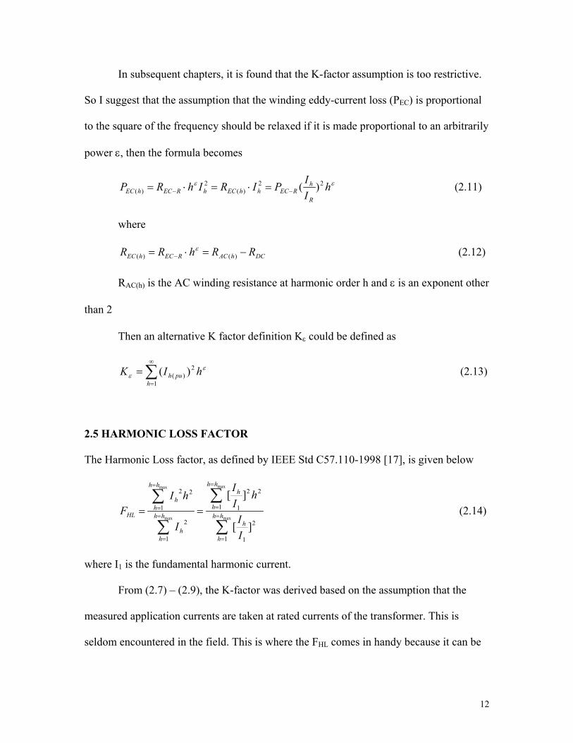
In subsequent chapters, it is found that the K-factor assumption is too restrictive.
So I suggest that the assumption that the winding eddy-current loss (PEC) is proportional
to the square of the frequency should be relaxed if it is made proportional to an arbitrarily
power ε, then the formula becomes
εε hIIPIRIhRP
R
hREChhEChREChEC
22)(
2)( )(−− =⋅=⋅= (2.11)
where
DChACREChEC RRhRR −=⋅= − )()(ε (2.12)
RAC(h) is the AC winding resistance at harmonic order h and ε is an exponent other
than 2
Then an alternative K factor definition Kε could be defined as
∑∞
=
=1
2)( )(
hpuh hIK ε
ε (2.13)
2.5 HARMONIC LOSS FACTOR
The Harmonic Loss factor, as defined by IEEE Std C57.110-1998 [17], is given below
∑
∑
∑
∑=
=
=
==
=
=
= ==max
max
max
max
1
2
1
1
22
1
1
2
1
22
][
][
hh
h
h
hh
h
h
hh
hh
hh
hh
HL
II
hII
I
hIF (2.14)
where I1 is the fundamental harmonic current.
From (2.7) – (2.9), the K-factor was derived based on the assumption that the
measured application currents are taken at rated currents of the transformer. This is
seldom encountered in the field. This is where the FHL comes in handy because it can be
13
calculated in terms of the actual rms values of the harmonic currents and the quantity Ih/I1
may be directly read on a meter.
The relationship between K-factor and FHL is
HLR
hh
hh
FI
IfactorK
=−∑=
=2
1
2max
(2.15)
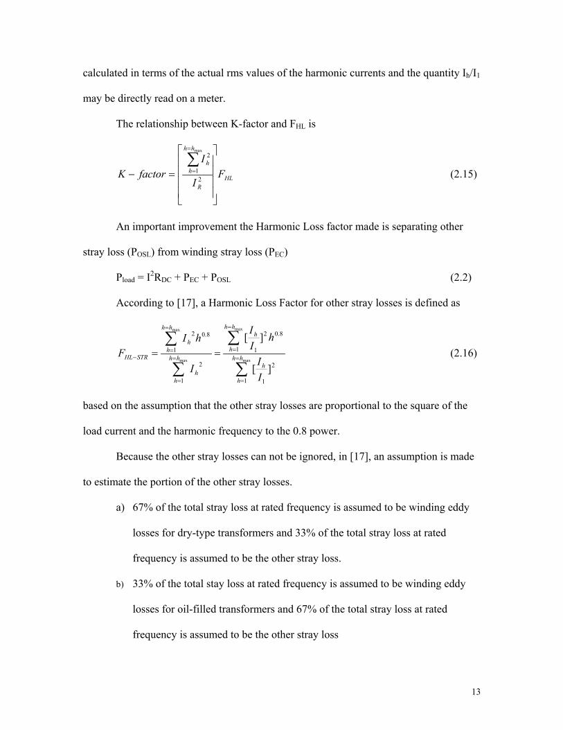
An important improvement the Harmonic Loss factor made is separating other
stray loss (POSL) from winding stray loss (PEC)
Pload = I2RDC + PEC + POSL (2.2)
According to [17], a Harmonic Loss Factor for other stray losses is defined as
∑
∑
∑
∑=
=
=
==
=
=
=− ==
max
max
max
max
1
2
1
1
8.02
1
1
2
1
8.02
][
][
hh
h
h
hh
h
h
hh
hh
hh
hh
STRHL
II
hII
I
hIF (2.16)
based on the assumption that the other stray losses are proportional to the square of the
load current and the harmonic frequency to the 0.8 power.
Because the other stray losses can not be ignored, in [17], an assumption is made
to estimate the portion of the other stray losses.
a) 67% of the total stray loss at rated frequency is assumed to be winding eddy
losses for dry-type transformers and 33% of the total stray loss at rated
frequency is assumed to be the other stray loss.
b) 33% of the total stay loss at rated frequency is assumed to be winding eddy
losses for oil-filled transformers and 67% of the total stray loss at rated
frequency is assumed to be the other stray loss
14
________________________________________________
CHAPTER 3
LABORATORY TESTS ________________________________________________
This chapter presents the test procedure and data processing methods developed
for determining the winding eddy-current loss, AC winding resistance and K-factor.
Detailed test procedure can be found in Appendix F and [18].
3.1 MEASUREMENT CONSIDERATION
The determination of parameters for transformer equivalent circuit models has
typically been based on meter measurements. Voltages and currents are measured with
RMS meters, and power is measured with an average reading wattmeter. Significant
measurement errors are possible for harmonic study. Only a “true RMS” meter can take
measurements which correctly include the effect of all harmonics within the meter’s
bandwidth. However the information about the harmonic content is lost.
In order to improve the accuracy of the measurement results, a digital storage
oscilloscope was used to record the waveforms of the voltage and current. A voltage
probe of ratio 1:100 was used. Hall effect current probe with a 1:1 ratio was used to
obtain current waveforms. The digital scope could save the sampled data on floppy
diskette. This allowed waveform data to be transported to a PC for analysis using the
VuPoint software, which was capable of many signal- processing operations.
15
3.2 TEST DEVICES 3.2.1 Power source
The power source used, AMX-3120, is a product of Pacific Power Source
Corporation (PPSC). It is a high-performance AC power conversion equipment. For our
test purposes, 3-phase voltage with programmable harmonic contents can be generated
from this device. It is configured with an interchangeable digital controller called the
Universal Programmable Controller (UPC). This programmable controller not only
allows control of voltage and frequency, but also allows the user to simulate virtually any
transient (including sub-cycle waveform disturbance). Main features of the power source
are: [11]
• Capable of 1, 2 or 3 phase operation
• Master Slave arrangement to obtain precise control
• Standard output range is 0-135 VAC(1-n )
• Phase separation fixed @ 180° for 2-phase operation
• Phase separation is programmable for 3-phase operation. Default is 120°
• Output power rating is 12 kVA
• Output can be direct coupled or transformer coupled. Voltage ratios of up to
2.5:1 are available
• Output Bandwidth is 20 – 5000 Hz
• Sophisticated programmable controller (UPC32)
• GPIB or Serial I/O communication capability
• External Sense input – This is required for precise control of the output
voltage of the power source. The line drops are taken care of by using external
sense inputs.

16
3.2.2 UPC-32 UPC –32 is a programmable controller designed to directly plug into Pacific
Power Source Corporation’s AMX/ASX Series Power source. It is a highly versatile
single, two or three phase signal generator and can be remotely controlled from a PC
either through a GPIB interface or through a serial interface. Main features of the UPC-
32 are: [12]
• Operations in 4 modes:
1. Manual Operate: Control by user manually
2. Program Operate: Control by the program stored by user
3. Program Edit: Storing of the program by the user
4. Setup: To setup all the auxiliary functions of the source
• Magnitude range: 0% - 99% of the fundamental voltage ( with a maximum output of
135 V) and a resolution of 0.1%
• Phase Angle: 0° - 359.9°, resolution 0.1°
• Calculation time: 45 sec + 10 sec for each non-zero magnitude of the harmonic
• 99 user programs that contain steady state and transient parameters can be stored
• Harmonic content of voltage signal is programmable. Harmonic range is 2 through 51
• Continuous Self Calibration (CSC) is used to maintain a constant output voltage at
the metering point based on the metered voltage at that point. Therefore, accurate
calibration of the metering functions is essential for CSC to operate accurately.
• Control – Local/Remote. In remote control mode, the source can be either controlled
through GPIB or through serial communication.

17
3.2.3 Oscilloscope The oscilloscope used is a Nicolet Pro20, a digital oscilloscope from Nicolet
Technologies Inc. It is an oscilloscope with 4 channels, each having
• 1MegaSamples/s of maximum sample rate
• 12 bit vertical resolution and
• Differential type amplifier
The Nicolet Pro20 can be configured with a wide variety of input channels and
can simultaneously collect from low and high-speed channels.
3.3 SHORT-CIRCUIT TESTS 3.3.1 2 kVA Distribution Transformer
The laboratory setup used to perform the short-circuit test of the 2 kVA dry-type
Transformer is shown below:
Slave
Nicolet Pro 20Oscilloscope
Current Amplifier
transformer
AMX 3120 ACPower Source
H4
H3
X1
X2
X3
X4H1
H2
Master
UPC-32
Figure 3-1. Laboratory Setup for Short-circuit Tests on 2 kVA Distribution XFMR

18
This transformer is a 2 kVA single phase, dry type, 4winding 120/240 Volt
general purpose transformer. It is excited at the high-voltage winding (H4-H3) with low-
voltage winding (X1-X2) short circuited.
3.3.2 10 kVA Distribution Transformer
The laboratory setup used to perform the short-circuit test of the 10 kVA
Distribution Transformer is shown below:
Nicolet Pro 20Oscilloscope
Current Amplifier
transformer
AMX 3120 ACPower Source
X1
X2
X3H1
H2
Figure 3-2. Lab Setup for Short-circuit Tests of the 10 kVA Distribution XFMR
This test transformer is a single-phase pole-mounted distribution transformer. It is
rated 7200-120/240-V, 10-kVA with an amorphous steel core.
3.3.3 Data Recording The sampled waveform data of voltage and current are saved to floppy diskette.
This allowed waveform data to be transported to a PC for analysis using the VuPoint
software, which was capable of many signal-processing operations.

19
The average power is calculated from v(t) and i(t):
∫=T
dttitvT
P0
)()(1
which can be acquired using the statistic function Mean in the Vupoint program.
The apparent power is
S = VRMS*IRMS
the reactive power is
22 PSQ −=
so the equivalent winding resistance and reactance are
2RMS
sc IPR = 2
RMSsc I
QX =
3.4 HARMONIC TEST
The laboratory setup used to perform the harmonic test is the same as short-circuit
tests above. The only difference is that the voltage applied to the transformer in this test
consists of a group of harmonics at different frequencies. It can be implemented by
programming the UPC-32 in the power source.
3.5 DATA SAMPLING AND DFT
The harmonic test requires FFTs (Fast Fourier Transform) of the current
waveform data to obtain frequency spectra of DFTS (Discrete Fourier Transforms).
Software called VuPoint was used to perform FFTs on laboratory measurements. To
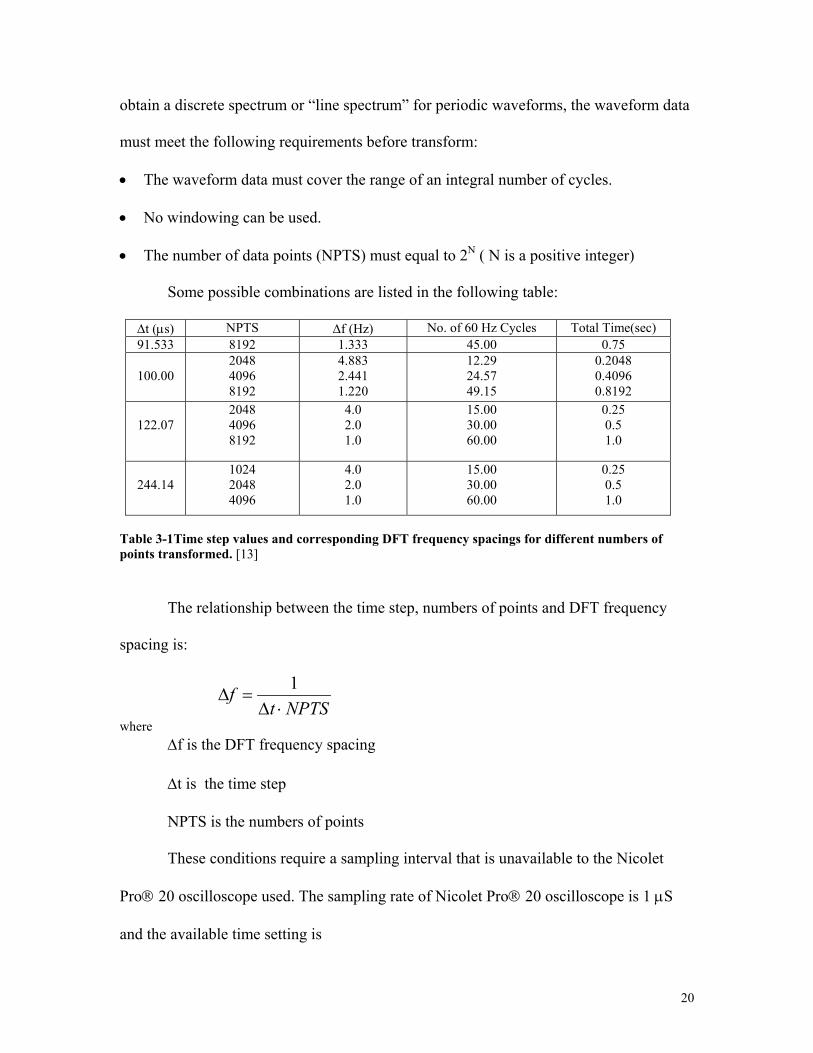
20
obtain a discrete spectrum or “line spectrum” for periodic waveforms, the waveform data
must meet the following requirements before transform:
• The waveform data must cover the range of an integral number of cycles.
• No windowing can be used.
• The number of data points (NPTS) must equal to 2N ( N is a positive integer)
Some possible combinations are listed in the following table:
∆t (µs) NPTS ∆f (Hz) No. of 60 Hz Cycles Total Time(sec) 91.533 8192 1.333 45.00 0.75
100.00
2048 4096 8192
4.883 2.441 1.220
12.29 24.57 49.15
0.2048 0.4096 0.8192
122.07
2048 4096 8192
4.0 2.0 1.0
15.00 30.00 60.00
0.25 0.5 1.0
244.14
1024 2048 4096
4.0 2.0 1.0
15.00 30.00 60.00
0.25 0.5 1.0
Table 3-1Time step values and corresponding DFT frequency spacings for different numbers of points transformed. [13]
The relationship between the time step, numbers of points and DFT frequency
spacing is:
NPTSt
f⋅∆
=∆1
where ∆f is the DFT frequency spacing
∆t is the time step
NPTS is the numbers of points
These conditions require a sampling interval that is unavailable to the Nicolet
Pro 20 oscilloscope used. The sampling rate of Nicolet Pro 20 oscilloscope is 1 µS
and the available time setting is
21
∆T = 1, 2, 5 µS;
10, 20, 50 µS;
100, 200, 500 µS
…
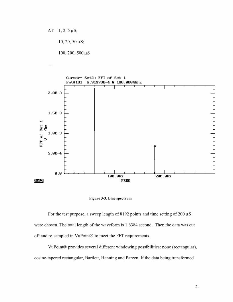
Figure 3-3. Line spectrum
For the test purpose, a sweep length of 8192 points and time setting of 200 µS
were chosen. The total length of the waveform is 1.6384 second. Then the data was cut
off and re-sampled in VuPoint to meet the FFT requirements.
VuPoint provides several different windowing possibilities: none (rectangular),
cosine-tapered rectangular, Bartlett, Hanning and Parzen. If the data being transformed
22
was an integer number of waveform cycles, a rectangular window with no tapering was
sufficient.
For the processing of harmonic test data, the last row in Table 3.1 was used. In
VuPoint, the data was first interpolated to a sampling time of 244.14 µS, then cut off to
only 1 second long. The FFT result is a perfect discrete spectrum (line spectrum). (Figure
3.3)
3.6. SPECIAL CONSIDERATION IN THE TESTS
The AM 503 current probe used requires a degauss function before
measurements. It removes any residual magnetism from the attached current probe and it
initiates an operation to remove any undesired DC offsets from probe circuitry. This
operation is recommend each time a new measurement is started or any setting on the
probe is changed.
The short-circuit tests for the 2 kVA transformer were done both manually and
automatically. The manual test was done continuously. At each frequency, the test was
repeated three times and the average value was recorded. The automatic test procedure is
discussed thoroughly in [18].
The short-circuit tests for the 10 kVA transformer was done only manually
because of the limitation of the voltage output of the Power source. At each frequency
point, only one measurement was made. But the whole test sequence was repeated three
times in different order. The first and the third test were done from high frequency to low
frequency while the second was done from low frequency to high frequency. The average
values were used for analysis.
23
________________________________________________
CHAPTER 4
TEST RESULTS AND ANALYSIS ________________________________________________
This chapter presents the test results obtained from the test setup developed in
chapter 3. Detailed analysis of the test results is provided. The test results can be found in
Appendix A through Appendix C.
4.1 LINEARITY
Because the voltage limitation of the power source, when doing the short-circuit
test, the rated current of the test transformer may not be reached at high frequencies.
Because only resistance is our concern, an alternative way is to do the short-circuit test at
lower voltage level if the linearity of the resistance holds. A check on the linearity of
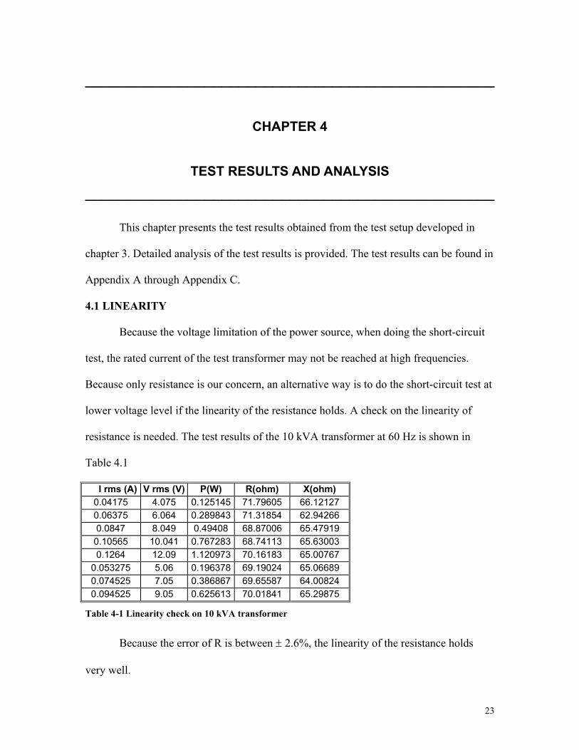
resistance is needed. The test results of the 10 kVA transformer at 60 Hz is shown in
Table 4.1
I rms (A) V rms (V) P(W) R(ohm) X(ohm) 0.04175 4.075 0.125145 71.79605 66.12127 0.06375 6.064 0.289843 71.31854 62.94266 0.0847 8.049 0.49408 68.87006 65.47919 0.10565 10.041 0.767283 68.74113 65.63003 0.1264 12.09 1.120973 70.16183 65.00767
0.053275 5.06 0.196378 69.19024 65.06689 0.074525 7.05 0.386867 69.65587 64.00824 0.094525 9.05 0.625613 70.01841 65.29875
Table 4-1 Linearity check on 10 kVA transformer
Because the error of R is between ± 2.6%, the linearity of the resistance holds
very well.
24
4.2 SUPERPOSITION
As described in Chapter 2, the UL definition of the K-factor is based on several
assumptions. One of them is that superposition of eddy current losses will apply, which
will permit the direct addition of eddy losses due to the various harmonic. This
assumption could be checked by a test described below:
First, a group of harmonics is applied to the transformer together. The voltage and
current waveforms are recorded. The load loss is measured as Pgroup. An FFT is then used
on the voltage waveform to get the amplitude and the frequency of the individual
harmonics in the group. Then individual harmonic in the group is applied to the
transformer one by one at the same amplitude and frequency, the load losses are recorded
as Pindividual. If the sum of the Pindividual is equal to Pgroup, the superposition assumption is
correct.
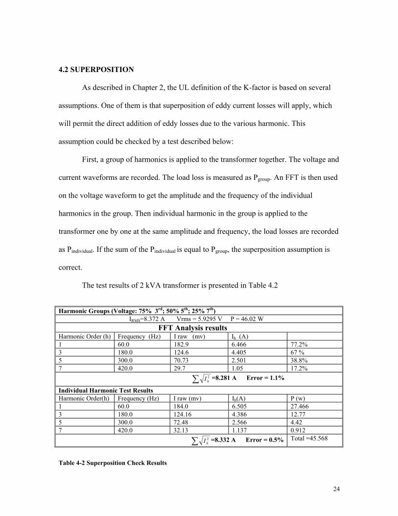
The test results of 2 kVA transformer is presented in Table 4.2
Harmonic Groups (Voltage: 75% 3rd; 50% 5th; 25% 7th) IRMS=8.372 A Vrms = 5.9295 V P = 46.02 W FFT Analysis results Harmonic Order (h) Frequency (Hz) I raw (mv) Ih (A) 1 60.0 182.9 6.466 77.2% 3 180.0 124.6 4.405 67 % 5 300.0 70.73 2.501 38.8% 7 420.0 29.7 1.05 17.2% ∑ 2
hI =8.281 A Error = 1.1%
Individual Harmonic Test Results Harmonic Order(h) Frequency (Hz) I raw (mv) Ih(A) P (w) 1 60.0 184.0 6.505 27.466 3 180.0 124.16 4.386 12.77 5 300.0 72.48 2.566 4.42 7 420.0 32.13 1.137 0.912
∑ 2hI =8.332 A Error = 0.5% Total =45.568
Table 4-2 Superposition Check Results
25
The error is (45.568 – 46.02)/46.02*100% = 0.98% which is small enough to
verify the superposition assumption is correct.
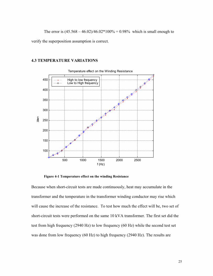
4.3 TEMPERATURE VARIATIONS
500 1000 1500 2000 2500
100
150
200
250
300
350
400
450
f (Hz)
Rac
Temperature effect on the Winding Resistance
High to low frequencyLow to High frequency
Figure 4-1 Temperature effect on the winding Resistance
Because when short-circuit tests are made continuously, heat may accumulate in the
transformer and the temperature in the transformer winding conductor may rise which
will cause the increase of the resistance. To test how much the effect will be, two set of
short-circuit tests were performed on the same 10 kVA transformer. The first set did the
test from high frequency (2940 Hz) to low frequency (60 Hz) while the second test set
was done from low frequency (60 Hz) to high frequency (2940 Hz). The results are
26
plotted in Figure 4.1. There is a small difference between the two sets of test results. The
difference is small enough to be ignored.
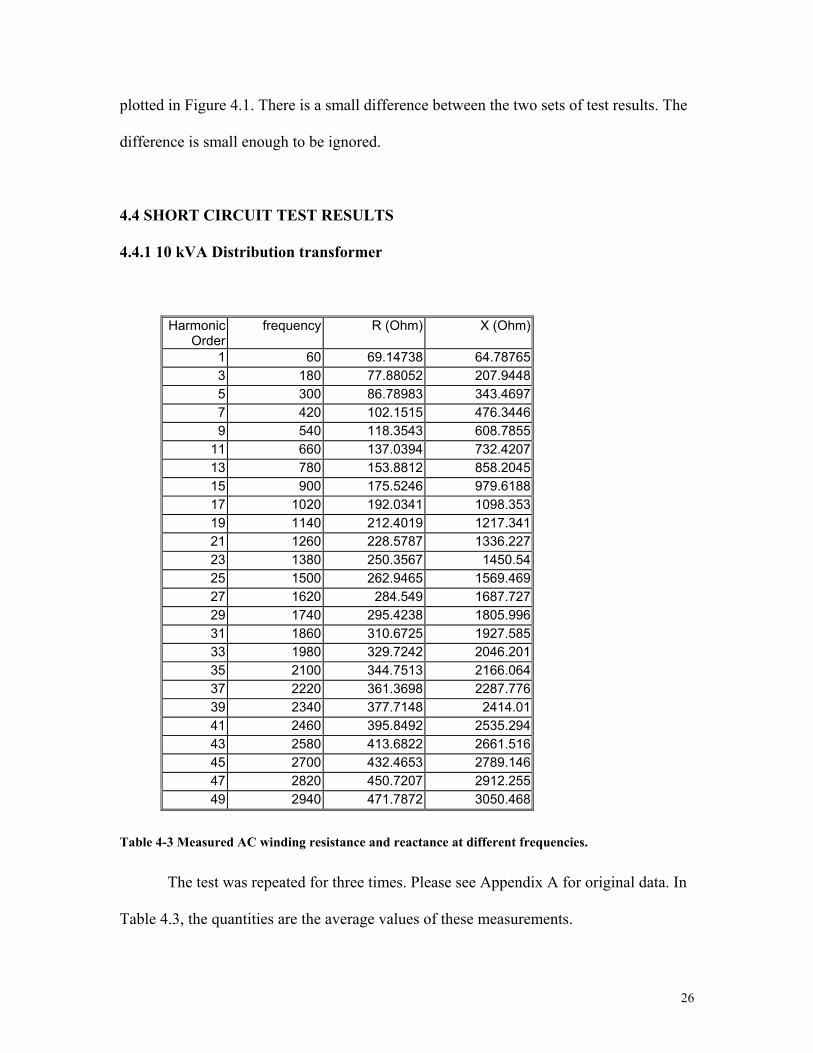
4.4 SHORT CIRCUIT TEST RESULTS 4.4.1 10 kVA Distribution transformer
Harmonic Order
frequency R (Ohm) X (Ohm)
1 60 69.14738 64.787653 180 77.88052 207.94485 300 86.78983 343.46977 420 102.1515 476.34469 540 118.3543 608.7855
11 660 137.0394 732.420713 780 153.8812 858.204515 900 175.5246 979.618817 1020 192.0341 1098.35319 1140 212.4019 1217.34121 1260 228.5787 1336.22723 1380 250.3567 1450.5425 1500 262.9465 1569.46927 1620 284.549 1687.72729 1740 295.4238 1805.99631 1860 310.6725 1927.58533 1980 329.7242 2046.20135 2100 344.7513 2166.06437 2220 361.3698 2287.77639 2340 377.7148 2414.0141 2460 395.8492 2535.29443 2580 413.6822 2661.51645 2700 432.4653 2789.14647 2820 450.7207 2912.25549 2940 471.7872 3050.468
Table 4-3 Measured AC winding resistance and reactance at different frequencies.
The test was repeated for three times. Please see Appendix A for original data. In
Table 4.3, the quantities are the average values of these measurements.
27
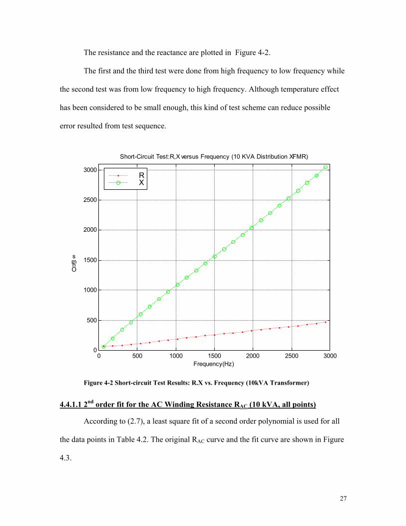
The resistance and the reactance are plotted in Figure 4-2.
The first and the third test were done from high frequency to low frequency while
the second test was from low frequency to high frequency. Although temperature effect
has been considered to be small enough, this kind of test scheme can reduce possible
error resulted from test sequence.
0 500 1000 1500 2000 2500 30000
500
1000
1500
2000
2500
3000
Frequency(Hz)
Ohms
Short-Circuit Test:R,X versus Frequency (10 KVA Distribution XFMR)
RX
Figure 4-2 Short-circuit Test Results: R.X vs. Frequency (10kVA Transformer)
4.4.1.1 2nd order fit for the AC Winding Resistance RAC (10 kVA, all points)
According to (2.7), a least square fit of a second order polynomial is used for all
the data points in Table 4.2. The original RAC curve and the fit curve are shown in Figure
4.3.
28
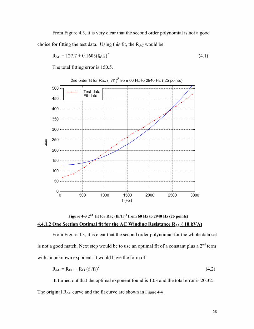
From Figure 4.3, it is very clear that the second order polynomial is not a good
choice for fitting the test data. Using this fit, the RAC would be:
RAC = 127.7 + 0.1605(fh/f1)2 (4.1)
The total fitting error is 150.5.
0 500 1000 1500 2000 2500 30000
50
100
150
200
250
300
350
400
450
500
f (Hz)
Rac
2nd order fit for Rac (fh/f1)2 from 60 Hz to 2940 Hz ( 25 points)
Test dataFit data
Figure 4-3 2nd fit for Rac (fh/f1)2 from 60 Hz to 2940 Hz (25 points)
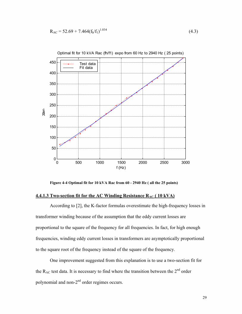
4.4.1.2 One Section Optimal fit for the AC Winding Resistance RAC ( 10 kVA)
From Figure 4.3, it is clear that the second order polynomial for the whole data set
is not a good match. Next step would be to use an optimal fit of a constant plus a 2nd term
with an unknown exponent. It would have the form of
RAC = RDC + REC(fh/f1)x (4.2)
It turned out that the optimal exponent found is 1.03 and the total error is 20.32.
The original RAC curve and the fit curve are shown in Figure 4-4
29
RAC = 52.69 + 7.464(fh/f1)1.034 (4.3)
0 500 1000 1500 2000 2500 30000
50
100
150
200
250
300
350
400
450
f (Hz)
Rac
Optimal fit for 10 kVA Rac (fh/f1) expo from 60 Hz to 2940 Hz ( 25 points)
Test dataFit data
Figure 4-4 Optimal fit for 10 kVA Rac from 60 - 2940 Hz ( all the 25 points)
4.4.1.3 Two-section fit for the AC Winding Resistance RAC ( 10 kVA)
According to [2], the K-factor formulas overestimate the high-frequency losses in
transformer winding because of the assumption that the eddy current losses are
proportional to the square of the frequency for all frequencies. In fact, for high enough
frequencies, winding eddy current losses in transformers are asymptotically proportional
to the square root of the frequency instead of the square of the frequency.
One improvement suggested from this explanation is to use a two-section fit for
the RAC test data. It is necessary to find where the transition between the 2nd order
polynomial and non-2nd order regimes occurs.
30
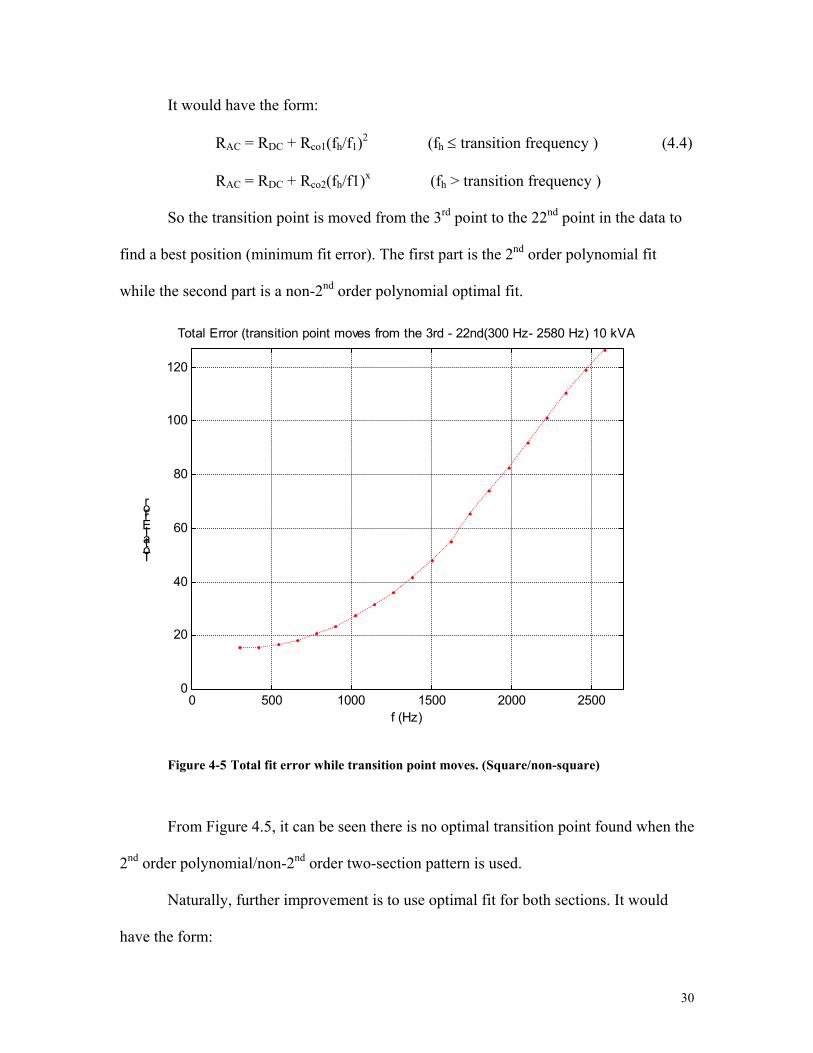
It would have the form:
RAC = RDC + Rco1(fh/f1)2 (fh ≤ transition frequency ) (4.4)
RAC = RDC + Rco2(fh/f1)x (fh > transition frequency )
So the transition point is moved from the 3rd point to the 22nd point in the data to
find a best position (minimum fit error). The first part is the 2nd order polynomial fit
while the second part is a non-2nd order polynomial optimal fit.
0 500 1000 1500 2000 25000
20
40
60
80
100
120
f (Hz)
Total Error
Total Error (transition point moves from the 3rd - 22nd(300 Hz- 2580 Hz) 10 kVA
Figure 4-5 Total fit error while transition point moves. (Square/non-square)
From Figure 4.5, it can be seen there is no optimal transition point found when the
2nd order polynomial/non-2nd order two-section pattern is used.
Naturally, further improvement is to use optimal fit for both sections. It would
have the form:
31
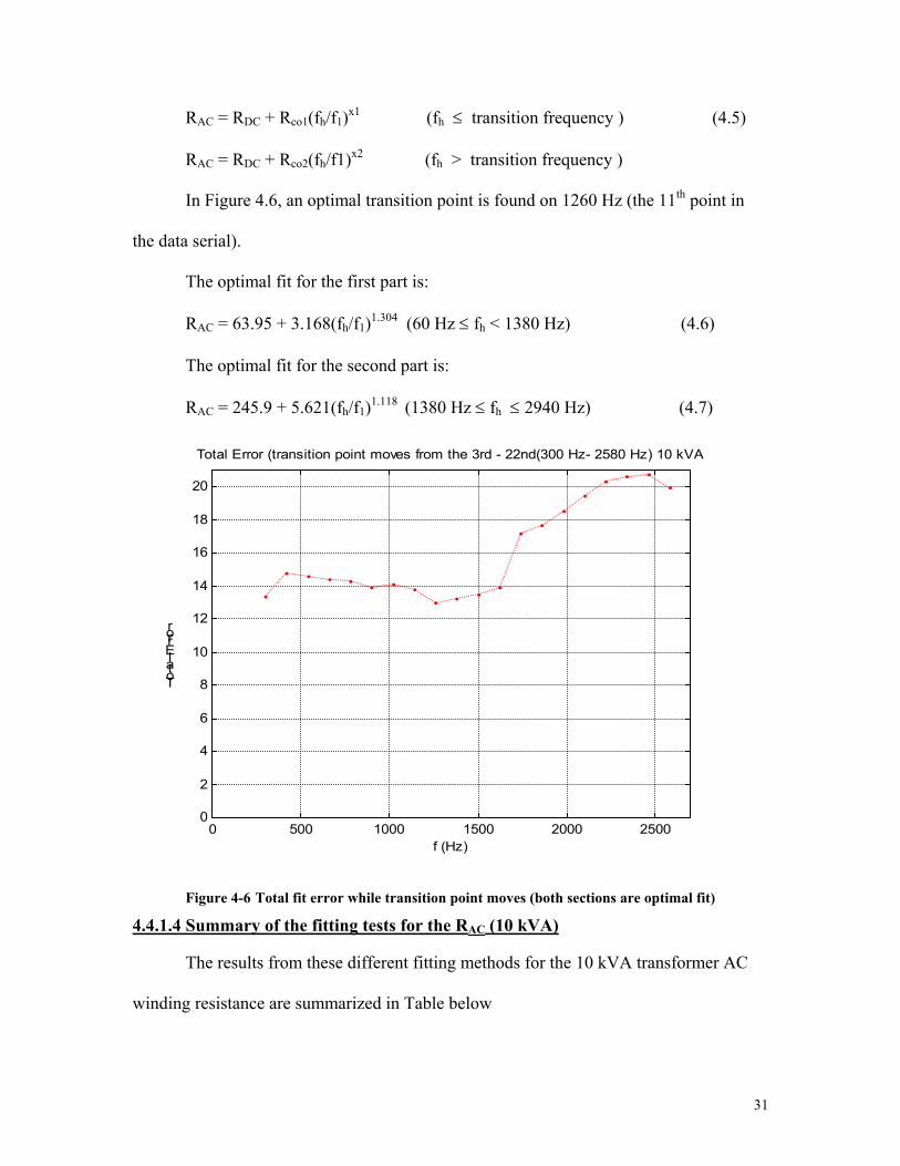
RAC = RDC + Rco1(fh/f1)x1 (fh ≤ transition frequency ) (4.5)
RAC = RDC + Rco2(fh/f1)x2 (fh > transition frequency )
In Figure 4.6, an optimal transition point is found on 1260 Hz (the 11th point in
the data serial).
The optimal fit for the first part is:
RAC = 63.95 + 3.168(fh/f1)1.304 (60 Hz ≤ fh < 1380 Hz) (4.6)
The optimal fit for the second part is:
RAC = 245.9 + 5.621(fh/f1)1.118 (1380 Hz ≤ fh ≤ 2940 Hz) (4.7)
0 500 1000 1500 2000 25000
2
4
6
8
10
12
14
16
18
20
f (Hz)
Total Error
Total Error (transition point moves from the 3rd - 22nd(300 Hz- 2580 Hz) 10 kVA
Figure 4-6 Total fit error while transition point moves (both sections are optimal fit)
4.4.1.4 Summary of the fitting tests for the RAC (10 kVA)
The results from these different fitting methods for the 10 kVA transformer AC
winding resistance are summarized in Table below
32
Exponent Fitting Method Section 1 Section 2
Error
One section (total 25 points) 2 150.5One Section (total 25points) Optimal found = 1.034 20.32Two sections(first fixed at 2) Best transition points not found N/ATwo sections (both optimal) 1.304 1.118 13.0
Table 4-4 Fitting methods comparison for 10 kVA Transformer data
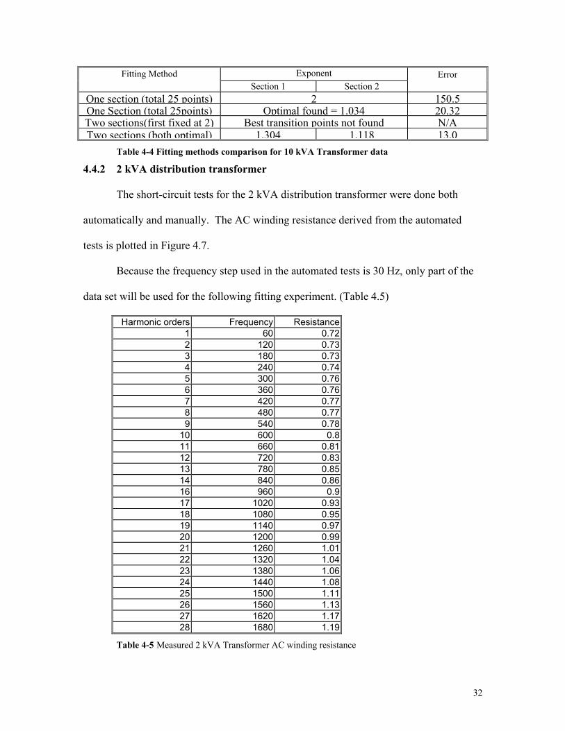
4.4.2 2 kVA distribution transformer
The short-circuit tests for the 2 kVA distribution transformer were done both
automatically and manually. The AC winding resistance derived from the automated
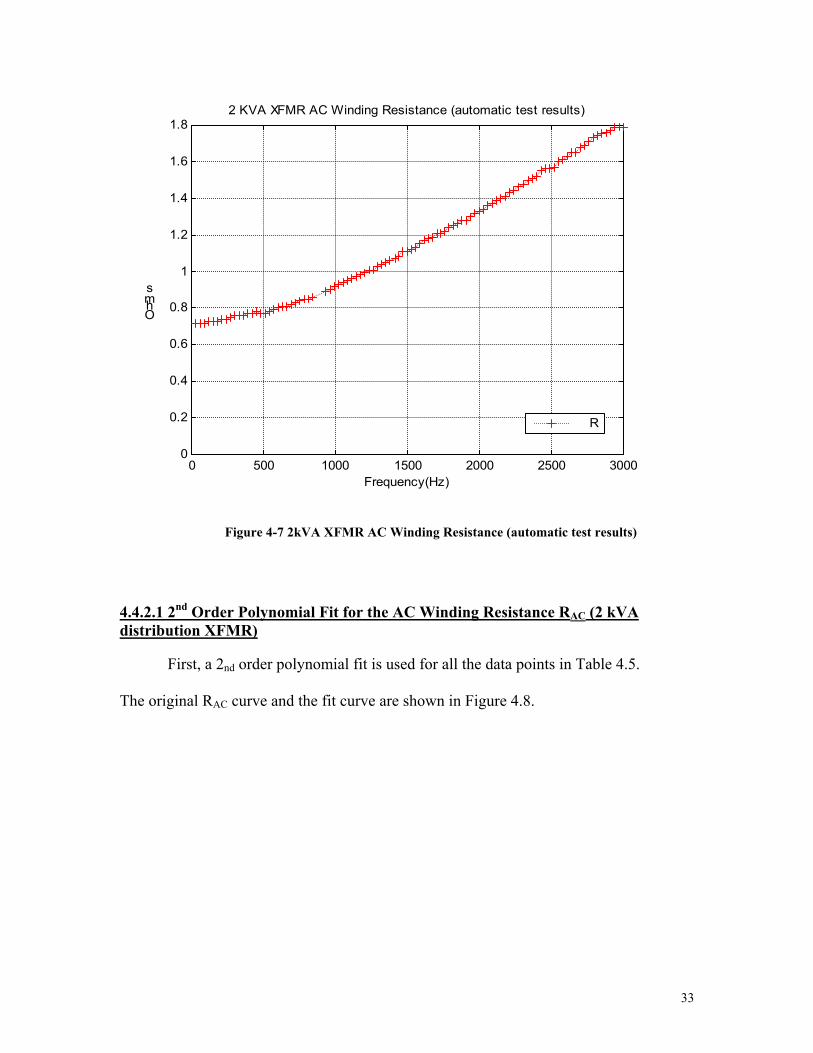
tests is plotted in Figure 4.7.
Because the frequency step used in the automated tests is 30 Hz, only part of the
data set will be used for the following fitting experiment. (Table 4.5)
Harmonic orders Frequency Resistance 1 60 0.722 120 0.733 180 0.734 240 0.745 300 0.766 360 0.767 420 0.778 480 0.779 540 0.78
10 600 0.811 660 0.8112 720 0.8313 780 0.8514 840 0.8616 960 0.917 1020 0.9318 1080 0.9519 1140 0.9720 1200 0.9921 1260 1.0122 1320 1.0423 1380 1.0624 1440 1.0825 1500 1.1126 1560 1.1327 1620 1.1728 1680 1.19
Table 4-5 Measured 2 kVA Transformer AC winding resistance
33
0 500 1000 1500 2000 2500 30000
0.2
0.4
0.6
0.8
1
1.2
1.4
1.6
1.8
Frequency(Hz)
Ohms
2 KVA XFMR AC Winding Resistance (automatic test results)
R
Figure 4-7 2kVA XFMR AC Winding Resistance (automatic test results) 4.4.2.1 2nd Order Polynomial Fit for the AC Winding Resistance RAC (2 kVA distribution XFMR)
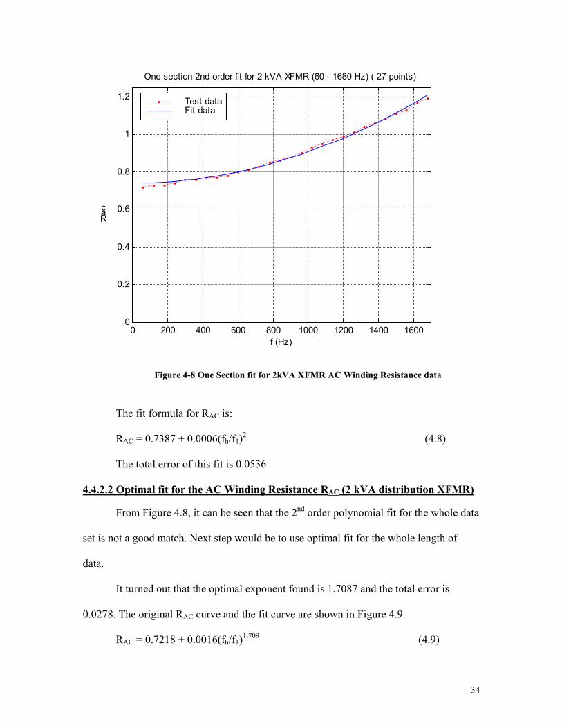
First, a 2nd order polynomial fit is used for all the data points in Table 4.5.
The original RAC curve and the fit curve are shown in Figure 4.8.
34
0 200 400 600 800 1000 1200 1400 16000
0.2
0.4
0.6
0.8
1
1.2
f (Hz)
Rac
One section 2nd order fit for 2 kVA XFMR (60 - 1680 Hz) ( 27 points)
Test dataFit data
Figure 4-8 One Section fit for 2kVA XFMR AC Winding Resistance data
The fit formula for RAC is:
RAC = 0.7387 + 0.0006(fh/f1)2 (4.8)
The total error of this fit is 0.0536
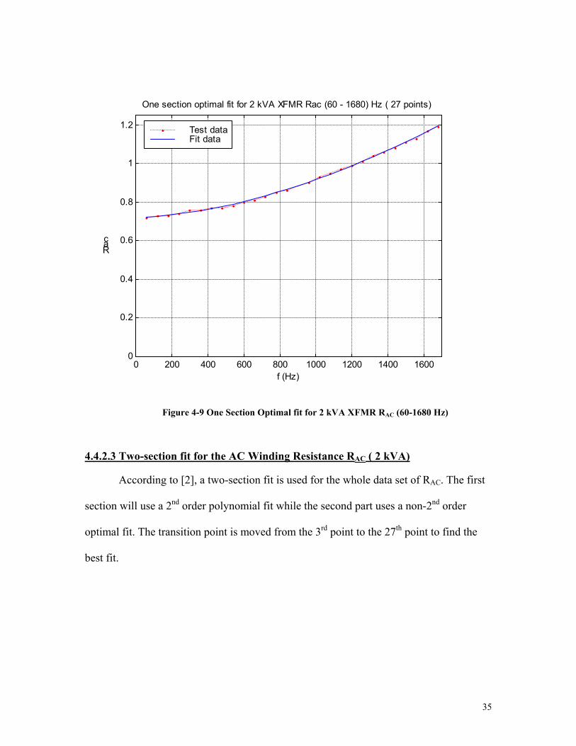
4.4.2.2 Optimal fit for the AC Winding Resistance RAC (2 kVA distribution XFMR)
From Figure 4.8, it can be seen that the 2nd order polynomial fit for the whole data
set is not a good match. Next step would be to use optimal fit for the whole length of
data.
It turned out that the optimal exponent found is 1.7087 and the total error is
0.0278. The original RAC curve and the fit curve are shown in Figure 4.9.
RAC = 0.7218 + 0.0016(fh/f1)1.709 (4.9)
35
0 200 400 600 800 1000 1200 1400 16000
0.2
0.4
0.6
0.8
1
1.2
f (Hz)
Rac
One section optimal fit for 2 kVA XFMR Rac (60 - 1680) Hz ( 27 points)
Test dataFit data
Figure 4-9 One Section Optimal fit for 2 kVA XFMR RAC (60-1680 Hz)
4.4.2.3 Two-section fit for the AC Winding Resistance RAC ( 2 kVA)
According to [2], a two-section fit is used for the whole data set of RAC. The first
section will use a 2nd order polynomial fit while the second part uses a non-2nd order
optimal fit. The transition point is moved from the 3rd point to the 27th point to find the
best fit.

36
5 10 15 20 250
0.01
0.02
0.03
0.04
0.05
0.06
Harmonic order
Total Error
Total Error when the transition point moves from 3 - 27
Figure 4-10 The total fitting error while the transition points between 2nd order fit and optimal fit moves
The total error while the transition points moves is plotted in Figure 4.10. It can
be observed that the minimum error is found when the transition point is at 1080 Hz and
the minimum error is 0.0342.
The two-section fit curve is:
RAC = 0.7296 + 0.007(fh/f1)2 (60Hz ≤ fh < 1140 Hz) (4.10)
RAC = 0.9554 + 0.0152(fh/f1)1.189 (1140Hz ≤ fh ≤ 1680 Hz)
The same process was repeated for a two-section fit which both sections use an
optimal fit.

37
The total error while the transition points moves is plotted in Figure 4.11. It can
be observed that the minimum error is found when the transition point is at 1560 Hz and
the minimum error is 0.0271.
5 10 15 20 250
0.01
0.02
0.03
0.04
0.05
0.06
Harmonic order
Total Error
Total Error when the transition point moves from 3 - 27
Figure 4-11 The total fitting error while the transition points between two optimal fit regimes moves
The two-section fit curve is:
RAC = 0.7218 + 0.0016(fh/f1)1.706 (60Hz ≤ fh < 1560 Hz) (4.11)
RAC = 1.1594 + 0.0106(fh/f1)1.531 (1560Hz ≤ fh ≤ 1680 Hz)
4.4.2.4 Summary of the fitting tests for the RAC ( 2 kVA)
The results from these different fitting methods for the 2 kVA transformer AC
winding resistance are summarized in Table 4.6.
38
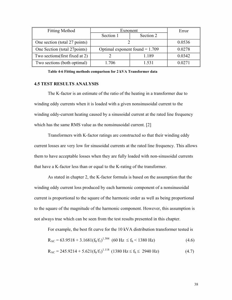
ExponentFitting Method Section 1 Section 2
Error
One section (total 27 points) 2 0.0536 One Section (total 27points) Optimal exponent found = 1.709 0.0278 Two sections(first fixed at 2) 2 1.189 0.0342 Two sections (both optimal) 1.706 1.531 0.0271
Table 4-6 Fitting methods comparison for 2 kVA Transformer data
4.5 TEST RESULTS ANALYSIS
The K-factor is an estimate of the ratio of the heating in a transformer due to
winding eddy currents when it is loaded with a given nonsinusoidal current to the
winding eddy-current heating caused by a sinusoidal current at the rated line frequency
which has the same RMS value as the nonsinusoidal current. [2]
Transformers with K-factor ratings are constructed so that their winding eddy
current losses are very low for sinusoidal currents at the rated line frequency. This allows
them to have acceptable losses when they are fully loaded with non-sinusoidal currents
that have a K-factor less than or equal to the K-rating of the transformer.
As stated in chapter 2, the K-factor formula is based on the assumption that the
winding eddy current loss produced by each harmonic component of a nonsinusoidal
current is proportional to the square of the harmonic order as well as being proportional
to the square of the magnitude of the harmonic component. However, this assumption is
not always true which can be seen from the test results presented in this chapter.
For example, the best fit curve for the 10 kVA distribution transformer tested is
RAC = 63.9518 + 3.1681(fh/f1)1.304 (60 Hz ≤ fh < 1380 Hz) (4.6)
RAC = 245.9214 + 5.621(fh/f1)1.118 (1380 Hz ≤ fh ≤ 2940 Hz) (4.7)
39
So at lower frequencies the exponent of (fh/f)ε is about ε = 1.3037 and at higher
frequencies this exponent is even smaller.
A better approach can be obtained by relaxing the limitation in the definition of
the K-factor. The power of the harmonic order should not be limited to 2. The Kε
definition is more appropriate.
∑∞
=
=1
2)( )(
hpuh hIK ε
ε (2.13)
From (2.7)-(2.10), the K-factor calculated for this transformer is apparently
conservative in the sense of derating.
Part of the reason that the exponent ε is less than 2 is that in (2.2)
Pload = I2RDC + PEC + POSL (4.2)
The other stray loss (POSL) was ignored when defining K-factor. So the actual
winding eddy-current loss is
PEC-A=(PEC + POSL) (4.12)
Because POSL are proportional to the square of the load current while not
proportional to the square of the harmonic frequency, the total PEC-A is not proportional to
the square of the harmonic frequency.
Another weak point of the K-factor formula is that it overestimates the high-
frequency losses in transformer windings. According to formulas in [16], for high enough
frequencies, winding eddy current losses in transformers are not proportional to the
square of the frequency. The geometry of the windings in a given transformer determines
when the transition between the square and the non-square regimes occurs.
As stated in Chapter 2, an important improvement the Harmonic Loss Factor
made is separating other stray loss (POSL) from winding stray loss (PEC)
40
Because the other stray losses can not be ignored, in [17], an assumption is made
to estimate the portion of the other stray losses.
a) 67% of the total stray loss is assumed to be winding eddy losses for dry-type
transformers and 33% of the total stray loss is assumed to be the other stray
loss.
b) 33% of the total stay loss is assumed to be winding eddy losses for oil-filled
transformers and 67% of the total stray loss is assumed to be the other stray
loss.
This assumption can be checked using an optimal search. Using the assumption
that the winding eddy-current loss vary with the square of the frequency and the other
stray loss vary with the frequency raised to the 0.8 power, the fit formula is:
RAC = RDC + β1h2 + β2h0.8
It is found these assumptions are not accurate for the tested transformer but it can
help explain the difference of the exponent of (fh/f)ε between 2 kVA dry-type transformer
and 10 kVA oil-filled transformer.
For the 2 kVA dry-type transformer, at low frequencies
RAC = 0.7218 + 0.0016(fh/f1)1.706 (60Hz ≤ fh < 1560 Hz) (4.11)
For the 10 kVA oil-filled transformer, at low frequencies
RAC = 63.95 + 3.168(fh/f1)1.304 (60 Hz ≤ fh < 1380 Hz) (4.6)
In the dry-type transformer, the winding eddy losses, which is assumed
proportional to the square of the frequency, takes a larger part in the total stray loss than
in the oil-filled transformer, the exponent of (fh/f)ε found is larger.
41
________________________________________________
CHAPTER 5
CONCLUSIONS AND RECOMMENDATION
_______________________________________________________
This chapter presents the conclusions drawn from this work. Topics including
closing comments regarding the lab tests, the K-factor concept and the Harmonic Loss
Factor (FHL). Recommendations for future work are also provided.
5.1 CONCLUSIONS • The K-factor does not apply to the two tested transformer and overestimates the
losses in transformer windings because the winding eddy current losses in
transformers tested are not proportional to the square of the frequency, instead, they
are proportional to a power of the frequency which is less than 2.
• For the two transformers tested, the eddy-current loss is a function of frequency with
power less than 2 so an alternative definition of the K factor, Kε, in which the
exponent ε is less than 2 is better.
• The Harmonic Loss Factor is a better approach for estimating transformer load loss.
Compared with the K-factor, the Harmonic Loss Factor is a function of the harmonic
current distribution and is independent of the relative magnitude while the K-factor is
dependent on both the magnitude and distribution of the harmonics. Harmonic Loss
Factor also has a separate definition for the other stray losses assuming that they are

42
proportional to the square of the load current magnitude and the harmonic frequency
to the 0.8 power.
5.2 RECOMMENDATIONS FOR FUTURE WORK
More laboratory tests on different transformers are needed. A detailed study of
transformer structure such as the geometry of the windings is necessary for further study.
A laboratory test method for separating winding eddy current losses from stray
losses in components other than windings are important in the future work.
43
Reference: [1] "An American National Standard: IEEE Recommended Practice for Establishing
Transformer Capability When Supplying Nonsinusoidal Load Currents."
ANSI/IEEE C57.110-1986
[2] Bryce Hesterman, "Time-Domain K-Factor Computation Methods", 29th
International Power Conversion Conference, September 1994, pp.406-417
[3] Tom Shaughnessy, "Use Derating and K-Factor Calculation Carefully", Power
Quality Assurance, March/April 1994, pp.36-41.
[4] E.F.Fuchs, D.Yildirim, and W.M.Grady, "Measurement of Eddy-Current Loss
Coefficient PEC-R, Derating of Single-Phase Transformers, and Comparison with K-
Factor Approach", IEEE Trans on Power Delivery, Paper # 99WM104, accepted
for publication.
[5] D.Yildirim and E.F.Fuchs, “Measured Transformer Derating and Comparison with
Harmonic Loss Factor (FHL) Approach”, PE-084-PWRD-0-03-1999.
[6] Jerome M. Frank, “Origin, Development, and Design of K-Factor Transformers”,
IEEE Industry Applications Magazine, September/October, 1997, pp67-69
[7] A.W.Galli and M.D.Cox, “Temperature Rise of Small Oil-filled Distribution
Transformers Supplying Nonsinusoidal Load Currents”, IEEE Transaction on
Power Delivery, January 1996, Vol.11, No.1, pp. 283-291
[8] M.T.Bishop, J.F.Baranowshki, D.Heath and S.J.Benna, “Evaluating Harmonic-
Induced Transformer Heating,” IEEE Transaction on Power Delivery”, January
1996, Vol.11, No.1, pp. 305-311.
44
[9] Keith H. Sueker, “Comments on ‘Harmonics: The Effects on Power Quality and
Transformers’”, IEEE Transaction on Industry Applications, March/April 1995,
Vol.31, No.2, pp. 405-406.
[10] Gregory W. Massey, “Estimation Methods for Power System Harmonic Effects on
Power Distribution Transformers”, IEEE Transaction on Industry Applications,
March/April 1994, Vol. 30, No.2, pp. 485-489.
[11] “AMX Series AC Power Source Operation Manual”, Pacific Power Source, Oct,
1996.
[12] “UPC-32/UPC-12 Operation Manual”, Pacific Power Source, Jan, 1995.
[13] Bruce Andrew Mork, “Ferroresonance and Chaos: Observation and Simulation of
Ferroresonance in a Five-Legged core distribution transformer”, Ph.D. Thesis, May
1992, Fargo, North Dakota, pp240.
[14] Standard UL1561, “Dry-Type General Purpose and Power Transformers”, April 22,
1994.
[15] Standard UL1562, “Transformers, Distribution, Dry-Type-Over 600 Volts”, 1994
[16] P.L.Dowell, “Effects of Eddy Currents in Transformer Windings” Proceedings of
the IEE, Vol 112, No.8 Aug. 1966, pp. 1387-1394.
[17] "ANSI/IEEE Recommended Practice for Establishing Transformer Capability When
Supplying Nonsinusoidal Load Currents." ANSI/IEEE C57.110/D7-February 1998,
Institute of Electrical and Electronics Engineers, Inc., New York, NY, 1998.
[18] Manjunatha Rao, “Development of a Laboratory Test Setup Using LabView for a
Power Quality Study”, MS Report, Michigan Tech University, 1999.

45
[19] Michael J. Gaffney, “Amorphous Core Transformer Model for Transient
Simulation”, MS Thesis, Michigan Tech University, 1996.
[20] Michael A. Bjorge, “Investigation of Short-Circuit Models for A Four-Winding
Transformer”, MS Thesis, Michigan Tech University, 1996.
[21] Richard L. Bean, “Transformers for the Electric Power Industry”, McGraw-Hill
Book Company, Inc., 1959.
46
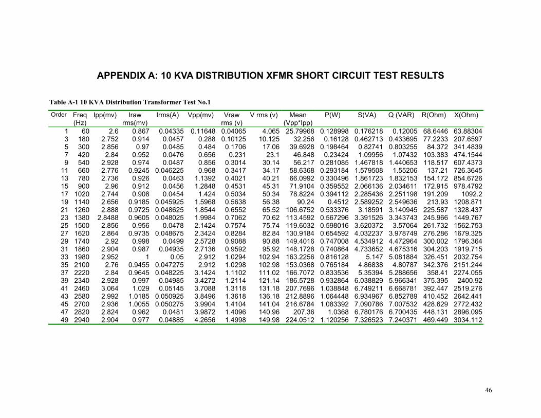
APPENDIX A: 10 KVA DISTRIBUTION XFMR SHORT CIRCUIT TEST RESULTS
Table A-1 10 KVA Distribution Transformer Test No.1
Order Freq (Hz)
Ipp(mv) Iraw rms(mv)
Irms(A) Vpp(mv) Vraw rms (v)
V rms (v) Mean (Vpp*Ipp)
P(W) S(VA) Q (VAR) R(Ohm) X(Ohm)
1 60 2.6 0.867 0.04335 0.11648 0.04065 4.065 25.79968 0.128998 0.176218 0.12005 68.6446 63.883043 180 2.752 0.914 0.0457 0.288 0.10125 10.125 32.256 0.16128 0.462713 0.433695 77.2233 207.65975 300 2.856 0.97 0.0485 0.484 0.1706 17.06 39.6928 0.198464 0.82741 0.803255 84.372 341.48397 420 2.84 0.952 0.0476 0.656 0.231 23.1 46.848 0.23424 1.09956 1.07432 103.383 474.15449 540 2.928 0.974 0.0487 0.856 0.3014 30.14 56.217 0.281085 1.467818 1.440653 118.517 607.4373
11 660 2.776 0.9245 0.046225 0.968 0.3417 34.17 58.6368 0.293184 1.579508 1.55206 137.21 726.364513 780 2.736 0.926 0.0463 1.1392 0.4021 40.21 66.0992 0.330496 1.861723 1.832153 154.172 854.672615 900 2.96 0.912 0.0456 1.2848 0.4531 45.31 71.9104 0.359552 2.066136 2.034611 172.915 978.479217 1020 2.744 0.908 0.0454 1.424 0.5034 50.34 78.8224 0.394112 2.285436 2.251198 191.209 1092.219 1140 2.656 0.9185 0.045925 1.5968 0.5638 56.38 90.24 0.4512 2.589252 2.549636 213.93 1208.87121 1260 2.888 0.9725 0.048625 1.8544 0.6552 65.52 106.6752 0.533376 3.18591 3.140945 225.587 1328.43723 1380 2.8488 0.9605 0.048025 1.9984 0.7062 70.62 113.4592 0.567296 3.391526 3.343743 245.966 1449.76725 1500 2.856 0.956 0.0478 2.1424 0.7574 75.74 119.6032 0.598016 3.620372 3.57064 261.732 1562.75327 1620 2.864 0.9735 0.048675 2.3424 0.8284 82.84 130.9184 0.654592 4.032237 3.978749 276.286 1679.32529 1740 2.92 0.998 0.0499 2.5728 0.9088 90.88 149.4016 0.747008 4.534912 4.472964 300.002 1796.36431 1860 2.904 0.987 0.04935 2.7136 0.9592 95.92 148.1728 0.740864 4.733652 4.675316 304.203 1919.71533 1980 2.952 1 0.05 2.912 1.0294 102.94 163.2256 0.816128 5.147 5.081884 326.451 2032.75435 2100 2.76 0.9455 0.047275 2.912 1.0298 102.98 153.0368 0.765184 4.86838 4.80787 342.376 2151.24437 2220 2.84 0.9645 0.048225 3.1424 1.1102 111.02 166.7072 0.833536 5.35394 5.288656 358.41 2274.05539 2340 2.928 0.997 0.04985 3.4272 1.2114 121.14 186.5728 0.932864 6.038829 5.966341 375.395 2400.9241 2460 3.064 1.029 0.05145 3.7088 1.3118 131.18 207.7696 1.038848 6.749211 6.668781 392.447 2519.27643 2580 2.992 1.0185 0.050925 3.8496 1.3618 136.18 212.8896 1.064448 6.934967 6.852789 410.452 2642.44145 2700 2.936 1.0055 0.050275 3.9904 1.4104 141.04 216.6784 1.083392 7.090786 7.007532 428.629 2772.43247 2820 2.824 0.962 0.0481 3.9872 1.4096 140.96 207.36 1.0368 6.780176 6.700435 448.131 2896.09549 2940 2.904 0.977 0.04885 4.2656 1.4998 149.98 224.0512 1.120256 7.326523 7.240371 469.449 3034.112
47
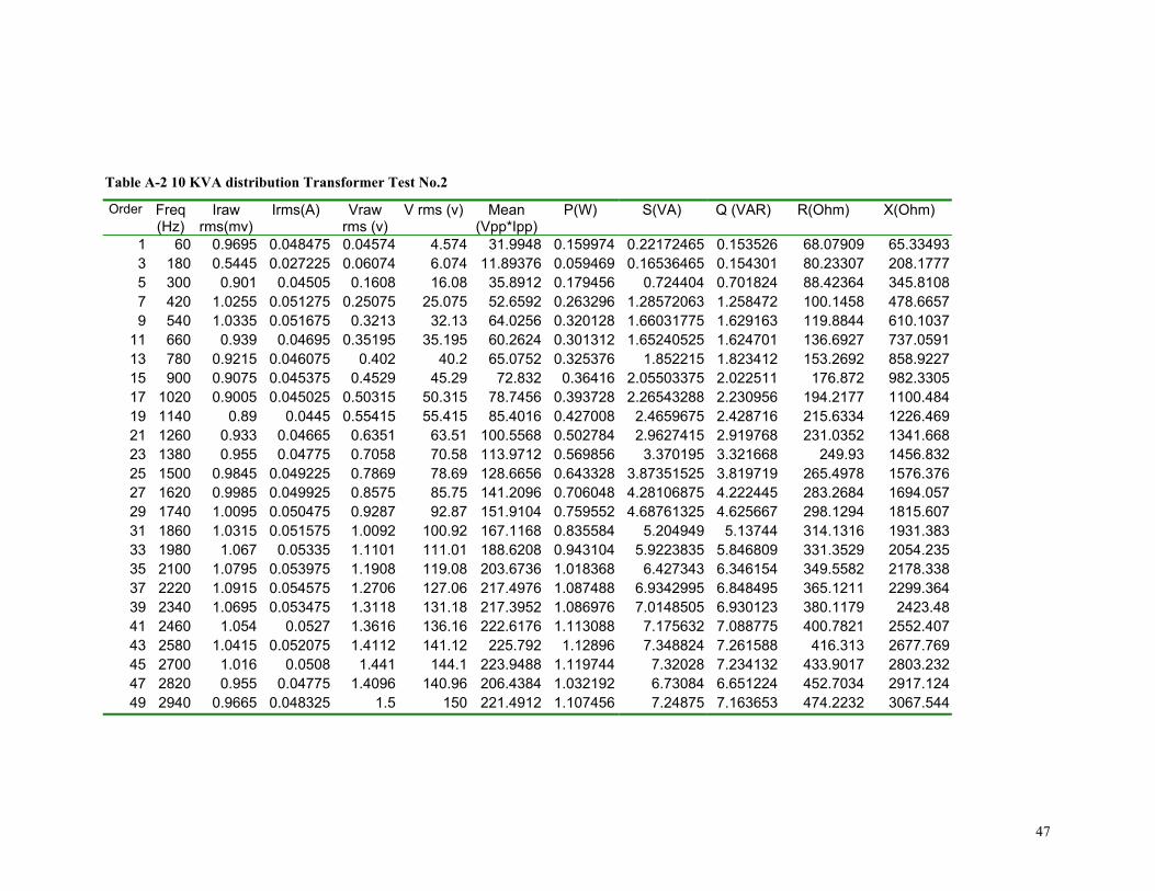
Table A-2 10 KVA distribution Transformer Test No.2
Order Freq (Hz)
Iraw rms(mv)
Irms(A) Vraw rms (v)
V rms (v) Mean (Vpp*Ipp)
P(W) S(VA) Q (VAR) R(Ohm) X(Ohm)
1 60 0.9695 0.048475 0.04574 4.574 31.9948 0.159974 0.22172465 0.153526 68.07909 65.334933 180 0.5445 0.027225 0.06074 6.074 11.89376 0.059469 0.16536465 0.154301 80.23307 208.17775 300 0.901 0.04505 0.1608 16.08 35.8912 0.179456 0.724404 0.701824 88.42364 345.81087 420 1.0255 0.051275 0.25075 25.075 52.6592 0.263296 1.28572063 1.258472 100.1458 478.66579 540 1.0335 0.051675 0.3213 32.13 64.0256 0.320128 1.66031775 1.629163 119.8844 610.1037
11 660 0.939 0.04695 0.35195 35.195 60.2624 0.301312 1.65240525 1.624701 136.6927 737.059113 780 0.9215 0.046075 0.402 40.2 65.0752 0.325376 1.852215 1.823412 153.2692 858.922715 900 0.9075 0.045375 0.4529 45.29 72.832 0.36416 2.05503375 2.022511 176.872 982.330517 1020 0.9005 0.045025 0.50315 50.315 78.7456 0.393728 2.26543288 2.230956 194.2177 1100.48419 1140 0.89 0.0445 0.55415 55.415 85.4016 0.427008 2.4659675 2.428716 215.6334 1226.46921 1260 0.933 0.04665 0.6351 63.51 100.5568 0.502784 2.9627415 2.919768 231.0352 1341.66823 1380 0.955 0.04775 0.7058 70.58 113.9712 0.569856 3.370195 3.321668 249.93 1456.83225 1500 0.9845 0.049225 0.7869 78.69 128.6656 0.643328 3.87351525 3.819719 265.4978 1576.37627 1620 0.9985 0.049925 0.8575 85.75 141.2096 0.706048 4.28106875 4.222445 283.2684 1694.05729 1740 1.0095 0.050475 0.9287 92.87 151.9104 0.759552 4.68761325 4.625667 298.1294 1815.60731 1860 1.0315 0.051575 1.0092 100.92 167.1168 0.835584 5.204949 5.13744 314.1316 1931.38333 1980 1.067 0.05335 1.1101 111.01 188.6208 0.943104 5.9223835 5.846809 331.3529 2054.23535 2100 1.0795 0.053975 1.1908 119.08 203.6736 1.018368 6.427343 6.346154 349.5582 2178.33837 2220 1.0915 0.054575 1.2706 127.06 217.4976 1.087488 6.9342995 6.848495 365.1211 2299.36439 2340 1.0695 0.053475 1.3118 131.18 217.3952 1.086976 7.0148505 6.930123 380.1179 2423.4841 2460 1.054 0.0527 1.3616 136.16 222.6176 1.113088 7.175632 7.088775 400.7821 2552.40743 2580 1.0415 0.052075 1.4112 141.12 225.792 1.12896 7.348824 7.261588 416.313 2677.76945 2700 1.016 0.0508 1.441 144.1 223.9488 1.119744 7.32028 7.234132 433.9017 2803.23247 2820 0.955 0.04775 1.4096 140.96 206.4384 1.032192 6.73084 6.651224 452.7034 2917.12449 2940 0.9665 0.048325 1.5 150 221.4912 1.107456 7.24875 7.163653 474.2232 3067.544
48
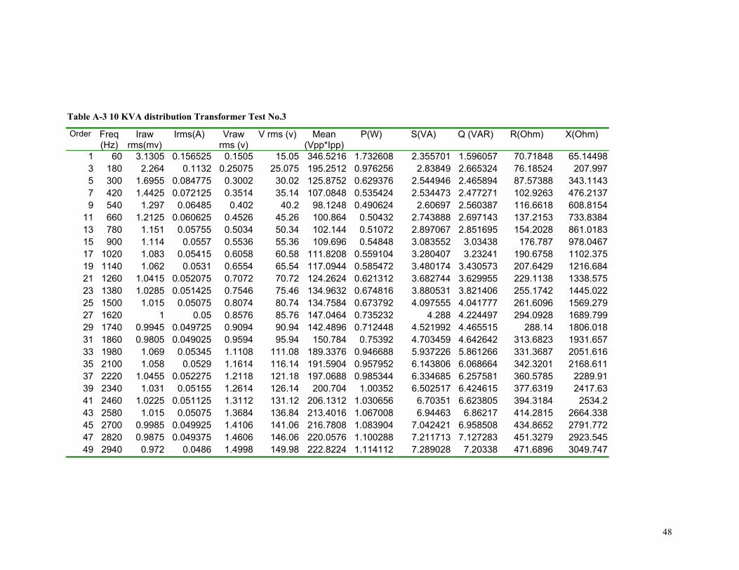
Table A-3 10 KVA distribution Transformer Test No.3
Order Freq (Hz)
Iraw rms(mv)
Irms(A) Vraw rms (v)
V rms (v) Mean (Vpp*Ipp)
P(W) S(VA) Q (VAR) R(Ohm) X(Ohm)
1 60 3.1305 0.156525 0.1505 15.05 346.5216 1.732608 2.355701 1.596057 70.71848 65.144983 180 2.264 0.1132 0.25075 25.075 195.2512 0.976256 2.83849 2.665324 76.18524 207.9975 300 1.6955 0.084775 0.3002 30.02 125.8752 0.629376 2.544946 2.465894 87.57388 343.11437 420 1.4425 0.072125 0.3514 35.14 107.0848 0.535424 2.534473 2.477271 102.9263 476.21379 540 1.297 0.06485 0.402 40.2 98.1248 0.490624 2.60697 2.560387 116.6618 608.8154
11 660 1.2125 0.060625 0.4526 45.26 100.864 0.50432 2.743888 2.697143 137.2153 733.838413 780 1.151 0.05755 0.5034 50.34 102.144 0.51072 2.897067 2.851695 154.2028 861.018315 900 1.114 0.0557 0.5536 55.36 109.696 0.54848 3.083552 3.03438 176.787 978.046717 1020 1.083 0.05415 0.6058 60.58 111.8208 0.559104 3.280407 3.23241 190.6758 1102.37519 1140 1.062 0.0531 0.6554 65.54 117.0944 0.585472 3.480174 3.430573 207.6429 1216.68421 1260 1.0415 0.052075 0.7072 70.72 124.2624 0.621312 3.682744 3.629955 229.1138 1338.57523 1380 1.0285 0.051425 0.7546 75.46 134.9632 0.674816 3.880531 3.821406 255.1742 1445.02225 1500 1.015 0.05075 0.8074 80.74 134.7584 0.673792 4.097555 4.041777 261.6096 1569.27927 1620 1 0.05 0.8576 85.76 147.0464 0.735232 4.288 4.224497 294.0928 1689.79929 1740 0.9945 0.049725 0.9094 90.94 142.4896 0.712448 4.521992 4.465515 288.14 1806.01831 1860 0.9805 0.049025 0.9594 95.94 150.784 0.75392 4.703459 4.642642 313.6823 1931.65733 1980 1.069 0.05345 1.1108 111.08 189.3376 0.946688 5.937226 5.861266 331.3687 2051.61635 2100 1.058 0.0529 1.1614 116.14 191.5904 0.957952 6.143806 6.068664 342.3201 2168.61137 2220 1.0455 0.052275 1.2118 121.18 197.0688 0.985344 6.334685 6.257581 360.5785 2289.9139 2340 1.031 0.05155 1.2614 126.14 200.704 1.00352 6.502517 6.424615 377.6319 2417.6341 2460 1.0225 0.051125 1.3112 131.12 206.1312 1.030656 6.70351 6.623805 394.3184 2534.243 2580 1.015 0.05075 1.3684 136.84 213.4016 1.067008 6.94463 6.86217 414.2815 2664.33845 2700 0.9985 0.049925 1.4106 141.06 216.7808 1.083904 7.042421 6.958508 434.8652 2791.77247 2820 0.9875 0.049375 1.4606 146.06 220.0576 1.100288 7.211713 7.127283 451.3279 2923.54549 2940 0.972 0.0486 1.4998 149.98 222.8224 1.114112 7.289028 7.20338 471.6896 3049.747

49
Table A-4 10 KVA distribution Transformer Rdc Test Results
RHV (Ω) RLV (Ω) Turns Ratio RDC (Ω)
35 0.3 30:1 44
50
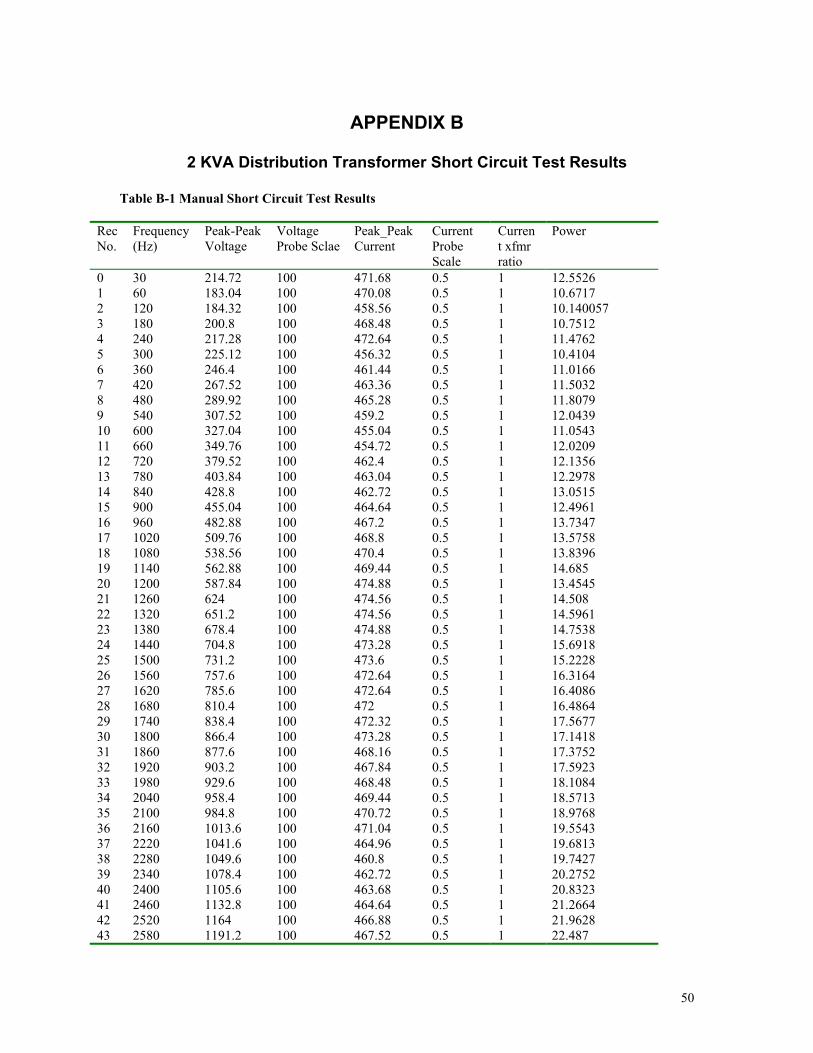
APPENDIX B
2 KVA Distribution Transformer Short Circuit Test Results Table B-1 Manual Short Circuit Test Results
Rec No.
Frequency (Hz)
Peak-Peak Voltage
Voltage Probe Sclae
Peak_Peak Current
Current Probe Scale
Current xfmr ratio
Power
0 30 214.72 100 471.68 0.5 1 12.5526 1 60 183.04 100 470.08 0.5 1 10.6717 2 120 184.32 100 458.56 0.5 1 10.140057 3 180 200.8 100 468.48 0.5 1 10.7512 4 240 217.28 100 472.64 0.5 1 11.4762 5 300 225.12 100 456.32 0.5 1 10.4104 6 360 246.4 100 461.44 0.5 1 11.0166 7 420 267.52 100 463.36 0.5 1 11.5032 8 480 289.92 100 465.28 0.5 1 11.8079 9 540 307.52 100 459.2 0.5 1 12.0439 10 600 327.04 100 455.04 0.5 1 11.0543 11 660 349.76 100 454.72 0.5 1 12.0209 12 720 379.52 100 462.4 0.5 1 12.1356 13 780 403.84 100 463.04 0.5 1 12.2978 14 840 428.8 100 462.72 0.5 1 13.0515 15 900 455.04 100 464.64 0.5 1 12.4961 16 960 482.88 100 467.2 0.5 1 13.7347 17 1020 509.76 100 468.8 0.5 1 13.5758 18 1080 538.56 100 470.4 0.5 1 13.8396 19 1140 562.88 100 469.44 0.5 1 14.685 20 1200 587.84 100 474.88 0.5 1 13.4545 21 1260 624 100 474.56 0.5 1 14.508 22 1320 651.2 100 474.56 0.5 1 14.5961 23 1380 678.4 100 474.88 0.5 1 14.7538 24 1440 704.8 100 473.28 0.5 1 15.6918 25 1500 731.2 100 473.6 0.5 1 15.2228 26 1560 757.6 100 472.64 0.5 1 16.3164 27 1620 785.6 100 472.64 0.5 1 16.4086 28 1680 810.4 100 472 0.5 1 16.4864 29 1740 838.4 100 472.32 0.5 1 17.5677 30 1800 866.4 100 473.28 0.5 1 17.1418 31 1860 877.6 100 468.16 0.5 1 17.3752 32 1920 903.2 100 467.84 0.5 1 17.5923 33 1980 929.6 100 468.48 0.5 1 18.1084 34 2040 958.4 100 469.44 0.5 1 18.5713 35 2100 984.8 100 470.72 0.5 1 18.9768 36 2160 1013.6 100 471.04 0.5 1 19.5543 37 2220 1041.6 100 464.96 0.5 1 19.6813 38 2280 1049.6 100 460.8 0.5 1 19.7427 39 2340 1078.4 100 462.72 0.5 1 20.2752 40 2400 1105.6 100 463.68 0.5 1 20.8323 41 2460 1132.8 100 464.64 0.5 1 21.2664 42 2520 1164 100 466.88 0.5 1 21.9628 43 2580 1191.2 100 467.52 0.5 1 22.487
51
44 2640 1217.6 100 468.16 0.5 1 22.8884 45 2700 1244 100 468.8 0.5 1 23.4004 46 2760 1257.6 100 464 0.5 1 23.38 47 2820 1289.6 100 466.88 0.5 1 24.0353 48 2880 1321.6 100 469.12 0.5 1 24.7685 49 2940 1348 100 469.12 0.5 1 25.3379 50 3000 1377.6 100 470.72 0.5 1 25.8908
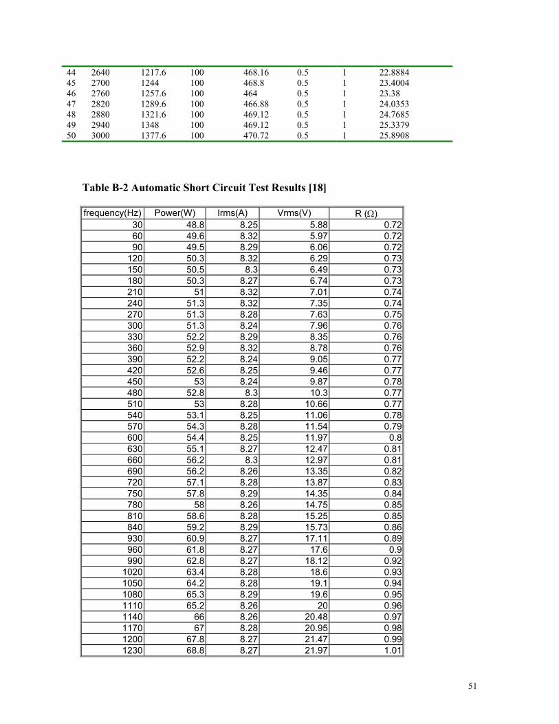
Table B-2 Automatic Short Circuit Test Results [18]
frequency(Hz) Power(W) Irms(A) Vrms(V) R (Ω) 30 48.8 8.25 5.88 0.72 60 49.6 8.32 5.97 0.72 90 49.5 8.29 6.06 0.72
120 50.3 8.32 6.29 0.73 150 50.5 8.3 6.49 0.73 180 50.3 8.27 6.74 0.73 210 51 8.32 7.01 0.74 240 51.3 8.32 7.35 0.74 270 51.3 8.28 7.63 0.75 300 51.3 8.24 7.96 0.76 330 52.2 8.29 8.35 0.76 360 52.9 8.32 8.78 0.76 390 52.2 8.24 9.05 0.77 420 52.6 8.25 9.46 0.77 450 53 8.24 9.87 0.78 480 52.8 8.3 10.3 0.77 510 53 8.28 10.66 0.77 540 53.1 8.25 11.06 0.78 570 54.3 8.28 11.54 0.79 600 54.4 8.25 11.97 0.8 630 55.1 8.27 12.47 0.81 660 56.2 8.3 12.97 0.81 690 56.2 8.26 13.35 0.82 720 57.1 8.28 13.87 0.83 750 57.8 8.29 14.35 0.84 780 58 8.26 14.75 0.85 810 58.6 8.28 15.25 0.85 840 59.2 8.29 15.73 0.86 930 60.9 8.27 17.11 0.89 960 61.8 8.27 17.6 0.9 990 62.8 8.27 18.12 0.92
1020 63.4 8.28 18.6 0.93 1050 64.2 8.28 19.1 0.94 1080 65.3 8.29 19.6 0.95 1110 65.2 8.26 20 0.96 1140 66 8.26 20.48 0.97 1170 67 8.28 20.95 0.98 1200 67.8 8.27 21.47 0.99 1230 68.8 8.27 21.97 1.01

52
1260 69.4 8.28 22.45 1.01 1290 70.5 8.28 22.94 1.03 1320 71.3 8.28 23.44 1.04 1350 72 8.29 23.92 1.05 1380 73.1 8.3 24.44 1.06 1410 73.9 8.3 24.94 1.07 1440 74.7 8.3 25.43 1.08 1470 75.2 8.25 25.82 1.11 1500 76.1 8.28 26.32 1.11 1530 76.8 8.28 26.81 1.12 1560 78.5 8.32 27.38 1.13 1590 79.6 8.32 27.88 1.15 1620 80.6 8.3 28.37 1.17 1650 80.8 8.28 28.76 1.18 1680 81.6 8.28 29.26 1.19 1710 83 8.29 29.73 1.21 1730 83.5 8.3 30.14 1.21 1760 84.4 8.3 30.61 1.22 1790 85.1 8.28 31.02 1.24 1820 86.7 8.32 31.61 1.25 1850 86.9 8.29 32 1.26 1880 88.2 8.29 32.47 1.28 1910 88.6 8.3 32.99 1.28 1940 89.5 8.3 33.44 1.3 1970 90.9 8.32 33.94 1.32 2000 91.2 8.28 34.35 1.33 2030 92.7 8.3 34.94 1.34 2060 94 8.3 35.41 1.36 2090 94.3 8.28 35.8 1.37 2120 95.5 8.29 36.29 1.39 2150 96.5 8.3 36.79 1.4 2180 97.3 8.3 37.27 1.41 2210 98.4 8.3 37.72 1.43 2240 99.6 8.3 38.22 1.44 2270 100.4 8.3 38.74 1.46 2310 101.6 8.29 39.26 1.48 2340 102.9 8.29 39.78 1.5 2370 104.3 8.32 40.39 1.51 2400 105.3 8.32 40.87 1.52 2430 106.3 8.29 41.23 1.55 2460 107.5 8.29 41.72 1.56 2490 108.2 8.32 42.11 1.56 2520 108.5 8.3 42.58 1.57 2550 109.9 8.29 43.06 1.6 2580 111.1 8.3 43.54 1.61 2610 112.5 8.3 44.06 1.63 2640 113.2 8.29 44.53 1.65 2670 113.7 8.29 44.44 1.65 2700 115 8.28 45.03 1.68 2730 116.3 8.3 45.53 1.69 2760 117.3 8.29 46.02 1.71 2790 118.5 8.28 46.39 1.73
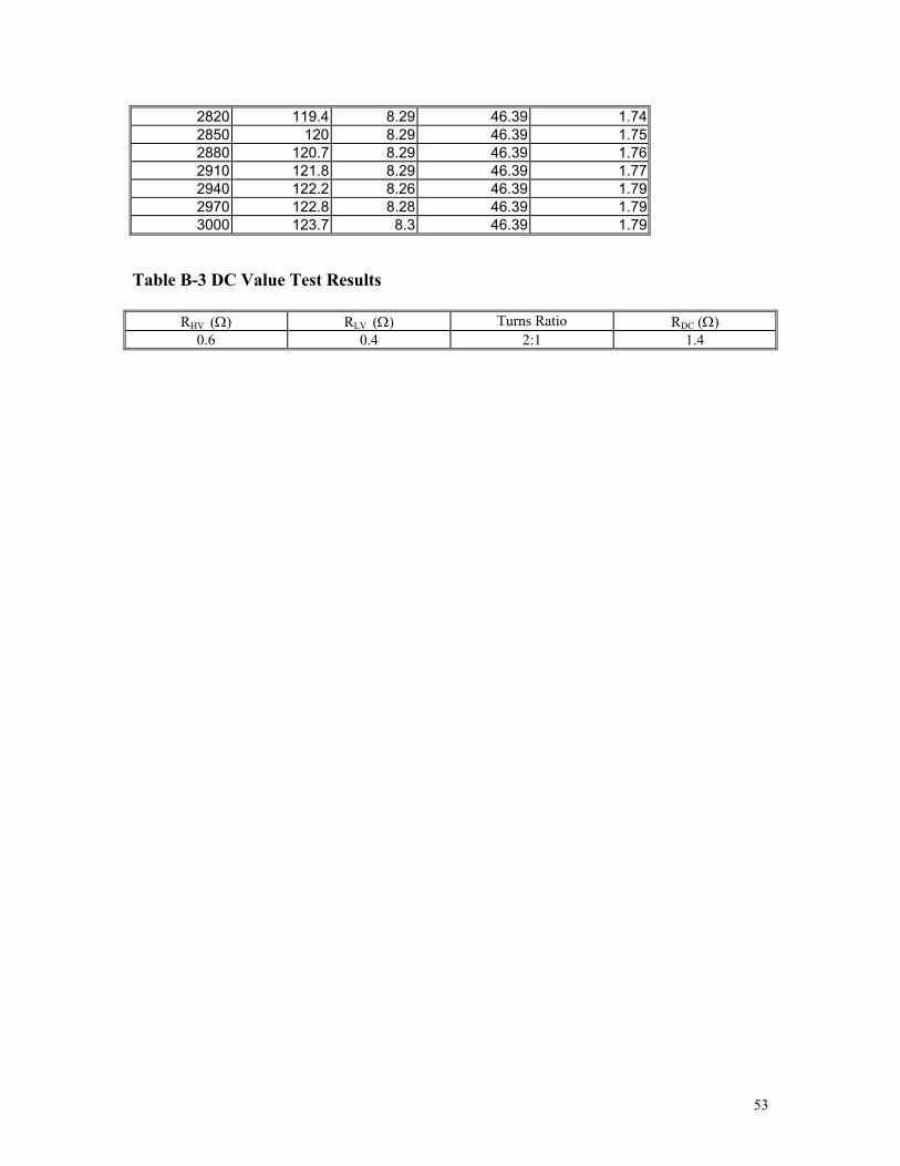
53
2820 119.4 8.29 46.39 1.74 2850 120 8.29 46.39 1.75 2880 120.7 8.29 46.39 1.76 2910 121.8 8.29 46.39 1.77 2940 122.2 8.26 46.39 1.79 2970 122.8 8.28 46.39 1.79 3000 123.7 8.3 46.39 1.79
Table B-3 DC Value Test Results
RHV (Ω) RLV (Ω) Turns Ratio RDC (Ω) 0.6 0.4 2:1 1.4
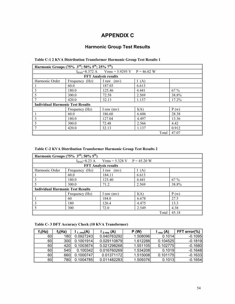
54
APPENDIX C
Harmonic Group Test Results
Table C-1 2 KVA Distribution Transformer Harmonic Group Test Results 1
Harmonic Groups (75% 3nd; 50% 5th; 25% 7th) IRMS=8.372 A Vrms = 5.9295 V P = 46.02 W FFT Analysis results Harmonic Order Frequency (Hz) I raw (mv) I (A) 1 60.0 187.03 6.613 3 180.0 125.46 4.441 67 % 5 300.0 72.58 2.569 38.8% 7 420.0 32.13 1.137 17.2% Individual Harmonic Test Results Frequency (Hz) I raw (mv) I(A) P (w) 1 60.0 186.60 6.606 28.38 3 180.0 127.04 4.497 13.36 5 300.0 72.48 2.566 4.42 7 420.0 32.13 1.137 0.912
Total 47.07
Table C-2 KVA Distribution Transformer Harmonic Group Test Results 2
Harmonic Groups (75% 3nd; 50% 5th) IRMS=8.23 A Vrms = 5.328 V P = 45.20 W FFT Analysis results Harmonic Order Frequency (Hz) I raw (mv) I (A) 1 60.0 184.11 6.613 3 180.0 125.40 4.441 67 % 5 300.0 71.2 2.569 38.8% Individual Harmonic Test Results Frequency (Hz) I raw (mv) I(A) P (w) 1 60 184.0 6.678 27.5 3 180 126.4 4.475 13.3 5 300 72.0 2.549 4.38
Total 45.18
Table C- 3 DFT Accuracy Check (10 KVA Transformer)
f1(Hz) f2(Hz) I 1_rms(A) I 2 rms (A) P (W) I rms (A) FFT error(%)60 180 0.0927243 0.040763292 1.508096 0.1014 -0.109560 300 0.1001914 0.029110879 1.612288 0.104525 -0.181960 420 0.1003674 0.021298268 1.551105 0.102775 -0.168060 540 0.100342 0.016760269 1.534208 0.1019 -0.164860 660 0.1000747 0.01371172 1.515008 0.101175 -0.163360 780 0.1004785 0.011482283 1.509376 0.1013 -0.1654
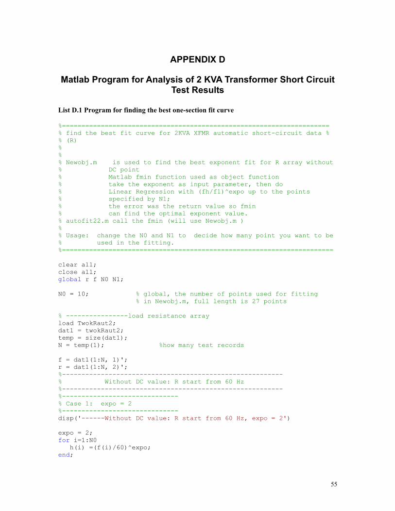
55
APPENDIX D
Matlab Program for Analysis of 2 KVA Transformer Short Circuit Test Results
List D.1 Program for finding the best one-section fit curve %===================================================================== % find the best fit curve for 2KVA XFMR automatic short-circuit data % % (R) % % % Newobj.m is used to find the best exponent fit for R array without % DC point % Matlab fmin function used as object function % take the exponent as input parameter, then do % Linear Regression with (fh/f1)^expo up to the points % specified by N1; % the error was the return value so fmin % can find the optimal exponent value. % autofit22.m call the fmin (will use Newobj.m ) % % Usage: change the N0 and N1 to decide how many point you want to be % used in the fitting. %====================================================================== clear all; close all; global r f N0 N1; N0 = 10; % global, the number of points used for fitting % in Newobj.m, full length is 27 points % ----------------load resistance array load TwokRaut2; dat1 = twokRaut2; temp = size(dat1); N = temp(1); %how many test records f = dat1(1:N, 1)'; r = dat1(1:N, 2)'; %--------------------------------------------------------- % Without DC value: R start from 60 Hz %--------------------------------------------------------- %------------------------------ % Case 1: expo = 2 %------------------------------ disp('------Without DC value: R start from 60 Hz, expo = 2') expo = 2; for i=1:N0 h(i) =(f(i)/60)^expo; end;
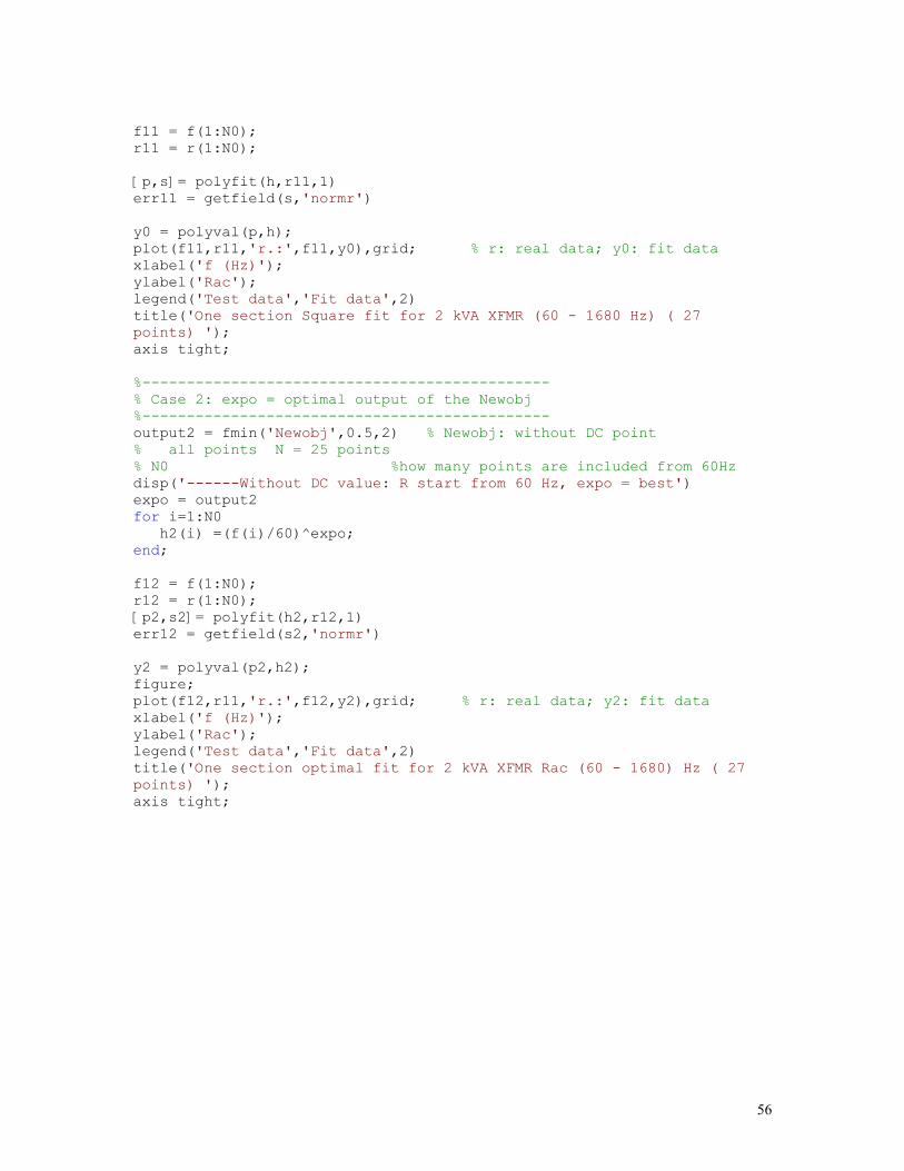
56
f11 = f(1:N0); r11 = r(1:N0); [p,s]= polyfit(h,r11,1) err11 = getfield(s,'normr') y0 = polyval(p,h); plot(f11,r11,'r.:',f11,y0),grid; % r: real data; y0: fit data xlabel('f (Hz)'); ylabel('Rac'); legend('Test data','Fit data',2) title('One section Square fit for 2 kVA XFMR (60 - 1680 Hz) ( 27 points) '); axis tight; %---------------------------------------------- % Case 2: expo = optimal output of the Newobj %---------------------------------------------- output2 = fmin('Newobj',0.5,2) % Newobj: without DC point % all points N = 25 points % N0 %how many points are included from 60Hz disp('------Without DC value: R start from 60 Hz, expo = best') expo = output2 for i=1:N0 h2(i) =(f(i)/60)^expo; end; f12 = f(1:N0); r12 = r(1:N0); [p2,s2]= polyfit(h2,r12,1) err12 = getfield(s2,'normr') y2 = polyval(p2,h2); figure; plot(f12,r11,'r.:',f12,y2),grid; % r: real data; y2: fit data xlabel('f (Hz)'); ylabel('Rac'); legend('Test data','Fit data',2) title('One section optimal fit for 2 kVA XFMR Rac (60 - 1680) Hz ( 27 points) '); axis tight;
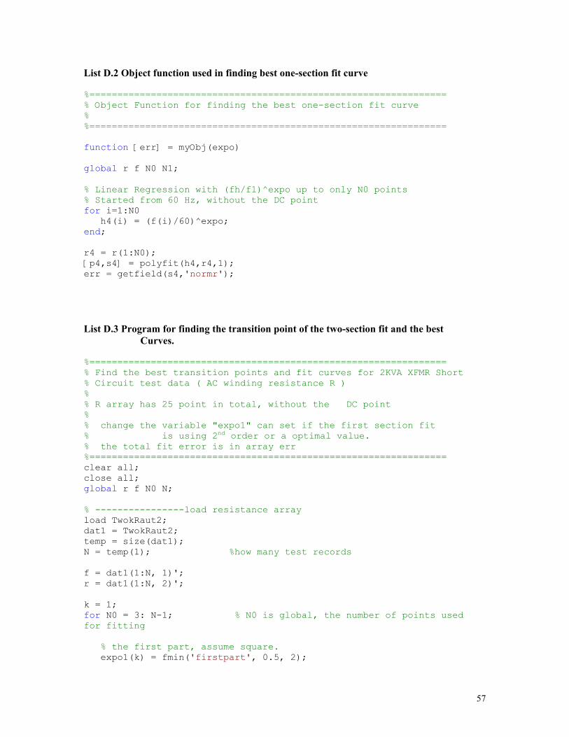
57
List D.2 Object function used in finding best one-section fit curve %================================================================ % Object Function for finding the best one-section fit curve % %================================================================ function [err] = myObj(expo) global r f N0 N1; % Linear Regression with (fh/f1)^expo up to only N0 points % Started from 60 Hz, without the DC point for i=1:N0 h4(i) = (f(i)/60)^expo; end; r4 = r(1:N0); [p4,s4] = polyfit(h4,r4,1); err = getfield(s4,'normr'); List D.3 Program for finding the transition point of the two-section fit and the best Curves. %================================================================ % Find the best transition points and fit curves for 2KVA XFMR Short % Circuit test data ( AC winding resistance R ) % % R array has 25 point in total, without the DC point % % change the variable "expo1" can set if the first section fit % is using 2nd order or a optimal value. % the total fit error is in array err %================================================================ clear all; close all; global r f N0 N; % ----------------load resistance array load TwokRaut2; dat1 = TwokRaut2; temp = size(dat1); N = temp(1); %how many test records f = dat1(1:N, 1)'; r = dat1(1:N, 2)'; k = 1; for N0 = 3: N-1; % N0 is global, the number of points used for fitting % the first part, assume square. expo1(k) = fmin('firstpart', 0.5, 2);
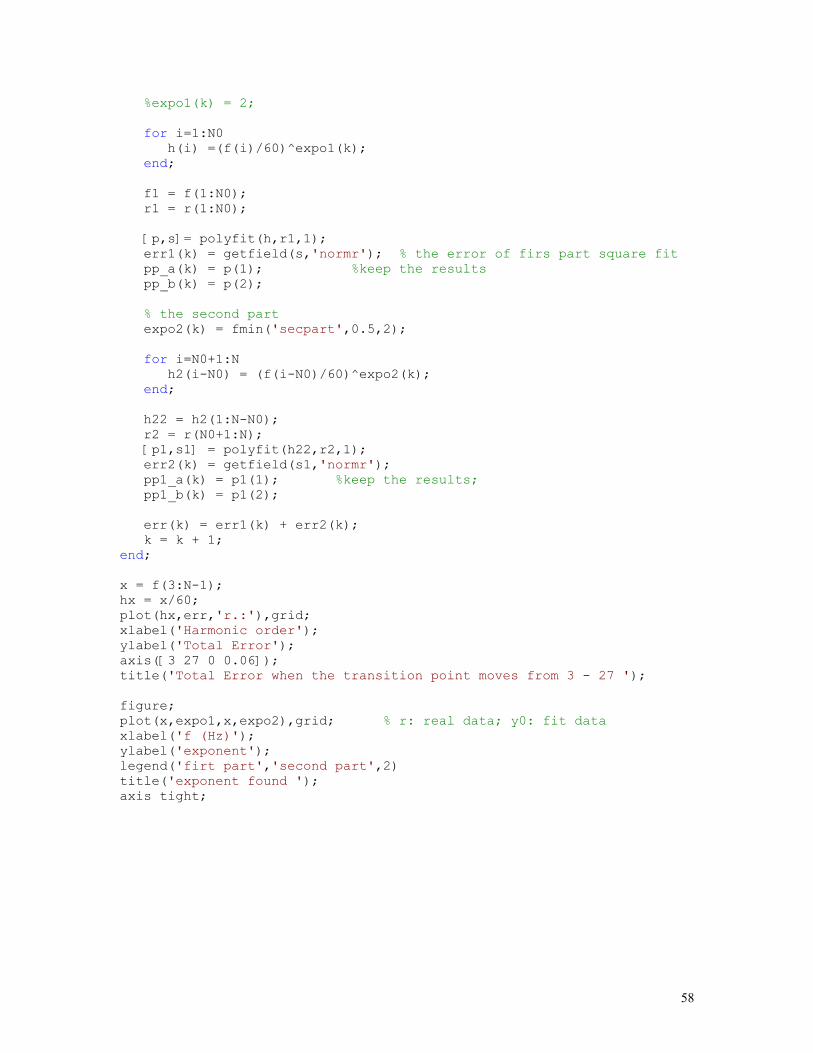
58
%expo1(k) = 2; for i=1:N0 h(i) =(f(i)/60)^expo1(k); end; f1 = f(1:N0); r1 = r(1:N0); [p,s]= polyfit(h,r1,1); err1(k) = getfield(s,'normr'); % the error of firs part square fit pp_a(k) = p(1); %keep the results pp_b(k) = p(2); % the second part expo2(k) = fmin('secpart',0.5,2); for i=N0+1:N h2(i-N0) = (f(i-N0)/60)^expo2(k); end; h22 = h2(1:N-N0); r2 = r(N0+1:N); [p1,s1] = polyfit(h22,r2,1); err2(k) = getfield(s1,'normr'); pp1_a(k) = p1(1); %keep the results; pp1_b(k) = p1(2); err(k) = err1(k) + err2(k); k = k + 1; end; x = f(3:N-1); hx = x/60; plot(hx,err,'r.:'),grid; xlabel('Harmonic order'); ylabel('Total Error'); axis([3 27 0 0.06]); title('Total Error when the transition point moves from 3 - 27 '); figure; plot(x,expo1,x,expo2),grid; % r: real data; y0: fit data xlabel('f (Hz)'); ylabel('exponent'); legend('firt part','second part',2) title('exponent found '); axis tight;
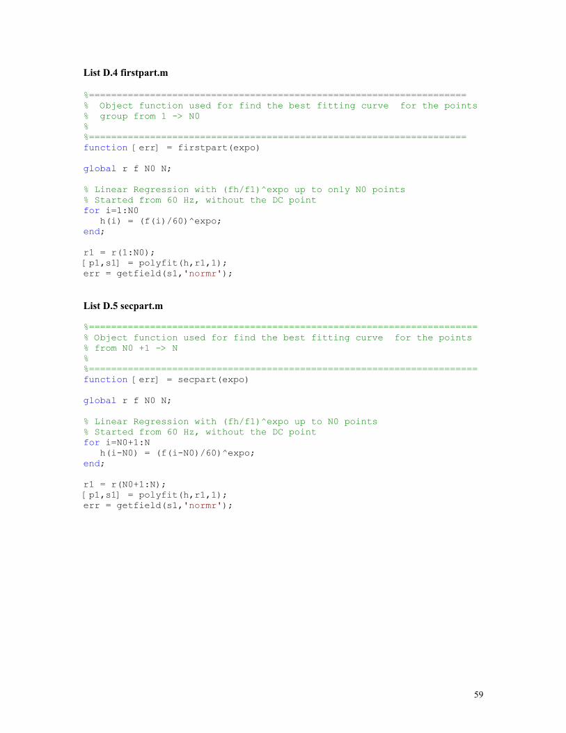
59
List D.4 firstpart.m %==================================================================== % Object function used for find the best fitting curve for the points % group from 1 -> N0 % %==================================================================== function [err] = firstpart(expo) global r f N0 N; % Linear Regression with (fh/f1)^expo up to only N0 points % Started from 60 Hz, without the DC point for i=1:N0 h(i) = (f(i)/60)^expo; end; r1 = r(1:N0); [p1,s1] = polyfit(h,r1,1); err = getfield(s1,'normr'); List D.5 secpart.m %====================================================================== % Object function used for find the best fitting curve for the points % from N0 +1 -> N % %====================================================================== function [err] = secpart(expo) global r f N0 N; % Linear Regression with (fh/f1)^expo up to N0 points % Started from 60 Hz, without the DC point for i=N0+1:N h(i-N0) = (f(i-N0)/60)^expo; end; r1 = r(N0+1:N); [p1,s1] = polyfit(h,r1,1); err = getfield(s1,'normr');

60
APPENDIX E
Matlab Program for Analysis of 10 KVA Transformer Short Circuit Test Results
List E.1 Program for finding the best one-section fit curve %================================================================ % find the best fit for 10 kVA s-c data (R) % the data starts from 60 Hz, 25 points in total % % Newobj.m is used to find the best exponent fit for R array % without DC point % Newobj2.m based on Newobj.m, insert the DC value to the R array % % both used Matlab fmin function as object function % take the exponent as input parameter, then do % Linear Regression with (fh/f1)^expo up to the points % specified by N1; % the error was the return value so fmin % can find the optimal exponent value. % autofit10.m call the fmin (will use Newobj.m and Newobj2.m ) % % case 1: Without DC value ( Newobj.m is used ) % first fit it to square,(so expo is set to =2) % then use the best expo results (the output2) for % fitting % case 2: repeat above 2 tests with DC value inserted at % the head of the number in the R array. % (Newobj2.m is used) % Usage: change the N0 and N1 to decide how many point you want to be % used in the fitting. % % The two files above process the average R value from % dat12_1, dat12_3, dat12_4 and %================================================================ clear all; close all; global r f N0 N1; N0 = 5; % global, the number of points used for fitting % in Newobj.m ( without the DC point) (max = 25 ) N1 = 26; % global, the number of points used for fitting % in Newobj2.m ( with the DC point)(max = 26 ) % ----------------find the average value of r load dat12_1; load dat12_3; load dat12_4; %--------- Data 12_1 dat1 = dat12_1; temp = size(dat1); N = temp(1); %how many test records Hord = dat1(1:N,1)'; %harmonic order f = dat1(1:N,2)'; %frequecy (Hz)
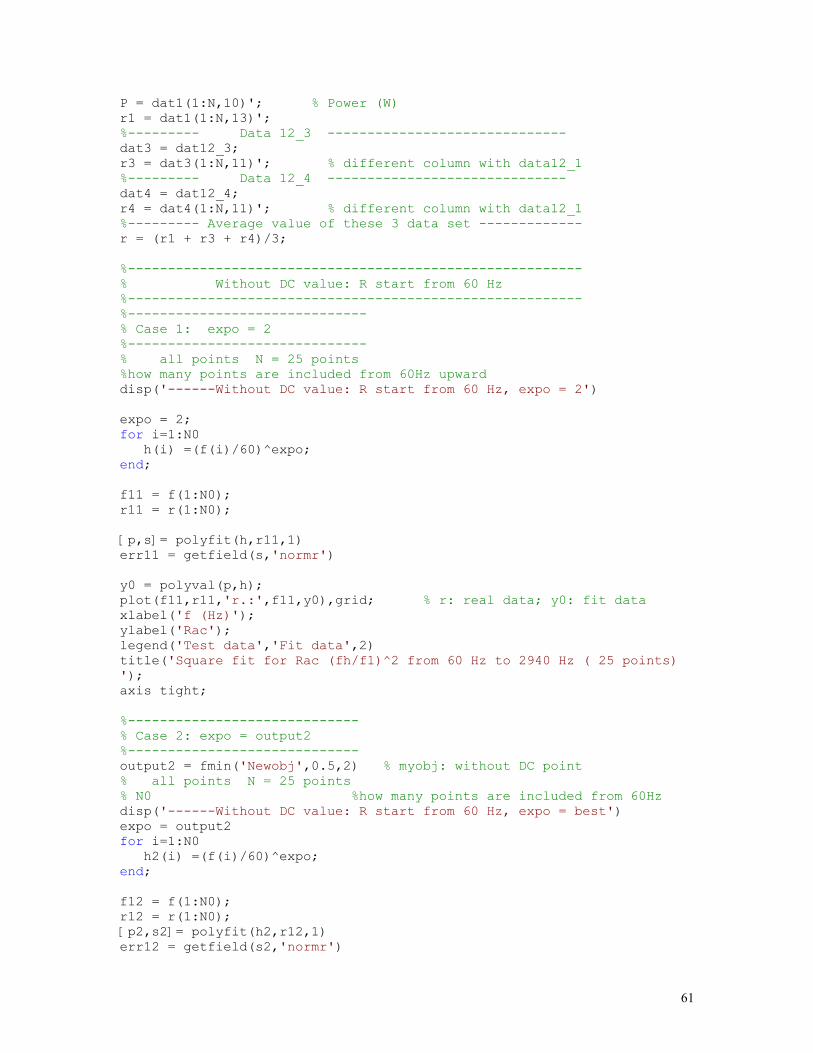
61
P = dat1(1:N,10)'; % Power (W) r1 = dat1(1:N,13)'; %--------- Data 12_3 ------------------------------ dat3 = dat12_3; r3 = dat3(1:N,11)'; % different column with data12_1 %--------- Data 12_4 ------------------------------ dat4 = dat12_4; r4 = dat4(1:N,11)'; % different column with data12_1 %--------- Average value of these 3 data set ------------- r = (r1 + r3 + r4)/3; %--------------------------------------------------------- % Without DC value: R start from 60 Hz %--------------------------------------------------------- %------------------------------ % Case 1: expo = 2 %------------------------------ % all points N = 25 points %how many points are included from 60Hz upward disp('------Without DC value: R start from 60 Hz, expo = 2') expo = 2; for i=1:N0 h(i) =(f(i)/60)^expo; end; f11 = f(1:N0); r11 = r(1:N0); [p,s]= polyfit(h,r11,1) err11 = getfield(s,'normr') y0 = polyval(p,h); plot(f11,r11,'r.:',f11,y0),grid; % r: real data; y0: fit data xlabel('f (Hz)'); ylabel('Rac'); legend('Test data','Fit data',2) title('Square fit for Rac (fh/f1)^2 from 60 Hz to 2940 Hz ( 25 points) '); axis tight; %----------------------------- % Case 2: expo = output2 %----------------------------- output2 = fmin('Newobj',0.5,2) % myobj: without DC point % all points N = 25 points % N0 %how many points are included from 60Hz disp('------Without DC value: R start from 60 Hz, expo = best') expo = output2 for i=1:N0 h2(i) =(f(i)/60)^expo; end; f12 = f(1:N0); r12 = r(1:N0); [p2,s2]= polyfit(h2,r12,1) err12 = getfield(s2,'normr')

62
y2 = polyval(p2,h2); figure; plot(f12,r11,'r.:',f12,y2),grid; % r: real data; y2: fit data xlabel('f (Hz)'); ylabel('Rac'); legend('Test data','Fit data',2) title('Optimal fit for 10 kVA Rac (fh/f1) ^ expo from 60 Hz to 2940 Hz ( 25 points) '); axis tight; %-------------------------------------------------------------- % With DC value: Rdc = 30 ohm, R start from 60 Hz % (total 26 points) % expo = output2 ( the best value fmin found) %-------------------------------------------------------------- % insert the DC point to f, R array rNew(1) = 30; %R dc = 30 Ohm rNew(2:26) = r(1:25); fNew(1) = 0; fNew(2:26) = f(1:25); %---------------------- % Case 1: expo = 2 %---------------------- % Linear Regression with (fh/f1)^2 up to N1 points) %N1 ; f3 = fNew(1:N1); disp('------With DC value: R start from 0 Hz, expo = 2') expo = 2; for i=1:N1 h3(i) = (f3(i)/60)^expo; %use the fit results end; r3 = rNew(1:N1); [p3,s3] = polyfit(h3,r3,1) err21 = getfield(s3,'normr') y3 = polyval(p3,h3); figure; plot(f3,r3,'r.:',f3,y3),grid; xlabel('f (Hz)'); ylabel('Rac'); legend('Test data','Fit data',2) title('Linear regression for Rac (fh/f1)^2 including DC value '); axis tight; %---------------------- % Case 2: expo = output2 %---------------------- output2 = fmin('Newobj2',0.5,2) % myobj2: including DC point % Linear Regression with (fh/f1)^expo up to N1 points % N1
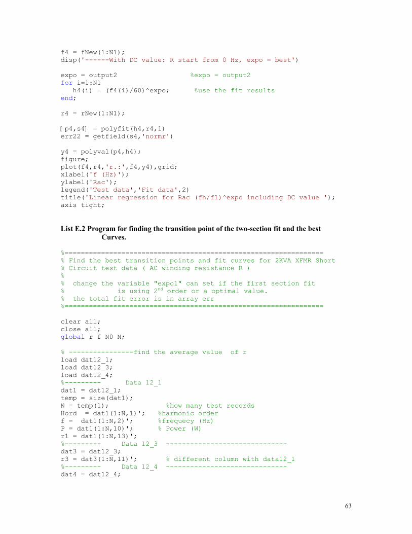
63
f4 = fNew(1:N1); disp('------With DC value: R start from 0 Hz, expo = best') expo = output2 %expo = output2 for i=1:N1 h4(i) = (f4(i)/60)^expo; %use the fit results end; r4 = rNew(1:N1); [p4,s4] = polyfit(h4,r4,1) err22 = getfield(s4,'normr') y4 = polyval(p4,h4); figure; plot(f4,r4,'r.:',f4,y4),grid; xlabel('f (Hz)'); ylabel('Rac'); legend('Test data','Fit data',2) title('Linear regression for Rac (fh/f1)^expo including DC value '); axis tight; List E.2 Program for finding the transition point of the two-section fit and the best Curves. %================================================================ % Find the best transition points and fit curves for 2KVA XFMR Short % Circuit test data ( AC winding resistance R ) % % change the variable "expo1" can set if the first section fit % is using 2nd order or a optimal value. % the total fit error is in array err %================================================================ clear all; close all; global r f N0 N; % ----------------find the average value of r load dat12_1; load dat12_3; load dat12_4; %--------- Data 12_1 dat1 = dat12_1; temp = size(dat1); N = temp(1); %how many test records Hord = dat1(1:N,1)'; %harmonic order f = dat1(1:N,2)'; %frequecy (Hz) P = dat1(1:N,10)'; % Power (W) r1 = dat1(1:N,13)'; %--------- Data 12_3 ------------------------------ dat3 = dat12_3; r3 = dat3(1:N,11)'; % different column with data12_1 %--------- Data 12_4 ------------------------------ dat4 = dat12_4;
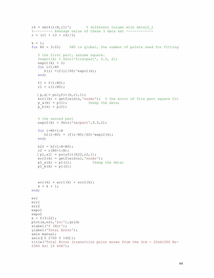
64
r4 = dat4(1:N,11)'; % different column with data12_1 %--------- Average value of these 3 data set ------------- r = (r1 + r3 + r4)/3; k = 1; for N0 = 3:22; %N0 is global, the number of points used for fitting % the first part, assume square. %expo1(k) = fmin('firstpart', 0.5, 2); expo1(k) = 2; for i=1:N0 h(i) =(f(i)/60)^expo1(k); end; f1 = f(1:N0); r1 = r(1:N0); [p,s]= polyfit(h,r1,1); err1(k) = getfield(s,'normr'); % the error of firs part square fit p_a(k) = p(1); %keep the data; p_b(k) = p(2); % the second part expo2(k) = fmin('secpart',0.5,2); for i=N0+1:N h2(i-N0) = (f(i-N0)/60)^expo2(k); end; h22 = h2(1:N-N0); r2 = r(N0+1:N); [p1,s1] = polyfit(h22,r2,1); err2(k) = getfield(s1,'normr'); p1_a(k) = p1(1); %keep the data; p1_b(k) = p1(2); err(k) = err1(k) + err2(k); k = k + 1; end; err err1 err2 expo1 expo2 x = f(3:22); plot(x,err,'ro:'),grid; xlabel('f (Hz)'); ylabel('Total Error'); axis manual; axis([0 2700 0 140]); title('Total Error (transition point moves from the 3rd - 22nd(300 Hz- 2580 Hz) 10 kVA');
65
figure; plot(x,expo1,x,expo2),grid; % r: real data; y0: fit data xlabel('f (Hz)'); ylabel('exponent'); legend('firt part','second part',2) title('exponent found '); axis tight; % find the p, s for the second part best fit N0 = 11; % found for i=N0+1:N h3(i-N0) = (f(i-N0)/60)^expo2(9); end; r1 = r(N0+1:N); [p1,s1] = polyfit(h3,r1,1) errSec = getfield(s1,'normr');

66
APPENDIX F
Instructions for Doing Short Circuit Test Manually Connect Test Device correctly. Please refer to Chapter 3 for different test configuration and connection diagram. Start up the AMX 3120 Power Source • Make sure the Output Power switch of the Master Power source is turned off • Make sure the Output Power switch of the Slave Power source is turned off • Turn on the Input Power switch of the Master Power source • Turn on the Input Power switch of the Slave Power source Start up the Nicolet Pro20 Oscilloscope • Turn on the power switch of Oscilloscope • Set the sweep length to 8192 points under Menu\Acquisition\Sweep length. Refer to
Chapter 3 for detailed explanation of the setting. Start up the AM 503A Current Probe • Turn on the power of the current probe • Degauss the Probe • Set the Currnt/Division setting to 0.5 A/DIV Apply the Voltage to test transformer • Close the switch on the test bench. • On the UPC32 Panel of the AMX 3120 Power Source, choose the correct Voltage and
Frequency or harmonic groups • Turn on the Output Power Enable switch on the UPC32 Panel • Turn on the Output Power switch of the Master Power Source Record the test data • Press Autosetup of the oscilloscope. • Set the Time setting to 200 µs. • Store the data to floppy disk

67
Appendix G
Laboratory Equipment and Computer Resources Test Transformer: (1) 2 KVA single phase, dry type,4 winding 120/240 Volt transformer Square D cat. No. 2S1F (2) 10 KVA amorphous steel core single-phase oil filled distribution transformer 7200-120/240-V Lab Equipment Pacific Source AMX 3120 AC Power Source Nicolet Pro 20S digital oscilloscope Tektronix model AM503S current probe and amplifier Computer Hardware Gateway 2000 486 DX2 66MHz Computer Computer Software Vu-Point II (version 3.14)


![Open Archive TOULOUSE Archive Ouverte (OATAO) · The “Space Product Assurance - Derating - EEE components” ECSS-Q- ST-30-11C [14] specifies electrical derating requirements applicable](https://img.pdfslide.net/doc/110x75/5b9509e309d3f2205c8c0df8/open-archive-toulouse-archive-ouverte-oatao-the-space-product-assurance.jpg)