Physica E 46 (2012) 149–154

Contents lists available at SciVerse ScienceDirect

Physica E

1386-94

http://d

n Corr

E-m

journal homepage: www.elsevier.com/locate/physe

Transient behavior of pulse propagation in a double-quantum-dotAharonov–Bohm interferometer

Roberto Romo a,n, Jorge Villavicencio a, M.L. Ladron de Guevara b

a Facultad de Ciencias, Universidad Autonoma de Baja California, Apartado Postal 1880, 22800 Ensenada, Baja California, Mexicob Departamento de Fısica, Universidad Catolica del Norte, Casilla 1280, Antofagasta, Chile

H I G H L I G H T S

c We analyze a Gaussian pulse scattered by an Aharonov–Bohm interferometer.c A dynamical Fano profile is found traveling embedded in the scattered pulse.c The shape of the scattered pulse is controlled by varying the Aharonov–Bohm phase.c The energy and width of the Fano resonance govern the transients of the packet.c The shape of the scattered wavepacket reveals information of the molecular states.

a r t i c l e i n f o

Article history:

Received 30 March 2012

Accepted 11 September 2012Available online 24 September 2012

77/$ - see front matter & 2012 Elsevier B.V. A

x.doi.org/10.1016/j.physe.2012.09.008

esponding author. Tel.: þ52 646 174 59 25; f

ail address: romo@uabc.edu.mx (R. Romo).

a b s t r a c t

We analyze the transient behavior of a pulse scattered by a double quantum dot Aharonov–Bohm

interferometer. Our study uses the analytical solution of the time-dependent Schrodinger equation for

cutoff Gaussian wavepackets incoming at the system. We find that the wavepacket evolution is

governed by a dynamical Fano profile, which is a transient structure that travels embedded in the

scattered wavepacket, whose shape and time evolution can be controlled by manipulations of the

Aharonov–Bohm phase of the device. We demonstrate analytically that this transient structure is

characterized by the energy and width associated to the Fano resonance. At long times and distances

from the interaction region, the transient oscillatory structures fades away and both the Breit–Wigner

resonance and Fano line-shape are fully imprinted on the Gaussian pulse.

& 2012 Elsevier B.V. All rights reserved.

1. Introduction

The dynamical studies based on the paradigm of wavepacketpropagation, have been traditionally devoted to quantum struc-tures characterized by explicit one-dimensional potentials, andBreit–Wigner type resonances in the transmission characteristics[1–3]. The interest in analyzing Gaussian pulse propagation insystems, whose conductance involves asymmetrical Fano profiles,has arisen only recently [4,5]. These dynamical studies were inpart motivated by the experimental observation of clear Fanoprofiles in the conductance in Aharonov–Bohm (AB) interferom-eters [6] and quantum wires with side-coupled quantum dots[7,8]. In addition to the theoretical and experimental findings inthe stationary conductance, there is a rich physics to explore inthe dynamical aspects of these quantum structures. The above isbased on the premise that the transmitted pulse carries relevantinformation of the system, which manifests itself in the form in

ll rights reserved.

ax: þ52 6461744560.

which the propagating packet evolves from the transient to thelong time regime. Particularly, it has been theoretically shown indifferent systems and initial conditions, that there exists a closelink between the main characteristics of the energy spectrum andthe peculiarities of the transmitted pulse in both the space andtime domains [3,5,9]. This connection between the system spec-trum and the scattering characteristics provides more options forcontrolling the features of the transmitted pulses by a propermanipulation of the system’s parameters. Wulf and Skalozub [4]studied the scattering in a generic one-channel quantum systemwhere a Fano line shape in transmission arises from the inter-ference of a resonant part and a constant background in theamplitude of scattering [10]. They provided an analytical solutionof the problem for an incoming Gaussian pulse when its meanenergy is close to the energy of the resonance. The approach byWulf et al. [4] was used by Malyshev et al. [5] in the scattering ofa pulse by two quantum dots side-attached to a quantum wire,showing the splitting of the electronic wave packet.

In this work, we use the analytical approach based on cutoff

Gaussian wave packets introduced in Ref. [2], to explore the scatteringof electrons by a double quantum dot molecule embedded in an AB

R. Romo et al. / Physica E 46 (2012) 149–154150

interferometer. The transmission spectrum of this system is aconvolution of Breit–Wigner and Fano resonances around the mole-cular energies, the nature and width of each resonance dependingsensitively on the AB phase [11–13]. Our approach allows to dealwith transmission spectra composed of resonances at differentenergies, without imposing any constraints to the mean energy ofthe incident wavepacket. We study how the features of the transmis-sion spectrum are extended on the transmitted time-dependentsolution. In particular we analyze the effects of variations of the ABphase on the evolution of the transmitted pulse in the whole timedomain, from the transient regime to the asymptotic limit of longtimes and distances.

The paper is organized as follows. In Section 2 we present theformal solution of the problem which involves an exact analyticaltime-dependent solution of Schrodinger’s equation for cutoffGaussian wavepackets in a quantum shutter setup. The formalderivation also takes into account explicit formulas of the trans-mission amplitude of the double dot AB interferometer, tðeÞ, inenergy domain, derived from the equation of motion method forthe Green function. Section 3 presents the results, where weanalyze the time evolution of the transmitted pulses and theeffects induced by variations of the AB phase on the Fano profileimprinted on the traveling Gaussian pulse, and a detailed analysisof the transient behavior of the Fano resonances. Finally, inSection 4 we present the conclusions.

2. Model

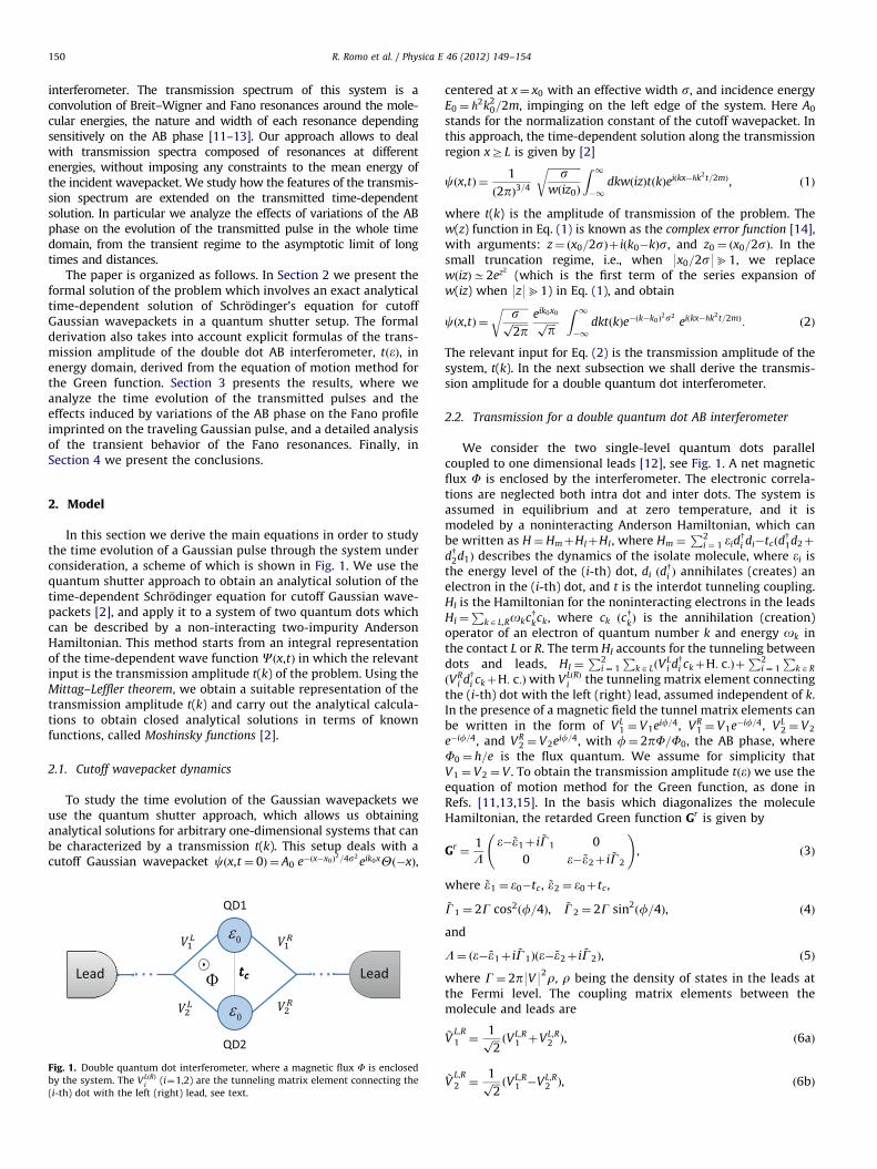
In this section we derive the main equations in order to studythe time evolution of a Gaussian pulse through the system underconsideration, a scheme of which is shown in Fig. 1. We use thequantum shutter approach to obtain an analytical solution of thetime-dependent Schrodinger equation for cutoff Gaussian wave-packets [2], and apply it to a system of two quantum dots whichcan be described by a non-interacting two-impurity AndersonHamiltonian. This method starts from an integral representationof the time-dependent wave function Cðx,tÞ in which the relevantinput is the transmission amplitude t(k) of the problem. Using theMittag–Leffler theorem, we obtain a suitable representation of thetransmission amplitude t(k) and carry out the analytical calcula-tions to obtain closed analytical solutions in terms of knownfunctions, called Moshinsky functions [2].

2.1. Cutoff wavepacket dynamics

To study the time evolution of the Gaussian wavepackets weuse the quantum shutter approach, which allows us obtaininganalytical solutions for arbitrary one-dimensional systems that canbe characterized by a transmission t(k). This setup deals with acutoff Gaussian wavepacket cðx,t¼ 0Þ ¼ A0 e�ðx�x0Þ

2=4s2eik0xYð�xÞ,

Fig. 1. Double quantum dot interferometer, where a magnetic flux F is enclosed

by the system. The VLðRÞi (i¼1,2) are the tunneling matrix element connecting the

(i-th) dot with the left (right) lead, see text.

centered at x¼ x0 with an effective width s, and incidence energyE0 ¼ _2k2

0=2m, impinging on the left edge of the system. Here A0

stands for the normalization constant of the cutoff wavepacket. Inthis approach, the time-dependent solution along the transmissionregion xZL is given by [2]

cðx,tÞ ¼1

ð2pÞ3=4

ffiffiffiffiffiffiffiffiffiffiffiffiffis

wðiz0Þ

r Z 1�1

dkwðizÞtðkÞeiðkx�_k2t=2mÞ, ð1Þ

where t(k) is the amplitude of transmission of the problem. Thew(z) function in Eq. (1) is known as the complex error function [14],with arguments: z¼ ðx0=2sÞþ iðk0�kÞs, and z0 ¼ ðx0=2sÞ. In thesmall truncation regime, i.e., when 9x0=2s9b1, we replacewðizÞC2ez2

(which is the first term of the series expansion ofw(iz) when 9z9b1) in Eq. (1), and obtain

cðx,tÞ ¼

ffiffiffiffiffiffiffiffiffiffisffiffiffiffiffiffi2pp

reik0x0ffiffiffiffipp

Z 1�1

dktðkÞe�ðk�k0Þ2s2

eiðkx�_k2t=2mÞ: ð2Þ

The relevant input for Eq. (2) is the transmission amplitude of thesystem, t(k). In the next subsection we shall derive the transmis-sion amplitude for a double quantum dot interferometer.

2.2. Transmission for a double quantum dot AB interferometer

We consider the two single-level quantum dots parallelcoupled to one dimensional leads [12], see Fig. 1. A net magneticflux F is enclosed by the interferometer. The electronic correla-tions are neglected both intra dot and inter dots. The system isassumed in equilibrium and at zero temperature, and it ismodeled by a noninteracting Anderson Hamiltonian, which canbe written as H¼HmþHlþHI , where Hm ¼

P2i ¼ 1 eid

y

i di�tcðdy

1d2þ

dy2d1Þ describes the dynamics of the isolate molecule, where ei isthe energy level of the (i-th) dot, di ðd

y

i Þ annihilates (creates) anelectron in the (i-th) dot, and t is the interdot tunneling coupling.Hl is the Hamiltonian for the noninteracting electrons in the leadsHl ¼

PkAL,Rokcykck, where ck ðc

y

kÞ is the annihilation (creation)operator of an electron of quantum number k and energy ok inthe contact L or R. The term HI accounts for the tunneling betweendots and leads, HI ¼

P2i ¼ 1

PkA LðV

Li dyi ckþH: c:Þþ

P2i ¼ 1

PkAR

ðVRi dyi ckþH: c:Þwith VLðRÞ

i the tunneling matrix element connectingthe (i-th) dot with the left (right) lead, assumed independent of k.In the presence of a magnetic field the tunnel matrix elements canbe written in the form of VL

1 ¼ V1eif=4, VR1 ¼ V1e�if=4, VL

2 ¼ V2

e�if=4, and VR2 ¼ V2eif=4, with f¼ 2pF=F0, the AB phase, where

F0 ¼ h=e is the flux quantum. We assume for simplicity thatV1 ¼ V2 ¼ V . To obtain the transmission amplitude tðeÞ we use theequation of motion method for the Green function, as done inRefs. [11,13,15]. In the basis which diagonalizes the moleculeHamiltonian, the retarded Green function Gr is given by

Gr¼

1

Le�~e1þ i ~G1 0

0 e�~e2þ i ~G2

!, ð3Þ

where ~e1 ¼ e0�tc , ~e2 ¼ e0þtc ,

~G1 ¼ 2G cos2ðf=4Þ, ~G2 ¼ 2G sin2ðf=4Þ, ð4Þ

and

L¼ ðe�~e1þ i ~G1Þðe�~e2þ i ~G2Þ, ð5Þ

where G¼ 2p9V92r, r being the density of states in the leads atthe Fermi level. The coupling matrix elements between themolecule and leads are

~VL,R

1 ¼1ffiffiffi2p ðVL,R

1 þVL,R2 Þ, ð6aÞ

~VL,R

2 ¼1ffiffiffi2p ðVL,R

1 �VL,R2 Þ, ð6bÞ

R. Romo et al. / Physica E 46 (2012) 149–154 151

where VL,R1,2 ¼ VL,R

1,2ðfÞ are the given above. The transmission ampli-tude can be deduced from the electron retarded Green functionfrom the relation [16]

tðeÞ ¼Xn,m

VR

nGrn,mðeÞV

Ln

m , ð7Þ

where VLðRÞ

n ¼ ½2rLðRÞ�1=2 ~V

LðRÞ

n , with ~VLðRÞ

n the coupling matrix ele-ments between the n-th molecular state and the left (right) leadand rLðRÞ the density of states in the left (right) lead at the Fermienergy. After evaluating Eq. (7) we obtain

tðeÞ ¼~G1

e�~e1þ i ~G1

�~G2

e�~e2þ i ~G2

, ð8Þ

and consequently the transmission probability is,

TðeÞ ¼ 9tðeÞ92¼

½ ~G2ðe�~e1Þ�~G1ðe�~e2Þ�

2

½ ~G2

1þðe�~e1Þ2�½ ~G

2

2þðe�~e2Þ2�

: ð9Þ

In order to properly evaluate the integral given by Eq. (2), thetransmission amplitude must be given as a function of k. There-fore we introduce the following definitions

En ¼2m

_2~en, wn ¼

2m

_2~Gn, ð10Þ

and the transmission becomes

tðkÞ ¼w1

k2�E1þ iw1

�w2

k2�E2þ iw2

, ð11Þ

where we have used e¼ _2k2=2m. We rewrite the above expres-sion by decomposing each of the terms into partial fractions byusing the Mittag–Leffler theorem [17]. This results in

tðkÞ ¼1

2½z1f 1ðkÞ�z2f 2ðkÞ�, ð12Þ

where

f nðkÞ ¼1

k�knþ iUn�

1

k�kn�iUnð13Þ

and

zn ¼wn

kn�iUn, ð14Þ

with

kn ¼1ffiffiffi2p ½ðE2

nþw2nÞ

1=2þEn�

1=2, ð15aÞ

Un ¼1ffiffiffi2p ½ðE2

nþw2nÞ

1=2�En�

1=2: ð15bÞ

2.3. Dynamical solution for a cutoff wavepacket in a double dot AB

interferometer

Inserting in Eq. (2) the transmission t(k) given by Eqs.(12)–(15), and using the identity

i

2p

Z 1�1

dxeixx0 e�ix2t0_=2m

x�k0¼

Mðx0,k0,t0Þ; Imðk0Þo0,

�Mð�x0,�k0,t0Þ; Imðk0Þ40,

(ð16Þ

where

Mðx00,k00,t00Þ ¼1

2eimx002=2_t00

wðiy00Þ ð17Þ

is the Moshinsky function, with

y00 ¼ e�ip=4

ffiffiffiffiffiffiffiffiffiffim

2_t00

rx00�

_k00

mt00

� �, ð18Þ

leads to the following expression for the scattered wave function

cðx,tÞ ¼ eiðk0x�_k20t=2mÞ

X2

n ¼ 1

~zn½Mðy�n ÞþMðyþn Þ�, ð19Þ

where ~zn ¼ ð�1Þniðsp=ffiffiffiffiffiffi2ppÞ1=2zn, and

Mðy7n Þ ¼

1

2eimX02=2_T 0wðiy7

n Þ ð20Þ

is the Moshinsky function, with

y7n ðx,tÞ ¼ e�ip=4

ffiffiffiffiffiffiffiffiffiffim

2_T 0

r8X07

_Q 7n

mT 0

� �, ð21Þ

where

Q 7n ¼�k08kn7 iUn, ð22aÞ

X0 ¼ x�x0�v0t, ð22bÞ

T 0 ¼ t�it, ð22cÞ

with v0 ¼ _k0=m, and t¼ 2ms2=_.

2.4. Asymptotic formula

In this subsection we analyze the behavior of the wavefunctionat long times and distances with the stationary-phase approx-imation. We begin from the integral representation of the time-dependent solution given by Eq. (2). According to the stationary-phase method [18], the major contribution to the integral (2)arises from the vicinity of those points at which the phasefðkÞ � ðkx�_k2t=2mÞ is stationary, i.e., f0ðkÞ ¼ dfðkÞ=dk¼ 0; inour case the stationary point is given by ks ¼mðx�x0Þ=_t. Theintegral can be evaluated explicitly to yield

casyðx,tÞ ¼

ffiffiffiffiffiffiffiffiffiffisffiffiffiffiffiffi2pp

reik0x0ffiffiffiffipp

2p9f00ðksÞ9

" #1=2

tðksÞe�ðk�k0Þ

2s2

ei½fðksÞ�p=4�: ð23Þ

From the above equation, we observe that the correspondingprobability density is proportional to the transmission coefficient,i.e., 9casyðx,tÞ92

p9tðksÞ92¼ TðksÞ. It is clear from this expression

that when the asymptotic regime is reached, the main features ofthe transmission coefficient observed in k-space are now mappedinto the spatial regime by means of the correspondence k-ks. Therelationship between some features of the transmission spectra inthe time dependent transmitted wave function has been noticedearlier using cutoff plane waves in superlattices [9], and recentlyin wavepacket scattering [3,5].

3. Results

The following analysis is centered in the role of the AB phaseon the spatial and temporal evolution of the transmitted packet,and namely in the behavior of the transient associated with theFano line shape of the transmission, a characteristic signature ofthese kind of systems.

3.1. Wavepacket dynamics and the effect of variations of the AB

phase

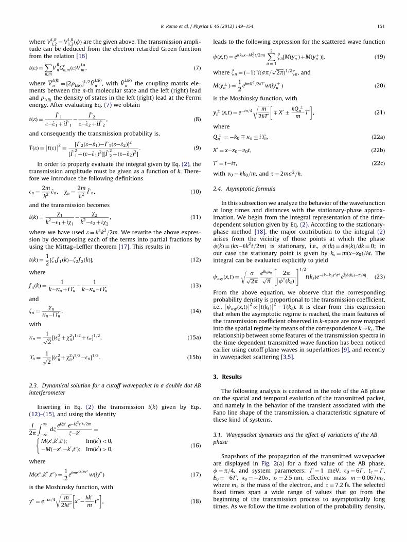
Snapshots of the propagation of the transmitted wavepacketare displayed in Fig. 2(a) for a fixed value of the AB phase,f¼ p=4, and system parameters: G¼ 1 meV, E0 ¼ 6G, tc ¼G,E0 ¼ 6G, x0 ¼�20s, s¼ 2:5 nm, effective mass m¼ 0:067me,where me is the mass of the electron, and t¼ 7:2 fs. The selectedfixed times span a wide range of values that go from thebeginning of the transmission process to asymptotically longtimes. As we follow the time evolution of the probability density,

0.000

0.007

0.014t=102τ

0.00

0.01

0.02 t=103τ

0.00

0.01

0.02 t=104τ

|Ψ|2

0.00

0.01

0.02t=105τ

0.0 0.2 0.4 0.6 0.8 1.00.00

0.01

0.02t=106τ

χ

0.0 4.0 8.0 12.00.0

0.5

1.0

T

ε

0.000

0.005

0.010 t=102τ

0.00

0.01

0.02t=103τ

0.00

0.01

0.02t=104τ

|Ψ|2

0.00

0.01

0.02t=105τ

0.0 0.2 0.4 0.6 0.8 1.0

0.00

0.01

0.02t=106τ

χ

0.000

0.005

0.010 t=102τ

0.00

0.01

0.02t=103τ

0.00

0.01

0.02t=104τ

|Ψ|2

0.00

0.01

0.02t=105τ

0.0 0.2 0.4 0.6 0.8 1.00.000

0.008

0.016t=106τ

χ

0.0 4.0 8.0 12.00.0

0.5

1.0

T

ε

Fig. 2. Normalized probability density 9C92¼ 9c92

ffiffiffiffiffiffiffiffiffiffiffiffiffiffiffiffiffiffiffiffi1þðt=tÞ2

qas a function of the distance w¼ x=ðs

ffiffiffiffiffiffiffiffiffiffiffiffiffiffiffiffiffiffiffiffi1þðt=tÞ2

qÞ at different times, for different values the AB phase:

(a) f¼ p=4, (b) f¼ p, and (c) f¼ 7p=4. In cases (a) and (c) the asymptotic probability density from Eq. (24) (red dotted line) is included for comparison, and the insets

show the transmission coefficient T of the system. In case (b) we consider two cases corresponding to tc ¼G (solid line) and tc ¼ 2G (blue dashed line). (For interpretation

of the references to color in this figure caption, the reader is referred to the web version of this article.)

R. Romo et al. / Physica E 46 (2012) 149–154152

i.e., downward direction in panel (a) of Fig. 2, we can appreciatethe dramatic deformations experienced by the packet as itpropagates along the transmission region. As a result of thescattering, the shape of the packet looks quite irregular at thefirst stages, and, as time goes on, a reshaping process occurs onthe transmitted packet in such a way that it gradually tends toadopt a stable form that resembles the transmission coefficientprofile (compare the graph at the bottom with the inset).

The temporary trapped k-components of the incident wave-packet participate in the building up of the quasi-stationary states atthe molecular energies, and are released as these states decay out ofthe system at a rate established by the corresponding lifetimes. As aconsequence, the interferometer acts as a filter that separates in thespatial domain the characteristic features associated to each reso-nance. At the early stages, the deformation of the packet observed inFig. 2(a) is in part with the result of a mixture of the decay productsof both molecular resonances. The broader (Breit–Wigner) reso-nance is quickly released by the system and hence is the first onethat is reconstructed in the traveling transmitted wavepacket. As wecan see in Fig. 2(a), this occurs at approximately t� 104t, andappears as a broad peak centered at w¼ 0:47, while the oscillatingtransient associated to the sharper (Fano) resonance appears super-imposed on this broad peak. More time is required for the fullreconstruction of the latter due to its smaller resonance width, andthe corresponding Fano profile appears completely formed atw¼ 0:56 (after t� 106t).

For the same system parameters and wavepacket initial con-dition, Figs. 2(b,c) show the time and spatial evolution of thetransmitted packet for f¼ p and f¼ 7p=4, respectively. In con-trast to the case f¼ p=4, the situation with AB phase f¼ p doesnot fulfill the conditions for the formation of the Fano profilesince the transmission coefficient is symmetrical [12]. Theabsence of Fano characteristic is also evident in the transmittedpacket as is clearly shown in all graphs of Fig. 2(b). Here, we usedtwo values of the interdot coupling tc ¼G (solid line), and tc ¼ 2G(red dashed line), in the latter case the two resonances are betterresolved. In both cases, the wavepacket evolves quickly to the

stationary situation, in comparison with the case f¼ p=4, due tothe fact that the involved resonances are broad and have rela-tively short lifetimes.

In the case f¼ 7p=4, the asymmetry of the conductanceguarantees the formation of a Fano profile. This occurs with theroles of the molecular resonances inverted with respect tothe case f¼ p=4, in such a way that now the Fano line appearson the left of the Breit–Wigner resonance in the transmissioncoefficient (see inset at the bottom of panel (c) of Fig. 2). Bysimple visual comparison with the case f¼ p=4, we note that thetransmitted wavepacket follows a similar evolution, also with areshaping that leads to a profile similar to the correspondingtransmission coefficient. In both cases of Fig. 2(a,c), the buildingup of the Fano profile is characterized by a transient that appearsas a damped oscillatory pattern. For asymptotically long times,these oscillating transients disappear, as shown in the bottom ofpanels (a) and (c) of Fig. 2, where the wavepackets adopt theshape of the corresponding transmission coefficient. This isconsistent with the asymptotic formula of the probability density,obtained as the square modulus of Eq. (23), namely

9casyðx,tÞ92¼

ffiffiffiffi2

p

r1

stt

e�2ðks�k0Þ2s2

Tmðx�x0Þ

_t

� �, ð24Þ

where we note that the transmission coefficient T, instead of beinga function of the incidence energy E, it appears in the aboveexpression as a position-dependent function. This clearly showshow the spectrum is mapped into the spatial domain, and explainswhy the shape of the transmitted packet adopts the form of thetransmission coefficient at asymptotically long times. For the sakeof comparison, we included in the bottom of panels (a) and (c) ofFig. 2 (t� 106t) the calculation of 9casyðx,tÞ92

(Eq. (24)) (red dottedlines), and it perfectly agrees with the calculation of 9cðx,tÞ92

withthe exact solution, given by Eq. (19) (solid line).

A clear picture of the effect of the AB phase f on the overallbehavior of the transmitted wave packet can be observed follow-ing the plots of Fig. 2 from left to right at the desired fixed time.For 0ofop the Fano characteristic travels in an advanced

R. Romo et al. / Physica E 46 (2012) 149–154 153

position relative to the main body of the packet, and for pofo2p it travels is delayed. The above means that, an hypothe-tical detector placed at a fixed position would could provide uswith information about the AB phase of the device through ameasurement performed outside the system.

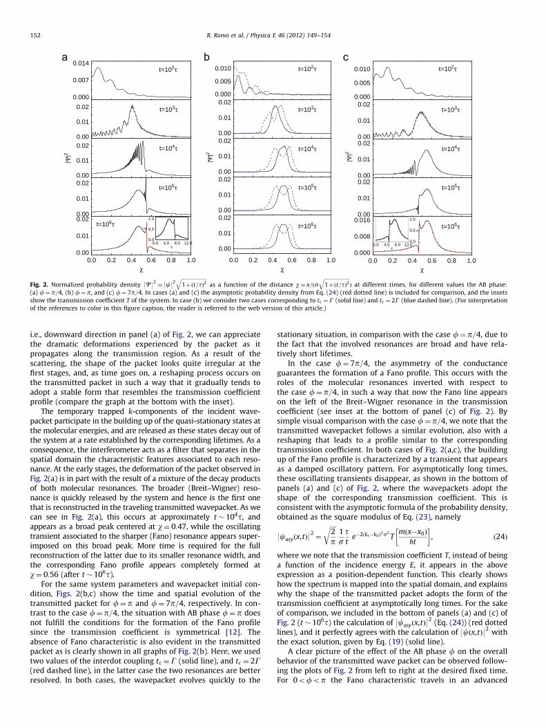
3.2. Analysis of the transient

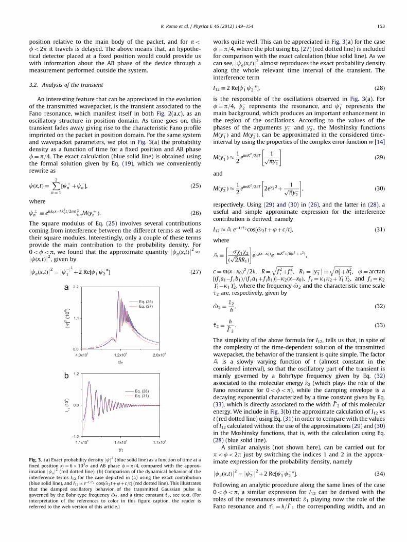
An interesting feature that can be appreciated in the evolutionof the transmitted wavepacket, is the transient associated to theFano resonance, which manifest itself in both Fig. 2(a,c), as anoscillatory structure in position domain. As time goes on, thistransient fades away giving rise to the characteristic Fano profileimprinted on the packet in position domain. For the same systemand wavepacket parameters, we plot in Fig. 3(a) the probabilitydensity as a function of time for a fixed position and AB phasef¼ p=4. The exact calculation (blue solid line) is obtained usingthe formal solution given by Eq. (19), which we convenientlyrewrite as

cðx,tÞ ¼X2

n ¼ 1

½cþn þc�

n �, ð25Þ

where

c7n � eiðk0x�_k2

0t=2mÞ ~znMðy7n Þ: ð26Þ

The square modulus of Eq. (25) involves several contributionscoming from interference between the different terms as well astheir square modules. Interestingly, only a couple of these termsprovide the main contribution to the probability density. For0ofop, we found that the approximate quantity 9caðx,tÞ92

�

9cðx,tÞ92, given by

9caðx,tÞ92¼ 9c�9

2

1 þ2 Re½c�1 c�n

2 � ð27Þ

Fig. 3. (a) Exact probability density 9c92(blue solid line) as a function of time at a

fixed position xf ¼ 6� 103s and AB phase f¼p=4, compared with the approx-

imation 9ca92

(red dotted line). (b) Comparison of the dynamical behavior of the

interference terms I12 for the case depicted in (a) using the exact contribution

(blue solid line), and I12pe�t= ~t2 cos½ ~o2tþjþc=t� (red dotted line). This illustrates

that the damped oscillatory behavior of the transmitted Gaussian pulse is

governed by the Bohr type frequency ~o2, and a time constant ~t2, see text. (For

interpretation of the references to color in this figure caption, the reader is

referred to the web version of this article.)

works quite well. This can be appreciated in Fig. 3(a) for the casef¼ p=4, where the plot using Eq. (27) (red dotted line) is includedfor comparison with the exact calculation (blue solid line). As wecan see, 9caðx,tÞ92

almost reproduces the exact probability densityalong the whole relevant time interval of the transient. Theinterference term

I12 � 2 Re½c�1 c�

2n�, ð28Þ

is the responsible of the oscillations observed in Fig. 3(a). Forf¼ p=4, c�2 represents the resonance, and c�1 represents themain background, which produces an important enhancement inthe region of the oscillations. According to the values of thephases of the arguments y�1 and y�2 , the Moshinsky functionsMðy�1 Þ and Mðy�2 Þ, can be approximated in the considered time-interval by using the properties of the complex error function w [14]

Mðy�1 Þ �1

2eimX2=2_T 1ffiffiffiffi

pp

y�1

" #ð29Þ

and

Mðy�2 Þ �1

2eimX2=2_T 2ey�

22þ

1ffiffiffiffipp

y�2

" #, ð30Þ

respectively. Using (29) and (30) in (26), and the latter in (28), auseful and simple approximate expression for the interferencecontribution is derived, namely

I12 �A e�t= ~t2 cos½ ~o2tþjþc=t�, ð31Þ

where

A��sw1w2

ðffiffiffi2p

RR1Þ

" #eg2ðx�x0Þe�mX2t=_ðt2þt2Þ,

c¼mðx�x0Þ2=2_, R¼

ffiffiffiffiffiffiffiffiffiffiffiffiffiffif 2

r þ f 2i

q, R1 ¼ 9y�1 9�

ffiffiffiffiffiffiffiffiffiffiffiffiffiffiffia2

1þb21

q, j¼ arctan

½ðf ia1�f rb1Þ=ðf ra1þ f ib1Þ��k2ðx�x0Þ, f r ¼ k1k2þU1U2, and f i ¼ k2

U1�k1U2, where the frequency ~o2 and the characteristic time scale~t2 are, respectively, given by

~o2 ¼~e2

_, ð32Þ

~t2 ¼_~G2

: ð33Þ

The simplicity of the above formula for I12, tells us that, in spite ofthe complexity of the time-dependent solution of the transmittedwavepacket, the behavior of the transient is quite simple. The factorA is a slowly varying function of t (almost constant in theconsidered interval), so that the oscillatory part of the transient ismainly governed by a Bohr’type frequency given by Eq. (32)associated to the molecular energy ~e2 (which plays the role of theFano resonance for 0ofop), while the damping envelope is adecaying exponential characterized by a time constant given by Eq.(33), which is directly associated to the width ~G2 of this molecularenergy. We include in Fig. 3(b) the approximate calculation of I12 vst (red dotted line) using Eq. (31) in order to compare with the valuesof I12 calculated without the use of the approximations (29) and (30)in the Moshinsky functions, that is, with the calculation using Eq.(28) (blue solid line).

A similar analysis (not shown here), can be carried out forpofo2p just by switching the indices 1 and 2 in the approx-imate expression for the probability density, namely

9caðx,tÞ92¼ 9c�2 9

2þ2 Re½c�1 c

�

2n�: ð34Þ

Following an analytic procedure along the same lines of the case0ofop, a similar expression for I12 can be derived with theroles of the resonances inverted: ~e1 playing now the role of theFano resonance and ~t1 ¼ _= ~G1 the corresponding width, and an

R. Romo et al. / Physica E 46 (2012) 149–154154

excellent description of the transient associated to the casedisplayed in panel (c) of Fig. 2 can also be accomplished.

4. Conclusions

A formal solution for scattering of cutoff Gaussian wavepacketsthrough an AB interferometer with two coupled quantum dots wasused to perform an analysis of the transient behavior of transmittedwavepackets produced by the molecular states of the system. Weanalyzed the effects of variations of the AB phase at various stages ofthe time-evolution of the scattered wavepacket, and found that theGaussian pulse evolution is governed by a dynamical Fano profile,which strongly depends on the asymmetry of the transmissioncoefficient, where the latter can be controlled by properly manip-ulating the AB phase. Our analysis was performed in the whole timedomain, where we have identified essentially two regimes: theasymptotic (steady state) and transient regime. In the transientregime, the probability density exhibits a traveling damped oscilla-tory structure characterized by a time constant tFano ¼

~G2=_, and aBohr’type frequency ~o2 ¼ ~e2=_, where ~o2, and ~G2 are, respectively,the energy and width of the Fano (or the narrower) resonance. In theasymptotic regime we have demonstrated analytically, using thestationary-phase method, that the probability density of the trans-mitted wavepacket is proportional to the transmission coefficient,i.e., 9cðx,tÞ92

pTðksÞ with ks ¼mðx�x0Þ=_t, which means that thetransmission spectrum is mapped into the time-space domain. Theabove explains why the shape of the transmission coefficient is fullyimprinted on the transmitted Gaussian wavepacket at very largevalues of distance and time. Our results show that, depending on thevalue of the AB phase, an hypothetical detector placed at a fixedposition would register the passage of the dynamical Fano profileretarded or advanced with respect to the main body of the wave-packet. The above could be useful for example as a mechanism tocharacterize the spin–orbit interaction in the molecule through ameasurement of the transmitted spin-polarized current far awayfrom the system, since the Rashba phase and the AB phase can betreated on the same footing of in these kind of systems [19,20].

Acknowledgments

R.R. and J.V. acknowledge financial support of Facultad deCiencias UABC under grant P/PIFI 2011-02MSU0020A-08; R.R. also

thanks the Physics Department of the UCN for their generoussupport during his stays in Antofagasta. This work was alsosupported by Grant Fondecyt 1080660. M.L.L.deG. thanks P.A.Orellana for useful suggestions, and Facultad de Ciencias of UABCfor its hospitality during her stays in Ensenada.

References

[1] L.A. MacColl, Physical Review 40 (1932) 621;H.M.S.A. Goldberg, J.L. Schwartz, American Journal of Physics 35 (1967) 117;T.E. Hartman, Journal of Applied Physics 33 (1962) 3427;J.A. Støvneng, E.H. Hauge, Physical Review B 44 (1991) 13582;S.L. Konsek, T.P. Pearsall, Physical Review B 67 (2003) 045306;Y.G. Peisakhovich, A.A. Shtygashev, Physical Review B 77 (2008) 075327;S.B.A.L. Perez Prieto, J.G. Muga, Journal of Physics A 36 (2003) 2371;M.A. Andreata, V. Dodonov, Journal of Physics A 37 (2004) 2423;E. Granot, A. Marchewka, Journal of Physics A 76 (2007) 012708.

[2] J. Villavicencio, R. Romo, E. Cruz, Physical Review A 75 (2007) 012111.[3] S. Cordero, G. Garcıa-Calderon, Journal of Physics A: Mathematical and

Theoretical 43 (2010) 185301.[4] U. Wulf, V.V. Skalozub, Physical Review B 72 (2005) 165331.[5] A.V. Malyshev, P.A. Orellana, F. Domınguez-Adame, Physical Review B 74

(2006) 033308.[6] K. Kobayashi, H. Aikawa, S. Katsumoto, Y. Iye, Physical Review Letters 88

(2002) 256806;K. Kobayashi, H. Aikawa, S. Katsumoto, Y. Iye, Physical Review B 68 (2003)235304.

[7] K. Kobayashi, H. Aikawa, A. Sano, S. Katsumoto, Y. Iye, Physical Review B 70(2004) 035319.

[8] A.C. Johnson, C.M. Marcus, M.P. Hanson, A.C. Gossard, Physical Review Letters93 (2004) 106803.

[9] J. Villavicencio, R. Romo, Physical Review B 68 (2003) 153311.[10] E.R. Racec, U. Wulf, Physical Review B 64 (2001) 115318.[11] K. Kang, S.Y. Cho, Journal of Physics: Condensed Matter 16 (2004) 117.[12] P.A. Orellana, M.L. Ladron de Guevara, F. Claro, Physical Review B 70 (2004)

233315.[13] Z.M. Bai, M.F. Yang, Y.C. Chen, Journal of Physics: Condensed Matter 16

(2004) 2053.[14] M. Abramowitz, I.A. Stegun, Handbook of Mathematical Functions, Dover,

New York, 1964, p. 297.[15] M.L. Ladron de Guevara, F. Claro, P.A. Orellana, Physical Review B 67 (2003)

195335.[16] T.S. Kim, S. Hershfield, Physical Review B 67 (2003) 235330.[17] M.J. Ablowitz, A.S. Fokas, Complex Variables: Introduction and Applications,

2nd ed., Cambridge University Press, Cambridge, 2003, p. 166.[18] N. Bleinstein, R.A. Handelsman, Asymptotic Expansions of Integrals, Dover,

New York, 1986, p. 219;E. Erdelyi, Asymptotic Expansions, Dover, New York, 1956, p. 51.

[19] C. Feng, J.L. Liu, L.L. Sun, Journal of Applied Physics 101 (2007) 093704.[20] S. Quing-feng, J. Wang, H. Guo, Physical Review B 71 (2005) 165310.