Embed Size (px)
Citation preview

Transient behaviour in a BWR with HafniumCladding
Feasibility study of using BWRs as Higher Actinide Burners at the Example ofRinghals I
SEBASTIAN RAUB
Master of science thesisDivision of Reactor Physics
Royal Institute of TechnologyStockholm, Sweden
TRITA-FYS 2011:36


iii
Abstract
Transmutation of transuranic elements is of interest to lower storage unit costand long-term radiotoxicity. To make use of existing infrastructure, the deploy-ment of Boiling Water Reactors (BWRs) with hafnium cladding and MixedOxide (MOX) fuel was proposed, resulting in a hardening of the neutron spec-trum.This work tests varying spatial fuel configurations for maximal burn-up, usingSerpent, and study their behaviour in common accident scenarios, simulated bya coupled TRACE/PARCS software suite. To this end, we provide a softwaresolution, which serves to transfer Serpent output of a user defined system in across section parameter file, readable by TRACE/PARCS.The results of the transfer were tested for safety performance and, if theyprovided satisfactory steady states, subjected to a turbine-trip event withoutbypass, with or without control rod SCRAM.Building on the works by Suvdantstseg [12] and Wallenius & Westlen [7], wechose a Transuranium (TRU) content of 16.48% and a Hafnium-content of 5%with various Higher Actinides (HA) contents and z-axis distributions, intendedto either maximize safety performance or minimize void worth and study theresults.The chosen fuel loading allows a safe shut-down for both accident scenarios.Sharply rising pressure inside the reactor vessel causes a void collapse. TheTRU-content lowers the positive reactivity contribution of increased moder-ator density, compared to the Uranium Oxide (UOX) baseline. Nonetheless,using a Hf-content of 5% in the cladding and MOX-fuel with 16.48 TRU and2.06 HA, the void coefficient stays negative during a transitional period of theshutdown, lasting for approximately 200 seconds, before before changing it’ssign.

Contents
Contents iv
1 Motivation 11.1 Projected Development of World Energy Needs & Consequences . . 11.2 Radiotoxicity . . . . . . . . . . . . . . . . . . . . . . . . . . . . . . . 31.3 Storage . . . . . . . . . . . . . . . . . . . . . . . . . . . . . . . . . . 61.4 Transmutation and Hafnium . . . . . . . . . . . . . . . . . . . . . . . 6
2 Theoretical Background 13
3 Methodology 193.1 Objective . . . . . . . . . . . . . . . . . . . . . . . . . . . . . . . . . 193.2 Outline of Method . . . . . . . . . . . . . . . . . . . . . . . . . . . . 193.3 Verification of Method . . . . . . . . . . . . . . . . . . . . . . . . . . 213.4 Algorythm to produce a viable Transient simulation . . . . . . . . . 25
4 Serpent Modelling 274.1 Fuel Vector . . . . . . . . . . . . . . . . . . . . . . . . . . . . . . . . 294.2 Investigated Fuel Distributions . . . . . . . . . . . . . . . . . . . . . 30
5 Selection of viable fuel configurations 315.1 Burn-up results . . . . . . . . . . . . . . . . . . . . . . . . . . . . . . 315.2 Power Distribution . . . . . . . . . . . . . . . . . . . . . . . . . . . . 32
6 TRACE/PARCS software suite 376.1 TRACE . . . . . . . . . . . . . . . . . . . . . . . . . . . . . . . . . . 37
6.1.1 TRACE Model . . . . . . . . . . . . . . . . . . . . . . . . . . 376.2 PARCS . . . . . . . . . . . . . . . . . . . . . . . . . . . . . . . . . . 39
6.2.1 PARCS Model . . . . . . . . . . . . . . . . . . . . . . . . . . 396.3 TRACE/PARCS coupling . . . . . . . . . . . . . . . . . . . . . . . . 406.4 PARCS and the PMAX-file format . . . . . . . . . . . . . . . . . . . 41
6.4.1 PMAX-file format: Short summary of theory . . . . . . . . . 426.4.2 PMAX-structure . . . . . . . . . . . . . . . . . . . . . . . . . 436.4.3 Conversion Programm for Serpent output . . . . . . . . . . . 46
iv

CONTENTS v
6.4.4 Serpent output & the PMAX-file . . . . . . . . . . . . . . . . 48
7 TRACE/PARCS Simulation 517.1 Description of Simulation . . . . . . . . . . . . . . . . . . . . . . . . 51
7.1.1 Accident Scenario . . . . . . . . . . . . . . . . . . . . . . . . 517.2 Results: Steady State convergence . . . . . . . . . . . . . . . . . . . 537.3 Results: Transient . . . . . . . . . . . . . . . . . . . . . . . . . . . . 57
7.3.1 Presentation of Results: SCRAM, core-wide variables . . . . 577.3.2 Presentation of Results: SCRAM, z-coord.-dependent variables 627.3.3 Presentation of Results: Reactivity . . . . . . . . . . . . . . . 657.3.4 Discussion of SCRAM Results . . . . . . . . . . . . . . . . . 667.3.5 Presentation of Results: Scew-in, core-wide variables . . . . . 707.3.6 Presentation of Results: Screw in, z-coord.-dependent variables 747.3.7 Presentation of Results: Reactivity during screw in . . . . . . 767.3.8 Discussion of Screw-In Results . . . . . . . . . . . . . . . . . 78
7.4 Conclusions . . . . . . . . . . . . . . . . . . . . . . . . . . . . . . . . 89
8 Appendix A 91
Bibliography 93


Chapter 1
Motivation
1.1 Projected Development of World Energy Needs &Consequences
World Electricity Demand is expected to increase considerably over the next thirtyyears, owing to the ever growing world population in general and the rise of emerg-ing nations,China and India, in particular. According to the International EnergyAgency electricity growth is expected to be 2.5 % per year from 2007 to 2035, takingthe consumption from 16,429 TWh to 28,930 TWh [1].To meet this demand, while minimizing the emission of climate gases, which is adeclared target of the European Union the only available, reliable technologies isNuclear Power.Concerning the nuclear part of this ongoing growth, the International Atomic En-ergy Agency (IAEA) projects an increase in installed capacity from 372 GW(e) in438 power stations today, to an capacity of 453 GW(e) in 2020 and 546 GW(e)in 2030, as a low estimate. The high estimate reads 550 GW(e) in 2020 and 803GW(e) in 2030, according a study commissioned by the IAEA (See: reference [1]).A typical 1 GW(e) Light Water Reactor (LWR) will produce 20 to 30 tons of spentfuel per year, most of which will not pose a long term radiation hazard. Assuminga full cycle in a typical LWR, forming the backbone of most reactor fleets currentlyin use today, we get the synthesis rate (synRat) for the major long lived fissionproducts and important transuranic elements, normalized by one ton of fuel, foran initial Uranium enrichment of 4.2 % and a burn-up of 50 GWd/tHM in a lightwater reactor, from reference [3], and display it in Table 7.1. Together with theestimated, yearly, world wide nuclear power generating capacity yrP, available inreference [1], we can compute the yearly mass production dM of Fission Products(FP) and Minor Actinides (MA), using the following expression:
dM(MA;FP )dt
= yrP [GW (e) · yr] · synRat[kg/GWd] · 364.25[d/yr]50[GWd/tHM ] (1.1)
1

2 CHAPTER 1. MOTIVATION
Table 1.1: LWR isotope mass vector per 1 t of fuel; burn-up 50 GWd/tHM; 4.2 %initial Ur-Enrichment
Element Mass [kg]Uranium 935.00Plutonium 12.00
MinorActinidesNeptunium 0.72Americium 0.66Curium 0.11
Σ of Minor Actinides 1.25Long-lived Fission Products
79Selenium 0.00793Zirconium 1.05
99Technetium 1.20107Palladium 0.34
126Tin 0.03129Iodine 0.26
135Caesium 0.59Σ of Long-lived Fission Products 2.89
Σ of Fission Products 51.30
Inserting the values listed in Table 7.1 and the energy estimates from the IAEAreport, into equation 1.1 we can compute the world wide, yearly mass productionrates of various Fission Products and Transuranic Elements and list the results inTable 1.2 and Table 1.3.
Table 1.2: World wide yearly Production of various Minor Actinides
Time Today 2020 2030MassProdRate [kg/yr] of Low Est High Est Low Est High Est
Plutonium 32,511.5 39,501.3 48,081.0 47,731.3 70,198.3Neptunium 1,950.7 2,376.1 2,884.9 2,836.9 4,211.9Americium 1,788.1 2,178.1 2,644.5 2,625.2 3,860.9Curium 298.0 363.0 440.7 437.5 643.5
Σ of Minor Actinides 3,386.6 4,125.1 5,008.4 4,972.0 7,312.3

1.2. RADIOTOXICITY 3
Table 1.3: World wide yearly Production of various Fission Products
Time Today 2020 2030MassProdRate [kg/yr] of Low Est High Est Low Est High Est
79Selenium 17.0 23.1 28.0 27.8 40.993Zirconium 2,844.8 3,465.1 4,207.0 4,176.5 6,142.3
99Technetium 3,251.1 3,960.1 4,808.1 4,773.1 7,019.8107Palladium 921.2 1,122.0 1,362.3 1,352.4 1,988.9
126Tin 81.3 99.0 120.2 119.3 175.5129Iodine 704.4 858.0 1041.8 1034.2 1521.0
135Caesium 1,598.5 1,947.1 2,364.0 2,346.8 3,451.4Σ of Fission Products 138,986.7 169,295.4 205,546.3 204,051.4 300,097.6
Even using conservative estimates yearly plutonium and MA-production rates willhave grown by nearly 50% by 2030, corresponding to a yearly growth of approx-imately 1.85%. This might not seem like very much, but the reader should takeinto account that we are talking about the behaviour of a first derivative. Consider-ing the absolute inventory of HA and plutonium we are faced with an acceleratinggrowth that is unlikely to slow down until either reliable, industrial-scale, alterna-tive energy sources are introduced or population growth and industrilization slowsdown. The increased nuclear waste production will have to be handled in a safe, ef-ficient way. To this day most countries, employing nuclear power, have not decidedon a final strategy to deal with the highly poisonous FP and MA.
1.2 Radiotoxicity
Radiation is caused by the ongoing to decay of unstable isotopes, produced in thechain reaction. We differentiate between the isotopes of elements produced by neu-tron absorption and β− Decay of Uranium, called Transuranium Elements, a sub-group of which are the Minor Actinides, consisting of all aforementioned Elementsminus Plutonium, and isotopes of elements consisting of the remnants of fissionedatomic nucleii, called Fission Products.A typcial reaction might be:
239Pu+ n→91 Zr +135 Xe+ 3.02n+ 207.1MeV (1.2)
Long-term radiotioxicity is dependent not only on the produced amount, but also theenergy range, the sort of radiation emitted and the half-lifes of the elements involved.Further factors that needing consideration are retention time in the body, possiblechemical bonds, even the way of absorption into the body and the vulnerability ofdifferent organs. A short list of the most important elements, is shown in Table 1.4.Typically short term radiation will be dominated by the decay of fission products,notably strontium-90 and caesium-137. The radiation levels caused by these ele-

4 CHAPTER 1. MOTIVATION
Table 1.4: Half-lives and decay properties of various Plutonium, Americium, CuriumIsotopes
Isotope t1/2 [y] Q [MeV] Radiationplutonium isotopes
238Plutonium 8.07019 · 101 5.54303 α239Plutonium 2.41105 · 104 5.24443 α240Plutonium 6.56113 · 103 5.25582 α241Plutonium 1.42903 · 101 0.02078 β-242Plutonium 6.56113 · 103 5.25582 α244Plutonium 8.00015 · 107 4.66550 α
americium isotopes241Americium 4.32609 · 102 5.63781 α
242mAmericium 1.41003 · 102 0.04860 γ242Americium 1.83253 · 10−3 0.82700 β-
0.75129 β+, E.C.243Americium 7.37014 · 103 5.43870 α
192.90000 Sp.F.curium isotopes
243Curium 2.91006 · 101 6.16880 α244Curium 1.81003 · 101 5.90174 α245Curium 8.50016 · 103 5.62210 α246Curium 4.76010 · 103 5.47480 α247Curium 1.56003 · 107 5.35300 α244Curium 3.48006 · 105 5.16173 α
186.60000 Sp.F.
ments will fall under the levels expected from the initial uranium loading within,roughly estimating, five hundred years.
Although their mass fraction is relatively small plutonium and minor actinides,particularly americium, will come to dominate the radiotoxicity and heat produc-tion of spend LWR fuel, with an burnup of 50 GWd/tHM, within a hundred years.If left to their own devices these elements will take approximately 130,000 years todecay to the reference level (see: reference [4]), which corresponds to the naturalradiation levels of the ore used to produce the enriched fuel, see Fig.1.2.The degree with which plutonium and MA can be seperated from the rest of thewaste stream, depends on the method of reprocessing in use and has an immediateeffect on the necessary waste storage time and, as MA are also responsible for themajortiy of the decay heat produced, maximal storage density. Removing pluto-nium, americium and curium with varying efficiency reduces the necessary storagetime by two to three orders of magnitude to values between 500 and 1,500 years [4].

1.2. RADIOTOXICITY 5
Figure 1.1: Ingestive radiotoxicity of actinides in LWR-fuel [50 GWd/tHM] [4]
Figure 1.2: time-dependent waste-radiotoxicity for different actinide contents [50GWd/tHM] [4]

6 CHAPTER 1. MOTIVATION
1.3 Storage
There is a number of proposed strategies to deal with high-level radioactive waste,the most common and economical viable, among them, the storage in undergrounddepositories. Even disregarding the often fierce public opposition to such projects,the necessity of long-term isolation from the biosphere, in the order of magnitudeof a 100,000 years or more, brings with it a host of engineering and economicalchallenges.Geological depositories have to be designed to retain long-lived, radiotoxic isotopes,even if the containment vessels, holding the vitrificated waste, should be damaged.They have to withstand earthquakes, ice-ages, floods, decay-heat and radiation on agelogical time scale. A major factor is the ability of the surrounding medium, be itclay, salt or granite, to absorp and store radionuclides leaking from their containers.Adequate structures are limited in number and storage capacity and often meetwith strong political oppositon on the local level. An additional and even greaterconcern is the reliable conveyance of the dangers and limitations of a depository tofuture generations over time periods that exceed the age of human civilization bymore than an order of magnitude.Removing plutonium and minor actinides would obviously reduce the waste mass,but also allow for a greater storage density because of reduced decay heat output.Reducing the necessary storage time, as outlined in Figure 1.2 will lessen require-ments for depositories, increasing the number of potential storage sites for fissionproducts, which are projected to grow from a production of 138.96 tons per yeartoday, to 204.05 tons per year by 2030, conservatively estimated [see: Table ??]Considering that we have both oral traditions and written records from the middleages but none from the early Pleistocene, it also seems much more feasible to passon the critical information over time periods of several hundred to a thousand years.
1.4 Transmutation and Hafnium
It is obvious that while removing transuranic elements from the waste will limitseveral problems, concerning storage, they still will have to be dealt with. This isdone by transmutation, which means a change in either atomic and/or mass numberof an element, either by fission induced by an incident neutron or by the absorp-tion of the same into the target nucleus, increasing the mass number, e.g. from241Americium to 242Americium. This in turn will most likely trigger an β−decay,increasing the atomic number.
n→ p+ e− + νe (1.3)
The aim is to break down the long-lived transuranic elements in shorter-lived fissionproducts. The ability to do so is defined by the fission probability, which dependson the kinetic energy of the incident neutron.

1.4. TRANSMUTATION AND HAFNIUM 7
Higher kinetic neutron energy, will generally result in an increased fission probabilityfor most transuranic elements. Exceptions are for example 239Pu and 241Pu, theodd mass numbers signifying an incomplete neutron pair, decreasing the bindingenergy of the nucleus. For illustration, see Fig.1.3 and the more or less steadydecline of the fission cross section of 241Pu with increased Energy, compared with240Pu, which displays two areas of sudden cross section increases, the first one afterthe resonance area at about 0.005 MeV and the second at approximately 0.5 MeV.
Figure 1.3: Comparison of fission cross sections for 240Pu and 241Pu
The size of the cross section(s) in barn is but one side of the story. Equally importantis the fission probability, which is computed by:
fissionprobability = σfσf + σc
(1.4)

8 CHAPTER 1. MOTIVATION
In Figure 1.4 we plot the fission probability for a selection of TRU-elements:
Figure 1.4: Comparison of fission probabilities for selected TRU-elements
The breakdown of transuranic elements in stable or short-lived fission products canonly happen in a high neutron flux, which is usually only available in a nuclearreactors. We will know give a short summary of feasible systems:
1. Pressurized water reactor
Using the extensive and proven existing infrastructure, to avoid the massive in-vestments needed to supplement or replace it, seems to be an obvious thought.Regrettably several plutonium and minor actinide isotopes have a very limitedfission probability in the average neutron spectrum of a LWR (see: Fig.1.5).Additionally the greater cross sections of these isotopes, in the higher-energyparts of the spectrum, will harden it by absorption before the neutrons canget moderated down to lower energies. This will increase the void worth andlessen the effect of soluble boron or control rod insertions. Assuming the PWRis also loaded with minor actinides, the neutron economy will be impoverished

1.4. TRANSMUTATION AND HAFNIUM 9
Figure 1.5: Fission Probability in a PWR [5]
as americium will transmute nearly exclusively by neutron absorption and α-decay to neptunium or by β−-decay to curium. Those americium nucleii, thatdo fission, will emit a much lower fraction of delayed neutrons. Generally,PWR are only suitable for limited plutonium transmutation.
2. Fast reactor (FR)
Fast reactors employ highly enriched fuels in a hard neutron spectrum, usingliquid metals or gases as coolants, that are either far less effective moderatorsthan water, due to either a greater mass difference between the neutron andthe moderator atom and therefore smaller to nonexistent momentum transfer,or a far lower moderator density (eg. the proposed helium-cooled reactors).The higher kinetic energy of the neutrons, maintaining the chain reaction,result in higher fission probabilities, even for atoms not possessing an uncom-pleted neutron pair, (see Fig.1.6). Consequently fast reactors will have higherneutron fluxes, caused by a combination of the higher fission probability andthe higher neutron yields of minor actinides [5].However the amount of minor actinides, that can be recycled in a fast reac-tor, is still severly limited by degradation of safety factors. The presence ofamericium will lead to a reduction in Doppler feedback, an increase in coolant

10 CHAPTER 1. MOTIVATION
void worth and a decline in effective delayed neutron fraction. Generally, withmuch depending on the choosen coolant and fuel geometry, fast reactors aresuitable for production or destruction of plutonium and limited destruction ofminor actinides (2 to 3 percent have been found to acceptable for a sodiumcooled reactor with 2 to 3GW(th) [6]). A reactor fleet consisting to 30 - 50%of fast reactors should be enough to stabilize the minor actinide inventory.
Figure 1.6: Fission Probability in a FR [5]
3. Accelerator Driven System (ADS)
If we want to increase the minor actinide burning ability per system, in a safemanner, thereby reducing the number of devices necessary to achieve a stableinventory, we have to construct a strongly subcritical reactors. To achieve anongoing fission reaction in these plants, we couple a particle accelerator to afast reactor, often lead cooled. Protons are accelerated to energies greater than1 GeV and impact on a spallation target, where they will produce between20 and 30 spallation neutrons per incoming particle. If the power to theparticle accelerator is cut, the chain reaction will die out; allowing us to safelyintroduce a larger fraction of higher actinides than otherwise possible. ADSallow a loading of up to 50 to 60% minor actinides, making a stable inventorypossible with just 10% of the reactor fleet consisting of ADS [5]. Problems
1.4. TRANSMUTATION AND HAFNIUM 11
that still need to be addressed include beam reliability and power and theproduction of radioactive isotopes in the spallation target.
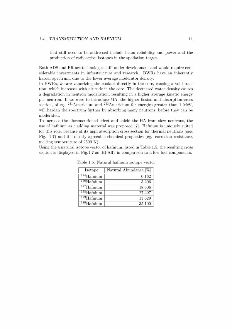
Both ADS and FR are technologies still under development and would require con-siderable investments in infrastructure and research. BWRs have an inherentlyharder spectrum, due to the lower average moderator density.In BWRs, we are vaporizing the coolant directly in the core, causing a void frac-tion, which increases with altitude in the core. The decreased water density causesa degradation in neutron moderation, resulting in a higher average kinetic energyper neutron. If we were to introduce MA, the higher fission and absorption crosssection, of eg. 241Americium and 243Americium for energies greater than 1 MeV,will harden the spectrum further by absorbing many neutrons, before they can bemoderated.To increase the aforementioned effect and shield the HA from slow neutrons, theuse of hafnium as cladding material was proposed [7]. Hafnium is uniquely suitedfor this role, because of its high absorption cross section for thermal neutrons (see:Fig. 1.7) and it’s mostly agreeable chemical properties (eg. corrosion resistance,melting temperature of 2500 K).Using the a natural isotope vector of hafnium, listed in Table 1.5, the resulting crosssection is displayed in Fig.1.7 as ’Hf-All’, in comparison to a few fuel components.
Table 1.5: Natural hafnium isotope vector
Isotope Natural Abundance [%]174Hafnium 0.162176Hafnium 5.206177Hafnium 18.606178Hafnium 27.297179Hafnium 13.629180Hafnium 35.100

12 CHAPTER 1. MOTIVATION
Figure 1.7: Compare cross sections of TRU-elements with natural hafnium
The fission cross sections of all transuranic elements, present in the initial isotopevector (see: Table 4.1), are greater by a factor of 10 to 100 then the absorptioncross section of natural hafnium for incident energies of 1 MeV and greater (see:Figure 1.7 for a selection of TRU-elements). Parity is usually reached in the areaof 0.5 to 0.1 MeV, only 239Plutonium, 241Plutonium and 245Curium prove to beexceptions to this rule by maintaining a fission cross section equal or greater thanthe hafnium. The overall burn-up of these elements is likely to be unaffected though,as they have all both considerable cross section and fission propability in the higherneutron energy ranges. Decisive for the effectiveness of hafnium are the resonancepeaks between 1 and 10 eV, which have cross sections between one and two ordersof magnitude greater than anything else in this energy range, depleting the thermalspectrum below them.

Chapter 2
Theoretical Background
In this chapter we want to give a short overview over the must important equations,employed in our simulations, as the computer codes are founded on an understand-ing of, and made to solve, them. A mathematically correct, step-by-step derivationwould go beyond the scope of this work and is available in any number of reactorphysics text books, therefore we will content ourselves with an outline:
1. Bateman Equation
The Bateman Equations is a set of coupled, linear, first order, inhomogenousdifferential equations, describing abundances and activities of elements in amaterial, subjected to a neutron flux φ, as a function of time.
dNi
dt= −
∑j 6=i
[λdji +
∫φ(E, t)σtrjidE
]Ni︸ ︷︷ ︸
Depletion
+∑j 6=i
[λdij +
∫φ(E, t)σtrijdE
]Nj︸ ︷︷ ︸
Production
(2.1)where Ni is the concentration of isotope i in the material, φ(E, t) the neutronflux of Energy E, λdji the decay constant and σtrji the total transmutation crosssection from isotope i to j, including all reactions with the exception of elasticscattering and inelastic two-body scattering [9].In Serpent, it is used to track fuel depletion and burn-up in single assemblyor fuel type. The equations for different isotope concentrations are coupledby depletion and production terms. In matrix form the problem is:
−→n = A−→n (2.2)
where −→n is the vector containing the isotope concentrations of all relevantnuclides and A the attendant matrix of coefficients. This can be solved bythe matrix exponential method, yielding the solution:
−→n (t) = eA(t−t0)−→n (t0) (2.3)
13

14 CHAPTER 2. THEORETICAL BACKGROUND
where n(t0) is the initial isotope vector. The exponential of the matrix Acan be solved with various numerical methods. Serpent currently employs theTransmutation Trajectory Analysis Method (TTA) or the Chebyshev Ratio-nal Approximation Method (CRAM) [10].
2. Neutron Transport Equation
The Neutron Transport Equation, at its core, is rather simple. It has rootsin the Boltzmann Equation and states the conservation of the total neutronand delayed neutron number in a volume element of phase-space. To put itanother way, assuming the source term to be 0 in a given energy/space in-terval, any change in neutron number will be equal to the sum of in and outscattering neutrons.
∆Neutrons = Production− Losses (2.4)
The actual equation is slightly more involved. Setting up the particle densitybalance inside an infinitesimal volume element d3r = dx · dy · dz at position−→r , with a differential solid angle d−→Ω around the direction of motion −→Ω anda energy interval dE around E, gives us [9]:
1v
∂
∂tψ(−→r ,−→Ω , E, t)+−→Ω ·∇ψ(−→r ,−→Ω , E, t)+Σt(−→r , E)ψ(−→r ,−→Ω , E, t) = q(−→r ,−→Ω , E, t)
(2.5)where ψ is the angular neutron density and Σt the macroscopic total crosssection of the medium. Moving from left to right, the equation consist of thetime-wise change in neutron density, the change in neutron flux with positionvector and all scattering or absorption interations, removing neutrons fromthe flux, and finally a general source term q(−→r ,−→Ω , E, t), which can be splitin three parts:
q = q(−→r ,−→Ω , E, t)ex︸ ︷︷ ︸external
+ q(−→r ,−→Ω , E, t)s︸ ︷︷ ︸scattering
+ q(−→r , E, t)f︸ ︷︷ ︸fission
(2.6)
q(−→r ,−→Ω , E, t)ex =∫
4π
∫ ∞0
Σs(−→r ,−→Ω ′ → −→Ω , E′ → E) d−→Ω ′dE′ (2.7)
q(−→r , E, t)f = 14π
∫ ∞0χ(E)νΣf (−→r , E′)ψ(−→r , E′, t)dE′ (2.8)
where qex returns the rate at which neutrons are emitted by external sources,qex gives us the neutrons scattered into the current phase-space element (−→Ω , E)from all other Energies and differential solid angles (,−→Ω ′, E′). If more thanone isotope is present in the scattering medium, Σs has to be replaced by theweighted sum over all macroscopic cross sections. qf is the source term for

15
neutrons produced in fission events with χ(E) as the fission spectrum, mean-ing the probability for a neutron to be emitted in a given energy interval, andthe neutron production term νΣf (−→r , E′), consisting of the average number ofemitted neutrons ν and the macroscopic fission cross section Σf .The neutron transport equation, as quoted above, is correct, but not the mostadvantegous to describe neutron behaviour in a reactor. Integration of d−→Ωover 4π of the unit circle will remove the dependency on the solid angle. Wealso replace the second term in Equation (2.6), describing the change of theneutron density with the spatial derivative, with the angular current density−→j (−→r ,−→Ω , E), the integration of the equation over the full space-angle willyield the neutron current density −→J (−→r , E).
3. Group Diffusion Equation
Using Fick’s Law:−→J g(−→r , t) = −Dg(−→r )∇Φg(−→r , t) (2.9)
withΦg(−→r , t) =
∫V
∫ Eg−1
Egψ(−→r ,−→Ω , E, t)d−→r d−→Ω dE (2.10)
where −→J g(−→r , t) is the neutron current density, Dg(−→r ) the diffusion coefficient,Φg(−→r , t) the scalar, spectrum averaged neutron flux and g the energy groupindex. With this we can set up the group diffusion equation:
1v
∂
∂tΦg(−→r , t)−∇Dg(−→r ) · ∇Φg(−→r , t) + Σt,gΦg(−→r , t) =
G∑g′=1
[Σs,g′→g(−→r )Φg′(−→r , t)
]+ χ
G∑g=1
[νΣf,g(−→r )Φg(−→r , t)](2.11)
where g is the energy group index, Σt,g the transport cross section, Σs,g′→g thescattering cross section from energy group g to g’ and Σf,g′ the fission crosssection. Altogether we get a set of coupled differential equations, one equationper energy group per material, connected by boundary conditions and thedemand of continuity. An often employed approximation is the two groupmethod, dividing the energy spectrum in two intervals (g=2), fast neutronsfor energies greater than 0.625 eV and thermal neurons below that. Dependingon the accuracy of the model and the nuclear data libraries involved in thesimulation six to eight energy groups are also often used.If the geometry is sufficiently complicated, as in, for example, a BWR, wehave to make certain simplifications. We cut necessary computing power byreducing the resolution of the model, replacing the three-dimensional spatialcoordinates with by homogenized divisions with constant cross sections, known

16 CHAPTER 2. THEORETICAL BACKGROUND
as nodes. Neighboring nodes are still coupled by boundary conditions andcontinuity. The final, discretized form is:
1vng
∂
∂tΦng −
(−→J n+g −
−→J n−g
)+ Σn
t,gΦng =
G∑g′=1
[Σns,g′→gΦn
g′
]+ χ
G∑g=1
[νp,gΣn
f,gΦng
](2.12)
where n is the index of the node, Φng the node average flux and −→J n±
g thesurface average net current, where the superscript plus and minus representthe positve and negative surface sides of the node. For a full calculation,equation (2.12) should also include the precursor Cng density:
1vng
∂
∂tΦng −
(−→J n+g −
−→J n−g
)+ Σn
t,gΦng =
G∑g′=1
[Σns,g′→gΦn
g′
]+ χd,k
K∑k=1
λkCnk + χp,g
G∑g=1
[νp,gΣn
f,gΦng
] (2.13)
and∂
∂tCnk = 1
keff
G∑g=1
[νd,g,kΣn
f,gΦng − λkCnk
](2.14)
where p and d notify prompt and delayed neutrons, respectively and λk is thedecay constant of the k-te precursor group.
4. Short Outline of Basic Neutronic Problems
The steady-state is time independent and defined by the balance of neutronproduction through fission and scattering on the one side and neutron loss byleakage and absorption on tht other. We drop the time derivative and get:
n∑t,g
Φng −
(−→J n+g −
−→J n−g
)=
G∑g′=1
[Σns,g′→gΦn
g′
]+ 1keff
χs
G∑g=1
[νΣn
f,gΦng
](2.15)
Transforming the set of equations above into matrix form, where F containsall fission terms and M all migration terms, we get:
MΦ = 1keff
FΦ (2.16)
The eigenvalue keff is necessary to compute the time-wise change in the neu-tron flux and hence burn-up and power output. Furthermore all transientcalculations in TRACE/Pracs require an initial steady-state calculation to

17
initialize the core conditions. The problem is solved in PARCS by a combi-nation of fission source iteration method, see equation (2.17), and Wielandteigenvalue shift method [11], see equation (2.18):
MΦt+1 = 1kteff
FΦt (2.17)
(M − 1
ktsF
)Φt+1 =
(1kteff− 1kts
)FΦt (2.18)
where t is the index of the time-step and the Wiedland shift is obtained bysubtracting a fission source from both sides kts = ktA + δk. Equation (2.18)can be rewritten as:
knAΨt+1 = FA−1Ψt+1 (2.19)
using the following definitions:
1ktA≡(
1kteff− 1kts
), Ψ ≡ FΦt, A ≡
(M − 1
ktsF
)(2.20)
The eigenvalue kA is updated by:
kt+1A = ktA
〈Ψt+1 | Ψt+1〉〈Ψt+1 | Ψt〉
(2.21)
The iteration can be repeated until the eigenvalue has converged.
5. Assembly Discontinuity Factor
The nodal form of the diffusion equation, see page 16, can be solved analyti-cally with local flux solutions, coupled to each other by sets of boundary condi-tions. Regrettably the so achieved flux shapes are often not very accurate. Wecan solve this problem by allowing discontinuities at node boundaries, thatallow more accurate volume-integrated reaction rates and surface-averagedcurrents/fluxes. These are known as assembly discontinuity factors and aredefined as the ratio of surface-integrated to volume-integrated flux:
ADF =
1A
∫A
∫ Eg−1
Egψ(−→r , E)d2−→r dE
1V
∫V
∫ Eg−1
Egψ(−→r , E)d3−→r dE
(2.22)


Chapter 3
Methodology
3.1 Objective
The central point of this work, is to find a configuration, that combines a netHA burn-up with a power distribution sufficiently stable to be able to perform ina design-expected accident scenario and study the performance, depending on theHA-content . To this end we will build on the results of Wallenius & Westlin [7] andSuvdantstseg [12], adapt them to the situation at hand and find our own solution,optimized for burn-up within the framework of relevant safety regulations.To be able to introduce new fuel configurations (isotope vectors, geometry, boundaryconditions) into the accident simulation, we will develope software, that bridgesthe gap between the monte carlo burn-up code Serpent and the TRACE/PARCScoupled code, used to simulate the accident scenario.
3.2 Outline of Method
The aim of this study was to determine the optimal configuration for HA burn-upin BWR with hafnium cladding and to study the effects the new cladding and fuelloading has on the behaviour of the BWR in an accident scenario. To this end wewill have to employ several interlocking pieces of simulation software.The monte carlo simulation code Serpent will be used to determine the burn-upand macroscopic cross sections of different spatial fuel configurations, using theENDF/B-VIII libraries for nuclear data. The PARCS software employs numeri-cal methods like the theta and the Wielandt eigenvalue shift method to solve thetime-dependent behavior of the spatial neutron flux equation. PARCS is coupledto TRACE, a general thermal-hydraulic computational system, which models thebehaviour of the coolant/moderator in the accident scenario, while PARCS is re-sponsible for the computation of the power output. To this end, PARCS relies onan input file, containing the relevant macroscopic cross section data, specific to onefuel configuration, details see page 41. The only way to introduce a new configura-tion, is to introduce a new file.
19

20 CHAPTER 3. METHODOLOGY
Once a configuration is selected, cross section data has to be produced seperatelyfor each fuel layer. This data has to be translated in a input format, which willbe accepted by PARCS, by a dedicated matlab script. The PARCS input-file, fromhere on refered to as PMAX, has to meet certain requirements, to produce a reli-able output. The exact scope necessary, depends on the system to be modelled andthe accident scenario, in our case we have to provide for every fuel type and everyburn-up step:
• six cross sections for varying moderator densities,
• six cross sections for varying moderator densities with inserted CR and
• six cross sections for varying moderator densities with a different fuel temper-ature.
Serpent is not able to take into account parameter changes during a burn-up run.Therefore, if we want a fuel with 15 burn-up steps and the above configuration of 18data points, we will need to run one serpent burn-up calculation with 15 burn-upsteps and 18 simulations at each time-step, building on the momentary fuel vectorsproduced in the burn-up calculation, totalling at 271 simulations per fuel type.To reiterate, we need the following steps to produce a viable PMAX input-file:
• simulate the full assembly in Serpent, with x different fuel types, to determinethe optimal fuel loading.
• For all x fuels, run a burn-up calculation in Serpent with y steps.
• For all y burn-up steps and x fuels, run a simple steady-state Serpent simu-lation, moving through a list of z possible values for our boundary conditionslike, eg. CR position, moderator density, fuel temperature, boron content ofmoderator etc. Input fuel vectors have to be identical to the ouput of theburn-up calculation for the the appropriate burn-up step.
• Altogether we get x times y times z plus 1 simulations to run.
The output files of these simulations will then be scanned and read out into thePMAX-file format, that can be feed into the TRACE/PARCS coupled codes. Ob-viously, the higher the desired accuracy in the TRACE/PARCS simulation, thehigher the number of data points, and therefore the number of Serpent simulations,necessary for the PMAX-file production.The TRACE simulation itself, in the configuration chosen by us, consist of threesteps:
1. Establishing a stable baseline for the required geometry; power output is setto a constant value in this step and the coupling with PARCS is deactivated.

3.3. VERIFICATION OF METHOD 21
2. Using the output of the first simulation as a restart point, we start the steadystate evaluation. The power is now controlled by the neutron flux, whichis computed in PARCS with the help of the previously constructed PMAX-files, but still fixed to a value given by the user. The steady state outputwill contain normalized power distributions. If these do not fulfill stabilitycriteria, the user is recommended to modify the fuel distribution and rerunthe steady state, until they do.
3. Again, using the output of the steady state evaluation as the restart file westart the actual transient calculation. PARCS is activated and the power levelis free-floating. It is considered good practice to leave the simulation undis-turbed for a certain amount of time before triggering the accident scenario,to validate the steady state solution in use.
3.3 Verification of MethodTo show the validity of the method, outlined on page 19 et seq., we produce aPMAX-file for generic UOX-fuel with an 3.7 % enrichment in 235U and compareit to the original cross sections for the Ringhals-1 reactor, abbreviated as ’OrgXS’in the plots below. The original consist of 25 different PMAX files, arranged in acomplex radial and axial pattern.Regretably, the isotope vectors, corresponding to the fuels used to produce thiscross-sections, are unknown to the author. Repeated attempts to determine thecompositon proved to be unsuccessful. Therefore we elected to use a fuel based onthe standard Westinghouse BWR-fuel with an even axial and radial distribution,henceforth refered to as Config.0. The keff -value, as computed by PARCS, givesus 0.975 for the steady state computation of the original cross-sections and 1.045for Config.0, indicating a lower average fissile material content in the original cross-sections. We compare the behaviour of a few important parameters for reactorsafety, for a turbine trip followed by a SCRAM or a screw-in of the CR. For adetailed describtion of the accident scenario see page 51.Unsurprisingly the, presumed, higher fissile content results in a higher power spike,at the beginning, and a more drawn out power curve, during the shutdown, indi-cating a more bottom-heavy fuel distribution in the original.

22 CHAPTER 3. METHODOLOGY
0 50 100 150 200 250 300
Time (s)
0
5e+08
1e+09
1.5e+09
2e+09
Pow
er (
W)
OrgXS
Config_0
Figure 3.1: Power output of OrgXS and Config. 0 during SCRAM
25 26 27 28 29 30
Time (s)
0
5e+08
1e+09
1.5e+09
2e+09
Pow
er (
W)
OrgXS
Config_0
Figure 3.2: Zoom: Power output of OrgXS and Config. 0 during SCRAM

3.3. VERIFICATION OF METHOD 23
0 50 100 150 200 250 300
Time (s)
7e+06
7.2e+06
7.4e+06
7.6e+06
7.8e+06
Pre
ssur
e (P
a)
OrgXS
Config_0
Figure 3.3: Steamdome pressure of OrgXS and Config. 0 during SCRAM
Higher power output results in a faster rise of the steam dome pressure, resulting inthe activation of the ADS overpressure-valve, recognizable due to the characteristicpressure spike at 28 seconds.
0 50 100 150 200 250 300
Time (s)
5
6
7
8
9
Le
ng
th (
m)
OrgXS
Config_0
Figure 3.4: Waterlevel of OrgXS and Config. 0 in reactor vessel during SCRAM

24 CHAPTER 3. METHODOLOGY
Correspondingly, the simulation, for the CR screw-in, gives us higher power spikesfor Config. 0, resulting in faster growing pressure and a greater discharge throughthe ADS-valve, which in turn gives us a lower waterlevel in the core.
0 100 200 300 400 500
Time (s)
0
1e+09
2e+09
3e+09
4e+09
Pow
er (
W)
OrgXS_2
Config_0
Figure 3.5: Power output of OrgXS and Config. 0 during screw-in
0 100 200 300 400
Time (s)
7e+06
7.2e+06
7.4e+06
7.6e+06
7.8e+06
8e+06
8.2e+06
Pre
ssur
e (P
a)
OrgXS
Config_0
Figure 3.6: Steamdome pressure of OrgXS and Config. 0 during screw-in

3.4. ALGORYTHM TO PRODUCE A VIABLE TRANSIENT SIMULATION 25
0 100 200 300 400 500
Time (s)
4
5
6
7
8
9L
en
gth
(m
)
OrgXS
Config_0
Figure 3.7: Waterlevel of OrgXS and Config. 0 in reactor vessel during screw-in
Summing up, we have shown the feasiblity of a simulation with a PMAX-file, pro-duced for an UOX-fuel and the results are, while not exactly validated, at leastshown to be plausible within the boundaries of our capabilities.We could establish a fuel with a keff -value, and presumably a fissile content, closerto the original, but as the isotope composition used to produce the original fuelcross sections is still unknown and we therefore lack a benchmark with which wecould compare our creation, this approach seems to hold little additional value.A possible solution might be to submit an isotope vector to CASMO-4, the industrialcode used to produce PMAX-files and compare the results of a simulation run witha self-produced PMAX-file with the results of an industry produced PMAX-file.
3.4 Algorythm to produce a viable Transientsimulation
1. Produce a satisfactory burn-up for a full, z-dependent fuel distribution
2. FOR ALL distinct fuel types from 1, perform a burn-up calculation
3. FOR ALL burn-up steps, boundary conditions and distinct fuel types from1, perform a Serpent steady state computation. Details on page 19.
4. Translate the output into PMAX-files, as discussed in detail on page 41 etseqq.

26 CHAPTER 3. METHODOLOGY
5. Produce a TRACE-model for the system, we want to simulate, use it’s outputas a restart file for the TRACE steady state computation. Details, see page20.
6. IF the axial and radial power distributions of a TRACE/PARCS steady statesimulation with the given fuel geometry and TRACE-input are satisfactory,continue ELSE Modify the fuel distribution to be more stable and reiteratefrom 1.
7. IF the transient simulation fullfills safety conditions (max. pressure, temper-ature, etc.) we are done ELSE Modify TRACE-input and reiterate from 5.or modify fuel distribution and reiterate form 1.

Chapter 4
Serpent Modelling
The model for our simulation is Ringhals-1. The assemblies measure 13.90 cm onthe side, filled with a rectangular water rod, measuring 3.5 by 3.5 cm, and 91 fuelpins, with an outer radius of 0.551 cm, a fuel radius of 0.49 cm and a pin pitchof 1.295, containing five different kinds of fuel, with varying TRU-enrichment. Weemploye 48 fuel pins with four times the baseline enrichment, 14 fuel pins with threetimes the baseline, 16 with two-and-a-half times the baseline, 9 with one-and-a-halftimes the baseline and 4 with baseline enrichment. The fuel pins are distribution isdesigned to minimize power peaking at the assembly edges.The cladding of the fuel rods, the assembly and the waterchannel and consists ofzircaloy with a variable hafnium content, which is set to 5.00% unless otherwisementioned.A horizontal cut through an example assembly is displayed in Figure 4.1.Vertically the fuel assembly extends for 370.45 cm and is subdivided in 25 fuel zones.The simulation employs reflective boundary conditions in x and y-direction, makingit functionally infinite, and black boundary conditions in z-direcition.The cruciform control rod extends for 10.06 cm from it’s point of origin into thewater gap. The arms of the cross, only half visible in the figure below, have athickness of 1.08 cm. The CR, although visible in Figure 4.1, will not be presentin any of the full assembly simulations. CR are only extended to produce crosssections for single fuel type simulations with a fitting set of boundary conditions.
27

28 CHAPTER 4. SERPENT MODELLING
Figure 4.1: Cut through the x-y-plane of a fuel assembly
To model a BWR correctly, we have to take into account the void fraction variationover the length of the z-axis of the reactor. For the burn-up calculation treadingthe coolant flow as stacked layers of decreasing, temporal constant density is suf-ficient as a simplification. The full thermohydraulic model will be applied in theTRACE/PARCS simulation. To maintain comparability between the original fuelloading of Ringhals-1 and the hafnium fuel, we will adopt the density data pointspreset by the original PMAX-files. The reference point for coolant density in theoriginal PMAX-file is 0.45858 g/cm3. We adjust the known void profile of a BWR(see: Figure 4.2) to return this density value as the arithmetical mean and employthe result in our core Serpent simulation. To convert void fraction to density, weuse:
ρ = (1− α)ρliq + αρvap (4.1)where α is the void fraction, ρliq = 0.73992 g/cm3 the water density [8] and ρvap =0.03652 g/cm3 the steam density [8], both at 70 bar pressure. To reiterate, thedensity distribution displayed in Figure 4.2 will only be used to compute the burn-upfor different fuel compositions and spatial distributions. Cross sections for PMAX-files are produced for a single fuel layer with a constant coolant density.

4.1. FUEL VECTOR 29
Figure 4.2: Coolant density distributions
4.1 Fuel Vector
Two kinds of fuel are in use in this simulation, standard UOX-fuel, enriched to1.35 %, and MOX-fuel, produced from 4.2 % enriched UOX, after a burn-up of 50MWd/kgHM and a cooling time of 4 years [3]. The element ratio of Pu/Am/Cmis 93.6/5.6/0.8 for normal MOX fuel. To achieve a net burn-up the baseline HA-content was increased to 87.5/10.9375/1.5625. The isotope vectors are displayedin detail in Table 4.1. The fuel is set to a power density of 25 W/g of heavy metal.
Isotope Fraction [%] Isotope Fraction [%] Isotope Fraction [%]238Pu 3.5 241Am 58.1 244Cm 91.9239Pu 51.9 242Am 0.2 245Cm 6.6240Pu 23.8 243Am 41.7 246Cm 1.5241Pu 12.9242Pu 7.9
Table 4.1: Isotope fractions of fuel vector as atomic density
The ratio of TRU elements will remain constant, unless otherwise mentioned, butthe TRU-content of the fuel as a whole will be the main variable through the Serpentpart of this discussion.

30 CHAPTER 4. SERPENT MODELLING
4.2 Investigated Fuel DistributionsTo find the optimal spatial configuration for burn-up, we vary the axial distributionof the TRU-enriched fuel elements, the TRU-content itself, the HA-fraction of theTRU and the Hf-fraction of the cladding. The results are summarized in Table 8.1.There are two fuel configurations, we want to consider in detail:
Configuration 1:
Config. 2 is optimized for maximal burn-up of HA. We replace the UO2 withMOX-fuel of two different TRU-concentrations; 19 layers with 14.20% of TRU and6 enriched layers, located at the top of the fuel pin, where we will find the low-est moderator density and therefore the hardest neutron spectrum, with 23.68%of TRU, yielding an overall TRU-content of 16.48%. The hafnium content of thecladding will be a constant 5% over the whole length of the assembly.
Figure 4.3: Configuration 1: MOX-fuel pin with TRU-enriched layer in fourth quar-ter; top: 23.68% TRU, bottom: 14.21% TRU; 16.48% TRU altogether
Configuration 2:
Alternative vertical fuel distribution, designed to yield optimal stability and ful-fill safety regulation demands for the normalized vertical powershape. The trade-offis a reduction in maximal possible burn-up of fuel in general and HA in particular.
Figure 4.4: Configuration 2: MOX-fuel pin with 4 layers of TRU-enrichment; fromtop to bottom: 14.00% TRU, 16.00% TRU, 19.00% TRU, 20.00% TRU; 16.48%TRU altogether

Chapter 5
Selection of viable fuelconfigurations
To find the optimal configuration for burn-up we vary the spatial distribution of theTRU-enriched fuel elements, the TRU-content itself, the HA-fraction of the TRUand the Hf-fraction of the cladding.Our objective is to find a constellation that will contain enough HA and a hardenough neutron spectrum to yield an acceptable burn-up, while still being reliantenough on thermal neutrons to be controlable during a transient and fulfilling safetystandards for our axial and radial power distributions.
5.1 Burn-up results
A detailed list of all considered configurations would go beyond the scope of thiswork, but a short summary of all burn-up results is presented in Table 8.1, normal-ized by ton of fuel and energy produced in TWhth.
Table 5.1: HA & Pu burn-up for varying axial fuel distributions 2
Burn-Up Config. 1 Config. 2in MWd/kgHM
∑HA
∑Pu
∑HA
∑Pu
0 1.00000 1.00000 1.00000 1.000005 1.01111 0.97923 1.01216 0.9797610 1.01358 0.96277 1.01482 0.9617615 1.01178 0.94399 1.01286 0.9449820 1.00753 0.92776 1.00861 0.9292030 0.99461 0.89737 0.99670 0.8988740 0.97960 0.86862 0.98264 0.8702750 0.96364 0.84123 0.96737 0.84262
31

32 CHAPTER 5. SELECTION OF VIABLE FUEL CONFIGURATIONS
It is unsurprising that configurations, which concentrate the TRU-elements in theregion with the lowest moderator density and therefore the hardest neutron flux,will achieve the best burn-up results.For the purpose of maximising the destruction of HA, Config. 1 is optimal. Furtherimprovements are most easily made by shifting more of the TRU-elements upwardsalong the z-axis and by increasing the percentage of HA-elements in TRU.It should be noted though that increasing hafnium contents of the cladding over 5%seems to make the burn-up performance worse, see Table 8.1, owing probably to aseverly decreased neutron-flux.
5.2 Power DistributionA major limiting factor for the various geometries are regulations for the radial andaxial power peaking factors, therefore we use the output of the TRACE/PARCSsteady state simulations to display the relevant power distributions.The ideal power distribution is cosinus-shaped, while triangle-shaped distributionsare regarded less favourable and two peaked distributions even less so, as the inertiaof a smaller side maximum, and therefore it’s resistance to an oscillation, is easierto overcome by an outside excitation. For a radial distribution several power peaksare acceptable if the distribution is symmetric.The general accepted limit for the volumetric normalized power peaking factor is2.5, 1.5 is a recommended maximal value for both axial and radial power peaking,although, as demonstrated in the plot ’Original XS’, representing the cross sectionsof the original UO2-fuel loading of the Ringhals Reactor, recommendations are notalways strictly followed.The maximum for ’Configuration 2’ is found at 1.52 and2.101 for ’Configuration 2a’. Configuration 1’ proved to be unable to produce aviable steady state.At this point, we should note though, that the simulation was run with a full coreloading of fresh fuel, which will occure only once during the life time of a reactor.Higher burn-up in the better moderated lower regions will degrade the peak overtime. Refueling is usually done in increments of approximately 20% at a time,therefore the power distribution displayed in Figure 5.1 is an extreme, which shouldnot be reached again, assuming normal operating patterns.

5.2. POWER DISTRIBUTION 33
Figure 5.1: Axial, normalized power distribution of various fuel distributions
Cut through the diameter of the normalized radial power distribution. Note thejag-like form of the power-distribution, caused by partly inserted CR.
Figure 5.2: Radial, normalized power distribution of various fuel distributions

34 CHAPTER 5. SELECTION OF VIABLE FUEL CONFIGURATIONS
’Configuration 1’ , as already mentioned, could not complete it’s simulation and wasreplaced with ’Config. 1a’, which uses only 19.00 % enriched TRU in it’s topmostfuel layers but is otherwise identical to ’Config. 1’, to at least give us an idea, aboutthe safety performance of the ideal HA-burner. Concentrating the majority of theTRU-fuel in the topmost parts of the assemblies, where the moderator density islowest and the neutron spectrum hardest, allows it to use it’s ability to fission fromfast neutrons to full effect. Consequently the normalized power distribution heavilyshifted to the top, with virtually no power output in the lower third of the reactor.Even in the reduced constellation, the power peak is with 2.705 the tallest of allconsidered configurations. The volumetric power limit is exceeded, before we evenconsider the radial power distribution. It is highly probable that all undesirabletraits would just become more extreme, if the original enrichment was restored.Therefore ’Config.1’ was discarded.’Configuration 2’ was produced as a compromise solution by gradually shifting TRU-content downward, iterating through several possible configurations (not displayed),until a satisfactory results was achieved. The 19.00% TRU-enriched fuel layer wasintroduced to provide a gradual change between the 20.00% enriched bottom and the16.00% enriched centerpiece, because large, abrupt changes in TRU-concentrationmay result in local power peaking and abrupt neutron flux changes at the interfaceregion. Note that this local maxima may be to small to show up in the averageddistribution, plotted in Figure 5.1. The topmost, 14.00% enriched layer was intro-duced to counteract a small power peak at the top.Altogether ’Configuration 2’ makes for an acceptable fuel distribution, combininga noticeable burn-up, a fairly even, axial power distribution and, in the 12.50 %HA-edition at least, the smallest bottom power peak. This may indicate that theincreased moderation in the lower parts of the core has a lesser effect on the MOX-fuel, although this explanation seems to clash with the behavior of ’Config.2’ withincreased HA-content. We may also notice the smaller indents at the CR-positionsfor ’Config.2’ and ’Config.2a’, indicating the smaller relative weight of the bottomlayers, where the partly inserted CR make their influence felt.
There is a noticeable correlation between the quality of the power distribution andthe ability of the simulation to complete. As a typical TRACE/PARCS simulation,running for 400 seconds of in-simulation time, can take, depending on availablehardware and examined transient, anything between 2 and 4 days to complete, avetting process using the steady state results is strongly recommended to avoidtime-consuming dead ends.Generally we can say that the higher TRU-content of a fuel configuration the moreoften they tend to crash. Keeping all other factors constant but the fuel distribution,we can see, that the average TRU-content is not the only variable of importance,spatial distribution and relative enrichment of different fuels also contribute. Notethat ’Config.1’ and ’Config.2’ have the same averaged isotope and cladding vector,but only ’Config.2’ was able to produce a steady state result. A possible contribut-ing factor to this phenomenon might be local power peaking and abrupt neutron flux

5.2. POWER DISTRIBUTION 35
changes at the interface between to regions of strongly varying TRU-enrichment,particularly if one of them contains standard fuel. Also, the fuel vector employedin this simulations is balancing precariously on the edge of a positive void worth,’Config. 1’ may have failed because of the concentration of TRU-elements in theupper quarter and the resulting increase in relative weight of fast fission reactions.


Chapter 6
TRACE/PARCS software suite
6.1 TRACE"The TRAC/RELAP Advanced Computational Engine (TRACE - formerly calledTRAC-M) is the latest in a series of advanced, best-estimate reactor systems codesdeveloped by the U.S. Nuclear Regulatory Commission for analyzing transient andsteady-state neutronic-thermal-hydraulic behavior in light water reactors." (see ref-erence [14])TRACE has been designed to perform best-estimate analyses of loss-of-coolant acci-dents, operational transients, and other accident scenarios in PWRs and BWRs. Itis capable of simulating an entire primary system with pipes, pumps, turbine, steamdryers, reactor vessel and more. Each piece of physical equipment is representedby a simulation component, which in turn is further broken down into a number ofuser-defined cells, over which fluid, conduction and kinetics equations are averged.TRACE is equipped to solve multidimensional two-phase flows, general heat trans-fer and core-wide point kinetics equations without spatial resolution. If a moredetailed modelling of the neutron kinetics is needed, TRACE can be coupled to asuitable code, in our case PARCS.
6.1.1 TRACE Model
The central piece of the trace model is the reactor vessel, the active core consistingof 325 CHAN-stuctures, each one coupled to PARCS to determine it’s power outputand reactivity feedback. The CHAN-stuctures are arrayed in a half-core symmetricmodel to simulate 650 fuel assemblies, see Figure 6.2. Also contained in reactorvessel are the steam seperators, steam dome and downcomers.Connected to the vessel are 6 PIPE-structures, the steamline, the feedwater line,the bypass line, the outgoing and incoming connection to the recirculation pumpand the connection to the ADS safety relieve valve.The outgoing connection links the recirculation pump with the lowest level of thedowncomer, while the incoming connection loops back to the lower plenum.The ADS valve is connected to the reactor vessel just above the steam seperators
37

38 CHAPTER 6. TRACE/PARCS SOFTWARE SUITE
Figure 6.1: TRACE Model
Figure 6.2: TRACE Core Map

6.2. PARCS 39
and dryers and intended to relief overpressure and the resulting stress on the reactorvessel, by releasing steam to the containment. It consists of three banks of valves,which are triggered with rising pressure, at 7.90, 8.02 and 8.20 MPa, respectively.The FILL- and BREAK-compenent, connected to the steamline and feedwater line,respectively, impose pressure and mass-flow boundary conditions. Essentially theFILL-component provides a coolant flow from an unlimited reservoir, while theBREAK-component absorbs it into an equally unlimited reservoir. The outflowfrom the system into the BREAK is tied as a feedback loop into the control-logicof the inflow from Fill-component.
6.2 PARCS
The Purdue Advanced Reactor Core Simulator (PARCS) has been designed to cal-culate spatial kinetics problems. To this end PARCS needs to solve the eigenvalueproblem and the time-dependent neutron transport equations. "The first step inthe solution of either process is to discretize the balance equations in both timeand space. For the temporal discretization, the theta-method with exponentialtransformation is employed in PARCS along with a second-order analytic precur-sor integration technique. The temporal discretization scheme allows sufficientlylarge time step sizes even in severe transients involving super-prompt critical re-activity insertion. For spatial discretization, the efficient nonlinear nodal methodis employed in which the coarse mesh finite difference (CMFD) problems and thelocal two-node problems are repetitively solved during the course of the nonlineariteration." (see reference [13])
6.2.1 PARCS Model
The PARCS Model consists of axial 27 layers, each layer corresponding to a node,25 of which are fuel containing, while the top and bottom most are representingreflectors. We differentiate top-, bottom- and radial-reflectors, each type with it’sown cross sections. Radially we have 650 fuel assemblies, each corresponding to anode, surrounded by another layer of reflectors, see Figure 6.3.In the displayed example, see Figure 6.3, ’26’ signifies a radial reflector assembly,everything else (’3’ ,’5’ ,’6’ ,’8’ ,’11’ ,’14’ ,’16’ ,’24’) are different types of fuel orassembly geometry. The number of fuels will obviously depend on the choices of theauthor and the desired level of detail. The example was taken from the geometryfile of the original cross section. Self-produced models, in this work, usually havenot more than four different fuel types.The PARCS Model also contains 15 CR-banks with altogether 157 CR, 42 of whichare totally or partly inserted during normal operations.

40 CHAPTER 6. TRACE/PARCS SOFTWARE SUITE
Figure 6.3: PARCS Core Map
6.3 TRACE/PARCS coupling
"The reason for using coupled thermohydraulic/neutron kinetic (TH/NK) is that anuclear power plant is a strongly coupled system of thermal-hydraulics and neutronkinetics. The space- and time-dependence of the neutron flux in the reactor coreis dependent on the cross-sections and kinetic parameters. The cross-sections andkinetics parameters are themselves dependent on the fuel and coolant temperature.An accurate prediction of the thermal-hydraulic conditions in the reactor is thus aprerequisite for an accurate prediction of the neutron flux. The neutron flux in turninfluences the heat released by the fission and therefore the distribution of the fueland coolant temperature. Only coupled TH/NK codes are able to solve this kindof problem." (see reference [18])The coupling of TRACE/PARCS is achieved through a simple code-to-code dataexchange. Thermal-hydraulic parameters generated by TRACE (moderator tem-perature, liquid density, vapour density, void fraction, boron concentration, fuel av-erage temperature, fuel centreline temperature, fuel surface temperature) are sent toPARCS, neutronic parameters generated by PARCS (total power, power depositedin the moderator through direct moderator heating, power deposited in the fuel)

6.4. PARCS AND THE PMAX-FILE FORMAT 41
are sent to TRACE. The data exchange is illustrated in Figure 6.4. There is one
Figure 6.4: Schematic of the TRACE/PARCS data exchange, [18]
data exchange per time step and the coupling is first-order in time and explicit.The calculation logic within one time step iteration is as follows:
1. TRACE receives nodal power from PARCS.
2. TRACE calculates new thermal-hydraulic solution for coolant and fuel basedon nodal power received from PARCS.
3. TRACE sends its thermal-hydraulic solution to PARCS.
4. PARCS receives thermal-hydraulic solution from TRACE.
5. PARCS updates macroscopic cross-sections based on thermal-hydraulic solu-tion received from TRACE.
6. PARCS solves 3D neutron diffusion equation and calculates nodal power.
7. PARCS sends nodal power to TRACE.
6.4 PARCS and the PMAX-file format
In order to continue the simulation, we need to translate the Serpent output it into afile-format, which can be processed by PARCS. PMAX contains all the macroscopiccross sections, necessary for PARCS, to solve the spatial neutron kinetics equation,among them fission, transport, absorption, scattering and more.

42 CHAPTER 6. TRACE/PARCS SOFTWARE SUITE
While the PMAX-file is absolutely necessary, in it’s current form, it is also a re-striction, limiting us to one sort of fuel, with one sort of geometry. If we want a fuelwith a different isotope vector or are interested in the reaction of a provided fuel toa new environmental variable or even want a higher resolution of burn-up points,we have to produce a new PMAX-file.To this end we developed a conversion program that translates the output of asystem of Serpent calculations, for which we can choose composition and geometrymore or less freely, into a PMAX-file format. Be aware, that while the actual designof the Serpent model is more or less up to the user, there are certain parts of theimplementation (detectors etc.) that are necessary to produce a viable PMAX-file,and even more restrictions (naming conventions and similar) for a smooth executionof the conversion program, which could be worked around with enough time andeffort.We will use the next three subsections for an in-depth discussion of this critical fileand it’s production.
6.4.1 PMAX-file format: Short summary of theory
PARCS is a neutronics code for solving the steady-state and transient neutron-diffusion and transport equations in three spatial dimensions, capable to handlecore behaviour both on the short term/neutron kinetics and long term/depletionlevel.In order for the code to be able to perform the required calculations, PARCS requiresthe PMAX-file, which contains sets of macroscopic cross sections, describing a fuelassembly. The cross sections are represented as functions of burn-up and a variablelist of state variables such as coolant density (DC), control rod positon (CR) andfuel temperature (TF).For every burn-up step we need to run serpent simulations, cycling through thedesired set of state variables, see also page 19 et seq..The basic composition of a PARCS cross-section would be [15]:
ΣAll,n(Cr, S,N) = Σn(Cr, S,N) +NnXeσ
nXe(Cr, S,N) +Nn
SmσnSm(Cr, S,N) (6.1)
where n is the index of the node, N the atomic density and σ the microscopic crosssection. Xe stands for xenon and Sm for samarium. Cr, S, N are sets of statevariables, with Cr = [Cr1, ..., CrNc ] where Nc is the number of different controlrods, S = [S1, ..., SNs ] where Ns is the number of state variables (coolant den-sity, fuel temperature etc) excepting the control rod state, N finally, with N =[(N1,1, ..., NN1,n), (N2,1, ..., NN2,n), ..., (N4,1, ..., NN4,n)], consists of four sets of statevariables, each one similar to S, but corresponding to the four adjacent assemblies.The macroscopic cross section for an assembly is constructed by linear superpositionof partial cross sections on a reference state. Assuming only one kind of control rod,

6.4. PARCS AND THE PMAX-FILE FORMAT 43
we can write the cross section as:
ΣAll(Cr, S,N) =ΣAll,r + Cr∂ΣAll
∂Cr
∣∣∣∣∣(CR/2)
+Ns∑j=1
∆sj∂ΣAll
∂s
∣∣∣∣∣(Cr,Smj ,Nr)
+4∑j=1
Nn∑k=1
∆nj,k∂ΣAll
∂nk
∣∣∣∣∣(Cr,S,Nm
j,k)
(6.2)
where the superscript r indicates a reference value, the superscript m a value takenat the midpoint between the base value and the current node state. Note that forthe neighbor state values nrj,k the reference values are defined to be zero:
Smj = [S1, S2, ...Sj−1, (Sj + Srj )/2, Srj+1, ..., SrNs ]
∆sj = Sj − SrjNmj,k = [Nj,1, Nj,2, ...Nj,k−1, Nj,k/2, 0, ..., 0]
∆nj,k = Nj,k −N rj,k = Nj,k
(6.3)
6.4.2 PMAX-structure
PMAX-files contains the data describing the interactions of an assembly with theneutron flux of the reactor. If the user desires a custom-designed fuel configurationin the assembly, an corresponding PMAX-file is necessary for further analysis withTRACE/PARCS. The PMAX-file is split into the control header and the actualdata structure, which is subdivided into "branches" for every state variable, in turneach branch consits of data sets, which are repeated for each burn-up step:
Short summary of the file structure:
1. Header
• GLOBAL_V: Sets the maximum values for global variables of the file.Describes the maximal number of figures the program expects to find inthe data blocks. For example, for nearly every data point the system willexpect to be find Ngroup-number of values, representing the cross sec-tions at different energies. In our case thermal for E<0.625 eV and fastfor E>0.625 eV. Important values, besides the number of energy groupsNgroup, are NDLay the number of precursor groups, MADF the maxi-mal number of assembly discontinuity factors and MCDF the maximalnumber of corner discontinuity factors.
• Commments: Lines 2 to 6, no influence on program peformance, butenable the author to give a short summary of the data block structure
• STA_VAR: Number and abbreviations of state variables• BRANCHES: The first line contains the number of branches per state
variable. In the example in Figure 6.5, this would be, in order of the

44 CHAPTER 6. TRACE/PARCS SOFTWARE SUITE
Figure 6.5: PMAX-file header
list: one reference branch, one control rod branch, 10 coolant densitybranches and 6 fuel temperature branches. A branch is defined by thestate variable, according to which we differentiate.The next 18 lines, marked as branch structure in Figure 6.5, list in order,from left to right:– Abbreveation of the branch type– Branch number– Control rod position (1.0 = ’in’, 0.0 = ’out’)– Coolant density [g/cm3]– Fuel temperature [
√K]
• BURNUPS: The first line only contains the number of different burn-uplists, one in our case. The next line(s) contain the index of the burn-uplist, followed by the number of burn-steps and finally the burn-pointsthemselves in MWd/kgHM.
• XS_SET: NADF and NCDF the actual number of assembly/corner dis-continuity factors, respectively
• HISTORYC: Can be used to specify burn-up history of the fuel. Not inuse in this work.

6.4. PARCS AND THE PMAX-FILE FORMAT 45
2. Thermohydraulic invariant data block (TIV)
• Line 1: inV = inverse neutron velocity [s/m](Ngroup-values)• Line 2: YLD = effective yield of Iodine/Xenon/Promethium [-](3-values)• Line 3: Bet = effective delayed neutron fraction [-](NDLay-values)• Line 4: Lam = decay constant of delayed neutrons [1/s] (NDLay-values)
3. Reference Data Block (RE)
A typical data block for the RE-branch consists of the following elements andis repeated for every burn-step. CR, CD, TF branches are of identical layout.
• Line 1: tr = transport cross section [1/cm](Ngroup-values)• Line 1: ab = absorption cross section [1/cm](Ngroup-values)• Line 1: nf = fission neutron production cross section or νΣfiss [1/cm](Ngroup-
values)• Line 1: kf = energy production cross section [W/cm] (Ngroup-values)• Line 2: xe = microscopic xenon cross section [cm2] (Ngroup-values)• Line 2: sm = microscopic samarium cross section [cm2] (Ngroup-values)• Line 2: fi = fission cross section [1/cm] (Ngroup-values)• Line 2: det = detector response parameter [-] (Ngroup-values)• Line 3: sct = scattering (between energy groups) cross section [1/cm]
(Ngroup2-values); Order: (1 → 1), (1 → 2), (2 → 1), (2 → 2), energygroups are counted from high to low energy
• Line 4: ADF = assembly discontinuity factor [-] (Ngroup times NADF-values)
• Line 5: CDF = corner discontinuity factorr [-] (Ngroup times NCDF-values)
4. Data Blocks
Each branch (CR,DC,TF) contains the partial derivative of the cross sectionwith respect to the branch variable, using the values and state variables of itsbase state as a point of origin. The reader should be aware that the base stateis not necessarily identical to the reference state. The base state varies, sothat only the variable, according to which we derivate, varies between ’parent’and ’daughter’ state. For example in case displayed in Figure fig:PMAXOne,the reference case will be the base state for CR-branch and DC-branches 1 to5, but not the rest. DC-branches 6 to 10 will use the CR-branch as base stateand TF-branches 1 to 6 the DC-branches 1 to 5 plus the RE-branch.

46 CHAPTER 6. TRACE/PARCS SOFTWARE SUITE
The cross section valus computed here correspond to the second term (forCR) and third term (for DC,TF) in Equation 6.2. The values for all statevariables, used in the derivation of each data block, are listed in the Headerunder BRANCHES.
• Control rod data (CR) We compute the partial derivative with respectto the to the control rod fraction, by executing:
∂Σ∂Cr
∣∣∣∣Cr/2
= Σ(Cr, Sr, N r)− Σr(Crr, Sr, N r)Cr
(6.4)
Base state is identical to the reference state.• Coolant Density (DC) For the coolant density, we use:
∂Σ∂DC
∣∣∣∣Cr,Smj ,N
r= Σ(Crb, S,N r)− Σb(Crb, Sb, N r)
DC −DCb(6.5)
where b signifies the base state.• Fuel Temperature (TF) And for the fuel temperature:
∂Σ∂TF
∣∣∣∣Cr,Smj ,N
r= Σ(Crb, S,N r)− Σb(Crb, Sb, N r)
√TF −
√TF b
(6.6)
where b stands for the base state. At this point we should note that equa-tion 6.6 is only strictly correct for fast spectra. The thermal part of thespectrum would be better approximated by replacing the denominatorwith (TF − TF b).
6.4.3 Conversion Programm for Serpent output
The matlab script serves for converting the serpent output into a PMAX-file, whichcan be used in a PARCS simulation. As already discussed on page 19, the numberof serpent simulations needed depends on the number of branches and burnstepsthe user requires the PMAX-file to have.To recapitulate, for one PMAX-file, corresponding to one fuel type, we need oneburn-up simulation, and x times y steady state simulations in serpent for x burn-upsteps and y branches. In our example case, this would result in 271 simulations.The number of output files produced by serpent depends on the simulation, burn-up computations produce x detector output files, where x again is the numberof burnsteps, one depletion output file and one main output file. Steady statesimulations keep the depletion and main output file but produce only one detectoroutput file.To scan the several hundred strong contingent of serpent output files we employloops. To make this possible the output files have to named in a consistent andunambiguous manner. The script, as it stands now, expects the names to followeither of two patterns:

6.4. PARCS AND THE PMAX-FILE FORMAT 47
1. Steady state: Hf05_TRU2000_HiAc1250_0_600K_0248_CR0_res.m
• Prefix ’_’ : Hf05_TRU2000_HiAc1250_• iterator ’_’ : 0_• Fuel Temperature in Kelvin (3 Digits) ’K_’ : 600K_• Density Coolant (4 Digits) ’_’ : 0248_• ’CR’ Control Rod Status (either 0 or 1) ’_’: CR0_• suffix, indicating the type of serpent output-file: res.m
2. Burn-up: SingleLayer_Hf05_110228_TRU1900_HiAc1500_CmCo1250_res.mWe only use one set of burn-up output-files per PMAX-file, therefore theirname and the suffix appended by Serpent is sufficient.
The script is called by:MOV_REF_Main_4_6(NameOfWriteFile, NameOfRefFile, NameOfTransient, preCur-Short, ADFnumb8, MovRefOn, ErrorFlag, Limit, FuelNumb)
Short description of function parameters:
• NameOfWriteFile = String: Name of the Output-file
• NameOfRefFile = String: Name for the Input-files from the burn-up simulation
• NameOfTransient = String: Prefix for the Input-files from the steady statesimulations
• preCurShort = Boolean: If true, forces six precursor groups in the print outof the PMAX-file; if false reads the correct number of precursor groups fromthe Serpent files
• ADFnumb8 = Boolean: If true the number ADF is eight, else four
• MovRefOn = Boolean: If true activates the variation of the base state asdescribed on page 45, if false the reference case will provide the base state forall derivations
• ErrorFlag = String: Activates the error computation for derivatives
– Gaussian: Gaussian error-propagation to the first order, sets value ofderivative to 0, if the accumulated error ∆y exceeds the user-definedLimit (see below)
∆y =
√(∂y
∂x1
)2·∆x2
1 +(∂y
∂x2
)2·∆x2
2 + ... (6.7)
where y is a function of x1, x2, ... ,which are subject, respectively, to theerrors ∆x1, ∆x2, ... etc.
48 CHAPTER 6. TRACE/PARCS SOFTWARE SUITE
– Linear: Compares absolute difference between values with the combinederrors, the derivative is set to 0, if the combined error is greater than
• Limit = Limit of the relative error for the error propagation computation
• FuelNumb = Integer: Number of (vertical) fuel layers in the Serpent simulation
Note that while the header is scanned in from ’Header.txt’ automatically, the text-file has to be edited manually to fit to the parameters (number of ADF, precursorgroups) you desire.
6.4.4 Serpent output & the PMAX-file
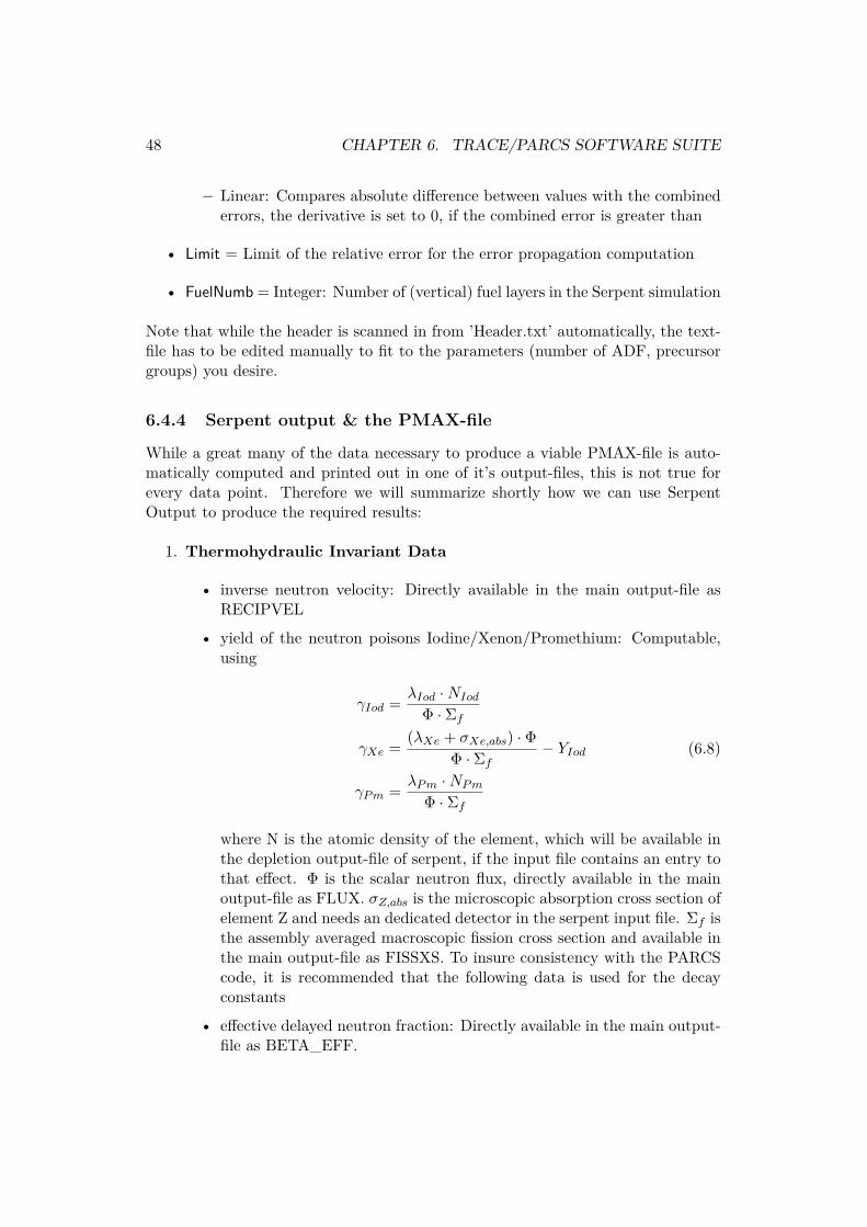
While a great many of the data necessary to produce a viable PMAX-file is auto-matically computed and printed out in one of it’s output-files, this is not true forevery data point. Therefore we will summarize shortly how we can use SerpentOutput to produce the required results:
1. Thermohydraulic Invariant Data
• inverse neutron velocity: Directly available in the main output-file asRECIPVEL
• yield of the neutron poisons Iodine/Xenon/Promethium: Computable,using
γIod = λIod ·NIod
Φ · Σf
γXe = (λXe + σXe,abs) · ΦΦ · Σf
− YIod
γPm = λPm ·NPm
Φ · Σf
(6.8)
where N is the atomic density of the element, which will be available inthe depletion output-file of serpent, if the input file contains an entry tothat effect. Φ is the scalar neutron flux, directly available in the mainoutput-file as FLUX. σZ,abs is the microscopic absorption cross section ofelement Z and needs an dedicated detector in the serpent input file. Σf isthe assembly averaged macroscopic fission cross section and available inthe main output-file as FISSXS. To insure consistency with the PARCScode, it is recommended that the following data is used for the decayconstants
• effective delayed neutron fraction: Directly available in the main output-file as BETA_EFF.

6.4. PARCS AND THE PMAX-FILE FORMAT 49
Table 6.1: decay constants of neutron poisons
Isotope λ135Xe 2.09167 · 10−5
135I 2.89500 · 10−5
135Pm 3.55568 · 10−6
• decay constant of delayed neutrons: Directly available in the main output-file as DECAY_CONSTANT.
2. Reference Data Block
• transport cross section: Directly available in the main output-file asTRANSPXS.
• absorption cross section: Directly available in the main output-file asABSXS.
• fission neutron production cross section: Directly available in the mainoutput-file as NSF.
• fission energy production cross section: Product of fission cross sectionFISSXS and energy release per fission event FISSE (plus a constant factorto transform MeV into W).
• microscopic xenon cross section: Available in the detector ouput file(s)when an dedicated detector is written in the serpent input file.
• microscopic samarium cross section: Available in the detector ouputfile(s) when an dedicated detector is written in the serpent input file.
• fission cross section: Directly available in the main output-file as FISSXS.• detector response parameter: Not available, kept original values.• scattering cross section: Directly available in the main output-file as
GTRANSFXS.• assembly discontinuity factor: Directly available in the main output-file
as ADFS.• corner discontinuity factor: Directly available in the main output-file as
ADFC.


Chapter 7
TRACE/PARCS Simulation
7.1 Description of SimulationAs already discussed on page 20, we perform a TRACE/PARCS simulation in threesteps. To recapitulate:
1. Flow SimulationSimulation with fixed power level and PARCS neutronics deactived, serves tofind a stable equilibrium with the given reactor geometry. Produces one tracedump-file which is reused as restart-file for the steady state computation.
2. Steady State SimulationSimulation with fixed power level but activated reactivity feedbacks and neu-tronics, serves to find a stable equilibrium with the given fuel cross-sections.Produces one TRACE and one PARCS dump-file both of which are reused asrestart-files for the transient computation. Used to check the power distribu-tion, resulting from our PMAX-files and fuel distribution.
3. Transient SimulationThe power level is calculated by PARCS neutronics. Standard procedure isrun the transient simulation for 20 seconds of in-simulation time, confirmingthe stability of the steady state, before activating the actual transient.
7.1.1 Accident Scenario
The model is based on the Ringhals I BWR Reactor. We simulate a turbine trip at65% of full power (this corresponds to 1475.5 MWth). A malfunction of a turbineor reactor system causes an abrupt stop of the steamflow from the main circuit(immediate shut-down of the turbine control valve), resulting in a pressure wave inthe primary circuit. It is possible for the pressure wave to damage valves and othercontrol elements. In our case, we will assume the failure of the bypass-valve, whichcould discharge steam directly into the condensor. We consider two scenarios forCR-behaviour:
51

52 CHAPTER 7. TRACE/PARCS SIMULATION
1. SCRAM (= Safety Control Rod Axe Man)CR are shoot into the reactor hydraulically and are fully inserted within 3.8seconds.
• Turbine trip: triggered after 25.0 seconds in-simulation time.• SCRAM: CR will be triggered if any of three control conditions is meet:
Power output rises to 10 % or more over steady state levels. Pressurein the steamdome to 10% or more over steady state levels. More thanone second has passed since the turbine trip. The CR will be completelyinserted within 3.8 seconds.
• Pump shut down: Pumps are controlled by the same set of triggerconditions as the SCRAM, but with an additional time delay of onesecond. The impeller continues to wind down for another 120 seconds.
• Valves: Turbine and Feedwater valve are controlled by the same setof trigger conditions as the SCRAM and shut down with a time delayof 0.0 seconds and 2.0 seconds, respectively. The Bypass valve fails toopen.
• ADS: Safety relief system for overpressure in the reactor vessel, consist-ing of three banks of valves, triggering at 7.90 · 106Pa (26.6 % of totalarea), 8.02 · 106Pa (26.6 % of total area), 8.20 · 106Pa (46.8 % of totalarea). All valves close at 7.86 · 106Pa.
2. Screw inThe hydraulic system fails and CR are screwed in mechanically. The triggersignal is received at the same time as in 1, but time to full insertion is 260seconds. In all other aspects this simulation is identical to the SCRAM.
The scenario was chosen to study the effects of extreme oscillations in modera-tor density, expected in a turbine trip, might have on the reactivity in a reactor,containing hafnium-cladding and MOX-fuel.

7.2. RESULTS: STEADY STATE CONVERGENCE 53
7.2 Results: Steady State convergenceIn this section we want to compare the steady state results, and their convergence,of the new fuel configurations to the results yielded by the original cross sections.
Table 7.1: Steady State values comparison
Parameter OrgXS Config.2 Config.2HiAc: 12.50 HiAc: 15.00
Reactor Power 1475.5 1475.5 1475.5in MW(th)Steamdome Pressure 7.02 7.02 7.02in MPaFeedwater mass flow 692.49 692.70 692.43in kg/sSteamline mass flow 692.94 693.13 692.90in kg/s
Temperature: Feedwater 425.83 425.96 425.80in KelvinTemperature: Steamline 558.99 558.99 558.99in Kelvin
Void fraction in % 45.44 42.26 45.95
0 200 400 600 800 1000
Time (s)
1e+09
1.5e+09
2e+09
2.5e+09
3e+09
Pow
er (
W)
HiAc1500
HiAc1250
OrgXS
Figure 7.1: Steady State: Power Output

54 CHAPTER 7. TRACE/PARCS SIMULATION
200 400 600 800 1000
Time (s)
630
640
650
660
670
680
690
700M
ass
Flo
w (
kg/s
)
OrgXS: Steamline
OrgXS: Feedwater
HiAc1250: Steamline
HiAc1250: Feedwater
HiAc1500: Steamline
HiAc1500: Feedwater
Figure 7.2: Steady State: In-&Outflows
0 200 400 600 800
Time (s)
7.017e+06
7.018e+06
7.019e+06
7.02e+06
7.021e+06
Ste
amdo
me
Pre
ssur
e (P
a)
HiAc1250
HiAc1500
OrgXS
Figure 7.3: Steady State: Steamdome Pressure

7.2. RESULTS: STEADY STATE CONVERGENCE 55
Figure 7.4: Steady State: Radial power distribution for OrgXS
Axial power distribution for the steady state computations can be found in Figure5.1 on page 32. Short overview of the relevant data:
Table 7.2: Steady State Power Peaking Comparison
Maximal Power OrgXS Config.2 Config.2Peaking Factor HiAc: 12.50 HiAc: 15.00
Radial 1.7050 1.5742 1.5112
Axial 2.2753 1.5205 2.1008

56 CHAPTER 7. TRACE/PARCS SIMULATION
Figure 7.5: Steady State: Radial power distribution for HiAc1250
Figure 7.6: Steady State: Radial power distribution for HiAc1500

7.3. RESULTS: TRANSIENT 57
7.3 Results: TransientThe fuel vector employed in these simulations is balancing precariously on the edgeof a positive void worth, ’Config. 1’ may have failed because of the concentrationof TRU-elements in the upper quarter and the resulting increase in relative weightof fast fission reactions.The simulation tries to negotiate a compromise between enough moderation to allowfor negative void worth and a hard enough neutron spectrum to produce a noticeableHA burn-up.
7.3.1 Presentation of Results: SCRAM, core-wide variables
We simulate the accidents described above for original cross sections of the Ringhals-1 (abbreviated as "OrgXS") and configuration 2 with a TRU-content of 16.48%and relative HA-contents of 12.50% and 15.00% (abbreviated as "HiAc1250" and"HiAc1500", respectively).Our model employs 25 fuel layers, plus one layer of reflectors below and above theactive core, plus a layer of ’upper plenum’. The first fuel containing layer is A02,the last A26. Displaying 25 data streams per fuel would mfake the graph entirelyunreadable, therefore we limit ourselves to between 3 to 5 data streams per reactorloading, which should be sufficient to at least show the most important trends.To make the plots immediately identifiable we will use black to denote data froma simulation with the original cross sections, red for data from Config.2 with arelative TRU content of 15.00%, navy blue for data from Config.2 with a relativeTRU content of 12.50%. Where necessary, different line styles are used to indicatethe z-coordinates of the plot. Where this results in incomprehensible plots, we willintroduce additional colours, zoom in or reduce the amount of displayed data, asthe situation warrants. Deviations form this color scheme are usually noted in theaccompanying text, but if in doubt the reader is adviced to check the legend.All (z-dependent) channel data is taken at the hot channel of the core.The first part will only contain variables, which are independent of the z-coordinateof the core.

58 CHAPTER 7. TRACE/PARCS SIMULATION
0 50 100 150
Time (s)
0
5e+08
1e+09
1.5e+09
2e+09P
ower
(W
)
OrgXs Power
HiAc_1500
HiAc_1250
Figure 7.7: Power output of all fuel config. during SCRAM
24 26 28 30 32
Time (s)
0
5e+08
1e+09
1.5e+09
2e+09
Pow
er (
W)
OrgXs
HiAc_1500
HiAc_1250
Figure 7.8: Zoom: Power output of all fuel config. during SCRAM

7.3. RESULTS: TRANSIENT 59
0 50 100 150 200 250 300
Time (s)
7e+06
7.2e+06
7.4e+06
7.6e+06
7.8e+06
8e+06
Pre
ssur
e (P
a)
OrgXs SteamDomePressure
HiAc_1500 SteamDomePressure
HiAc_1250 SteamDomePressure
Figure 7.9: Steam dome pressure of all fuel config. during SCRAM
20 30 40 50 60 70
Time (s)
7e+06
7.2e+06
7.4e+06
7.6e+06
7.8e+06
8e+06
Pre
ssur
e (P
a)
OrgXs SteamDomePressure
HiAc_1500 SteamDomePressure
HiAc_1250 SteamDomePressure
Figure 7.10: Zoom: Steam dome pressure of all fuel config. during SCRAM

60 CHAPTER 7. TRACE/PARCS SIMULATION
0 50 100 150 200 250 300
Time (s)
0
100
200
300
400
500
600
700
Ma
ss F
low
(kg
/s)
OrgXS ADS
OrgXS Steamline
OrgXS Feedwater
HiAc_1500 ADS
HiAc_1500 Steamline
HiAc_1500 Feedwater
HiAc_1250 ADS
HiAc_1250 Steamline
HiAc_1250 Feedwater
Figure 7.11: Massflows from and to the core of all fuel config. during SCRAM
24 26 28 30 32
Time (s)
0
100
200
300
400
500
600
700
Ma
ss F
low
(kg
/s)
OrgXS ADS
OrgXS Steamline
OrgXS Feedwater
HiAc_1500 ADS
HiAc_1500 Steamline
HiAc_1500 Feedwater
HiAc_1250 ADS
HiAc_1250 Steamline
HiAc_1250 Feedwater
Figure 7.12: Zoom: Massflows from and to the core of all fuel config. during SCRAM

7.3. RESULTS: TRANSIENT 61
0 50 100 150 200 250 300
Time (s)
5
6
7
8
9
Le
ng
th (
m)
OrgXs DowncomerLevel
HiAc_1500 DowncomerLevel
HiAc_1250 DowncomerLevel
Figure 7.13: Water level in Downcomer of all fuel config. during SCRAM
Figure 7.14: Maximum fuel temp. in the core of all fuel config. during SCRAM

62 CHAPTER 7. TRACE/PARCS SIMULATION
7.3.2 Presentation of Results: SCRAM, z-coord.-dependentvariables
0 50 100 150 200 250 300
Time (s)
0
200
400
600
800
De
nsi
ty (
kg/m
^3)
OrgXsA04
OrgXsA16
OrgXsA26
HiAc_1500 A04
HiAc_1500 A16
HiAc_1500 A26
HiAc_1250 A04
HiAc_1250 A16
HiAc_1250 A26
Figure 7.15: Mixture Density of Coolant for all fuel config. during SCRAM
0 50 100 150 200 250 300
Time (s)
720
740
760
780
De
nsi
ty (
kg/m
^3)
OrgXsA04
OrgXsA16
OrgXsA26
HiAc_1500 A04
HiAc_1500 A16
HiAc_1500 A26
HiAc_1250 A04
HiAc_1250 A16
HiAc_1250 A26
Figure 7.16: Zoom: Mixture Density of Coolant for all fuel const. during SCRAM

7.3. RESULTS: TRANSIENT 63
0 50 100 150 200 250 300
Time (s)
7e+06
7.2e+06
7.4e+06
7.6e+06
7.8e+06
8e+06P
ress
ure
(Pa)
OrgXsA04
OrgXsA16
OrgXsA26
HiAc_1500 A04
HiAc_1500 A16
HiAc_1500 A26
HiAc_1250 A04
HiAc_1250 A16
HiAc_1250 A26
Figure 7.17: Pressure all fuel config. during SCRAM
0 50 100 150 200 250 300
Time (s)
7.64e+06
7.66e+06
7.68e+06
7.7e+06
7.72e+06
7.74e+06
Pre
ssur
e (P
a)
OrgXsA04
OrgXsA16
OrgXsA26
HiAc_1500 A04
HiAc_1500 A16
HiAc_1500 A26
HiAc_1250 A04
HiAc_1250 A16
HiAc_1250 A26
Figure 7.18: Zoom: Pressure for all fuel config. during SCRAM

64 CHAPTER 7. TRACE/PARCS SIMULATION
0 50 100 150 200 250 300
Time (s)
0
0.2
0.4
0.6
0.8
ga
s vo
lum
e f
ract
ion
OrgXSA04
OrgXSA16
OrgXSA26
HiAc_1500 A04
HiAc_1500 A16
HiAc_1500 A26
HiAc_1250 A04
HiAc_1250 A16
HiAc_1250 A26
Figure 7.19: Void fraction for all fuel config. during SCRAM
25 30 35 40 45 50
Time (s)
0
0.2
0.4
0.6
0.8
ga
s vo
lum
e f
ract
ion
OrgXSA04
OrgXSA16
OrgXSA26
HiAc_1500 A04
HiAc_1500 A16
HiAc_1500 A25
HiAc_1250 A04
HiAc_1250 A16
HiAc_1250 A26
Figure 7.20: Zoom: Void fraction for all fuel config. during SCRAM

7.3. RESULTS: TRANSIENT 65
7.3.3 Presentation of Results: Reactivity
Reactivity plots will not use the colour-scheme described on page 57.
Figure 7.21: Reactivity: Original Cross Sections
Figure 7.22: Reactivity: Config. 2 with 16.48 % TRU, 15.00 % of which are HA

66 CHAPTER 7. TRACE/PARCS SIMULATION
Figure 7.23: Reactivity: Config. 2 with 16.48 % TRU, 12.50 % of which are HA
7.3.4 Discussion of SCRAM Results
To reiterate shortly, we have searched for a configuration that combined a maximumpossible burn-up of higher actinides with the given stability constraints of the axialpower profile. Config.1 and others were considered and discarded for instability.Finally Config.2 was choosen with a TRU-concentration of 16.48 %, to emulate asclosely as possible the optimal configuration found in [12], and an absolute HA-content of 2.06% (12.50% relative to the TRU-content) and 2.472% (15.00% rela-tive). A coupled TRACE/PARCS simulation was performed for this set-up and theaccident scenario described on page 51. The original cross sections were kept toserve as a baseline.Upon the shutdown of the turbine valve the power output of the reactor growsthe fastest for the original fuel loading and the slowest for Config.2 with 2.06%HA-content (12.50% relative), see Figure 7.8. Comparing the reactivity reactions,caused by the change in coolant density, which is a result of the closing turbinevalve, shutting down the steamline and thereby the outflow of coolant from thereactor, we get Figure 7.24.We observe a strongly positive density coolant reactivity introduction for the originalcross sections and negative reactivity introductions for the Config.2 cross sectionswith 12.50% and 15.00% HA-content.We find the reason for this in the collapsing void fraction, visible in Figure 7.19, andthe attendant rise in moderator density (see: Figure 7.15) caused by rising pressureinside the reactor vessel (see: Figure 7.17), which in turn is caused by continued

7.3. RESULTS: TRANSIENT 67
Figure 7.24: Coolant Density Reactivity: All Configurations
heating of the coolant by the fuel rods. The void collapse turns the coolant densitycontribution to the reactivity positive, due to increased moderation for the originalcross sections and negative for the Config.2 cross sections.The positive reactivity peaks at 27.02 s for HiAc-1500 and 29.35 s HiAc-1250, onthe other hand, are somewhat counterintuitive.For a possible explanation, it is worth remembering that, although the introductionof hafnium in the cladding will impoverish the thermal end of the neutron spectrum,thermal neutrons will still contribute to the chain reaction, especially in the lowerregions of the reactor. 239Pu, for example, has a considerable thermal fission crosssection and fission probability. In fact it might be possible that a fast neutron,escaping the fuel pin, would have a greater chance of inducing a fission event, if itgets moderated below the energy interval of ca 10,000 to 5 eV (see: Figure 1.7),where the resonance peaks of hafnium are located, before it reenters a fuel pin.Coolant continues to be pushed into the reactor for two seconds, after the turbinevalve has closed, first reaching the lower fuel strata, where the increased moderationhas an overall positive effect, then progressing upwards, see Figures 7.19, 7.15 and7.16, where the effect turns negative due to an increased reliance on fast neutronsto maintain the chain reaction.As the coolant density reactivity is the dominant reactivity factor, neglecting for themoment the control rod contribution, the difference in behaviour, described above,account for a majority of the differences in power growth, with the speed of power

68 CHAPTER 7. TRACE/PARCS SIMULATION
increase (see: Figure 7.8) reflecting the coolant density reactivity.As already discussed, the rise in pressure is caused by the energy deposited in thecoolant from the fuel rods, evaporating the water, and the lack of an outlet of thegrowing amount of steam.The pressure rise is not primarily influenced by the speed of the power peak, as afaster rising power curve will simply trigger the control rods earlier (trigger condi-tions, see: page 51), but by the absolute amount of energy absorbed by the coolant,which can be thought of as the area under the power curve (see: Figure 7.8). ThusConfig.2 with 12.50 % HA, although in possession of the slowest power rise of allconsidered configurations, causes the fastest increase in pressure (see: Figure 7.10).If the pressure exceeds 7.90 MPa the first bank of ADS-Valves is triggered andsteam is released from the steamdome, until the pressure drops to 7.86 MPa orlower. This process causes a characteristic, sharp jag in the curve, as steam is firstreleased to the containment and then replaced by the evaporation of coolant due tolower pressure in the reactor vessel and continued heating by the fuel rods.To illustrate, we plot the pressure for all considered configurations together withthe ADS-Outflow in one graph.
20 25 30 35 40 45 50
Time (s)
7e+06
7.2e+06
7.4e+06
7.6e+06
7.8e+06
8e+06
Pre
ssur
e (P
a)
OrgXsA04
OrgXsA10
OrgXsA16
OrgXsA22
OrgXsA26
HiAc_1500 A04
HiAc_1500 A10
HiAc_1500 A16
HiAc_1500 A22
HiAc_1500 A26
HiAc_1250 A04
HiAc_1250 A10
HiAc_1250 A16
HiAc_1250 A22
HiAc_1250 A26
0
100
200
300
400
Ma
ss F
low
(kg
/s)
ADS: MassFlow HiAc_1250
Figure 7.25: Compare: Pressure for all fuel config. during SCRAM and ADS-Massflow
Notice that the original cross sections and Config.2 with 15.00 % HA cross sections,whose ADS-valves stayed closed during the simulation, also miss the characteristicform.

7.3. RESULTS: TRANSIENT 69
5000
10000
15000
20000
delta
Pre
ssur
e (P
a)
delta Pressure @ SteamSep
0 50 100 150 200 250 300
Time (s)
-1000
0
1000
2000
3000
4000
Ma
ss F
low
(kg
/s)
MassFlow through SteamSep
Figure 7.26: Compare: Pressure difference and MassFlows in Steam Seperator
It should be noted that the pressure oscillations, prominently visible in Figure 7.18,have an entirely different origin. A pressure difference builds between the intake ofthe steam seperator and the outlet in the upper end of the downcomer, driven bythe heating of the coolant in the reactor core. When the pressure difference growsan increasing amount of steam/water-mixture is sucked into the steam seperator,this flushes relatively cool condensate out of the lower end of the downcomer intothe core, where it contributes to cooling and thereby lowering the pressure, resultingin the oscillatory form we observe in the aforementioned figures.This effect is also visible in the downcomer level (see: Figure 7.13) and the mixturedensity (see: Figures 7.15 to 7.16). We plot the pressure difference and resultingmass flow in Figure 7.26. Note that the graphs are phase-shifted by approximatelya quarter wave-length, which would be the expected relation of an oscillation andit’s driving force.

70 CHAPTER 7. TRACE/PARCS SIMULATION
7.3.5 Presentation of Results: Scew-in, core-wide variables
100 200 300 400
Time (s)
0
1e+09
2e+09
3e+09
4e+09
Pow
er (
W)
OrgXS
HiAc_1500
HiAc_1250
Figure 7.27: Power output, all fuel config. during screw in
20 40 60 80
Time (s)
0
1e+09
2e+09
3e+09
4e+09
Pow
er (
W)
OrgXS
HiAc_1500
HiAc_1250
Figure 7.28: Zoom: Power output, all fuel config. during screw in

7.3. RESULTS: TRANSIENT 71
100 200 300 400
Time (s)
7e+06
7.2e+06
7.4e+06
7.6e+06
7.8e+06
8e+06
8.2e+06
Pre
ssur
e (P
a)
OrgXs
HiAc_1250
HiAc_1250
Figure 7.29: Steam dome pressure, all fuel config. during screw in
20 40 60 80
Time (s)
7e+06
7.2e+06
7.4e+06
7.6e+06
7.8e+06
8e+06
8.2e+06
Pre
ssur
e (P
a)
OrgXs
HiAc_1250
HiAc_1250
Figure 7.30: Zoom: Steam dome pressure, all fuel config. during screw in

72 CHAPTER 7. TRACE/PARCS SIMULATION
20 25 30 35 40
Time (s)
0
100
200
300
400
500
600
700M
ass
Flo
w (
kg/s
)
OrgXS: Steamline
OrgXS: Feedwater
HiAc_1500: Steamline
HiAc_1500: Feedwater
HiAc_1250: Steamline
HiAc_1250: Feedwater
Figure 7.31: Zoom: Massflows from and to the core, Feedwater&Steamline all fuelconfig.
0 50 100 150 200 250
Time (s)
0
200
400
600
800
1000
Ma
ss F
low
(kg
/s)
OrgXS: ADS
HiAc_1500: ADS
Figure 7.32: Zoom: HiAc1500 ADS-Massflow, during screw in

7.3. RESULTS: TRANSIENT 73
0 50 100 150 200 250
Time (s)
0
200
400
600
800
1000
Ma
ss F
low
(kg
/s)
OrgXS: ADS
HiAc_1250: ADS
Figure 7.33: Zoom: HiAc1250 ADS-Massflows, during screw in
0 100 200 300 400
Time (s)
5
6
7
8
9
Le
ng
th (
m)
OrgXS
HiAc_1500
HiAc_1250
Figure 7.34: Water level in Downcomer, all fuel config. during screw in

74 CHAPTER 7. TRACE/PARCS SIMULATION
0 100 200 300
Time (s)
500
1000
1500
2000
Ma
x F
ue
l T
em
pe
ratu
re [
°K]
OrgXs
HiAc_1500
HiAc_1250
Figure 7.35: Max. fuel temp. in the core, all fuel config. during screw in
7.3.6 Presentation of Results: Screw in, z-coord.-dependentvariables
0 100 200 300 400 500
Time (s)
0
200
400
600
800
De
nsi
ty (
kg/m
^3)
OrgXs A02
OrgXs A08
OrgXs A20
OrgXs A26
HiAc_1250 A02
HiAc_1250 A08
HiAc_1250 A20
HiAc_1250 A26
HiAc_1500 A02
HiAc_1500 A08
HiAc_1500 A20
HiAc_1500 A26
Figure 7.36: Mixture Density of Coolant, all fuel config. during screw in

7.3. RESULTS: TRANSIENT 75
20 40 60 80 100 120 140
Time (s)
0
200
400
600
800
De
nsi
ty (
kg/m
^3)
OrgXs A02
OrgXs A08
OrgXs A20
OrgXs A26
HiAc_1250 A02
HiAc_1250 A08
HiAc_1250 A20
HiAc_1250 A26
HiAc_1500 A02
HiAc_1500 A08
HiAc_1500 A20
HiAc_1500 A26
Figure 7.37: Zoom: Mixture Density of Coolant, all fuel config. during screw in
0 100 200 300 400 500
Time (s)
0
0.2
0.4
0.6
0.8
ga
s vo
lum
e f
ract
ion
OrgXS A02
OrgXS A08
OrgXS A20
OrgXS A26
HiAc_1250 A02
HiAc_1250 A08
HiAc_1250 A20
HiAc_1250 A26
HiAc_1500 A02
HiAc_1500 A08
HiAc_1500 A20
HiAc_1500 A26
Figure 7.38: Void fraction, all fuel config. during screw in

76 CHAPTER 7. TRACE/PARCS SIMULATION
20 40 60 80 100 120 140
Time (s)
0
0.2
0.4
0.6
0.8
1
ga
s vo
lum
e f
ract
ion
OrgXS A02
OrgXS A08
OrgXS A20
OrgXS A26
HiAc_1250 A02
HiAc_1250 A08
HiAc_1250 A20
HiAc_1250 A26
HiAc_1500 A02
HiAc_1500 A08
HiAc_1500 A20
HiAc_1500 A26
Figure 7.39: Zoom: Void fraction, all fuel config. during screw in
7.3.7 Presentation of Results: Reactivity during screw in
Reactivity plots will not use the colour-scheme described on page 57.
Figure 7.40: Reactivity: Original Cross Sections

7.3. RESULTS: TRANSIENT 77
Figure 7.41: Reactivity: Config.2 with 16.48% TRU, 15.00% of which are HA
Figure 7.42: Reactivity: Config.2 with 16.48% TRU, 12.50% of which are HA

78 CHAPTER 7. TRACE/PARCS SIMULATION
7.3.8 Discussion of Screw-In Results
Power, Reactivity, Moderator Density & ADS MassflowThe power graph in Figure 7.28 shows a prominent peak structure, which we canrediscover in the reactivity graphs Figure 7.40 to 7.42. Cause is the changing steamdischarge through the ADS over-pressure valve, see Figure 7.32 and Figure 7.33.Note the step-like shape of the discharge curve, each step corresponding to theopening of another valve bank (trigger conditions, see: page 51).To illustrate we plot massflow through the ADS-valves into one graph, togetherwith the corresponding power output, see Figures 7.43 to 7.45.The original cross section data set is the most obvious example, but not the onlyone. The covariance between ADS-massflow and power is visible in Config. 2 withboth fuel loadings.Notice that the while the following plots cover only the time interval 0 to 250seconds, they do, in fact, extend over the full 400 seconds but were pruned of thelast 150, uneventful seconds, to provide better resolution in the visible time interval.Plotting reactor power next to ADS-outflow:
50 100 150 200
Time (s)
0
1e+09
2e+09
3e+09
4e+09
Pow
er (
W)
OrgXS: Power
0
200
400
600
800
Ma
ss F
low
(kg
/s)
OrgXS: ADS Massflow
Figure 7.43: OrgXS: Compare power output & ADS massflow

7.3. RESULTS: TRANSIENT 79
50 100 150 200
Time (s)
0
5e+08
1e+09
1.5e+09
2e+09
Pow
er (
W)
HiAc_1500: Power
0
200
400
600
800
Ma
ss F
low
(kg
/s)
HiAc1500: ADS MassFlow
Figure 7.44: Config.2, 15.00% HA: Compare power output & ADS massflow
50 100 150 200
Time (s)
0
5e+08
1e+09
1.5e+09
2e+09
Pow
er (
W)
HiAc_1250: Power
0
200
400
600
800M
ass
Flo
w (
kg/s
)
HiAc1250: ADS MassFlow
Figure 7.45: Config.2, 12.50% HA: Compare power output & ADS massflow

80 CHAPTER 7. TRACE/PARCS SIMULATION
We can follow the causlity chain backwards through our plot results: power changeswith introduced reactivity, which changes with CR movement and moderator den-sity, which is influenced by the periodic steam discharges from the ADS-valve.To test this theory we plot z-coord-dependent mixture density, with increased z-wiseresolution, and ADS-massflow in one graph and get:
50 100 150 200 250
Time (s)
200
400
600
De
nsi
ty (
kg/m
^3)
OrgXsA04
OrgXsA10
OrgXsA16
OrgXsA19
OrgXsA22
OrgXsA25
OrgXsA28
0
200
400
600
800
Ma
ssfl
ow
(kg
/s)
OrgXs: ADS Massflow
Figure 7.46: OrgXS: Compare ADS massflow & av. Mod. Density

7.3. RESULTS: TRANSIENT 81
Zoom in on 50 to 100 second-intervall:
50 60 70 80 90
Time (s)
200
400
600
De
nsi
ty (
kg/m
^3)
OrgXsA04
OrgXsA10
OrgXsA16
OrgXsA19
OrgXsA22
OrgXsA25
OrgXsA28
0
200
400
600
800
Ma
ssfl
ow
(kg
/s)
OrgXs: ADS Massflow
Figure 7.47: OrgXS, Zoom: Compare ADS massflow & av. Mod. Density
Identical plots for Config.2, 12.50% HA:
0 100 200 300 400
Time (s)
0
200
400
600
800
De
nsi
ty (
kg/m
^3)
HiAc_1250 A02
HiAc_1250 A04
HiAc_1250 A06
HiAc_1250 A08
HiAc_1250 A10
HiAc_1250 A12
HiAc_1250 A14
HiAc_1250 A16
HiAc_1250 A18
HiAc_1250 A20
HiAc_1250 A22
HiAc_1250 A24
HiAc_1250 A25
HiAc_1250 A26
0
200
400
600
800
Ma
ssfl
ow
(kg
/s)
HiAc1250: ADS MassFlow
Figure 7.48: Config.2, 12.50% HA: Compare ADS massflow & av. Mod. Density

82 CHAPTER 7. TRACE/PARCS SIMULATION
Zoom in on 50 to 100 second-intervall:
50 100 150 200
Time (s)
0
200
400
600
800
De
nsi
ty (
kg/m
^3)
HiAc_1250 A14
HiAc_1250 A16
HiAc_1250 A18
HiAc_1250 A20
HiAc_1250 A22
HiAc_1250 A24
HiAc_1250 A25
HiAc_1250 A26
0
100
200
300
Ma
ssfl
ow
(kg
/s)
HiAc1250: ADS MassFlow
Figure 7.49: Config.2, 12.50% HA, Zoom: Comp. ADS massflow & av. Mod. Dens.
It should be obvious from Figures 7.43 to 7.45 that closing the ADS-valve coincideswith a power peak, although we cannot realiably conclude cause and effect from thisalone. We skip this type of plot for the remaining fuel configurations and continuewith the change of reactivity with moderator density, averaged over the z-axis:
400
500
600
700
800
De
nsi
ty (
kg/m
^3)
HiAc1500: Average Density
OrgXS: Average Density
0 100 200 300 400 500
Time (s)
0
5
10
15
20
Re
act
ivity
($
)
HiAc1500: Density-Coolant-Reactivity
OrgXS: Density-Coolant-Reactivity
Figure 7.50: Config.2, 15.00% HA: Compare DC-Reactivity & av. Mod. Density

7.3. RESULTS: TRANSIENT 83
400
500
600
700
800
De
nsi
ty (
kg/m
^3)
HiAc1500: Average Density
OrgXS: Average Density
120 140 160 180 200 220 240
Time (s)
0
5
10
15
20
Re
act
ivity
($
)
HiAc1500: Density-Coolant-Reactivity
OrgXS: Density-Coolant-Reactivity
Figure 7.51: Config.2, 15.00% HA, Zoom: Comp. DC-Reactivity & av. Mod. Dens.
Reactivity and average moderator density plot for Config. 2, HA-content of 12.50% and original cross sections.
400
500
600
700
800
De
nsi
ty (
kg/m
^3)
HiAc1250: Average Density
OrgXS : Average Density
0 100 200 300 400
Time (s)
0
5
10
15
20
Co
ola
nt
De
nsi
ty R
ea
ctiv
ity
($)
HiAc1250: Density Coolant Reactivity
OrgXS : Density Coolant Reactivity
Figure 7.52: Config.2, 12.50% HA: Compare DC-Reactivity & av. Mod. Density

84 CHAPTER 7. TRACE/PARCS SIMULATION
Zoom in on 100 to 250 second-intervall:
400
500
600
700
800
De
nsi
ty (
kg/m
^3)
HiAc1250: Average Density
OrgXS : Average Density
100 150 200 250
Time (s)
0
5
10
15
20
Co
ola
nt
De
nsi
ty R
ea
ctiv
ity
($)
HiAc1250: Density Coolant Reactivity
OrgXS : Density Coolant Reactivity
Figure 7.53: Config.2, 12.50% HA, Zoom: Comp. DC-Reactivity & av. Mod. Dens.
Analyzing the enlarged graphs in Figures 7.51 and 7.53, we notice that for the OrgXSdensity coolant reactivity oscillates in phase with averaged moderator density overthe length of the time intervall.Configuration 2 with 15.00 % HA and 12.50 % HA stays in phase with the densitycurve only upto, approximately, 150 to 170 seconds, followed by a period of non-alignement, lasting until the 200 second mark, approximately. At this point therelation between density and reactivity has inverted, a local minimum in densitywill coincide with a local maximum of the coolant density reactivity.The oscillations, caused by ADS-valve behaviour are overlaid on a global trend ofrising reactivity, running parallel to rising coolant density, until reaching a triggerpoint, where the coolant density reactivity of all fuel configurations, containing HA,takes a dive.Considering the reactivity plots Figure 7.40 to 7.42 we notice that the reactivityworth of the control rods is mirroring the behaviour of DC-reactivity along x-axis,until it reaches the trigger point and sharply declines. It is worth noting, thateven the OrgXS exhibit this CR-worth behaviour, meaning it is likely a function ofthe reactor set-up and not the fuel. On page 66 we suspected that, TRU-contentnotwithstanding, the chain reaction was still relying on thermal neutrons, especiallyin the lower reaches of the core. This theory gains credibility with the results of thescrew-in. Increasing moderator density causes a parallel growth in DC-reactivity-worth, indicating a continued dominance of thermal neutrons.The sudden drop of DC-worth for the Config. 2, with both HA-concentrations,

7.3. RESULTS: TRANSIENT 85
seems to indicate a critical point at which the sum of the contributions of fast andthermal neutrons becomes negative. Most likely due to a combination of a risinglevel of high density moderater (see: Figures 7.46 and 7.52) - note that the collapsein DC-worth coincides exactly with the last rise of mixture density, before reachingit’s maximum value, in the topmost fuel layer (see Figures 7.54 and 7.55 ) - and therising control rod hardening the neutron spectrum.Comparing the DC-induced reactivities in Figure 7.56 we notice the slower ascent ofthe HA-containing fuels, followed by the sharp drop-off to a positive void coefficientfor Config. 2.
0
200
400
600
800
De
nsi
ty (
kg/m
^3)
HiAc1500: Density A25
HiAc1500: Density A26
0 100 200 300 400 500
Time (s)
0
2
4
6
8
10
12
Re
act
ivity
($
)
HiAc1500: Density-Coolant-Reactivity
Figure 7.54: Config.2, 15.00% HA; Compare: Moderator Density in upper fuel layers& DC-Reactivity

86 CHAPTER 7. TRACE/PARCS SIMULATION
200
300
400
500
600
700
De
nsi
ty (
kg/m
^3)
HiAc1250: Density A26
HiAc1250: Density A25
0 100 200 300 400 500
Time (s)
0
2
4
6
8
10
12R
ea
ctiv
ity (
$)
HiAc1250: Density-Coolant-Reactivity
Figure 7.55: Config.2, 12.50% HA; Compare: Moderator Density in upper fuel layers& DC-Reactivity
Comparison of DC-induced reactivity for all configurations:
Figure 7.56: Coolant Density Reactivity: All Configurations

7.3. RESULTS: TRANSIENT 87
Pressure, Void Fraction, DensityIn the paragraph above, we noted the growth of the coolant density for all fuelconfigurations and it’s effect on the reactivity and consequently the power outputduring the shutdown. The change in coolant density is caused by the collapse of thevoid fraction, see Figure 7.38, which is due to the sharply rising pressure, see Figure??, which in turn rises the boiling point of the fluid and compresses the steam intothe steam dome. During the transient the maximum pressure is limited to 8.2 MPaby the opening of the ADS-valve, resulting in a raise of the saturation temperatureby more than 10 K from it’s steady state value at ca. 559 K.The saw-like form of the pressure-graph is a result of the pressure-triggered ADS-valve, releasing steam to the containment. The pressure spikes can be found as localgas fraction minima or density maxima in Figures 7.37 and 7.39, respectively. Themid-sized pressure arks for Config. 3, with 12.50% HA,are especially well visible,both in the density and the gas fraction plot, in layer A20, between 35 and 70 sec-onds.Figure ?? shows more pressure spike, with a higher frequency, for the mainly UOXcontaining fuels, as a result of the positive reactivity feedback, from the highermoderator density.
Waterlevel & Heat FluxThe original cross sections produce higher fuel temperatures than fuel configura-tions with HA-content, although a rising HA-content also correlates with risingtemperatures, see Figure 7.35. Consequently, in the same coolant supply, this leadsto higher pressures during shut down, see Figure 7.18, and a higher loss of coolant,see Figure 7.34. A possible reason for the higher retention of water in the case ofHiAc_1500 might be the more bottom heavy power distribution, see Figure 5.1. Asthe CR get inserted from the bottom, this leads to a faster "relative" shut down.The active part of the core extends to 4.40 m and stays covered by more than halfa meter of water in all cases. Waterlevels after the screw-in:
• OrgXS: 5.28 m
• HiAc_1500: 5.51 m
• HiAc_1250: 5.43 m
• Config_1: 5.42 m
Another security relevant variable would be the critical heat flux, which is the max-imum amount of energy per second and square meter a fuel rod can emit before thewater-filme, covering it, evaporates, severly limiting the ability of the fuel rod toshed heat. This is known as dry-out and the resulting spike in cladding temperaturecan damage the fuel rod, constrict the coolant flow and, in extreme cases, cause aself-reinforcing process that results in a core-melt.
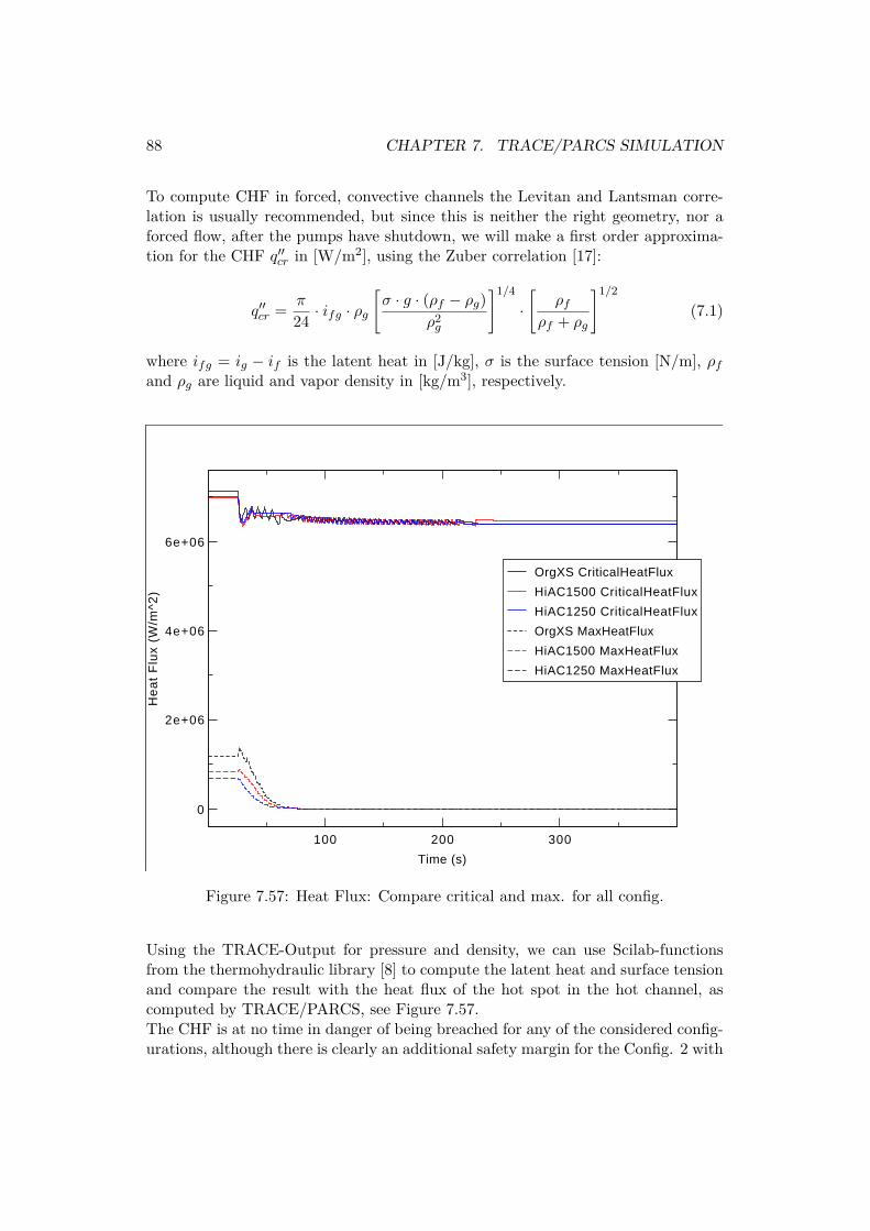
88 CHAPTER 7. TRACE/PARCS SIMULATION
To compute CHF in forced, convective channels the Levitan and Lantsman corre-lation is usually recommended, but since this is neither the right geometry, nor aforced flow, after the pumps have shutdown, we will make a first order approxima-tion for the CHF q′′cr in [W/m2], using the Zuber correlation [17]:
q′′cr = π
24 · ifg · ρg[σ · g · (ρf − ρg)
ρ2g
]1/4
·[
ρfρf + ρg
]1/2
(7.1)
where ifg = ig − if is the latent heat in [J/kg], σ is the surface tension [N/m], ρfand ρg are liquid and vapor density in [kg/m3], respectively.
100 200 300
Time (s)
0
2e+06
4e+06
6e+06
He
at
Flu
x (W
/m^2
)
OrgXS CriticalHeatFlux
HiAC1500 CriticalHeatFlux
HiAC1250 CriticalHeatFlux
OrgXS MaxHeatFlux
HiAC1500 MaxHeatFlux
HiAC1250 MaxHeatFlux
Figure 7.57: Heat Flux: Compare critical and max. for all config.
Using the TRACE-Output for pressure and density, we can use Scilab-functionsfrom the thermohydraulic library [8] to compute the latent heat and surface tensionand compare the result with the heat flux of the hot spot in the hot channel, ascomputed by TRACE/PARCS, see Figure 7.57.The CHF is at no time in danger of being breached for any of the considered config-urations, although there is clearly an additional safety margin for the Config. 2 with

7.4. CONCLUSIONS 89
12.50% HA, which is owed mostly to lower fuel temperatures of this configuration.
7.4 ConclusionsWe notice that increased hafnium content, while increasing the TRU-content in amanner to keep keff constant will decrease the HA-burn-up. A higher HA-contentof the TRU, will allow us to regain the lost ground but will decrease the maximalpossible burn-up.Concentration of the TRU in the upper reaches of the core will maximize burn-up,but not yield a stable configuration, needed to complete a Trac/PARCS simulation.The accident scenario studied here, responds well to the introduction of HA-enrichedMOX-fuel. Config. 2 is stable and adhering to safety restrictions, concerning axialpower distribution, core uncovering or dry-out are even less a danger for the HA-containing fuel, than for the original fuel loading.The rising pressure, caused by the continued heating from the fuel elements, resultsin a void collapse, which progresses upwards through the core, until reaching thetopmost fuel layer at ca. 220 to 230 seconds.This corresponds approximately to the transitional period during the shut-down, inwhich an increase in moderator density contributes positively to the reactivity inthe TRU-loaded core (or to put it otherwise: in which the void coefficient is overallnegative), although less so than an identical increase in density would contribute inthe UOX-fueled core, which is used as a baseline.For the present accident scenario this circumstance serves to suppress power spikesduring the screw-in, examples which are observable for the original cross sectionsimulation. Although the final value of DC-reactivity is increasingly negative withhigher HA-content, indicating a positve overall void coefficient, the long lead time,until it takes full effect, may give hope to proponents of HA-burning in BWR. Ina hypothetical loss of coolant scenario, the transitional period might allow the safeshut-down of the reactor, although further study in this matter is to be recom-mended.


Chapter 8
Appendix A
91

92 CHAPTER 8. APPENDIX A
Table 8.1: Summary of HA & Pu burn-upGeometry Config. 1 Config. 2 Config. 3 Config. 4TRU [%] 16.48 16.48 16.48 16.48HA [%] 2.06 (12.5%) 2.06 (12.5%) 2.06 (12.5%) 2.06 (12.5%)Hf [%] 0.05 0.05 0.05 0.05
Elements HA Pu HA Pu HA Pu HA Puburn-up in 0.62412 19.0472 0.56008 18.9117 0.52780 18.7154 0.55243 18.6935kg/TWh/tFuelGeometry Config. 2 Config. 2 Config. 2 Config. 2TRU [%] 16.48 21.30 27.50 32.00HA [%] 2.06 (12.5%) 2.6625 (12.5%) 3.4375 (12.5%) 4.000 (12.5%)Hf [%] 0.05 0.05 0.10 0.15
Elements HA Pu HA Pu HA Pu HA Puburn-up in 0.56008 18.9117 0.22980 22.6157 -0.31578 26.1206 -0.81042 28.5554kg/TWh/tFuelGeometry Config. 2 Config. 2 Config. 2 Config. 2TRU [%] 18.20 23.30 29.40 34.00HA [%] 2.730 (15%) 3.495 (15%) 4.410 (15%) 5.100 (15%)Hf [%] 0.05 0.05 0.10 0.15
Elements HA Pu HA Pu HA Pu HA Puburn-up in 1.95066 18.4096 1.6894 22.1530 0.72362 15.7337 0.27822 14.9851kg/TWh/tFuelGeometry Config. 2 Config. 2 Config. 2 Config. 2TRU [%] 16.48 21.30 27.50 32.00HA [%] 2.472 (15%) 3.195 (15%) 4.125 (15%) 4.800 (15%)Hf [%] 0.05 0.05 0.10 0.15
Elements HA Pu HA Pu HA Pu HA Puburn-up in 1.71238 17.3726 1.56663 21.0901 1.14372 24.4566 0.90545 26.6435kg/TWh/tFuelGeometry Config. 2 Config. 2 Config. 2 Config. 2TRU [%] 22.30 27.50 33.30 38.00HA [%] 4.460 (20%) 5.500 (20%) 6.660 (20%) 7.600 (20%)Hf [%] 0.05 0.05 0.10 0.15
Elements HA Pu HA Pu HA Pu HA Puburn-up in 4.52881 18.0199 4.34981 21.3072 2.64078 16.1119 2.06981 15.4459kg/TWh/tFuel

Bibliography
[1] "World Energy Outlook 2009" commissioned by the International EnergyAgency; designed and directed by Birol, Fatih
[2] Ålander, Alexandra; Dufek, Jan; Gudowski, Waclaw; "From once-throughnuclear fuel cycle to accelerator driven transmutation"; Nuclear Instrumentsand Methods in Physics Research; 2006
[3] Nuclear Energy Agency (NEA); "Actinide and Fission Product Partioning andTransmutation", OCED Publications
[4] International Atomic Energy Agency (IAEA); Implications of Partioning andTransmutation in Radioactive Waste Management; Technical Report SeriesNo. 435
[5] Wallenius, Janne; "Transmutation of nuclear waste" course notes available athttp://www.neutron.kth.se/courses/transmutation/lecturenotes.shtml
[6] Wakabayashi, T.; Ohki, S.; Ikegami, T.; "Feasibility sutdies of an optimisedreactor core for minor actinide and fission product transmutation"; Int. Conf.Evaluation of Emerging Nuclear Fuel Cycles Systems; Versailles, France; 1995
[7] Wallenius, Janne; Westlen, Daniel; "Hafnium clad fuels for fast spectrumBWRs"; Annals of Nuclear Energy 35 (2008) 60-67
[8] Thermohydraulic libraries for Scilab, available athttp://www.reactor.sci.kth.se/downloads/
[9] LeppÃďnen, J.; "Development of a New Monte Carlo Reactor Physics Code.";D.Sc. Thesis, Helsinki University of Technology (2007)
[10] LeppÃďnen, J.; Pusa, M; "Computing the matrix exponential in Burn-UpCalculations"; Nuclear Science and Engineering; 2009
[11] Sutton, T. M.; "Wielandt Iteration as Applied to the Nodal ExpansionMethod"; Nuclear Science and Engineering; 98, pp. 169-173 (1988)
[12] Suvdantstseg, M.; "Optimisation of safety coefficients in BWR transmuta-tion"; Ms. Sc. Thesis, Stockholm Royal Institute of Technology; 2009
93

94 BIBLIOGRAPHY
[13] Downar, T.; Kozlowski, T.; Lee, D.; Xu, Y.; "PARCS v2.6 U.S. NRC CoreNeutronics Simulator - Theory Manual", School of Nuclear Engineering, Pur-due University
[14] Bajorek, S.; Gavrilas, M.; Gingrich, C.; "TRACE V4.160 User’s Manual",United States Nuclear Regulatory Commission
[15] Downar, T.; Xu, Y.; "Code for generating the PARCS Cross Section InterfaceFile PMAXS", School of Nuclear Engineering, Purdue University
[16] Arobio, A.; "Optimisation of the void worth in a Boiling Water Reactor withhafnium cladding"; Ms. Sc. Thesis, Stockholm Royal Institute of Technology;2010
[17] Anglart, H; "Thermal-Hydraulics in Nuclear Systems", Course script; 2010
[18] Dinh, T; Kozlowski, T; Roshan, S; "Development of RELAP5/PARCS coupledcode models for the safety analysis of Oskarshamn-3 BWR plant", StockholmRoyal Institute of Technology; 2006