Research ArticleTransient Pressure Behavior of Complex Fracture Networks inUnconventional Reservoirs

Gou Feifei,1 Liu Chuanxi,1 Ren Zongxiao ,2,3 Qu Zhan,2,3 Wang Sukai,4 Qin Xuejie,1

Fang Wenchao,1 Wang Ping,2,3 and Wang Xinzhu2,3

1State Key Laboratory of Shale Oil and Gas Enrichment Mechanisms and Effective Development, China2College of Petroleum Engineering, Xi’an Shiyou University, Xi’an 710065, China3Xi’an Shiyou University Shanxi Key Laboratory of Well Stability and Fluid & Rock Mechanics in Oil and Gas Reservoirs, China4Engineering Technology Research Institute Xibu Drilling Engineering Company, Karamay 834000, China

Correspondence should be addressed to Ren Zongxiao; 765802228@qq.com

Received 15 May 2021; Revised 5 June 2021; Accepted 12 October 2021; Published 3 November 2021

Academic Editor: Jianchao Cai

Copyright © 2021 Gou Feifei et al. This is an open access article distributed under the Creative Commons Attribution License,which permits unrestricted use, distribution, and reproduction in any medium, provided the original work is properly cited.

Unconventional resources have been successfully exploited with technological advancements in horizontal-drilling and multistagehydraulic-fracturing, especially in North America. Due to preexisting natural fractures and the presence of stress isotropy, severalcomplex fracture networks can be generated during fracturing operations in unconventional reservoirs. Using the DVSmethod, a semianalytical model was created to analyze the transient pressure behavior of a complex fracture network inwhich hydraulic and natural fractures interconnect with inclined angles. In this model, the complex fracture network canbe divided into a proper number of segments. With this approach, we are able to focus on a detailed description of thenetwork properties, such as the complex geometry and varying conductivity of the fracture. The accuracy of the newmodel was demonstrated by ECLIPSE. Using this method, we defined six flow patterns: linear flow, fracture interferenceflow, transitional flow, biradial flow, pseudoradial flow, and boundary response flow. A sensitivity analysis was conductedto analyze each of these flow regimes. This work provides a useful tool for reservoir engineers for fracture designing aswell as estimating the performance of a complex fracture network.

1. Introduction

Technological advances in horizontal-drilling and multistagehydraulic-fracturing have stimulated a boom in unconven-tional resource generation throughout the world, especiallyin North America. Because of the presence of stress isotropyand preexisting natural fractures, complicated fracture net-works can be created in unconventional reservoirs when con-ducting stimulation treatments [1, 2] (Fisher et al., 2002;Maxwell et al., 2002). Knowledge of the fluid flow behaviorin these complex fracture networks is essential informationto evaluate the performance and effectiveness of stimulation.

Several models have been established by scholars to pre-dict the behavior of fracture networks in unconventional res-ervoirs in the last decade. These models can be divided intothree categories. The first category is the analytical method,

based on the well-known dual-porosity model [3, 4] (War-ren and Root, 1963; Kazemi, 1969), which is comprised ofthe fracture network and surrounding matrix. Analyticalmodels [5–9] (Brown et al.,2011; Ozkan et al.,2011; Xuet al.,2013; Leng et al.,2014; Ting et al.,2015) were developedto investigate the transient pressure behavior of multistagefractured horizontal wells on the basis of the dual-porosityhypothesis. These analytic models have helped engineersgain a comprehensive insight into the performance of frac-ture networks and have provided practical tools to evaluatestimulation effectiveness. However, the fracture network isvery complex, and the dual-porosity medium may not rigor-ously capture the details of the fracture network characteris-tics, such as the irregular spatial distribution, complexinterconnected scenarios, and conductivity heterogeneity ofthe fractures.

HindawiGeofluidsVolume 2021, Article ID 6273822, 11 pageshttps://doi.org/10.1155/2021/6273822

The second category is semianalytical and was developedusing the method of source function [10, 11] (Zhao et al.,2014; Pin et al.,2015). In these models, the complex fracturenetwork can be divided into a proper number of segments.This approach allows one to focus on a detailed descriptionof the network properties and overcomes the shortcomingsof the analytical method. Yet, these semianalytical modelscannot accurately simulate the fluid flow in a reservoir.These semianalytical models assume that the fluid flow inthe reservoir is 2D in an infinite plate reservoir, and thesource function cannot consider the effects of fracture geom-etry. We show an approach that can overcome these short-comings in the model described below.

The third category is numerical simulation, in whichthe hydraulic and natural fractures are usually representedby high permeability refined grids [12–14] (Palagi andAziz,1994; Skoreyko and Peter,2003; Li et al.,2003). Basedon a structured grid system in conventional numerical simu-lators [15–17], Mayerhofer et al. (2010), Warpinski et al.(2008), and Cipolla (2009) simulated the production oforthogonal networks in shale gas reservoirs. These worksqualitatively analyzed how the size and density, fracture con-ductivity, matrix permeability, and gaps in fracture networksaffect the horizontal well productivity. However, the numer-ical methods are time-consuming and have inherent uncer-tainties that could cause them to be less accurate.

In view of this, there is still lack of an efficient and rigor-ous approach to model the flow behavior of complex frac-ture networks in unconventional reservoirs. The mainobjective of this paper is to develop a semianalytical modelthat can evaluate the performance of such networks morerigorously and efficiently compared to the existing methods.This new model is based on the DVS (distributed volumesources) method [18] (Valko et al. 2007), in which the frac-tures in the network are explicitly represented by discretesegments to concentrate on the details of the network char-acteristics, such as the complex geometry and varying con-ductivity. The DVS model can simulate fluid flow in aclosed boundary reservoir in 3D. The accuracy of the newmodel was demonstrated by ECLIPSE. Then, using thismethod, we defined the flow patterns of the fluid in the res-ervoir and conducted a sensitivity analysis of the transientpressure behavior.

2. Establishment of the Theoretical Model

First, we describe the fracture network used to introduce ourapproach and then provide the mathematic model for thereservoir and fracture flow.

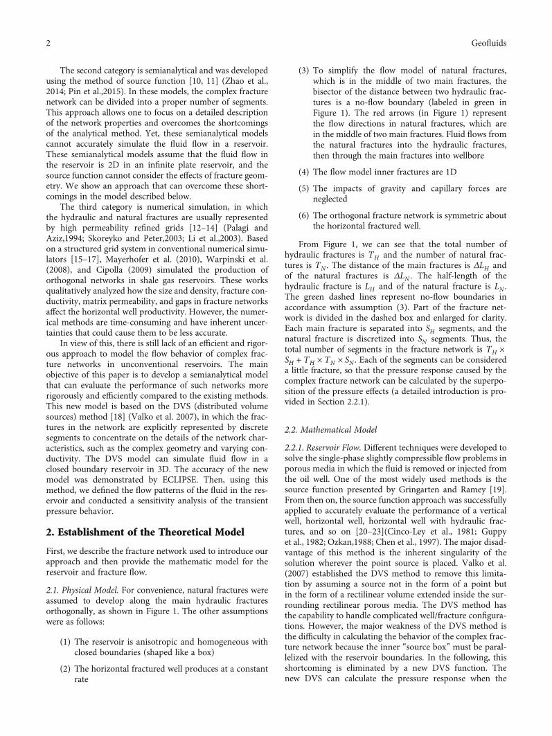
2.1. Physical Model. For convenience, natural fractures wereassumed to develop along the main hydraulic fracturesorthogonally, as shown in Figure 1. The other assumptionswere as follows:

(1) The reservoir is anisotropic and homogeneous withclosed boundaries (shaped like a box)

(2) The horizontal fractured well produces at a constantrate

(3) To simplify the flow model of natural fractures,which is in the middle of two main fractures, thebisector of the distance between two hydraulic frac-tures is a no-flow boundary (labeled in green inFigure 1). The red arrows (in Figure 1) representthe flow directions in natural fractures, which arein the middle of two main fractures. Fluid flows fromthe natural fractures into the hydraulic fractures,then through the main fractures into wellbore

(4) The flow model inner fractures are 1D

(5) The impacts of gravity and capillary forces areneglected

(6) The orthogonal fracture network is symmetric aboutthe horizontal fractured well.

From Figure 1, we can see that the total number ofhydraulic fractures is TH and the number of natural frac-tures is TN . The distance of the main fractures is ΔLH andof the natural fractures is ΔLN . The half-length of thehydraulic fracture is LH and of the natural fracture is LN .The green dashed lines represent no-flow boundaries inaccordance with assumption (3). Part of the fracture net-work is divided in the dashed box and enlarged for clarity.Each main fracture is separated into SH segments, and thenatural fracture is discretized into SN segments. Thus, thetotal number of segments in the fracture network is TH ×SH + TH × TN × SN . Each of the segments can be considereda little fracture, so that the pressure response caused by thecomplex fracture network can be calculated by the superpo-sition of the pressure effects (a detailed introduction is pro-vided in Section 2.2.1).

2.2. Mathematical Model

2.2.1. Reservoir Flow. Different techniques were developed tosolve the single-phase slightly compressible flow problems inporous media in which the fluid is removed or injected fromthe oil well. One of the most widely used methods is thesource function presented by Gringarten and Ramey [19].From then on, the source function approach was successfullyapplied to accurately evaluate the performance of a verticalwell, horizontal well, horizontal well with hydraulic frac-tures, and so on [20–23](Cinco-Ley et al., 1981; Guppyet al., 1982; Ozkan,1988; Chen et al., 1997). The major disad-vantage of this method is the inherent singularity of thesolution wherever the point source is placed. Valko et al.(2007) established the DVS method to remove this limita-tion by assuming a source not in the form of a point butin the form of a rectilinear volume extended inside the sur-rounding rectilinear porous media. The DVS method hasthe capability to handle complicated well/fracture configura-tions. However, the major weakness of the DVS method isthe difficulty in calculating the behavior of the complex frac-ture network because the inner “source box” must be paral-lelized with the reservoir boundaries. In the following, thisshortcoming is eliminated by a new DVS function. Thenew DVS can calculate the pressure response when the

2 Geofluids

surfaces of the fracture have inclined angles with the reser-voir boundary’s directions.

(1) Valko’s (2007) DVS Model. First, the main principle ofValko’s (2007) DVS method will be introduced. A schematicof Valko’s (2007) DVS is shown in Figure 2. The reservoir ishomogeneous with closed boundaries (box-shaped). Theinner “source box” is assumed to be a smaller rectilinearbox with surfaces parallel to the reservoir boundaries (forsimplicity, the inner “source box” can be considered a littlefracture).

As shown in Figure 2, the geometry of this model isdescribed with the following parameters: reservoir dimen-

sions in the x, y, and z directions (xe, ye, and ze, respec-tively); reservoir permeability along the principal axes (kx ,ky, and kz); coordinates of the center point of the source(cx, cy , and cz); and half-lengths of the source in the x, y,and z directions (wx, wy, and wz , respectively). The mathe-matical model for the volume source in closed boundarieswas established by Valko et al. (2007) and is shown inAppendix A.

The pressure response of a rectilinear reservoir withclosed boundaries for an instantaneous withdrawal fromthe volume source was given by Valko (2007) and is as fol-lows (the definitions of the dimensionless variables areshown as Appendix B):

Using Equation (1), we obtained a 3D solution of theinstantaneous pressure response in anisotropic reservoirswhere the permeability along the three axes is different fromeach other (kx, ky, and kz). In addition, contrary to Gringar-ten’s source function, Equation (1) can take the dimensionof volume source (2wx, 2wy, and 2wz) into account.

(2) Establishment of the New DVS Model. The presence ofvolume source surfaces in the x − y plane, which are not par-

allel to the reservoir boundaries, is a common occurrence incomplex fracture networks. The schematic for this case isshown in Figure 3.

The inclined angle between the volume source and the x-axis is denoted as θx. The endpoint coordinates of theinclined source are (cx1, cy1) and (cx2, cy2). The cx coordinateof the center line for a particular volume source (labeled bluedashed line in Figure 3) is a constant when θx = 90o. At other

∆LH

∆LN

1

234

5678

::

1 2 3 4 5 6 7 8 ...

Hydraulic fracture number is TH

Horizontal wellN

atur

al fr

actu

re n

umbe

r is T

N

No flow boundary

LNLHSH

SN

Figure 1: Physical model and discretized fracture segments of a complex fracture network.

pδD xD, yD, zD, tDð Þ = 1 + 〠∞

n=1

sin nπ cxD +wxDð Þ − sin nπ cxD −wxDð Þ2nπwxD

cos nπxDe−n2π2 kx/kð Þ L/xeð Þ2tD

" #

× 1 + 〠∞

n=1

sin nπ cyD +wyD

� �− sin nπ cyD −wyD

� �2nπwyD

cos nπyDe−n2π2 ky/kð Þ L/yeð Þ2tD

" #

× 1 + 〠∞

n=1

sin nπ czD +wzDð Þ − sin nπ czD −wzDð Þ2nπwzD

cos nπzDe−n2π2 kz /kð Þ L/zeð Þ2tD

" #:

ð1Þ

3Geofluids

angles, the cx coordinate of the center line is a function of y.As shown in Equation (A.4), cx is a term in the Heavisideunit-step function. The role of the Heaviside unit-step func-tion in Equation (A.1) is to limit the position and geometryof the volume source. Therefore, the solution form for thevolume source surfaces that are not parallel to reservoir

boundaries is the same as that in Equation (1), with the addi-tion of a formula to calculate cx (shown as Equation (2)).

The geometrical relationship between cx and y is pre-sented as follows.

cx =cx1 + y − cy1

� �/tan θx, θx ≠

π

2cx1, θx =

π

2 :

8><>: ð2Þ

Figure 4 shows the case in which the volume sourceforms an angle θy with the y-axis.

The geometrical relationship between cy and x is similarto Equation (2) and is as follows.

cy =cy1 + x − cx1ð Þ/tan θy , θy ≠

π

2cy1, θy =

π

2 :

8><>: ð3Þ

Therefore, the pressure response for an instantaneouswithdrawal from a volume source, which can have arbitrarilyangle (in x/y or both x and y directions), is given as follows:

xyz

xe

ze

ye

2wx 2wy2wz

(cy,cz)

(cx,cy)

(cy,cz)

Figure 2: Schematic of the volume source in closed boundaries.

x

y

(cx1, cy1)

(cx2, cy2)

2wy

2wx

(cx, cy)𝜃y

Figure 4: The surface of volume source is not parallel to thereservoir boundaries.

x

y

(cx1, cy1)

(cx2, cy2)

(cx, cy)2wy

2wx

𝜃x

Figure 3: The surface of the volume source is not parallel to thereservoir boundaries.

pδD xD, yD, zD, tDð Þ = 1 + 〠∞

n=1

sin nπ cxD +wxDð Þ − sin nπ cxD −wxDð Þ2nπwxD

cos nπxDe−n2π2 kx/kð Þ L/xeð Þ2tD

" #

× 1 + 〠∞

n=1

sin nπ cyD +wyD

� �− sin nπ cyD −wyD

� �2nπwyD

cos nπyDe−n2π2 ky/kð Þ L/yeð Þ2tD

" #

× 1 + 〠∞

n=1

sin nπ czD +wzDð Þ − sin nπ czD −wzDð Þ2nπwzD

cos nπzDe−n2π2 kz/kð Þ L/zeð Þ2tD

" #,

ð4Þ

cxD =cxD1 + yD − cyD1

� �/tan θx, θx ≠

π

2cxD1, θx =

π

2 ,

8><>:

cyD =cyD1 + xD − cxD1ð Þ/tan θy , θy ≠

π

2cyD1, θy =

π

2 :

8><>:

ð5Þ

4 Geofluids

From Equations (4) and (5) generalized the forms ofValko’s solution, which is specific condition when θ = 90ois presented.

To obtain the response of the reservoir for a continuousvolume source, we numerically integrate the pressure deriv-ative solution over time:

pD xD, yD, zD, tDð Þ = qD

ðtD0pδD xD, yD, zD, τð Þdτ: ð6Þ

As for the complex fracture network, shown in Figure 1,each segment can be considered a volume source; therefore,the total number of volume sources is

NT = TH × SH + TH × TN × SN : ð7Þ

The pressure response at any point in the reservoir (orinside the fracture network) can be calculated by superimpos-ing the source function of the NT segments. Thus, the dimen-sionless pressure of fracture i can be obtained as follows.

pDi = 〠n=NT

j=1qDjpDi,j: ð8Þ

In Equation (8), qDj represents the source strength of thesegment j, and pDi,j represents the dimensionless pressure cal-culated at the center of segment i if the source is placed in seg-ment j.

Applying Equation (8) to all of the fracture segments inthe fracture network, NT equations are obtained.

2.2.2. Fracture Flow Model. Following assumptions (3) and(4), the flow model was established for the fracture network.According to (Gringarten, et al. 1974; Cinco-Ley et al., 1988)[24, 25], the diffusivity equation in the fractures can bedescribed as follows.

kfμ

∂2pf∂x2

+qfwf h

= 0: ð9Þ

The initial condition is

pf���t=0

= pi: ð10Þ

The inner boundary condition is

pf���x=0

= pw: ð11Þ

The outer boundary condition is

∂pf∂x

����x=LH

= 0: ð12Þ

With the definitions for the dimensionless variables (seeAppendix B), the above equations can be adapted as follows:

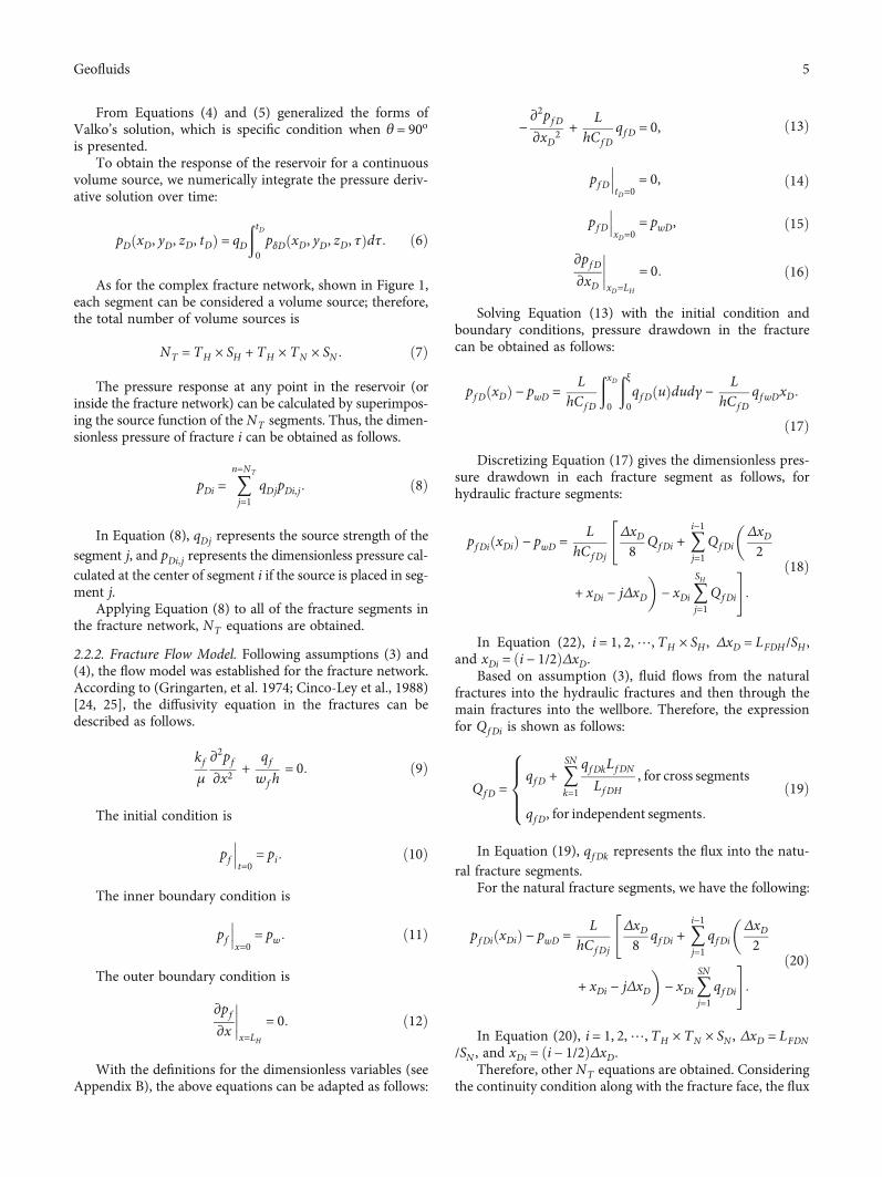
−∂2pfD∂xD2 + L

hCfDqfD = 0, ð13Þ

pfD���tD=0

= 0, ð14Þ

pfD���xD=0

= pwD, ð15Þ

∂pfD∂xD

����xD=LH

= 0: ð16Þ

Solving Equation (13) with the initial condition andboundary conditions, pressure drawdown in the fracturecan be obtained as follows:

pfD xDð Þ − pwD = LhCfD

ðxD0

ðξ0qfD uð Þdudγ − L

hCfDqfwDxD:

ð17Þ

Discretizing Equation (17) gives the dimensionless pres-sure drawdown in each fracture segment as follows, forhydraulic fracture segments:

pfDi xDið Þ − pwD = LhCfDj

"ΔxD8 QfDi + 〠

i−1

j=1QfDi

�ΔxD2

+ xDi − jΔxD

�− xDi 〠

SH

j=1QfDi

#:

ð18Þ

In Equation (22), i = 1, 2,⋯, TH × SH , ΔxD = LFDH/SH ,and xDi = ði − 1/2ÞΔxD.

Based on assumption (3), fluid flows from the naturalfractures into the hydraulic fractures and then through themain fractures into the wellbore. Therefore, the expressionfor QfDi is shown as follows:

QfD =qfD + 〠

SN

k=1

qfDkLfDN

LfDH, for cross segments

qfD, for independent segments:

8>><>>: ð19Þ

In Equation (19), qfDk represents the flux into the natu-ral fracture segments.

For the natural fracture segments, we have the following:

pfDi xDið Þ − pwD = LhCfDj

"ΔxD8 qfDi + 〠

i−1

j=1qfDi

�ΔxD2

+ xDi − jΔxD

�− xDi 〠

SN

j=1qfDi

#:

ð20Þ

In Equation (20), i = 1, 2,⋯, TH × TN × SN , ΔxD = LFDN/SN , and xDi = ði − 1/2ÞΔxD.

Therefore, other NT equations are obtained. Consideringthe continuity condition along with the fracture face, the flux

5Geofluids

and pressure should satisfy the following condition:

pfDi = pDi,qfDi = qDi:

ð21Þ

The assumption of constant production rate requires

〠NT

i=1qfDi = 1: ð22Þ

Currently we have obtained 2NT + 1 equations fromEquations (8), (18), (20), and (22). Similarly, there are 2NT+ 1 unknowns, including pwD, qDi, and pDi. Using theGauss-Jordan elimination, the pwD can be obtained by simul-taneously solving the system of equations.

3. Results and Discussion

3.1. Model Validation. The accuracy of this new model wasverified using ECLIPSE (Schlumberger 2010). The orthogo-nal fracture network for the simulation included four mainhydraulic fractures and four natural fractures (similar toFigure 1). The grid scale in the simulation was 161 × 161 ×10, and the volume of the reservoir was 1610 × 1610 × 10m3. Details for the parameters used in the calculations aresummarized in Table 1.

The results of the semianalytical model and ECLIPSE arecompared in Figure 5 (where dpD represents the derivativeof the dimensionless pressure pD). From the figure, it isobserved that there is a good agreement between our modeland the ECLIPSE results.

Type curves of the transient pressure behavior for thecomplex fracture network are shown in Figure 6. FromFigure 6, we can see that six main flow regimes can be recog-nized as follows:

Regime I is linear flow. As is commonly known, the typ-ical feature of this flow behavior is that the slope of thedimensionless derivative pressure is equal to 0.5.

Regime II is a relatively rare occurrence in the literature.Figure 6 shows that a “cave” occurs at the end of linear flow.Few published papers have discussed this phenomenon,although published work shows this “cave” phenomenon(Pin et al., 2015). To further examine the “cave” behavior,we conducted calculations to analyze this phenomenon inSection 2.2.1 (Figure 7). The results showed that this “cave”reflects the effects of interference between hydraulic frac-tures and natural fractures. Therefore, we denote this pro-cess as “fracture interference flow.”

Regime III is transitional flow, generally raised at the endof Regime II.

Regime IV is biradial flow, which can be recognized by aone-third slope of the dimensionless derivative pressure.

Table 1: Data used for semianalytical and numerical models.

Reservoir length, m 1610 Permeability of hydraulic fractures, D 28

Reservoir width, m 1610 Length of natural fractures, m 200

Reservoir thickness, m 10 Width of natural fractures, m 0.0028

Reservoir compressibility, MPa-1 0.00022 Permeability of natural fractures, D 28

Reservoir permeability, mD 0.1 Wellbore radius, m 0.15

Fluid viscosity, pas 0.001 Production rate, m3/d 0.5

Length of hydraulic fractures, m 200 Reservoir initial pressure, MPa 14.6

Width of hydraulic fractures, m 0.0028 Reservoir porosity 0.1

1.E–04

1.E–03

1.E–02

1.E–01

1.E+00

1.E+01

1.E–06 1.E–04 1.E–02 1.E+00 1.E+02

pD/d

pD

tD

Semi-analysis pDSemi-analysis dpD

Numerical pDNumerical dpD

Figure 5: Comparison of the semianalytic model and numericalresults.

1.E–04

1.E–03

1.E–02

1.E–01

1.E+00

1.E+01

1.E–06 1.E–04 1.E–02 1.E+00 1.E+02

pD/d

pD

tD

Semi-analysis pDSemi-analysis dpD

III

IIIIV

VVI

Figure 6: Flow regimes of the complex fracture network.

6 Geofluids

This regime has been observed by several other researchers(Zhao et al.,2013; Luo et al.,2014; Chen et al.,2015) [26–28].

Regime V is pseudoradial flow with the derivative pres-sure stabilized at a value of 0.5.

Regime VI is reservoir boundary response flow. In thisstage, transient pressure has spread to the outer closedboundaries. The dimensionless derivative pressure curvetilted up and converged to a straight line with unit slope.

3.2. Effect of Fracture Permeability

3.2.1. Effect of Varying the Natural Fracture’s Permeability.Fracture permeability is a key parameter for fractured wells.Here, the effect of fracture permeability on the behavior oftransient pressure and fluid flow regimes is evaluated. Weconsidered the permeability of the hydraulic fractures to beconstant and varied the natural fracture’s conductivity. Thecombinations of kfH and kfN are shown in Table 2.

The effect of natural fracture permeability on transientpressure response of the four formations is shown inFigure 7 (the following results are based on data fromTable 1).

From Figure 7, we can see that natural fracture perme-ability primarily affects the fracture interference flow. Largerpermeability values for the natural fracture corresponded toa deeper “cave” in the typical curve. This is a result of theincreasing permeability of natural fractures, causing largerfluid flow into natural fractures, leading to a stronger inter-ference between hydraulic fractures and natural fractures.This flow regime is a typical signature of transient pressurebehavior in complex fracture network.

Horizontal well

Hydraulic fractureNatural fracture

Figure 10: Sketch of unorthogonal fracture network.

200m300m500m

700m900m

1.E–04

1.E–03

1.E–02

1.E–01

1.E+00

1.E+01

1.E–06 1.E–04 1.E–02 1.E+00 1.E+02

pD/d

pD

tD

Figure 9: Comparison of type curves with different fracturegeometry.

pD/d

pD

tD

8D18D

28D58D

1.E–04

1.E–03

1.E–02

1.E–01

1.E+00

1.E+01

1.E–06 1.E–04 1.E–02 1.E+00 1.E+02

Figure 8: Comparison of dimensionless derivative pressure forfour cases.

Formation A dpDFormation B dpD

Formation C dpDFormation D dpD

pD/d

pD

tD

1.E–04

1.E–03

1.E–02

1.E–01

1.E+00

1.E+01

1.E–06 1.E–04 1.E–02 1.E+00 1.E+02

Figure 7: Comparison of dimensionless derivative pressure for thefour reservoirs.

Table 2: The combinations of kfH and kfN .

ReservoirsPermeability of

hydraulic fractures, DPermeability of

natural fractures, D

Formation A 28 1.4

Formation B 28 4.4

Formation C 28 8.8

Formation D 28 28

7Geofluids

3.2.2. The Permeability of the Complex Fracture Network IsHomogeneous. Assuming that the proppant is evenly distrib-uted throughout the network, it is suggested that the perme-ability of the complex network is homogeneous. The data inTable 1 were used in the following calculations. Four casesthat were investigated in which permeability of the fracturenetwork were 8D, 18D, 28D, and 58D. Figure 8 shows theeffect of fracture permeability on the transient responsebehavior of the complex network.

From Figure 8, we can see that the permeability of thecomplex fracture network only influences the pressureresponse in the early stages of the process.

3.3. Effect of the Complex Fracture network’s Geometry. Thegeometry of the fracture network also has an importantinfluence on the pressure response in unconventional reser-voirs. For simplicity, it was assumed that all of the fractureshave the same length. Five cases were considered in whichthe fracture lengths were equal to 200m, 300m, 500m,700m, and 900m individually. These values were chosento investigate the effect of the complex fracture network’sgeometry on the pressure behavior. The following resultsare based on the data in Table 1.

The results of Figure 9 indicate that the geometry of thefracture network primarily affects transitional flow, biradialflow, and pseudoradial flow. It had no significant effect onother flow regimes. With the increase of fracture length,the period of transitional flow is also increased, and the bira-dial flow and pseudoradial flow gradually faded out.

3.4. Unorthogonal Fracture Network. In this section, the tran-sient pressure behavior of unorthogonal fracture networks isinvestigated. Figure 10 shows a sketch of an unorthogonalfracture network used in the following calculation.

Figure 10 shows an unorthogonal complex fracture net-work that is composed of several fracture segments witharbitrary angles. From the dashed box in Figure 10, we cansee that the discretization is not perfect in the connectionof two fractures. There are gaps in the connections, because

the surface of the volume source must be a parallelogram.However, we assumed that the flow inside the fracture net-work was continuous. The permeability of hydraulic fracturewas set to 40D, and that of natural fracture was 10D. Thetotal length of the fracture network was 1000m, and theother pertinent data are listed in Table 1. The semianalyticmodel results were verified by the results of ECLIPSE(Schlumberger 2010), shown in Figure 11.

The comparison between numerical results and this newmodel is shown in Figure 11. The difference of the newmodel compared with ECLIPSE is relatively large in the earlyperiod. The reason for this difference may be a result ofassumption (3) and the imperfect connections between twofractures in our model, as mentioned above. Except for earlytimed, the semianalytical model matches very well with thenumerical results.

4. Conclusions

This paper provides a semianalytical model for the transientpressure behavior in unconventional reservoirs that have acomplex fracture network. The model is capable of simulat-ing the complex fracture network with varying conductivi-ties and complex geometry. Although most of the resultsand discussion have been restricted to an orthogonal frac-ture network, we have demonstrated that the approach canbe used for unorthogonal fracture networks in whichhydraulic and natural fractures interconnect with arbitraryinclined angles by direct comparison with numerical results.The following conclusions can be drawn:

(1) We present a more flexible DVS model based on thework by Valko. Then a semianalytic model wasestablished to describe transient pressure behaviorof complex fracture networks in unconventional res-ervoirs with closed boundaries. The accuracy of thenew model was demonstrated by comparison withnumerical results. In addition, the model used 3Dflow to simulate the reservoir flow (in Section 2.2.1)

Semi-analysis pDSemi-analysis dpD

Numerical pDNumerical dpD

1.E–04

1.E–03

1.E–02

1.E–01

1.E+00

1.E+01

1.E–06 1.E–04 1.E–02 1.E+00 1.E+02

pD/d

pD

tD

Figure 11: Comparison between numerical results and semianalysis results.

8 Geofluids

(2) The process of fluid flow in unconventional reser-voirs with complex network can be divided into sixflow regimes: linear flow, fracture interference flow,transitional flow, biradial flow, pseudoradial flow,and boundary response flow. Note that the “fractureinterference flow” is a new flow regime that requiresadditional work to more fully describe it. Throughthe research in Sections 2.2 and 3.3, we determinedthat the permeability of the complex fracture net-works has a significant influence on the fractureinterference flow regime

(3) The results of a sensitivity analysis show that the per-meability of the fractures significantly influences ear-lier stage fluid flow (linear flow and fractureinterference flow). The geometry of the fracture net-work primarily affects transitional flow, biradialflow, and pseudoradial flow (shown in Figure 9).

As shown in Figure 11, the model deviates slightly fromthe numerical results in unorthogonal fracture networks.However future work will be focused on the optimizationof the model for this case. Even so, the model is a useful toolto investigate the flow behavior of complex fracture net-works. With this essential knowledge, we can evaluate wellperformance and stimulation effectiveness in unconven-tional reservoirs.

Appendix

A. The diffusivity equation for the volumesource model is given by Valko et al. (2007)as follows.

ηx∂2p∂x2

+ ηy∂2p∂y2

+ ηz∂2p∂z2

+ 1ϕct

Q x, y, z, tð Þ = ∂p∂t

, ðA:1Þ

where ηi = ki/ϕμct , i = x, y, z:The initial condition is

p x, y, z, 0ð Þ = pi: ðA:2Þ

The closed boundary conditions are

∂p∂x

����x=0

= ∂p∂x

����x=xe

= 0,

∂p∂y

����y=0

= ∂p∂y

����y=ye

= 0,

∂p∂z

����z=0

= ∂p∂z

����z=ze

= 0:

ðA:3Þ

Qðx, y, z, tÞ in Equation (A.1) is the source functionwhich, for the instantaneous volume source, is written as

Q x, y, z, tð Þ = qB8wxwywz

δ tð Þ H x − cx −wxð Þ −H x − cx +wxð Þ½ �

× H y − cy −wy

� �−H y − cy +wy

� �� �× H z − cz −wzð Þ −H z − cz +wzð Þ½ �:

ðA:4Þ

In Equation (A.4), δðtÞ and HðxÞ represent the Diracdelta function and the Heaviside unit-step function, respec-tively. The Dirac delta function makes the source instantane-ity, and the Heaviside unit-step function limits the geometryof the source.

B. The dimensionless parameters are definedas follows:

pD = kLqμB

pi − pð Þ, ðB:1Þ

pfD = kLqμB

pi − pf

, ðB:2Þ

pwD = kLqμB

pi − pwð Þ, ðB:3Þ

qfD =qf L

qB, ðB:4Þ

CfD =kf wf

kL, ðB:5Þ

tD = k

ϕμctL2 t, ðB:6Þ

xD = xLyD = y

LzD = z

L, ðB:7Þ

cxD = cxxe, ðB:8Þ

cyD =cyye, ðB:9Þ

k = kxkykz� �1/3, ðB:10Þ

L = LxLyLz� �1/3

: ðB:11Þ

Nomenclature

xe: Length of reservoir in x direction, mye: Width of reservoir in y direction, mze: Height of reservoir in z direction, mL: Length, mw: Width, mc: Coordinate of midpoint of volume source, mk: Permeability, m2

TH : Total number of hydraulic fractures, integerTN : Total number of natural fractures, integerSH : Total segments of one hydraulic fracture, integerSN : Total segments of one natural fracture, integer

9Geofluids

pw: Wellbore pressure, Pap: Pressure, Papδ: Instantaneous pressure, PaNT : Total number of fracture segments, integerμ: Viscosity, MPash: Height of fracture in z direction, mq: Flow rate, m3/dt: Time, second.SubscriptsD: DimensionlessN: Natural fractureH: Hydraulic fracturef: Fracturei, j: Fracture segments number, integer.

Data Availability

Data is available when required.

Conflicts of Interest

The authors declare that they have no conflicts of interest.

Acknowledgments

This work is funded by the State Key Laboratory of Shale Oiland Gas Enrichment Mechanisms and Effective Develop-ment, National Natural Science Foundation of China (GrantNo. 51804258, 51974255, and 51874241), Natural ScienceBasic Research Program of Shaanxi Province (Grant No.2019JQ-807, 2020JM-544, 2018JM-5054), and the YouthInnovation Team of Shaanxi Universities.

References

[1] M. K. Fisher, C. A. Wright, B. M. Davidson et al., Integratingfracture mapping technologies to optimize stimulations in theBarnett Shale, Society of Petroleum Engineers, 2002.

[2] S. C. Maxwell, T. I. Urbancic, N. Steinsberger, and R. Zinno,Microseismic imaging of hydraulic fracture complexity in theBarnett Shale, Society of Petroleum Engineers, 2002.

[3] J. E. Warren and P. J. Root, “The behavior of naturally frac-tured reservoirs,” Society of Petroleum Engineers Journal,vol. 3, no. 3, pp. 245–255, 1963.

[4] H. Kazemi, “Pressure transient analysis of naturally fracturedreservoirs with uniform fracture distribution,” Society of Petro-leum Engineers Journal, vol. 9, no. 4, pp. 451–462, 1969.

[5] M. Brown, E. Ozkan, R. Raghavan, and H. Kazemi, “Practicalsolutions for pressure transient responses of fractured hori-zontal wells in unconventional Shale reservoirs,” Society ofPetroleum Engineers Journal, vol. 2, no. 3, pp. 235–245, 2011.

[6] E. Ozkan, M. Brown, R. Raghavan, and H. Kazemi, “Compar-ison of fractured horizontal well performance in tight sand andshale reservoirs,” SPE Reservoir Evaluation and Engineering,vol. 14, no. 2, pp. 248–259, 2011.

[7] B. X. Xu, M. Haghighi, X. F. Li, and D. Cooke, “Developmentof new type curves for production analysis in naturally frac-tured shale gas/tight gas reservoirs,” Journal of Petroleum Sci-ence and Engineering, vol. 105, no. 1, pp. 107–115, 2013.

[8] L. Tian, C. Xiao, M. Liu et al., “Well testing model for multi-fractured horizontal well for shale gas reservoirs with consid-eration of dual diffusion in matrix,” Journal of Natural Gas Sci-ence and Engineering, vol. 21, pp. 283–295, 2014.

[9] T. Huang, X. Guo, and F. Chen, “Modeling transient flowbehavior of a multiscale triple porosity model for shale gas res-ervoirs,” Journal of Natural Gas Science and Engineering,vol. 23, pp. 33–46, 2015.

[10] Y. L. Zhao, L. H. Zhang, J. X. Luo, and B. N. Zhang, “Perfor-mance of fractured horizontal well with stimulated reservoirvolume in unconventional gas reservoir,” Journal of Hydrol-ogy, vol. 512, pp. 447–456, 2014.

[11] P. Jia, L. Cheng, S. Huang, and H. Liu, “Transient behavior ofcomplex fracture networks,” Journal of Petroleum Science andEngineering, vol. 132, pp. 1–17, 2015.

[12] C. L. Palagi and K. Aziz, “Use of Voronoi grid in reservoir sim-ulation,” Society of Petroleum Engineers Journal, vol. 2, no. 2,pp. 69–77, 1994.

[13] F. Skoreyko and H. Peter, “Use of PEBI grids for complexadvanced process simulators,” in Paper SPE 79685-MS Pre-sented at the SPE Reservoir Simulation Symposium, TX, USA,2003.

[14] B. Li, Z. Chen, and G. Huan, “The sequential method for theblack-oil reservoir simulation on unstructured grids,” Journalof Computational Physics, vol. 192, no. 1, pp. 36–72, 2003.

[15] M. J. Mayerhofer, E. P. Lolon, N. R. Warpinski, C. L. Cipolla,D. Walser, and C. M. Rightmire, “What is stimulated reservoirvolume (SRV)?,” SPE Production & Operations, vol. 25, no. 1,pp. 89–98, 2010.

[16] N. R. Warpinski, M. J. Mayerhofer, M. C. Vincent, C. L.Cipolla, and E. P. Lolon, “Stimulating unconventional reser-voirs: maximizing network growth while optimizing fractureconductivity,” Journal of Canadian Petroleum Technology,vol. 48, no. 10, pp. 39–51, 2009.

[17] C. L. Cipolla, “Modeling production and evaluating fractureperformance in unconventional gas reservoirs,” Journal ofPetroleum Technology, vol. 61, no. 9, pp. 84–90, 2009.

[18] P. P. Valko and S. Amini, The method of distributed volumetricsources for calculating the transient and pseudosteady state pro-ductivity of complex well-fracture configurations, Society ofPetroleum Engineers, 2007.

[19] A. C. Gringarten and H. J. Ramey, “The use of source andGreen’s functions in solving unsteady-flow problems in reser-voirs,” Society of Petroleum Engineers Journal, vol. 13, no. 5,pp. 285–296, 1973.

[20] H. Cinco-Ley and V. F. Samaniego, “Transient pressure analy-sis for fractured wells,” Society of Petroleum Engineers Journal,vol. 33, no. 9, pp. 1749–1766, 1981.

[21] K. H. Guppy, H. Cinco-Ley, H. J. Ramey, and V. F. Samaniego,“Non-Darcy flow in wells with finite-conductivity vertical frac-tures,” Society of Petroleum Engineers Journal, vol. 22, no. 5,pp. 681–698, 1982.

[22] E. Ozkan, Performance of Horizontal Wells, PhD Dissertation,University of Tulsa, Tulsa, Oklahoma, 1988.

[23] C.-C. Chen and R. Rajagopal, “Amultiply-fractured horizontalwell in a rectangular drainage region,” Society of PetroleumEngineers Journal, vol. 2, no. 4, pp. 455–465, 1997.

[24] A. C. Gringarten, H. J. Ramey, and R. Raghavan, “Unsteady-state pressure distributions created by a well with a singleinfinite-conductivity vertical fracture,” Society of PetroleumEngineers Journal, vol. 14, no. 4, pp. 347–360, 1974.

10 Geofluids

[25] H. Cinco-Ley and H.-Z. Meng, Pressure transient analysis ofwells with finite conductivity vertical fractures in double poros-ity reservoirs, Society of Petroleum Engineers, 1988.

[26] Z. Chen, X. Liao, X. Zhao, S. Lv, and L. Zhu, A SemianalyticalApproach for Obtaining Type Curves of Multiple-FracturedHorizontal Wells with Secondary-Fracture Networks, Societyof Petroleum Engineers, 2016.

[27] Y.-l. Zhao, L.-h. Zhang, J.-z. Zhao, J.-x. Luo, and B.-n. Zhang,“"Triple porosity" modeling of transient well test and ratedecline analysis for multi-fractured horizontal well in shalegas reservoirs,” Journal of Petroleum Science and Engineering,vol. 110, pp. 253–262, 2013.

[28] W. Luo, C. Tang, and X. Wang, “Pressure transient analysis ofa horizontal well intercepted by multiple non-planar verticalfractures,” Journal of Petroleum Science and Engineering,vol. 124, pp. 232–242, 2014.

11Geofluids