Embed Size (px)
Citation preview
Western University Western University
Scholarship@Western Scholarship@Western
Electronic Thesis and Dissertation Repository
7-28-2014 12:00 AM
Transit Demand Estimation And Crowding Prediction Based On Transit Demand Estimation And Crowding Prediction Based On
Real-Time Transit Data Real-Time Transit Data
Michael Aro, The University of Western Ontario
Supervisor: Michael Bauer, The University of Western Ontario
A thesis submitted in partial fulfillment of the requirements for the Master of Science degree in
Computer Science
© Michael Aro 2014
Follow this and additional works at: https://ir.lib.uwo.ca/etd
Part of the Computer Sciences Commons
Recommended Citation Recommended Citation Aro, Michael, "Transit Demand Estimation And Crowding Prediction Based On Real-Time Transit Data" (2014). Electronic Thesis and Dissertation Repository. 2217. https://ir.lib.uwo.ca/etd/2217
This Dissertation/Thesis is brought to you for free and open access by Scholarship@Western. It has been accepted for inclusion in Electronic Thesis and Dissertation Repository by an authorized administrator of Scholarship@Western. For more information, please contact [email protected].
TRANSIT DEMAND ESTIMATION AND CROWDING PREDICTION BASED ON
REAL-TIME TRANSIT DATA
by
Michael Aro
Graduate Program in Computer Science
A thesis submitted in partial fulfillment
of the requirements for the degree of
Master of Science
The School of Graduate and Postdoctoral Studies Western University
London, Ontario, Canada
© Michael Aro 2014
ii
Abstract
With an increasing number of intelligent analytic techniques and increasing networking
capabilities, municipal transit authorities can leverage real-time data to estimate transit
volume and predict crowding conditions. We introduce a proactive Transit Demand
Estimation and Prediction System (TraDEPS) – an approach that has the potential to
prevent crowding and improve transit service, by measuring the transit activity (the
number of passengers on the individual modes of public transportation and the demand
on a route), and estimating crowding levels at a given time. This system utilizes a
combination of real-time data streams from multiple sources, a predictive model and data
analytics for transit management. The problem of transit crowding is translated into
transit activity prediction, as the latter is a straightforward indicator of the former. This
thesis delivers the following contributions: (1) A crowding prediction model. (2) A
system supporting the methodology. (3) A feature which displays different crowding
level conditions of a route on a web map.
Keywords: Transit crowding, Data Analytics, Sensor, Crowd, Visualization, Algorithms,
Networks, Big Data, Presence, Location, Buses, Passengers, Urban Transit Prediction
iii
Acknowledgments
I would like to start by wholeheartedly thanking my supervisor, Mike Bauer for providing
feedback along the way and direction throughout my master’s degree program. In all it
was a great experience working with him.
I would also like to thank my dear family and friends for supporting me all the way
through this thesis.
iv
Table of Contents
Abstract ....................................................................................................................................... ii
Acknowledgments .................................................................................................................. iii
Table of Contents ..................................................................................................................... iv
List of Figures ........................................................................................................................... vi
List of Tables ............................................................................................................................ vii
1. INTRODUCTION ................................................................................................................. 1
1.1 Background ................................................................................................................................... 1
1.2 Motivation ...................................................................................................................................... 5
1.3 Research Approach ..................................................................................................................... 6
1.3.1 Dataset .................................................................................................................................................... 6
1.3.2 Prediction and visualization .......................................................................................................... 7
1.4 Thesis Organization.................................................................................................................... 8
2. LITERATURE REVIEW ................................................................................................... 10
2.1 Introduction ............................................................................................................................... 10
2.2 Data Collection Techniques .................................................................................................. 11
2.3 Prediction Models .................................................................................................................... 12
2.4 Simulation Models ................................................................................................................... 13
2.4 Summary ..................................................................................................................................... 14
3. THE PROPOSED CROWDING PREDICTION MODEL................................................. 15
3.1 Problem definition ................................................................................................................... 15
3.2 Applying prediction model to TraDEPS............................................................................ 17
3.2.1 Revealing and crowding level prediction ............................................................................... 17
3.2.2 Pushing analysis information to passengers ........................................................................ 18
4. SYSTEM DESIGN .................................................................................................................. 19
4.1 System Architecture ................................................................................................................ 19
v
4.2 Data Collection .......................................................................................................................... 21
4.2.1 Packet Capture .................................................................................................................................. 22
4.2.2 Channel Selection ............................................................................................................................. 23
4.3 Front-end Bus ............................................................................................................................ 24
4.4 Data Filtering ......................................................................................................................................... 24
4.4.1 Multiple Devices ............................................................................................................................... 27
4.5 Data encryption and decryption .................................................................................................... 27
4.6 Data compression and decompression ....................................................................................... 28
4.7 Data processing, local and cloud databases .............................................................................. 29
4.8 Data output and Visualization ........................................................................................................ 30
4.10 TraDEPS and Privacy ....................................................................................................................... 30
4.11 Summary ............................................................................................................................................... 30
5 PROTOTYPE IMPLEMENTATION ................................................................................... 31
5.1 Prototype Implementation of Frontend Functions ...................................................... 31
5.2 Prototype Implementation of Backend Functions ....................................................... 34
5.3 Creating a Simulated Dataset ............................................................................................... 35
5.4 Proposed Approach for Data Analysis and Prediction ............................................... 37
5.5 Future deployment in the Transit Office Environment .............................................. 43
6 DISCUSSION ........................................................................................................................... 45
6.1 Benefits for Public Transit Management ......................................................................... 45
6.2 Drawbacks .................................................................................................................................. 45
7 CONCLUSIONS AND FUTURE WORK ............................................................................. 47
7.1 Conclusions ................................................................................................................................. 47
7.2 Contributions ............................................................................................................................. 48
7.3 Limitations .................................................................................................................................. 48
7.4 Future Work ............................................................................................................................... 49
8. BIBLIOGRAPHY ................................................................................................................... 50
Curriculum Vitae .................................................................................................................... 55
vi
List of Figures
Figure 1-1: Transit demand compared to load capacity 8
Figure 3-1: Route 39 – Fanshawe West (London Transit). 15
Figure 3-2: Levels of analysis 16
Figure 4-1: System architecture of the TraDEPS 20
Figure 4-2: IEEE 802.11 Frame [42]. 23
Figure 4-3: Wi-Fi channels in the 2.4 GHz band (Wikipedia). 24
Figure 4-4: Computing passenger state 26
Figure 4-5: Encryption-Decryption flow [43]. 28
Figure 4-6: End-to-end architecture of TraDEPS 29
Figure 5-1: Prototype of Wi-Fi sensor 32
Figure 5-2: Samsung Galaxy S4 and ALFA USB Wireless Adapter 33
Figure 5-3: Typical probe request from a Samsung device, packet capture taken from a Wi-Fi
sensor, opened using Wireshark 34
Figure 5-4: Crowding level is GREEN at 9:00:00 AM showing an uncrowded bus. 42
Figure 5-5: Crowding level is YELLOW at 9:02:15 AM showing light crowding expected. 43
Figure 5-6: Crowding level is RED at 9:06:12 AM showing heavy crowding expected. 43
Figure 5-7: Crowding level is ORANGE at 9:14:50 AM showing moderate crowding expected. 43
vii
List of Tables
Table 3-1: Crowding level prediction .............................................................................................................. 18
Table 4-1: Probe request interval for smartphone devices using various platforms (iOS,
Android and others) – influenced by the applications running on the device and other
factors. .............................................................................................................................................................. 22
Table 4-2: Frame type and Subtype ................................................................................................................. 25
Table 5-1: Example of real data monitored by a Wi-Fi sensor at a bus stop ..................................... 35
Table 5-2: Example of real data stored in the backend database ......................................................... 36
Table 5-3: Simulated unfiltered data for a bus stop .................................................................................. 37
Table 5-4: Simulated filtered data for bus stops ......................................................................................... 38
Table 5-5: Simulated data for a bus ................................................................................................................. 39
Table 5-6: Simulated aggregated presence data for bus stops .............................................................. 40

viii

1
Chapter 1
1. INTRODUCTION
1.1 Background
It is recognized that a successful public transit system will be busy. Crowding is an
unavoidable part of a public transit and one goal of transit system management should be
to manage crowding and its impact. Crowding is not only caused by lack of sufficient
physical infrastructure. It can result from the interruption of otherwise adequate services,
or even by passenger action. Crowding has negative effects on passengers – their dwell
time, travel time, and overall wellbeing. Public transit management, which often accepts
crowding as unavoidable, is only short changing the public transit riders. Occasional and
chronic crowding must be addressed.
Although transit crowding can be alleviated through very costly infrastructural
improvement and network expansion, it can be avoided through less costly crowding
relief measures. According to Veitch et al [1], increasing the frequencies of services on
the network is a relatively cost-effective way of preventing overcrowding without the
need for complex modeling. However, in [2], Feifei Qin painted three different scenarios
of providing transit services to riders, viz.
• Accommodating as many riders as possible, which can easily cause load factor to
be more than 100%.
• Accommodating fewer riders by providing more frequent services that can lead to
inefficient utilization of the vehicle.
• An intermediate case, that reduces the incidence of crowding while providing an
efficient usage of the transit vehicles.
The third scenario is an optimal service that can be achieved through the use of modern
technology to predict when crowding will likely occur before providing a new service.
2
Modern public transit systems require accurate real-time data of transit amount to
estimate crowding level in real-time at each route level in different municipalities. This
helps to locate and avoid crowding before it occurs.
Technologies for collecting traffic data and displaying traffic conditions in real-time on
major roads and highways in different countries are well established. One notable
example is the Google Maps traffic [3]. There is a need for applications that can provide
real-time sensing of people at each stop, estimating transit demand and providing transit
conditions on each route in different municipalities.
Early methods of measuring transit demand made use of statistical models derived from
data collected manually at the stops [4]. The agency deployed workers on board the
vehicle along every route, who tallied the riders. Using this method of data collection,
public transit managers are constrained to use data that assume fixed demand for
planning, which may not be particularly accurate. Statistical model does not take into
account, demand fluctuations in real time.
Turnstiles have also been used in mass transit stations as a ticket barrier and recording
transit demand by counting the number of people passing through a gate [5]. The use of
this method to track the number of people that enter and exit a gate may be very accurate
but not very practicable in urban settings where there are open stops.
In recent times, techniques for counting people include thermal imaging, use of laser
scanners and RFID [6-8]. Another interesting technique is the use of computer vision and
cameras to estimate the number of people [9]. Vision-based people counting solutions
using infrared sensors are used onboard public transit. With infrared sensors positioned at
the front and rear of the bus, the sensors count an “on” whenever a passenger gets on the
bus and an “off” when a passenger gets off the bus. Using global positioning system
(GPS) or Indoor positioning system (IPS), these “ons” and “offs” are tied to each stop at
3
the route. The data collected can be saved to a device, or automatically transferred via an
onboard interface, Wi-Fi, or GPRS. Static vision-based automatic people counting
solutions have also been deployed at the train stations, metro, airport, and stops.
As the cost of technology continues to decrease and the digitization of places, and people
brings the online and offline realms together, companies are beginning to realize that they
know more about customers online than they do offline. In order to close the gap,
companies are turning to the emerging field of location analytics. Location analytics
brings the power of web analytics to the physical world. This is made possible by
leveraging distributed tracking and monitoring systems, like the connected mobile
devices such as smartphones, Wi-Fi networks, Bluetooth-enabled beacons, and a host of
other technologies. Location analytics vendors are currently using these technologies to
track customers and collect data. This field of location analytics is yet to be applied to
public transit systems making it interesting for research.
An increasing number of transit riders are using smartphones and tablets to look up
transit information and options instantly, wherever they are. Riders use it to look up the
next arrival times, and track the current location of the next bus, tram and train as well as
planning trips accordingly. Mobile ticketing has also become very popular enabling users
to purchase and use electronic bus passes. Smartphones and tablets are also a tool for
productivity and entertainment. These among other uses make a lot of transit riders not
leave home without bringing their mobile devices when taking transit, e.g. to stops and
other places in general. In [10], the Canadian Radio-television and Telecommunications
Commission (CRTC) reported that the number of Canadians that own smartphones
increased from 38% in 2011 to 51% in 2012. According to a report from comScore in
2013 [11], smartphone penetration has risen to 62% of the Canadian population.
Smartphone penetration is continually increasing and is expected to climb to 72% in
Canada this year (2014). These numbers will continue to increase as the price of low-end
smartphones decreases and more subscribers using cell phones of the past make the
switch to using smart cell phones with apps.
4
Smartphones with Wi-Fi enabled devices can now be used to detect the presence of
passengers thanks to a mechanism that is common across all such devices – probe
requests. Probe requests are beacons, signals or short ‘pings’ broadcasted by smartphones
as they search for Wi-Fi networks. These 802.11 beacons are transmitted at regular
intervals from WiFi devices and contain information that can be used to identify
presence, time spent, and past passengers within range of a WiFi hotspot. These devices
can now be detected by WiFi access points irrespective of its WiFi association state –
meaning that even if a user does not connect his or her device to the access point, the
device presence can still be detected as long as the device is within signal range and the
device’s WiFi antenna is turned on. Since smartphones now have greater than 60%
penetration across the general population, probe requests can be used to build and detect
a statistically significant set of data regarding the presence of WiFi enabled devices
within the range of a given access point located at each stop.
Even when smartphones are associated with a network, they do send signals in order to
connect to an access point with a better signal strength. The signals sent out include a
unique string of letters and numbers known as the MAC address, the signal strength of
the smartphone, and other information that are not personal data. Using 3G/4G Wi-Fi
access points as sensors to sense the smartphones that are nearby, enables the collection
of smartphone data or pings as real-time public transit data and sending them to a server
or cloud-based system. Transit authorities can apply this approach to public transport
systems and such data can be used for planning where the transit system or parts of it
have reached, or will reach maximum capacity and experience serious crowding. This
approach can be used to estimate transit volumes at different stops on a route level and
predict transit conditions based on real-time public transit data. We believe that this
approach can be very effective because Wi-Fi is easy to install and scale and smartphones
are everywhere.
While commercial solutions exist for monitoring and recording location data, they can be
very expensive. In the last couple of years, low-cost computing technologies for building
5
devices have become common. Examples include the Raspberry Pi [12] and the Arduino
[13] open source projects producing hardware for microcontroller and computer
applications. Another application is the use of a mobile device with Wi-Fi card in
monitor mode or the combination of a mobile device and a USB wireless adapter in
monitor mode as a Wi-Fi sensor.
1.2 Motivation
Transit overcrowding can be pretty random. Predicting when a bus will be full and
crowding will occur will make planning for it easier. A proactive Transit demand
estimation and prediction system (TraDEPS) has the potential to improve transit
management by dispatching additional vehicles before crowding occurs. This system will
exploit currently available wireless sensing technologies and data science techniques to
monitor, manage, collect and analyze data. They will also provide various levels of transit
information and advice to both agencies and riders.
Transit demand estimation and prediction based on real-time transit data can be used in
providing transit conditions for different modes of public transportation travel in and
around a municipality. The system can utilize wireless devices to collect data and use a
web framework to collate and analyze the data from different sources. Applications
utilizing prediction algorithms and visualizations about the transit data will be developed.
The system has the potential to reduce or eliminate transit crowding on public
transportation especially buses.
Data analytics and prediction are very important in managing overcrowding. Data
analytics is used to produce predictions, scores and statistics. At the core of analytics are
mathematical models or algorithms that are predictive modeling techniques. For example,
a crowding prediction model is developed which not only analyses the transit activity but
also predicts its future for overcrowding. The model works in accordance with the result
of analysis. The crowding prediction model makes use of a set of formulae to estimate or
predict different crowding levels. The input data to these formulae are the values obtained
6
during the analysis of a particular transit activity. As future overcrowding can be
predicted only after analysis, prediction has to work hand in hand with analysis. The
prediction model gives a distinct color code to all the different crowding levels. These
color codes helps the user or transit agency to identify whether overcrowding will occur
or not.
1.3 Research Approach
A transit line runs as a straight-shot line passing through many residential, commercial,
and industrial areas along a specific route with very frequent schedules and dozens of
passengers waiting each and every time. Overcrowding warrants extra service to keep up
with demand. The focus of the current research is primarily on one mode of public
transportation: local buses. Many people take buses to go to work, school, commercial
venues or local events, and it is among the most popular modes of public transportation
including trains, light rails and subways. Busses are particularly useful in urban
environments because of their flexibility to navigate the side streets in addition to the
main street, provide access to more people or riders in the “remote” areas of a state, city,
town or county. The simplicity of a bus also makes the bus a key component of the transit
network. Buses nowadays come in all shapes and sizes, from a microbus to very long
buses. However, since buses have finite capacities and some shorter in length than others,
they are prone to crowding at times. By estimating the total number of passengers waiting
at all the stops on a route level and comparing that with current bus capacity, we hope to
provide information in terms of, when a bus will be full and an additional bus should be
dispatched before crowding occurs.
1.3.1 Dataset
Two different sets of data are required as part of this research. The first dataset is the
local bus transit demand data that can be obtained in the real world using 3G/4G Wi-Fi
sensors at each bus stop containing: [date], [time], [source MAC address], [monitoring
MAC address], [signal strength], [subtype description], and [stop number]. The data from
7
the bus stops is collated on a central server. The second dataset is the bus data. An
automatic passenger counting (APC) system exists for collecting bus data. Typical data
from an APC system include the following: [route number], [number of passengers on
board], [stop number], [latitude], [longitude], [arrival time], [date], and [direction of
travel].
1.3.2 Prediction and visualization
Buses are equipped with data collecting sensors and Wi-Fi sensors placed at bus stops to
collect presence data. Data is usually collected during a particular travelling time
window. For example a trip from Masonville Center to Hyde Park Seagull on Fanshawe
Park West route (39) in London, Ontario can be estimated to take 17 minutes (e.g.
between 9:00 AM and 9:17 AM on April 13, 2014). Presence data of the total number of
passengers waiting collected from each stop for this particular trip based on a 17-minute
window, will be combined with data from the bus, and analyzed. The analysis
information extracted from the data including the crowding level obtained from a
predictive model will be integrated into a web map or provide notification messages.
From the transit operations center, the agency gets a notification or have an accurate view
of the estimated crowding levels on routes that are prone to crowding, allowing the
dispatch of additional bus and keeping passengers informed of the crowding level via
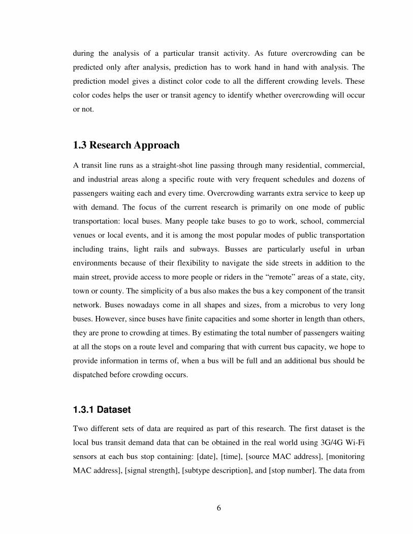
mobile application on smartphones or agency website. The colors in Figure 1-1 indicate
the entire demand on a route compared to the current load capacity of the public transit at
a given time.
8
Figure 1-1: Transit demand compared to load capacity
Green means the bus can accommodate all the passengers currently waiting at each stop
on the route without reaching capacity. The more red the road becomes, the more
crowded the bus will be. Gray indicates there is no available data.
1.4 Thesis Organization
This section describes the contents of each chapter. The thesis consists of 7 chapters
including the introductory chapter.
In Chapter 2, we review existing literature on some of the major applications and data
collection schemes in public transportation, followed by an overview of prediction and
simulation models.

9
In Chapter 3, we focus our discussion on the crowding prediction model, providing a
detailed definition of the crowding problem, alongside revealing crowding levels and
pushing analysis information to passengers.
In Chapter 4, we provide an overview of the system architecture.
In Chapter 5, we dive into the prototype implementation of the frontend and backend
functions. We describe the structure of the data collected from the bus and bus stop.
Also, we describe an approach for solving transit crowding.
In Chapter 6, we discuss the benefits and drawbacks of using our approach.
In Chapter 7, we conclude by reiterating the key points of the research and discussing
threats to the validity of our results as well as ideas for extending the research in the
future.
10
Chapter 2
2. LITERATURE REVIEW
2.1 Introduction
Transit demand estimation and crowding level predictions have gained attention because
of the increasing demand to capture high-quality, real-time data to enable intelligent
transit systems in order to meet the need by transit agencies to improve quality of transit
services and support transit operations and management. Data collected can include data
on the location of multi-modal public transit vehicles (buses, trams, rails, ferries, etc.)
from GPS and embedded systems and data from infrastructure and smartphones of riders
– known as crowd sourced data.
The Advanced Traveler Information System (ATIS) is one of the core components of the
Intelligent Transport System (ITS). ATIS is a means of gathering static and real-time
data, analyzing and distributing real-time information to the public or private. The system
depends on modern technologies, mainly wireless, to capture data. Transit data can be
captured using an array of sensors. Information can be distributed to users through the
web, smartphones and tablets. The information provided can be of great benefit such as to
provide increased safety, management of capacity, etc. [14]. Data can be historical or
real-time. Historical data is captured in previous time periods. Real-time data contains the
most up-to-date data. Based on captured data, prediction information can be made. There
are essentially two types of prediction information – namely long term and short term.
The long-term prediction information is used for transit planning and is suitable for use in
determining future supply and demand of transit conditions. The short-term prediction
11
information is suitable for transit management and is applicable to activities within a time
frame of some seconds to few hours. Short-term predictions of transit conditions are
needed for transit management and traveler information systems.
2.2 Data Collection Techniques
One of the early works on automated transit data collection is the estimation of passenger
loads, passenger miles and origin-destination patterns using location-stamped farebox
transactional data. “Transactional data” means a record is kept of each farebox
transaction – essentially each boarding. “Location-stamped” means the records contain
the location where the boarding occurs; the most recent stop at which the door is opened.
In order to measure passenger loads, passenger miles and origin-destination patterns;
records of passenger boardings as well as passenger alightings by each bus stop are very
important. Providing a location-stamp requires an automatic vehicle location (AVL)
system and its integration with the electronic farebox. According to Navick and Furth in
[15], for both effective transit planning and operation, transit agencies need not just data
on how many passengers they are carrying, but on where the passengers boarded and
alighted. This data is used to estimate system-wide passenger miles and a measure of
system use.
TravLink clearly showed the potential advantages of using automatic vehicle location
(AVL) at an early stage. It provided location information to riders before they board by
capturing data and transferring the data using AVL transmitters to an online service for
processing [16].
Seattle Wide-Area Information For Travelers (SWIFT) project included a Global
Positioning System (GPS) that determined location and provided direction for drivers
based on pre-selected destination [17].
Real time arrival information enhances the usability of the public transit [18]. In [19],
“information technology also provides the single greatest opportunity to enhance the
quality of the travel experience”. Trip planning tool such as Google Transit
12
(http://www.google.com/transit), integrates automatic vehicle location and automatic
passenger count data as well as station, stop, route, and schedule information from transit
agencies to transit users. Providing transit traveler information improves the customer
transit experience and the quality of service. While the trip planning tool can predict
vehicle arrival times based on real-time GPS data, it does not support the estimation of
total demand by passengers on a specific route and crowding level predictions at a given
time.
2.3 Prediction Models
A sound prediction model can be used to precisely forecast traffic and transit conditions
as well as transportation elements in real-time. Much research has been focused on
prediction models for public transit and traffic systems based on historical and/or real-
time data.
A large number of the prediction models are based on historical data. These include
regression and historical average techniques [20-22], machine learning [23], neural
networks [24-26], autoregressive integrated moving average (ARIMA) [27-29], and
fuzzy logic [30-31]. These methods can be subjected to complexity in computation. This
could be due to the static requirements or sizable number of estimated parameters and
may not be flexible to change in transportation patterns [32].
Smith et al. [33] carried out comparisons of time series, neural network, historical
average, and regression, and discovered that the non-parametric regression model notably
performed better than the other models. However, non-parametric regression models
involve a training process and sizable amount of historical data. If the matches are not
good enough in the historical data store, the regression may not provide a reliable
prediction. Therefore to make prediction accuracy better, different models were proposed
based on real-time traffic data [34-35].
A varying degree of accuracy has been achieved by these prediction models for
predicting arrival time, traffic state estimation, travel time, etc. However, some of the
13
models are based on traffic theory that is originally established for traffic systems and
does not necessarily hold for transit systems. In our work, we adopt a modeling approach
similar to Google traffic to develop a transit prediction model to facilitate estimation of
crowding levels.
According to [36] Google Maps displays real-time traffic information across many
countries. One of the layers on Google Maps illustrates colors of the roads in green,
yellow, red, or gray. The colors represent how fast the traffic is moving as follows:
• Green: more than 50 mi/h
• Yellow: 25 – 50 mi/h
• Red: less than 25 mi/h
• Gray: no data available
The traffic availability data that are provided for the roads are aggregated from several
sources including road sensors and cell phone users as traffic volunteers. Providing this
information helps Google traffic users to avoid congested roads.
2.4 Simulation Models
Simulation is one of the best tools to reproduce transportation information, if there are no
adequate transportation measurements available for estimation and prediction.
Transportation data can be measured using different types of equipment but it is very
costly to install, test and maintain a large-scale system. For experimental purposes or
proof of concept, a simulation model [37] can be used to simulate large metropolitan
areas with many travelers.
Simulation models can be macroscopic or microscopic. In freeway traffic, microscopic
models can represent individual vehicle movements. Macroscopic models represent
traffic flow in terms of aggregate measures such as density, flow rate, and space mean
14
speed. A microscopic model requires more computing time and resources. It can typify
vehicles in a more pragmatic manner than the macroscopic models. Microscopic models
theoretically are more reactive to dissimilar traffic strategies and can also produce more
accurate measure of effectiveness and give adequate flexibility to test myriad
combinations of supply and demand [38].
2.4 Summary
The basic model for predicting when the bus will be full is decided based on the literature
review. A new approach to predict ahead of time when a bus will be full is proposed
based on real-time data. This is done by estimating the total number of passengers present
at the bus stops on a specific route using Wi-Fi sensors and determining the total number
of passengers on a bus for the route using on-board sensors. Since the real-world data
may be unavailable, a simulated dataset is proposed to emulate transit operations. We
will combine this data and apply the prediction model to estimate crowding level
conditions at a given time for the route.
15
Chapter 3
3. THE PROPOSED CROWDING PREDICTION MODEL
3.1 Problem definition
Crowding is calculated on a route basis. This means that for a given route between the
origin and destination, the entire demand and the entire capacity over that route is used to
determine the level of crowding over the route. For each route, there is an origin-
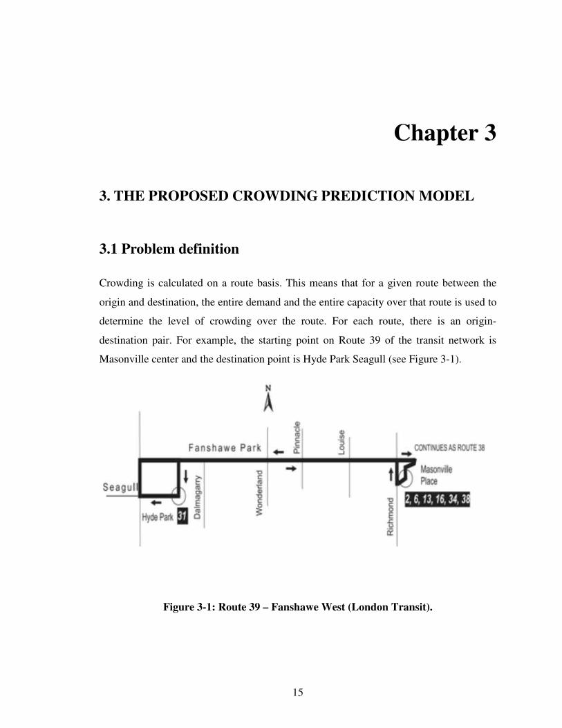
destination pair. For example, the starting point on Route 39 of the transit network is
Masonville center and the destination point is Hyde Park Seagull (see Figure 3-1).
Figure 3-1: Route 39 – Fanshawe West (London Transit).
16
The goal of our problem are to determine the number of passengers on a bus and estimate
the demand on a route in urban transit network based on real-time transit information and
predict or estimate the crowding level at a given time before crowding occurs.
We assume in an urban network there is a centralized transit operation center that
periodically determines transit activity and generates crowding predictions. The
operation center considers the transit network as a discrete-time system to conduct the
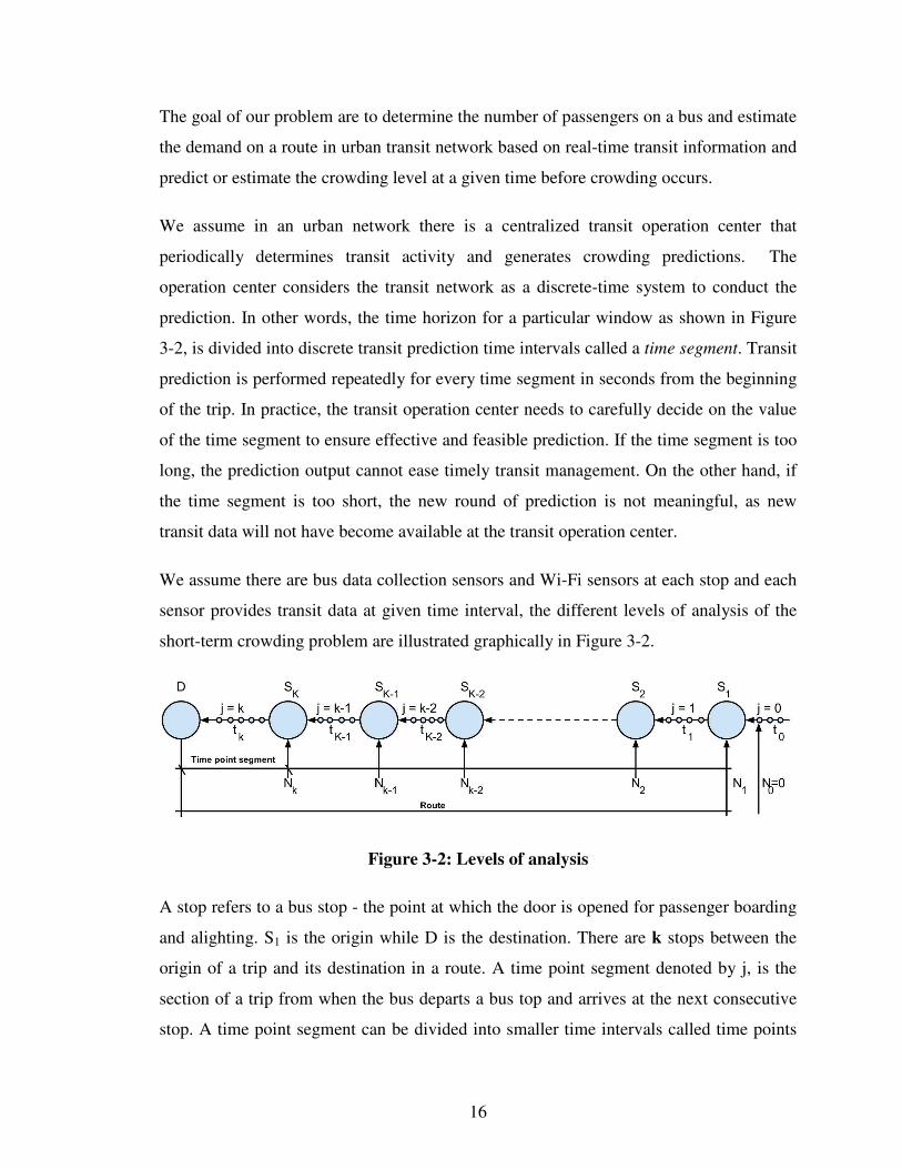
prediction. In other words, the time horizon for a particular window as shown in Figure
3-2, is divided into discrete transit prediction time intervals called a time segment. Transit
prediction is performed repeatedly for every time segment in seconds from the beginning
of the trip. In practice, the transit operation center needs to carefully decide on the value
of the time segment to ensure effective and feasible prediction. If the time segment is too
long, the prediction output cannot ease timely transit management. On the other hand, if
the time segment is too short, the new round of prediction is not meaningful, as new
transit data will not have become available at the transit operation center.
We assume there are bus data collection sensors and Wi-Fi sensors at each stop and each
sensor provides transit data at given time interval, the different levels of analysis of the
short-term crowding problem are illustrated graphically in Figure 3-2.
Figure 3-2: Levels of analysis
A stop refers to a bus stop - the point at which the door is opened for passenger boarding
and alighting. S1 is the origin while D is the destination. There are k stops between the
origin of a trip and its destination in a route. A time point segment denoted by j, is the
section of a trip from when the bus departs a bus top and arrives at the next consecutive
stop. A time point segment can be divided into smaller time intervals called time points
17
denoted by t in the diagram. Bus data is measured at time points and passenger presence
is measured at the stops. Bus data collected within a time point segment is combined with
the total number of passengers waiting at the stops that are ahead of that particular time
point segment. NK refers to the number of passengers present at a stop. N0 , with value
taken to be zero, is the number of passengers before the origin of the trip.
3.2 Applying prediction model to TraDEPS
We apply the proposed transit crowding prediction model to a typical centralized Transit
Demand Estimation and Prediction System (TraDEPS) to construct a proactive TraDEPS.
The proposed TraDEPS operates in two phases: (1) revealing and crowding level
prediction, and (2) pushing analysis information to passengers. Each of the phases is
described in detail below:
3.2.1 Revealing and crowding level prediction
TraDEPS periodically collects transit data, e.g. the number of passengers on the bus and
the entire number of passengers waiting at all the stops ahead of the current time point
segment at a time t. Based on the real-time data collected, the service predicts for a route
using the prediction model, and then reveals transit crowding level using the equations in
Table 3-1. A bus will be crowded if Equation 1 is satisfied
(1)
Here L is the current number of passengers on a bus, C is the capacity of the bus, j is the
current time point segment during which crowding level is measured. k is the number of
bus stops on the route. is the consecutive stop after the current time point
segment, j.
Based on this condition, the agency can react in real time to the shift in transit amount by
dispatching an additional bus.
18
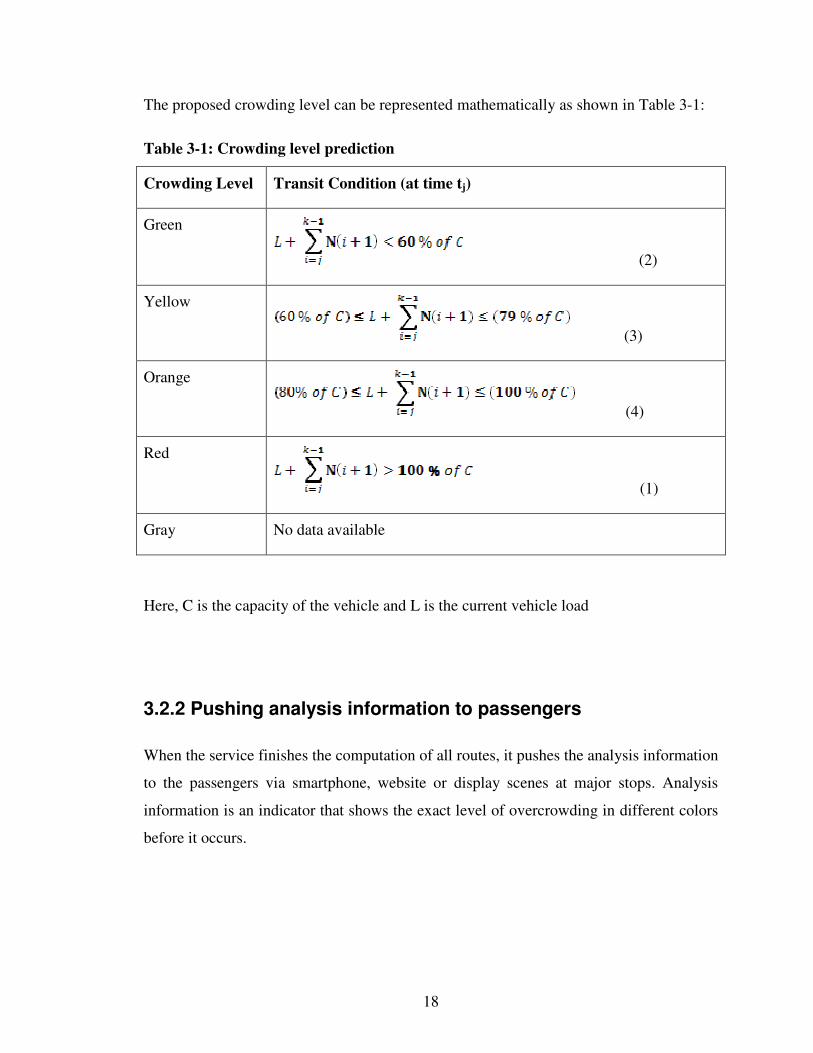
The proposed crowding level can be represented mathematically as shown in Table 3-1:
Table 3-1: Crowding level prediction
Crowding Level Transit Condition (at time tj)
Green
(2)
Yellow
(3)
Orange
(4)
Red
(1)
Gray No data available
Here, C is the capacity of the vehicle and L is the current vehicle load
3.2.2 Pushing analysis information to passengers
When the service finishes the computation of all routes, it pushes the analysis information
to the passengers via smartphone, website or display scenes at major stops. Analysis
information is an indicator that shows the exact level of overcrowding in different colors
before it occurs.

19
Chapter 4
4. SYSTEM DESIGN
4.1 System Architecture
This section provides an overview of the Transit Demand Estimation and Prediction
System (TraDEPS). The architecture is divided into front end to collect data and backend
services for data analytics and prediction. The high-level system architecture is presented
as shown in Figure 4-1:
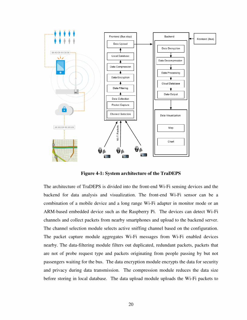
20
Figure 4-1: System architecture of the TraDEPS
The architecture of TraDEPS is divided into the front-end Wi-Fi sensing devices and the
backend for data analysis and visualization. The front-end Wi-Fi sensor can be a
combination of a mobile device and a long range Wi-Fi adapter in monitor mode or an
ARM-based embedded device such as the Raspberry Pi. The devices can detect Wi-Fi
channels and collect packets from nearby smartphones and upload to the backend server.
The channel selection module selects active sniffing channel based on the configuration.
The packet capture module aggregates Wi-Fi messages from Wi-Fi enabled devices
nearby. The data-filtering module filters out duplicated, redundant packets, packets that
are not of probe request type and packets originating from people passing by but not
passengers waiting for the bus. The data encryption module encrypts the data for security
and privacy during data transmission. The compression module reduces the data size
before storing in local database. The data upload module uploads the Wi-Fi packets to
21
the backend server. We combine the data that is collected from the front-end bus sensor
with the data from the bus stops.
The backend consists of a data analysis service running on the server. It provides data
decryption and decompression for the filtered, encrypted and compressed messages
received from the front-end devices. The data processing module processes the captured
data using data analysis techniques and stores the results in the backend database. The
data output module updates the data visualization module with relevant analysis results.
A data visualization module can be a web or mobile interface for viewing analyzed
information received from the data output module in real-time in form of charts and
maps.
4.2 Data Collection
The data collection module consists of the IEEE 802.11 packet capture and channel
selection modules. The channel selection module is used to select a channel. Wi-Fi
sensors installed at each stop can be used to detect probe requests sent by WiFi enabled
devices. WiFi devices including smartphones such as iPhone, Android, broadcast
messages at certain intervals depending on the state of the device (see Table 4-1). Mobile
devices send probe requests for network information from nearby access points or nodes.
These devices need not be connected to the access points for their presence to be
detected.
The data needed for the analytics include data from each bus as well as aggregated
presence data from bus stops for a specific route. The data from the bus include detailed
information about the load of passengers, arrival time, longitude and latitude, route
number, direction of travel, and date. Usually GPS, IPS, automatic passenger counter
and other onboard embedded devices are used for data collection and transmission.
Regarding the transit data for the entire demand on each route, the date, time, MAC
addresses of smartphones, MAC address of Wi-Fi sensor, received signal strength
indication (rssi), subtype description, and stop number can be obtained from the Wi-Fi
22
sensors placed at each bus stop to detect smartphone devices. Smartphones send out
messages as they search for Wi-Fi networks nearby. These messages include the phone's
MAC address (a unique string of letters and numbers), signal strength, and other non-
personally identifiable information.
The main goal of detecting devices is to measure the number of people that are present at
each bus stop and compute the total number of riders waiting on a route level at a given
time allowing the study of evolution of crowding.
Table 4-1: Probe request interval for smartphone devices using various platforms
(iOS, Android and others) – influenced by the applications running on the device
and other factors.
Device State Probe Request Interval (Smartphones)
Asleep Approximately once a minute
Standby 9 – 16 times per minute
Connected Varies
Wi-Fi nodes can detect probe requests from Wi-Fi devices up to 20 metres and above and
upload the data to a server or cloud-based system.
4.2.1 Packet Capture
The Wi-Fi sensor in the front-end is an embedded device that can capture Wi-Fi
messages from Wi-Fi enabled devices in the neighborhood including probe requests from
smartphones before transfer to the server or backend cloud. The packet capture module
not only collects IEEE 802.11 frames or packet information, it also logs packet
information locally and for immediate transfers. The network interface must be in
monitor mode in order to capture all of the packets.
23
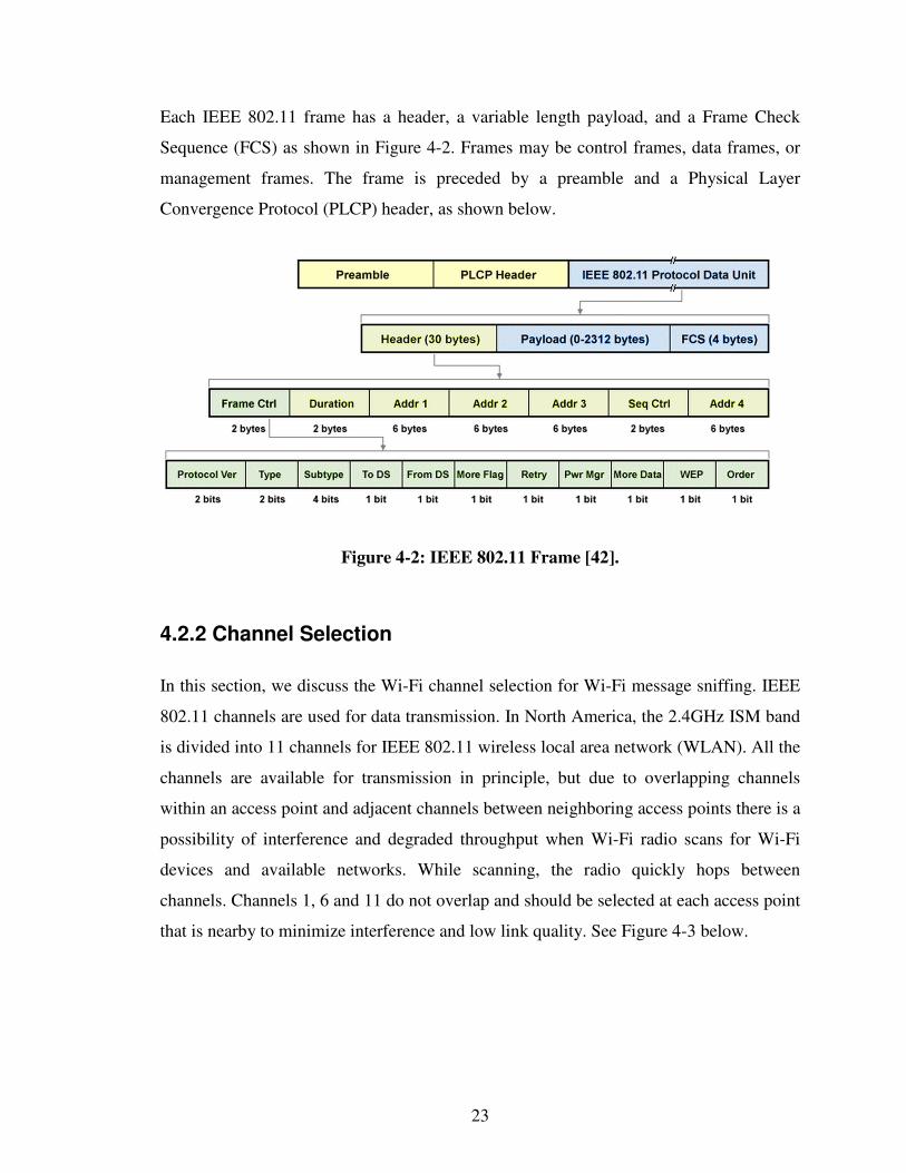
Each IEEE 802.11 frame has a header, a variable length payload, and a Frame Check
Sequence (FCS) as shown in Figure 4-2. Frames may be control frames, data frames, or
management frames. The frame is preceded by a preamble and a Physical Layer
Convergence Protocol (PLCP) header, as shown below.
Figure 4-2: IEEE 802.11 Frame [42].
4.2.2 Channel Selection
In this section, we discuss the Wi-Fi channel selection for Wi-Fi message sniffing. IEEE
802.11 channels are used for data transmission. In North America, the 2.4GHz ISM band
is divided into 11 channels for IEEE 802.11 wireless local area network (WLAN). All the
channels are available for transmission in principle, but due to overlapping channels
within an access point and adjacent channels between neighboring access points there is a
possibility of interference and degraded throughput when Wi-Fi radio scans for Wi-Fi
devices and available networks. While scanning, the radio quickly hops between
channels. Channels 1, 6 and 11 do not overlap and should be selected at each access point
that is nearby to minimize interference and low link quality. See Figure 4-3 below.
24
Figure 4-3: Wi-Fi channels in the 2.4 GHz band (Wikipedia).
Wi-Fi Channel selection monitors Wi-Fi signals and probe messages from Wi-Fi enabled
devices including probe requests from smartphones. Smartphones can transmit Wi-Fi
probe requests to all 11 channels and send Wi-Fi data messages in the fixed channel
associated with a Wi-Fi sensor in a connected Wi-Fi network. The channel selection
module chooses better active sniffing channels based on the configuration by a user.
4.3 Front-end Bus
Data is collected from the sensors on-board the buses and sent to the central server. The
agency collects the location of a vehicle and number of passengers that are boarding and
de-boarding.
4.4 Data Filtering
The filtering module is used to filter out packets that are not of probe request type and not
originating from smartphones as well as people that are just walking by the stop but not
real passengers. Once a Wi-Fi sensor has received data for period of time, computation
follows including the removal of unwanted data.
The filtering module logs only those captured packets that contain probe requests from
smartphone devices. All redundant, duplicated, or non-smartphone-device data packets
are discarded. The filtered packet information is logged for file transfer to the backend
server as an HTTP POST request. Filtering criteria are specified at runtime. As shown in
25
Table 4-2, all probe requests have a subtype value of “0100” in binary (4 in decimal) and
a type value of “00” in binary (0 in decimal). These values can be used to filter and
isolate all probe requests with 'wlan.fc.type == 0 && wlan.fc.subtype == 4'.
Table 4-2: Frame type and Subtype
26
There is also a need to separate the riders waiting for public transit at a bus stop from
pedestrians just passing by or outside the area. This can be determined from the signal
strength and the time spent at the location. The smartphone device sending the probe
requests can be classified into two different states – the passerby and the passenger state.
Any device seen by the Wi-Fi node is regarded as a passerby and device seen with high
signal strength for a certain time period is referred to as a passenger.
Figure 4-4: Computing passenger state
It is necessary to determine the people passing by the bus stop versus passengers actually
waiting at the stop. The devices in passerby and passenger state can represent people
passing by and the passengers waiting for bus respectively. The two different device
states are computed using a variety of techniques. A passerby is any device that was seen
at least once, while a passenger is any device seen for a certain time with high signal
strength. Timestamps of probe requests from devices are used to compute how long
someone was within the access point or Wi-Fi sensor range.
27
4.4.1 Multiple Devices
The Wi-Fi sensor cannot differentiate the type of device looking for a network. If a rider
is carrying a laptop, smartphone, portable media player, and a tablet, the system will
count them all. This will seriously affect the counting analytics and increase the numbers
of people counted. In a real-world implementation, Wi-Fi sensors will collect millions of
packets from thousands of different devices per day, week or month. The IEEE OUI
Registry [39] can filter out those devices that are not smartphones before data encryption
and transmission. ALGORITHM 1 shows a pseudo code to maintain a MAC library of
smartphone brands in the IEEE OUI registry and dictionary of collected Wi-Fi packets. It
eliminates packets that are not from smartphone devices based on the registry.
ALGORITHM 1: Data filtering using IEEE OUI registry
4.5 Data encryption and decryption
Transmitted data is susceptible to eavesdropping by unauthorized users. As a result,
transmitted data are subjected to encryption to ensure security and privacy of the data.
Encryption is the operation of converting unhidden or plain data into hidden or cryptic
data. This is done to make the data private for the recipient designated to receive it.
Encryption techniques are used to protect the data transferred via wireless sensors. Each
smartphone’s MAC address is also scrambled or anonymized with a one-way hash.
28
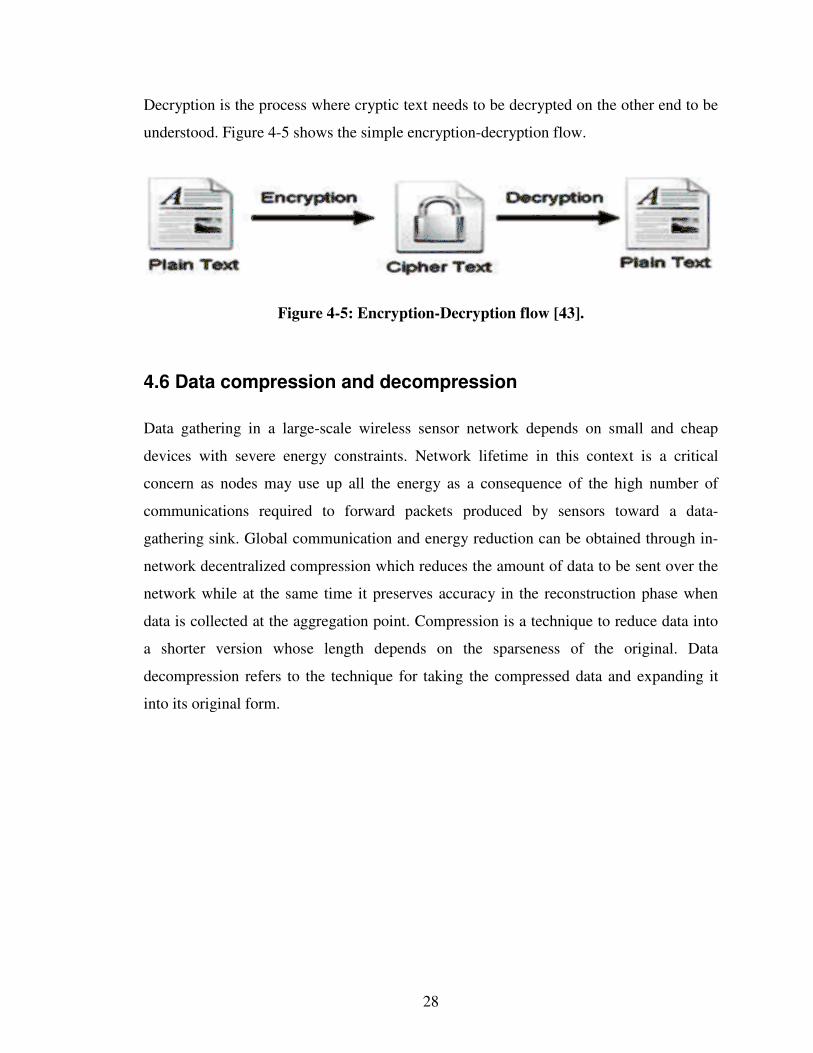
Decryption is the process where cryptic text needs to be decrypted on the other end to be
understood. Figure 4-5 shows the simple encryption-decryption flow.
Figure 4-5: Encryption-Decryption flow [43].
4.6 Data compression and decompression
Data gathering in a large-scale wireless sensor network depends on small and cheap
devices with severe energy constraints. Network lifetime in this context is a critical
concern as nodes may use up all the energy as a consequence of the high number of
communications required to forward packets produced by sensors toward a data-
gathering sink. Global communication and energy reduction can be obtained through in-
network decentralized compression which reduces the amount of data to be sent over the
network while at the same time it preserves accuracy in the reconstruction phase when
data is collected at the aggregation point. Compression is a technique to reduce data into
a shorter version whose length depends on the sparseness of the original. Data
decompression refers to the technique for taking the compressed data and expanding it
into its original form.
29
4.7 Data processing, local and cloud databases
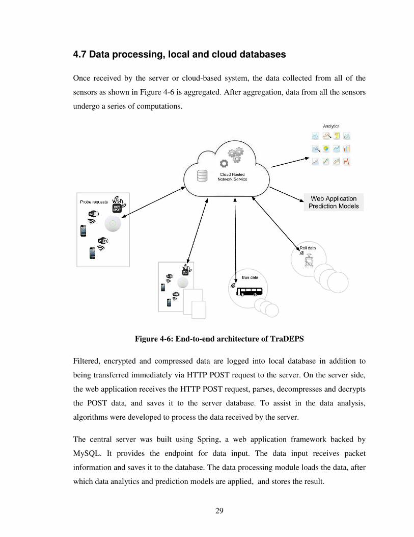
Once received by the server or cloud-based system, the data collected from all of the
sensors as shown in Figure 4-6 is aggregated. After aggregation, data from all the sensors
undergo a series of computations.
Figure 4-6: End-to-end architecture of TraDEPS
Filtered, encrypted and compressed data are logged into local database in addition to
being transferred immediately via HTTP POST request to the server. On the server side,
the web application receives the HTTP POST request, parses, decompresses and decrypts
the POST data, and saves it to the server database. To assist in the data analysis,
algorithms were developed to process the data received by the server.
The central server was built using Spring, a web application framework backed by
MySQL. It provides the endpoint for data input. The data input receives packet
information and saves it to the database. The data processing module loads the data, after
which data analytics and prediction models are applied, and stores the result.
30
4.8 Data output and Visualization
The data output module updates the data visualization module with relevant analysis
results. The analysis results received from the data output module is displayed as
crowding level on the server. The server presents the web interface to view the
information in the form of charts and maps.
4.10 TraDEPS and Privacy
The collection of location data and MAC addresses can be a concern to the riders.
Therefore the issue of privacy is addressed in the TraDEPS. MAC addresses are usually
processed and anonymized using a hash function by making it impossible to recover the
original MAC address from the processed MAC address. At the end of each day, location
data and other private information are deleted from the data store.
4.11 Summary
The Transit Demand Estimation and Prediction System architecture is a centralized
system for real-time data collection and analysis. We apply the proposed transit crowding
prediction model to the centralized TraDEPS to construct a proactive TraDEPS. The
proactive TraDEPS is of benefit in revealing and making crowding level prediction, as
well as pushing analysis information to passengers.
31
Chapter 5
5 PROTOTYPE IMPLEMENTATION
5.1 Prototype Implementation of Frontend Functions
In this research, we designed and implemented the front-end modules of TraDEPS for
collecting data at the bus stops. The Wi-Fi sensor used to determine passenger presence
at the stop consists of several modules providing functions ranging from data collection,
including packet capture and data filtering, to data offload to the backend server. We
explored two different front-end methods.
(1) The first method involved the use of Raspberry Pi; model B [32] with TP-LINK TL-
WN722N USB Wi-Fi adapter. The Raspberry Pi Model B is a very small computer with
512MB of RAM, two usb ports, an SD card slot and runs Linux. It is based on the ARM
11 CPU 700MHz. An 8 GB SD card was used to store the operating system and software.
The TP-LINK TL-WN722N USB Wi-Fi adapter was connected to the Raspberry Pi. The
adapter supports monitor mode, “b”, “a”, “g”, and “n” type networks and comes with a
high-gain antenna. A USB micro power supply is connected to the Pi to provide power to
the Wi-Fi adapter and the Pi. An Ethernet cable was used to connect the Pi to the Internet
and the local network. Probe requests captured by the Wi-Fi adapter are collected and
transmitted to the server through the Ethernet cable. Figure 5-1 depicts the screen-shot of
a Wi-Fi node based on the raspberry pi model B.
The software installed on the SD card includes Python, Linux and Tshark. Wireshark is a
network protocol analyzer [40]. It allows the capture of packet data and filtering of data
transmitted across a live network or the reading of packet data from a previously saved
capture file. While Wireshark provides a GUI interface for data capture and filtering
tasks, Tshark is the command-line equivalent of Wireshark. It is a perfect fit for the low-
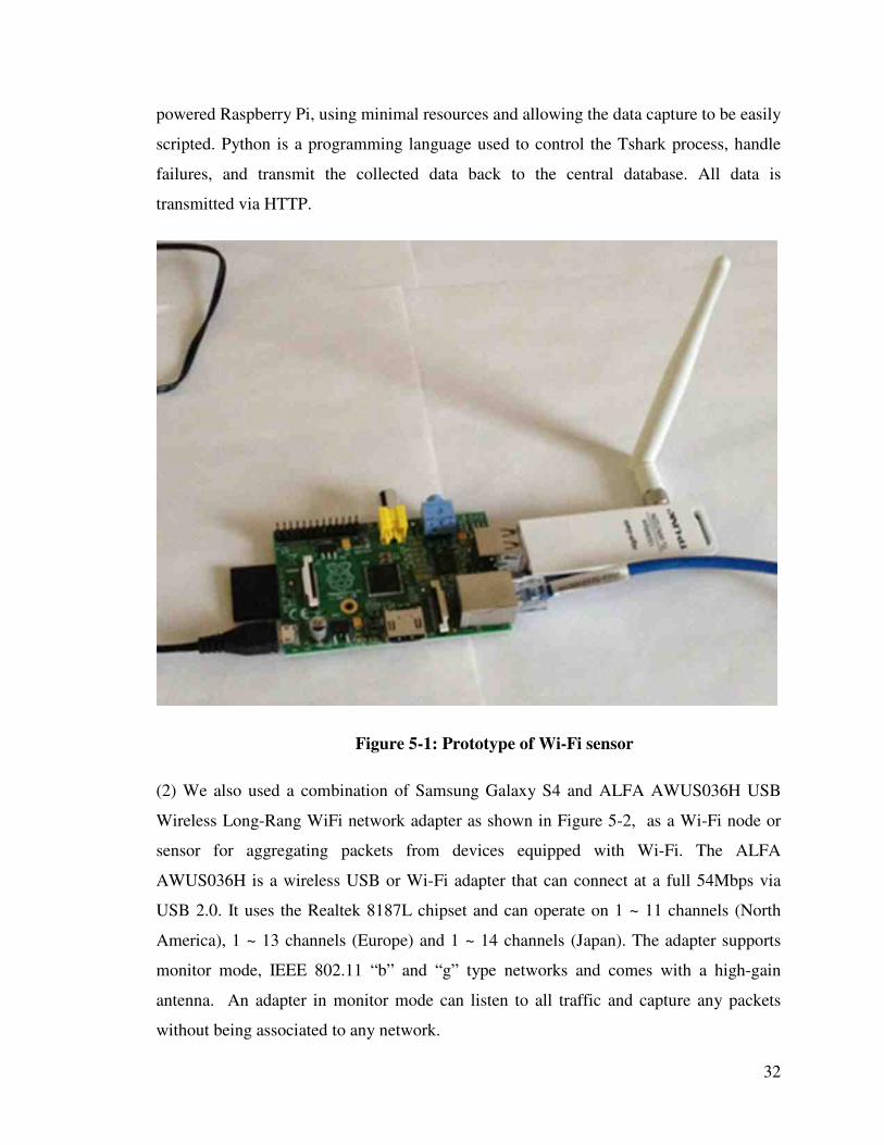
32
powered Raspberry Pi, using minimal resources and allowing the data capture to be easily
scripted. Python is a programming language used to control the Tshark process, handle
failures, and transmit the collected data back to the central database. All data is
transmitted via HTTP.
Figure 5-1: Prototype of Wi-Fi sensor
(2) We also used a combination of Samsung Galaxy S4 and ALFA AWUS036H USB
Wireless Long-Rang WiFi network adapter as shown in Figure 5-2, as a Wi-Fi node or
sensor for aggregating packets from devices equipped with Wi-Fi. The ALFA
AWUS036H is a wireless USB or Wi-Fi adapter that can connect at a full 54Mbps via
USB 2.0. It uses the Realtek 8187L chipset and can operate on 1 ~ 11 channels (North
America), 1 ~ 13 channels (Europe) and 1 ~ 14 channels (Japan). The adapter supports
monitor mode, IEEE 802.11 “b” and “g” type networks and comes with a high-gain
antenna. An adapter in monitor mode can listen to all traffic and capture any packets
without being associated to any network.
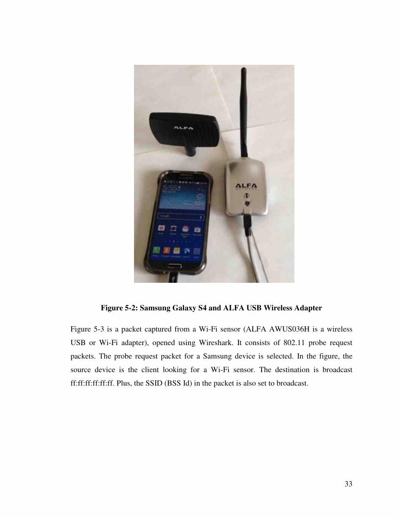
33
Figure 5-2: Samsung Galaxy S4 and ALFA USB Wireless Adapter
Figure 5-3 is a packet captured from a Wi-Fi sensor (ALFA AWUS036H is a wireless
USB or Wi-Fi adapter), opened using Wireshark. It consists of 802.11 probe request
packets. The probe request packet for a Samsung device is selected. In the figure, the
source device is the client looking for a Wi-Fi sensor. The destination is broadcast
ff:ff:ff:ff:ff:ff. Plus, the SSID (BSS Id) in the packet is also set to broadcast.
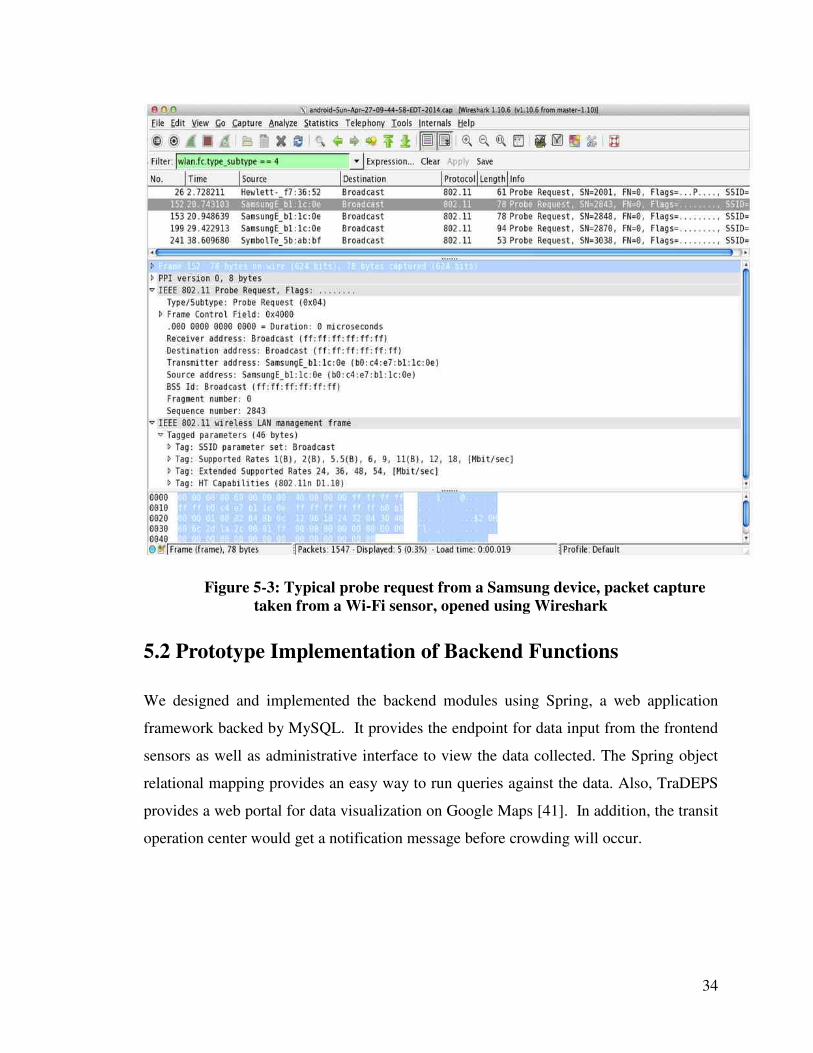
34
Figure 5-3: Typical probe request from a Samsung device, packet capture
taken from a Wi-Fi sensor, opened using Wireshark
5.2 Prototype Implementation of Backend Functions
We designed and implemented the backend modules using Spring, a web application
framework backed by MySQL. It provides the endpoint for data input from the frontend
sensors as well as administrative interface to view the data collected. The Spring object
relational mapping provides an easy way to run queries against the data. Also, TraDEPS
provides a web portal for data visualization on Google Maps [41]. In addition, the transit
operation center would get a notification message before crowding will occur.
35
5.3 Creating a Simulated Dataset
This section deals with creating new datasets. The infrastructure for collecting transit data
for this research is not in place; wireless access points at each bus stop would be required.
While this is not particularly costly, it was beyond the scope of the research, let alone to
acquire permission from the local transit authority to install access point. In practice,
data collection is distributed. The hardware used for our experiment cannot be used for
data collection for all bus stops and buses in different locations, but we can use it to
collect real data in a location. As a result, simulation data is the best way to produce
transit information, when there are no adequate transit measurements available.
Wi-Fi enabled devices send probe requests periodically depending on the vendor. Probe
requests can be typically sent between 15 seconds and 1 minute. Sniffing probe requests
using hardware is an easy task since they are sent in the clear over all channels of
transmission in sequence.
Table 5-1 below shows an example of probe requests sent by devices with MAC
addresses 04:f0:21:09:86:d1 and 98:03:d8:7f:3c:9f.
Table 5-1: Example of real data monitored by a Wi-Fi sensor at a bus stop
Frame
Control
Destination
address
Source
address
BSS Id RSSI Frame
Number
Arrival Time
0x4000 ff:ff:ff:ff:ff:ff 04:f0:21:09:86:d1 ff:ff:ff:ff:ff:ff -30 103 Aug 8, 2014
13:31:30.628808000
EDT
0x4000 ff:ff:ff:ff:ff:ff 98:03:d8:7f:3c:9f ff:ff:ff:ff:ff:ff -32 137 Aug 8, 2014
13:31:34.065392000
EDT
The data transmitted through the WiFi sensor to the backend and stored in the database
include:
• Date: when the packet is captured.
36
• Time: when the packet is captured.
• Mac address of the WiFi sensor or access point.
• MAC address: the mac address of the smartphone from which packets emanated.
• Received signal strength (in dBm) from the smartphone device.
• Stop Number: the stop corresponding to the WiFi sensor
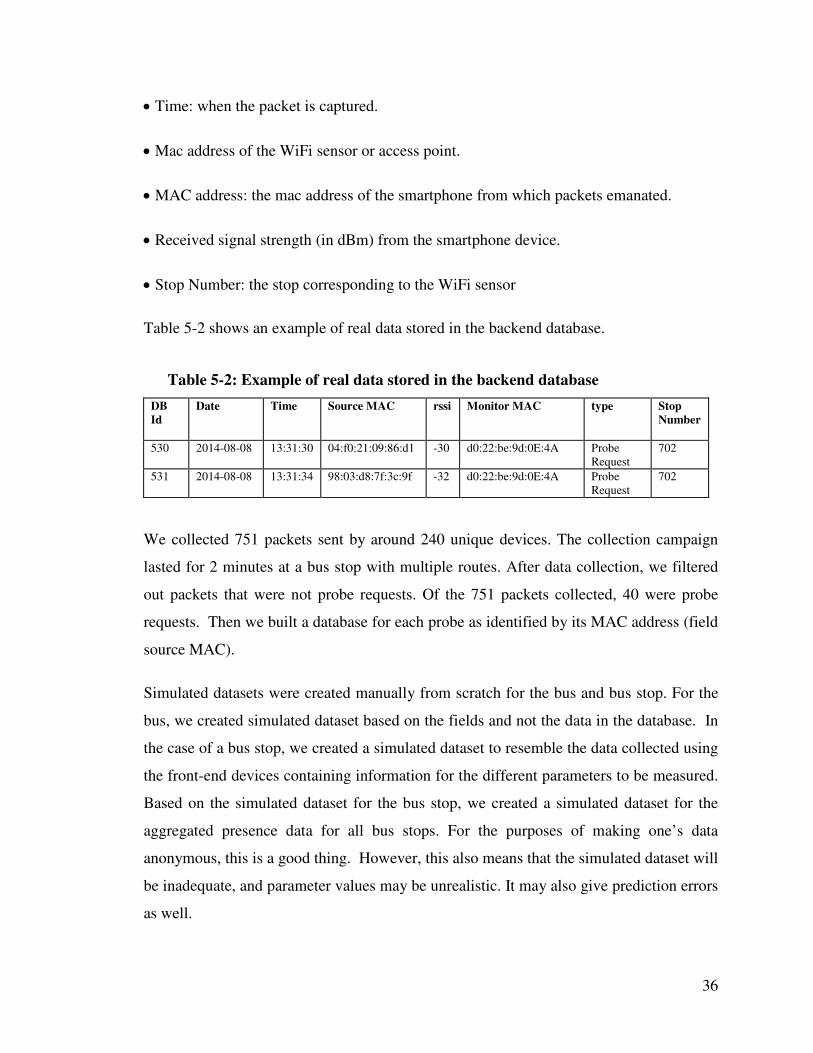
Table 5-2 shows an example of real data stored in the backend database.
Table 5-2: Example of real data stored in the backend database
DB
Id
Date Time Source MAC rssi Monitor MAC type Stop
Number
530 2014-08-08 13:31:30 04:f0:21:09:86:d1 -30 d0:22:be:9d:0E:4A Probe
Request
702
531 2014-08-08 13:31:34 98:03:d8:7f:3c:9f -32 d0:22:be:9d:0E:4A Probe
Request
702
We collected 751 packets sent by around 240 unique devices. The collection campaign
lasted for 2 minutes at a bus stop with multiple routes. After data collection, we filtered
out packets that were not probe requests. Of the 751 packets collected, 40 were probe
requests. Then we built a database for each probe as identified by its MAC address (field
source MAC).
Simulated datasets were created manually from scratch for the bus and bus stop. For the
bus, we created simulated dataset based on the fields and not the data in the database. In
the case of a bus stop, we created a simulated dataset to resemble the data collected using
the front-end devices containing information for the different parameters to be measured.
Based on the simulated dataset for the bus stop, we created a simulated dataset for the
aggregated presence data for all bus stops. For the purposes of making one’s data
anonymous, this is a good thing. However, this also means that the simulated dataset will
be inadequate, and parameter values may be unrealistic. It may also give prediction errors
as well.
37
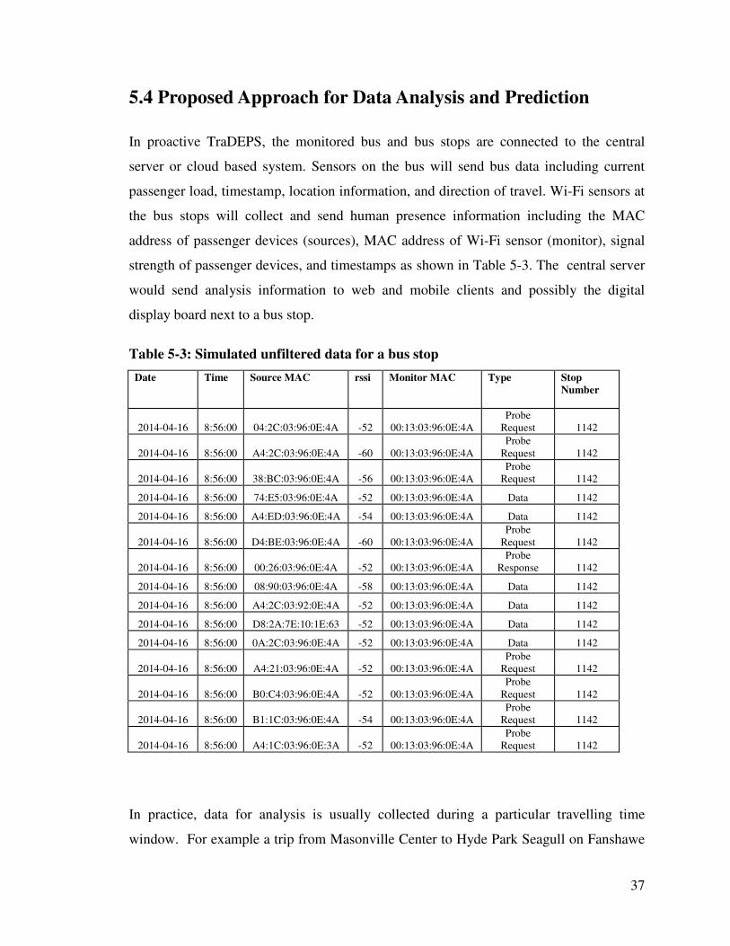
5.4 Proposed Approach for Data Analysis and Prediction
In proactive TraDEPS, the monitored bus and bus stops are connected to the central
server or cloud based system. Sensors on the bus will send bus data including current
passenger load, timestamp, location information, and direction of travel. Wi-Fi sensors at
the bus stops will collect and send human presence information including the MAC
address of passenger devices (sources), MAC address of Wi-Fi sensor (monitor), signal
strength of passenger devices, and timestamps as shown in Table 5-3. The central server
would send analysis information to web and mobile clients and possibly the digital
display board next to a bus stop.
Table 5-3: Simulated unfiltered data for a bus stop
Date Time Source MAC rssi Monitor MAC Type Stop
Number
2014-04-16 8:56:00 04:2C:03:96:0E:4A -52 00:13:03:96:0E:4A
Probe
Request 1142
2014-04-16 8:56:00 A4:2C:03:96:0E:4A -60 00:13:03:96:0E:4A
Probe
Request 1142
2014-04-16 8:56:00 38:BC:03:96:0E:4A -56 00:13:03:96:0E:4A
Probe
Request 1142
2014-04-16 8:56:00 74:E5:03:96:0E:4A -52 00:13:03:96:0E:4A Data 1142
2014-04-16 8:56:00 A4:ED:03:96:0E:4A -54 00:13:03:96:0E:4A Data 1142
2014-04-16 8:56:00 D4:BE:03:96:0E:4A -60 00:13:03:96:0E:4A
Probe
Request 1142
2014-04-16 8:56:00 00:26:03:96:0E:4A -52 00:13:03:96:0E:4A
Probe
Response 1142
2014-04-16 8:56:00 08:90:03:96:0E:4A -58 00:13:03:96:0E:4A Data 1142
2014-04-16 8:56:00 A4:2C:03:92:0E:4A -52 00:13:03:96:0E:4A Data 1142
2014-04-16 8:56:00 D8:2A:7E:10:1E:63 -52 00:13:03:96:0E:4A Data 1142
2014-04-16 8:56:00 0A:2C:03:96:0E:4A -52 00:13:03:96:0E:4A Data 1142
2014-04-16 8:56:00 A4:21:03:96:0E:4A -52 00:13:03:96:0E:4A
Probe
Request 1142
2014-04-16 8:56:00 B0:C4:03:96:0E:4A -52 00:13:03:96:0E:4A
Probe
Request 1142
2014-04-16 8:56:00 B1:1C:03:96:0E:4A -54 00:13:03:96:0E:4A
Probe
Request 1142
2014-04-16 8:56:00 A4:1C:03:96:0E:3A -52 00:13:03:96:0E:4A
Probe
Request 1142
In practice, data for analysis is usually collected during a particular travelling time
window. For example a trip from Masonville Center to Hyde Park Seagull on Fanshawe
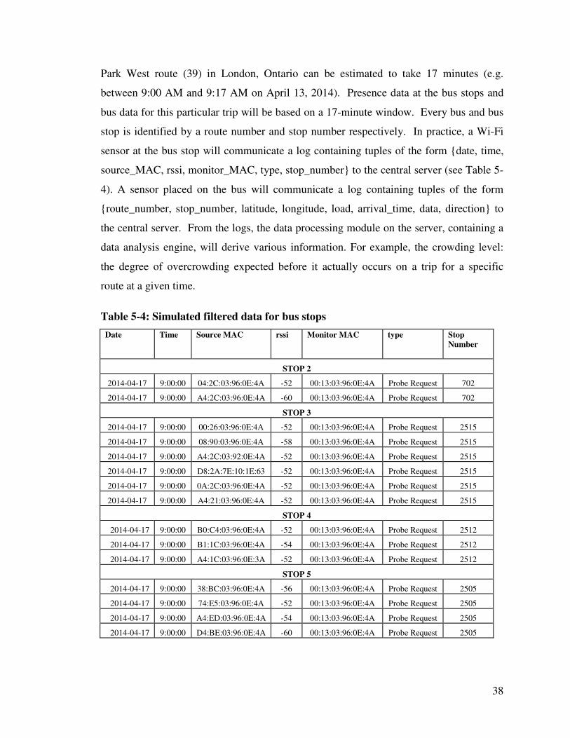
38
Park West route (39) in London, Ontario can be estimated to take 17 minutes (e.g.
between 9:00 AM and 9:17 AM on April 13, 2014). Presence data at the bus stops and
bus data for this particular trip will be based on a 17-minute window. Every bus and bus
stop is identified by a route number and stop number respectively. In practice, a Wi-Fi
sensor at the bus stop will communicate a log containing tuples of the form {date, time,
source_MAC, rssi, monitor_MAC, type, stop_number} to the central server (see Table 5-
4). A sensor placed on the bus will communicate a log containing tuples of the form
{route_number, stop_number, latitude, longitude, load, arrival_time, data, direction} to
the central server. From the logs, the data processing module on the server, containing a
data analysis engine, will derive various information. For example, the crowding level:
the degree of overcrowding expected before it actually occurs on a trip for a specific
route at a given time.
Table 5-4: Simulated filtered data for bus stops
Date Time Source MAC rssi Monitor MAC type Stop
Number
STOP 2
2014-04-17 9:00:00 04:2C:03:96:0E:4A -52 00:13:03:96:0E:4A Probe Request 702
2014-04-17 9:00:00 A4:2C:03:96:0E:4A -60 00:13:03:96:0E:4A Probe Request 702
STOP 3
2014-04-17 9:00:00 00:26:03:96:0E:4A -52 00:13:03:96:0E:4A Probe Request 2515
2014-04-17 9:00:00 08:90:03:96:0E:4A -58 00:13:03:96:0E:4A Probe Request 2515
2014-04-17 9:00:00 A4:2C:03:92:0E:4A -52 00:13:03:96:0E:4A Probe Request 2515
2014-04-17 9:00:00 D8:2A:7E:10:1E:63 -52 00:13:03:96:0E:4A Probe Request 2515
2014-04-17 9:00:00 0A:2C:03:96:0E:4A -52 00:13:03:96:0E:4A Probe Request 2515
2014-04-17 9:00:00 A4:21:03:96:0E:4A -52 00:13:03:96:0E:4A Probe Request 2515
STOP 4
2014-04-17 9:00:00 B0:C4:03:96:0E:4A -52 00:13:03:96:0E:4A Probe Request 2512
2014-04-17 9:00:00 B1:1C:03:96:0E:4A -54 00:13:03:96:0E:4A Probe Request 2512
2014-04-17 9:00:00 A4:1C:03:96:0E:3A -52 00:13:03:96:0E:4A Probe Request 2512
STOP 5
2014-04-17 9:00:00 38:BC:03:96:0E:4A -56 00:13:03:96:0E:4A Probe Request 2505
2014-04-17 9:00:00 74:E5:03:96:0E:4A -52 00:13:03:96:0E:4A Probe Request 2505
2014-04-17 9:00:00 A4:ED:03:96:0E:4A -54 00:13:03:96:0E:4A Probe Request 2505
2014-04-17 9:00:00 D4:BE:03:96:0E:4A -60 00:13:03:96:0E:4A Probe Request 2505
39
We next show an operation analysis as example of the kinds of analyses that can be
performed by using the simulated datasets in the absence of real monitoring logs. For
constructing the simulated datasets, we manually created excel dataset files from scratch.
Our simulation consists of ten bus stops namely: S1, S2, S3, S4, S5, S6, S7, S8, S9 and
S10 with the corresponding number of passengers waiting at each bus top denoted by N1,
N2, N3, N4, N5, N6, N7, N8, N9 and N10 respectively. Furthermore, the simulation
consists of one bus running on one route namely Route 39: S1->S2->S3->S4->S5->S6-
>S7->S8->S9->S10. In the case of the simulated filtered dataset for the bus data, we
randomly inserted sets of values corresponding to each parameter in the tuples of the
form {route_number, stop_number, latitude, longitude, load, arrival_time, data,
direction} as shown in Table 5-5.
Table 5-5: Simulated data for a bus
Route
number
Stop
number Latitude Longitude Load
Arrival
time Date Direction
39 1142 43.0254714 81.2816004 8 9:00:00 2014-04-17 4
39 NA 43.0250824 81.2855363 8 9:01:35 2014-04-17 4
39 702 43.0246933 81.2894723 10 9:02:00 2014-04-17 4
39 NA 43.024436 -81.290366 10 9:02:08 2014-04-17 4
39 NA 43.02395 -81.291932 10 9:02:15 2014-04-17 4
39 2512 43.0231075 81.2948788 12 9:02:30 2014-04-17 4
39 NA 43.023793 -81.295469 12 9:02:50 2014-04-17 4
39 2515 43.0215725 81.3001718 20 9:03:00 2014-04-17 4
39 NA 43.02167 -81.304638 20 9:03:40 2014-04-17 4
39 NA 43.020011 -81.305228 20 9:04:10 2014-04-17 4
39 2505 43.0198313 81.3061591 28 9:05:00 2014-04-17 4
39 NA 43.019467 -81.307162 28 9:05:24 2014-04-17 4
39 2517 43.0189003 81.3094726 38 9:06:12 2014-04-17 4
39 NA 43.018197 -81.311797 38 9:07:04 2014-04-17 4
39 NA 43.017255 -81.314758 38 9:07:40 2014-04-17 4
39 2513 43.0166181 81.3172361 36 9:08:20 2014-04-17 4
39 NA 43.015404 -81.321152 36 9:09:00 2014-04-17 4
39 2511 43.0150505 81.3225806 33 9:10:00 2014-04-17 4
39 NA 43.012721 -81.330529 33 9:12:00 2014-04-17 4
39 1757 43.0108896 81.3339156 29 9:14:50 2014-04-17 4
39 NA 43.009089 -81.333992 22 9:16:46 2014-04-17 4
39 1653 43.0085681 81.3354958 0 9:17:00 2014-04-17 4
40
For the simulated dataset for the aggregated presence data from the bus stops, we
randomly populated the excel file with the values corresponding to each parameter in the
tuples of the form {time, N1, N2, N3, N4, N5, N6, N7, N8, N9, N10} as shown in Table
5-6. The “time” in the aggregated bus stop tuple refers to the time at which the crowding
level is predicted. In practice, the data from all bus stops is collated at central server. We
carried out experiments with four different time values during a 17-minute travel
window. Aggregated presence data from the bus stops in Table 5-4 is combined with
load data from the bus in Table 5-5, and analyzed based on the crowding
prediction/estimation model.
Table 5-6: Simulated aggregated presence data for bus stops
Time N1 N2 N3 N4 N5 N6 N7 N8 N9 N10
9:00:00 0 2 3 6 4 3 2 0 0 0
9:02:15 0 0 3 8 7 4 4 1 1 0
9:06:12 1 0 0 0 0 4 5 2 3 0
9:14:50 2 1 1 0 0 0 0 0 14 0
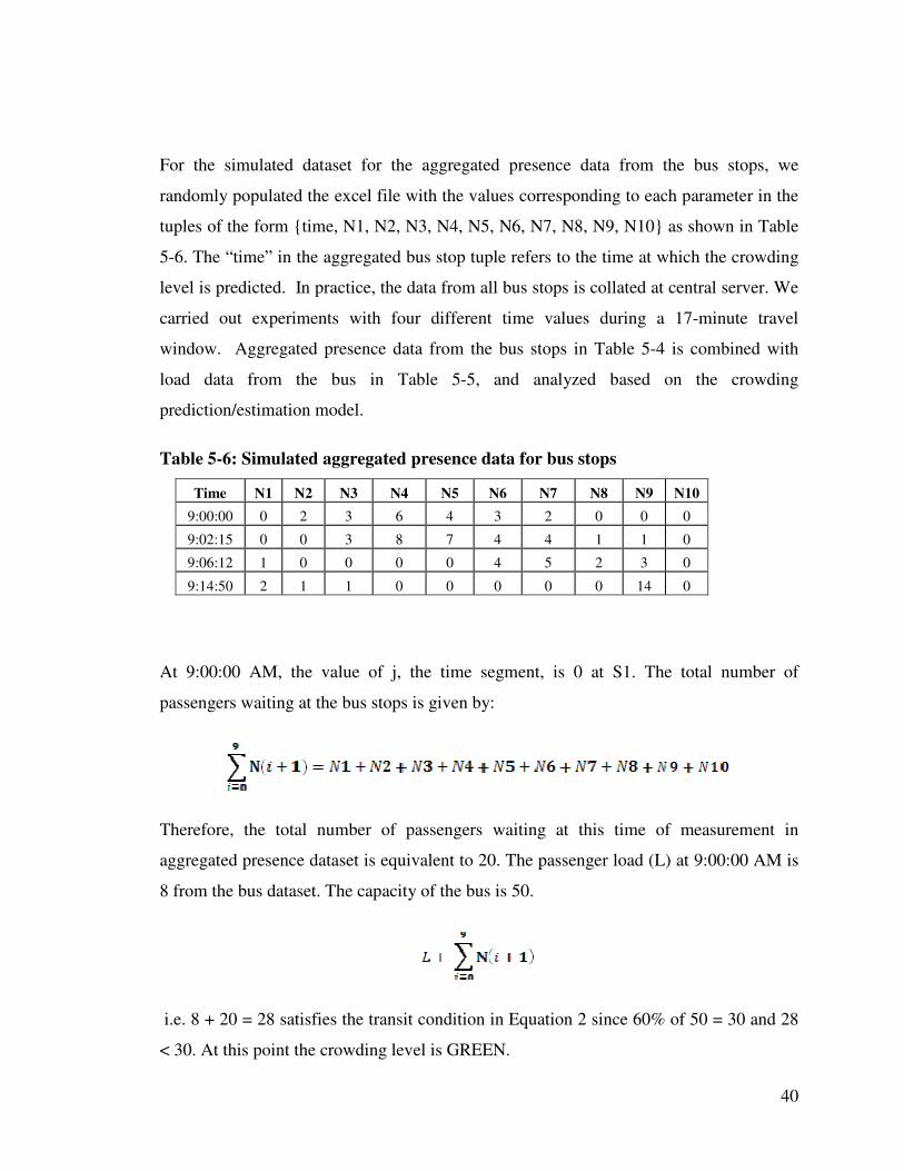
At 9:00:00 AM, the value of j, the time segment, is 0 at S1. The total number of
passengers waiting at the bus stops is given by:
Therefore, the total number of passengers waiting at this time of measurement in
aggregated presence dataset is equivalent to 20. The passenger load (L) at 9:00:00 AM is
8 from the bus dataset. The capacity of the bus is 50.
i.e. 8 + 20 = 28 satisfies the transit condition in Equation 2 since 60% of 50 = 30 and 28
< 30. At this point the crowding level is GREEN.
41
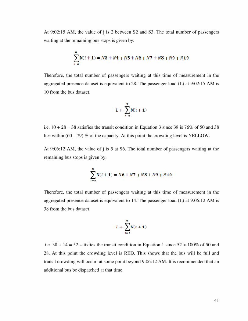
At 9:02:15 AM, the value of j is 2 between S2 and S3. The total number of passengers
waiting at the remaining bus stops is given by:
Therefore, the total number of passengers waiting at this time of measurement in the
aggregated presence dataset is equivalent to 28. The passenger load (L) at 9:02:15 AM is
10 from the bus dataset.
i.e. 10 + 28 = 38 satisfies the transit condition in Equation 3 since 38 is 76% of 50 and 38
lies within (60 – 79) % of the capacity. At this point the crowding level is YELLOW.
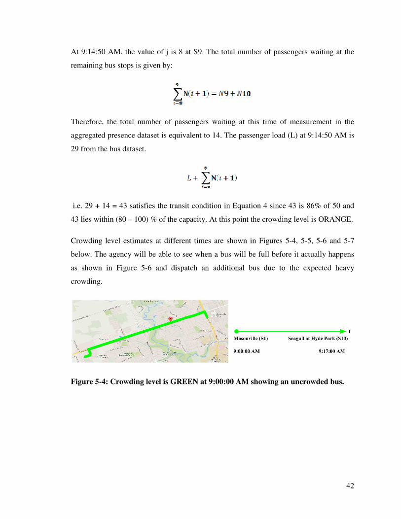
At 9:06:12 AM, the value of j is 5 at S6. The total number of passengers waiting at the
remaining bus stops is given by:
Therefore, the total number of passengers waiting at this time of measurement in the
aggregated presence dataset is equivalent to 14. The passenger load (L) at 9:06:12 AM is
38 from the bus dataset.
i.e. 38 + 14 = 52 satisfies the transit condition in Equation 1 since 52 > 100% of 50 and
28. At this point the crowding level is RED. This shows that the bus will be full and
transit crowding will occur at some point beyond 9:06:12 AM. It is recommended that an
additional bus be dispatched at that time.
42
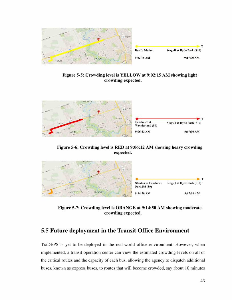
At 9:14:50 AM, the value of j is 8 at S9. The total number of passengers waiting at the
remaining bus stops is given by:
Therefore, the total number of passengers waiting at this time of measurement in the
aggregated presence dataset is equivalent to 14. The passenger load (L) at 9:14:50 AM is
29 from the bus dataset.
i.e. 29 + 14 = 43 satisfies the transit condition in Equation 4 since 43 is 86% of 50 and
43 lies within (80 – 100) % of the capacity. At this point the crowding level is ORANGE.
Crowding level estimates at different times are shown in Figures 5-4, 5-5, 5-6 and 5-7
below. The agency will be able to see when a bus will be full before it actually happens
as shown in Figure 5-6 and dispatch an additional bus due to the expected heavy
crowding.
Figure 5-4: Crowding level is GREEN at 9:00:00 AM showing an uncrowded bus.
43
Figure 5-5: Crowding level is YELLOW at 9:02:15 AM showing light
crowding expected.
Figure 5-6: Crowding level is RED at 9:06:12 AM showing heavy crowding
expected.
Figure 5-7: Crowding level is ORANGE at 9:14:50 AM showing moderate
crowding expected.
5.5 Future deployment in the Transit Office Environment
TraDEPS is yet to be deployed in the real-world office environment. However, when
implemented, a transit operation center can view the estimated crowding levels on all of
the critical routes and the capacity of each bus, allowing the agency to dispatch additional
buses, known as express buses, to routes that will become crowded, say about 10 minutes
44
ahead from the time measured. The transit office receives notification messages for the
different crowding levels at a given time. Customers are also informed of potential
crowding in the future and the best alternative routes via mobile applications and the
web. The results are computed using real-time data analytics powered by TraDEPS in
combination with the crowding prediction model discussed in Chapter 3. This is likely to
provide efficient usage of the transit vehicles while preventing the incidence of crowding
rather than just increasing the frequencies of services on a route to prevent overcrowding.
45
Chapter 6
6 DISCUSSION
6.1 Benefits for Public Transit Management
The main goal behind the transit analytics, predictions and visualizations is to provide
alerts and a view of the near future crowding level to the transit managers so that action
can be taken before transit crowding occurs. It also provides customers with smartphones
and access to the web about crowding in the future and the best alternative routes. It is
non-intrusive since it does not require the installation of an application from an
application repository on a smartphone and does not impact the performance of the
smartphones e.g. draining the battery.
6.2 Drawbacks
Smartphone Penetration
If every passenger waiting at the stop were carrying a smartphone, calculating the
statistics on number of waiting passengers would be very easy. Smartphone penetration
by percentage in different countries is usually published but this may vary very widely
for each bus stop on a specific route. This may not give accurate results when
ascertaining the actual number of passengers present or waiting at each bus stop based on
the devices.
46
Multiple Routes
The system works best if there is only one route at each stop. However, there may be
several routes for a particular bus stop. As a result, the data collected may be tainted and
inaccurate.
Perception of Privacy
It is possible that many transit riders that own devices are not aware of being tracked by
the system. Once they are aware, then the notion of privacy may become very important
to them. Some riders may not feel comfortable if their digital presence is being tracked as
they may think their personal information is being collected or phone hacked.
Re-Identification
Data that is anonymized may be re-identified thereby revealing the privacy of the riders.
Wi-Fi State
Wi-Fi must be enabled on the rider’s smartphone for the Wi-Fi node to be able to collect
data from the rider. Some riders may be uncomfortable with data being collected and
disable the Wi-Fi on their smartphones. Turning off Wi-Fi by a rider to conserve battery
and extend the battery life of a smartphone is also possible.
47
Chapter 7
7 CONCLUSIONS AND FUTURE WORK
7.1 Conclusions
Real-time transit data can now be collected and data visualization of transit conditions
provided based on Wi-Fi sensors that can track smart devices equipped with Wi-Fi. This
is especially helpful for public transit managers for decision-making before transit
crowding actually occur.
Leveraging on distributed tracking and monitoring, the transit demand estimation and
prediction system, an end-to-end system, can aggregate data from many Wi-Fi sensors
deployed across different bus stops and routes and time periods. Combining the data
feeds with data from other sources provides for effective analysis and presentation of this
data for transit management.
With this approach to transit management, there is a need to ensure the privacy of riders.
Security measures are maintained by encrypting data before transmission, making sure
the MAC address data is anonymized and modified to an extent where it is very difficult
to derive the initial MAC address. By addressing privacy concerns and building a
scalable system that can be used in many stop locations and public transit, municipal
transit agencies can look forward to providing information about transit conditions in
real-time and better management of transit crowding.
48
7.2 Contributions
In our work, we describe our aproach for estimating passenger demand based on real-
time data. We created a modular system for sensing devices and discovering passenger
presence at the bus stops, counting and collating the presence data on a central server. We
have shown that our approach is useful in discovering passenger presence in the
condition of constrained and practical deployment requirements.
We proposed a crowding prediction model for a transit demand estimation and prediction
system (TraDEPS) to reveal when the bus will be full or crowded during a trip. We have
shown that crowding levels can be predicted/estimated using simple prediction model
based on real-time data although crowding is known to be pretty random. The results
suggest that the model may be appropriate for deployment to determine when the transit
vehicle will become crowded at a transit operations center. It can provide several minutes
of advance notice before crowding will occur. This several minutes of warning may allow
managers and staff members to take action to alleviate crowding. Possible action includes
the dispatch of an additional bus. In addition, the results show that analysis information
concerning crowding levels can be included in the Advanced Traveller Information
Systems (ATIS) to provide advice to the transit riders ahead of time.
7.3 Limitations
The present work has a limitation that merit discussion. Because we have used simulated
data instead of real data, it is difficult to validate how succesful this approach to reveal
transit crowding will be if the devices were deployed in the real-world. Due to the
drawbacks inherent in this approach, it may be difficult to get an accurate count of the
people at the bus stops. The worst case scenario would be that no one comes along to a
bus stop with a smartphone device.
49
7.4 Future Work
Future extensions of the present work might include assessing the impact of weather,
historical data, events, social media data, locales and traffic on the implementation taking
the following into consideration:
• Live bus arrival data feed
• Historical data of the number of riders on a bus
• Historical data of the passenger demand on different routes
• Local events data: Municipality events information (location, event type,
description, category)
• Commercial venue data: categorization and descriptions of all commercial
venues, including GPS locations.
• Hourly weather data: temperature, temperature with wind chill, rain/sun/snow
• Facebook stream: all geocoded posts within a municipality
• Google+ stream: all geocoded posts within a municipality
• Tweet stream: all geocoded tweets within a municipality
• Central server sending notification message to the transit operations sender and
clients when the bus will be full.
Compared to real-world data, simulated data used in the analysis are generally ideal but
lack practicability. With real-world data, the prediction model could be tested and
improved to ensure overall prediction results with a very high percentage of accuracy. A
better prediction model or sophisticated algorithm could be developed in the future for
crowding predictions. This could include factors such as time, distance, and aggregated
volumes of waiting passengers about two to four bus stops away from the current location
of the bus as well as the aggregated volumes of waiting passengers near the end of the
trip. The techniques of encryption, decryption, compression and decompression could be
implemented in the future to make the system more robust.
50
8. BIBLIOGRAPHY
[1] Veitch, T., J. Partridge, and L. Walker: "Estimating the costs of over-crowding on
Melbourne's rail system." Australasian Transport Research Forum (ATRF), 36th, 2013,
Brisbane, Queensland, Australia, pp. 1, 2013 [Online]
http://www.atrf.info/papers/2013/2013_veitch_partridge_walker.pdf, Accessed July
2014.
[2] Qin, Feifei: "Investigating the In-vehicle Crowding Cost Functions for Public Transit
Modes", Mathematical Problems in Engineering, vol. 2014, Article ID 502708, 13 pages,
pp. 8, 2014. doi:10.1155/2014/502708 [Online]
http://www.hindawi.com/journals/mpe/2014/502708/. Accessed July 2014
[3] Google Maps traffic (https://www), [Online]
support.google.com/maps/answer/3093389/ website. Accessed June 2014
[4] Measuring transit demand (http://www),
[Online] en.wikibooks.org/wiki/Fundamentals_of_Transportation/Transit_Demand/
website. Accessed June 2014
[5] Healy, R., Kapilian, R.: Passenger Counting and Service Monitoring, pp. 9, 2003,
(http://wwww) [Online] ntl.bts.gov/lib/23000/23600/23620/psgr_ctg_svc_mon.pdf,
website. Accessed July 2014
[6] Fuerstenberg, K.C., Dietmayer, K.C.J., Willhoeft, V.: ‘Pedestrian recognition in
urban traffic using a vehicle based multilayer laser scanner’. IEEE Intelligent Vehicle
Symp., vol. 1, pp. 31–35, June 2002.
[7] Oberli, C., Torres-Torriti, M., Landau, D.: ‘Performance evaluation of UHF RFID
technologies for real-time passenger recognition in intelligent public transportation
systems’, IEEE Trans. Intell. Transp. Syst., vol. 11, issue 3, pp. 748–753, 2010.
[8] Bi, L., Tsimhoni, O., Liu, Y.: ‘Using image-based metrics to model pedestrian
detection performance with night-vision systems’, IEEE Trans. Intell. Transp. Syst., vol.
10, issue 1, pp. 155–164, 2009.
51
[9] Kilambi, Prahlad, et al.: "Estimating pedestrian counts in groups." Computer Vision
and Image Understanding 110.1, pp. 43-59, 2008 doi: 10.1016/j.cviu.2007.02.003.
[10] CRTC issues annual report on the state of the Canadian communication system
(https://www), [Online] crtc.gc.ca/eng/com100/2013/r130926.htm/ website. Accessed
July 2014
[11] Canadian Smartphone Adoption at 62% comScore says (https://www), [Online]
iphoneincanada.ca/news/canadian-smartphone-adoption-at-62-comscore-says/ website.
Accessed July 2014.
[12] Raspberry PI (https://www), [Online] raspberrypi.org/ website. Accessed July
2014.
[13] Arduino (https://www), [Online] arduino.cc website. Accessed July 2014.
[14] Torres, Neftali: "Advance Traveler Information Systems." (2008). (https://www),
[Online] its-ct.org/documents/StudentGrant/ATISreport2008-09.pdf Accessed July 2014.
[15] Navick, D. and Furth, P.: Estimating Passenger Miles, Origin-Destination Patterns,
and Loads with Location Stamped Farebox Data, Transportation Research Record, 1799,
pp. 107-113, 2002.
[16] Travlink Operational Test Evaluation Report, Minnesota Department of
Transportation, Guidestar Office, pp. 1, 1996, (https://www), [Online]
ntl.bts.gov/lib/jpodocs/repts_te/2583.pdf website. Accessed July 2014.
[17] Bruce Wetherby: "Seattle Wide-Area Information for Travelers (SWIFT):
Evaluation Summary." Science Applications International Corporation, pp. 5, 1998,
(https://www), [Online] ntl.bts.gov/lib/jpodocs/repts_te/7404.pdf website. Accessed July
2014.
[18] Ferris, Brian, Kari Watkins, and Alan Borning: "Location-aware tools for
improving Public transit Usability." IEEE Pervasive Computing 9.1, pp. 13-19, 2010.
52
[19] TCRP Report 58: New paradigms for Local Public Transportation Organizations –
Task 5 Report: Opening the Door to Fundamental Change, Transportation Research
Board of the National Academies, Washington, DC: pp. 15, 2000, (https://www),
[Online] tcrponline.org/PDFDocuments/tcrp_rpt_58.pdf website. Accessed July 2014.
[20] Markovic, H., Basic, B.D., Gold, H., Dong, F., Hirota, K.: GPS data-based non-
parametric regression for predicting travel time in urban traffic networks. Sci. Traffic
Transport vol. 22, issue 1, pp. 1–13, 2010.
[21] Wu, C.H., Ho, J.M., Lee, D.T.: Travel-time prediction with support vector
regression. IEEE Trans. Intell. Transportation System 5(4), pp. 276–281, 2004.
[22] Zhang, X., Rice, J.A.: Rice. "Short-term travel time prediction." Transportation
Research Part C: Emerging Technologies 11, no. 3 (2003): 187-210.
[23] Rzeszotko, J., Nguyen, S.H.: Machine learning for traffic prediction. Fundam. Inf
119(3-4), pp. 407–420, 2012.
[24] Dunne, S., Ghosh, B.: Weather adaptive traffic prediction using neurowavelet
models. IEEE Trans. Intell. Transportation Syst 14(1), pp. 370–379, 2013.
[25] Mazloumi, E., Rose, G., Currie, G., Moridpour, S.: Prediction intervals to
account for uncertainties in neural network predictions: methodology and application in
bus travel time prediction. Eng. Appl. Artif. Intell 24(3), pp. 534–542, 2011.
[26] van Hinsbergen, C.P.I.J., Hegyi, A., van Lint, J.W.C., van Zuylen, H.J.:
Bayesian neural networks for the prediction of stochastic travel times in urban networks.
IET Intell. Transport Syst 5(4), pp. 259–265, 2011.
[27] Comert, G., Bezuglov, A.: An online change-point-based model for traffic
parameter prediction. IEEE Trans. Intell. Transportation Syst 14(3), pp. 1360–1369,
2013.
[28] Min, W., Wynter, L.: Real-time road traffic prediction with spatio-temporal
correlations. Transportation Res. Part C 19, pp. 606–616, 2011.
53
[29] Xia, J., Chen, M., Huang, W.: A multistep corridor travel-time prediction method
using presence-type vehicle detector data. J. Intell. Transportation Syst: Technol. Plann.
Oper 15(2), pp. 104–113, 2011.
[30] Vijayan, V.P., Paul, B.: Multi objective traffic prediction using type-2 fuzzy logic
and ambient intelligence. Proceedings of 2010 International Conference on Advances in
Computer Engineering (ACE), pp. 309–311, 2010
[31] Li, L., Lin, W.H., Liu, H.: Type-2 fuzzy logic approach for short-term traffic
forecasting. IEE Proc. Intell. Transport Syst 153(1), pp. 33–40, 2006.
[32] Ghosh, B., Basu, B., O’Mahony, M.: Multivariate short-term traffic flow
forecasting using time-series analysis. IEEE Trans. Intell. Transportation Syst 10(2), pp.
246–254, 2009.
[33] Smith, B.L., Williams, B.M., Oswalsd, R.K.: Comparison of parametric and
nonparametric models for traffic flow forecasting. Transportation Res. Part C 10(4), pp.
303–321, 2002.
[34] Wang, Y., Papageorgiou, M.: A Messmer, Real-time freeway traffic state
estimation based on extended kalman filter: a case study. Transportation Sci 4(2), pp.
167–181, 2007.
[35] Chen, M., Chien, S.I.J.: Dynamic freeway travel-time prediction with probe vehicle
data: link based versus path based. Transportation Res. Rec 1768, pp. 157–161, 2001.
[36] Ahn K., Rakha H., Hill D.: Data quality white paper. No. fhwa-HOP-08-038. US
Department of Transportation, Federal Highway Administration, pp. 14-15, 2008.
[37] Balmer, M., Nagel, K., Raney, B.: "Large-scale multi-agent simulations for
transportation applications." Intelligent Transportation Systems. Vol. 8. No. 4. Taylor &
Francis Group, pp. 1-16, 2004.
[38] Payne, H.J.: "FREFLO: A macroscopic simulation model of freeway traffic."
Transportation Research Record 722, pp. 68-77, 1979.
54
[39] IEEE OUI Registry (https://), [Online]
standards.ieee.org/develop/regauth/oui/oui.txt. website. Accessed July 2014.
[40] Wireshark (https://www), [Online] wireshark.org website. Accessed July 2014.
[41] Google Maps (https://www), google.com/mobile/maps website. Accessed July 2014
[42] Wireless Networks (https://www),
technologyuk.net/telecommunications/networks/wireless_networks.shtml website.
Accessed July 2014
[43] Ramesh, G., Umarani, R.: "Performance Analysis of Most Common Encryption
Algorithms on Different Web Browsers." International Journal of Information
Technology and Computer Science (IJITCS) 4.12 (2012): 60.

55
Curriculum Vitae
Name: Michael Aro
Post-secondary VAMK – Vaasan ammattikorkeakoulu
Education and Vaasa, Finland
Degrees: BEng, Information Technology
Honours and Western Graduate Research Scholarship
Awards: 2012–2013
Related Work Teaching Assistant
Experience Western University
2012-2013