Transition Densities for Interest Rate and Other Nonlinear ...yacine/trans.pdft is a stochastic differential equation, dX t 5 m~X t;u!dt 1 s~X t;u!dW t, ~1! where W t is a standard

Transition Densities for Interest Rateand Other Nonlinear Diffusions

YACINE AÏT-SAHALIA*

ABSTRACT

This paper applies to interest rate models the theoretical method developed inAït-Sahalia ~1998! to generate accurate closed-form approximations to the transi-tion function of an arbitrary diffusion. While the main focus of this paper is on themaximum-likelihood estimation of interest rate models with otherwise unknowntransition functions, applications to the valuation of derivative securities are alsobrief ly discussed.

CONTINUOUS-TIME MODELING IN FINANCE, though introduced by Louis Bachelier’s1900 thesis on the theory of speculation, really started with Merton’s sem-inal work in the 1970s. Since then, the continuous-time paradigm has provedto be an immensely useful tool in finance and more generally economics.Continuous-time models are widely used to study issues that include thedecision to optimally consume, save, and invest, portfolio choice under avariety of constraints, contingent claim pricing, capital accumulation, re-source extraction, game theory, and more recently contract theory. Manyrefinements and extensions are possible, but the basic dynamic model forthe variable~s! of interest Xt is a stochastic differential equation,

dXt 5 m~Xt ;u!dt 1 s~Xt ;u!dWt , ~1!

where Wt is a standard Brownian motion and the drift m and diffusion s2

are known functions except for an unknown parameter1 vector u in a boundedset Q , Rd.

One major impediment to both theoretical modeling and empirical workwith continuous-time models of this type is the fact that in most cases littlecan be said about the implications of the dynamics in equation ~1! for longer

*Department of Economics, Princeton University. Mathematica code to implement this methodcan be found at http:00www.princeton.edu0;yacine. I am grateful to David Bates, René Car-mona, Freddy Delbaen, Ron Gallant, Lars Hansen, Per Mykland, Peter C. B. Phillips, PeterRobinson, Angel Serrat, Suresh Sundaresan, and George Tauchen for helpful comments. RobertKimmel provided excellent research assistance. This research was conducted during the au-thor’s tenure as an Alfred P. Sloan Research Fellow. Financial support from the NSF ~GrantSBR-9996023! is gratefully acknowledged.

1 Non- and semiparametric approaches, which do not constrain the functional form of thefunctions m and0or s2 to be within a parametric class, have been developed ~see Aït-Sahalia~1996a, 1996b! and Stanton ~1997!!.

THE JOURNAL OF FINANCE • VOL. LIV, NO. 4 • AUGUST 1999

1361

time intervals. Though equation ~1! fully describes the evolution of the vari-able X over each infinitesimal instant, one cannot in general characterize inclosed form an object as simple ~and fundamental for everything from pre-diction to estimation and derivative pricing! as the conditional density ofXt1D given the current value Xt . For a list of the rare exceptions, see Wong~1964!. In finance, the well-known models of Black and Scholes ~1973!, Va-sicek ~1977!, and Cox, Ingersoll, and Ross ~1985! rely on these existing closed-form expressions. In this paper, I describe and implement empirically a methoddeveloped in a companion paper ~Aït-Sahalia ~1998!! which produces veryaccurate approximations in closed form to the unknown transition functionpX~D, x 6x0;u!, the conditional density of Xt1D 5 x given Xt 5 x0 implied bythe model in equation ~1!.

These closed-form expressions can be useful for at least two purposes.First, they let us estimate the parameter vector u by maximum-likelihood.2

In most cases, we observe the process at dates $t 5 iD6i 5 0, . . . , n% , whereD . 0 is generally small, but fixed as n increases. For instance, the seriescould be weekly or monthly. Collecting more observations means lengthen-ing the time period over which data are recorded, not shortening the timeinterval between successive existing observations.3 Because a continuous-time diffusion is a Markov process, and that property carries over to anydiscrete subsample from the continuous-time path, the log-likelihood func-tion has the simple form

,n~u! [ n21 (i51

n

ln$ pX ~D, XiD 6X~i21!D ;u!%. ~2!

With a given D, two methods are available in the literature to compute pXnumerically. They involve either solving numerically the Kolmogorov partialdifferential equation known to be satisfied by pX ~see, e.g., Lo ~1988!!, orsimulating a large number of sample paths along which the process is sam-pled very finely ~see Pedersen ~1995!, Honoré ~1997!, and Santa-Clara ~1995!!.Neither method however produces a closed-form expression to be maximized

2 A large number of new approaches have been developed in recent years. Some theoreticalestimation methods are based on the generalized method of moments ~Hansen and Scheinkman~1995! and Bibby and Sørenson ~1995!! and on nonparametric density-matching ~Aït-Sahalia~1996a, 1996b!!, others are based on nonparametric approximate moments ~Stanton ~1997!!,simulations ~Duffie and Singleton ~1993!, Gouriéroux, Monfort, and Renault ~1993!, Gallantand Tauchen ~1998!, and Pedersen ~1995!!, the spectral decomposition of the infinitesimal gen-erator ~Hansen, Scheinkman, and Touzi ~1998! and Florens, Renault, and Touzi ~1995!!, randomsampling of the process to generate moment conditions ~Duffie and Glynn ~1997!!, or, finally,Bayesian approaches ~Eraker ~1997!, Jones ~1997!, and Elerian, Chib, and Shephard ~1998!!.

3 Discrete approximations to the stochastic differential equation ~1! could be employed ~seeKloeden and Platen ~1992!!: see Chan et al. ~1992! for an example. As discussed by Merton~1980!, Lo ~1988!, and Melino ~1994!, ignoring the difference generally results in inconsistentestimators, unless the discretization happens to be an exact one, which is tantamount to sayingthat pX would have to be known in closed form.

1362 The Journal of Finance

over u, and the calculations for all the pairs ~x, x0! must be repeated sepa-rately every time the value of u changes. By contrast, the closed-form ex-pressions in this paper make it possible to maximize the expression in equation~2! with pX replaced by its closed-form approximation.

Derivative pricing provides a second natural outlet for applications of thismethodology. Suppose that we are interested in pricing at date zero a de-rivative security written on an asset with price process $Xt 6t $ 0% , and withpayoff function C~XD! at some future date D. For simplicity, assume that theunderlying asset is traded, so that its risk-neutral dynamics have the form

dXt 0Xt 5 $r 2 d%dt 1 s~Xt ;u!dWt , ~3!

where r is the riskfree rate and d is the dividend rate paid by the asset—both constant again for simplicity.

It is well known that when markets are dynamically complete, the onlyprice of the derivative security that is compatible with the absence of arbi-trage opportunities is

P0 5 e2rDE @C~XD!6X0 5 x0# 5 e2rDE0

1`

C~x!pX ~D, x 6x0;u! dx, ~4!

where pX is the transition function ~or risk-neutral density, or state-pricedensity! induced by the dynamics in equation ~3!.

The Black–Scholes option pricing formula is the prime example of equa-tion ~4!, when s~Xt ;u! 5 s is constant. The corresponding pX is known inclosed-form ~as a lognormal density! and so the integral in equation ~4! canbe evaluated explicitly for specific payoff functions ~see also Cox and Ross~1976!!. In general, of course, no known expression for pX is available andone must rely on numerical methods such as solving numerically the PDEsatisfied by the derivative price, or Monte Carlo integration of equation ~3!.These methods are the exact parallels to the two existing approaches tomaximum-likelihood estimation that I described earlier.

Here, given the sequence $ IpX~K ! 6K $ 0% of approximations to pX , the valu-

ation of the derivative security would be based on the explicit formula

P0~K !

5 e2rDE0

1`

C~x! IpX~K !

~D, x 6x0;u! dx. ~5!

Formulas of the type given in equation ~4! where the unknown pX is re-placed by another density have been proposed in the finance literature ~see,e.g., Jarrow and Rudd ~1982!!. There is an important difference, however,between what I propose and the existing formulas: the latter are based oncalculating the integral in equation ~4! with an ad hoc density &pX—typicallyadding free skewness and kurtosis parameters to the lognormal density, so

Transition Densities for Interest Rate and Other Diffusions 1363

as to allow for departures from the Black–Scholes formula. In doing so, theseformulas ignore the underlying dynamic model specified in equation ~3! forthe asset price, whereas my method gives in closed form the option pricingformula ~of order of precision corresponding to that of the approximationused! that corresponds to the given dynamic model in equation ~3!. Then onecan, for instance, explore how changes in the specification of the volatilityfunction s~x;u! affect the derivative price, which is obviously impossible whenthe specification of the density &pX to be used in equation ~4! in lieu of pX isunrelated to equation ~3!.

The paper is organized as follows. In Section I, I brief ly describe the ap-proach used in Aït-Sahalia ~1998! to derive a closed-form sequence of ap-proximations to pX , give the expressions for the approximation, and describeits properties. In Section II, I study a number of interest rate models, somewith unknown transition functions, and give the closed-form expressions ofthe corresponding approximations. Section III reports maximum-likelihoodestimates for these models using the Federal funds rate, sampled monthlyfrom 1963 through 1998. Section IV concludes, and a statement of the tech-nical assumptions is in the Appendix.

I. Closed-Form Approximations to the Transition Function

A. Tail Standardization via Transformation to Unit Diffusion

The first step toward constructing the sequence of approximations to pXconsists of standardizing the diffusion function of X—that is, transforming Xinto another diffusion Y defined as

Yt [ g~Xt ;u! 5EXt

du0s~u;u!, ~6!

where any primitive of the function 10s may be selected.Let DX 5 ~ tx, Sx! denote the domain of the diffusion X. I will consider two

cases, where DX 5 ~2`,1`! or DX 5 ~0,1`!. The latter case is often relevantin finance, when considering models for asset prices or nominal interestrates. Moreover, the function s is often specified in financial models in sucha way that s~0;u! 5 0 and m and0or s violates the linear growth conditionsnear the boundaries. The assumptions in the Appendix allow for this behavior.

Because s . 0 on the interior of the domain DX , the function g in equation~6! is increasing and thus invertible. It maps DX into DY 5 ~ ry, Sy!, the domainof Y. For a given model under consideration, I will assume that the param-eter space Q is restricted in such a way that DY is independent of u in Q.This restriction on Q is inessential, but it helps keep the notation simple.Again, in finance, most, if not all cases, will have DX and DY be either thewhole real line ~2`,1`! or the half line ~0,1`!.


By applying Itô’s Lemma, Y has unit diffusion as desired:

dYt 5 mY ~Yt ;u!dt 1 dWt , ~7!

where

mY ~ y;u! 5m~g21~ y;u!;u!

s~g21~ y;u!;u!2

1

2

?s

?x~g21~ y;u!;u!. ~8!

Finally, note that it can be convenient to define Yt instead as minus theintegral in equation ~6! if that makes Yt . 0, for instance if s~x;u! 5 x r

and r . 1. For example, if DX 5 ~0,1`! and s~x;u! 5 x r, then Yt 5~1 2 r!Xt

12r if 0 , r , 1 ~so DY 5 ~0,1`!!, Yt 5 ln~Xt! if r 5 1 ~soDY 5 ~2`,1`!!, and Yt 5 ~ r 2 1!Xt

2~ r21! if r . 1 ~so DY 5 ~0,1`! again!.In all cases, Y has unit diffusion; that is, sY

2~ y;u! 5 1. When the transfor-mation Yt [ g~Xt ;u! 5 2*Xt du0s~u;u! is used, the drift mY~ y;u! indYt 5 mY~Yt ;u!dt 2 dWt is, instead of equation ~8!,

mY ~ y;u! 5 2m~g21~ y;u!;u!

s~g21~ y;u!;u!1

1

2

?s

?x~g21~ y;u!;u!. ~9!

The point of making the transformation from X to Y is that it is possibleto construct an expansion for the transition density of Y. Of course, thiswould be of little interest because we only observe X, not the artificiallyintroduced Y, and the transformation depends on the unknown parametervector u. However, the transformation is useful because one can obtain thetransition density pX from pY through the Jacobian formula

pX ~D, x 6x0;u! 5?

?xProb~Xt1D # x 6Xt 5 x0;u!

5?

?xProb~Yt1D # g~x;u!6Yt 5 g~x0;u!;u!

5?

?x FEryg~x;u!

pY ~D, y 6g~ y0;u!;u!dyG5

pY ~D,g~x;u!6g~x0;u!;u!

s~g~x;u!;u!. ~10!

Therefore, there is never any need to actually transform the data $XiD, i 50, . . . , n% into observations on Y ~which depends on u anyway!. Instead, thetransformation from X to Y is simply a device to obtain an approximation


for pX from the approximation of pY . Practically speaking, when the ap-proximation for pX has been derived once and for all as the Jacobian trans-form of that of Y, the process Y no longer plays any role.

B. Explicit Expressions for the Approximation

As shown in Aït-Sahalia ~1998!, one can derive an explicit expansion forthe transition density of the variable Y based on a Hermite expansion of itsdensity y ° pY~D, y 6y0;u! around a Normal density function. The analyticpart of the expansion of pY up to order K is given by

IpY~K !

~D, y 6y0;u! 5 D2102fS y 2 y0

D102 DexpSEy0

y

mY ~w;u!dwD(k50

K

ck~ y 6y0;u!Dk

k!,

~11!

where f~z! [ e2z2020%2p denotes the N~0,1! density function, c0~ y 6y0;u! 5 1,and for all j $ 1,

cj ~ y 6y0;u! 5 j~ y 2 y0!2jEy0

y

~w 2 y0! j21

3 $lY ~w!cj21~w 6y0;u! 1 ~?2cj21~w 6y0;u!0?w2 !02% dw, ~12!

where lY~ y;u! [ 2~mY2 ~ y;u! 1 ?mY~ y;u!0?y!02.

Tables I through V give the explicit expression of these coefficients forpopular models in finance, which I discuss in detail in Section II. Beforeturning to these examples, a few general remarks are in order. The generalstructure of the expansion in equation ~11! is as follows: The leading term inthe expansion is Gaussian, D2102f~~ y 2 y0!0D102 !, followed by a correction forthe presence of the drift, exp~*y0

y mY ~w;u! dw! , and then additional correctionterms that depend on the specification of the function lY~ y;u! and its suc-cessive derivatives. These correction terms play two roles: they account forthe nonnormality of pY and they correct for the discretization bias implicit instarting the expansion with a Gaussian term with no mean adjustment andvariance D ~instead of Var@Yt1D6Yt# , which is equal to D only in the firstorder!.

In general, the function pY is not analytic in time. Therefore equation ~11!must be interpreted strictly as the analytic part, or Taylor series. In partic-ular, for given ~ y, y0,u! it will generally have a finite convergence radius inD. As we will see below, however, the series in equation ~11! with K 5 1 or 2at most is very accurate for the values of D that one encounters in empiricalwork in finance.


The sequence of explicit functions IpY~K ! in equation ~11! is designed to ap-

proximate pY . As discussed above, one can then approximate pX ~the objectof interest! by using the Jacobian formula for the inverted change of vari-able Y r X:

IpX~K !

~D, x 6x0;u! [ s~x;u!21 IpY~K !

~D,g~x;u!6g~x0;u!;u!. ~13!

The main objective of the transformation X r Y was to provide a methodof controlling the size of the tails of the transition density. As shown inAït-Sahalia ~1998!, the fact that Y has unit diffusion makes the tails of thedensity pY , in the limit where D goes to zero, similar in magnitude to thoseof a Gaussian variable. That is, the tails of pY behave like exp@2y202D# asis apparent from equation ~11!. However, the tails of the density pX areproportional to exp@2g~x;u!202D# . So, for instance, if s~x;u! 5 2!x theng~x;u! 5 !x and the right tail of pX becomes proportional to exp@2x 202D# ;this is verified by equation ~13!. Not surprisingly, this is the tail behaviorfor Feller’s transition density in the Cox, Ingersoll, and Ross ~1985! model.If now s~x;u! 5 x, then g~x;u! 5 ln~x! and the tails of pX are proportionalto exp@2ln~x! 202D#: this is what happens in the log-Normal case ~see theBlack–Scholes model!. In other words, while the leading term of the expan-sion in equation ~11! for pY is Gaussian, the expansion for pX will startwith a deformed or “stretched” Gaussian term, with the specific form ofthe deformation given by the function g~x;u!.

The sequence of functions in equation ~11! solves the forward and back-ward Kolmogorov equations up to order DK ; that is,

5? IpY

~K !

?D1?

?y$mY ~ y;u! IpY

~K !% 2

1

2

?2 IpY~K !

?y2 5 O~DK !

? IpY~K !

?D2 mY ~ y0;u!

? IpY~K !

?y02

1

2

?2 IpY~K !

?y02 5 O~DK !

. ~14!

The boundary behavior of the transition density IpY~K ! is similar to that of pY ;

under the assumptions made, limyr ry or Sy pY 5 0. The expansion is designed todeliver an approximation of the density function y ° pY~D, y 6y0;u! for a fixedvalue of conditioning variable y0. Therefore, except in the limit where Dbecomes infinitely small, it is not designed to reproduce the limiting behav-ior of pY in the limit where y0 tends to the boundaries.

Finally, note that the form of the expansion is compatible with the expres-sion that arises out of Girsanov’s Theorem in the following sense. Under theassumptions made, the process Y can be transformed by Girsanov’s Theoreminto a Brownian motion if DY 5 ~2`,1`!, or into a Bessel process in dimen-sion 3 if DY 5 ~0,1`!. This gives rise to a formulation of pY in a form thatinvolves the conditional expectation of the exponential of the integral of func-


tion of a Brownian Bridge ~see Gihman and Skorohod ~1972, Chap. 3! for thecase where DY 5 ~2`,1`!!, or a Bessel Bridge if DY 5 ~0,1`!. This condi-tional expectation term can either be expressed in terms of the conditionaldensities of the Brownian Bridge when DY 5 ~2`,1`! ~see Dacunha-Castelle and Florens-Zmirou ~1986!!, or integrated by Monte Carlo simula-tion. Further discussion of these and other theoretical properties of theexpansion is contained in Aït-Sahalia ~1998!.

II. Examples

A. Comparison of the Approximation to the Closed-Form Densitiesfor Specific Models

In this section, I study the size of the approximation made when replacingpX by IpX

~K ! , in the case of typical examples in finance where pX is known inclosed form and sampling is at the monthly frequency. Since the perfor-mance of the approximation improves as D gets smaller, monthly sampling istaken to represent a worst-case scenario as the upper bound to the samplinginterval relevant for finance. In practice, most continuous-time models infinance are estimated with monthly, weekly, daily, or higher frequency ob-servations. The examples studied below reveal that including the termc2~ y, y0;u! generally provides an approximation to pX which is better by afactor of at least 10 than what one obtains when only the term c1~ y, y0;u! isincluded. Further calculations show that each additional order produces ad-ditional improvements by an additional factor of at least 10.

I will often compare the expansion in this paper to the Euler approxima-tion; the latter corresponds to a simple discretization of the continuous-timestochastic differential equation, where the differential equation ~1! is re-placed by the difference equation

Xt1D 2 Xt 5 m~Xt ;u!D 1 s~Xt ;u!%Det1D ~15!

with et1D ; N~0,1!, so that

pXEuler~D, x 6x0;u! 5 ~2pDs2~x0;u!!2102

3 exp $2~x 2 x0 2 m~x0;u!D!202Ds2~x0;u!%. ~16!

Example 1 (Vasicek’s Model): Consider the Ornstein–Uhlenbeck specifica-tion proposed by Vasicek ~1977! for the short-term interest rate:

dXt 5 k~a 2 Xt !dt 1 sdWt . ~17!

X is distributed on DX 5 ~2`,1`! and has the Gaussian transition density

pX ~D, x 6x0;u! 5 ~pg20k!2102exp $2~x 2 a 2 ~x0 2 a!e2kD !2k0g2 %, ~18!


where u [ ~a,k,s! and g2 [ s2~1 2 e22kD !. In this case, we have that Yt 5g~Xt ;u! 5 s21Xt and mY ~ y;u! 5 kas21 2 ky, so that lY ~ y;u! 5 k02 2k2~a 2 sy!202s2.

Table I reports the first two terms in the expansion for this model, ob-tained from applying the general formula in equation ~11!. More terms canbe calculated in equation ~12! one after the other: once c2~ y 6y0;u! has beenobtained, calculate c3~ y 6y0;u!, etc. Starting from the closed-form expression,one can show directly that these expressions indeed represent a Taylor se-ries expansion for the closed-form density pX~D, x 6x0;u!.

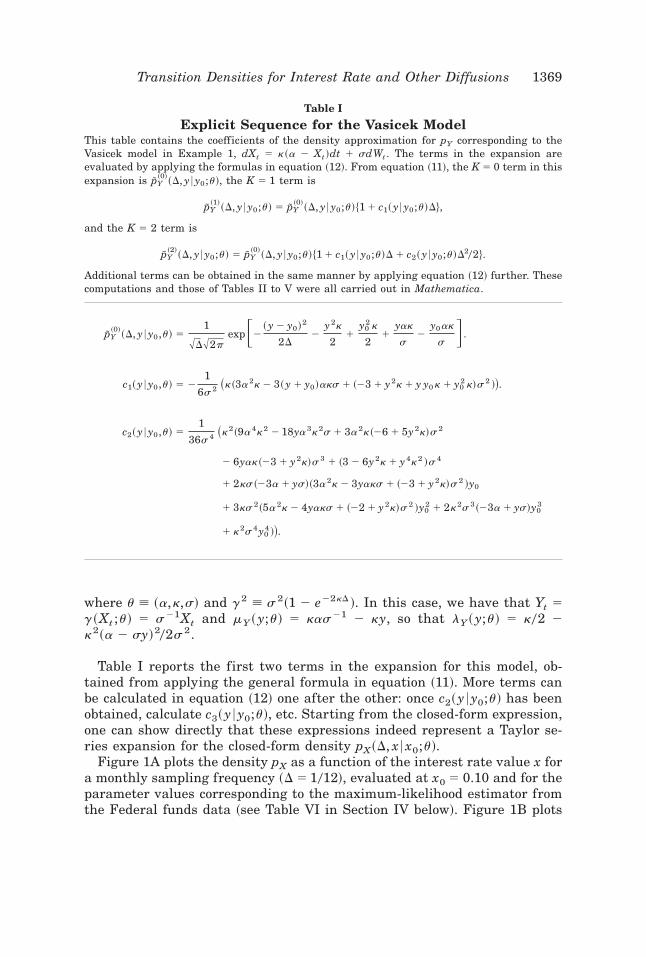
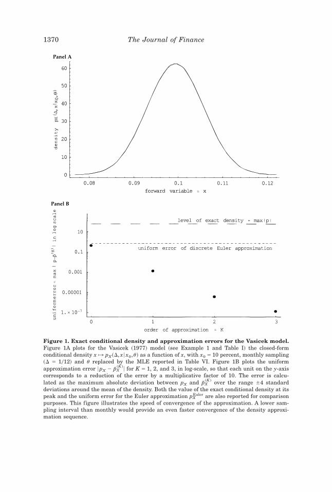
Figure 1A plots the density pX as a function of the interest rate value x fora monthly sampling frequency ~D 5 1012!, evaluated at x0 5 0.10 and for theparameter values corresponding to the maximum-likelihood estimator fromthe Federal funds data ~see Table VI in Section IV below!. Figure 1B plots

Table I

Explicit Sequence for the Vasicek ModelThis table contains the coefficients of the density approximation for pY corresponding to theVasicek model in Example 1, dXt 5 k~a 2 Xt!dt 1 sdWt . The terms in the expansion areevaluated by applying the formulas in equation ~12!. From equation ~11!, the K 5 0 term in thisexpansion is IpY

~0!~D, y 6y0;u!, the K 5 1 term is

IpY~1!

~D, y 6y0;u! 5 IpY~0!

~D, y 6y0;u!$1 1 c1~ y 6y0;u!D%,

and the K 5 2 term is

IpY~2!

~D, y 6y0;u! 5 IpY~0!

~D, y 6y0;u!$1 1 c1~ y 6y0;u!D 1 c2~ y 6y0;u!D202%.

Additional terms can be obtained in the same manner by applying equation ~12! further. Thesecomputations and those of Tables II to V were all carried out in Mathematica.

IpY~0!

~D, y 6y0,u! 51

%D%2pexpF2

~ y 2 y0!2

2D2

y2k

21

y02 k

21

yak

s2

y0 ak

sG.

c1~ y 6y0,u! 5 21

6s2 ~k~3a2k 2 3~ y 1 y0!aks 1 ~23 1 y2k 1 y y0 k 1 y02 k!s2 !!.

c2~ y 6y0,u! 51

36s4 ~k2~9a4k2 2 18ya3k2s 1 3a2k~26 1 5y2k!s2

2 6yak~23 1 y2k!s3 1 ~3 2 6y2k 1 y4k2 !s4

1 2ks~23a 1 ys!~3a2k 2 3yaks 1 ~23 1 y2k!s2 !y0

1 3ks2~5a2k 2 4yaks 1 ~22 1 y2k!s2 !y02 1 2k2s3~23a 1 ys!y0

3

1 k2s4y04 !!.


Panel A

Panel B

Figure 1. Exact conditional density and approximation errors for the Vasicek model.Figure 1A plots for the Vasicek ~1977! model ~see Example 1 and Table I! the closed-formconditional density x ° pX~D, x 6x0,u! as a function of x, with x0 5 10 percent, monthly sampling~D 5 1012! and u replaced by the MLE reported in Table VI. Figure 1B plots the uniformapproximation error 6pX 2 IpX

~K !6 for K 5 1, 2, and 3, in log-scale, so that each unit on the y-axiscorresponds to a reduction of the error by a multiplicative factor of 10. The error is calcu-lated as the maximum absolute deviation between pX and IpX

~K ! over the range 64 standarddeviations around the mean of the density. Both the value of the exact conditional density at itspeak and the uniform error for the Euler approximation pX

Euler are also reported for comparisonpurposes. This figure illustrates the speed of convergence of the approximation. A lower sam-pling interval than monthly would provide an even faster convergence of the density approxi-mation sequence.


the uniform approximation error 6pX 2 IpX~K !6 for K 5 1, 2, and 3, in log-scale.

The error is calculated as the maximum absolute deviation between pX andIpX~K ! over the range 64 standard deviations around the mean of the density,

and is also compared to the uniform error for the Euler approximation. Thestriking feature of the results is the speed of convergence to zero of theapproximation error as K goes from 1 to 2 and from 2 to 3. In effect, one canapproximate pX ~which is of order 1011 ! within 1023 with the first termalone ~K 5 1! and within 1027 with K 5 3, even though the interest rateprocess is only sampled once a month. Similar calculations for a weeklysampling frequency ~D 51052! reveal that the approximation error gets smallereven faster for this lower value of D.

In other words, small values of K already produce extremely precise ap-proximations to the true density, pX , and the approximation is even moreprecise if D is smaller. Of course, the exact density being Gaussian, in thiscase the expansion, whose leading term is Gaussian, has fairly little “work”to do to approximate the true density. In the Ornstein–Uhlenbeck case, theexpansion involves no correction for nonnormality, which is normally achievedthrough the change of variable X to Y; it reduces here to a linear transfor-mation and therefore does not change the nature of the leading term in theexpansion. Comparing the performance of the expansion to that of the Eulerapproximation in this model ~where both have the correct Gaussian form forthe density! reveals that the expansion is capable of correcting for the dis-cretization bias involved in a discrete approximation, whereas the Euler ap-proximation is limited to a first-order bias correction. In this case, the Eulerapproximation can be refined by increasing the precision of the conditionalmean and variance approximations ~see Huggins ~1997!!. Of course, discreteapproximations to equation ~1! of an order higher than equation ~15! areavailable, but they do not lead to explicit density approximations since, com-pared to the Euler equation ~15!, they involve combinations of multiple pow-ers of et1D ~see, e.g., Kloeden and Platen ~1992!!.

Example 2 (The CIR Model): Consider Feller’s ~1952! square-root specifi-cation

dXt 5 k~a 2 Xt !dt 1 s%Xt dWt , ~19!

proposed as a model for the short-term interest rate by Cox et al. ~1985!. Xis distributed on DX 5 ~0,1`! provided that q [ 2ka0s2 2 1 $ 0. Its tran-sition density is given by

pX ~D, x 6x0;u! 5 ce2u2v~v0u!q02Iq~2~uv!102 !, ~20!

with u [ ~a,k,s! all positive, c [ 2k0~s2$1 2 e2kD %!, u [ cx0e2kD, v [ cx, andIq is the modified Bessel function of the first kind of order q. Here Yt 5g~Xt ;u! 5 2%Xt 0s and mY~ y;u! 5 ~q 1 102!0y 2 ky02.


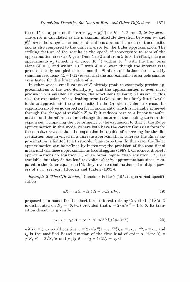
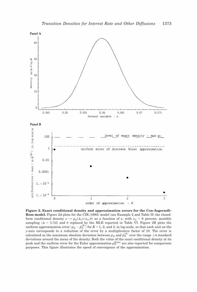
The first two terms in the explicit expansion are given in Table II. Whenevaluated at the maximum-likelihood estimates from Fed funds data, theresults reported in Figure 2 are very similar to those of Figure 1, again withan extremely fast convergence even for a monthly sampling frequency. Theuniform approximation error is reduced to 1025 with the first two terms,and 1028 with the first three terms included.

Example 3 (Inverse of Feller’s Square Root Model): In this example, I gen-erate densities for Ahn and Gao’s ~1998! specification of the interest rateprocess as one over an auxiliary process that follows a Cox–Ingersoll–Rossspecification. As a result of Itô’s Lemma, the model’s specification is

dXt 5 Xt ~k 2 ~s2 2 ka!Xt !dt 1 sXt302 dWt , ~21!

Table II

Explicit Sequence for the Cox–Ingersoll–Ross ModelThis table contains the coefficients of the density approximation for pY corresponding to theCox, Ingersoll, and Ross model in Example 2, dXt 5 k~a 2 Xt!dt 1 s%Xt dWt . The expansion forpY in this table applies also to the model proposed by Ahn and Gao ~1988! ~see Example 3!. Theterms in the expansion are evaluated by applying the formulas in equation ~12!. From equa-tion ~11!, the K 5 0 term in this expansion is IpY

~0!~D, y 6y0;u!, the K 5 1 term is

IpY~1!

~D, y 6y0;u! 5 IpY~0!

~D, y 6y0;u!$1 1 c1~ y 6y0;u!D%,


IpY~2!

~D, y 6y0;u! 5 IpY~0!

~D, y 6y0;u!$1 1 c1~ y 6y0;u!D 1 c2~ y 6y0;u!D202%.

Additional terms can be obtained in the same manner by applying equation ~12! further.

IpX~0!

~D, y 6y0,u! 51

%D%2pexpF2

~ y 2 y0!2

2D2

y2k

41

ky02

4 G y2~102!1~2ak0s 2 !y0~102!2~2ak0s2 ! .

c1~ y 6y0 u! 5 21

24yy0 s4 ~48a2k2 2 48aks2 1 9s4 1 yk2s2~224a 1 y2s2 !y0

1 y2k2s4y02 1 yk2s4y0

3 !.

c2~ y 6y0 u! 51

576y2y02 s8 ~9~256a4k4 2 512a3k3s2 1 224a2k2s4 1 32aks6 2 15s8 !

1 6yk2s2~224a 1 y2s2 !~16a2k2 2 16aks2 1 3s4 !y0

1 y2k2s4~672a2k2 2 48ak~2 1 y2k!s2 1 ~26 1 y4k2 !s4 !y02

1 2yk2s4~48a2k2 2 24ak~2 1 y2k!s2 1 ~9 1 y4k2 !s4 !y03

1 3y2k4s6~216a 1 y2s2 !y04 1 2y3k4s8y0

5 1 y2k4s8y06 !.


Panel A

Panel B

Figure 2. Exact conditional density and approximation errors for the Cox–Ingersoll–Ross model. Figure 2A plots for the CIR ~1985! model ~see Example 2 and Table II! the closed-form conditional density x ° pX~D, x 6x0,u! as a function of x, with x0 5 6 percent, monthlysampling ~D 5 1012! and u replaced by the MLE reported in Table VI. Figure 2B plots theuniform approximation error 6pX 2 IpX

~K !6 for K 5 1, 2, and 3, in log-scale, so that each unit on they-axis corresponds to a reduction of the error by a multiplicative factor of 10. The error iscalculated as the maximum absolute deviation between pX and IpX

~K ! over the range 64 standarddeviations around the mean of the density. Both the value of the exact conditional density at itspeak and the uniform error for the Euler approximation pX

Euler are also reported for comparisonpurposes. This figure illustrates the speed of convergence of the approximation.


Panel A

Panel B

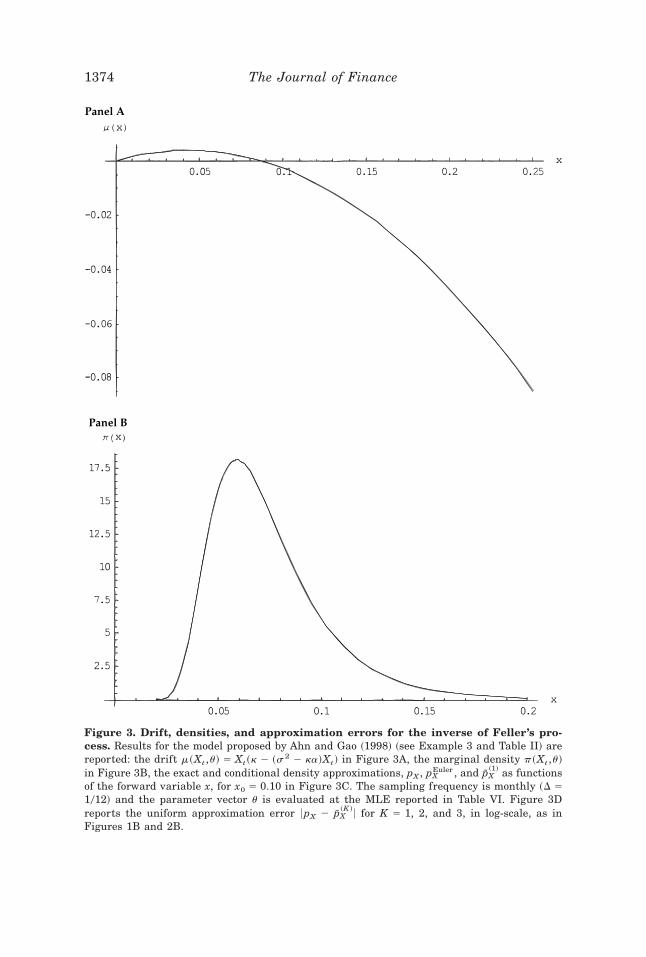
Figure 3. Drift, densities, and approximation errors for the inverse of Feller’s pro-cess. Results for the model proposed by Ahn and Gao ~1998! ~see Example 3 and Table II! arereported: the drift m~Xt ,u! 5 Xt~k 2 ~s2 2 ka!Xt! in Figure 3A, the marginal density p~Xt ,u!in Figure 3B, the exact and conditional density approximations, pX , pX

Euler , and IpX~1! as functions

of the forward variable x, for x0 5 0.10 in Figure 3C. The sampling frequency is monthly ~D 51012! and the parameter vector u is evaluated at the MLE reported in Table VI. Figure 3Dreports the uniform approximation error 6pX 2 IpX

~K !6 for K 5 1, 2, and 3, in log-scale, as inFigures 1B and 2B.


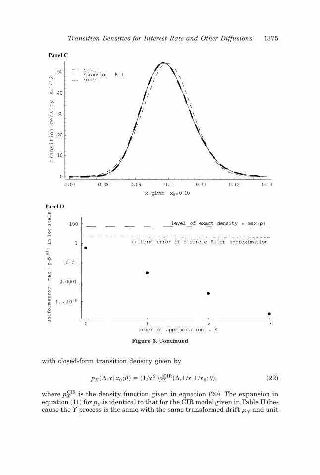
with closed-form transition density given by

pX ~D, x 6x0;u! 5 ~10x 2 !pXCIR~D,10x 610x0;u!, ~22!

where pXCIR is the density function given in equation ~20!. The expansion in

equation ~11! for pY is identical to that for the CIR model given in Table II ~be-cause the Y process is the same with the same transformed drift mY and unit

Panel C

Panel D

Figure 3. Continued


diffusion!. To get back to an expansion for X, the change of variable Y r X how-ever is different, and is now given by Yt 5 g~Xt ;u! 5 20~s%Xt!; hence the ex-pansion for pX will naturally be different from that for the CIR model ~it willnow approximate the left-hand side of equation ~22! rather than equation ~20!!.

Figure 3A reports the drift for this model, evaluated at the maximum-likelihood estimates from Table VI below. This model generates, in an envi-ronment where closed-form solutions are available, some of the effectsdocumented empirically by Aït-Sahalia ~1996b!: almost no drift while theinterest rate is in the middle of its range, strong mean-reversion when theinterest rate gets large. Figure 3B plots the unconditional or marginal den-sity, which is also the stationary density p~x,u! for this process when theinitial data point X0 has p as its distribution. p is given by

p~ y;u! [ expH2Ey

mY ~u;u! duJYEry

Sy

expH2EvmY ~u;u! duJ dv. ~23!

Figure 3C compares the exact conditional density in equation ~22!, its Eulerapproximation, and the expansion with K 5 1 for the conditioning interestrate x0 5 0.10. It is apparent from the figure that including the first termalone is sufficient to make the exact and approximate densities fall on top ofone another, whereas the Euler approximation is distinct. Finally, Figure 3Dreports the uniform approximation error between the Euler approximationand the exact density on the one hand, and between the first three terms inthe expansion and the exact density on the other. As can be seen from thesefigures, the expansion in equation ~11! provides again a very accurate ap-proximation to the exact density.

B. Density Approximation for Models with No Closed-Form Density

Of course, the usefulness of the method introduced in Aït-Sahalia ~1998! lieslargely in its ability to deliver explicit density approximations for models thatdo not have closed-form transition densities. The next two examples corre-spond to models recently proposed in the literature to describe the time seriesproperties of the short-term interest rate, and the final example illustrates theapplicability of the method to a double-well model where the stationary den-sity is bimodal.

Example 4 (Linear Drift, CEV Diffusion): Chan et al. ~1992! have pro-posed the specification

dXt 5 k~a 2 Xt ! dt 1 sXtr dWt , ~24!

with u [ ~a,k,s,r!. X is distributed on ~0,1`! when a . 0, k . 0, and r .102 ~if r 5 102; see Example 2 for an additional constraint!. This modeldoes not admit a closed-form density unless a 5 0 ~see Cox ~1996!!, which


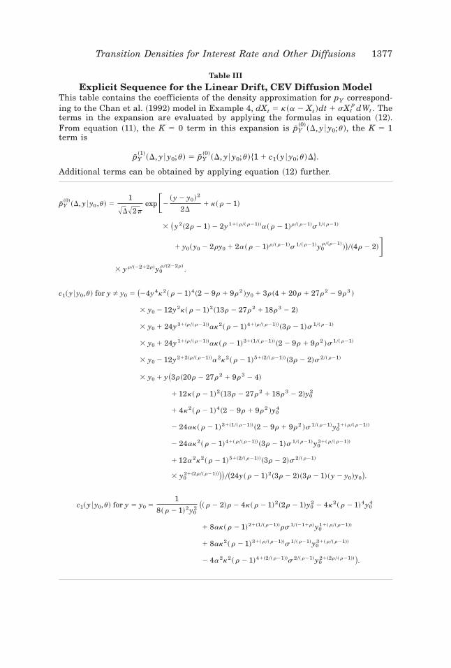
Table III

Explicit Sequence for the Linear Drift, CEV Diffusion ModelThis table contains the coefficients of the density approximation for pY correspond-ing to the Chan et al. ~1992! model in Example 4, dXt 5 k~a 2 Xt !dt 1 sXt

p dWt . Theterms in the expansion are evaluated by applying the formulas in equation ~12!.From equation ~11!, the K 5 0 term in this expansion is IpY

~0!~D, y 6y0;u!, the K 5 1

term is

IpY~1!

~D, y 6y0;u! 5 IpY~0!

~D, y 6y0;u!$1 1 c1~ y 6y0;u!D%.

Additional terms can be obtained by applying equation ~12! further.

IpY~0!

~D, y 6y0,u! 51

%D%2pexpF2

~ y 2 y0!2

2D1 k~ r 2 1!

3 ~ y2~2r 2 1! 2 2y11~ r0~ r21!!a~ r 2 1!r0~ r21!s10~ r21!

1 y0~ y0 2 2ry0 1 2a~ r 2 1!r0~ r21!s10~ r21!y0r0~r21!

!!0~4r 2 2!G3 yr0~2212r!y0

r0~222r! .

c1~ y 6y0,u! for y Þ y0 5 ~24y4k2~ r 2 1!4~2 2 9r 1 9r2 !y0 1 3r~4 1 20r 1 27r2 2 9r3 !

3 y0 2 12y2k~ r 2 1!2~13r 2 27r2 1 18r3 2 2!

3 y0 1 24y31~r0~ r21!!ak2~ r 2 1!41~r0~ r21!! ~3r 2 1!s10~ r21!

3 y0 1 24y11~r0~ r21!!ak~ r 2 1!31~10~ r21!! ~2 2 9r 1 9r2 !s10~ r21!

3 y0 2 12y212~r0~ r21!!a2k2~ r 2 1!51~20~ r21!! ~3r 2 2!s20~ r21!

3 y0 1 y~3r~20r 2 27r2 1 9r3 2 4!

1 12k~ r 2 1!2~13r 2 27r2 1 18r3 2 2!y02

1 4k2~ r 2 1!4~2 2 9r 1 9r2 !y04

2 24ak~ r 2 1!31~10~ r21!! ~2 2 9r 1 9r2 !s10~ r21!y011~ r0~ r21!!

2 24ak2~ r 2 1!41~ r0~ r21!! ~3r 2 1!s10~ r21!y031~ r0~ r21!!

1 12a2k2~ r 2 1!51~20~ r21!! ~3r 2 2!s20~ r21!

3 y021~2r0~ r21!!!!0~24y~ r 2 1!2~3r 2 2!~3r 2 1!~ y 2 y0!y0!.

c1~ y 6y0,u! for y 5 y0 51

8~ r 2 1!2y02 ~~ r 2 2!r 2 4k~ r 2 1!2~2r 2 1!y0

2 2 4k2~ r 2 1!4y04

1 8ak~ r 2 1!21~10~ r21!!rs10~211r!y011~ r0~ r21!!

1 8ak2~ r 2 1!31~ r0~ r21!!s10~ r21!y031~ r0~ r21!!

2 4a2k2~ r 2 1!41~20~ r21!!s20~ r21!y021~2r0~ r21!! !.


then makes it unrealistic for interest rates. I will concentrate on the casewhere r . 1, which corresponds to the empirically plausible estimate forU.S. interest rate data. The transformation from X to Y is given by Yt 5g~Xt ;u! 5 Xt

12r 0$s~ r 2 1!% and

Panel A

Panel B

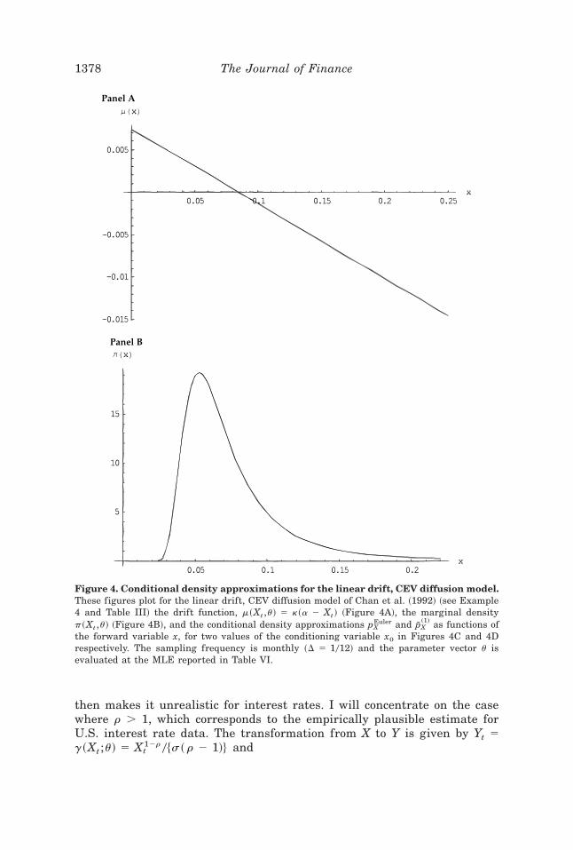
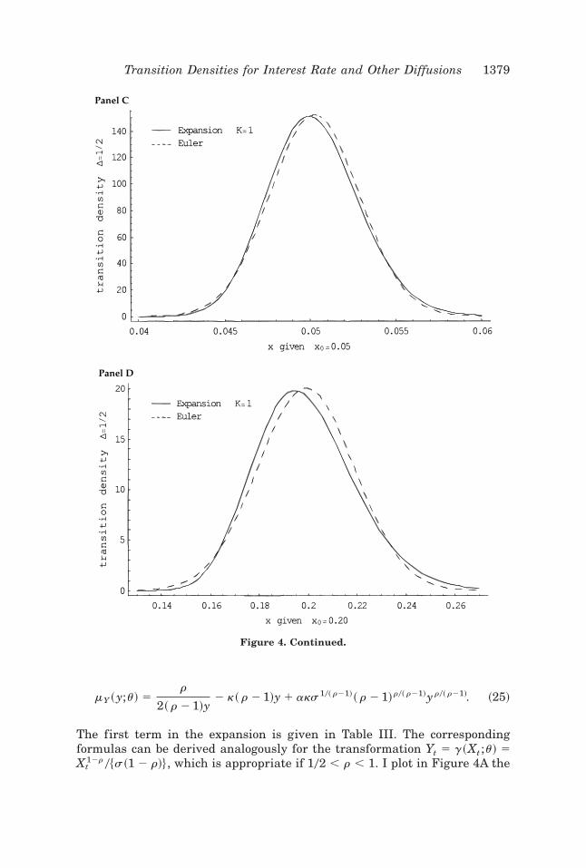
Figure 4. Conditional density approximations for the linear drift, CEV diffusion model.These figures plot for the linear drift, CEV diffusion model of Chan et al. ~1992! ~see Example4 and Table III! the drift function, m~Xt ,u! 5 k~a 2 Xt! ~Figure 4A!, the marginal densityp~Xt ,u! ~Figure 4B!, and the conditional density approximations pX

Euler and IpX~1! as functions of

the forward variable x, for two values of the conditioning variable x0 in Figures 4C and 4Drespectively. The sampling frequency is monthly ~D 5 1012! and the parameter vector u isevaluated at the MLE reported in Table VI.


mY ~ y;u! 5r

2~ r 2 1!y2 k~ r 2 1!y 1 aks10~ r21! ~ r 2 1!r0~ r21!yr0~ r21!. ~25!

The first term in the expansion is given in Table III. The correspondingformulas can be derived analogously for the transformation Yt 5 g~Xt ;u! 5Xt

12r 0$s~1 2 r!% , which is appropriate if 102 , r , 1. I plot in Figure 4A the

Panel C

Panel D

Figure 4. Continued.


drift function corresponding to maximum-likelihood estimates ~based on theexpansion with K 5 1, see Table VI below!, in Figure 4B I plot the uncondi-tional density, and in Figures 4C and 4D the conditional density approxima-tions for monthly sampling at x0 5 0.05 and 0.20, respectively.

Example 5 (Nonlinear Mean Reversion): The following model was de-signed to produce very little mean reversion while interest rate values re-main in the middle part of their domain, and strong nonlinear mean reversionat either end of the domain ~see Aït-Sahalia ~1996b!!:

dXt 5 ~a21 Xt21 1 a0 1 a1 Xt 1 a2 Xt

2 ! dt 1 sXtr dWt , ~26!

with u [ ~a21,a0,a1,a2,s,r!. This model has been estimated empirically byAït-Sahalia ~1996b!, Conley et al. ~1997!, and Gallant and Tauchen ~1998!using a variety of empirical techniques. The new method in this paper makesit possible to estimate it using maximum likelihood. I again concentrate onthe case where r . 1, and to save space I evaluate the formulas in Table IVfor r 5 302. This process has DX 5 ~0,1`!, Yt 5 g~Xt ;u! 5 20~s%Xt!, and

mY ~ y;u! 5302 2 2a2 0s2

y2

a1 y

22

a0 s2y3

82

a21 s4y5

32. ~27!

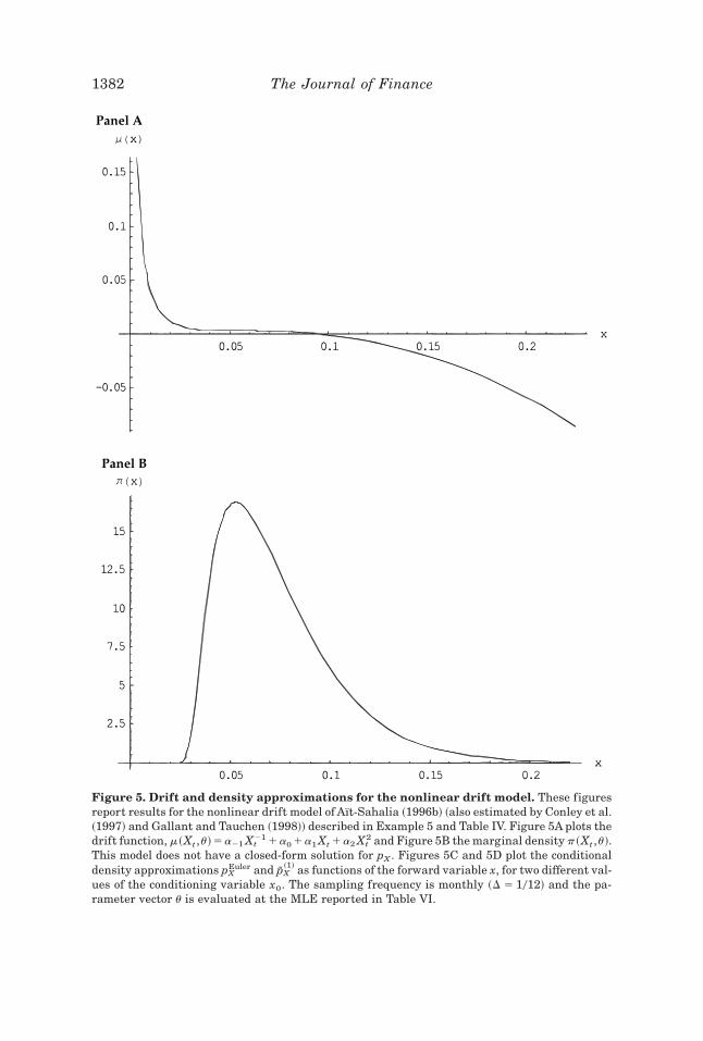
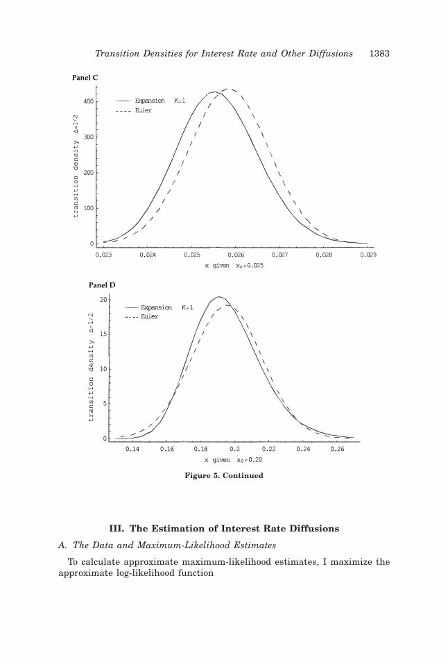
Figure 5A plots the drift evaluated at the maximum-likelihood parameterestimates ~corresponding to K 5 1!. Figure 5B plots the unconditional ormarginal density of the process: in the specification test in Aït-Sahalia ~1996b!,this density is matched against a nonparametric kernel estimator. Fig-ures 5C and 5D contain the conditional density approximations for K 5 1,compared with the Euler approximation, for the two values x0 5 0.025 and0.20, respectively. As before, sampling is at the monthly frequency.

Example 6 (Double-Well Potential): In this example, I generate a bimodalstationary density through the specification

dXt 5 ~Xt 2 Xt3 ! dt 1 dWt . ~28!

This model is distributed on DX 5 ~2`,1`!. Since the model is already setin unit diffusion, no transformation is needed ~Y 5 X !.

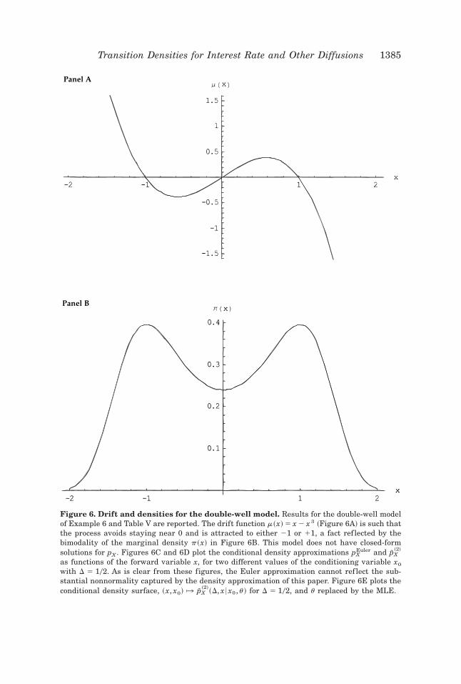
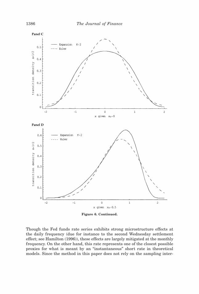
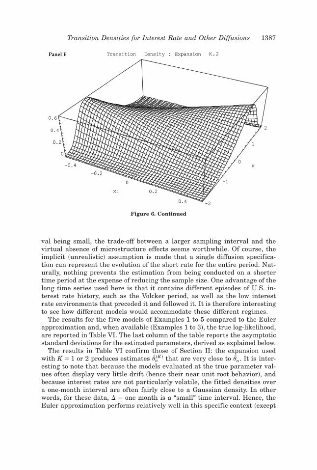
Table V contains the first two terms of the expansion; Figure 6A plots itsdrift, Figure 6B its marginal density, and Figures 6C and 6D the transitiondensity for K 5 2, monthly sampling, and x0 5 0.0 and 0.5, respectively, withD 5 102. As is apparent from the figures, the densities in this model exhibitstrong nonnormality, which obviously cannot be captured by the Euler ap-proximation of equation ~16!.


Table IV

Explicit Sequence for the Nonlinear Drift ModelThis table contains the coefficients of the density approximation for pY corresponding to themodel in Aït-Sahalia ~1996b!, Conley et al. ~1997!, and Tauchen ~1997! given in Example 5,dXt 5 ~a21 Xt

21 1 a0 1 a1 Xt 1 a2 Xt2 ! dt 1 sXt

r dWt with r 5 302. The terms in the expansion areevaluated by applying the formulas in equation ~12!. From equation ~11!, the K 5 0 term in thisexpansion is IpY

~0!~D, y 6y0;u! and the K 5 1 term is

IpY~1!

~D, y 6y0;u! 5 IpY~0!

~D, y 6y0;u!$1 1 c1~ y 6y0;u!D%.

Additional terms can be obtained by applying equation ~12! further.

IpX~0!

~D,y 6y0,u! 51

%D%2pexpF2

~ y 2 y0!2

2D1

1

192~s4~2y6 1 y0

6 !a21

2 6~ y2 2 y02 !~s2~ y2 1 y0

2 !a0 1 8a1!!G3 y ~302!2~2a20s2 !y0

2~302!1~2a20s2 !.

c1~ y 6y0 u! 5 21

7096320ys4y0~315ys12y0~ y10 1 y9y0 1 y8y0

2 1 y7y03 1 y6y0

4 1 y5y05 1 y4y0

6

1 y3y07 1 y2y0

8 1 yy09 1 y0

10 !a212 1 88ys6y0 a21

3 ~35s4~ y8 1 y7y0 1 y6y02 1 y5y0

3 1 y4y04 1 y3y0

5

1 y2y06 1 yy0

7 1 y08 !

3 a0 1 36~256y4s2 2 56y3s2y0 2 56y2s2y02 2 56ys2y0

3

2 56s2y04 1 5y6s2a1 1 5y5s2y0 a1 1 5y4s2y0

2 a1

1 5y3s2y03 a1 1 5y2s2y0

4 a1 1 5ys2y05 a1

1 5s2y06 a1 1 28y4a2 1 28y3y0 a2 1 28y2y0

2 a2

1 28yy03 a2 1 28y0

4 a2!!

1 528~15ys8y0~ y6 1 y5y0 1 y4y02 1 y3y0

3 1 y2y04 1 yy0

5 1 y06 !

3 a02 1 56ys4y0 a0~230y2s2 2 30ys2y0 2 30s2y0

2

1 3y4s2a1 1 3y3s2y0 a1

1 3y2s2y02 a1 1 3ys2y0

3 a1 1 3s2y04 a1

1 20y2a2 1 20yy0 a2 1 20y02 a2!

1 560~9s4 2 24ys4y0 a1 1 y3s4y0 a12 1 y2s4y0

2 a12

1 ys4y03 a1

2 2 48s2a2 1 24ys2y0 a1 a2 1 48a22 !!!.


Panel A

Panel B

Figure 5. Drift and density approximations for the nonlinear drift model. These figuresreport results for the nonlinear drift model of Aït-Sahalia ~1996b! ~also estimated by Conley et al.~1997! and Gallant and Tauchen ~1998!! described in Example 5 and Table IV. Figure 5A plots thedrift function, m~Xt ,u! 5 a21 Xt

21 1 a0 1 a1 Xt 1 a2 Xt2 and Figure 5B the marginal density p~Xt ,u!.

This model does not have a closed-form solution for pX . Figures 5C and 5D plot the conditionaldensity approximations pX

Euler and IpX~1! as functions of the forward variable x, for two different val-

ues of the conditioning variable x0. The sampling frequency is monthly ~D 5 1012! and the pa-rameter vector u is evaluated at the MLE reported in Table VI.


III. The Estimation of Interest Rate Diffusions

A. The Data and Maximum-Likelihood Estimates

To calculate approximate maximum-likelihood estimates, I maximize theapproximate log-likelihood function

Panel C

Panel D

Figure 5. Continued


,n~K ! ~u! [ n21 (

i51

n

ln$ IpX~K !

~D, XiD 6X~i21!D ;u!% ~29!

~with the convention that ln~a! 5 2` if a , 0! over u in Q. This results inan estimator Zun

~K ! , which, as shown in Aït-Sahalia ~1998!, is close to the exact~but uncomputable in practice! maximum-likelihood estimator Zun.

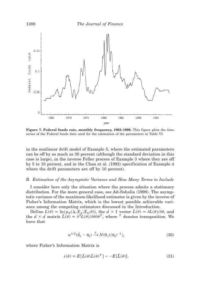
The data consist of monthly sampling of the Fed funds rate between Jan-uary 1963 and December 1998 ~see Figure 7!. The source for the data is theH-15 Federal Reserve Statistical Release ~Selected Interest Rate Series!.

Table V

Explicit Sequence for the Double-Well ModelThis table contains the coefficients of the density approximation for pY corresponding to themodel in Example 6, dXt 5 ~Xt 2 Xt

3 ! dt 1 dWt . The terms in the expansion are evaluated byapplying the formulas in equation ~12!. From equation ~11!, the K 5 0 term in this expansion isIpY~0!

~D, y 6y0;u!, the K 5 1 term is

IpY~1!

~D, y 6y0;u! 5 IpY~0!

~D, y 6y0;u!$1 1 c1~ y 6y0;u!D%,


IpY~2!

~D, y 6y0;u! 5 IpY~0!

~D, y 6y0;u!$1 1 c1~ y 6y0;u!D 1 c2~ y 6y0;u!D202%.

Additional terms can be obtained in the same manner by applying equation ~12! further.

IpX~0!

~D, y 6y0,u! 51

%D%2pexpF2

~ y 2 y0!2

2D1

y2

22

y4

42

y02

21

y04

4 G.

c1~ y 6y0,u! 51

210~2105 1 70y2 1 42y4 2 15y6 1 ~70y 1 42y3 2 15y5 !y0 1 ~70 1 42y2 2 15y4 !y0

2

1 ~42y 2 15y3 !y03 1 ~42 2 15y2 !y0

4 2 15yy05 2 15y0

6 !.

c2~ y 6y0,u! 51

44100~25725 1 11760y2 2 19670y4 1 9030y6 2 336y8 2 1260y10 1 225y12

1 2y~10290 2 12110y2 1 7455y4 2 336y6 2 1260y8 1 225y10 !y0

1 3~3920 2 7490y2 1 6930y4 2 336y6 2 1260y8 1 225y10 !y02

1 2y~212110 1 10395y2 1 378y4 2 2520y6 1 450y8 !y03

1 5~23934 1 4158y2 1 504y4 2 1260y6 1 225y8 !y04

1 6y~2485 1 126y2 2 1050y4 1 225y6 !y05

1 21~430 2 48y2 2 300y4 1 75y6 !y06 1 6y~2112 2 840y2 1 225y4 !y0

7

1 3~2112 2 1260y2 1 375y4 !y08 1 180y~214 1 5y2 !y0

9

1 45~228 1 15y2 !y010 1 450yy0

11 1 225y012 !.


Panel A

Panel B

Figure 6. Drift and densities for the double-well model. Results for the double-well modelof Example 6 and Table V are reported. The drift function m~x! 5 x 2 x 3 ~Figure 6A! is such thatthe process avoids staying near 0 and is attracted to either 21 or 11, a fact ref lected by thebimodality of the marginal density p~x! in Figure 6B. This model does not have closed-formsolutions for pX . Figures 6C and 6D plot the conditional density approximations pX

Euler and IpX~2!

as functions of the forward variable x, for two different values of the conditioning variable x0

with D 5 102. As is clear from these figures, the Euler approximation cannot ref lect the sub-stantial nonnormality captured by the density approximation of this paper. Figure 6E plots theconditional density surface, ~x, x0! ° IpX

~2!~D, x 6x0, u! for D 5 102, and u replaced by the MLE.


Though the Fed funds rate series exhibits strong microstructure effects atthe daily frequency ~due for instance to the second Wednesday settlementeffect; see Hamilton ~1996!!, these effects are largely mitigated at the monthlyfrequency. On the other hand, this rate represents one of the closest possibleproxies for what is meant by an “instantaneous” short rate in theoreticalmodels. Since the method in this paper does not rely on the sampling inter-

Panel C

Panel D

Figure 6. Continued.


val being small, the trade-off between a larger sampling interval and thevirtual absence of microstructure effects seems worthwhile. Of course, theimplicit ~unrealistic! assumption is made that a single diffusion specifica-tion can represent the evolution of the short rate for the entire period. Nat-urally, nothing prevents the estimation from being conducted on a shortertime period at the expense of reducing the sample size. One advantage of thelong time series used here is that it contains different episodes of U.S. in-terest rate history, such as the Volcker period, as well as the low interestrate environments that preceded it and followed it. It is therefore interestingto see how different models would accommodate these different regimes.

The results for the five models of Examples 1 to 5 compared to the Eulerapproximation and, when available ~Examples 1 to 3!, the true log-likelihood,are reported in Table VI. The last column of the table reports the asymptoticstandard deviations for the estimated parameters, derived as explained below.

The results in Table VI confirm those of Section II: the expansion usedwith K 5 1 or 2 produces estimates Zun

~K ! that are very close to Zun. It is inter-esting to note that because the models evaluated at the true parameter val-ues often display very little drift ~hence their near unit root behavior!, andbecause interest rates are not particularly volatile, the fitted densities overa one-month interval are often fairly close to a Gaussian density. In otherwords, for these data, D 5 one month is a “small” time interval. Hence, theEuler approximation performs relatively well in this specific context ~except

Panel E

Figure 6. Continued


in the nonlinear drift model of Example 5, where the estimated parameterscan be off by as much as 30 percent ~although the standard deviation in thiscase is large!, in the inverse Feller process of Example 3 where they are offby 5 to 10 percent, and in the Chan et al. ~1992! specification of Example 4where the drift parameters are off by 10 percent!.

B. Estimation of the Asymptotic Variance and How Many Terms to Include

I consider here only the situation where the process admits a stationarydistribution. For the more general case, see Aït-Sahalia ~1998!. The asymp-totic variance of the maximum-likelihood estimator is given by the inverse ofFisher’s Information Matrix, which is the lowest possible achievable vari-ance among the competing estimators discussed in the Introduction.

Define L~u! [ ln~ pX~D, XD6X0;u!!, the d 3 1 vector L̂~u! [ ?L~u!0?u, andthe d 3 d matrix ^L̂~u! [ ?2L~u!0?u?uT, where T denotes transposition. Wehave that

n102~ Zun 2 u0!d&& N~0, i ~u0!21 !, ~30!

where Fisher’s Information Matrix is

i ~u! [ E @L̂~u!L̂~u!T # 5 2E @ ^L̂~u!# . ~31!

Figure 7. Federal funds rate, monthly frequency, 1963–1998. This figure plots the timeseries of the Federal funds data used for the estimation of the parameters in Table VI.


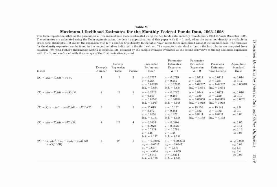
Table VI

Maximum-Likelihood Estimates for the Monthly Federal Funds Data, 1963–1998This table reports the MLE for the parameters of five interest rate models estimated using the Fed funds data, monthly from January 1963 through December 1998.The estimates are calculated using the Euler approximation, the density approximation of this paper with K 5 1, and, when the transition density is available inclosed-form ~Examples 1, 2 and 3!, the expansion with K 5 2 and the true density. In the table, “ln L” refers to the maximized value of the log-likelihood. The formulasfor the density expansion can be found in the respective tables indicated in the third column. The asymptotic standard errors in the last column are computed fromequation ~30!, with Fisher’s Information Matrix in equation ~31! replaced by the sample averages evaluated at the second derivative of the log-likelihood expansionwith K 5 1, and confirmed with the average of the first derivative squared.

ModelExampleNumber

DensityExpansion

Table Figure

ParameterEstimates:

Euler

ParameterEstimates:Expansion

K 5 1

ParameterEstimates:Expansion

K 5 2

ParameterEstimates:

True Density

AsymptoticStandard

Error

dXt 5 k~a 2 Xt ! dt 1 sdWt 1 I 1 a 5 0.0717 a 5 0.0719 a 5 0.0717 a 5 0.0717 a: 0.014k 5 0.258 k 5 0.257 k 5 0.261 k 5 0.261 k: 0.12s 5 0.02213 s 5 0.02237 s 5 0.02237 s 5 0.02237 s: 0.00078ln L 5 3.634 ln L 5 3.634 ln L 5 3.634 ln L 5 3.634

dXt 5 k~a 2 Xt ! dt 1 s%Xt dWt 2 II 2 a 5 0.0732 a 5 0.0742 a 5 0.0742 a 5 0.0721 a: 0.016k 5 0.145 k 5 0.189 k 5 0.189 k 5 0.219 k: 0.10s 5 0.06521 s 5 0.06658 s 5 0.06658 s 5 0.06665 s: 0.0023ln L 5 3.917 ln L 5 3.918 ln L 5 3.918 ln L 5 3.918

dXt 5 Xt~k 2 ~s2 2 ka!Xt ! dt 1 sXt302 dWt 3 II 3 a 5 15.019 a 5 15.157 a 5 15.150 a 5 15.141 a: 2.9

k 5 0.177 k 5 0.181 k 5 0.182 k 5 0.182 k: 0.1s 5 0.8059 s 5 0.8211 s 5 0.8211 s 5 0.8211 s: 0.03ln L 5 4.171 ln L 5 4.158 ln L 5 4.158 ln L 5 4.158

dXt 5 k~a 2 Xt ! dt 1 sXtr dWt 4 III 4 a 5 0.0808 a 5 0.0844 a: 0.05

k 5 0.0972 k 5 0.0876 k: 0.11s 5 0.7224 s 5 0.7791 s: 0.16r 5 1.46 r 5 1.48 r: 0.08ln L 5 4.172 ln L 5 4.159

dXt 5 ~a21 Xt21 1 a0 1 a1 Xt 1 a2 Xt

2 ! dt 5 IV 5 a21 5 0.00107 a21 5 0.000693 a21: 0.0021 sXt

302 dWt a0 5 20.0517 a0 5 20.0347 a0: 0.09a1 5 0.877 a1 5 0.676 a1: 1.3a2 5 24.604 a2 5 24.059 a2: 6.4s 5 0.8047 s 5 0.8214 s: 0.03ln L 5 4.173 ln L 5 4.160

Tran

sitionD

ensities

forIn

terestR

atean

dO

ther

Diffu

sions

1389

Note that it is necessary that the transition function pX not be uniformlyf lat in the direction of any one of the parameters um, m 5 1, . . . ,d, otherwise?pX~D, x 6x0;u!0?um [ 0 for all ~x, x0! and the model cannot be identified. Inother words, no parameter entering the likelihood function can be redun-dant. The asymptotic standard deviations from equation ~30! are reported inthe last column of Table VI for the interest rate models estimated above,with the expected values in equation ~31! replaced by the sample averagesevaluated at the MLE.

Test statistics can be derived. Suppose that the model is given by equa-tion ~1! and that we wish to test H0 : u 5 u0 against the two-sided alternativeHa : u Þ u0. The likelihood ratio test statistic evaluated behaves under H0 as:

2$,n~ Zun! 2 ,n~u0!%d&&xd

2 . ~32!

Distributional results can also be obtained for tests of a nested model thatonly allows for Nd free parameters from the d parameters in u, and one canalso consider Rao’s efficient score statistic, which depends only on the re-stricted estimator Nun, and Wald’s test statistic, which depends only on theunrestricted estimator Zun.

In all the results above, one can then replace Zun ~respectively Nun! by Zun~K !

~respectively Nun~K ! !. As the examples above have shown, it is not necessary to

go much beyond K 5 2 in the relevant financial examples to estimate thetrue density with a high degree of precision. More generally, to select anappropriate K at which to stop adding terms to the expansion, the followingapproach can be adopted: take K large enough so that the approximationerror made in replacing pX by IpX

~K ! is smaller than the sampling error due tothe random character of the data, by a predetermined factor.

That is, in

66 Zun~K ! 2 u0 66 # 66 Zun

~K ! 2 Zun 661 66 Zun 2 u0 66 ~33!

we can estimate the asymptotic standard variance of Zun about u0 by equation~30!. By Chebyshev’s Inequality, one can then bound the second term on theright-hand-side of equation ~33!. We can then stop considering higher orderapproximations at an order K such that the distance between the two suc-cessive estimates Zun

~K ! and Zun~K21! is an order of magnitude smaller than the

distance between Zun and u0. In practice, this is unlikely to make much of adifference and in most cases one can safely restrict attention to the first twoterms, K 5 1 and K 5 2.

IV. Conclusion

This paper has demonstrated how to obtain very accurate closed-form ap-proximations to the respective transition densities of a variety of modelscommonly used to represent the dynamics of the short-term interest rate.


Applications to derivative pricing, consisting of obtaining pricing formulasfor any underlying price process, have been brief ly outlined and will bedeveloped in future work. Finally, an extension of these results to multivar-iate diffusions will be investigated.

Appendix: Regularity Conditions

ASSUMPTION 1 ~Smoothness of the coefficients!: The functions m~x;u! and s~x;u!are infinitely differentiable in x in DX, and twice continuously differentiablein u in the parameter space Q , Rd.

ASSUMPTION 2 ~Nondegeneracy of the diffusion!:

1. If DX 5 ~2`,1`!, there exists a constant c such that s~x;u! . c . 0 forall x [ DX and u [ Q.

2. If DX 5 ~0,1`!, I allow for the possible local degeneracy of s at x 5 0:If s~0;u! 5 0, then there exist constants j0 , v $ 0, r $ 0 such thats~x;u! $ vxr for all 0 , x , j0 and u [ Q. Away from 0, s is nonde-generate; that is, for each j . 0, there exists a constant cj such thats~x;u! $ cj . 0 for all x [ @j 1`! and u [ Q.

Assumption 3 below restricts the behavior of the function mY and its de-rivatives near the boundaries of DY . It is formulated in terms of the functionmY for reasons of convenience, but the equivalent formulation directly interms of the original functions m and s can be obtained from equation ~8!.Recall that lY~ y;u! [ 2~mY

2 ~ y;u! 1 ?mY~ y;u!0?y!02.

ASSUMPTION 3 ~Boundary behavior!: For all u [ Q, mY~ y;u!, ?mY~ y;u!0?y, and?2mY ~ y;u!0?y2 have at most exponential growth near the infinity boundariesand limyr ry or Sy lY ~ y;u! , 1`.

1. Left Boundary:i. If ry 5 01, there exist constants e0 , k, a such that for all 0 , y # e0

and u [ Q,mY~ y;u! $ ky2a where either a . 1 and k . 0, or a 5 1and k $ 1.

ii. If ry 5 2`, there exist constants E0 . 0 and K . 0 such that for ally # 2E0 and u [ Q,mY~ y;u! $ Ky.

2. Right Boundary: If Sy 5 1`, there exist constants E0 . 0 and K . 0such that for all y $ E0 and u [ Q,mY~ y;u! # Ky.

The following remarks can help demonstrate the generality of these as-sumptions:

1. The upper bound limyr ry or Sy lY ~ y;u! , 1` does not restrict lY fromgoing to 2` near the boundaries.

2. Similarly, Assumption 3 does not preclude mY from going to 2` veryfast near Sy, and similarly, from going to 1` very fast near ry. Assump-tion 3 only restricts how large mY can grow if it has the “wrong” sign;


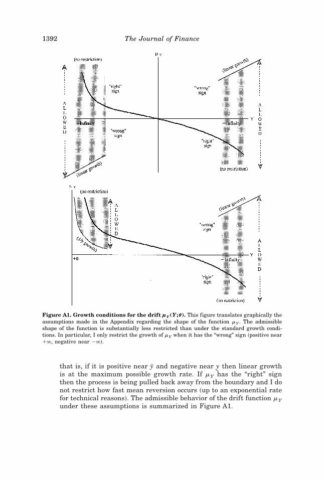
that is, if it is positive near Sy and negative near ry then linear growthis at the maximum possible growth rate. If mY has the “right” signthen the process is being pulled back away from the boundary and I donot restrict how fast mean reversion occurs ~up to an exponential ratefor technical reasons!. The admissible behavior of the drift function mYunder these assumptions is summarized in Figure A1.

Figure A1. Growth conditions for the drift µY(Y ;u). This figure translates graphically theassumptions made in the Appendix regarding the shape of the function mY . The admissibleshape of the function is substantially less restricted than under the standard growth condi-tions. In particular, I only restrict the growth of mY when it has the “wrong” sign ~positive near1`, negative near 2`!.


3. The constraints on the behavior of the function mY are essentially thebest possible. For example, if mY has the “wrong” sign near an infinityboundary, and grows faster than linearly, then Y explodes in finitetime. Near a zero boundary at 01, if there exist k . 0 and a , 1 suchthat mY~ y;u! # ky2a in a neighborhood of 01 then 0 and negative val-ues become attainable.

4. I can now fully characterize the boundary behavior of the diffusion Yimplied by the assumptions made: if 1` is a boundary then it is nat-ural if, near 1`, 6mY~ y;u!6 # Ky and entrance if mY~ y;u! # 2Ky b forsome b . 1. If 2` is a boundary then it is natural if, near 2`,6mY~ y;u!6 # K 6y 6 and entrance if mY~ y;0! $ K 6y 6b for some b . 1. If 01

is a boundary, then it is entrance.Both entrance and natural boundaries are unattainable ~see Feller

~1952! or Karlin and Taylor ~1981, Sec. 15.6! for the definition of bound-aries!. Natural boundaries can neither be reached in finite time, norcan the diffusion be started from there. Entrance boundaries, such as01, cannot be reached starting from an interior point in DY 5 ~0,1`!,but it is possible for Y to begin there. In that case, the process movesquickly away from 0 and never returns there. Typically, economic in-tuition says little about how the process would behave if it were tostart at the boundary, or whether that is even possible, and hence it issensible to allow both types of boundary behavior.

5. Assumption 3 neither requires nor implies that the process is station-ary. When both boundaries of the domain DY are entrance boundariesthen the process is necessarily stationary with unconditional ~margin-al! density,

p~ y;u! [ expH2Ey

mY ~u;u! duJYEry

Sy

expH2EvmY ~u;u! duJ dv,

~A.1!

provided that the initial random variable Y0 is itself distributed withthe same density p. When at least one of the boundaries is natural,stationarity is neither precluded nor implied. For instance, both anOrnstein–Uhlenbeck process, where mY~ y;u! 5 k~a 2 y!, and a stan-dard Brownian motion, where mY~ y;u! 5 0, satisfy the assumptionsmade, and both have natural boundaries at 2` and 1`. Yet the for-mer process is stationary, due to mean reversion, while the latter ~nullrecurrent! is not.

Finally, the following assumption is needed for the purpose of maximizingthe log-likelihood function only, not for the purpose of constructing the den-sity expansion in equation ~11!.


ASSUMPTION 4 ~Strengthening of Assumption 2 in the limiting case wherea 5 1 and the diffusion is degenerate at 0!: Recall the constant r in As-sumption 2(2), and the constants a and k in Assumption 3(1.i). If a 5 1,then either r $ 1 with no restriction on k, or k $ 2r0~1 2 r! if 0 , r , 1.If a . 1, no restriction is required.

REFERENCES

Ahn, Dong-Hyun, and Bin Gao, 1998, A parametric nonlinear model of term structure dynam-ics, Working paper, University of North Carolina at Chapel Hill.

Aït-Sahalia, Yacine, 1996a, Nonparametric pricing of interest rate derivative securities, Econ-ometrica 64, 527–560.

Aït-Sahalia, Yacine, 1996b, Testing continuous-time models of the spot interest rate, Review ofFinancial Studies 9, 385–426.

Aït-Sahalia, Yacine, 1998, Maximum-likelihood estimation of discretely sampled diffusions: Aclosed-form approach, Working paper, Princeton University.

Bibby, Bo M., and Michael Sørenson, 1995, Martingale estimation functions for discretely ob-served diffusion processes, Bernoulli 1, 17–39.

Black, Fisher, and Myron Scholes, 1973, The pricing of options and corporate liabilities, Jour-nal of Political Economy 81, 637–654.

Chan, K. C., G. Andrew Karolyi, Francis A. Longstaff, and Anthony B. Sanders, 1992, An em-pirical comparison of alternative models of the short-term interest rate, Journal of Finance47, 1209–1227.

Conley, Timothy G., Lars P. Hansen, Erzo G. J. Luttmer, and José A. Scheinkman, 1997, Short-term interest rates as subordinated diffusions, Review of Financial Studies 10, 525–578.

Cox, John C., 1996, The constant elasticity of variance option pricing model, The Journal ofPortfolio Management, Special issue.

Cox, John C., John E. Ingersoll, and Stephen A. Ross, 1985, A theory of the term structure ofinterest rates, Econometrica 53, 385–407.

Cox, John C., and Stephen A. Ross, 1976, The valuation of options for alternative stochasticprocesses, Journal of Financial Economics 3, 145–166.

Dacunha-Castelle, Didier, and Danielle Florens-Zmioru, 1986, Estimation of the coefficients ofa diffusion from discrete observations, Stochastics 19, 263–284.

Duffie, Darrell, and Peter Glynn, 1997, Estimation of continuous-time Markov processes sam-pled at random time intervals, Working paper, Stanford University.

Duffie, Darrell, and Kenneth Singleton, 1993, Simulated moments estimation of Markov mod-els of asset prices, Econometrica 61, 929–952.

Elerian, Ola, Sidartha Chib, and Neil Shephard, 1998, Likelihood inference for discretely ob-served non-linear diffusions, Working paper, Oxford University.

Eraker, Bjorn, 1997, MCMC analysis of diffusion models with application to finance, Workingpaper, Norwegian School of Economics, Bergen.

Feller, William, 1952, The parabolic differential equations and the associated semi-groups oftransformations, Annals of Mathematics 55, 468–519.

Florens, Jean-Pierre, Eric Renault, and Nizar Touzi, 1995, Testing for embeddability by sta-tionary scalar diffusions, Econometric Theory, forthcoming.

Gallant, A. Ronald, and George Tauchen, 1998, Reprojecting partially observed systems with anapplication to interest rate diffusions, Journal of the American Statistical Association 93,10–24.

Gihman, I. I., and A. V. Skorohod, 1972, Stochastic Differential Equations ~Springer-Verlag,New York!.

Gouriéroux, Christian, Alain Monfort, and Eric Renault, 1993, Indirect inference, Journal ofApplied Econometrics 8, S85–S118.

Hamilton, James D, 1996, The daily market for Federal funds, Journal of Political Economy104, 26–56.


Hansen, Lars P., and José A. Scheinkman, 1995, Back to the future: Generating moment im-plications for continuous time Markov processes, Econometrica 63, 767–804.

Hansen, Lars P., José A. Scheinkman, and Nizar Touzi, 1998, Identification of scalar diffusionsusing eigenvectors, Journal of Econometrics 86, 1, 1–32.

Honoré, Peter, 1997, Maximum-likelihood estimation of non-linear continuous-time term struc-ture models, Working paper, Aarhus University.

Huggins, Douglas J., 1997, Estimation of a diffusion process for the U.S. short interest rateusing a semigroup pseudo-likelihood, Ph.D. Dissertation, University of Chicago.

Jarrow, Robert, and Andrew Rudd, 1982, Approximate option valuation for arbitrary stochasticprocesses, Journal of Financial Economics 10, 347–349.

Jones, Christopher S., 1997, Bayesian analysis of the short-term interest rate, Working paper,The Wharton School, University of Pennsylvania.

Karlin, Samuel, and Howard M. Taylor, 1981, A Second Course in Stochastic Processes ~Aca-demic Press, New York!.

Kloeden, Peter E. and Eckhardt Platen, 1992, Numerical Solution of Stochastic DifferentialEquations ~Springer-Verlag, New York!.

Lo, Andrew W., 1988, Maximum likelihood estimation of generalized Itô processes with dis-cretely sampled data, Econometric Theory 4, 231–247.

Melino, Angelo, 1994, Estimation of continuous-time models in finance; in Christopher S. Sims,ed.: Advances in Econometrics, Sixth World Congress, Vol. II ~Cambridge University Press,Cambridge, England!.

Merton, Robert C., 1980, On estimating the expected return on the market: An exploratoryinvestigation, Journal of Financial Economics 8, 323–361.

Pedersen, Asger R., 1995, A new approach to maximum-likelihood estimation for stochasticdifferential equations based on discrete observations, Scandinavian Journal of Statistics22, 55–71.

Santa-Clara, Pedro, 1995, Simulated likelihood estimation of diffusions with an application tothe short term interest rate, Working paper, UCLA.

Stanton, Richard, 1997, A nonparametric model of term structure dynamics and the marketprice of interest rate risk, Journal of Finance 52, 1973–2002.

Vasicek, Oldrich, 1977, An equilibrium characterization of the term structure, Journal of Fi-nancial Economics 5, 177–188.

Wong, Eugene, 1964, The construction of a class of stationary Markov processes; in R. Bellman,ed.: Stochastic Processes in Mathematical Physics and Engineering, Proceedings of Sympo-sia in Applied Mathematics, 16 ~American Mathematical Society, Providence, RI!.


Documents

Transition Densities for Interest Rate and Other Nonlinear ...yacine/trans.pdft is a stochastic differential equation, dX t 5 m~X t;u!dt 1 s~X t;u!dW t, ~1! where W t is a standard