Transition pathways in complex systems: Application of the

THE JOURNAL OF CHEMICAL PHYSICS 123, 134109 �2005�

Transition pathways in complex systems: Applicationof the finite-temperature string method to the alanine dipeptide

Weiqing Rena�

Department of Mathematics, Princeton University, Princeton, New Jersey 08544

Eric Vanden-Eijndenb�

Courant Institute of Mathematical Sciences, New York University, New York, New York 10012

Paul Maragakisc�

Department of Chemistry and Chemical Biology, Harvard University, 02138 Cambridge MassachusettsLaboratoire de Chimie Biophysique, Institut de Science et d’Ingènierie Supramoléculaires,Université Louis Pasteur, 8 rue Gaspard Monge, F-67000 Strasbourg, France

Weinan Ed�

Department of Mathematics and Program in Applied and Computational Mathematics (PACM),Princeton University, Princeton, New Jersey 08544

�Received 25 March 2005; accepted 13 July 2005; published online 4 October 2005�

The finite-temperature string method proposed by E, et al. �W. E, W. Ren, and E. Vanden-Eijnden,Phys. Rev. B 66, 052301 �2002�� is a very effective way of identifying transition mechanisms andtransition rates between metastable states in systems with complex energy landscapes. In this paper,we discuss the theoretical background and algorithmic details of the finite-temperature stringmethod, as well as the application to the study of isomerization reaction of the alanine dipeptide,both in vacuum and in explicit solvent. We demonstrate that the method allows us to identifydirectly the isocommittor surfaces, which are approximated by hyperplanes, in the region ofconfiguration space where the most probable transition trajectories are concentrated. These resultsare verified subsequently by computing directly the committor distribution on the hyperplanes thatdefine the transition state region. © 2005 American Institute of Physics. �DOI: 10.1063/1.2013256�

I. INTRODUCTION

This paper is a continuation of the works presented inRefs. 1 and 2 on the study of transition pathways and tran-sition rates between metastable states in complex systems. Inthe present paper, we will focus on the finite-temperaturestring method �FTS�, presented in Ref. 2. We will discuss thetheoretical background behind FTS, the algorithmic detailsand implementation issues, and we will demonstrate the suc-cess and difficulties of FTS for the example of conformationchanges of an alanine dipeptide molecule, both in vacuumand with explicit solvent.

The study of transition between metastable states hasbeen a topic of great interest in many areas for many years.For systems with simple energy landscapes in which themetastable states are separated by a few isolated barriers,there exists a solid theoretical foundation as well as satisfac-tory computational tools for identifying the transition path-ways and transition rates. The key objects in this case are thetransition states, which are saddle points on the potential-energy landscape that separate the metastable states. The rel-evant notion for the transition pathways is that of minimumenergy paths �MEPs�. MEPs are paths in configuration spacethat connects the metastable states along which the potential

a�Electronic mail: [email protected]�Electronic mail: [email protected]�Electronic mail: [email protected]�
Electronic mail: [email protected]
0021-9606/2005/123�13�/134109/12/$22.50 123, 1341

Downloaded 14 Dec 2006 to 128.112.16.126. Redistribution subject to

force is parallel to the tangent vector. MEP allows us toidentify the relevant saddle points which act as bottlenecksfor a particular transition. Several computational methodshave been developed for finding the MEPs. Most successfulamong these methods are the nudged elastic band �NEB�method3 and the zero-temperature string method �ZTS�.1

Once the MEP is obtained, transition rates can be computedusing several strategies �see for example, Refs. 1 and 4�.Alternatively, one may look directly for the saddle point, andseveral methods have been developed for this purpose, in-cluding the conjugate peak refinement method,5 the ridgemethod,6 and the dimer method.7

The situation is quite different for systems with roughenergy landscapes, as is the case for typical chemical reac-tions of solvated systems. In this case, traditional notions oftransition states have to be reconsidered since there may notexist specific microscopic configurations that identify thebottleneck of the transition. Instead the potential-energylandscape typically contains numerous saddle points, most ofwhich are separated by barriers that are less than or compa-rable to kBT, and therefore do not act as barriers. There is nota unique most probable path for the transition. Instead, acollection of paths are important.8 Describing transitions insuch systems has become a central issue in recent years.

The standard practice for identifying transition pathwaysand transition rates in complex systems is to coarse grain thesystem using a predetermined “reaction coordinate,” usually
selected on an empirical basis. The free-energy landscape
© 2005 American Institute of Physics09-1

AIP license or copyright, see http://jcp.aip.org/jcp/copyright.jsp

http://dx.doi.org/10.1063/1.2013256

http://dx.doi.org/10.1063/1.2013256

http://dx.doi.org/10.1063/1.2013256

134109-2 Ren et al. J. Chem. Phys. 123, 134109 �2005�

associated with this reaction coordinate is then calculated,using, for example, the blue-sampling technique,9 and thetransition states are identified as the saddle points in the free-energy landscape.

Such a procedure based on intuitive notions of reactioncoordinates has been both helpful and misleading. For simpleenough systems, for which a lot is known about the mecha-nisms of the transition, this procedure allows one to makeuse of and further refine the existing knowledge. But as hasbeen pointed out by Bolhuis et al.10 and Dellago et al.,11 iflittle is known about the mechanism of the transition, a poorchoice of the reaction coordinate can lead to wrong predic-tions for the transition mechanism. Furthermore, intuitivelyreasonable coarse-grained variables may not be good reac-tion coordinates.11

In view of this, it is helpful to make the notion of reac-tion coordinates more precise in order to place our discus-sions on a firm basis. There is indeed a distinguished reactioncoordinate, defined with the help of the backward Kolmog-orov equation, which specifies, at each point of the configu-ration space or phase space, the probability that the reactionwill succeed if the system is initiated at that particular con-figuration or phase-space location �see the discussion inSec. II�. All other reaction coordinates are approximate, andthe quality of the approximation can, in principle, be quan-tified. This particular notion of reaction coordinate is crucialfor our discussion, since it identifies the so-called isocommit-tor surfaces, which is a central object in our study.

There are several ways of characterizing this distin-guished reaction coordinate that identifies the isocommittorsurfaces. Besides being the solution of the backward Kol-mogorov equation, it also satisfies a variational principle, aswe discuss below. Nevertheless, it is often impractical to findthis reaction coordinate, since it is an object that may dependon very many variables. The backward Kolmogorov equationis an equation in a huge dimensional space. What we arereally interested in, after all, are the ensemble of transitiontrajectories. This point of view has been emphasized by Bol-huis et al. and Dellago et al. in their development of thetransition path sampling technique �TPS�.10,11

Our viewpoint is consistent with that of TPS, but there isa crucial difference: TPS views the transition path ensemblein the space of trajectories parametrized by the physical time,whereas we view the transition path ensemble in the configu-ration space with parametrization chosen for the convenienceof computations. As we show below, this latter viewpointoffers a number of advantages, the most important of whichis that in configuration space, the transition path ensemblecan be identified by looking at the equilibrium distribution ofthe system restricted on the family of the isocommittor sur-faces that separate the metastable sets.

We assume that the transition path ensemble is localizedin the configuration space, i.e., they form isolated tubes. Wecall them transition tubes. Our primary objective is to iden-tify the transition tubes as well as the isocommittor surfaceswithin the tubes. By focusing on the transition tubes, wereduce a problem in large dimensional space, the backwardKolmogorov equation, to a large coupled system in one-
dimensional space along the tube.

With this understanding, we can easily appreciate thebasic principles behind the finite-temperature string method.Consistent with the localization assumption, we approximatethe isocommittor surfaces within the tubes by hyperplanes.We then adopt the variational characterization of the isocom-mittor surfaces �see �10��, but we restrict the trial functionsto a family of hyperplanes parametrized by a curve thatpasses through the center of mass �with respect to the equi-librium distribution� on each plane. We call this curve thestring. The finite-temperature string method is a way of find-ing the family of minimizing hyperplanes.

It is worth noting that in the case when the energy land-scape is simple and smooth, the transition tube reduces toMEP in the zero-temperature limit. At the same time, thefinite-temperature string method reduces to the zero-temperature string method.1

This paper is organized as follows. In Sec. II, we recallsome theoretical background for describing transition incomplex systems. In Sec. III we discuss the finite-temperature string method, its foundation, and implementa-tion. FTS is then used in Sec. IV to study the conformationchanges of the alanine dipeptide, first in vacuum �Sec. IV A�and then in explicit solvent �Sec. IV B�. In each case weidentify the transition tube using FTS, analyze the reactioncoordinates and transition states. This is possible since FTSgives the isocommittor surfaces near the transition tube.

II. THEORETICAL BACKGROUND

We begin with some theoretical background. To simplifythe presentation, we will focus on the case when the systemof interest obeys over-damped friction dynamics,

�x = − �V�x� + �2��−1� , �1�

where V is the potential energy of the system, � is the fric-tion coefficient, � is a white-noise forcing, and �=1/kBT isthe inverse temperature. More general forms of Langevindynamics are considered in Ref. 12, where it is shown thatthe mechanism of transition is unaffected by the value of thefriction coefficient at least under the assumption that themechanism of transition can be described within the configu-ration space alone. The system described by �1� has a stan-dard equilibrium distribution,

�e�x� = Z−1e−�V�x�, �2�

in the configuration space �, where Z=��e−�V�x�dx is a nor-malization constant. We will assume that there are two meta-stable states described by two subsets, A and B, respectively,of the configuration space �, and we will refer to A and B asbeing the metastable sets. For simplicity, we will assume thatthere are no other metastable sets, i.e.,

�A�B

�e�x�dx � 1. �3�

We are interested in characterizing the mechanism oftransition between the metastable sets A and B. In the sim-plest situations when the energy landscape is smooth and themetastable states are separated by a few isolated barriers, this
is usually done by identifying the transition states, which are

134109-3 Transition pathways in complex systems J. Chem. Phys. 123, 134109 �2005�

saddle points on the potential-energy landscape. The mostprobable path for the transition is the so-called minimumenergy path which is the path in the configuration space suchthat the potential force is parallel to the tangents along thepath.1,3

As has been discussed earlier,2,10 these concepts are nolonger appropriate if the energy landscape is rough withmany saddle points, most of which are separated bypotential-energy barriers that are less than or comparable tokBT, and therefore do not act as barriers for the transition. Inthis case, the notion of transition states has to be replaced bya transition state ensemble which is a probability distributionof states.12,13

A. Transition path ensemble in trajectory space

How do we characterize such an ensemble and the mostprobable transition paths? To address this question, Chandleret al. proposed studying the ensemble of reactive trajectories,which are trajectories that successfully make the transition,parametrized by the physical time. By assigning appropriateprobability densities to these trajectories, Monte Carlo pro-cedures can be developed to sample the reactive trajectories.Indeed this is the basic idea behind transition pathsampling10,11 �see also Ref. 14 for an alternative technique tosample reactive trajectories�. The efficiency gain of TPS overthe standard molecular dynamics comes from the fact thatreactive trajectories are much shorter than the time it takesbetween successive transitions. Therefore, TPS allows one tosample much more reactive trajectories than in a standardmolecular-dynamics run. Each reactive trajectory can bepostprocessed to determine the committor value of the pointsalong this trajectory, i.e., the probability that the reaction willsucceed if initiated at that particular point. The collection ofpoints with committor value close to 1

2 form the transitionstate ensemble.

TPS in principle gives a systematic procedure for study-ing reactive paths in complex systems. In practice, however,it has several difficulties. First of all, harvesting enough re-active paths for statistical analysis might be very demanding.This task is not made easier by the fact the paths are param-etrized by physical time, and these trajectories can be quitelong compared to the time step used in the simulations. Inaddition, the ensemble of reactive trajectories does not givedirectly the main object of interest, the transition state en-semble, and it requires a very nontrivial postprocessing stepto analyze the reactive paths in order to extract the transitionstate ensemble. As explained before, this postprocessing stepinvolves launching trajectories at each point along each re-active path to determine the committor value of that point,and this can be quite tedious indeed.15

B. Transition path ensemble in configuration space

An alternative viewpoint was proposed in Ref. 2 in con-nection with the finite-temperature string method. Its theoret-ical background was explained in Refs. 12 and 13. Instead ofconsidering the ensemble of dynamic trajectories param-etrized by the physical time, one views the transition paths in
the configuration space. To understand why it is advanta-

geous to do so, it is helpful to consider first a distinguishedreaction coordinate q�x� defined by the solutions of the back-ward Kolmogorov equation,

− �V · �q + �−1�q = 0, qx�A = 0, qx�B = 1. �4�

The solution to this equation has a very simple probabilisticinterpretation:16 q�x� is the probability that a trajectory initi-ated at x reaches the metastable set B before it reaches the setA. In other words, in terms of the reaction from A to B , q�x�gives the probability that this reaction will succeed if it hasalready made it to the point x.

The level sets �or isosurfaces� of q, �z= x :q�x�=z� andz� �0,1�, define the isocommittor surfaces: For any fixed z,trajectories initiated at points on �z have the same probabil-ity to reach B before reaching A.

The isocommittor surfaces allow one to define the tran-sition path ensemble in the configuration space in a differentway, by restricting the equilibrium distribution �2� on thesesurfaces �see Fig. 1�. To see how this is done, consider anarbitrary surface S in the configuration space and an arbitrarypoint x on S. The probability density of hitting S at x by anytypical trajectory is

�S�x� = ZS−1e−�V�x�, �5�

where the normalization factor ZS is the following integralover the surface S :ZS=�Se−�V�x�d��x�, where d��x� is thesurface element on S. �Note that �S�x� is a density that isattached to and lives in S, and that is why ZS is not equal tothe normalization factor Z in �2��. On the other hand, if weconsider only reactive trajectories, then this probability den-sity changes to

�S�x� = ZS−1q�x��1 − q�x��e−�V, �6�

where ZS=�Sq�x��1−q�x��e−�Vd��x�. This can be seen asfollows �see also Ref. 12�. �S�x� is equal to the probabilitydensity that a trajectory �whether reactive or not� hits S at x,times the probability that the trajectory came from A in thepast and the probability that it reaches B before reaching A inthe future. Using the strong Markov property and statisticaltime reversibility, this latter quantity is given by

FIG. 1. Transition tube between the metastable sets A and B. Also shown arethe isocommittor surfaces �z.

q�x��1−q�x��, and this gives �6�.



If S is an isocommittor surface, we see that �S=�S, i.e.,the probability of hitting an isocommittor surface at x by ahopping trajectory is simply the equilibrium distribution re-stricted on the surface.

Let �z�x�=�S�x� when S=�z, the isocommittor surfaceslabeled by z� �0,1�. We can now define the transition pathensemble as the one-parameter family of probability densi-ties �z�x� ,z� �0,1�� on the isocommittor surfaces. The dis-cussion above tells us that �z�x� gives the target distributionwhen reactive trajectories hit the surface �z.

C. Transition tubes in configuration space

In principle the set on which the transition path en-semble concentrates can be a very complicated set. In thefollowing, we will assume the distribution �z�x� is singlypeaked on each isocommittor surface, and consequently theset becomes a localized tube. The case when �z is peaked atseveral isolated locations and hence there are several isolatedtubes is similar. The tube can be characterized by a centerlineand its width. To be more precise, the centerline is defined as

�z� = �x �z, �7�

where the average is with respect to �z�x� which is the re-stricted equilibrium distribution on �z. The width of the tubecan be characterized by the eigenvalues of the covariancematrix

C�z� = ��x − �z�� x − �z�� z. �8�

The tube can be parametrized by other parameters, e.g., thenormalized arclength of the centerline.

1. Remark

The transition tube can also be characterized by theprobability that the reactive trajectories stay inside the tube.To be more precise, we proceed as follows. Fix a positivenumber p� �0,1�. Let c�z� be the subset of �z with smallestvolume such that

�c�z�

e−�Vd��x� = p�q�x�=z

e−�Vd��x� , �9�

The union of the c�z� for z� �0,1� defines the effective tran-sition tube.

The above discussion establishes a most remarkable fact,namely, if considered in configuration space, the ensemble ofreactive trajectories can be characterized by equilibrium dis-tributions on the isocommittor surfaces. This is the basic ideabehind the finite-temperature string method. It is easy to seethat if the potential is smooth, then in the zero-temperaturelimit, the transition path ensemble or the transition tube re-duces to the minimum energy path.

III. FINITE-TEMPERATURE STRING METHOD

A. Derivation

For numerical purpose we will label the isocommittorsurfaces by � �0,1� which is an increasing function of z,e.g., the normalized arclength of the centerline of the transi-
tion tube. We make the following two assumptions:

1. The transition tube is thin compared to the local radiusof the curvature of the centerline.

2. The isocommittor surfaces can be approximated by hy-perplanes within the transition tube.

The precise form of the second assumption is given in�A2�. By this assumption we avoid the intersection of thehyperplanes inside the transition tube.

Our objective is to find the transition tube as well as thereaction coordinate q�x� whose level sets are the isocommit-tor surfaces. For this purpose it is useful to recall a varia-tional formulation of q�x�: As the solution of �4�, q�x� has anequivalent characterization as being the minimizer of

I = ��\�A�B�

e−�V�q2dx �10�

subject to the boundary conditions in �4�.In general this variational problem is difficult to solve

since it is on a large dimensional space. But under the as-sumptions above, we can make an approximation by restrict-ing the trial functions to functions whose level sets are hy-perplanes. We will represent the one-parameter family ofhyperplanes, P ,� �0,1��, by their unit normal n�� andthe mean position in the plane with respect to the equilibriumdistribution restricted to P, i.e.,

�� = �x P�

�Pxe−�Vd��x�

�Pe−�Vd��x�

. �11�

It was shown in Ref. 12 and 13 �see also the Appendix� that�10� reduces to

I = �0

1

�f��2e−�F��n · �−1d �12�

under the assumptions described above. Here f��=q��,the prime denotes the derivative with respect to , and F��is the free energy

F�� = − �−1log�P

e−�V�x�d��x� . �13�

The minimization condition for this functional is given by

n�� , �14�

where �� is the tangent vector of the string at parameter, and

f�� =�0

e�F��d�

�01e�F��d�

. �15�

Equation �14� says that the centerline �� must be normalto the family of hyperplanes. A simple application ofLaplace’s method on the integrals in �15� implies that theisocommittor surface at * where f�*�= 1

2 roughly coincideswith the surface on which F attains maximum. Therefore thetransition state ensemble can be characterized by either ofthe following:

�i� F�� is within kBT of its maximum value and1
�ii� f�� 2 .


We emphasize that for �i� to be true, the correct freeenergy has to be used, i.e., one has to select the right reactioncoordinate. We also note that the transition state region canbe quite broad, if F or f changes slowly at *.

A rigorous derivation of the conditions �14� and �15� canbe found in Ref. 13. Heuristically, the minimum of the factorn ·�−1 in �12� is achieved under the condition �14� �weassume the length of �� is a constant�. Then the func-tional �12� reduces to

I = �0

1

�f��2e−�F��d �16�

up to a constant. The minimizer of �16� is given by �15�,which is also the solution to the one-dimensional version ofthe backward Kolmogorov equation,

− F��f�� + �−1f�� = 0, �17�

with boundary conditions f�0�=0 and f�1�=1.

B. Implementation

The finite-temperature string method is an iterativemethod for solving

�� = �x P, �18�

and

n�� . �19�

This is done by seamlessly combining sampling on the hy-perplanes with the dynamics of the hyperplanes. In �18� and�19�, one of the equations can be viewed as a kinematicconstraint and the other as the equilibrium condition. In thediscussions above, we parametrized the planes according to�18�, then �19� came out as the equilibrium condition. In theimplementation of FTS, particularly for systems with roughenergy landscapes, we find it more convenient to parametrizethe planes according to �19� and set up an iterative procedureto solve �18� in order to find the transition tube. The objectthat we iterate upon is the so-called string, which is normalto the hyperplanes. At steady state, it coincides with the cen-terline of the transition tube. At each iteration step n, wedenote the mean string and associated perpendicular hyper-planes by n�� and P

n , respectively, where � �0,1� is aparametrization of the string. The next iteration is given by

n+1�� = �x Pn , �20�

where �=g�� is obtained by reparametrization in order toenforce a particular constraint on the parametrization �say, bynormalized arclength�.

However, due to the roughness of the energy landscape,using �20� directly may lead to an unstable numerical algo-rithm. This difficulty is overcome by adding a smoothingstep for the mean string. The computation of n+1 thereforefollows four steps:

�a� calculate the mean position �� on Pn by constrained

dynamics;�b� smoothing �� gives ��;

¯ n+1
�c� reparametrization of �� gives ��; and

�d� reinitialization of the sampling on the new hyperplanes.

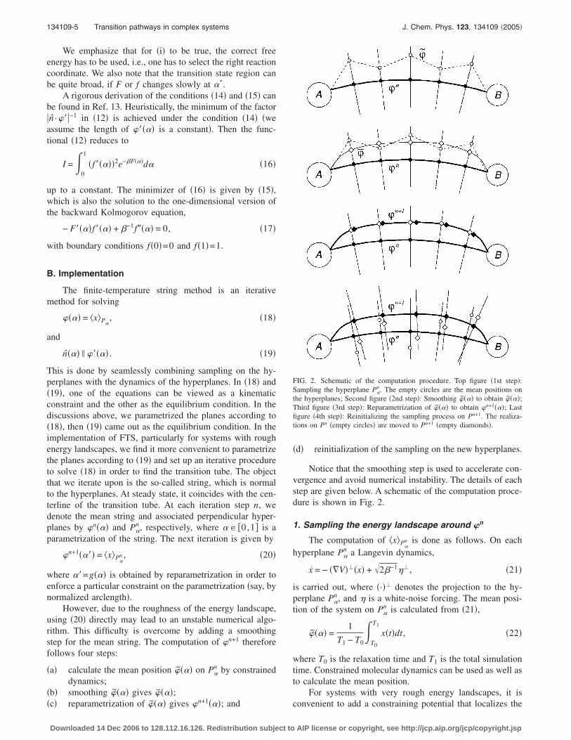
Notice that the smoothing step is used to accelerate con-vergence and avoid numerical instability. The details of eachstep are given below. A schematic of the computation proce-dure is shown in Fig. 2.

1. Sampling the energy landscape around �n

The computation of �x Pn is done as follows. On each

hyperplane Pn a Langevin dynamics,

x = − ��V��x� + �2�−1��, �21�

is carried out, where �·�� denotes the projection to the hy-perplane P

n , and � is a white-noise forcing. The mean posi-tion of the system on P

n is calculated from �21�,

�� =1

T1 − T0�

T0

T1

x�t�dt , �22�

where T0 is the relaxation time and T1 is the total simulationtime. Constrained molecular dynamics can be used as well asto calculate the mean position.

For systems with very rough energy landscapes, it is

FIG. 2. Schematic of the computation procedure. Top figure �1st step�:Sampling the hyperplane P

n . The empty circles are the mean positions onthe hyperplanes; Second figure �2nd step�: Smoothing �� to obtain ��;Third figure �3rd step�: Reparametrization of �� to obtain n+1��; Lastfigure �4th step�: Reinitializing the sampling process on Pn+1. The realiza-tions on Pn �empty circles� are moved to Pn+1 �empty diamonds�.

convenient to add a constraining potential that localizes the



sampling in �21� to region close to the current mean string.This is again used to avoid numerical instability, but has noeffect on the final result. The following potential is used inour calculation:

Vc�x� = �0, r � c

�r − d�−12 − 2��c − d��r − d��−6, c � r � d

, r � d .��23�

Here r= x−n , n is the current mean string and c and d arethe two parameters. Under this constraining force, samplingin �21� is confined in a tube with radius d around the currentmean string. Moreover, the system experiences no constrain-ing force in a even smaller tube with radius c. The constrain-ing force is gradually switched off as the computation con-verges. This is done by gradually increasing the confiningparameter c.

2. Smoothing the mean string

The calculated mean string �� may not be verysmooth and this may make the tangent vector so inaccuratethat it introduces numerical instabilities. Therefore at eachiteration, we smooth out �� by solving the following op-timization problem:

min��

�0

1

�C1�� + C2�� − ��M�d . �24�

Here �� is the curvature of �� and �x�M = �x ,Mx�1/2 isthe L2 norm of x weighted by M = �C��+ I�−1, where C�� isthe covariance matrix of x generated by constrained dynam-ics on each hyperplane. The parameters C1 , C2� �0,1� de-termine the relative weights of the two terms. As two ex-treme cases, the solution of �24� is a line segment when C1

=1 and C2=0 and the solution ��= �� when C1=0 andC2=1.

The minimization problem �24� can be solved by thesteepest-descent method, or more advanced techniques, e.g.,the quasi-Newton �Broyden-Fletcher-Goldfarb-Shanno�BFGS�� method.

3. Reparameterization

At the third step of each iteration, the mean string ��is reparametrized, for example, by normalized arclength, togive n+1��. The reparametrization is done by polynomialinterpolation.1

4. Reinitialization

A new collection of hyperplanes Pn+1 which are orthogo-

nal to n+1�� are obtained after the reparametrization step.To start the sampling process on the new planes, we need togenerate the initial configurations for the Langevin dynamics�21�. A naive way to generate the initial configurations is toproject the realizations on P

n from the previous samplingprocess onto the new planes P

n+1. But unfortunately this pro-cedure usually result in abrupt changes in the molecularstructure and thus very large potential force. In the case that
the artificial constraining potential �23� is used, the direct

projection becomes even worse since it is possible that theprojected realizations are out of the tube defined by the con-straining potential and thus have infinite force.

In our implementation, this difficulty is overcome by

inserting a few intermediate hyperplanes, denoted by Pj , j=0,1 ,… ,J�, in between P

n and Pn+1, and each time we

project the realization from Pj to Pj+1, followed by a few

steps of relaxation on Pj+1. This is analogous to choosingsmall time steps for numerical stability when solving ordi-nary differential equations �ODEs� or partial differential

equations �PDEs�. Here P0= Pn , PJ= P

n+1, and Pj , j=1,… ,J−1� are obtained by linear interpolation between P

n

and Pn+1, i.e., the unit normals are given by

nj = c��1 −j

J�n0 +

j

JnJ�, j = 1,2,…J − 1, �25�

where n0 and nJ are the unit normals to Pn and P

n+1, respec-tively, and c is the normalization factor. The interpolated

plane Pj goes through � j, where � j is given by

� j = �1 −j

J��0 +

j

J�J, j = 1,2,…J − 1, �26�

where �0=n and �J=

n+1. On each interpolated hyperplane

Pj, the constraining force �23� is centered at � j.For each , we move the realization x on P

n to Pn+1 in J

steps. At the jth step, j=1,2 ,… ,J, we first project x from

Pj−1 to Pj,

x ª x − ��x − � j� · nj�nj . �27�

Then we relax the projected configuration on Pj for a shorttime T2 �a few time steps�,

x�t� = − ��V��,j�x� + �2�−1��,j, 0 � t � T2, �28�

where ��V��,j =�V− ��V , nj�nj and V�x� includes the poten-tial of the system and the constraining potential. Similar pro-jection is done for �.

In the following application to the alanine dipeptide, theparameter T2 is taken to be a few time steps for �28�, andJ=10.

Sampling on the new hyperplanes Pn+1 begins after weobtain the new set of realizations, and the above four-stepprocedure repeats.

When the iteration converges with satisfactory accuracy,the mean string gives the centerline of the tube, the varianceof x�� on the hyperplanes give the width of the transitiontube, and the function f�� in �15� gives the committor valueof each plane. To obtain f��, the free energy �13� must becomputed, which can be done by calculating the mean forceby sampling via �21� on the final planes, and thermodynamicintegration.

IV. APPLICATION TO THE ALANINE DIPEPTIDE

The ball and stick model of the alanine dipeptide isshown in Fig. 3. Despite its simple chemical structure, itexhibits some of the important features common to biomol-
ecules, with the backbone degree of freedoms �dihedral


angles � and ��, three methyl groups �CH3�, as well as thepolar groups �N–H and CvO� which form hydrogen bondswith water in aqueous solution. The isomerization of alaninedipeptide has been the subject of several theoretical andcomputational studies and therefore serves as an excellenttest for FTS.

Apostolakis et al. calculated the transition pathways andbarriers for the isomerization of alanine dipeptide.17 In theirwork, a two-dimensional potential of mean force on the�-� plane was first calculated by the adaptive umbrella sam-pling scheme. The conjugate peak refinement algorithm andtargeted molecular-dynamics technique were applied on theobtained two-dimensional potential to obtain the transitionpathways. As a result, the mechanism of the transition ispreassumed to depend only on the two torsion angles � and�. Bolhuis et al. applied TPS to study the isomerization ofalanine dipeptide in vacuum and in solution.18 Their calcula-tion used the all-atom representation for the molecule andexplicit solvent model. An ensemble of transition pathwayswas collected, from which the transition state ensemble wasfound by determining the committor for each configurationvisited by the trajectories. Their analysis shows that moredegrees of freedom than the two torsion angles are necessaryto describe the reaction coordinates. Recently, Ma and Din-ner introduced a statistical method for identifying reactioncoordinates from a database of candidate physical variables,and applied their method to study the isomerization of ala-nine dipeptide.15 In the following, we apply FTS to study thetransition of the alanine dipeptide both in vacuum and inexplicit solvent.

A. Alanine dipeptide in vacuum

We use the full atomic representation of the alaninedipeptide molecule with the CHARMM22 force field.19 Wehave not used the CMAP correction to the dihedral anglepotentials20 since it is unclear how the CMAP correction in-fluences the dynamics of proteins. Figure 4 shows the adia-batic energy landscape of the molecule as a function of thetwo backbone dihedral angles � and �. There are two stableconformers C7eq and Cax. The state C7eq is further split intotwo sub-states �denoted by C7eq and C7eq� in Fig. 4� separated

FIG. 3. Schematic representation of the alanine dipeptide�CH3–CONH–CHCH3–CONH–CH3�. The backbone dihedral angles are la-beled by �: C–N–C–C and �: N–C–C–N. The picture is taken from Ref. 18.

by a small barrier.


Normally, one needs to identify the initial and final statesbefore FTS can be used. This case is different since there issome periodicity in the system. The initial string �and therealizations on each hyperplane� is obtained by rotating thetwo backbone dihedral angles of the dipeptide along the di-agonal line from �−180°, 180°� to �180°, −180°�, with allother internal degrees of freedom kept fixed. Only nonhydro-gen atoms are represented on the string. The string is dis-cretized using 40 points and correspondingly 40 hyperplanesare evolved in the computation. At each iteration, time aver-aging is performed for 0.5 ps following the dynamics de-scribed in �21� with T=272 K. A hard-core constraining po-tential is added to restrict the sampling to a tube with widthof 0.2 Å �c=0.2 and d=1 in �23�� around the string. Thisconstraint is gradually removed as the string converges to thesteady state. The parameters used in smoothing the string areC1=C2=1.

To fix the overall rotation and translation of the mol-ecule, we constrained one carbon atom at the origin, oneneighboring carbon atom at the positive x axis, and one ni-trogen atom in the xy plane by harmonic springs. The com-putation converges after about 60–70 iterations. It takesabout several-hour CPU time on a single processor personalcomputer �PC�.

The converged string and the tube are shown in Fig. 5.This tube is represented by projecting onto the �-� plane theensemble of the realizations on each hyperplane correspond-ing to the converged string. As we discussed earlier, this tubeshould coincide with the tube obtained from the most prob-able transition paths between the stable conformers Cax andC7eq. The free energy F along the string is shown in Fig. 6�upper panel�. The free energy has three local maxima S1, S2,and S3, corresponding to the two transition pathways fromCax to C7eq: �a� Cax–S1–C7eq� –S2–C7eq and �b� Cax–S3–C7eq.The transition at S1 and S3 is quite sharp. The energy differ-ence of Cax relative to C7eq is about E=2.5 kcal/mol. Theenergy barrier is about �E=7.0 kcal/mol at S1, and about

FIG. 4. �Color� Adiabatic energy landscape of the alanine dipeptide. Theenergy landscape is obtained by minimizing the potential energy of themolecule with �� ,�� fixed. The contours are drawn at multiples of1 kcal/mol above the C7eq minimum. There are two stable conformers C7eq

and Cax.

�E=7.5 kcal/mol at S3. Path �a� goes through an intermedi-



ate metastable state C7eq� around �−150°, 170°�. But the en-ergy barrier from C7eq� to C7eq is comparable to kBT and it haslittle effect on the transition from Cax to C7eq.

Shown in the lower panel of Fig. 6 is the committorfunction f�� to the state Cax for the pathway C7eq–S3–Cax

calculated using the formula �15�. The transition state regionis identified as the hyperplane labeled by � that satisfiesf��= 1

2 . This plane is close to the one with maximum freeenergy between C7eq and Cax

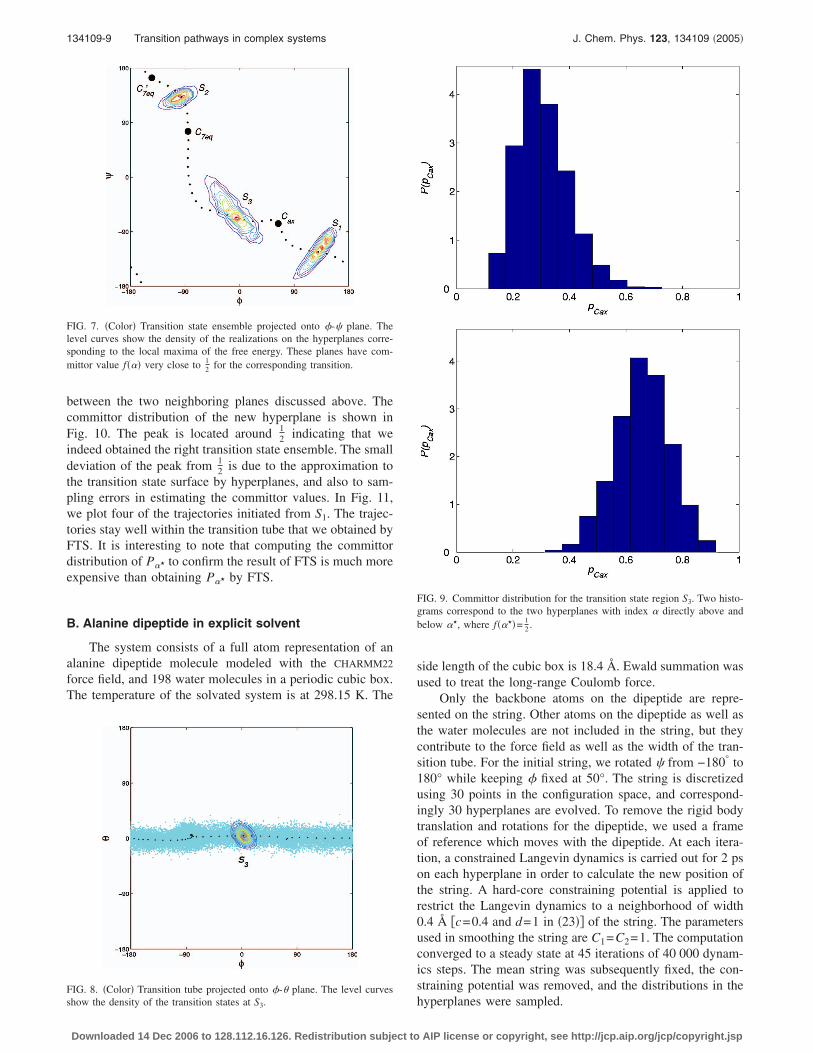
Figure 7 shows the projection of the level curves of theequilibrium probability density on the hyperplanes corre-sponding to the local maxima of the free energy. We see thatat S1 and S2, the projected transition states are localized onlines which are roughly perpendicular to the projected meanpath �dotted line�, which suggests that the two backbone di-hedral angles may parametrize reasonably well the reactioncoordinate q�x� for this transition. However, the projectedtransition states at S3 spread out in �-� plane and are nolonger concentrated on the line perpendicular to the pro-jected mean path. This indicates that, in addition to � and �,there are other degree of freedoms that are important for thistransition. In Ref. 18, the calculation by TPS shows that anadditional torsion angle � plays an important role in thistransition, and the angles � and � provides a good set ofcoarse variables to parametrize the reaction coordinate q�x�.However, our calculation shows that the angle � is approxi-mately constant along the transition tube, and the projectedtransition states on �-� plane is still quite broad and far frombeing concentrated on the line perpendicular to the projectedmean string �see Fig. 8�. Therefore, we conclude that � and� are not sufficient to parametrize the reaction coordinateq�x�. This discrepancy may be due to the different forcefields used in the two calculations: We used the CHARMM22

FIG. 5. The transition tube between C7eq and Cax. Two pathways exist: �a�Cax–S1–C7eq� –S2–C7eq and �b� Cax–S3–C7eq. The dotted line is the path of�� ,�� along the mean string. The converged hyperplanes across the pointsdenoted by diamonds are approximations to the transition state surfaces.

force field, and the authors in Ref. 14 used AMBER.


To see that we indeed obtained the right transition tubeand transition state ensemble, we computed the committordistribution of the plane P� for which f��= 1

2 by initiatingtrajectories from this plane �this plane corresponds to thetransition state region S3�. Recall that in our calculation thestring is discretized to a collection of points parametrized byi�. In general � in Fig. 6 is not in this discrete set. Tocompensate for this, we compute the committor distributionfor the two neighboring hyperplanes, one on each side of �.We randomly picked 2490 points based on the equilibriumdistribution on each of the two planes. Starting from each ofthese points, 5000 trajectories were launched, from whichthe committor distribution PCax

or the probability that thetrajectory goes to Cax is calculated. Figure 9 shows the dis-tribution of PCax

. The distribution is peaked at PCax=0.3 and

PCax=0.7, respectively. This confirms our prediction that the

transition state region must be in between these two hyper-planes.

FIG. 6. Top figure: Free energy of the alanine dipeptide along the transitiontube shown in Fig. 5; Lower figure: Committor f�� along the pathC7eq–S3–Cax. The transition state ensemble for the transition C7eq–S3–Cax ison the hyperplane labeled by � determined by f��= 1

2 . Note that thisplane is also very close to the one with maximum free energy between C7eq

and Cax.

We next refined the string and added one more plane



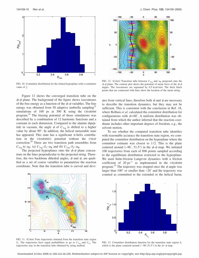
between the two neighboring planes discussed above. Thecommittor distribution of the new hyperplane is shown inFig. 10. The peak is located around 1

2 indicating that weindeed obtained the right transition state ensemble. The smalldeviation of the peak from 1

2 is due to the approximation tothe transition state surface by hyperplanes, and also to sam-pling errors in estimating the committor values. In Fig. 11,we plot four of the trajectories initiated from S1. The trajec-tories stay well within the transition tube that we obtained byFTS. It is interesting to note that computing the committordistribution of P� to confirm the result of FTS is much moreexpensive than obtaining P� by FTS.

B. Alanine dipeptide in explicit solvent

The system consists of a full atom representation of analanine dipeptide molecule modeled with the CHARMM22

force field, and 198 water molecules in a periodic cubic box.The temperature of the solvated system is at 298.15 K. The

FIG. 7. �Color� Transition state ensemble projected onto �-� plane. Thelevel curves show the density of the realizations on the hyperplanes corre-sponding to the local maxima of the free energy. These planes have com-mittor value f�� very close to 1

2 for the corresponding transition.

FIG. 8. �Color� Transition tube projected onto �-� plane. The level curves
show the density of the transition states at S3.

side length of the cubic box is 18.4 Å. Ewald summation wasused to treat the long-range Coulomb force.

Only the backbone atoms on the dipeptide are repre-sented on the string. Other atoms on the dipeptide as well asthe water molecules are not included in the string, but theycontribute to the force field as well as the width of the tran-sition tube. For the initial string, we rotated � from −180° to180° while keeping � fixed at 50°. The string is discretizedusing 30 points in the configuration space, and correspond-ingly 30 hyperplanes are evolved. To remove the rigid bodytranslation and rotations for the dipeptide, we used a frameof reference which moves with the dipeptide. At each itera-tion, a constrained Langevin dynamics is carried out for 2 pson each hyperplane in order to calculate the new position ofthe string. A hard-core constraining potential is applied torestrict the Langevin dynamics to a neighborhood of width0.4 Å �c=0.4 and d=1 in �23�� of the string. The parametersused in smoothing the string are C1=C2=1. The computationconverged to a steady state at 45 iterations of 40 000 dynam-ics steps. The mean string was subsequently fixed, the con-straining potential was removed, and the distributions in the

FIG. 9. Committor distribution for the transition state region S3. Two histo-grams correspond to the two hyperplanes with index directly above andbelow �, where f��= 1

2 .

hyperplanes were sampled.



Figure 12 shows the converged transition tube on the�-� plane. The background of the figure shows isocontoursof the free energy as a function of the �-� variables. The freeenergy was obtained from 50 adaptive umbrella sampling21

simulations of 100 ps at 300 K using the CHARMM

program.22 The biasing potential of those simulations wasdescribed by a combination of 12 harmonic functions and aconstant in each dimension. Compared to the alanine dipep-tide in vacuum, the angle � of C7eq is shifted to a highervalue by about 90°. In addition, the helical metastable statehas appeared. This state has a significant �-helix contribu-tion in the CHARMM22 potential without the CMAP

correction.20 There are two transition path ensembles fromC7eq to R: �a� C7eq–S1–R and �b� C7eq–S2–R.

The projected hyperplanes onto the �-� plane concen-trate on the lines perpendicular to the projected string. There-fore, the two backbone dihedral angles, � and �, are quali-fied as a set of coarse variables to parametrize the reactioncoordinate. Note that the transition tube is curved and devi-

FIG. 10. Committor distribution for the refined hyperplane with a committorvalue of 1

2 .

FIG. 11. �Color� Four trajectories initiated from the transition state regionS1. The trajectories have equal probabilities to go to C7eq and Cax. The
trajectories stay in the transition tube obtained by string method.

ates from vertical lines, therefore both � and � are necessaryto describe the transition dynamics, but they may not besufficient. This is consistent with the conclusion in Ref. 18,where Bolhuis et al. calculated the committor distribution forconfigurations with �=60°. A uniform distribution was ob-tained from which the author inferred that the reaction coor-dinate includes other important degrees of freedom, e.g., thesolvent motion.

To see whether the computed transition tube identifieswith reasonable accuracy the transition state region, we com-puted the committor distribution on the hyperplane where thecommittor estimate was closest to 1 /2. This is the planecentered around �−96°, 51.5°� in the �-� map. We initiated100 trajectories from each of 896 points sampled accordingto the equilibrium distribution restricted to the hyperplane.We used finite-friction Langevin dynamics with a frictioncoefficient of 20 ps−1 as implemented in the CHARMM

program.22 The trajectory was stopped once the � angle waslarger than 100° or smaller than −20° and the trajectory wascounted as committed to the extended or the helical basin,

FIG. 12. �Color� Transition tube between C7eq and R projected onto the�-� plane. The contour plot shows the potential of mean force of the �-�angles. The isocontours are separated by 0.5 kcal/mol. The thick blackpoints that are connected with lines show the location of the mean string.

FIG. 13. Committor distribution function for the transition state region S1

which is the plane centered around ��96°,51.5°� in the �−� map.



respectively. Due to the very long commitment times re-quired by these trajectories, we limited ourselves to a smallerensemble than in the vacuum study. The calculated commit-tor distribution is shown in Fig. 13. The distribution ispeaked around 1

2 , but it is less peaked than the one obtainedin vacuum. The average value of the committor distributionis 0.50 and the standard deviation is 0.21. One component ofthe distribution width is due to the limited sampling of theensemble by only 100 trajectories per initial condition. Thelimited sampling by only 100 trajectories per initial condi-tion contributes a standard deviation of 0.05 to the results ofsampling a sharp 0.5 committor isosurface. The remainingpart of the error is due to the approximation of the hypersur-faces by hyperplanes and due to the assumption that the iso-committors can be described on the peptide backbone de-grees of freedom.

Figure 14 shows the four typical reactive trajectories.These trajectories have equal probability to fall into C7eq orR, and they follow the transition tube quite well. Comparedto the behavior in vacuum, the dynamics of the solvatedsystem is quite diffusive due to the collisions with watermolecules and the lack of a high energetic barrier in thetransition region.

V. CONCLUSIONS

In this paper FTS was successfully applied to study thetransition events of the alanine dipeptide in vacuum and inexplicit solvent. The results of FTS were justified by launch-ing trajectories from the transition state region and the cal-culation of the committor distributions to confirm that FTSallows one indeed to find isocommittor surfaces, in particu-lar, the one with committor value of 1

2 corresponding to thetransition state region.

It is illuminating to make a comparison between the phi-losophies behind TPS and FTS. TPS and FTS are after thesame objects, namely, the ensemble of transition paths andtransition states. Their key difference is in the way that thetransition paths are parametrized. TPS considers transition

FIG. 14. �Color� Four typical trajectories initiated from the transition stateregion S1. The trajectories have equal probability to go to C7eq and R, andthey follow the transition tube.

paths in the space of physical trajectories, parametrized by


the real time. FTS considers transition paths in configurationspace, parametrized, for example, by the arclength of thecenterline of the transition tube. This different parametriza-tion gives FTS considerable advantage. First, the ensembleof transition paths can be characterized by equilibrium den-sities, if we consider where they hit the isocommittor sur-faces. Second, this allows us to give a direct link between thetransition path ensemble and the transition state ensemble. Inaddition, it also allows us to develop sampling procedures bywhich a collection of paths are harvested at the same time,instead of one by one as in TPS. In other words FTS allowsone to bypass completely the calculation of reactive trajec-tories parametrized by time and directly obtain the isocom-mittor surfaces and the transition tubes which are more rel-evant to describe the mechanism of the transition.

To conclude, FTS is a powerful tool for determining theeffective transition pathways in complex systems with mul-tiscale energy landscapes. It does not require specifying areaction coordinate beforehand. It allows us to determine thehyperplanes which are approximations to the isocommittorsurfaces in configuration space by evolving a smooth curve.The smooth curve converges to the center of a tube by whichtransitions occur with high probability.

Note added in proof: It was brought to our attention thatEq. �6� was derived in G. Hummer,23 in the simpler contextof a one-dimensional diffusion process.

ACKNOWLEDGMENTS

The authors thank M. Karplus for helpful discussions.Two of the authors �W. E� and �E. V.-E.� were partially sup-ported by ONR Grant Nos. N00014-01-1-0674 and N00014-04-1-0565, and NSF Grant Nos. DMS01-01439, DMS02-09959, and DMS02-39625. Another author �P.M.�acknowledges support by the Marie Curie European Fellow-ship Grant No. MEIF-CT-2003-501953. The explicit watercalculations were performed in the Crimson Grid cluster atHarvard, the SDSC teragrid and the CIMS computer center.

APPENDIX: DERIVATION OF „12…

We derive the formula �12� from �10�,

I = ��

�q2e−�Vdx

= ��

�q2e−�V�0

1

��q�x� − z�dzdx

= �0

1

dz��

�q2e−�V��q�x� − z�dx

= �0

1

f��d��

�qe−�V��n · �x − ��dx

= �0

1

f��q��d��

e−�V��n · �x − ��dx

= �1

f��2�n · ��−1e−�F��d . �A1�
0


Here we denote � \ �A�B� by ��. To go from the third to thefourth line, we made the assumption that the isocommittorsurface is locally planar with normal n, and defined f��=q��. To go from the fourth to the fifth line, we used thefollowing assumption:

��n� · �x − ��2 P� �n · ��2, �A2�

where the average is with respect to the equilibrium distri-bution restricted to P. In the last step, we defined the freeenergy F�� as in �13� and used f��=�q�� ·�= �q��n ·��.

1 W. E, W. Ren, and E. Vanden-Eijnden, Phys. Rev. B 66, 052301 �2002�.2 W. E, W. Ren, and E. Vanden-Eijnden, J. Phys. Chem. B 109, 6688�2005�.

3 H. Jónsson, G. Mills, and K. W. Jacobsen, in Classical and QuantumDynamics in Condensed Phase Simulations, edited by B. J. Berne, G.Ciccoti, and D. F. Coker �World Scientific, Singapore, 1998�.

4 W. E, W. Ren, and E. Vanden-Eijnden �unpublished�.5 S. Fischer and M. Karplus, Chem. Phys. Lett. 194, 252 �1992�.6 I. V. Ionova and E. A. Carter, J. Chem. Phys. 98, 6377 �1993�.7 G. Henkelman and H. Jónsson, J. Chem. Phys. 111, 7010 �1999�.8 L. R. Pratt, J. Chem. Phys. 85, 5045 �1986�.


9 E. A. Carter, G. Ciccotti, J. T. Hynes, and R. Kapral, Chem. Phys. Lett.156, 472 �1989�.

10 P. G. Bolhuis, D. Chandler, C. Dellago, and P. Geissler, Annu. Rev. Phys.Chem. 59, 291 �2002�.

11 C. Dellago, P. G. Bolhuis, and P. L. Geissler, Adv. Chem. Phys. 123�2002�.

12 W. E, W. Ren, and E. Vanden-Eijnden, Chem. Phys. Lett. 413, 242�2005�.

13 W. E and E. Vanden-Eijnden, in Multiscale Modeling and Simulation,edited by S. Attinger and P. Koumoutsakos LNCSE Vol. 39, �Springer,Berlin, 2004�.

14 R. Olender and R. Elber, J. Chem. Phys. 105, 9299 �1996�.15 A. Ma and A. Dinner, J. Phys. Chem. B 109, 6769 �2005�.16 C. W. Gardiner, Handbook of Stochastic Methods for Physics, Chemistry,

and the Natural Sciences �Springer, New York, 1997�.17 J. Apostolakis, P. Ferrara, and A. Caflisch, J. Chem. Phys. 10, 2099

�1999�.18 P. G. Bolhuis, C. Dellago, and D. Chandler, Proc. Natl. Acad. Sci. U.S.A.

97, 5877 �2000�.19 A. D. MacKerell, D. Bashford, M. Bellott et al., J. Phys. Chem. B 102,

3586 �1998�.20 M. Feig, A. D. MacKerell, and C. L. Brooks, J. Phys. Chem. B 107, 2831

�2003�.21 C. Bartels and M. Karplus, J. Comput. Chem. 18, 1450 �1997�.22 B. R. Brooks, R. E. Bruccoleri, B. D. Olafson, D. J. States, S. Swami-

nathan, and M. Karplus, J. Comput. Chem. 4, 187 �1983�.23 G. Hummer, J. Chem. Phys. 120, 516 �2004�.


Documents

Transition pathways in complex systems: Application of the