Embed Size (px)
Citation preview
Revista Colombiana de EstadísticaJanuary 2017, Volume 40, Issue 1, pp. 1 to 27
DOI: http://dx.doi.org/10.15446/rce.v40n1.50085
Transmuted Singh-Maddala Distribution: A newFlexible and Upside-Down Bathtub Shaped
Hazard Function Distribution
Distribución Singh-Maddala transmutada: una nueva distribución,flexible y con forma de bañera invertida para la función de riesgo
Mirza Naveed Shahzad1,a, Faton Merovci2,b, Zahid Asghar3,c
1Department of Statistics, University of Gujrat, Gujrat, Pakistan2University of Prishtina ”Hasan Prishtina“, Pristina, Republic of Kosovo3Department of Statistics, Quaid-i-Azam University, Islamabad, Pakistan
Abstract
The Singh-Maddala distribution is very popular to analyze the data on in-come, expenditure, actuarial, environmental, and reliability related studies.To enhance its scope and application, we propose four parameters trans-muted Singh-Maddala distribution, in this study. The proposed distributionis relatively more flexible than the parent distribution to model a variety ofdata sets. Its basic statistical properties, reliability function, and behaviorsof the hazard function are derived. The hazard function showed the decreas-ing and an upside-down bathtub shape that is required in various survivalanalysis. The order statistics and generalized TL-moments with their specialcases such as L-, TL-, LL-, and LH-moments are also explored. Furthermore,the maximum likelihood estimation is used to estimate the unknown param-eters of the transmuted Singh-Maddala distribution. The real data sets areconsidered to illustrate the utility and potential of the proposed model. Theresults indicate that the transmuted Singh-Maddala distribution models thedatasets better than its parent distribution.
Key words: Moments, Parameter Estimation, Transmuted Singh-MaddalaDistribution, TL-Moments, Upsidedown Bathtub Shaped Hazard Rate.
aPhD. E-mail: [email protected]. E-mail: [email protected]. E-mail: [email protected]
1
2 Mirza Naveed Shahzad, Faton Merovci & Zahid Asghar
ResumenLa distribución Singh-Maddala es muy popular para analizar datos de
ingresos, gastos, actuariales, ambientales y de confiabilidad.Para mejorar su alcance y aplicación se propone su extensión a la dis-
tribución de cuatro parámetros Singh-Maddala transmutada. Esta es másflexible en la modelación de diversos conjuntos de datos. Sus propiedadesbásicas, las funciones de confiabilidad y riesgos son estudiadas. La funciónde riesgo es decrecientes o tiene forma de bañera invertida. Como se requiereen varios estudios de sobrevivencia se exploran sus estadísticas de orden y losmomentos TL, con sus casos especiales L, TL, LL y LH. Se emplea máximaverosimilitud para la estimación de los cuatro parámetros. Datos reales sonusados para ilustrar la utilidad y potencialidad del modelo propuesto. Losresultados indican que la distribución propuesta ajusta mejor que la original.
Palabras clave: distribución Singh-Maddala transmuetada, función de riesgoinvertida, momentos, momentos TL, estimación de parámetros.
1. Introduction
The quality of the statistical analysis heavily depends on the assumed prob-ability distribution. Therefore, the most attractive research direction for math-ematicians and statisticians is to develop a class of suitable distributions, alongwith their relevant statistical properties and methodologies. The goal is to designthe standard probability distributions which serve as true models for real worldsituations. However, there are still many important symmetric and asymmetricspaces present where the existing distributions do not follow the real data pattern.Keeping this in mind, we selected Shaw & Buckley (2009) proposed quadratic ranktransmutation map that is applicable for both symmetric and asymmetric distri-butions. This map is a special case of the general rank transmutation map and itis defined by Shaw & Buckley (2009) without loss of generality. It is given as
TR12(u) = F{G−1(u)},
TR21(u) = G{F−1(u)},
where G and F are the two cumulative distribution functions on a common samplespace, and G−1 and F−1 are their quantile functions, respectively.
The two functions TR12(u) and TR21(u) map the unit interval I = [0, 1] intoitself, and under suitable assumptions they satisfy Tij(0) = 0 and Tji(1) = 1. Thisrank transmutation should be continuously differentiable otherwise discontinuitymay occur in the transmuted density. Now the quadratic rank transmutation isdefined for −1 ≤ λ ≤ 1 as,
TR(u) = u+ λu(1− u),
which results in the cumulative distribution function of the transmuted probabilitydistribution as follows
F (x) = G(x)[(1 + λ)− λG(x)
](1)
Revista Colombiana de Estadística 40 (2017) 1–27
Transmuted Singh Distribution 3
that yields the probability density function on differentiation and is given as
f(x) = g(x)[(1 + λ)− 2λG(x)
]. (2)
Where g(x) and G(x) are the probability density and cumulative distributionfunctions of the parent distribution, respectively. The parameter λ lies between[−1, 1] and the extreme values of the λ produce two extreme cases. These casesgenerate the distribution of the maximum and minimum for λ = −1 and λ = +1,F (x) = G(x)2, and F (x) = G(x)[2−G(x)], respectively. It is also observed, whenλ = 0 that the transmuted distribution exactly approaches the parent distribution.
This recent quadratic rank transmutation map is used in many studies to ob-tain a flexible and versatile model. Sharma, Singh & Singh (2014) proposed thetransmuted inverse Rayleigh distribution and used this density function in survivalanalysis because its hazard function has the upside-down bathtub shape. Khan &King (2014) proposed a generalized transmuted inverse Weibull distribution andfound it to found better than the parent distribution in real data application.Similar interpretation are also observed by Shahzad & Asghar (2016), Ahmad,Ahmad & Ahmed (2014), Khan, King & Hudson (2014), Aryal (2013), Merovci(2013), Elbatal (2013) and Aryal & Tsokos (2011).
The rest of the paper is organized as follows: In Section 2, we have derived andsketched the pdf and cdf of transmuted Singh-Maddala distribution. In Section3, rth moment, moment generating function, quantile function, and random num-ber generating process for transmuted Singh Maddala distribution are explored.Survival analysis of the distribution such as the reliability function and hazardrate function are obtained and presented graphically in Section 4. In Section 5,order statistics and the densities of lowest, highest, and joint order statistics arespecified. Section 6 is about the TL-moments and its special cases. Methodologyfor parameter estimation is discussed in Section 7. The real data set applicationof the transmuted Singh-Maddala distribution is given in Section 8, and finallystudy is concluded in Section 9.
2. Transmuted Singh-Maddala Distribution
The Singh-Maddala is a well-known distribution and is attributed to Singh &Maddala (1976). It was initially used for modeling income data analysis, but dueto its better performance it is now popular in a range of fields including actuar-ial science, economics, extreme value, and reliability studies. Zimmer, Keats &Wang (1998) studied this model and concluded that the model perform better forcertain failure time data analysis. Shao, Wang & Zhang (2013) applied the ex-tended Singh-Maddala (SM) distribution to flood frequency analysis. Brzezinski(2014) modeled the empirical impact factor distribution and observed that theSM distribution performance is much better than those of the models which werepreviously applied to this type of data. Sakulski, Jordaan, Tin & Greyling (2014)quantified several statistical distributions for the analysis of rainfall data such asExtreme Value, Frechet, Log-normal, Log-logistic, Rice, SM, and Rayleigh proba-bility distributions for summer, autumn, winter and spring seasons. Finally, they
Revista Colombiana de Estadística 40 (2017) 1–27
4 Mirza Naveed Shahzad, Faton Merovci & Zahid Asghar
stated that for all seasons SM distribution fits acutely well. There is wide mono-graphic and periodical literature available on it, for example see, Kleiber & Kotz(2003). To enhance its applicability in various other fields, we introduced thetransmuted Singh-Maddala distribution in this section. The transmuted Singh-Maddala (TSM) is more versatile and flexible than the SM distribution.
The TSM distribution is proposed using the quadratic rank transmutation map,taking the SM distribution as a parent distribution. Let X be a random sampleof size n and come from the SM distribution with the pdf that has the followingform:
g(x;α, β, δ) =αδxα−1
βα[1 + (x/β)α
]δ+1, 0 ≤ x ≤ ∞. (3)
Its cdf is asG(x;α, β, δ) = 1− 1[
1 + (x/β)α]δ , (4)
where α and δ are the shape parameters (α, δ > 0), β is the scale parameter(β > 0).The cdf and pdf of the TSM distribution is derived using (3) and (4) in the trans-mutation mapping given in (1) and (2). The cdf and pdf of the TSM distributionare obtained in the following form
F (x;α, β, δ, λ) =[1−
[1 + (x/β)α
]−δ][1 + λ
[1 + (x/β)α
]−δ] (5)
and
f(x;α, β, δ, λ) =αδxα−1
[2λ+ (1− λ)
[1 + (x/β)α
]δ]βα[1 + (x/β)α
]2δ+1, (6)
respectively.In TSM distribution, the parameter λ is the transmutation parameter that
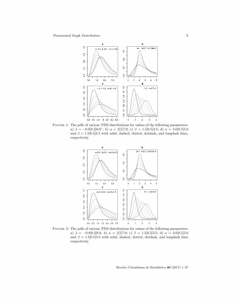
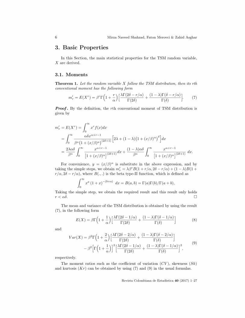
lies between [−1, 1]. TSM distribution becomes very appealing and applicabledue to its flexibility as it provides a more accurate fitting with the complex data.The shapes of the pdf and cdf of the TSM distribution for various combinationsof all the four parameters are sketched in Figure 1 and Figure 2, respectively.These figures indicate that the TSM density demonstrates more flexibility thanthe parent SM distribution.
Note:∗ Here the representation α[i]β, shows the different values of the param-eter, those starts from α and approachs β with the increment of i.
Revista Colombiana de Estadística 40 (2017) 1–27
Transmuted Singh Distribution 5
Figure 1: The pdfs of various TSM distributions for values of the following parameters:a) λ = −0.8[0.2]0.6∗; b) α = 2[1]7.0; c) β = 1.5[0.5]3.5; d) α = 3.0[0.5]5.0and β = 1.5[0.5]3.5 with solid, dashed, dotted, dotdash, and longdash lines,respectively.
0.0 1.0 2.0 3.0
0.0
0.2
0.4
0.6
0.8
a
α=2.5, β=2.0 and δ=2.0
0 1 2 3 4 5
0.0
0.2
0.4
0.6
b
β=1 λ=0.3 and δ=0.4
0.0 0.5 1.0 1.5 2.0 2.5 3.0
0.0
0.2
0.4
0.6
0.8
1.0
c
α=2 λ=0.8 and δ=1.8
0 1 2 3 4
0.0
0.2
0.4
0.6
0.8
1.0
1.2
d
λ=1 and δ=2
Figure 2: The pdfs of various TSM distributions for values of the following parameters:a) λ = −0.8[0.2]0.6; b) α = 2[1]7.0; c) β = 1.5[0.5]3.5; d) α = 3.0[0.5]5.0and β = 1.5[0.5]3.5 with solid, dashed, dotted, dotdash, and longdash linesrespectively.
Revista Colombiana de Estadística 40 (2017) 1–27
6 Mirza Naveed Shahzad, Faton Merovci & Zahid Asghar
3. Basic Properties
In this Section, the main statistical properties for the TSM random variable,X are derived.
3.1. Moments
Theorem 1. Let the random variable X follow the TSM distribution, then its rthconventional moment has the following form
m′r = E(Xr) = βrΓ(
1 +r
α
)[λΓ(2δ − r/α)
Γ(2δ)+
(1− λ)Γ(δ − r/α)
Γ(δ)
]. (7)
Proof . By the definition, the rth conventional moment of TSM distribution isgiven by
m′r = E(Xr) =
∫ ∞0
xrf(x)dx
=
∫ ∞0
αδxα+r−1
βα(1 + (x/β)α
)(2δ+1)
[2λ+ (1− λ)
(1 + (x/β)α
)δ]dx
=2λαδ
βα
∫ ∞0
xα+r−1[1 + (x/β)α
](2δ+1)dx+
(1− λ)αδ
βα
∫ ∞0
xα+r−1[1 + (x/β)α
](2δ+1)dx.
For convenience, y = (x/β)α is substitute in the above expression, and bytaking the simple steps, we obtain m′r = λβrB(1 + r/α, 2δ − r/α) + (1− λ)B(1 +r/α, 2δ − r/α), where B(., .) is the beta type-II function, which is defined as∫ ∞
0
xa (1 + x)−(b+a)
dx = B(a, b) = Γ(a)Γ(b)/Γ(a+ b),
Taking the simple step, we obtain the required result and this result only holdsr < αδ.
The mean and variance of the TSM distribution is obtained by using the result(7), in the following form
E(X) = βΓ(
1 +1
α
)[λΓ(2δ − 1/α)
Γ(2δ)+
(1− λ)Γ(δ − 1/α)
Γ(δ)
](8)
and
V ar(X) = β2Γ(
1 +2
α
)[λΓ(2δ − 2/α)
Γ(2δ)+
(1− λ)Γ(δ − 2/α)
Γ(δ)
]− β2
[Γ(
1 +1
α
)]2[λΓ(2δ − 1/α)
Γ(2δ)+
(1− λ)Γ(δ − 1/α)
Γ(δ)
]2,
(9)
respectively.The moment ratios such as the coefficient of variation (CV ), skewness (Sk)
and kurtosis (Kr) can be obtained by using (7) and (9) in the usual formulas.
Revista Colombiana de Estadística 40 (2017) 1–27
Transmuted Singh Distribution 7
3.2. Quantile Function
The random variable X follows the pdf given in (6). The quantile function,say Q(q), is the inverse of the equation F (Q(q)) = q,[
1− (1 + (Q(q)/b)α)−δ][
1 + λ(1 + (Q(q)/b)α)−δ]
= q.
Now simplifying it for Q(q), we get
Q(q) = β
[(2(1− q)
1− λ+√
(1 + λ)2 − 4λq
)δ− 1
]1/α.
To obtain the quartiles, deciles and percentiles of the TSM distribution simplyreplace q with the desired value. The median of the TSM distribution is a specialcase of the above expression and is given as
Median = β[(
1− λ+√
1 + λ2)1/δ − 1
]1/α.
3.3. Random Data Generation
One can generate random data from the distribution function of the TSMdistribution by using the inversion method[
1− (1 + (Q(q)/b)α)−δ][
1 + λ(1 + (Q(q)/b)α)−δ]
= u
This yields
X = β
[(2(1− u)
1− λ+√
(1 + λ)2 − 4λu
)δ− 1
]1/α, (10)
where u is a standard uniform variate. The X in (10) follows the TSM distributionand can be readily used to generate the random data by taking suitable values ofthe parameters α, β, δ and λ.
4. Survival Analysis
In lifetime data analysis reliability and hazard rate functions are most com-monly used to describe the life of a component or system. This section discussesthese functions.
4.1. Reliability Function
The reliability function R(t) provides the probability of an item functioning fora specific quantity of time without failure. The reliability function and cdf, F (t)
Revista Colombiana de Estadística 40 (2017) 1–27
8 Mirza Naveed Shahzad, Faton Merovci & Zahid Asghar
are reverse of each other. As R(t) and F (t) represent the probability of survivaland failure respectively, the reliability function of the TSM distribution is givenby
R(t) = 1− F (t) =[1 +
( tβ
)α]−2δ[λ+ (1− λ)
[1 +
( tβ
)α]δ]. (11)
4.2. Hazard Function
Hazard function is the ratio of pdf and the reliability function. Hazard rate isimportant property of a random variable from survival analysis. It is used to findthe conditional probability of failure, given that it has survived at time t. Thehazard rate for the TSM distribution is given by
h(t) =f(t)
R(t)=
αβ(tβ
)α−1[2λ+ (1− λ)
[1 +
(tβ
)α]δ ]β[1 +
(tβ
)α] [λ+ (1− λ)
[1 +
(tβ
)α]−δ] . (12)
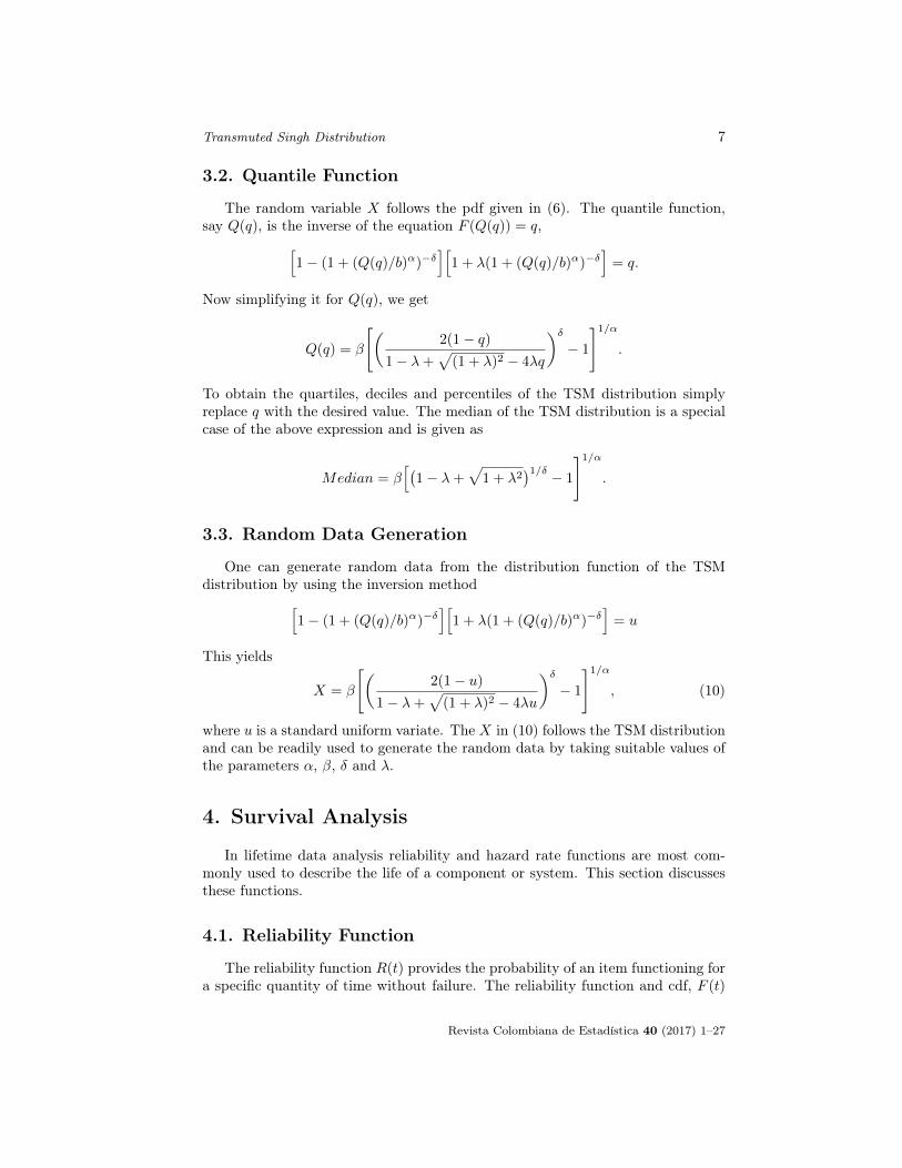
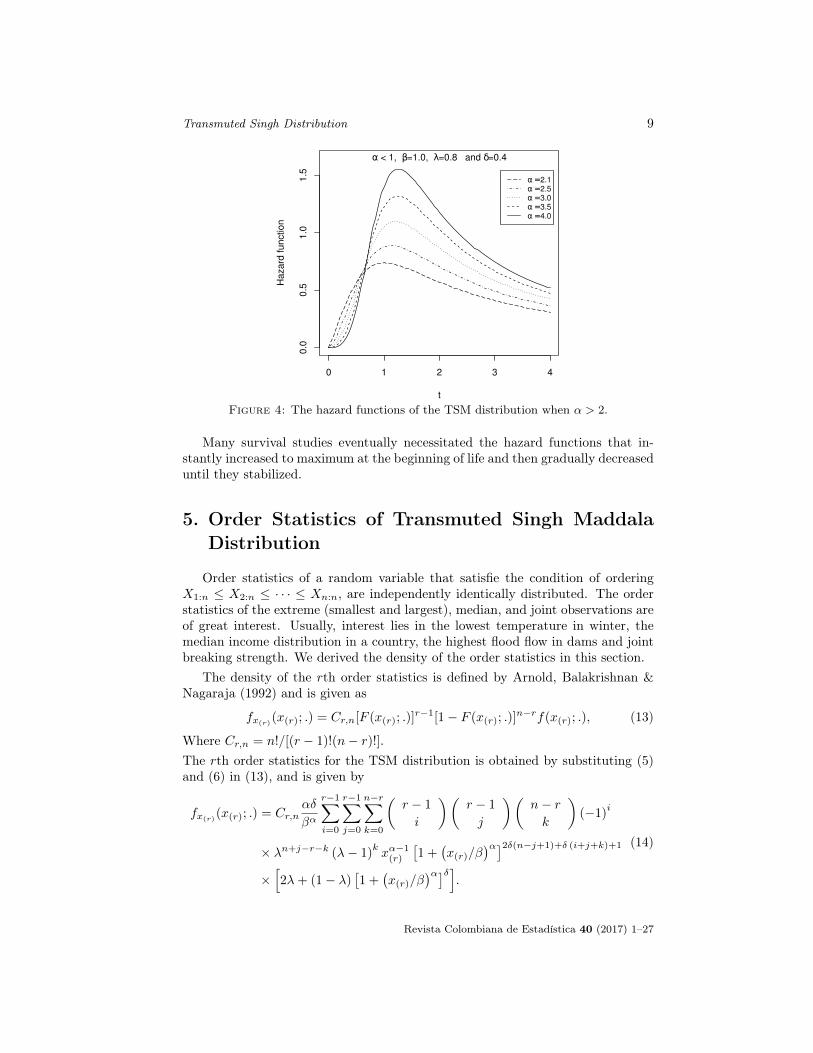
It can be observed that when α < 1, the behaviour of the hazard functiondecreases and then move constantly. When α > 2, the behavior of the hazardfunction is upside-down bathtub shaped (increasing to maximum and then de-creasing). Thus, the TSM distribution shows a decreasing, increasing, or unimodalhazard rate in specified ranges of the parametric values. The various shapes ofhazard function are presented in Figure 3 and 4 assume different combinations ofparametric values.
0 1 2 3 4 5
0.0
0.1
0.2
0.3
0.4
0.5
0.6
0.7
t
Haz
ard
func
tion
α < 1, β=1.0, λ=0.8 and δ=0.4
α=0.1α=0.3α=0.5α=0.7α=0.9
Figure 3: The hazard functions of the TSM distribution when α < 1.
Revista Colombiana de Estadística 40 (2017) 1–27
Transmuted Singh Distribution 9
0 1 2 3 4
0.0
0.5
1.0
1.5
t
Haz
ard
func
tion
α < 1, β=1.0, λ=0.8 and δ=0.4
α=2.1α=2.5α=3.0α=3.5α=4.0
Figure 4: The hazard functions of the TSM distribution when α > 2.
Many survival studies eventually necessitated the hazard functions that in-stantly increased to maximum at the beginning of life and then gradually decreaseduntil they stabilized.
5. Order Statistics of Transmuted Singh MaddalaDistribution
Order statistics of a random variable that satisfie the condition of orderingX1:n ≤ X2:n ≤ · · · ≤ Xn:n, are independently identically distributed. The orderstatistics of the extreme (smallest and largest), median, and joint observations areof great interest. Usually, interest lies in the lowest temperature in winter, themedian income distribution in a country, the highest flood flow in dams and jointbreaking strength. We derived the density of the order statistics in this section.
The density of the rth order statistics is defined by Arnold, Balakrishnan &Nagaraja (1992) and is given as
fx(r)(x(r); .) = Cr,n[F (x(r); .)]
r−1[1− F (x(r); .)]n−rf(x(r); .), (13)
Where Cr,n = n!/[(r − 1)!(n− r)!].The rth order statistics for the TSM distribution is obtained by substituting (5)and (6) in (13), and is given by
fx(r)(x(r); .) = Cr,n
αδ
βα
r−1∑i=0
r−1∑j=0
n−r∑k=0
(r − 1
i
)(r − 1
j
)(n− rk
)(−1)
i
× λn+j−r−k (λ− 1)kxα−1(r)
[1 +
(x(r)/β
)α]2δ(n−j+1)+δ (i+j+k)+1
×[2λ+ (1− λ)
[1 +
(x(r)/β
)α]δ].
(14)
Revista Colombiana de Estadística 40 (2017) 1–27

10 Mirza Naveed Shahzad, Faton Merovci & Zahid Asghar
The density of the smallest order statistic X(1) has the following form
fX(1)(x(1)) =
nαδ
βα
n−1∑i=0
(n− 1
i
)λn−i−1 (λ− 1)
ixα−1(1)
[1 +
(x(1)/β
)α]−δ(2n+i)−1×[2λ+ (1− λ)
[1 +
(x(1)/β
)α]δ].
The density of the nth order statistic, X(n) is obtained from (14) in the followingform
fx(n)(x(n); .) =
nαδ
βα
n−1∑i=0
n−1∑j=0
(r − 1
j
)(n− 1
k
)(−1)
iλjxα−1(n)
×(1 +
(x(n)/β
)α)−δ(i+j+2)−1 [2λ+ (1− λ)
[1 +
(x(n)/β
)α]δ].
The joint pdf of X(r) and X(s) (1 < r ≤ s ≤ n) for the TSM distribution is derivedby using the general expression defined by Balakrishnan & Cohen (1991). So, thejoint pdf is obtained in the following form
fX(r)X(s)(u, v) = Cr,s,n
(αδ)2(uv)α−1
β2α
s−r−1∑i=0
r+i−1∑j=0
r+i−1∑k=0
s−r−i−1∑l=0
s−r−i−1∑m=0
n−s∑t=0
×(s− r − 1
i
)(r + i− 1
j
)(r + i− 1
k
)(s− r − i− 1
l
)×(s− r − i− 1
m
)(−1)i+j+l (λ− 1)
tλk+m+n−s−t
× [1 + (u/β)α
]−δ (j+k+2)−1
(1 + (v/β)α
)−δ(l+m+t)−2δ(n−s+1)−1
×[2λ+ (1− λ) [1 + (v/β)
α]δ],
where Cr,s,n = n![(r−1)!(s−r−1)!(n−s)!] .
6. Generalized TL-Moments
The TL-moments are a worthwhile contribution to extreme values analysis.These moments, based on order statistics, describe the shape of the probabilitydistribution in a better way than conventional methods. Elamir & Seheult (2003)introduced the rth generalized TL-moments as follows
T (s,t)r = r−1
r−1∑k=0
(−1)k(
r − 1
k
)E (Xr+s−k:r+s+t) , r = 1, 2, . . . ; t, s = 0, 1, 2 . . . (15)
where T (s,t)r is a linear function of the expectations of the order statistics s and
t. The s and t are the possible trimming lowest and highest values, respectively.
Revista Colombiana de Estadística 40 (2017) 1–27
Transmuted Singh Distribution 11
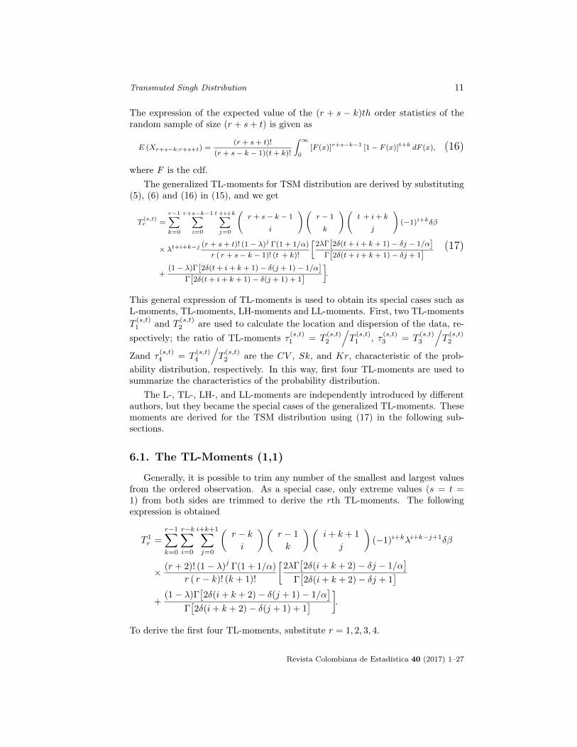
The expression of the expected value of the (r + s − k)th order statistics of therandom sample of size (r + s+ t) is given as
E (Xr+s−k:r+s+t) =(r + s+ t)!
(r + s− k − 1)(t+ k)!
∫ ∞0
[F (x)]r+s−k−1 [1 − F (x)]t+k dF (x), (16)
where F is the cdf.The generalized TL-moments for TSM distribution are derived by substituting
(5), (6) and (16) in (15), and we get
T(s,t)r =
r−1∑k=0
r+s−k−1∑i=0
t+i+k∑j=0
(r + s− k − 1
i
)(r − 1
k
)(t + i+ k
j
)(−1)i+kδβ
× λt+i+k−j(r + s+ t)! (1 − λ)j Γ(1 + 1/α)
r ( r + s− k − 1)! (t + k)!
[2λΓ
[2δ(t+ i+ k + 1) − δj − 1/α
]Γ[2δ(t+ i+ k + 1) − δj + 1
]+
(1 − λ)Γ[2δ(t+ i+ k + 1) − δ(j + 1) − 1/α
]Γ[2δ(t+ i+ k + 1) − δ(j + 1) + 1
] ].
(17)
This general expression of TL-moments is used to obtain its special cases such asL-moments, TL-moments, LH-moments and LL-moments. First, two TL-momentsT
(s,t)1 and T (s,t)
2 are used to calculate the location and dispersion of the data, re-spectively; the ratio of TL-moments τ (s,t)1 = T
(s,t)2
/T
(s,t)1 , τ (s,t)3 = T
(s,t)3
/T
(s,t)2
Zand τ(s,t)4 = T
(s,t)4
/T
(s,t)2 are the CV , Sk, and Kr, characteristic of the prob-
ability distribution, respectively. In this way, first four TL-moments are used tosummarize the characteristics of the probability distribution.
The L-, TL-, LH-, and LL-moments are independently introduced by differentauthors, but they became the special cases of the generalized TL-moments. Thesemoments are derived for the TSM distribution using (17) in the following sub-sections.
6.1. The TL-Moments (1,1)
Generally, it is possible to trim any number of the smallest and largest valuesfrom the ordered observation. As a special case, only extreme values (s = t =1) from both sides are trimmed to derive the rth TL-moments. The followingexpression is obtained
T 1r =
r−1∑k=0
r−k∑i=0
i+k+1∑j=0
(r − ki
)(r − 1
k
)(i+ k + 1
j
)(−1)i+kλi+k−j+1δβ
× (r + 2)! (1− λ)j
Γ(1 + 1/α)
r ( r − k)! (k + 1)!
[2λΓ
[2δ(i+ k + 2)− δj − 1/α
]Γ[2δ(i+ k + 2)− δj + 1
]+
(1− λ)Γ[2δ(i+ k + 2)− δ(j + 1)− 1/α
]Γ[2δ(i+ k + 2)− δ(j + 1) + 1
] ].
To derive the first four TL-moments, substitute r = 1, 2, 3, 4.
Revista Colombiana de Estadística 40 (2017) 1–27
12 Mirza Naveed Shahzad, Faton Merovci & Zahid Asghar
6.2. The L-Moments
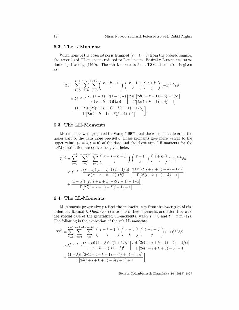
When none of the observation is trimmed (s = t = 0) from the ordered sample,the generalized TL-moments reduced to L-moments. Basically L-moments intro-duced by Hosking (1990). The rth L-moments for a TSM distribution is givenas
T 0r =
r−1∑k=0
r−k−1∑i=0
i+k∑j=0
(r − k − 1
i
)(r − 1
k
)(i+ k
j
)(−1)i+kδβ
× λi+k−j (r)! (1− λ)j
Γ(1 + 1/α)
r ( r − k − 1)! (k)!
[2λΓ
[2δ(i+ k + 1)− δj − 1/α
]Γ[2δ(i+ k + 1)− δj + 1
]+
(1− λ)Γ[2δ(i+ k + 1)− δ(j + 1)− 1/α
]Γ[2δ(i+ k + 1)− δ(j + 1) + 1
] ].
6.3. The LH-Moments
LH-moments were proposed by Wang (1997), and these moments describe theupper part of the data more precisely. These moments give more weight to theupper values (s = s, t = 0) of the data and the theoretical LH-moments for theTSM distribution are derived as given below
T (s)r =
r−1∑k=0
r+s−k−1∑i=0
i+k∑j=0
(r + s− k − 1
i
)(r − 1
k
)(i+ k
j
)(−1)i+kδβ
× λi+k−j (r + s)! (1− λ)j
Γ(1 + 1/α)
r ( r + s− k − 1)! (k)!
[2λΓ
[2δ(i+ k + 1)− δj − 1/α
]Γ[2δ(i+ k + 1)− δj + 1
]+
(1− λ)Γ[2δ(i+ k + 1)− δ(j + 1)− 1/α
]Γ[2δ(i+ k + 1)− δ(j + 1) + 1
] ].
6.4. The LL-Moments
LL-moments progressively reflect the characteristics from the lower part of dis-tribution. Bayazit & Onoz (2002) introduced these moments, and later it becamethe special case of the generalized TL-moments, when s = 0 and t = t in (17).The following is the expression of the rth LL-moments
T (t)r =
r−1∑k=0
r−k−1∑i=0
t+i+k∑j=0
(r − k − 1
i
)(r − 1
k
)(t + i+ k
j
)(−1)i+kδβ
× λt+i+k−j (r + t)! (1− λ)j
Γ(1 + 1/α)
r ( r − k − 1)! (t + k)!
[2λΓ
[2δ(t+ i+ k + 1)− δj − 1/α
]Γ[2δ(t+ i+ k + 1)− δj + 1
]+
(1− λ)Γ[2δ(t+ i+ k + 1)− δ(j + 1)− 1/α
]Γ[2δ(t+ i+ k + 1)− δ(j + 1) + 1
] ]
Revista Colombiana de Estadística 40 (2017) 1–27
Transmuted Singh Distribution 13
The LH and LL-moments can be evaluated for any value of t and s, but thepreferable value for both is upto 4.
7. Parameter Estimation by Maximum Likelihood
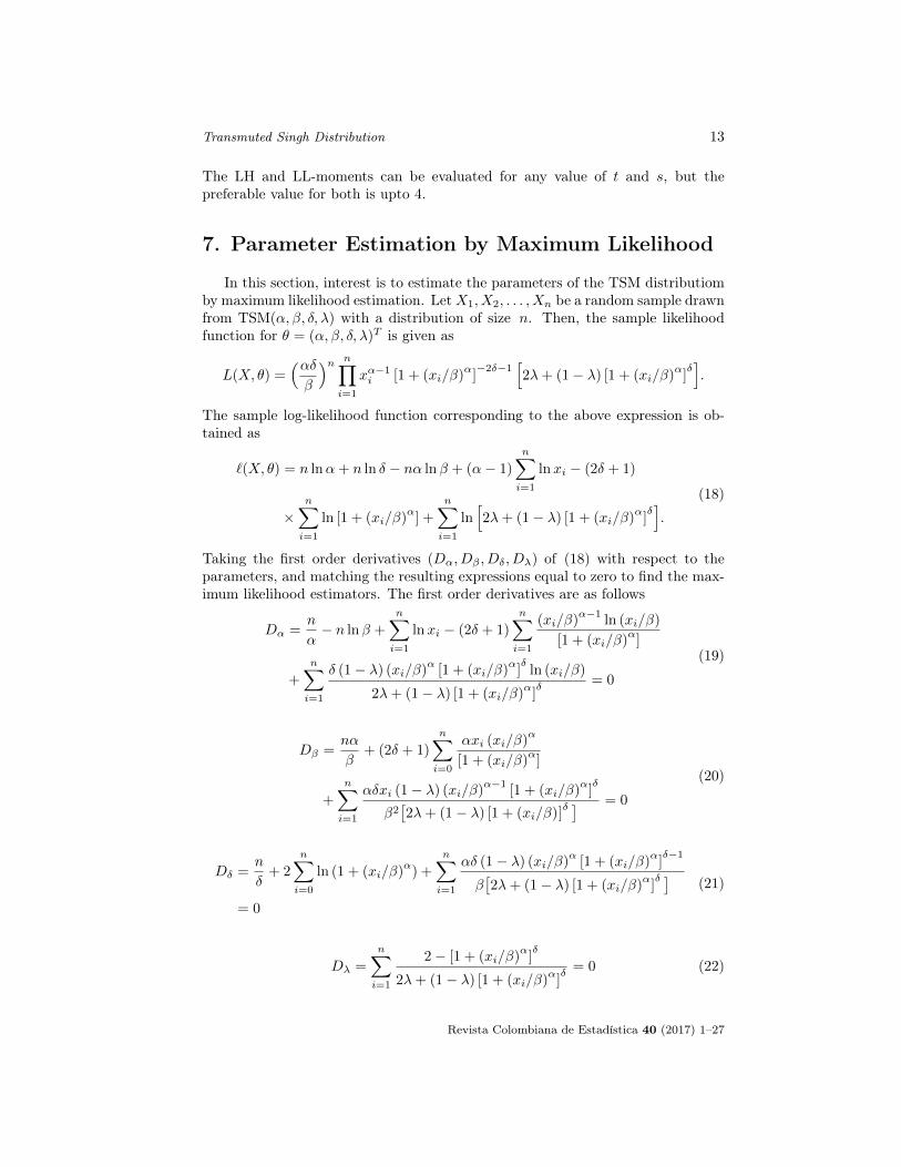
In this section, interest is to estimate the parameters of the TSM distributiomby maximum likelihood estimation. LetX1, X2, . . . , Xn be a random sample drawnfrom TSM(α, β, δ, λ) with a distribution of size n. Then, the sample likelihoodfunction for θ = (α, β, δ, λ)T is given as
L(X, θ) =(αδβ
)n n∏i=1
xα−1i [1 + (xi/β)α
]−2δ−1
[2λ+ (1− λ) [1 + (xi/β)
α]δ].
The sample log-likelihood function corresponding to the above expression is ob-tained as
`(X, θ) = n lnα+ n ln δ − nα lnβ + (α− 1)
n∑i=1
lnxi − (2δ + 1)
×n∑i=1
ln [1 + (xi/β)α
] +
n∑i=1
ln[2λ+ (1− λ) [1 + (xi/β)
α]δ].
(18)
Taking the first order derivatives (Dα, Dβ , Dδ, Dλ) of (18) with respect to theparameters, and matching the resulting expressions equal to zero to find the max-imum likelihood estimators. The first order derivatives are as follows
Dα =n
α− n lnβ +
n∑i=1
lnxi − (2δ + 1)
n∑i=1
(xi/β)α−1
ln (xi/β)
[1 + (xi/β)α
]
+
n∑i=1
δ (1− λ) (xi/β)α
[1 + (xi/β)α
]δ
ln (xi/β)
2λ+ (1− λ) [1 + (xi/β)α
]δ
= 0
(19)
Dβ =nα
β+ (2δ + 1)
n∑i=0
αxi (xi/β)α
[1 + (xi/β)α
]
+
n∑i=1
αδxi (1− λ) (xi/β)α−1
[1 + (xi/β)α
]δ
β2[2λ+ (1− λ) [1 + (xi/β)]
δ ] = 0
(20)
Dδ =n
δ+ 2
n∑i=0
ln (1 + (xi/β)α
) +
n∑i=1
αδ (1− λ) (xi/β)α
[1 + (xi/β)α
]δ−1
β[2λ+ (1− λ) [1 + (xi/β)
α]δ ]
= 0
(21)
Dλ =
n∑i=1
2− [1 + (xi/β)α
]δ
2λ+ (1− λ) [1 + (xi/β)α
]δ
= 0 (22)
Revista Colombiana de Estadística 40 (2017) 1–27

14 Mirza Naveed Shahzad, Faton Merovci & Zahid Asghar
The exact closed forms of maximum likelihood estimators are not possible, sothe estimates α, β, δ, and λ of parameters α, β, δ and λ, respectively are obtainedby analytically solving the above four nonlinear equations. Solving the nonlinearsystem of equations is conveniently possible by quasi-Newton algorithm.
Let Dθ = (Dα, Dβ , Dδ, Dλ)T be the TSM-score vector, then by definition, the
TSM-expected information for θ can be computed as Iθ = E[DθD
Tθ
]. Thus, the
elements Iθiθj = E[DθiD
Tθj
]from the matrix are derived, shown in Appendix, and
it is observed that the matrix is not singular. In particular, the diagonal elementsof the inverse Fisher information matrix can be taken to obtain the standard errorsof the parameter estimates. Under general regularity conditions, the asymptoticdistribution of
(θ − θ
)is multivariate normal N4
(0, I−1θ
). Consequently, the
approximately multivariate normal distribution for θ can be used to obtain thetwo sided confidence intervals for the parameters in θ. Furthermore, likelihoodratio (LR) statistic can be used to compare the TSM distribution with its specialmodel. Let the as consider the partition θ =
(θTi , θ
Tr
)T , where θTi = (α, β, δ), andθTr = (λ). The LR statistic to test the null hypothesis H0 : λ = 0 versus thealternative hypothesis Ha : λ 6= 0 is given by w = 2
[`(θ)− `(θ)]
, where `(θ),
and `(θ)are the estimates under the restricted and unrestricted log-likelihood,
respectively. Moreover, the sub-matrix of the full information matrix, when λ = 0coincides with the SM-information matrix. In this case, the columns of the matrixare linearly independent and none of the column is of 0s. In this case, it also leadsto a nonsingular information matrix.
8. Numerical Computations
8.1. Simulation Study
A simulation study has been carried out for two purposes: first, to investigatethe precision and accuracy of the estimates; second, to explore the impact ofsample size on estimation techniques. Keeping this in mind, we present empiricalanalysis based on simulated data; the generation of the TSM distribution canbe easily obtained through the derived result (10). The data is simulated usingthe R-language, assuming different sample sizes, n ∈ (25, 50, 100 and 200), andassuming different values of each parameter. Each sample is repeated 1000 times.For each estimate θ =
(α, β, δ, λ
), we computed the bias and the mean square
error (MSE), respectively as
Bias(θ)
=1
n
n∑i=1
(θi − θ
)
MSE(θ)
=1
n
n∑i=1
(θi − θ
)2.
Revista Colombiana de Estadística 40 (2017) 1–27
Transmuted Singh Distribution 15
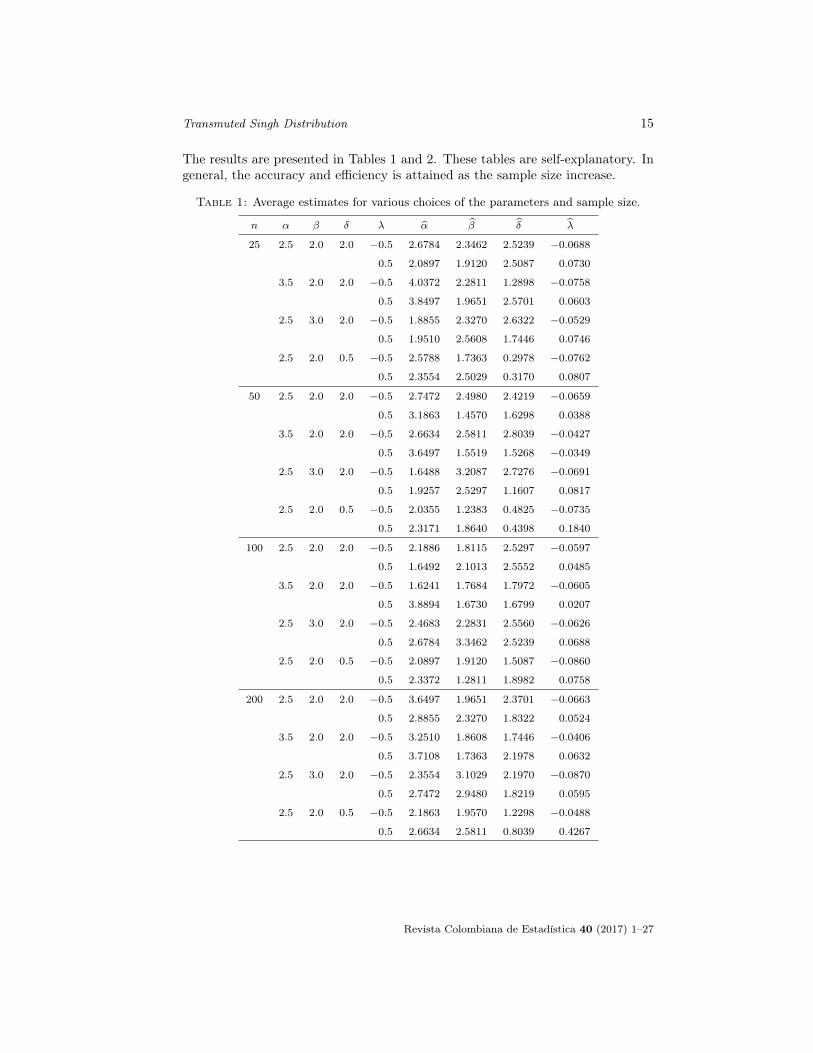
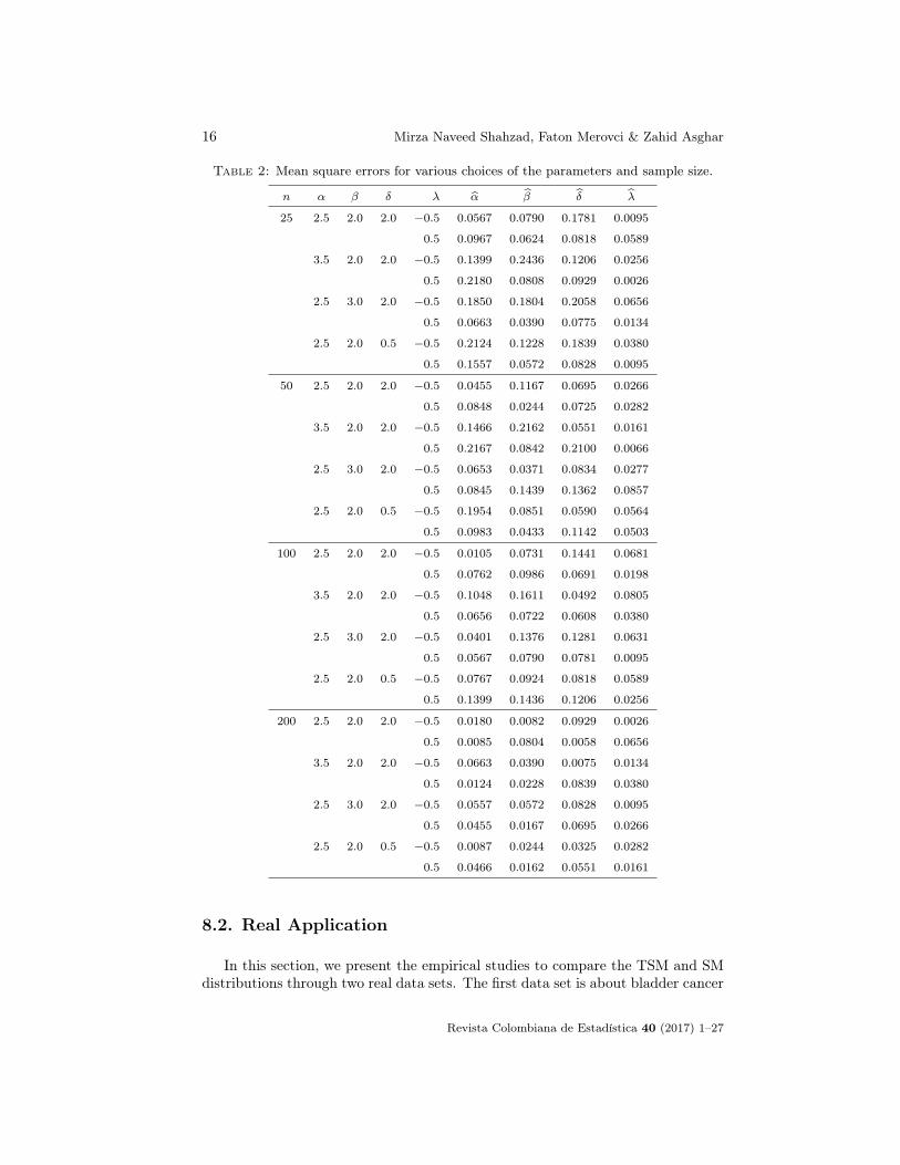
The results are presented in Tables 1 and 2. These tables are self-explanatory. Ingeneral, the accuracy and efficiency is attained as the sample size increase.
Table 1: Average estimates for various choices of the parameters and sample size.
n α β δ λ α β δ λ
25 2.5 2.0 2.0 −0.5 2.6784 2.3462 2.5239 −0.0688
0.5 2.0897 1.9120 2.5087 0.0730
3.5 2.0 2.0 −0.5 4.0372 2.2811 1.2898 −0.0758
0.5 3.8497 1.9651 2.5701 0.0603
2.5 3.0 2.0 −0.5 1.8855 2.3270 2.6322 −0.0529
0.5 1.9510 2.5608 1.7446 0.0746
2.5 2.0 0.5 −0.5 2.5788 1.7363 0.2978 −0.0762
0.5 2.3554 2.5029 0.3170 0.0807
50 2.5 2.0 2.0 −0.5 2.7472 2.4980 2.4219 −0.0659
0.5 3.1863 1.4570 1.6298 0.0388
3.5 2.0 2.0 −0.5 2.6634 2.5811 2.8039 −0.0427
0.5 3.6497 1.5519 1.5268 −0.0349
2.5 3.0 2.0 −0.5 1.6488 3.2087 2.7276 −0.0691
0.5 1.9257 2.5297 1.1607 0.0817
2.5 2.0 0.5 −0.5 2.0355 1.2383 0.4825 −0.0735
0.5 2.3171 1.8640 0.4398 0.1840
100 2.5 2.0 2.0 −0.5 2.1886 1.8115 2.5297 −0.0597
0.5 1.6492 2.1013 2.5552 0.0485
3.5 2.0 2.0 −0.5 1.6241 1.7684 1.7972 −0.0605
0.5 3.8894 1.6730 1.6799 0.0207
2.5 3.0 2.0 −0.5 2.4683 2.2831 2.5560 −0.0626
0.5 2.6784 3.3462 2.5239 0.0688
2.5 2.0 0.5 −0.5 2.0897 1.9120 1.5087 −0.0860
0.5 2.3372 1.2811 1.8982 0.0758
200 2.5 2.0 2.0 −0.5 3.6497 1.9651 2.3701 −0.0663
0.5 2.8855 2.3270 1.8322 0.0524
3.5 2.0 2.0 −0.5 3.2510 1.8608 1.7446 −0.0406
0.5 3.7108 1.7363 2.1978 0.0632
2.5 3.0 2.0 −0.5 2.3554 3.1029 2.1970 −0.0870
0.5 2.7472 2.9480 1.8219 0.0595
2.5 2.0 0.5 −0.5 2.1863 1.9570 1.2298 −0.0488
0.5 2.6634 2.5811 0.8039 0.4267
Revista Colombiana de Estadística 40 (2017) 1–27
16 Mirza Naveed Shahzad, Faton Merovci & Zahid Asghar
Table 2: Mean square errors for various choices of the parameters and sample size.
n α β δ λ α β δ λ
25 2.5 2.0 2.0 −0.5 0.0567 0.0790 0.1781 0.0095
0.5 0.0967 0.0624 0.0818 0.0589
3.5 2.0 2.0 −0.5 0.1399 0.2436 0.1206 0.0256
0.5 0.2180 0.0808 0.0929 0.0026
2.5 3.0 2.0 −0.5 0.1850 0.1804 0.2058 0.0656
0.5 0.0663 0.0390 0.0775 0.0134
2.5 2.0 0.5 −0.5 0.2124 0.1228 0.1839 0.0380
0.5 0.1557 0.0572 0.0828 0.0095
50 2.5 2.0 2.0 −0.5 0.0455 0.1167 0.0695 0.0266
0.5 0.0848 0.0244 0.0725 0.0282
3.5 2.0 2.0 −0.5 0.1466 0.2162 0.0551 0.0161
0.5 0.2167 0.0842 0.2100 0.0066
2.5 3.0 2.0 −0.5 0.0653 0.0371 0.0834 0.0277
0.5 0.0845 0.1439 0.1362 0.0857
2.5 2.0 0.5 −0.5 0.1954 0.0851 0.0590 0.0564
0.5 0.0983 0.0433 0.1142 0.0503
100 2.5 2.0 2.0 −0.5 0.0105 0.0731 0.1441 0.0681
0.5 0.0762 0.0986 0.0691 0.0198
3.5 2.0 2.0 −0.5 0.1048 0.1611 0.0492 0.0805
0.5 0.0656 0.0722 0.0608 0.0380
2.5 3.0 2.0 −0.5 0.0401 0.1376 0.1281 0.0631
0.5 0.0567 0.0790 0.0781 0.0095
2.5 2.0 0.5 −0.5 0.0767 0.0924 0.0818 0.0589
0.5 0.1399 0.1436 0.1206 0.0256
200 2.5 2.0 2.0 −0.5 0.0180 0.0082 0.0929 0.0026
0.5 0.0085 0.0804 0.0058 0.0656
3.5 2.0 2.0 −0.5 0.0663 0.0390 0.0075 0.0134
0.5 0.0124 0.0228 0.0839 0.0380
2.5 3.0 2.0 −0.5 0.0557 0.0572 0.0828 0.0095
0.5 0.0455 0.0167 0.0695 0.0266
2.5 2.0 0.5 −0.5 0.0087 0.0244 0.0325 0.0282
0.5 0.0466 0.0162 0.0551 0.0161
8.2. Real Application
In this section, we present the empirical studies to compare the TSM and SMdistributions through two real data sets. The first data set is about bladder cancer
Revista Colombiana de Estadística 40 (2017) 1–27
Transmuted Singh Distribution 17
patients, and the second data set is the Pakistani annual household expendituredata. In order to compare the two distribution models, we consider AIC (Akaikeinformation criterion), AICC (corrected Akaike information criterion), and BIC(Bayesian information criterion). The best fitted distribution for the data alwayshas the lowest value of the −2`, AIC, AICC, and BIC. Herein
AIC = 2k − 2` , AICC = AIC +2k(k + 1)
n− k − 1and BIC = −2`+ k × log(n)
where k is the number of parameters in the statistical model, n is the sample size,and ` is the maximized value of the log-likelihood function in the model underconsidered.
The first data set represents the remission times (in months) of a random sam-ple of 128 bladder cancer patients. This data set is reported in Lee & Wang (2003).Table 3 shows parameter estimations for each one of the five fitted distributionsfor this data set and the values of AIC, BIC and AICC values. The values in Table3 indicate that the TSM distribution is a strong competitor to other distributions,those are considered here.
Table 3: Estimated parameters of the TSM, SM, Beta Pareto, Exponentiated Paretoand Pareto distribution for the remission times dataset.
Model Parameter Estimate AIC BIC AICC
α = 1.4127
Transmuted β = 17.2260 827.4 838.8 827.7Singh Maddala δ = 2.2299
λ = 0.4932
α = 1.0822
Singh Maddala β = 169.7710 832.1 844.1 832.2δ = 23.3425
k = 0.0109
Beta-Pareto β = 0.0800 970.7 979.2 970.9a = 4.8049
b = 100.5023
k = 0.4722
EPareto β = 0.0800 992.2 997.9 992.3α = 4.1518
Pareto k = 0.1519 1189.3 1192.1 1189.3β = 0.0800
The variance-covariance matrix of the MLEs under the TSM distribution forthis data set is computed as
I(θ)−1 =
0.03575211 −2.162870 −0.1696611 −0.06911613
−2.16287024 173.784115 12.6916428 6.56234277
−0.16966107 12.691643 1.6940682 −0.01112940
−0.06911613 6.562343 −0.0111294 0.58391637
.
Revista Colombiana de Estadística 40 (2017) 1–27
18 Mirza Naveed Shahzad, Faton Merovci & Zahid Asghar
Thus, the variances of the MLE of α, β, δ, and λ are var(α) = 0.03575 , var(β) =
173.78411, var(δ) = 1.69406 and var(λ) = 0.58391. Therefore, 95% confidenceintervals for α, β, δ, and λ are [1.042173, 1.783376], [0, 43.0642], [0.4.781056] and[−1, 1], respectively.
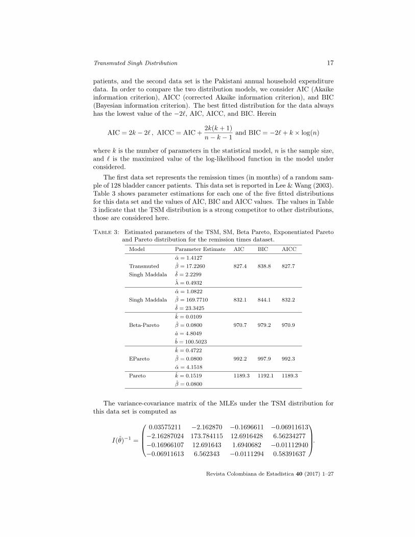
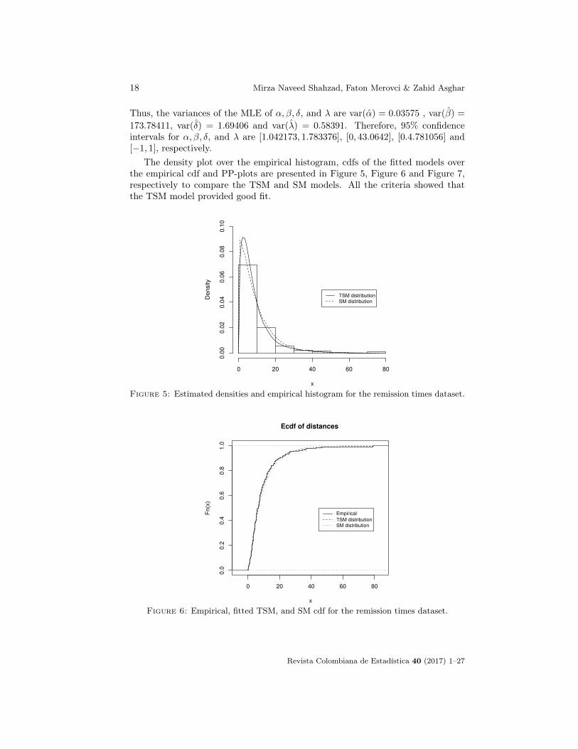
The density plot over the empirical histogram, cdfs of the fitted models overthe empirical cdf and PP-plots are presented in Figure 5, Figure 6 and Figure 7,respectively to compare the TSM and SM models. All the criteria showed thatthe TSM model provided good fit.
Histogram of x
x
Den
sity
0 20 40 60 80
0.00
0.02
0.04
0.06
0.08
0.10
TSM distributionSM distribution
Figure 5: Estimated densities and empirical histogram for the remission times dataset.
0 20 40 60 80
0.0
0.2
0.4
0.6
0.8
1.0
Ecdf of distances
x
Fn(x
)
EmpiricalTSM distributionSM distribution
Figure 6: Empirical, fitted TSM, and SM cdf for the remission times dataset.
Revista Colombiana de Estadística 40 (2017) 1–27
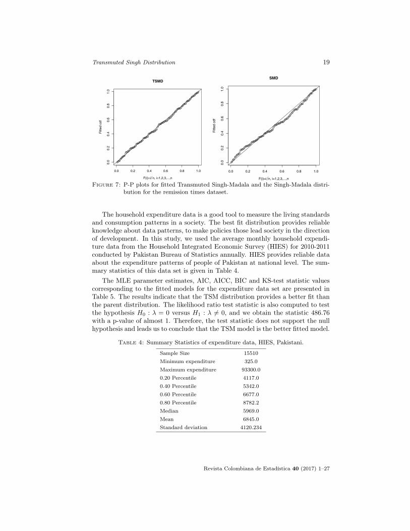
Transmuted Singh Distribution 19
0.0 0.2 0.4 0.6 0.8 1.0
0.0
0.2
0.4
0.6
0.8
1.0
TSMD
F(i)=i n, i=1,2,3,...,n
Fitt
ed c
df
0.0 0.2 0.4 0.6 0.8 1.0
0.0
0.2
0.4
0.6
0.8
1.0
SMD
F(i)=i n, i=1,2,3,...,n
Fitt
ed c
df
Figure 7: P-P plots for fitted Transmuted Singh-Madala and the Singh-Madala distri-bution for the remission times dataset.
The household expenditure data is a good tool to measure the living standardsand consumption patterns in a society. The best fit distribution provides reliableknowledge about data patterns, to make policies those lead society in the directionof development. In this study, we used the average monthly household expendi-ture data from the Household Integrated Economic Survey (HIES) for 2010-2011conducted by Pakistan Bureau of Statistics annually. HIES provides reliable dataabout the expenditure patterns of people of Pakistan at national level. The sum-mary statistics of this data set is given in Table 4.
The MLE parameter estimates, AIC, AICC, BIC and KS-test statistic valuescorresponding to the fitted models for the expenditure data set are presented inTable 5. The results indicate that the TSM distribution provides a better fit thanthe parent distribution. The likelihood ratio test statistic is also computed to testthe hypothesis H0 : λ = 0 versus H1 : λ 6= 0, and we obtain the statistic 486.76with a p-value of almost 1. Therefore, the test statistic does not support the nullhypothesis and leads us to conclude that the TSM model is the better fitted model.
Table 4: Summary Statistics of expenditure data, HIES, Pakistani.
Sample Size 15510Minimum expenditure 325.0Maximum expenditure 93300.00.20 Percentile 4117.00.40 Percentile 5342.00.60 Percentile 6677.00.80 Percentile 8782.2Median 5969.0Mean 6845.0Standard deviation 4120.234
Revista Colombiana de Estadística 40 (2017) 1–27
20 Mirza Naveed Shahzad, Faton Merovci & Zahid Asghar
I(θ)−1 =
0.00269 −3.11107 −0.00108 −0.00030
−3.11107 31447.80291 1.59301 18.18336
−0.00108 1.59301 0.00059 0.00008
−0.00030 18.18336 0.00008 0.01209
.Thus, the standard deviation (sd) of the MLE for estimates and λ are sd(α) =
0.51936, and sd(β) = 177.33528, sd(δ) = 0.02436, sd(λ) = 0.10997, respectively:therefore, 95% confidence intervals for the α, β, δ and λ are [3.83943, 4.04302],[5188.248, 5883.402], [0.80352, 0.89902] and [0.30195, 0.73304] respectively.
Table 5: Estimated parameters of TSM and SM distribution by MLE.
Model Parameter Estimate AIC BIC AICC KSα =3.9412
Transmuted β = 5535.8248 291580.6 291611.2 291580.6 0.02657Singh Maddala δ = 0.6013
λ = 0.5175
α = 3.2104
Singh Maddala β = 6262.0926 293744.2 293767.1 293744.2 0.15124δ = 23.3425
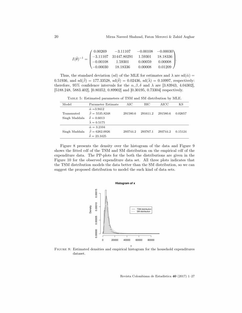
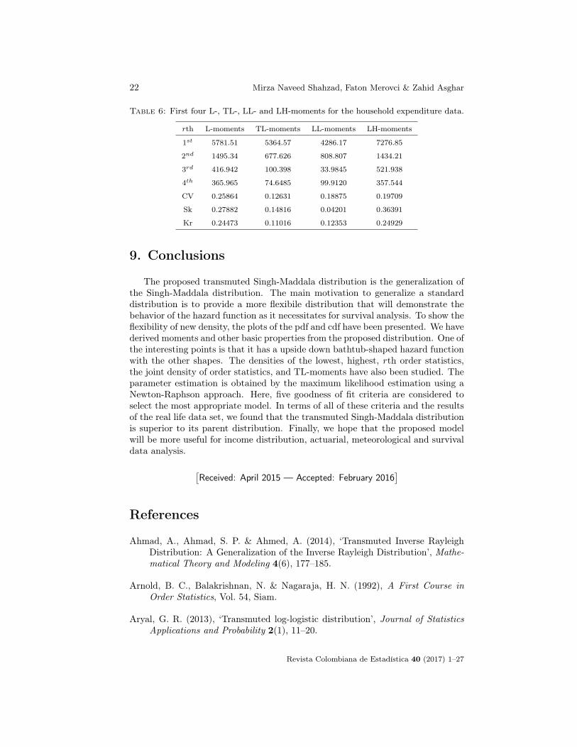
Figure 8 presents the density over the histogram of the data and Figure 9shows the fitted cdf of the TSM and SM distribution on the empirical cdf of theexpenditure data. The PP-plots for the both the distributions are given in theFigure 10 for the observed expenditure data set. All three plots indicates thatthe TSM distribution models the data better than the SM distribution, so we cansuggest the proposed distribution to model the such kind of data sets.
Histogram of x
x
Den
sity
0 20000 40000 60000 80000
0.00
000
0.00
005
0.00
010
0.00
015
TSM distributionSM distribution
Figure 8: Estimated densities and empirical histogram for the household expendituresdataset.
Revista Colombiana de Estadística 40 (2017) 1–27
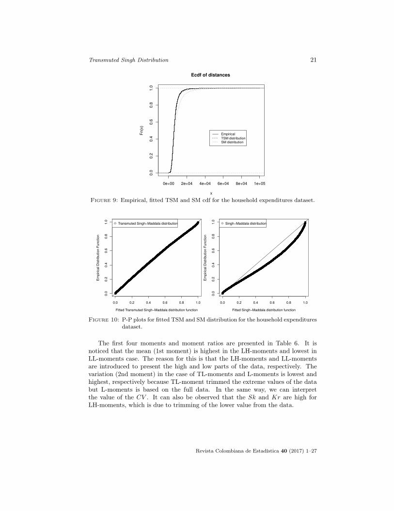
Transmuted Singh Distribution 21
0e+00 2e+04 4e+04 6e+04 8e+04 1e+05
0.0
0.2
0.4
0.6
0.8
1.0
Ecdf of distances
x
Fn(x
)
EmpiricalTSM distributionSM distribution
Figure 9: Empirical, fitted TSM and SM cdf for the household expenditures dataset.
0.0 0.2 0.4 0.6 0.8 1.0
0.0
0.2
0.4
0.6
0.8
1.0
Fitted Transmuted Singh−Maddala distribution function
Em
piric
al D
istr
ibut
ion
Func
tion
Transmuted Singh−Maddala distribution
0.0 0.2 0.4 0.6 0.8 1.0
0.0
0.2
0.4
0.6
0.8
1.0
Fitted Singh−Maddala distribution function
Em
piric
al D
istr
ibut
ion
Func
tion
Singh−Maddala distribution
Figure 10: P-P plots for fitted TSM and SM distribution for the household expendituresdataset.
The first four moments and moment ratios are presented in Table 6. It isnoticed that the mean (1st moment) is highest in the LH-moments and lowest inLL-moments case. The reason for this is that the LH-moments and LL-momentsare introduced to present the high and low parts of the data, respectively. Thevariation (2nd moment) in the case of TL-moments and L-moments is lowest andhighest, respectively because TL-moment trimmed the extreme values of the databut L-moments is based on the full data. In the same way, we can interpretthe value of the CV . It can also be observed that the Sk and Kr are high forLH-moments, which is due to trimming of the lower value from the data.
Revista Colombiana de Estadística 40 (2017) 1–27
22 Mirza Naveed Shahzad, Faton Merovci & Zahid Asghar
Table 6: First four L-, TL-, LL- and LH-moments for the household expenditure data.
rth L-moments TL-moments LL-moments LH-moments
1st 5781.51 5364.57 4286.17 7276.85
2nd 1495.34 677.626 808.807 1434.21
3rd 416.942 100.398 33.9845 521.938
4th 365.965 74.6485 99.9120 357.544
CV 0.25864 0.12631 0.18875 0.19709
Sk 0.27882 0.14816 0.04201 0.36391
Kr 0.24473 0.11016 0.12353 0.24929
9. Conclusions
The proposed transmuted Singh-Maddala distribution is the generalization ofthe Singh-Maddala distribution. The main motivation to generalize a standarddistribution is to provide a more flexibile distribution that will demonstrate thebehavior of the hazard function as it necessitates for survival analysis. To show theflexibility of new density, the plots of the pdf and cdf have been presented. We havederived moments and other basic properties from the proposed distribution. One ofthe interesting points is that it has a upside down bathtub-shaped hazard functionwith the other shapes. The densities of the lowest, highest, rth order statistics,the joint density of order statistics, and TL-moments have also been studied. Theparameter estimation is obtained by the maximum likelihood estimation using aNewton-Raphson approach. Here, five goodness of fit criteria are considered toselect the most appropriate model. In terms of all of these criteria and the resultsof the real life data set, we found that the transmuted Singh-Maddala distributionis superior to its parent distribution. Finally, we hope that the proposed modelwill be more useful for income distribution, actuarial, meteorological and survivaldata analysis.
[Received: April 2015 — Accepted: February 2016
]
References
Ahmad, A., Ahmad, S. P. & Ahmed, A. (2014), ‘Transmuted Inverse RayleighDistribution: A Generalization of the Inverse Rayleigh Distribution’, Mathe-matical Theory and Modeling 4(6), 177–185.
Arnold, B. C., Balakrishnan, N. & Nagaraja, H. N. (1992), A First Course inOrder Statistics, Vol. 54, Siam.
Aryal, G. R. (2013), ‘Transmuted log-logistic distribution’, Journal of StatisticsApplications and Probability 2(1), 11–20.
Revista Colombiana de Estadística 40 (2017) 1–27

Transmuted Singh Distribution 23
Aryal, G. R. & Tsokos, C. P. (2011), ‘Transmuted Weibull distribution: A gene-ralization of the Weibull probability distribution’, European Journal of Pureand Applied Mathematics 4(2), 89–102.
Balakrishnan, N. & Cohen, A. C. (1991), Order statistics & inference: estimationmethods, Academic Press.
Bayazit, M. & Onoz, B. (2002), ‘LL-moments for estimating low fow quantiles’,Hydrological Sciences Journal 47(5), 707–720.
Brzezinski, M. (2014), ‘Empirical modeling of the impact factor distribution’, Jour-nal of Informetrics 8(2), 362–368.
Elamir, E. A. & Seheult, A. H. (2003), ‘Trimmed L-moments’, ComputationalStatistics and Data Analysis 43(3), 299–314.
Elbatal, I. (2013), ‘Transmuted generalized inverted exponential distribution’, Eco-nomic Quality Control 28(2), 125–133.
Hosking, J. R. M. (1990), ‘L-moments: analysis and estimation of distributionsusing linear combinations of order statistics’, Journal of the Royal StatisticalSociety. Series B 52, 105–124.
Khan, M. S. & King, R. (2014), ‘A new class of transmuted inverse Weibull Dis-tribution for reliability analysis’, American Journal of Mathematical and Ma-nagement Sciences 33(4), 261–286.
Khan, M. S., King, R. & Hudson, I. (2014), ‘Characterizations of the transmutedinverse Weibull distribution’, ANZIAM Journal 55, 197–217.
Kleiber, C. & Kotz, S. (2003), Statistical Size Distributions in Economics andActuarial Sciences, Vol. 470, John Wiley & Sons.
Lee, E. & Wang, J. (2003), Statistical Methods for Survival Data Analysis, Wiley,New York.
Merovci, F. (2013), ‘Transmuted Rayleigh distribution’, Austrian Journal ofStatistics 42(1), 21–31.
Sakulski, D., Jordaan, A., Tin, L. & Greyling, C. (2014), Fitting theoretical dis-tributions to Rainy Days for Eastern Cape Drought Risk assessment, in ‘Pro-ceedings of DailyMeteo. org/2014 Conference’, p. 48.
Shahzad, M. N. & Asghar, Z. (2016), ‘Transmuted Dagum Distribution: A moreflexible and broad shaped hazard function model’, Hacettepe Journal of Ma-thematics and Statistics 45(1), 1–18.
Shao, Q., Wang, Q. & Zhang, L. (2013), A stochastic weather generation methodfor temporal precipitation simulation, in ‘20th international congress on mo-delling and simulation’, Society of Australia and New Zealand, pp. 2681–2687.
Revista Colombiana de Estadística 40 (2017) 1–27
24 Mirza Naveed Shahzad, Faton Merovci & Zahid Asghar
Sharma, V. K., Singh, S. K. & Singh, U. (2014), ‘A new upside-down bathtubshaped hazard rate model for survival data analysis’, Applied Mathematicsand Computation 239, 242–253.
Shaw, W. T. & Buckley, I. R. (2009), ‘A stochastic weather generation method fortemporal precipitation simulation: The alchemy of probability distributions:beyond Gram-Charlier expansions, and a skew-kurtotic-normal distributionfrom a rank transmutation map’, arXiv preprint arXiv:0901.0434 pp. 1–8.
Singh, S. K. & Maddala, G. (1976), ‘A function for the size distribution andincomes’, Econometrica 44, 963–970.
Wang, Q. J. (1997), ‘LH moments for statistical analysis of extreme events’, WaterResources Research 33(12), 2841–2848.
Zimmer, W. J., Keats, J. B. & Wang, F. K. (1998), ‘The Burr XII distribution inreliability analysis’, Journal of Quality Technology 30(4), 386–394.
Revista Colombiana de Estadística 40 (2017) 1–27
Transmuted Singh Distribution 25
Appendix
∂αα =− n
α2− (x/β)
α(1 + 2δ)ln[x/β]
2
1 + (x/β)α +
(x/β)2α
(1 + 2δ)ln[x/β]2
(1 + (x/β)α
)2
+(1 + (x/β)
α)−1+δ
(x/β)αδ(1− λ)ln[x/β]
2
2δ + (1 + (x/β)α
)δ(1− λ)
+(1 + (x/β)
α)−2+δ
(x/β)2α
(−1 + δ)δ(1− λ)ln[x/β]2
2δ + (1 + (x/β)α
)δ(1− λ)
− (1 + (x/β)α
)−2+2δ
(x/β)2αδ2(1− λ)
2ln[x/β]
2
(2δ + (1 + (x/β)α
)δ(1− λ))
2
∂αβ =− n
β+
(x/β)α(1 + 2δ)
(1 + (x/β)α)β− (1 + (x/β)α)−1+δ(x/β)αδ(1− λ)
β(2δ + (1 + (x/β)α)δ(1− λ))
+xα(x/β)−1+α(1 + 2δ) ln[x/β]
(1 + (x/β)α)β2
− xα(x/β)−1+2α(1 + 2δ) ln[x/β]
(1 + (x/β)α)2β2− xα(1 + (x/β)α)−1+δ(x/β)−1+αδ(1− λ) ln[x/β]
β2(2δ + (1 + (x/β)α)δ(1− λ))
− xα(1 + (x/β)α)−2+δ(x/β)−1+2α(−1 + δ)δ(1− λ) ln[x/β]
β2(2δ + (1 + (x/β)α)δ(1− λ))
+xα(1 + (x/β)α)−2+2δ(x/β)−1+2αδ2(1− λ)2 ln[x/β]
β2(2δ + (1 + (x/β)α)δ(1− λ))2
∂αδ =− 2(x/β)α ln[x/β]
1 + (x/β)α+
(1 + (x/β)α)−1+δ(x/β)α(1− λ) ln[x/β]
2δ + (1 + (x/β)α)δ(1− λ)
+(1 + (x/β)α)−1+δ(x/β)αδ(1− λ) ln[1 + (x/β)α] ln[x/β]
2δ + (1 + (x/β)α)δ(1− λ)
− (1 + (x/β)α)−1+δ(x/β)αδ(1− λ)(2 + (1 + (x/β)α)δ(1− λ) ln[1 + (x/β)α]) ln[x/β]
(2δ + (1 + (x/β)α)δ(1− λ))2
∂αλ = − (1 + (x/β)α)−1+δ(x/β)αδ ln[x/β]
2δ + (1 + (x/β)α)δ(1− λ)+
(1 + (x/β)α)−1+2δ(x/β)αδ(1− λ) ln[x/β]
(2δ + (1 + (x/β)α)δ(1− λ))2
Revista Colombiana de Estadística 40 (2017) 1–27
26 Mirza Naveed Shahzad, Faton Merovci & Zahid Asghar
∂ββ =nα
β2− x2(−1 + α)α(x/β)−2+α(1 + 2δ)
(1 + (x/β)α)β4+x2α2(x/β)−2+2α(1 + 2δ)
(1 + (x/β)α)2β4
− 2xα(x/β)−1+α(1 + 2δ)
(1 + (x/β)α)β3
+x2(−1 + α)α(1 + (x/β)α)−1+δ(x/β)−2+αδ(1− λ)
β4(2δ + (1 + (x/β)α)δ(1− λ))
+2xα(1 + (x/β)α)−1+δ(x/β)−1+αδ(1− λ)
β3(2δ + (1 + (x/β)α)δ(1− λ))
+x2α2(1 + (x/β)α)−2+δ(x/β)−2+2α(−1 + δ)δ(1− λ)
β4(2δ + (1 + (x/β)α)δ(1− λ))
− x2α2(1 + (x/β)α)−2+2δ(x/β)−2+2αδ2(1− λ)2
β4(2δ + (1 + (x/β)α)δ(1− λ))2
∂βδ =2xα(x/β)−1+α
(1 + (x/β)α)β2− xα(1 + (x/β)α)−1+δ(x/β)−1+α(1− λ)
β2(2δ + (1 + (x/β)α)δ(1− λ))
− xα(1 + (x/β)α)−1+δ(x/β)−1+αδ(1− λ) ln[1 + (x/β)α]
β2(2δ + (1 + (x/β)α)δ(1− λ))
+xα(1 + (x/β)α)−1+δ(x/β)−1+αδ(1− λ)(2 + (1 + (x/β)α)δ(1− λ) ln[1 + (x/β)α])
β2(2δ + (1 + (x/β)α)δ(1− λ))2
∂βλ =xα(1 + (x/β)
α)−1+δ
(x/β)−1+α
δ
β2(2δ + (1 + (x/β)α
)δ(1− λ))
− xα(1 + (x/β)α
)−1+2δ
(x/β)−1+α
δ(1− λ)
β2(2δ + (1 + (x/β)α
)δ(1− λ))
2
∂δδ =− n
δ2+
(1 + (x/β)α
)δ(1− λ)ln[1 + (x/β)
α]2
2δ + (1 + (x/β)α
)δ(1− λ)
− (2 + (1 + (x/β)α
)δ(1− λ) ln[1 + (x/β)
α])2
(2δ + (1 + (x/β)α
)δ(1− λ))
2
∂δλ =− (1 + (x/β)α
)δ
ln[1 + (x/β)α
]
2δ + (1 + (x/β)α
)δ(1− λ)
+(1 + (x/β)
α)δ(2 + (1 + (x/β)
α)δ(1− λ) ln[1 + (x/β)
α])
(2δ + (1 + (x/β)α
)δ(1− λ))
2
Revista Colombiana de Estadística 40 (2017) 1–27

Transmuted Singh Distribution 27
∂λλ = − (1 + (x/β)α
)2δ
(2δ + (1 + (x/β)α
)δ(1− λ))
2
Revista Colombiana de Estadística 40 (2017) 1–27


![[XLS] OF BANK MITRAS 30.04.2016.xls · Web viewDILBAG SINGH BALJINDER SINGH AMRINDER SINGH PARDEEP SINGH LAKHWINDER SINGH JASVIR SINGH MANJIT SINGH CHAMAN SHAM SUNDER SINGH PARVINDER](https://img.pdfslide.net/doc/110x75/5afca7ae7f8b9a994d8c6403/xls-of-bank-mitras-30042016xlsweb-viewdilbag-singh-baljinder-singh-amrinder.jpg)


![[G. S. Maddala, In-Moo Kim] Unit Roots, Cointegrat(BookZZ.org)](https://img.pdfslide.net/doc/110x75/55cf85dd550346484b922b2d/g-s-maddala-in-moo-kim-unit-roots-cointegratbookzzorg.jpg)


