AN ABSTRACT OF THE THESIS OF

WILLIAM P. COSART

(Name)for the Ph. D.

(Degree)

in CHEMICAL ENGINEERING presented on al/ 20 Iq')2(Daee)

Title:

(Major)

TRANSPIRATION COOLING OF A ROTATING DISK

Abstract approved:Redacted for privacy

Dr. J. G. Knudsen/Dr. C. E. Wicks

Heat transfer efficients were experimentally determined for a

transpiration-cooled rotating disk. Comparison of the experimental

results to a theoretical prediction by Sparrow and Gregg is made.

Air was injected into an air environment in this study. The

heat transfer surface used was a four-inch disk constructed of fine

mesh, porous stainless steel. Temperature of the rotating surface

was measured with an infrared radiometer, accurate to one-half to

two degrees Fahrenheit, depending on the temperature. The radio-

meter was calibrated each day by focusing on a stationary surface of

material identical to the rotating disk. Temperature of the station-

ary calibrator surface was measured with calibrated thermocouples.

The effect of both injection rate and rotational rate was in-

vestigated. Nominal injection rates of 0.35, 0.44, 0.73, and 1.04

lb/min ft2 and rotational Reynolds numbers of 19,000, 26,000, 39,000

and 51,000 were used. Within the range of variables studied, it was

found that transpiration decreased the heat transfer coefficient from

a rotating disk by as much as 80% compared to the value expected for

a non-porous disk.

Results of the experiments were correlated within approximately

ten per cent by the equation

1°g10 Nu= -0.505 ;(Hw -0.519

/ .4where Nusselt number is defined as h(\)/(0- and the injection parameter

k

is Vzw

(wv)2

The theoretical calculations of Sparrow and Gregg inadequately

predicted the experimental results because the analysis assumed

constant properties. If, however, the injection parameter Hw used

towby Sparrow and Gregg were modified with a density ratio as in-

dicated above, then the theoretical prediction and the equation

Pwabove correlate the data equally well over the range 0.3 <p-- Hw <1.3.

1973

WILLIAM PRIMM COSART

ALL RIGHTS RESERVED

TRANSPIRATION COOLING OF A ROTATING DISK

by

WILLIAM PRIMM COSART

A THESIS

submitted to

OREGON STATE UNIVERSITY

in partial fulfillment of

the requirements for the

degree of

DOCTOR OF PHILOSOPHY

June 1973

APPROVED:

Redacted for privacyof ssor of Chemical Engineering

in charge of major

Redacted for privacyProfessor of Chemical Engineering

in charge of major

Redacted for privacyHead of Department of Chemical Engineering

Redacted for privacy

Dean of Graduate School

2 0 ,Date thesis is presented /.'9 "?2

Typed by Dona J. Miller for William Primm Cosart

ACKNOWLEDGEMENTS

The author recognizes that completion of this thesis would

not have been possible without the help of many other people.

He gratefully acknowledges the assistance of the following:

Dr. James G. Knudsen and Dr. Charles E. Wicks, for assuming

advisorship for this research and encouraging me to press on to

completion, for numerous helpful suggestions during the work, and

for patient and careful reading of the manuscript while the author

was away from the campus of Oregon State University.

Dr. Eugene Elzy, for suggesting the problem originally.

Professor Emeritus Jesse Walton, for administering a Depart-

ment of Chemical Engineering which provided excellent instruction,

equipment, and financial support, thus permitting completion of

this work.

Dr. William H. Dresher, Dr. Richard M. Edwards, and Dr. Don H.

White of the College of Mines and Department of Chemical Engineering

at The University of Arizona, who permitted me to teach chemical

engineering during the past several years and never expressed doubt

in my eventual success in completing this thesis.

My colleagues in The Chemical Engineering Department at The

University of Arizona, who exuded only encouragement during my

initial attempts at teaching while still lacking a doctorate.

Dr. Richard. Williams, who gave inestimable. assistance by

preparing the drawings in this thesis, but.more-important, was

a friend, office-mate, .colleague, sounding board, encourager,

and fellow Assistant Professor who also completed his doctorate.

Mrs. Dona Miller, who typed the final manuscript, and Mmes.

Catherine Cate, Linda Tillery, and Barbara Cottrell who typed

several drafts.

Finally, I must thank Jann, Jill, and Kara, who somehow lived

through having a dad go through graduate school, and my loving wife

Nanette, who constantly encouraged me to finish this work, and who

maintained an equilibrium in our home without which neither our

children nor their father could have survived.

TABLE OF CONTENTS

Chapter Page

I INTRODUCTION 1

II THEORY AND PREVIOUS WORK 3

Previous Work 4

Flow Near A Rotating Disk 4

The Effect of Nearby Stationary Surfaces 7

Heat and Mass Transfer From a Rotating Disk 11

Transpiration Cooling 16

Theory 18

Equations of Change 18

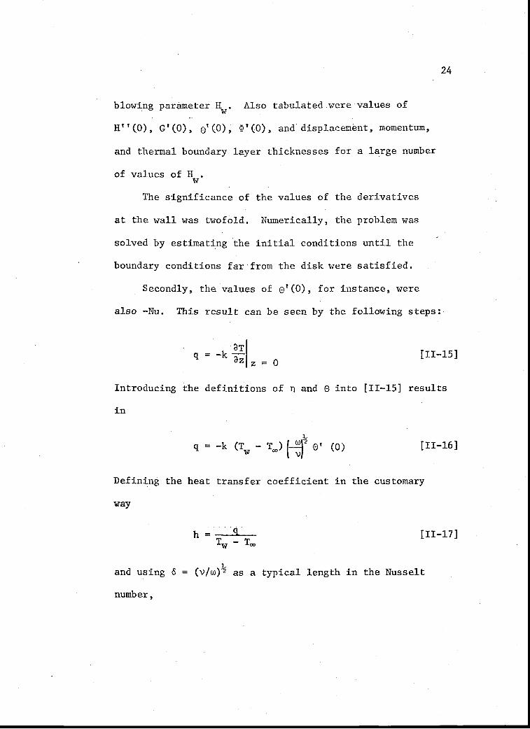
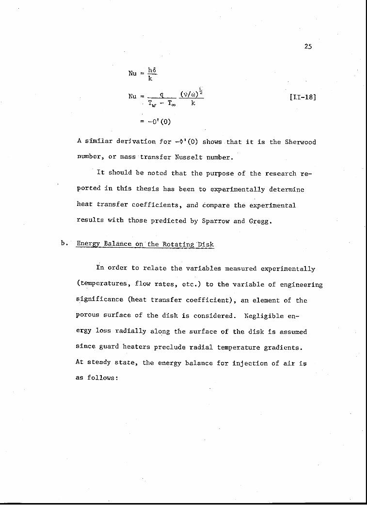
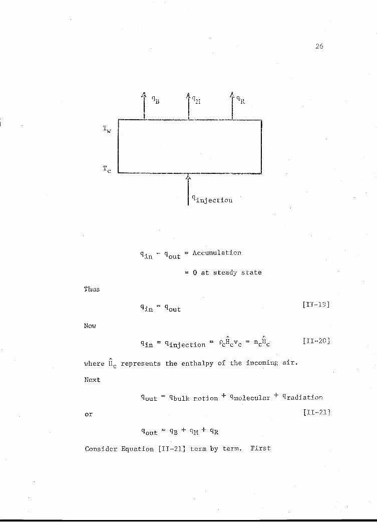
Energy Balance on the Rotating Disk 25

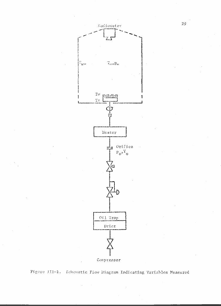
III EXPERIMENTAL EQUIPMENT AND INSTRUMENTATION 28

Source of Air 28

Rotary Union 30

Rotating Pipe 31

Heat Transfer Surface 32

Guard Heater 35

Enclosure 36

Temperature Measurement 37

Thermocouples 37

Infrared Radiometer 38

IV EXPERIMENTAL PROCEDURE 43

Calibration 43

Heat Transfer Measurement 46

V EXPERIMENTAL RESULTS 48

Experimental Data 48

Correlation of the Data 51

Discussion of Results 65

VI CONCLUSIONS 70

VII SUGGESTIONS FOR FURTHER WORK 71

BIBLIOGRAPHY 72

APPENDICES

APPENDIX A

APPENDIX B

APPENDIX C

APPENDIX D

APPENDIX E

APPENDIX F

APPENDIX C

EXPERIMENTAL RESULTS

CALCULATED RESULTS

SOURCES OF ERROR

Experimental ErrorErrors in Temperature MeasurementErrors in Flow Measurement

Uncertainty in the Value of EmissivityUncertainty in Correction for Imper-meable Area

Sum of Uncertainties

EXTRAPOLATING h TO FIND ho

DATA REDUCTION PROGRAM

LEAKAGE ANALYSIS

NOMENCLATURE

78

80

83

84

84

87

87

88

89

92

98

104

110

AppendixFigure Page

D-1 Extrapolation of.Heat Transfer. CoefficientTo Zero Injection 95

F-1 Decay of Pressure In. Sealed Piping System 106

LIST OF TABLES

AppendixTable Pave

A-1 Experimental Data 79

B-1 Calculated Results 81

B-2 Calculated Results 82

C-1 Estimated Experimental Uncertainty 86

D-1 Values of ho, eT, and. PI 94

TRANSPIRATION COOLING OF A ROTATING DISK

I. INTRODUCTION

Transpiration cooling is a means of cooling by injection of

fluid through a porous surface. During the last twenty years,

transpiration cooling has been the subject of scores of scientific

and engineering studies. High interest has been shown in the topic

from both the practical and theoretical standpoint.

Transpiration cooling is of theoretical interest in fluid

mechanics because fluid injected into a boundary layer obviously

alters the flow conditions near the wall. Since temperature and

concentration profiles are dependent on the velocity field, the

entire character of the boundary layer is affected. Moreover, the

stability of the flow, i.e. its tendency to change from laminar to

turbulent flow as well as its tendency to separate from the solid

boundary, is also affected.

The practical importance of transpiration cooling is under-

stood by visualizing the following situation: A surface is swept

by a very hot fluid, for example exhaust gases exiting through a

rocket nozzle. If the fluid is extremely hot, the mechanical

strength of the surface will be degraded, perhaps leading to

failure. If, however, the surface were porous, so that a small

amount of cool gas may be injected through it, then the surface

is cooled in two ways: First, the entering gas cools the surface

as it passes through the pores. Second, after injection into the

main stream, the coolant remains close to the surface, providing

2

an insulative blanket between the hot stream and the surface. Due

to this possibility of protecting materials exposed to very hot

environments, interest has been stimulated in studying the re-

duction of heat transfer rates (and also skin friction) by tran-

spiration in such applications as combustion chamber walls, gas

turbine blades and disks, rocket motor nozzles, hypersonic ram-jet

intakes, etc.

The particular geometry chosen for the study of transpiration

cooling reported herein is the rotating disk. The rotating disk

itself has been the subject of many investigations, for practical

as well as theoretical reasons. From the practical standpoint, the

rotating disk represents a mechanically simple model for many com-

plex items of equipment, such as turbine disks, fan blades, or

centrifugal pumps. From the theoretical standpoint, the disk is

of interest since the boundary layer induced by its rotation exhibits

three dimensional flow which can be treated by the full Navier-Stokes

equations (i.e., no terms are left out as in the two-dimensional

boundary layer equations).

Because of the extensive previous study of transpiration

cooling, and also the considerable interest in the rotating disk,

the present research stands at the confluence of two important

streams of boundary layer work. It is hoped that some light is

shed on both.

II. THEORY AND PREVIOUS WORK

A brief description of the work of others is appropriate in

order to establish the position which the present work holds in the

continuity of scientific investigation into the subjects of transpi-

ration cooling and boundary layer flow in rotating disk systems.

Such a description will also suggest areas which need further in-

vestigation, as discussed in the final chapter of the thesis.

PREVIOUS WORK will be described under the headings:

a. Flow Near a Rotating Disk

b. The Effect of Nearby Stationary Surfaces

c. Heat and /lass Transfer From a Rotating Disk

d. Transpiration Cooling

Following this summary of previous work, a more detailed

synopsis of one particular reference will be given (Sparrow and

Gregg [57]), since it formulates the theoretical foundation for

the experimental work carried out in the present investigation.

Finally, an energy balance on the rotating disk system will be

given, which provides the basis for converting the experimental

data obtained to convective heat transfer coefficients. The

THEORY portion of the chapter will thus be presented under two

headings:

a. Equations of Change

b. Energy Balance on the Rotating Disk

4

1. PREVIOUS WORK

a. Flow Near a Rotating Disk

One of the first theoretical investigations into flow

induced by a rotating disk was by von Karmen [65] in 1921.

By assuming axial symmetry and constant fluid properties

and that the radial and tangential velocities of the fluid

could be normalized into similar profiles by dividing by

the tangential velocity of the disk, the Navier-Stokes

equations were reduced to a set of ordinary differential

equations. The independent variable was a normalized

axial distance, radial distance having been eliminated.

The similarity assumption has since been verified experi-

mentally.

In 1934, Cochran [11] noted and corrected an error

in von Karman's analysis. He then re-solved the set of

equations using a different technique. Near the disk, the

dimensionless velocities were expanded in a power series

in terms of the normalized distance variable. At very

large distances from the disk, a decaying exponential

series was assumed. These solutions were then matched,

choosing the constants in the expansions so that velocities

and derivatives coincided at intermediate points.

Improvements on Cochran's solution have been given by

a number of investigators. With the advent of modern

digital computers, Ostrach and Thornton [45] recalculated

the solutions to the momentum equations using finite

difference techniques. Schwiderski and Lugt [52] con-

verted the differential equations into Volterra integral

equations, numerically solving the latter. Benton [3]

solved the time-dependent equations by a power series

expansion in wt. His solution was valid only at small t,

however, as pointed out by Homsey and Hudson [28], who

extended the work to approach steady state. They found

a single overshoot in tangential velocity which decayed

after about two revolutions of the disk.

Turbulent flow has also been studied. Assuming

velocities near the wall followed a one-seventh power

distribution, von Karmen [65] tried to calculate tur-

bulent velocity profiles. Goldstein [23] recalculated

the profiles using a logarithmic distribution. Sub-

sequently, Dorfman [19] adjusted the parameters in the

logarithmic profile to approach experimental results

more closely. More recent work by Chem and Head [8] and

Cooper [13] utilized Prandtl's mixing length theory, modi-

fied by an exponential damping factor to cause the mixing

length to disappear at the wall. In the outer portion of

the boundary layer, Cham and Head used an "entrainment

6

factor" (with an experimentally determined parameter) to

determine turbulent viscosity, while Cooper used an "inter-

mittency", the numerical value of which was borrowed from

two-dimensional boundary layer work. Both investigations

permitted reasonably accurate calculations of velocity pro-

files.

Early experimental work measured moment (i.e. drag)

coefficients and velocity profiles. Goldstein [24],

Schlicting [51], and Dorfman [19] summarized and compared

much of this work. Theodorson and Regier [61] and Gregory

and Walker [25] measured laminar velocity profiles. The

former group also measured velocities in the turbulent

regime, and determined that transition from laminar to

turbulent boundary layer occurred at Reynolds numbers

2

4112_ from 125,000 to 310,000, depending on the roughness

of the disk. Cham and Head [8] reported laminar flow up

to Re = 185,000, stable vortex formation from 185,000 to

285,000, and fully turbulent flow above 285,000. These

results gave quantitative expression to earlier, quali-

tative observations by Smith [54], who observed output

patterns from a hot-wire anemometer. Smith reported three

regimes of flow: laminar, oscillatory, and turbulent.

Theoretical investigations into the stability of

flow on a rotating disk include those of Stuart [59] and

Rogers and Lance DOI, both concluding that suction

through a porous surface tends to stabilize the boundary

layer. Without suction, Rogers and Lance reported that

flow about a disk rotating in an environment which is

also rotating can be stable only if both are rotating

in the same direction. However, the addition of suction

could provide stability even if disk and environment

rotated in opposite directions.

The effect of both suction and injection was studied

by Sparrow and Gregg [57] in a paper which formulated the

theoretical background for the experimental investigation

reported in this thesis. Working with the differential

equations of momentum and continuity derived by von Korman,

plus equations of energy and continuity of species, Sparrow

and Gregg presented solutions which included non-zero

axial velocity at the disk surface. Assuming constant

fluid properties and Pr = Sc = 0.7, velocity, temperature,

and concentration profiles as well as Nusselt numbers were

given for several values of suction and injection. A more

complete description of the equations used and results

obtained will be given under THEORY in the latter part of

this chapter.

b. The Effects of Nearb7 Stationary Surfaces

Flow in the vicinity of a rotating disk within an

8

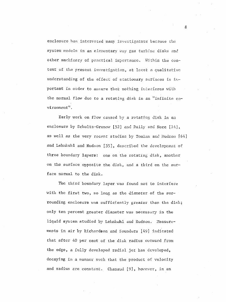
enclosure has interested many investigators because the

systet models in an elementary way gas turbine disks and

other machinery of practical importance. Within the con-

text of the present investigation, at least a qualitative

understanding of the effect of stationary surfaces is im-

portant in order to assure that nothing interferes with

the normal flow due to a rotating disk in an "infinite en-

vironment".

Early work on flow caused by a rotating disk in an

enclosure by Schultz-Grunow [52] and Daily and Nece [14],

as well as the very recent studies by Tomlan and Hudson [64]

and Lehmkuhl and Hudson [35], described the development of

three boundary layers: one on the rotating disk, another

on the surface opposite the disk, and a third on the sur-

face normal to the disk.

The third boundary layer was found not to interfere

with the first two, so long as the diameter of the sur-

rounding enclosure was sufficiently greater than the disk;

only ten percent greater diameter was necessary in the

liquid system studied by Lehmkuhl and Hudson. Measure-

ments in air by Richardson and Saunders [49] indicated

that after 40 per cent of the disk radius outward from

the edge, a fully developed radial jet has developed,

decaying in a manner such that the product of velocity

and radius are constant. Chanaud [9], however, in an

article published in 1971 measured velocity profiles

and found similarity after about ten per cent of the

disk radius away from the edge. After two to four radii,

velocities were very low and no interference with heat

transfer measurements would be expected. The box folding

the environment for the rotating disk described in the

present research is square in cross section, each edge

5.6 times the diameter of the transpired disk, thus

eliminating possible interference.

Flow patterns in an enclosure depend significantly

on axial clearance between the disk and the stationary

surface opposite the disk. When the two surfaces are

very close, the two boundary layers merge into couette

flow. For greater separation, the flow is visualized as

two individual boundary layers separated by a central core

of fluid rotating as a body at constant angular velocity.

The value of the angular velocity is some fraction of

that of the rotating disk, and depends on the clearance.

Extrapolation of the data of Daily and Nece [14] indicates

decay to zero core velocity at a separation somewhat less

than one disk diameter. Calculations by Tomlan and Hudson [63]

indicated substantial though rapidly decaying interaction at

one diameter. Mass transfer results by Kreith, Taylor, and

Chong [34] with a naphthalene disk in air indicated only a

ten per cent lowering of Sherwood number with separation of

10

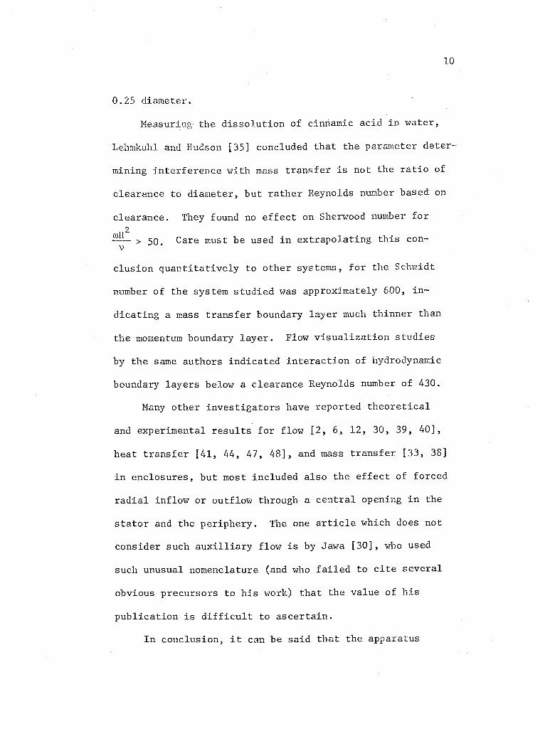
0.25 diameter,

Measuring the dissolution of cinnamic acid in water,

Lehmkuhl and Hudson [35] concluded that the parameter deter-

mining interference with mass transfer is not the ratio of

clearance to diameter, but rather Reynolds number based on

clearance. They found no effect on Sherwood number for

wH2

> 50. Care must be used in extrapolating this con-

elusion quantitatively to other systems, for the Schmidt

number of the system studied was approximately 600, in-

dicating a mass transfer boundary layer much thinner than

the momentum boundary layer. Flow visualization studies

by the same authors indicated interaction of hydrodynamic

boundary layers below a clearance Reynolds number of 430.

Many other investigators have reported theoretical

and experimental results for flow [2, 6, 12, 30, 39, 40],

heat transfer [41, 44, 47, 48], and mass transfer [33, 38]

in enclosures, but most included also the effect of forced

radial inflow or outflow through a central opening in the

stator and the periphery. The one article which does not

consider such auxilliary flow is by Jawa [30], who used

such unusual nomenclature (and who failed to cite several

obvious precursors to his work) that the value of his

publication is difficult to ascertain.

In conclusion, it can be said that the apparatus

used for the work described in this thesis was designed

to avoid interference of the surroundings with the flow

and heat transfer from the rotating disk. Clearance be-

tween the disk and the surface opposite it was greater

than ten diameters and the smallest clearance Reynolds

number was greater than seven million. Thus, regardless

of the study used to base the conclusion on [14], [34],

or [35], it is apparent that no interference is expected.

c. Heat and MasS.Transfer.Ftet a Rotating Disk

The rotating disk geometry has been the subject of

many energy and mass transfer investigations. Because

it is a model of the gas turbine disk, heat transfer has

been studied extensively, and because it provides a simple

and effective tool for measuring reaction rates, diffu-

sivities, and electrochemical transference numbers in

liquid systems (see Levich [36] for example), mass transfer

has-also received much attention. Most of the work dis-

cussed below will deal with heat transfer, since the

present investigation is limited to heat transfer in

air, with a Prandtl number of 0.7. A few mass transfer

results will be included for cases with Schmidt number

not widely different from unity since, in those cases,

the mess transport boundary layer thickness is the same

order of magnitude as the momentum transport layer. This

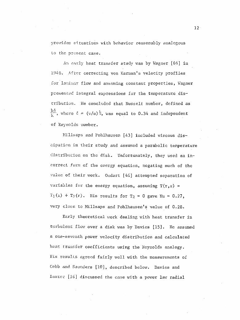
ovides situations with behavior reasonably analogous

to the present case.

An early heat transfer study was by Wagner [66] in

1948. After correcting von Karman's velocity profiles

for lami-

presented

tribution.

h67-, where

r flow and assuming constant properties, Wagner

integral expressions for the temperature dis-

He concluded that Nusselt number, defined as

6 = (v/w)k, was equal to 0.34 and independent

12

of Reynolds number.

Millsaps and Pohlhausen [43] included viscous dis-

sipation in their study and assumed a parabolic temperature

distribution on the disk. Unfortunately, they used an in-

correct form of the energy equation, negating much of the

value of their work. Oudart [46] attempted separation of

variables for the energy equation, assuming T(r,z) =

T1(z) + T2(r). His results for T2 = 0 gave Nu = 0.27,

very close to Millsaps and Pohlhausen's value of 0.28.

Early theoretical work dealing with heat transfer in

turbulent flow over a disk was by Davies [15]. He assumed

a one-seventh power velocity distribution and calculated

heat transfer coefficients using the Reynolds analogy.

His results agreed fairly well with the measurements of

Cobb and Saunders [10], described below. Davies and

Baxter [16] discussed the case with a power law radial

13

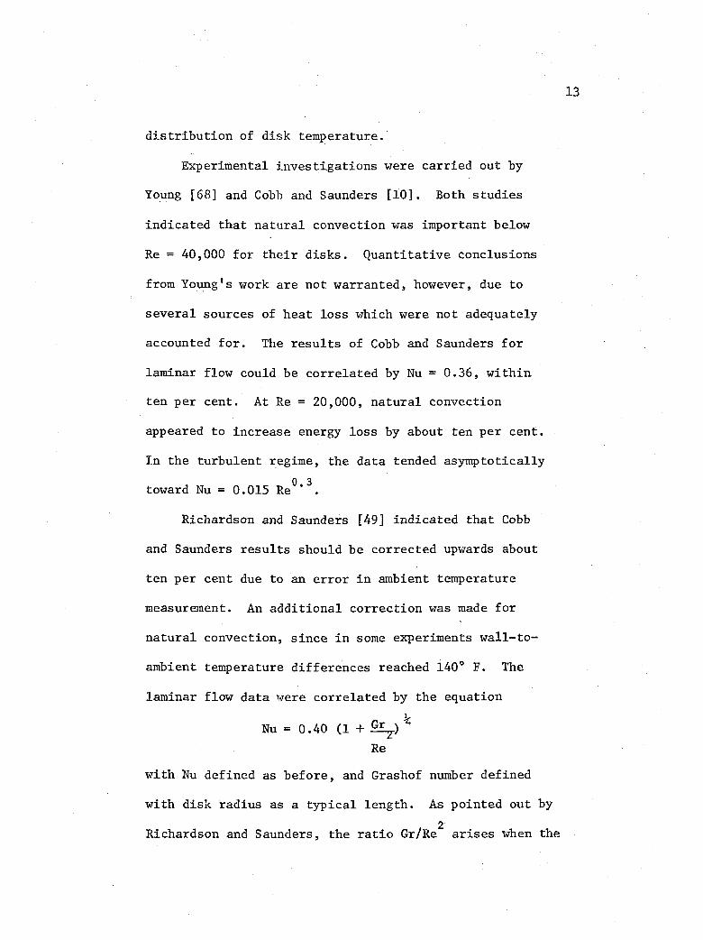
distribution of disk temperature.

Experimental investigations were carried out by

Young [68] and. Cobb and Saunders [10]. Both studies

indicated that natural convection was important below

Re = 40,000 for their disks. Quantitative conclusions

from Young's work are not warranted, however, due to

several sources of heat loss which were not adequately

accounted for. The results of Cobb and Saunders for

laminar flow could be correlated by Nu = 0.36, within

ten per cent. At Re = 20,000, natural convection

appeared to increase energy loss by about ten per cent.

In the turbulent regime, the data tended asymptotically

toward Nu = 0.015 Re0.3

.

Richardson and Saunders [49] indicated that Cobb

and Saunders results should be corrected upwards about

ten per cent due to an error in ambient temperature

measurement. An additional correction was made for

natural convection, since in some experiments wall-to-

ambient temperature differences reached 140° F. The

laminar flow data were correlated by the equation

Nu = 0.40 (1 + Gr )3/4

Re

with Nu defined as before, and Grashof number defined

with disk radius as a typical length. As pointed out by

Richardson and Saunders, the ratio Gr/Re2arises when the

14

equation of.motion is made hon-dimenSional.

Other work dealing with natural convection used the

ratio Gr/Re to correct for bouyancy effects. For example,

Fox [21] calculated a correction to the work of Hering and

Grosh [27], a study of heat transfer from a rotating cone.

With a cone half-angle of ¶/2, this reduces to the rotating

disk case. Under these circumstances, Nu as defined before

had a negligible correction for Gr/Re2= 0.01 and about a

ten per cent increase for Gr/Re2= 0.1. For Gr/Re

2= 0.5,

the correction was nearly 70 per cent. These corrections

are nearly four times those proposed by Richardson and

Saunders, the latter basing their information on experi-

ment rather than computer calculation. In either case,

the results indicate that the present research is un-

affected by natural convection, since in no case did

Gr/Re2

exceed 0.0012.

Further work concerning the rotating cone geometry

includes that of Tien [62] and Fukusako et al. [22]. Tien

considered the case of non-uniform surface temperature,

including power-law distribution and a step-change in

surface temperature. The latter case was also studied

by an analogous mass transfer experiment, using a cone

partially covered with naphthalene. Fukusako et al. con-

sidered only uniform surface temperatures, but included

15

the possibility of blowing and suction as well. Cal-

culations were carried out using power series expansions

for velocity profiles. The accuracy of the work is de-

pendent upon errors involved in truncation of the series,

but this topic was not discussed in the paper.

Other investigators used naphthalene mass transfer

experiments for rotating disk studies. Kreith, Taylor,

and Chong [34] studied both laminar and turbulent flow

with an eight inch disk. Results corroborated calculations

using the technique of Wagner [66], altering the numerical

values to account for a Schmidt number of 2.4 rather than

a Prandtl number of 0.7. The effect of placing a stationary

plane parallel to the disk was also studied (as described

previously in this review).

Recalculation of the heat transfer case using modern

computers has been carried out by Ostrach and Thornton [45],

who included the possibility of variable physical properties

(but reported results only for the case of pp = constant),

Lugt and Schwiderski [37], who converted the differential

equations to integral equations before calculating tempera-

ture profiles and Nusselt numbers, Tien and Tsuji [63], who

considered a disk rotating in an otherwise uniform flow

field directed normally to the disk, and Andrews and Riley [1],

who studied unsteady state heat transfer.

16

The work of Sparrow and Gregg [57] has been mentioned

previously, and will be discussed in more detail in a later

section.

d. Transpiration Cooling

A thorough review of the hundreds of individual con-

tributions to the widely studied field of transpiration

cooling is beyond the scope of this paper. Fortunately,

there exist already several excellent review papers, for

example Gross et al. [26] in 1961, Dewey and Gross [18]

1967, and three very broad papers in 1972 by Mills and

Wortman [42], Wortman, Mills, and Hoo [67], and Kays [31].

Gross [26] summarized the early work in two-dimensional

boundary layers with transpiration cooling. Results are

given for constant property analyses, giving velocity pro-

?,

files, 1/2CfRe2, NuxRex 2, and recovery factor as a function

of a blowing parameterp071,7

Rex2. For variable properties,PeUe

ignoring thermal diffusion and Soret effects, previous re-

sults of many investigators were brought together and

correlated with a simplified method of accounting for

foreign gas injection. The recommendation was to correct

friction coefficient and Stanton number results for air

injection with the molecular weight ratio (Nair / Ngas)1/3

17

Subsequent experiments showed this to be an over-

simplification (see Sparrow et al. [58], for instance),

but the paper served the excellent purpose of collecting

the existing information and causing additional thought

and experimentation.

The lengthy paper in 1967 by Dewey and Gross [18]

tabulated numerical results for a very wide range of

calculations for two-dimensional and axi-symmetric flow.

Included were the effect of viscous dissipation, injection,

acceleration, angle of attack, and physical property vari-

ation.

Kays [31] summarized the work of over a decade in the

Heat Transfer Laboratory at Stanford. The effect of in-

jection and suction of air into (or out of) the turbulent

boundary layer over a flat plate was studied extensively.

Results were correlated using the Prandtl mixing length

theory, modified with a simple damping function

R,= 0.4 yD

D = ytjer Y < 13+

D = 1.0 y+ 13+

where BI- depends on both the pressure gradient and the

injection rate. BI- was chosen to force the calculated

velocity profiles to match experimental ones at y+ = 80.

This technique was capable of matching friction coefficient

18

and Stanton number results even for such difficult ex-

perimental situations as step functions in injection,

step functions in pressure gradient, and combinations of

those conditions.

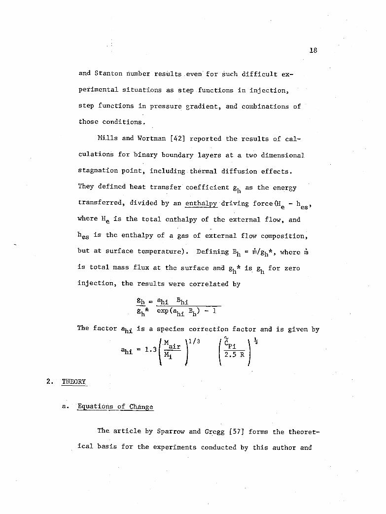
Mills and Wortman [42] reported the results of cal-

culations for binary boundary layers at a two dimensional

stagnation point, including thermal diffusion effects.

They defined heat transfer coefficient gh as the energy

transferred, divided by an enthalpy driving force(He - hes,

where He is the total enthalpy of the external flow, and

hes is the enthalpy of a gas of external flow composition,

but at surface temperature). Defining Bh = M/gh*, where

is total mass flux at the surface and gh* is gh for zero

injection, the results were correlated by

gh = ahi Bhigh* exp(ahi Bh) - 1

The factor ahi is a species correction factor and is given by

)

ahi J.= i 3 air1/3

2.5 R

2. THEORY

a. Equations of Change

The article by Sparrow and Gregg [57] forms the theoret-

ical basis for the experiments conducted by this author and

19

reported herein. It should be emphasized that this

section, which develops and transforms the equations

of change, is not original with this author, but rather

is an exposition of the work of Sparrow and Gregg.

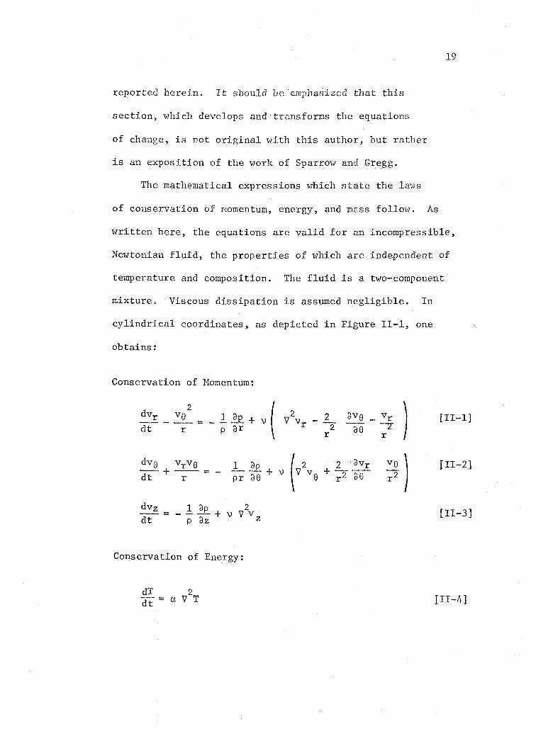
The mathematical expressions which state the laws

of conservation of momentum, energy, and mass follow. As

written here, the equations are valid for an incompressible,

Newtonian fluid, the properties of which are independent of

temperature and composition. The fluid is a two-component

mixture. Viscous dissipation is assumed negligible. In

cylindrical coordinates, as depicted in Figure II-1, one

obtains:

Conservation of Momentum:

dvr ve2

!R+ v V2v 2Dye vr [II-1]

cit r p Dr 2r

5- 7r

)

dve vrve 1 2 2 .Dvr ve [II-2]

dt r pr 0 0 r2 De r2

dvz DpV V

2v

dt p @z

Conservation of Energy:

dT 2a V Tdt

20

OJ

Figure II-1. Rotating Disk Coordinates

21

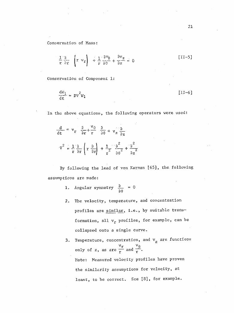
Conservation of Mass:

1 a ( Lave avzr vr 0

r Dr r DO az

Conservation of Component 1:

ari 2

dt= DV W1

In the above equations, the following operators were used:

d a v0 3

vdt r ar r DO z az

V2 D, ( ) 1 a

2 2

r ar Drr2 DO

2- +az

2

By following the lead of von Raman [65], the following

assumptions are made:

1. Angular symmetry = 0ae

2. The velocity, temperature, and concentration

profiles are similar, i.e., by suitable trans-

formation, all vr profiles, for example, can be

collapsed onto a single curve.

3. Temperature, concentration, and vzare functions

vr yeonly of z, as are 1, and T.

Note: Measured velocity profiles have proven

the similarity assumptions for velocity, at

least, to he correct. See [8], for example.

22

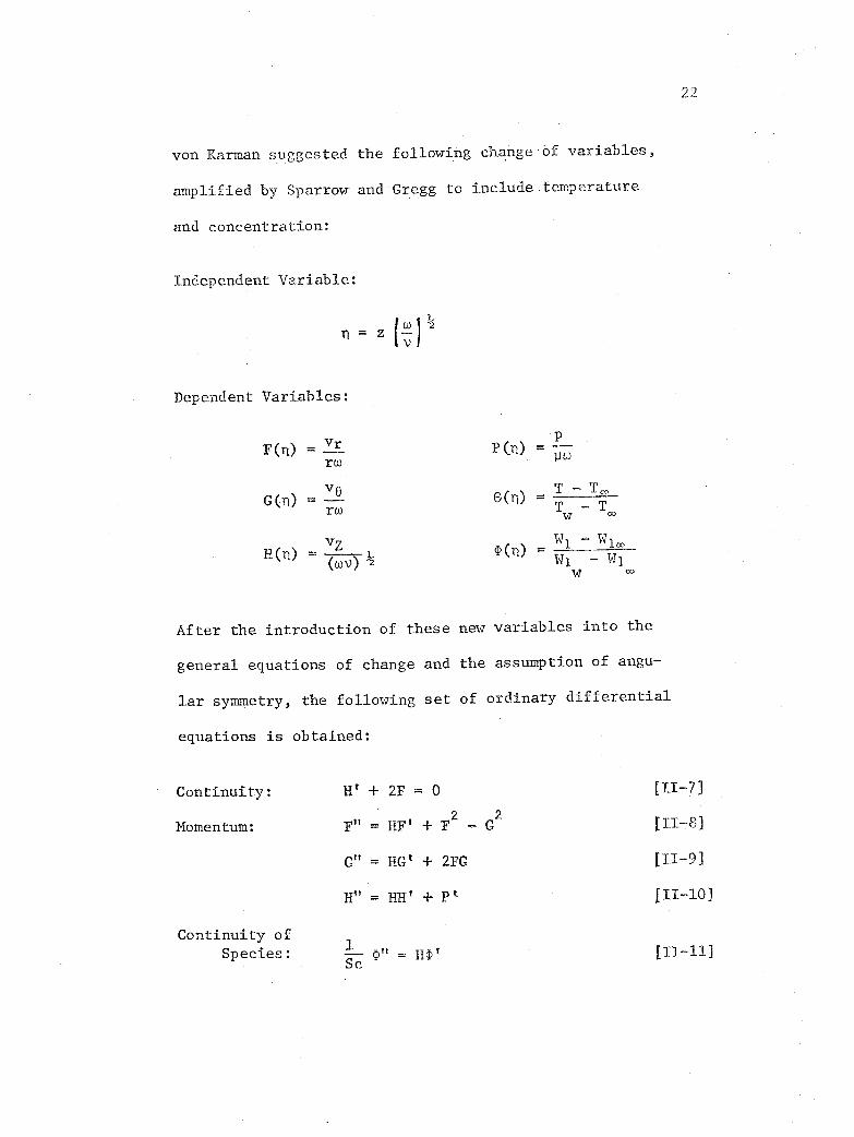
von Karmen suggested the following change of variables,

amplified by Sparrow and Gregg to include temperature

and concentration:

Independent Variable:

n=

Dependent Variables:

F =yr

rw

voG(n) =

rw

vZH(n) = 1/2

P (n) = 12--"Ito

001) =T T,T Tw cc

) W1 W1.W1 W1

After the introduction of these new variables into the

general equations of change and the assumption of angu-

lar symmetry, the following set of ordinary differential

equations is obtained:

Continuity: Ht + 2F = 0 [II-7]

Momentum: F" = HF + F2

- G2

[1178]

G" = HG' + 2FG [II-9]

Tr' Hilt + Pt [II-10]

Continuity of1

Species: 1)" = Hsic [II-11]

Sc

32

LCJ ball bearings attachecEto 1/2" thick steel plates. It was

driven through a pulley and fan belt by a 1/2 horsepower DC motor.

Constant speed was assured by a General Electric Statotrol speed

controller. Rotational rate was measured with a Strobotac (Gen-

eral Radio), calibrated before each measurement. Accuracy of the

Strobotac is reportedly 1%.

4. HEAT TRANSFER SURFACE

The porous surface consisted of thin, fine-mesh stainless

steel wire cloth. The material was 0.005 inch thick Poromesh

(Bendix Corporation) 200 x 1400 mesh. It was cut to a diameter

somewhat larger than the heat transfer area, then crimped by

forcing it into a mold exactly the same dimensions as the alu-

minum cup over which it was placed. The wire cloth was then

fastened to the cup with epoxy adhesive around the outside edge.

Within the cup was placed an insulating thickness of transite.

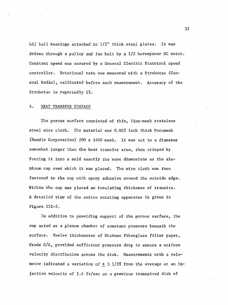
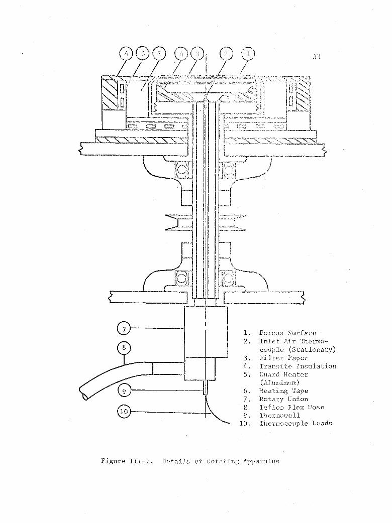
A detailed view of the entire rotating apparatus is given in

Figure 111-2.

In addition to providing support of the porous surface, the

cup acted as a plenum chamber of constant pressure beneath the

surface. Twelve thicknesses of Whatman Fiberglass filter paper,

Grade G/K, provided sufficient pressure drop to ensure a uniform

velocity distribution across the disk. Measurements with a velo-

meter indicated a variation of + 3 1/2% from the average at an in-

jection velocity of 1.4 ft/sec on a previous transpired disk of

11

1. Porous Surface2. Inlet Air Thermo-

couple (Stationary)3. Filter PaperL. Transite Insulation5. Guard Heater

(Aluminum)6. Heating Tape7. Rotary Union8. Teflon Flex Hose9. Thermowell

10. Thermocouple Leads

Figure 111-2. Details of Rotating Apparatus

.34

essentially the same design as the new disk. ,:ince 0.3 ft/s

was the highest injection. velocity used in the heat-transfer ex-

periments, actual velocity variation across the disk was no greater

than 3 1/2%.

Further indication of both uniformity with respect to radial

distance and symmetry, with respect to angular displacement, were

several measurements made with the infrared radiometer. With

heated air passing through the stationary disk, temperature was

measured at the center and at a fixed radius (near the edge of the

disk) at four angular positions, displaced 7/2.

All readings were within 0.7°F, or approXimately within the

meter's inherent accuracy at that particular temperature. Actual

readings were (°F):

center (before) 180.0

edge 180.4, 179.8, 180.0, 180.0, 179.9 (repeat of first point)

center (after) 179.7

Similar measurements made at other times gave comparable results.

An attempt was made to measure the emissivity of the porous

surface, using the method described in references [20] and [60].

However, the measurement was not successful because the accuracy

of the calculations depend upon the accuracy of the temperature

difference (Tc

Tw). For all runs tried with a stationary disk,

the largest value of (Tc Tw) was 10°F (for one run) and the other

values were 4-8°F. Since the accuracy of the instrument was as-

certained to be + 0.5 to + 2°F (see Appendix C, SOURCES OF ERROR

35

the reason for the failure of this technique for measuring emis-

sivity is apparent.

Because this measurement was not successful, a value had to be

assumed for emissivity, with a suitable allowance made for the un-

certainty this caused in subsequent calculations. (See Appendix C.)

The value assumed was 0.3, a value measured by Elzy [20] for the

same type of material made by the same manufacturer.

5. GUARD HEATER

To minimize heat losses from the surfaces of the cup other

than the porous disk, a guard-heater was placed around it. The

guard heater consisted of 3/8-inch of aluminum with a heating

tape and insulation around the outside diameter. The inside di-

ameter of the vertical face of the heater was 1/4-inch greater

than that of the cup, allowing 1/8-inch clearance. Thermocouples

were used to monitor the temperature of the inside surface of the

heater. Power to the heating tapes was supplied by a variable

transformer allowing the guard heater temperature to be adjusted

so that the disk surface showed no radial variation in temperature.

Axial heat losses from the edge of the porous surface were

minimized by a piece of transite attached to the top of the guard

heater. The transite was carefully placed approximately 1/32-inch

below the disk in order for minimal interference with the boundary

layer leaving the rotating surface. The inside diameter of the

transite was 4.125 inches, compared to 3.90 inches for the porous

disk. This left a thin ring at the outside diameter of the cup

exposed directly to the. surroundings and.not insulated by the

transite. This thin, nonporous ring was thus 10.6% of the total

surface exposed and required a correction to be applied to the

heat transfer data. (See EXPERIMENTAL RESULTS.)

6. ENCLOSURE

In order to protect the boundary layer induced by the rotation

of the disk from external convection currents, an enclosure 22" x

22" x 40" was placed around the apparatus.

The interior sides (except for the lower two inches) and bottom

of the enclosure were solid, thus preventing air currents or light

from entering. These surfaces were painted flat black.

While the lower two inches of the sides and the top of the

enclosure were permeable to air, they still shielded the interior

of the enclosure from convection currents in the room. The lower

two inches of the sides were covered with fiberglass, about one-

half inch thick. The fiberglass was below the line-of-sight of

the heat transfer surface. Over the top of the enclosure were

placed three thicknesses of black cloth. This covering and the

fiberglass prevented all visible radiation from entering the box

(important for the infrared temperature detector, as discussed

below), while still permitting the flow induced by the rotating

disk (including air injected through the porous surface) to enter

and leave the immediate environment.

37

7. TEMPERATURE 111ASUREMENT

a. Thermocouples

All temperatures measured, except that of the rotating disk

surface, were determined by calibrated iron-constantan thermocouples,

using a Doric integrating digital voltmeter. The voltmeter was

checked to 1 uv each day against a specially aged and stable zener

diode, which was an integral component within the instrument. The

voltmeter was considered accurate to at least 3 pv (0.1°F).

An ice bath, using tap water ice and deionized liquid water

and constructed in accordance with Aerospace Recommended Practice

691 [55], was used as a reference temperature for the thermocouple

measurements.

Switching between thermocouples was accomplished by a Leeds

and Northrup Type 31, 16-position, low noise selector switch. Low

thermal solder was used to connect wires to the switch. Also, it

was placed in an insulated container to prevent convection currents

in the room from causing thermal gradients in the switch.

The iron-constantan thermocouple wire had been previously cali-

brated in an oil bath against a platinum resistance thermometer.

For the calibration, a Leeds and Northrup K-3 Potentiometer was

used to measure the emf of the thermocouple, with an ice bath for

the reference junction. The potentiometer reading was repeatable

within 1 pv (1/30°F). Samples from the beginning and end of a

500 ft. reel of 40 gauge duplex wire (teflon-insulated in a fiber-

38

glass sheath) were found to give calibration curves identical within

1/30°F. Since all thermocouples used were from the same reel, it

was assumed they were of.uniform composition and had identical

calibrations.

b. Infrared Radiometer

The temperature of the porous surface was measured with a

Spartan infrared radiometer manufactured by Irtronics, Inc.,

Stamford, Connecticut. The instrument was focused visually on

the surface where the temperature was to be measured. At 40

inches, its field of view was a circle 0.75 inch in diameter.

The lead sulfide infrared detector was sensitive to wavelengths

from 1.9 to 2.9 microns. The instrument was connected to a con-

stant voltage transformer to avoid direct connection to line voltage

and to stabilize its power source.

To obtain the sensitivity and range required, it was necessary

to modify the bias on the lead sulfide detector from the value set

by the manufacturer. The emissivity correction was set at "zero"

(lowest possible emissivity), and the bias was set at 75 volts.

This permitted measurement of temperatures in the range 125°F to

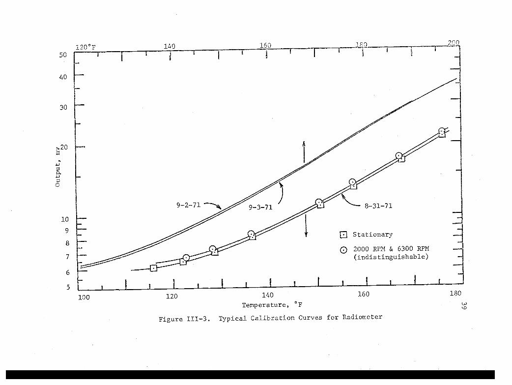
200°F. As illustrated by typical calibration curves given in

Figure 111-3, sensitivity varied from about 0.1 my / °F at 130°F to

about 0.6 my / °F at 180°F. The instrumentation output, 0-50 mv,

was transmitted by shielded cable to a second Doric integrating

digital voltmeter.

50

40

30

20E

4-3

C

10

9

8

7

6

5

120°F 1A0 160 2,00

9-2-71

0 2000 RPM & 6300 RPM(indistinguishable)

100 120 140

Temperature, °F

160

Figure 111-3. Typical Calibration Curves for Radiometer

180

Calibration of the radiometer was effected by aiming it at a

two-inch diameter stationary disk made of porouS material from the

same lot as the rotating disk. This disk was mounted in a corner

of the enclosure during calibration only, then removed before a

rotational run was started.

The stationary calibration disk was the same distance from the

radiometer as the rotating disk (40 inches). It, too, had a guard

heater wrapped with a heating tape regulated by a variable trans-

former. Spot welded to the underside of the disk were three thermo-

couples, one at the center, the other two approximately 3/8" and

1/2" from the center in opposite directions. These thermocouples

were between the porous stainless steel cloth and 12 thicknesses

of filter paper used to make the flow uniform. The flexible tef-

lon hose normally connected to the rotary union was connected to

the calibrator for a calibration run. The power to the guard

heater was adjusted to make the disk isothermal, as indicated by

the three thermocouples.

Temperature was measured by the radiometer by comparing the

infrared radiation emanating from the target to that coining from

the interior of the instrument. Therefore, it was important to

maintain a constant internal temperature, especially for targets

near room temperature. Two steps were taken to maintain the in-

terior at a constant temperature. First, cooling water was cir-

culated through the jacket of the instrument at the rate of ap-

proximately ten gallons per hour. The source of the water was a

41

constant temperature bath (Forma Scientific Corporation), regulated

at 70 + 0.1°F. Second, .the instrument was allowed to warm up at

least 24 hours before data were taken. During the major period of

data acquisition, the instrument was never turned off.

The infrared radiOmeter was equipped with a telescopic sight

to allow visual aiming through the same lens which received the

infrared signal. By aiming at a 1/16"-diameter source of light

and comparing visual signal with electronic output, it was dis-

covered that the visual aiming point was displaced appro:Umately

1/4" (at 40 inches from the lens) from the center of the infrared

aiming point. Therefore, all visual sighting had to compensate

for this displacement.

Since the detector was sensitive to all radiation it received

of appropriate wavelength, it was considered necessary to avoid

any direct or reflected light in the room. For this reason, the

enclosure was painted flat black inside, all cracks were sealed,

and the top was covered with three thicknesses of black cloth to

prevent light from entering.

It was found that the instrument was sensitive to mechanical

vibration. Hence, it was necessary to mount the radiometer sepa-

rately from the enclosure, since the enclosure was vibrated slightly

by the motor, belt, pulley, etc. The instrument was bolted to a

1/4" steel plate which in turn was mounted on two parallel rails.

42

The rails were supported at one end by a wall bracket, at the

other by a three-inch diameter stainless steel pipe running from

floor to ceiling (with cellulose sponges at top and bottom to

dampen vibrations). The rails permitted the instrument to slide

from the center of the box, over the rotating disk, to one corner,

over the stationary disk used for calibration.

43

IV. EXPERIMENTAL PROCEDURE

The experimental procedure used to acquire data is described

below in two parts: the procedure used to calib--ate the infrared

instrument, and the procedure used to determine heat transfer from

the transpired rotating disk.

1. CALIBRATION

Since earlier experimentation with the infrared radiometer had

shown its calibration curve of millivolts output versus temperature

to vary somewhat from day to day, it was considered necessary to

obtain a new calibration on each day of operation. Variation from

one day to the next was lessened by leaving the power to the instru-

ment on. (Figure 111-3 illustrates the shift encountered from one

day to the next.) The instrument was always warmed up at least

24 hours before taking any data. Variation of the calibration

on a given day was found to be negligible.

Before each day's operation, the air compressor surge tank was

drained of any water or oil accumulated from previous days. After

putting the calibrator in place in one corner of the enclosure,

the flexible teflon hose leading from the air heater was attached,

the air heater and guard heater were turned on at a level appro-

priate for the lowest temperature required for calibration, and

the air valve opened to allow approximately 0.1 lb/min to flow

through the two-inch calibrator disk. During waLm-up, the ice

44

bath was filled with cracked ice and distilled water, the radio-

meter was placed directly above the calibrator, and the enclosure

was carefully checked for light leaks. After about 1 1/2 hours,

the calibrator was usually isothermal and steady.

Before a reading was taken for the calibration curve, the

guard heater was adjusted so that the range of the three thermo-

couples attached to the underside of the 0.005-inch thick porous

stainless steel surface was less than five microvolts. Usually

the variation was less than four microvolts, i.e., the average

reading was + 2 pv. This range corresponds to the average tem-

perature + 0.07°F.

When the disk was determined to be isothermal, thermocouple

readings were taken. Radiometer readings were taken over a one

to two minute period, then the thermocouple readings were checked.

The average temperature never changed significantly (more than two

or three microvolts).

The radiometer output was led to a Doric integrating digital

voltmeter via a shielded cable. The signal was not absolutely

steady, but had considerable electronic noise which was not fil-

terable with a one or ten microfarad capacitor across the terminals

of the voltmeter. Readings were recorded as the maximum and mini-

mum digital display observed (repetition rate about one per second)

over a period of one to two minutes read to the nearest 0.01 milli-

volt. The average reading was then taken as the mean of the extremes.

While a better averaging method might have been used, it was

45

felt that any gain in accuracy would be insignificant compared

to the inherent accuracy of the instrument. To illustrate: at

the lowest temperature used the maximum and minimum were typically

1 1/2 to 2 1/2°F above and below the mean. At higher temperatures,

the interval was typically +1/2 to 1°F. It is the author's personal

judgement that the true mean must surely lie within one-half of the

extreme range. In other words, at the lowest temperatures, the true

mean was within 3/4 to 1 1/4°F of the value reported, while at higher

temperatures it was within 1/4 to 1/2°F. Further discussion of the

accuracy of the radiometer is found in Appendix C.

As mentioned in the description of the infrared instrument under

EXPERIMENTAL EQUIPMENT AND INSTRUMENTATION, the radiometric readings

were affected by vibration. While the special mounting described

earlier dampened this effect materially, some residual effect re-

mained. In order to assure that the calibration was made under the

same conditions as the subsequent heat transfer measurements, the

rotating disk was revolved at about 2000 RPM to provide vibrations

typical of operating conditions. Previous measurements had shown

negligible difference from 2000 to 6000 RPM, but usually 2-5%

difference in millivolt readings between stationary and 2000 RPM.

(Figure 111-3 illustrates the effect of vibration on the calibra-

tion curve.) Thus calibration readings were made with the rotating

disk moving while the radiometer was aimed at the stationary cali-

brator disk.

Calibration points were taken every 6-8°F from 125-140°F and

46

every 10-12°F from 140-200°F. It usually required about 30 minutes

for new air heater and guard heater settings to bring about steady,

isothermal readings on the calibrator disk. Readings were taken at

lowest temperatures first, then at successively higher temperatures.

Five to six hours were required to complete a calibration.

2. 'HEAT TRANSFER MEASUREMENT

After completing a calibration curve, the flexible hose was

immediately connected to the rotary union and air flow and heat

were adjusted to the values needed for the first rotational run.

During the warm-up period of three and one-half to six hours, other

changes in experimental set-up were made. For example, the cali-

brator was removed and replaced with a plywood dummy to keep light

and air currents out. Four theLmocouples (those measuring Tc, Too,

and two guard heater temperatures) were attached to a 16-point

recorder (altered to scan the four points repeatedly). The re-

corder was not used for any final measurement, but was very helpful

in observing the approach to steady state. Other preparations

during warm-up included moving the radiometer to its position over

the rotating disk, checking for light leaks, etc. Rotation was

started one to two hours after air flow.

As the recorded temperatures approached steady state, infrared

readings were also recorded (by hand) and trends observed. Each

infrared reading consisted of a maximum and a minimum, as discussed

under CALIBRATION. Readings were taken:

47

(a) at the.center of the disk;

(b) at theedge-ef.the disk (edgeof.the. 3/4"

field of view was within about .1/4' of the

edge of the .porous- disk), and

(c) at the center of the disk.

AdjuStments were made in the guard heater to cause tenter-

edge-center readings to coincide as nearly as possible. With

all temperatures close to 130°F, the indicated variation across

the disk was often 0.5°F. All other runs had apparent variations

of 0.3°F or less. Since these variations were less than the ac-

curacy claimed for the instrument, the disk was taken to be iso-

thermal at the average temperature observed.

When the disk appeared to be isothermal and temperatures

appeared to be steady, the thermocouples were disconnected-from

the recorder and reconnected to the thermocouple switch. After

all thermocouple readings were taken, the infrared readings were

taken again to make certain that they had not changed. If all

readings remained essentially unchanged 10-15 minutes later,

that run was concluded and a new injection rate or a new ro-

tational rate was started, steady state achieved, etc. After

the first run on a given day, successive runs required from one

and one-half to three hours to come to steady .state.

48

V. EXPERIMENTAL RESULTS

The results of the research carried out are described under

the following sections.

1. Experimental Data, which describes how the raw data

are presented and how heat transfer coefficients were

calculated and corrected;

2. Correlation of the Data, which describes how previous

investigators have correlated both transpiration and

non-transpiration heat transfer data and how the present

data are put into similar correlations;

3. Discussion of Results, which comments on the scatter

of the data around the correlations and compares the

present data to theoretical predictions and to previous

data for other systems.

1. EXPERIMENTAL DATA

The data collected are presented in Appendix A. This tabulation

represents the data as taken during experimental runs and converted

directly to calculated values by previously obtained calibration

charts (see EXPERIMENTAL EQUIPMENT AND INSTRUMENTATION for a de-

scription of the calibration curves used and their accuracy).

As discussed in THEORY'AND.PREVIOUS WORK, temperature differ-

ences and flow rates are converted to heat transfer coefficients

by the equation

h=nw C .(T Tv7),- oepew c

TtiT -T0

4Tx,7

49

[V-1]

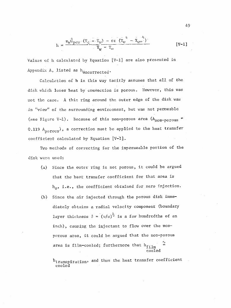
Values of it calculated by Equation [V-1] are also presented in

Appendix A, listed as h-uncorrected'

Calculation of h in thiS way tacitly assumes that all of the

disk which loses heat by convection is porous. However, this was

not the case. A thin ring around the outer edge of the disk was

in "view' of the surrounding environment, but was not permeable

(see Figure V-1). Because of this non-porous area (Anon-porous

0.119 Apterous)' a correction must be applied to the heat transfer

coefficient calculated by Equation [V-1].

Two methods of correcting for the impermeable portion of the

disk were used:

(a) Since the outer ring is not porous, it could be argued

that the heat transfer coefficient for that area is

110, i.e., the coefficient obtained for zero injection.

(b) Since the air injected through the porous disk imme-

diately obtains a radial velocity component (boundary

layer thickness (3 = (v/02 is a few hundredths of an

inch), causing the injectant to flow over the non-

porous area, it could be argued that the non-porous

ti

area is film-cooled; furthermore that hfilmcooled

htranspiration, and thus the heat transfer coefficient

cooled

50

Transite Cover(Stationary)

Rotating (Solid)

Rotating(Porous)

Figure V-1, Relative Sizes of Porous and Non-Porous Areas

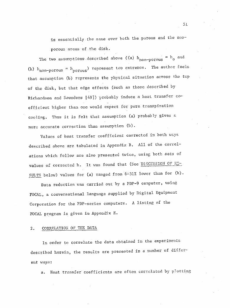
51

is essentially the same over both the porous and the non-

porous areas of.the disk.

The two assumptions described above ((a) h = ho

andnon-porous

(b) tenon-porous hporous) represent two extremes. The author feels

that assumption CO represents the physical situation across the top

of the disk, but that edge effects (such as those described by

Richardson and Saunders [49]) probably induce a heat transfer co-

efficient higher than one would expect for pure transpiration

cooling. Thus it is felt that assumption (a) probably gives a

more accurate correction than assumption (b).

Values of heat transfer coefficient corrected in both ways

described above are tabulated in Appendix B. All of the correl-

ations which follow are also presented twice, using both sets of

values of corrected h. It was found that (See'DISCUSSION OF RE-

SULTS below) values for (a) ranged from 6 317. lower than for (b).

Data reduction was carried out by a PDP-9 computer, using

FOCAL, a conversational language supplied by Digital Equipment

Corporation for the PDP-series computers. A listing of the

FOCAL program is given in Appendix E.

2. CORRELATION OF THE DATA

In order to correlate the data obtained in the experiments

described herein, the results are presented in a number of differ-

ent ways:

a.. Heat transfer.coefficients are often correlated by plotting

Nusselt number as a function of Reynolds number. Using

variables relevant to the rotating disk geometry (typical

length = R, typical velocity = wR), this might appear as

hRv s

wR2

k

Previous investigators of heat and mass transfer from

solid rotating disks [see 10, 33, 68] have presented their

experimental data in this way, as have others investigating

heat transfer theoretically [see 66].

Consequently, the grouping (hRik) for three different

injection rates has been calculated and plotted as a func-

52

[V-2]

2wR

tion of Re in Figures V-2a and b. Tabulated results

are found in Appendix B.

b. In laminar boundary layer heat transfer, results are

sometimes given as NuRe -2 vs. Pr (see Knudsen and Katz [32],

p. 482, for example). For the disk,

h(v/02k

NuRe 2= [V-3]

Instead of disk radius, Sparrow and Gregg have chosen (v/w)

as the normalizing length variable, referred to as d here.

Thus the right hand side in expression [V-3] may legitimately

be labeled a Nusselt number. Sparrow and Gregg's analysis

shows this Nusselt number to be independent of Reynolds number,

a result also found in laminar flow over a flat plate for

EuRe 2 Previously, Wagner [66] reached a similar conclusion

116

andcalculatedNu-k for a solid disk.

hRk

80

70

60

53

50 ec:cee"e

"S:ae-

40

Slope 4-

90% Conf. Interval.

30 0.41+0.51

20

10

9

8

15000 20000 30000 40000

Reynolds number wR2/v

50000

Figure V-2a. Effect of Reynolds Number and Injection On Heat Transfer

(h corrected, assuming hnon-porous = ho)

hRk

100

90

80

70

60

50

40

30

20

10

54

Slope +90% Conf. Intervals

0.95+0.24

O 0.35 lb/min ft2

0.73 lb/min ft2

A 1.04 lb/min ft 2

15000 20000 30000 40000 50000

Reynolds number wR2/v

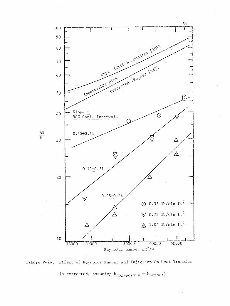
Figure V-2b. Effect of Reynolds Number and Injection-On Heat Transfer

(h corrected, assuming hnon_porous hporous)

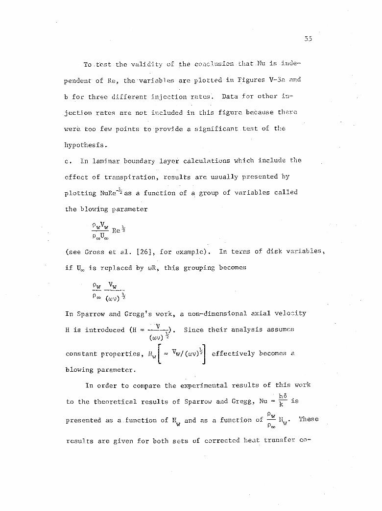
55

To test the validity of the conclusion that Nu is inde-

pendent of Re, the variables are plotted in Figures V-3a and

b for three different injection rates. Data for other in-

jection rates are not included in this figure because there

were too few points to provide a significant test of the

hypothesis.

c. In laminar boundary layer calculations which include the

effect of transpiration, results are usually presented by

plotting NuRe 2as a function of a group of variables called

the blowing parameter

pwVwRe

PC01j00

(see Gross et al. [26], for example). In terms of disk variables,

if U replaced by wR, this grouping becomes

pw Vw

P°°

In Sparrow and Gregg's work, a non-dimensional axial velocity

H is introduced (H = Vi). Since their analysis assumes

(wv)

[constant properties, Hw = Vw/(wv)1/2 effectively becomes a

blowing parameter.

In order to compare the experimental results of this work

116to the theoretical results of Sparrow and Gregg, Nu = is

Pwpresented as a function of H

wand as a function of ---H . These

n

results are given for both sets of corrected heat transfer co-

Prediced (aver {66]).Impermeable Disk

56

0 0.35 lb/min ft2

N7 0.73 lb/min ft2

A 1.04 lb/min ft2

15000 20000 30000 40000

Reynolds number coR2/y

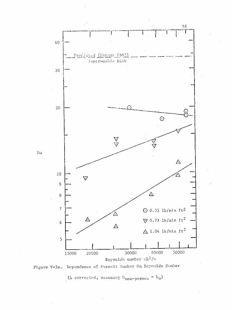
Figure V-3a. Dependence of Nusselt Number On Reynolds Number

50000

(h corrected, assuming h1 porous ho)

Nu

.57

80 17------1 F v--1--

70

60 0 0.35 lb/min ft2

N7 0.73 lb/min ft2

50 A 1.04 lb/min ft2

40

30

20

10

9

8

Predicted (Wagner ±661)

For Impermeable Disk

elamlewOHIO 0.

o

15000 20000 30000 40000 50000

Reynolds number wR2/v

Figure V-3b. Dependence of Nusselt Number On Reynolds Number

(h corrected, assuming h = hnon-porous porous )

58

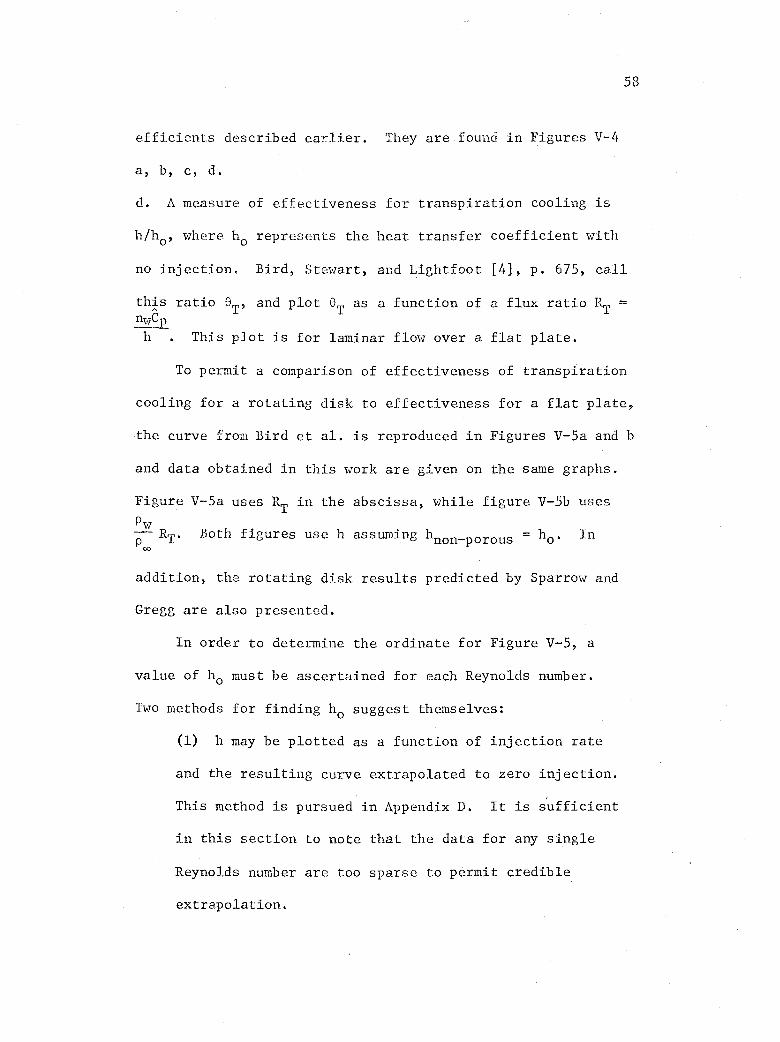
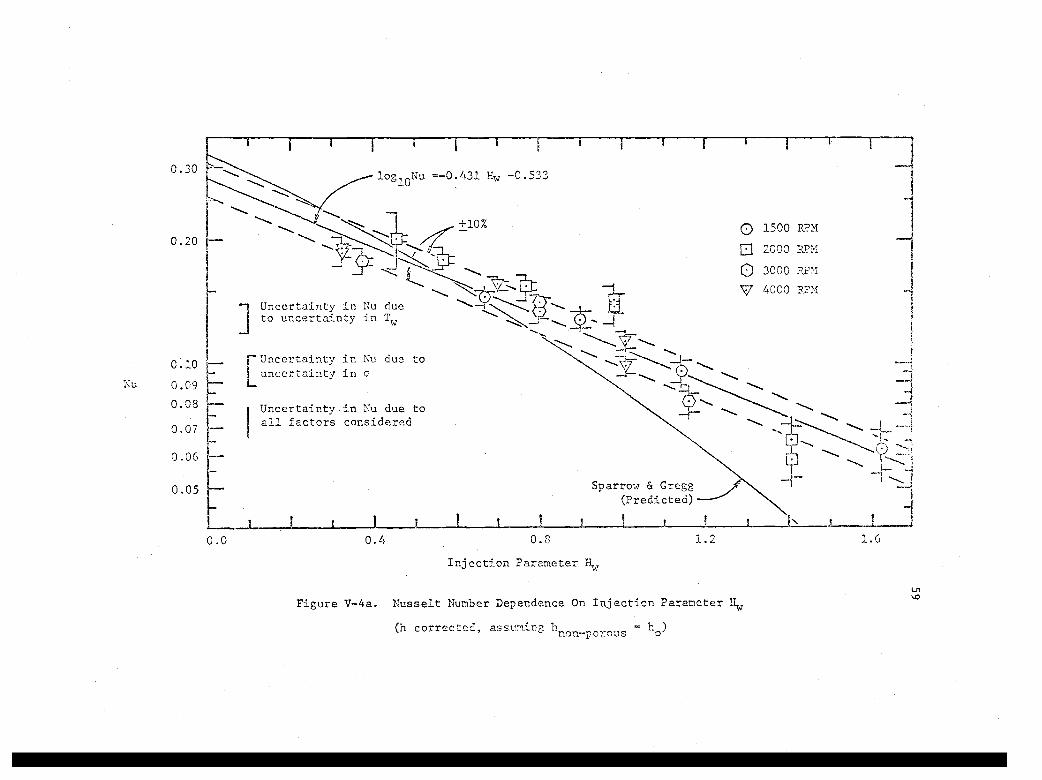
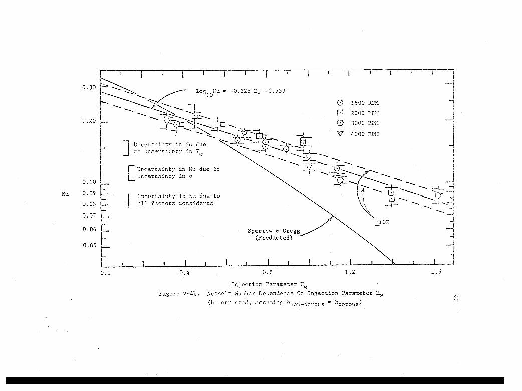
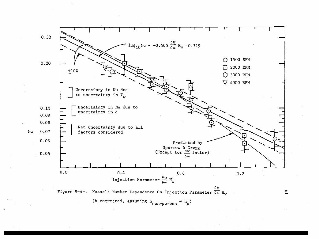
efficients described earlier. They are.found in Figures V-4

a, b, c, d.

d. A measure of effectiveness for transpiration cooling is

h/ho, where ho represents the heat transfer coefficient with

no injection. Bird, Stewart, and Lightfoot [4], p. 675, call

this ratio OT, and plot eT as a function of a flux ratio RT =nwCp

h . This plot is for laminar flow over a flat plate.

To permit a comparison of effectiveness of transpiration

cooling for a rotating disk to effectiveness for a flat plate,

the curve from Bird et al. is reproduced in Figures V-5a and b

and data obtained in this work are given on the same graphs.

Figure V-5a uses RT in the abscissa, while figure V-5b uses

PwRT. Both figures use h assuming tenon-porous = ho. In

P T' orous 0.

addition, the rotating disk results predicted by Sparrow and

Gregg are also presented.

In order to determine the ordinate for. Figure V-5, a

value of ho must be ascertained for each Reynolds number.

Two methods for finding ho suggest themselves:

(1) h may be plotted as a function of injection rate

and the resulting curve extrapolated to zero injection.

This method is pursued in Appendix D. It is sufficient

in this section to note that the data for any single

Reynolds number are too sparse to permit credible

extrapolation.

0Nu =-0.431 Hw -0.533

+10%

0.10

Nu 0.09

0.08

0.07

0.06

0.05

Uncertainty in Nu dueto uncertainty in Tw

rUncertainty in Nu due touncertainty in c

L.

Uncertainty in Nu due toall factors considered

0.0 0.4

1

0 1500 RPM

0 2000 RPM

0 3000 RPM

4000 PTM

0.8

Sparrow & Gregg(Predicted)

1.2 1.6

Injection Parameter Hw

Figure V-4a. Nusselt Number Dependence On Injection Parameter Hw

(h corrected, assuming h = h )non-porous

0.30

0.20

0.10

Nu 0.09

0.08

0.07

0.06

0.05

rz-f42-

Uncertainty in Nu dueto uncertainty in Tw

log Nu = -0.325 Hw -0.559

Uncertainty in Nu due touncertainty in o

1

0 1500 RPM

0 2000 ,R71.1

0 3000 RPM

V 4000 RPM

-7)

Uncertainty in Nu due to*

all factors considered

0.0 0.4

Sparrow & Gregg(Predicted)

0.8

1.

+10%

1.2

Injection Parameter Hw

Figure V-4b. Nusselt Number Dependence On Injection Parameter

(h corrected, aF's''ming tenon-porous hporous)

Hw

1.6

C,0

0.30

0.20

0.10

0.09

0.08

Nu 0.07

0.06

0.05

Pw1°g10Nu -0.505 -(3:-Hw -0.519

+10%

C) 1500 RPM

C] 2000 RPM

0 3000 RPM

V 4000 RPM OM'

1Uncertainty in Nu dueto uncertainty in Tw

[i

Uncertainty in Nu due touncertainty in a

Net uncertainty due to allfactors considered

MEN

Predicted bySparrow & Gregg

(Except for 2.17. factor)P.

0.0 0.4Pw

Injection Parameter 7)-; Hw

0.8

PwFigure V-4c. Nusselt Number Dependence On Injection Parameter pc., Hw

(h corrected, assuming h = h )non- porous

= h )

1.2

Nu

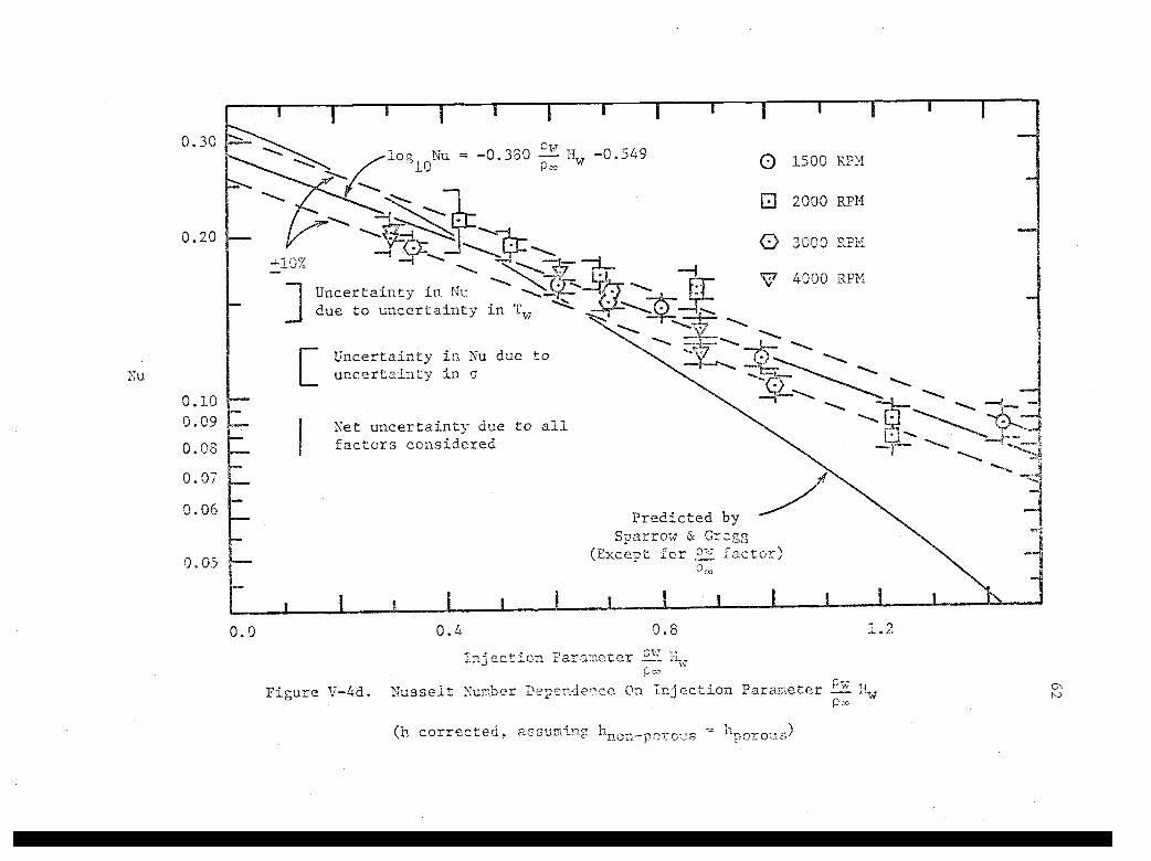
0.30logioNu = -0.330 -e-E H -0.549

w 0 1500 RPM

0 2000 RPM

0.20 C) 3000 RPM+10%

Uncertainty in NuN7 4000 RPM

due to uncertainty in T 1"--

_37

Uncertainty in Nu due touncertainty in

0.10

0.09 Net uncertainty due to all

0.03 factors considered

0.07

0.06 Predicted bySparrow & Gregg

07,

(Except for OW factor)P.0.05

0.0

Figure V-4d.

0.4 0.8 1.2

Injection Parameter al N.Pc

Nusselt Number Dependence On Injection Parameter EK Hw

(h corrected, assuming, hilon_oorous = hporoud

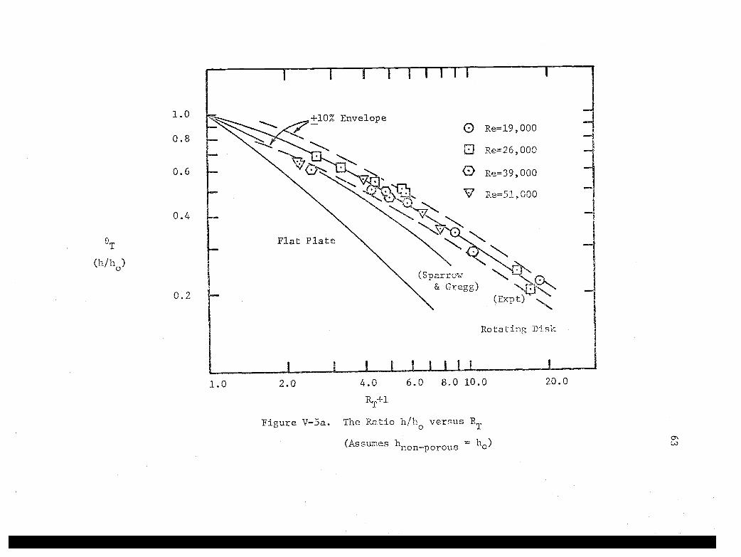
QT

(h/ho)

1.0

0.8

0.6

0.4

0.2

+10% Envelope

Flat Plate

C) Re=19,000

0 Re=26,000

CD Re=39,000

Re=51,000

(Sparrow& Gregg)

(Expt)

Rotating Disk

1.0 2.0 4.0

RT+1

6.0 8.0 10.0

Figure V-5a. The Ratio h/ho versus

(Assumes tenon-porous =

RT

20.0

eT

(h /ho)

1.0

0.8

0.6

0.4

0.2

Re=19,000

Re=26,000

C> Re=39,000

1.0 2.0 6.0 8.0 10.0

PwFigure V-5b. The Ratio h/h

oversus

(7;RT

(Assumes h = ho)non-porous

20.0

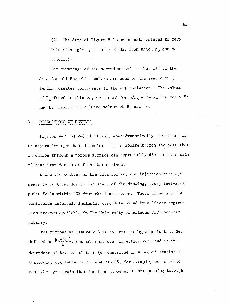
65

(2) The data of Figure V-4 can be extrapolated to zero

injection, giving a value of Nuo from which ho can be

calculated.

The advantage of the second method is that all of the

data for all Reynolds numbers are used on the same curve,

lending greater confidence to the extrapolation. The values

of ho found in this way were used for h/ho = OT in Figures V-5a

and b. Table D-1 includes values of 0T and RT.

3. DISCUSSIONS OF RESULTS

Figures V-2 and V-3 illustrate most dramatically the effect of

transpiration upon heat transfer. It is apparent from the data that

injection through a porous surface can appreciably diminish the rate

of heat transfer to or from that surface.

While the scatter of the data for any one injection rate ap-

pears to be great due to the scale of the drawing, every individual

point falls within 20% from the lines drawn. These lines and the

confidence intervals indicated were determined by a linear regres-

sion program available in The University of Arizona CDC Computer

Library.

The purpose of Figure V-3 is to test the hypothesis that Nu,

)defined as

11(y/w--- ---, depends only upon injection rate and is in-

dependent of Re. A "t" test (as described in standard statistics

textbooks, see Bowker and Lieberman [5] for example) was used to

test the hypothesis that the true slope of a line passing through

66

the data should be zero. For the three injection rates shown, the

results of the test at the 90% confidence level are as follows:

2lb/min ft test that slope = 0:

0.35 passes0.73 passes1.04 fails

A correct interpretation of the result is: if one desires a

90% assurance that he will avoid incorrectly rejecting the hypoth-

esis that the slope = 0, then that hypothesis must be accepted for

all but the highest injection rate. This result is used in Ap-

pendix D in a discussion of the detelmination of ho

.

In Figures V-4a-d, the data for all injection rates and all

rotational speeds are presented together. These figures show less

scatter than do the previous ones, demonstrating the advantage of

presenting a larger population when attempting to correlate ex-

perimental results.

Figures V-4a and b indicate the relationship between heat

transfer and injection rate, with rotational rate submerged in both

1 Vthe ordinate (11-

(v/w)1/2) and the abscissa ( w ). It is apparent

k (cov) 2

that the data can be reasonably well correlated with an equation

of the form

log10 Nu = B Hw + C [V-4]

where the particular values of the constants depend on the method

used to correct for the non-porous surface area. While nearly all

the data fall with a + 10% envelope, the envelope does-not coincide

67

with the theoretical prediction by Sparrow and Gregg for a sig-

nificant portion of the range of injection rate.

The form of the equation chosen [V-4] to correlate the data

has no special theoretical basis. However, it is more convenient

to plot the data on semi-log coordinates than log-log coordinates,

because of the need to extrapolate to zero injection. A logarithmic

ordinate was chosen so that equal vertical distances would represent

equal per cent error brackets.

It should be recalled that the analysis of Sparrow and Gregg

assumed constant fluid properties throughout the environment, regard-

less of temperature or concentration distributions within the flow.

This assumption is obviously invalid for foreign gas injection,

where the injectant might have drastically different properties

from the ambient fluid. That the assumption of constant properties

is inappropriate even for injection of air into air is indicated in

Figures V-4c and d.

Figures V-4c and d differ from V-4a and b only in the abscissa.

As indicated previously, transpiration heat transfer is commonly

correlated with an injection parameter

ox4Vw.

ReP.U.

which becomes

PwH

Pco w

when wR replaces U.. Naturally, if one could assume constant prop-

erties within the boUndary layer, the density ratio would be unity.

68

Since one cannot assume pw = p. even for.thetoderate temperature

excursions encountered.in this work, it would seem .more appropriate

to usePw-

Hw as the injection parameter, rather than simply Hw.

As seen in Figures V--4c and d, the data are again adequately

correlated by an equation of the form

1log10

Nu = + Ct [V-4

And again, as in Figures IVa and b, nearly all the points fall

within a +10% envelope. However, in the case of Figure V-4c, a

significant portion of the envelope includes the curve predicted

by Sparrow and Gregg. Restating the coincidence of the data and

Sparrow and Gregg's curve in another way, seventy per cent of the

points fall within 12% of the predicted curve.

One further way to illustrate the effect of transpiration

on heat transfer is given in Figures V-5a and b. In these figures,

h nwis presented as a function of a flux ratio h . Figure V-5a

shows that heat transfer coefficient can be decreased by as much

as 75-80% by injecting air through the surface. It also shows

that transpiration affects heat transfer from a rotating disk

less than from a flat plate in a uniform stream.

Note that the method of correlating the data illustrated

by Figure V-5b indicates a greater displacement from the predicted

result than does the correlation of Figure V-4c. This is probably

due to the dependence upon 110, an extrapolated value. It should be

1

noted that ho

from an extrapolation of Equation [V-4 ] is approximately

69

6% lower than ho from Sparrow and Gregg. This alone accounts for

a portion of the deviation of the experimental from the theoretical

result.

A final point of discussion of the data concerns natural con-

vection. For each run, the grouping Gr/Re2is tabulated in Appendix

B, Table B-2. As discussed in THEORY AND PREVIOUS WORK, this grouping

is a measure of the interference of natural convection with forced

convection heat transfer. According to the experimental results of

Richardson and Saunders 110] and the calculations of Fox [21], es-

2sentially no effect is to be expected for Gr/Re as low as 0.01.

Since the highest value for any run in the present experiments was

0.00115, no corrections have beeh made for natural convection.

70

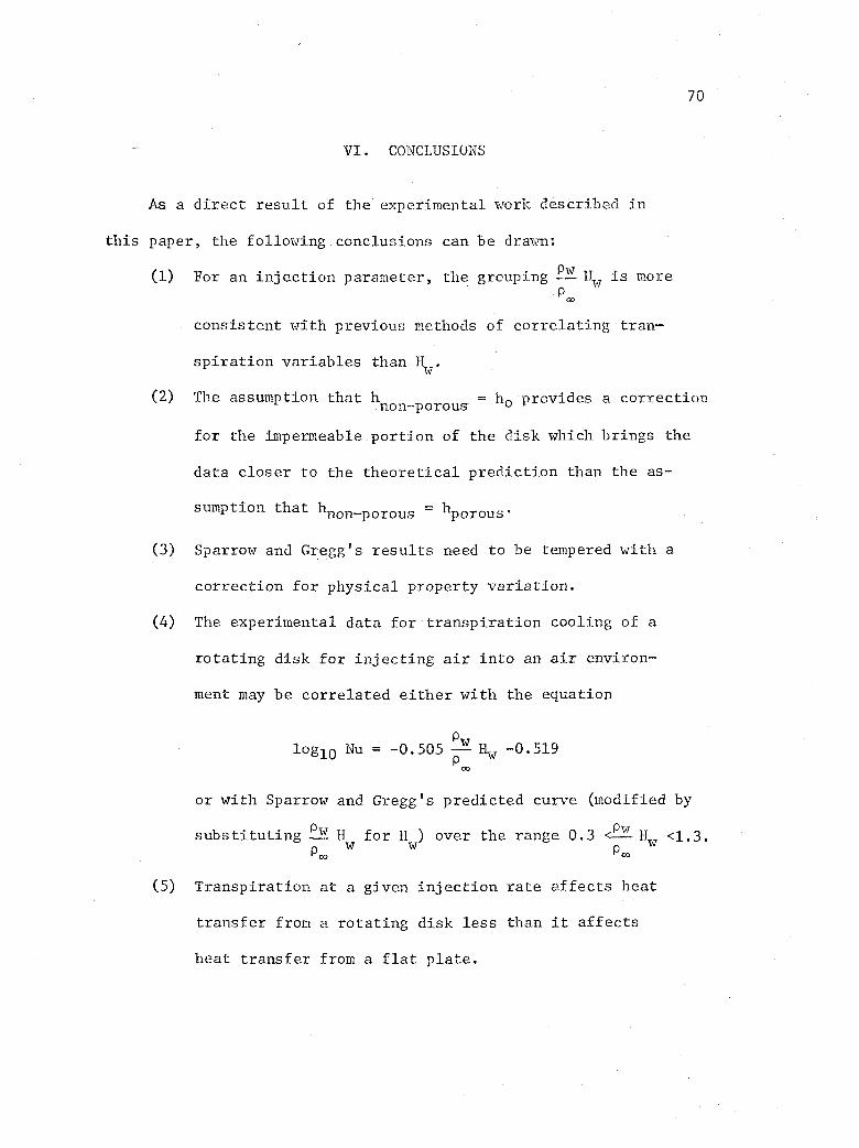
VI. CONCLUSIONS

As a direct result of the experimental work described in

this paper, the following conclusions can be drawn:

(1) For an injection parameter, the grouping Pw---Hw is more

consistent with previous methods of correlating tran-

spiration variables than H.

(2) The assumption that hnon-porous = h

0provides a correction

for the impermeable portion of the disk which brings the

data closer to the theoretical prediction than the as-

sumption that hnon_porous = hporous°

(3) Sparrow and Gregg's results need to be tempered with a

correction for physical property variation.

(4) The experimental data for transpiration cooling of a

rotating disk for injecting air into an air environ-

ment may be correlated either with the equation

per'log10 Nu = -0.505 ----p Hw -0.5190 0

or with Sparrow and Gregg's predicted curve (modified by

substituting i H for Hw) over the range 0.3 <-12E Hw <1.3.

Po, w Po,

(5) Transpiration at a given injection rate affects heat

transfer from a rotating disk less than it affects

heat transfer from a flat plate.

71

VII. SUGGESTIONS FOR.FURTHER.WORK

The next steps for further investigation of transpiration

cooling of a rotating disk should be as followst

1. Possible modification of the apparatus should be

investigated to permit a broadening of the range

of rotational rate and injection rate.

2. Transpiration cooling of a rotating disk with a

foreign gas should be attempted experimentally.

3. A theoretical investigation of transpiration cooling

of a rotating disk should be carried out which in-

cludes the effect of variable properties and possibly

the diffusion-thermo phenomenon (Soret effect). Cor-

relation of resultS might follow the form suggested

by the work of Mills and Wortman [42].

4. The work of Cooper [13] and Cham and Head [8] on the

turbulent boundary layer near a rotating disk should

be extended to include injection. The work of Kays [31]

and Cebeci [7] on the flat plate boundary layer could

serve as a model for the work. Both calculational and

experimental studies would be appropriate, though ex-

perimental difficulties may be insurmountable for the

high speeds necessary to attain turbulent flow.

72

BIBLIOGRAPHY

1. Andrews, R. D. and N. Riley. Unsteady heat transfer from a.rotating disk. Quarterly Journal of Mechanics and Applied

Mathematics 22:19-38. 1969.

2. Bayley, F. J. and J. M. Owen. The fluid dynamics of a shrouded

disk system with a radial outflow of coolant. Journal of Engi-

neering for Power 92:335-341. 1970.

3. Benton, Edward R. On the flow due to a rotating disk. Journal

of Fluid Mechanics- 24:781-800. 1966.

4. Bird, R. Byron, Warren E. Stewart, and Edwin N. Lightfoot. Trans-

port phenomena. New York, Wiley, 1960. 780 p.

5. Bowker, Albert H. and Gerald J. Lieberman. Engineering statistics.

Englewood Cliffs, Prentice-Hall, 1959. 585 p.

6. Boyd, K. E. and W. Rice. Laminar inward flow of an incompressiblefluid between rotating disks, with full peripheral admission.Journal of Applied Mechanics 35:229-237. 1968.

7. Cebcci, Tuncer. Behaviour of turbulent flow near a porous wallwith pressure gradient. AIAA Journal 8:2152-2156. 1970.

8. Chain, T. S. and M. R. Head. Turbulent boundary-layer flow ona rotating disk. Journal of Basic Engineering 93:199-204.

1969.

9. Chanaud, R. C. Measurements of mean flow velocity beyond arotating disk. Journal of Basic Engineering 93:199-204.

1971.

10. Cobb, E. C. and O. A. Saunders. Heat transfer from a rotatingdisk. Proceedings of the Royal Society, Ser. A, 236:343-351.1956.

11. Cochran, W. G. The flow due to a rotating disk. Proceedingsof the Cambridge Philosophical Society 30:365-375. 1934.

12. Conover, R. A. Laminar flow between a rotating disk and aparallel statIonary wall with and without radial inflow.Journal of Basic Engineering 90:325-332, 1968.

13. Cooper, Paul. Turbulent boundary layer on a rotating disk

calculated with an effective viscosity. AIAA Journal9:255-261. 1971.

14. Daily, J. W. and R. E. Nece. Chamber dimension effects on

induced flow and frictional resistance of enclosed ro-tating disks. Journal of Basic Engineering 82:217-232.

1960.

15. Davies, D. R.transfer intating disk.Mathematics

On the calculation of eddy viscosity and heata turbulent boundary layer near a rapidly ro-Quarterly Journal of Mechanics and Applied

12:211-221. 1959.

73

16. Davies, D. R. and C. B. Baxter. On the approximate calculationof heat transfer by laminar flow from a rotating heated diskat Prandtl numbers between 0.2 and 6. Quarterly Journal of

Mechanics and Applied Mathematics 14:223-228. 1961.

17. Davies, Owen L. (ed.) Statistical methods in research and

production. London, Oliver and Boyd,1961. 396 p.

18. Dewey, C. Forbes, Jr., and Joseph F. Gross. Exact similar

solutions of laminar boundary layer equations. Advances

in Heat Transfer 4:317-446. 1967.

19. Dorfman, L. A. Hydrodynamic resistance and the heat loss ofrotating solids. Edinburgh, Oliver and Boyd, 1963. 244 p.

20. Elzy, Eugene. Transpiration cooling of a cylinder in crossflow.Ph.D. Dissertation, Oregon. State University. June 1967. 315 p.

21. Fox, Jay. Effects of bouyancy on the laminar flow from anisothermal cone rotating in the quiet fluid. Journal ofHeat Transfer 86:560. 1964.

22. Fukusako, Shoichiro, Masaru Kiya, and Mikio Aire. Effects of

blowing or suction on the laminar boundary layer flow over arotating cone. Applied Scientific Research 23:269-280. 1970.

23. Goldstein, S. On the resistance of a disk immersed in a fluid.Proceedings of the Cambridge Philosophical Society 31:232-241.1935.

24. Goldstein, S. (ed.) Modern developments in fluid mechanics.London, Oxford University Press, 1938. 2 vols.

25. Gregory, N., J. T. Stuart and W. S. Walker. On the stabilityof three-dimensional boundary layers with application to flowdue to a rotating disk. Philosophical Transactions of theRoyal. Society of London, Ser. A, 248:155-199. 1956.

74

26. Gross, J. F., J. P. Hartnett, D. J. Masson, and C. Gazley, Jr.A review of binary boundary layer characteristics. Inter-national Journal of Heat and Mass Transfer 3:198-221. 1961.

27. Hering, R. G. and R. J. Grosh. Laminar combined convection froma rotating cone. Journal of Heat Transfer 85:29-34. 1963.

28. Homsy, G. M. and J. L. Hudson. Transient flow near a rotatingdisk. Applied Science Reviews 18:384-397. 1968.

29. Hudson, J. L. Nonisothermal flow between rotating disks.Chemical Engineering Science 23:1007-1020. 1968.

30. Jawa, M. S. A numerical study of axially symmetric flow betweentwo rotating infinite porous disks. Journal of Applied Me-chanics 38:683-687. 1971.

31. Kays, W. M. Heat transfer to the transpired turbulent boundarylayer. International Journal of Heat and Mass Transfer15:1023-1044. 1972.

32. Knudsen, James G. and Donald L. Katz. Fluid dymanics and heattransfer. New York, McGraw-Hill, 1958. 576 p.

33. Kreith, Frank, E. Doughman, and H. Kozlowski. Mass and heattransfer from an enclosed rotating disk with and withoutsource flow. Journal of Heat Transfer 85:153-163. 1963.

34. Kreith, Frank, J. H. Taylor and J. P. Chong. Heat and masstransfer from a rotating disk. Journal of Heat Transfer81:153-163. 1963.

35. Lehmkuhl, G. D. and J. L. Hudson. Flow and mass transfernear an enclosed rotating disk: Experiment. ChemicalEngineering Science 26:1601-1613. 1971.

36. Levich, Veniamin G. Physicochemical hydrodynamics. EnglewoodCliffs, Prentice-Hall, 1962. 700 p.

37. Lugt, H. J. and E. W. Schwiderski. Temperature distributions inrotating flows normal to a flat surface. Quarterly of AppliedMathematics 23:133-150. 1965.

38. Maroti, L. A., G. Deak and F. Kreith. Flow phenomena ofpartially enclosed rotating disks. Journal of Basic Engi-neering 82:539-552. 1960.

75

39. Matsch, L. and W. Rice. Flow at low Reynolds number withpartial admission between disks.. Journal of AppliedMechanics 34:768-770. 1967.

40. Matsch, L. and W. Rice. An asymptotic solution for laminar_flow of an incompressible fluid between rotating disks.Journal of Applied Mechanics 35:155-159. 1968.

41. Metzger, D. E. and J. W. Mitchell. Heat transfer from a

shrouded rotating disk with film cooling. Journal of

Heat Transfer 88:141-146. 1966.

42. Mills, A. F. and A. Wortman. Two-dimensional stagnationpoint flows of binary mixtures. International Journalof Heat and Mass Transfer 15:969-987. 1972.

43. Millsaps, Knox and Karl Pohlhausen. Heat transfer by laminarflow from a rotating plate. Journal of the AeronauticalSciences 19:120-126. 1952.

44. Mitchell, J. W. and D. E. Metzger. Heat transfer from ashrouded rotating disk to a single fluid stream. Journalof Heat Transfer 87:485-492. 1965.

45. Ostrach, Simon and Philip P. Thornton. Compressible laminarflow and heat transfer about a rotating isothermal disk.Washington, D. C., U. S. National Advisory Committee forAeronautics, 1958. 18 p. (Technical Note no. 4320.)

46. Oudart, Adalbert. Echanges thermiques pour le disque isothermeen rotation uniforme. Comptes Rendus 239:27-29. 1954.

47. Owen, J. M. The Reynolds analogy applied to flow between arotating and a stationary disc. International Journal ofHeat and Mass Transfer 14:451-460. 1971.

48. Owen, J. M. The effect of forced flow on heat transfer froma disc rotating near a stator. International Journal of Heatand Mass Transfer 14:1135-1147. 1971.

49. Richardson, P. D. and O. A. Saunders. Studies of flow and heat

transfer associated with a rotating disc. Journal of MechanicalEngineering Science 5:336-342. 1963.

50. Rogers, M. H. and G. N. Lance. The. rotationally symmetric flow

of a viscous fluid in the presence of an infinite rotating disk.Journal of Fluid.Mechanics 7:617-631. 1960..

76

51. Schlichting, H. .Boundary layer theory. 4th . New:York,

McGraw-Hill, 1960, 647 p.

52. Schultz-Crunow; F. Die Reibungwideratand rotierender Scheibenin Gehausen. Zeitschrift fur angewandte MatheMatik andMechanik 15:191-204.- 1935.

53. Schwiderski, E. W. and H. J. Lugt. Rotating flows of von Karman

and Bodewadt. Physics of Fluids 7:867-875. 1964.

54. Smith, Newell H. Exploratory investigations of laminar boundarylayer oscillations on a rotating disk. Washington, D. C., U. S.National Advisory COmmittee for Aeronautics, 1947. 15 p.

(Technical Note no. 1227.)

55. Society of Automotive Engineers. Recommended ice bath forreference junctions. Aerospace Reeommended Practice 691,August 1, 1964. 3 unnumb. leaves.

56. Soo, S. L. Laminar flow over an enclosed rotating disk.Transections of the American Society of Mechanical Engi-neers 80:287-296. 1958.

57. Sparrow, E. M. and J. L. Gregg. Mass transfer, flow, and heattransfer about a rotating disk. Journal of Heat Transfer82:294-302. 1960.

58. Sparrow, E. M., C. J. Scott, R. J. Forstrom and W. A. Ebert.Experiments on the diffusion-thermo effect in a binary bound-ary layer with injection of various gases. Journal of HeatTransfer 87:321-328. 1965.

59. Stuart, J. T. On the effects of uniform suction of the flow dueto a rotating disk. Quarterly Journal of Mechanics and AppliedMathematics 7:446-457. 1954.

60. Tewfik, O. E. and Ji-Wu Yang. Emissivity measurements of porousmaterials. Journal of Heat Transfer C85:79-80. 1963.

61. Theodorsen, T. and A. Regier. Experiments on drag of revolvingdisks, cylinders, and streamline rods at high speeds.Washington, D. C., U. S. National Advisory Committee forAeronautics, 1944. (Technical Report no. 793, from ThirtiethAnnual Report, p. 367-384.)

62. Tien, C. L. Heat transfer by the induced flow about a rotatingcone of non-uniform surface temperature. International Journalof Heat and Mass Transfer 8:411-418. 1965.

77

63. Tien, C. L. and J. Tsuji. Heat transfer by laminar forcedflow against a non-isothermal rotating disk. International

Journal of Heat and Mass Transfer 7:247-252. 1964.

64. Tomlan, P. F. and J. L. Hudson. Flow near an enclosed rotatingdisk: analysis. Chemical Engineering Science 26:1591-1600.

1971.

65. von Kaman, T. Uber laminare und turbulente Reibung. Zeitschrift

fur angewandte Mathematic und Mechanik 1:233-252. 1921.

(Translated in U. S. National Advisory Committee forAeronautics Technical Memorandum no. 1092. 1946. 39 p.)

66. Wagner, Carl. Heat transfer from a rotating disk to ambientair. Journal of Applied Physics 19:837-839. 1948.

67. Wortman, A., A. F. Mills and G. Soo Hoo. The effect of masstransfer on recovery factors in laminar boundary layer flows.International Journal of Heat and Mass Transfer 15:443-456.

1972.

68. Young, R. L. Heat transfer from a rotating plate. Transactionsof the American Society of Mechanical Engineers 78:1163-1168.1956.

APPENDICES

78

APPENDIX A

EXPERIMENTAL DATA

Table A-1. Experimental Data.

Run No.(Date)

No. RPM w

1sec--

wlb

nlb

Tc

oFTw°F

T,

°F

Tw.

°T.

huncorr

Btu

Re

min min ft2 hr ft2 °F

9017101 1 1520 159 0.0365 0.440 167.6 143.2 92.3 85.4 2.59 20,300

9017102 2 1500 157 0.0481 0.580 185.4 162.5 93.8 87.4 2.33 19,500

9017103 3 1500 157 0.0600 0.723 207.3 187.5 100.7 90.8 1.89 18,600

9027101 4 1520 159 0.0867 1.045 189.7 179.6 100.2 87.7 1.43 19,000

8317101 5 2150 225 0.0300 0.362 153.5 122.5 86.1 82.5 4.02 29,900

8317102 6 2050 214 0.0363 0.438 167.7 137.6 90.0 84.5 3.55 27,600

8317103 7 2040 214 0.0480 0.579 185.9 158.4 94.5 86.7 3.13 26,500

8317141 8 2040 214 0.0609 0.734 194.6 171.3 99.5 88.4 2.96 25,900

8317142 9 2040 214 0.0608 0.733 194.9 171.3 96.8 88.4 2.88 26,000

9027121 10 2050 215 0.0866 1.044 193.1 181.1 98.2 88.3 1.70 25,600

9027122 11 2050 215 0.0866 1.044 192.9 181.5 98.7 88.3 1.58 25,600

9267101 12 3010 315 0.0289 0.348 168.7 129.4 87.3 82.1 4.26 41,400

9037111 13 3020 316 0.0603 0.727 198.5 170.6 97.4 88.1 3.54 38,400

9037112 14 3030 317 0.0604 0.728 199.5 172.2 98.3 88.5 3.40 38,400

9027103 15 3010 315 0.0865 1.043 199.1 183.2 98.8 88.5 2.34 37,500

9267121 16 4000 419 0.0289 0.348 183.7 133.8 88.4 85.4 5.11 54,600

9267122 17 4000 419 0.0289 0.348 183.7 133.4 88.4 85.4 5.21 54,600

9037103 18 4000 418 0.0603 0.727 212.3 176.3 99.3 88.9 4.42 50,200

9027141 19 4000 419 0.0865 1.043 205,1 184.6 98.9 88.3 3.11 49,700

9027142 20 4000 419 0.0864 1.041 207.9 185.3 99.1 88.1 3.46 49,600

80

APPENDIX B

CALCULATED RESULTS

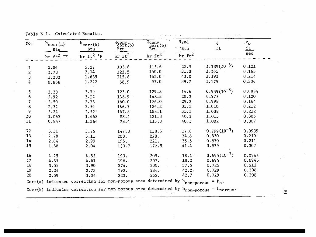
Table B-1. Calculated Results.

No. h h gconvqconv grad vwcorr(a) corr(b) corr(b) Tr(b)Btu Btu Btu BtuBtu ft ft

hr ft2 °F hr ft2 °F hr ft2 hr ft2 hr ft2sec

1 2.042 1.783 1.3334 0.868

5 3.386 2.927 2.508 2.329 2.24

10 1.06311 0.947

12 3.5113 2.7814 2.6415 1.58

16 4.2517 4.3518 3.5519 2.2420 2.59

Corr(a) indicates correction for non-porous area determined by hnon-porous = ho.

Corr(b) indicates correction for non-porous area determined by hnon_porous = hporous

2.272.041.6351.222

3.553.122.752.59

2.521.4681.364

3.763.112.99

2.04

4.534.613.902.733.04

103.8122.5115.868.9

123.0138.9160.0166.7167.388.478.4

147.8203.

195.133.7

193.196.274.

192.223.

115.6140.0142.097.0

129.2148.8176.0186.2188.1121.8113.0

158.6228.

221.172.5

205.

207.

300.234.

262.

22.531.043.0

39.7

14.620.329.235.135.140.340.5

17.634.835.541.4

18.418.237.542.242.7

1.1r5(10-3)

1.1931.179

0.939(10-3)0.9770.9981.0101.0081.0151.002

0.799(10-3)0.8300.8300.839

0.695(10-3)0.6950.7250.7290.729

0.1210.1650.2140.306

0.09640.1200.1640.2120.2120.3060.307

0.09390.2100.2110.307

0.09460.09460.2120.3080.308

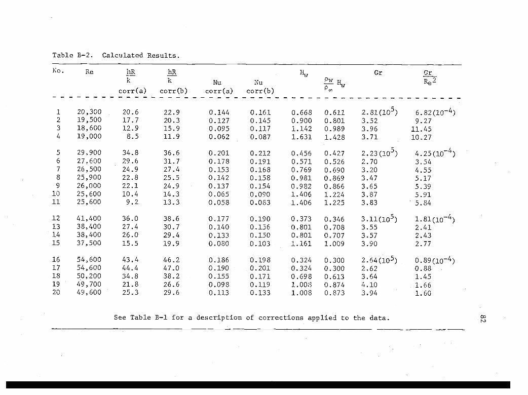
Table B-2. Calculated Results.

No. Re hRk

corr(a)

hRk

corr(b)Nu

corr(a)Nu

corr(b)

HwPw 77

r3W

Gr GrRe2

Po,

1 20,300 20.6 22.9 0.144 0.161 0.668 0.611 2.81(105 ) 6.82(10-4)2 19,500 17.7 20.3 0.127 0.145 0.900 0.801 3.52 9.273 18,600 12.9 15.9 0.095 0.117 1.142 0.989 3.96 11.454 19,000 8.5 11.9 0.062 0.087 1.631 1.428 3.71 10.27

5 29,900 34.8 36.6 0.201 0.212 0.456 0.427 2.23(105 ) 4.25(10-4 )

6 27,600 29.6 31.7 0.178 0.191 0.571 0.526 2.70 3-547 26,500 24.9 27.4 0.153 0.168 0.769 0.690 3.20 4.558 25,900 22.8 25.5 0.142 0.158 0.981 0.869 3.47 5.179 26,000 22.1 24.9 0.137 0.154 0.982 0.866 3.65 5.39

10 25,600 10.4 14.3 0.065 0.090 1.406 1.224 3.87 5.9111 25,600 9.2 13.3 0.058 0.083 1.406 1.225 3.83 5.84

12 41,400 36.0 38.6 0.177 0.190 0.373 0.346 3.11(105) 1.81(10-4)13 38,400 27.4 30.7 0.140 0.156 0.801 0.708 3.55 2.4114 38,400 26.0 29.4 0.133 0.150 0.801 0.707 3.57 2.4315 37,500 15.5 19.9 0.080 0.103 1.161 1.009 3.90 2.77

16 54,600 43.4 46.2 0.186 0.198 0.324 0.300 2.64(105) 0.89(10-4)17 54,600 44.4 47.0 0.190 0.201 0.324 0.300 2.62 0.8818 50,200 34.8 38.2 0.155 0.171 0.698 0.613 3.64 1.4519 49,700 21.8 26.6 0.098 0.119 1.008 0.874 4.10 1.6620 49,600 25.3 29.6 0.113 0.133 1.008 0.873 3.94 1.60

See Table B-1 for a description of corrections applied to the data.

83

APPENDIX C

SOURCES OF ERROR

84

.SOURCES OF ERROR .

Sources of error in the heat transfer coefficients presented

in this work can be classified as follows:

1. Experimental error

2. Uncertainty in the value of emissivity

3. Uncertainty in the method of correcting

for the impermeable area of the disk

Each of these categories is discussed in turn. A final category,

4. Sum of uncertainties,

indicates how the errors discussed in the previous sections are com-

bined statistically to give an estimate of the total uncertainty in h.

1. EXPERIMENTAL ERROR

Uncertainties in h due to experimental error arise in the

measurement of temperatures and in the measurement of flow rate.

a. Errors in Temperature Measurement

The effect on calculated values of h due to errors in temp-

erature measurement was determined in the following way: An estimate

of the uncertainty of each temperature measurement was made (as de-

scribed below), resulting in a range of values having a high proba-

bility of including the true value. Then the measured value of the

temperature, and also the estimated extreme values of the range of

the temperature, were used sequentially as inputs for the data re-

duction program described in Appendix E.

85

By carrying out this procedure for each experimental run, the

sensitivity of h to error.in Tw, T and T . was determined. Re-

sults are presented numerically in Table C-1 and graphically in

Figures V-4a, b, c, d by horizontal bracketS facing left (see

legend).

The values given in Table C-1 are for AT (estimated uncertainty

in T), Ah (resulting from AT), and DT (sensitivity of h to uncer-

tainties in T, calculated as the quotient Ah/AT).

Since errors are combined (see Section 4 below) according to

the formula

= AhAh2total

the values in Table C-1 indicate that the error in h due to uncer-

tainty in To, is always less than 12% of that due to certainty in Tw.

During the experimental runs, there was uncertainty in the true

value of T due to uncertainty in the calibration curve and to

fluctuations in the millivolt reading of the infrared radiometer.

Calibration curve uncertainty was determined by adding the errors

of (a) long term drift (estimated as one-half the drift observed

over the succeeding 24 hours), and (b) other feasible curves drawn

through the same set of calibration points. Error due to electronic

noise was assumed to be less than one-half the difference between the

highest value observed during any particular measurement and the av-

erage value. The estimate of the uncertainty in Tw given in Table C-1

was obtained by combining the above possible errors.

Table C-1. Estimated Experimental Uncertainty.

No. h**

*

AT.

*

Abroo ah

no,*

ATw AhTw Aha ELh100 EAhDTw

1 2.04 0.5 0.03 0.05 0.5 0.09 0.16 0.08 0.12 62 1.78 0.5 0.015 0.03 0.5 0.06 0.14 0.09 0.11 63 1.333 1.2 0.024 0.02 0.5 0.07 0.14 0.09 0.12 94 0.868 1.2 0.024 0.02 0.5 0.11 0.20 0.09 0.14 175 3.38 0.3 0.03 0.10 2.0 0.53 0.25 0.09 0.54 166 2.92 0.7 0.05 0.07 1.0 0.22 0.2 0.08 0.24 87 2.50 0.6 0.03 0.05 1.0 0.18 0.17 0.09 0.20 88 2.32 0.6 0.02 0.03 1.0 0.20 0.18 0.09 0.22 109 2.24 0.6 0.02 0.03 1.0 0.20 0.18 0.09 0.22 1010 1.063 1.0 0.02 0.02 0.5 0.10 0.18 0.09 0.14 1411 0.947 1.0 0.02 0.02 0.5 0.10 0.18 0.09 0.14 14

12 3.51 0.3 0.03 0.10 1.0 0.23 0.21 0.08 0.25 713 2.78 0.8 0.04 0.05 0.7 0.14 0.17 0.09 0.17 614 2.64 0.8 0.04 0.05 0.7 0.14 0.17 0.09 0.17 615 1.58 0.8 0.024 0.03 0.5 0.11 0.20 0.09 0.14 916 4.25 0.3 0.03 0.10 1.5 0.34 0.22 0.08 0.35 817 4.35 0.3 0.03 0.10 1.5 0.34 0.22 0.08 0.35 818 3.55 0.7 0.035 0.05 0.6 0.12 0.18 0.09 0.15 419 2.24 1.0 0.03 0.03 0.5 0.11 0.20 0.09 0.15 620 2.59 1.0 0.03 0.03 0.5 0.11 0.20 0.09 0.15 6* Units of h and Lh are Btu/hr ft2 °F. Units of AT are °F, and those for Thin areBtu/hr ft2 °F2.

** Corrected assuming hnon_ = hoporouscocr,

87

Uncertainty in .the value of T. was due to. fluctuations of the

reading during a particular.. run. While the. thermocouples were not

inherently noisy transducers, nonetheless there were fluctuations

of + 20 to 70 microvolts. (+ 0.6 to 2.4°F) due to.convection

currents within the environment. The estimate of uncertainty in

T. given in Table C-1 is one-half the fluctuations .described above.

It is assumed that errors due to calibration'of the thermocouples

were negligible compared to the uncertainties reported in Table C-1.

Uncertainties in h due to possibleeriors in T were consideredwc,

negligible. Tw. measurements were quite stable, showing only very

small (0-6 microvolts) fluctuations for every run.

b. Errors In Flow Measurement

As discussed under EXPERIMENTAL EQUIPMENT, calibration of the

orifice meter was accurate to +1/2%. An error of this magnitude

would not be discernible on Figure V-4. As shown in Appendix F,

possible leakage in the system is also negligible.

2. UNCERTAINTIES IN THE VALUE OF EMISSIVITY

As discussed under EXPERIMENTAL EQUIPMENT, the emissivity of

the porous surface was taken as 0.3, the value obtained by a pre-

vious investigator [20] using the same type of material from the

same manufacturer. It is recognized, however, that some slight

difference in fabrication may have caused a slightly different

surface condition of the stainless steel wire mesh. A range of

88

0.25-0.35 is assumed to .be'broad enough to include.thetrue value

of emissivity.

To determine the error in heat transfer coefficient possible

because of the uncertainty in the value of emissivity described

above, h was calculated using three values of emissivity: 0.25,

0.30, and 0.35. The range in h is given numerically in Table C-1

as Ahc./ and shown graphically in Figures V-4a, b, c, d by horizontal

brackets facing right (see legend).

3. UNCU: x IN CORRECTION FOR IMPERMEABLE AREA

The two methods of correcting for the outer, non-porous area

of the rotating disk were discussed at some length under RESULTS.

Certainly the assumption that h = h provides anporous

indisputable lower limit for the correction. The other assumption

used to calculate a second estimate of the correction, viz.,

tenon- porous ho (h for no injection) could possibly be argued

inadequate as an upper limit. For example, 110 for a rotating cyl-

inder might give a better upper limit. Or some arbitrary multiple

of hofor a rotating disk might be used, or ho

for turbulent flow

over a disk might be used.

The author feels, however, that the value used is adequate

and is readily calculated from the data at hand. Quantitative

estimates for the other corrections suggested above would be

difficult to determine And.more difficult to justify. Therefore,

89

it is assumed that the two,corrections calculated.for.the.non-

porous area of the disk provide adequate upper and lower limits.

4. SUM OF UNCERTAINTIES

The individual uncertainties described in the sections 1 and

2 above contribute to the total uncertainty in the heat transfer

coefficient. To determine the total uncertainty, the individual

uncertainties must be combined in a statistically appropriate way.

According to Davies [17], if y is a function of several vari-

ables xl, x2 . . ., then the variance of y (i.e., the square of the

standard deviation) is given by:

s2 .ifty 12 s2 4:8

x1 3x2 x

2

[C-1]

This equation assumes no interaction among the variances of x1, x2...

(covariance = 0).

To translate this formula into the present problem, several

substitutions and assumptions will be made. First, h is substi-

tuted for y, Tw for xl, T. for x2 and a for x3. Second, recognizing

that standard deviation or standard error describes the tendency

of a measurement to be distributed about the mean, the estimated

error of a given variable is substituted for a multiple of its

standard deviation, i.e.

ATest = N sT

Finally, it is assumed that the errors estimated in each of the

90

previous sections enclosed limits at equal levelS of significance,

i.e. if

and if

Nest N Rest 1 -T

Aoest = N2

so

then it is assumed that N1

= N 2 . Making the above substitutions,

equation [C-1] becomes

Ah22 2 2

= DI AT2 + Ml- AT.0 + ah 2 Ac2(

i",,,,, w aT,, ao

[C-2]

If we replace AT with AhT,aT as described in section 1 above, and

ah

ac5Ac with Ah0' then

Ah2 = Ah2 + Ah T + Ah2Tw a

[ C-3 ]

Equation [C-3] embodies the method used to combine individual

errors in order to estimate the total uncertainty in heat transfer

coefficient presented in this work. While the individual uncer-

tainties are indicated in Figures V-4a, b, c, d with brackets

facing right or left, the total uncertainty is indicated by a

vertical line. It is also presented in Table C-1, both in terms

of Ahtotal and as a per cent of h.

It is recognized that the total uncertainty in h may be larger

than the values tabulated due to factors not quantitatively accounted

for. For example, if the heat transfer coefficient for the non-

porous area of the disk is different from that calculated, the actual

91

value of h could fall beyond the limits indicated in Figuresporous

V-4a, b, c, d. Nonetheless, the author submits these intervals,

with a high degree of confidence, as estimates of a range of values

into which the true value of h falls.

92

APPENDIX D

EXTRAPOLATING h TO FIND ho

93

EXTRAPOLATING h TO FIND 110

Many of the calculations described in. EXPERIMENTAL RESULTS

required values for 110, the heat transfer coefficient for zero

injection. Since the apparatus described herein did not permit

the direct determination of heat transfer with zero injection,

it was necessary to find 110 by extrapolation.

Extrapolation of experimental data is, of course, subject

to error. Experimental error causes some degree of uncertainty

within the range of the variables studies. Futhermore, when one

extrapolates outside of the range of experimentation, the uncer-

tainty may become magnified. For this reason, the method used to

extrapolate should be chosen carefully so as to minimize the effect

of experimental uncertainty on values obtained in this way.

Two methods of extrapolation were attempted for finding bp.

The first isolated the data for a given rotational rate, plotted

h as a function of injection rate, then extrapolated a line through

those points to zero injection. Data for this method are compiled

in Table D-1, corrected for minor deviations from the nominal

rotational speed, and plotted in Figure D-1. It is apparent from

the figure that this method is unsatisfactory because, for any one

rate of rotation, there are so few data points that the uncertainty

causes a very high uncertainty in the extrapolated value at zero

injection.

The second method of extrapolation overcomes many of the ob-

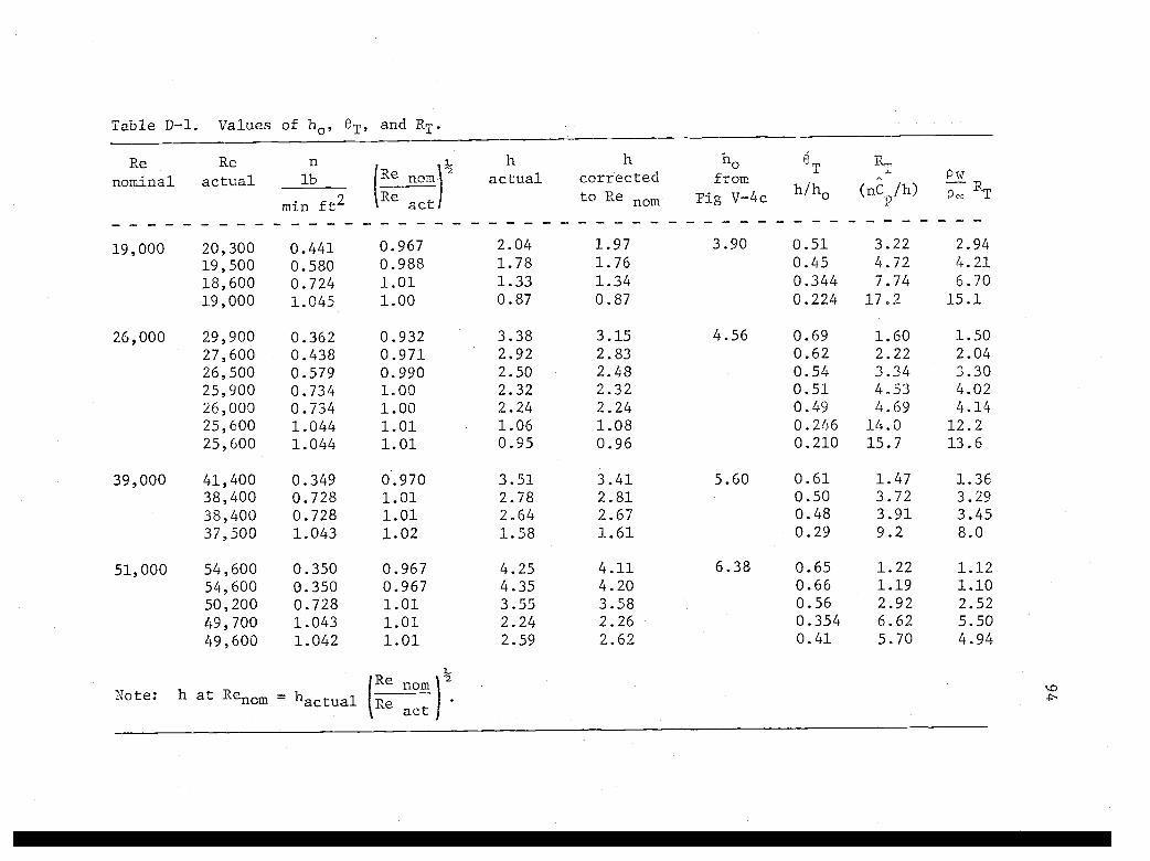
Table D-1. Values of 110, eT, and RT.

Renominal

Re n

actual lb (Re nomh

actual

h

correctedto Re

110

from

Fig V-4c

T

h/ho

R.

(nC /h)Pwpeo RT

min ft2Re act

19,000 20,300 0.441 0.967 2.04 1.97 3.90 0.51 3.22 2.94

19,500 0.580 0.988 1.78 1.76 0.45 4.72 4.21

18,600 0.724 1.01 1.33 1.34 0.344 7.74 6.70

19,000 1.045 1.00 0.87 0.87 0.224 17.2 15.1

26,000 29,900 0.362 0.932 3.38 3.15 4.56 0.69 1.60 1.50

27,600 0.438 0.971 2.92 2.83 0.62 2.22 2.04

26,500 0.579 0.990 2.50 2.48 0.54 3.34 3.3025,900 0.734 1.00 2.32 2.32 0.51 4.53 4.02

26,000 0.734 1.00 2.24 2.24 0.49 4.69 4.1425,600 1.044 1.01 1.06 1.08 0.246 14.0 12.225,600 1.044 1.01 0.95 0.96 0.210 15.7 13.6

39,000 41,400 0.349 0.970 3.51 3.41 5.60 0.61 1.47 1.3638,400 0.728 1.01 2.78 2.81 0.50 3.72 3.29

38,400 0.728 1.01 2.64 2.67 0.48 3.91 3.45

37,500 1.043 1.02 1.58 1.61 0.29 9.2 8.0

51,000 54,600 0.350 0.967 4.25 4.11 6.38 0.65 1.22 1.12

54,600 0.350 0.967 4.35 4.20 0.66 1.19 1.10

50,200 0.728 1.01 3.55 3.58 0.56 2.92 2.52

49,700 1.043 1.01 2.24 2.26 0.354 6.62 5.50

49,600 1.042 1.01 2.59 2.62 0.41 5.70 4.94

Re nomNote: h at Renom = -actual Re act

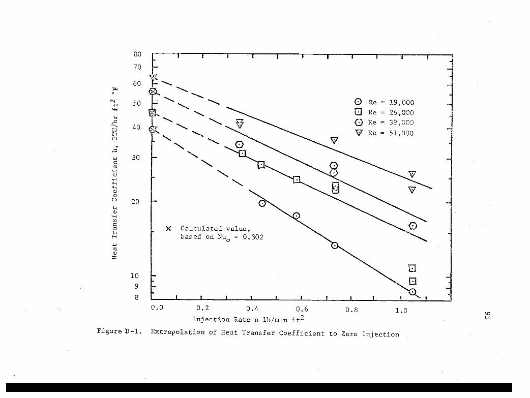
80

70

60

50

40

30

20

10

9

8

0

X Calculated value,based on Nu

o = 0.302

V

0 Re = 19,000

0 Re = 26,000

O Re = 39,000

N7 Re = 51,000

9

0.0 0.2 0.4 0.6

Injection Rate n lb /min ft2

Figure D-1. Extrapolation of Heat Transfer Coefficient to Zero Injection

0.8 1.0

96

jections to the first. ThiS method used all of the data for all

rotational rates and all injection rates, as plotted on Figure

V-4c. Since there are many more data points, one has greater

confidence in the inferred relationship, and thus in the ex-

trapolated value of Nuo and ho.

Using standard statistical techniques (see[5] for example),

a confidence interval was determined for the intercept of the line

inferred by the linear regression technique. At the 98% confidence

level,

Or

log10

Nuo= -0.51962 + 0.0247

Nuo = 0.302 + 0.017

Thus, with 98% confidence, Nuo and 110 are estimated within a 6%

interval.

w)liThe conversion of Nuo to 110 is obvious, since Nu -

h(v/

Interestingly, the ratio k/v2 is very nearly independent of tem-

perature (the variation from 90°F to 150°F is less than 1/2%) for

air, so one can choose either environment temperature or film tem-

perature to evaluate fluid properties when calculating 110 from Nuo.

The data reduction program used film temperature (Taira =0.5

(TW

+ Tom)).

It should be noted that the determination of Nuois actually

an iterative procedure. Each data point on Figure V-4c required

a value for 110 in calculating the correction for the non-porous

97

portion of the rotating disk. Because the non - porous area is only

about 11% of the total area, however, the extrapolated value of Nuo

was rather insensitive to the value used in the correction. For

example, a 10% change in the value of Nuo used for the correction

caused a change of only 1.2% in the extrapolated value of Nuo.

The last four columns of Table D-1 present the values of ho

for each nominal Reynolds number and 0T for each run (corrected

to nominal Re), and RT andPw

T The significance of these data

is discussed in EXPERIMENTAL RESULTS. They are plotted in Figures

V-5a and b.

98

APPENDIX E

DATA REDUCTION PROGRAM

99

DATA REDUCTION PROGRAM

The following program was used to convert the raw data, re-

corded in millivolts, centimeters of manometer fluid, millimeters

of mercury, etc., to heat transfer coefficients, Reynolds numbers,

Nusselt numbers, etc. It is written in FOCAL, a conversational

language provided by Digital Equipment Corporation for users of

their PDP-series computers. The computer used was a PDP-9 in the

College of Mines Computing Laboratory at The University of Arizona.

-/tc,..,T.

(.;7=1-'1;/ .1`:-.:),/=L4-t117:r=.;TH3,-;f.:;172:N:VI;;4.t

I".;

4=ti).174I\,71)=4"CI=ii =Alt-11.Cllii 1CrifI.4I.=4. 31

L

Id=t

(;-',1.;',TnLCFT.f-11T.v)

,3T(1(1 T 1)'..11j11-11)CCC

-I1'I=I° L.)/!-!,I

(1)4**7-7:lIL-F,;1,1EC

( 4 'N'Tf.`11ur '.'I,)=f.t; =iCCC !1..1))4' . !=/ :)1ftttI ==1:1{,1Ij.-:-;I

1(-;I.1.)=4r-T fClN,r1= 1L I.i

I / ( 9(+)=IL717CtIl ;-fI11717f,L)=1Vi

'\1-ICII1.

(111

-I 4: r,Y)\-.;;`,1N/, A1

i7tvTC17Jc-:-/)*1-14717,71;iT

r17'L:\j1CC) C, 174 g.11',IIIC. I. (1 IN' Iti I it.I.C 1I I

- 717 f) 11 1".)I II

(:)

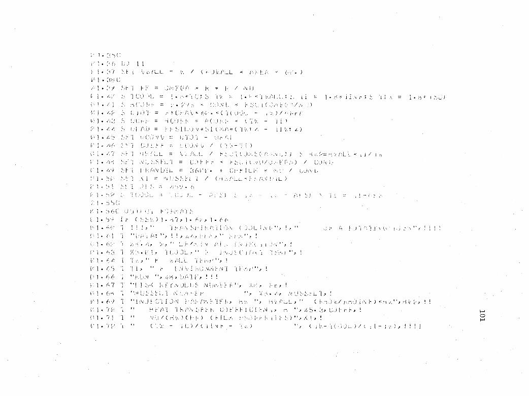
V 1

1 . L.) 1 1

V. 1 ;- 7 .-.;

.

I ,.,. ',,,, I'LL = .,, / ( ....) ,iLL... H: -!= (.--,v. )

V I 3 -.', (..;

I :',:-) ..`.',i- 'I I- i; = Jiv 1; C., .i.T.: .* !,: -,,K I, / N 0( I ii,/' ..:, 'I (..:0 ..)1..._ = I .:.-",

.,., 'i C; S 'i. ,,,, = I '...; `i .(4... L. ; :-...: '1 i =1 --..

: i i .\.; 1- ; :.--:. 1 I ...^,.= 1

v, 1 L I ::-, H (.:J ;-... is. z--..,,...: .-,,,.?';,-., Jr.: r,,...) A; I; ,,,- )-. ,:::; (.,.,., i ( .J,v) 1-.7 ;::(..'-, ,.....D

VI I /,`:-- .5 L j ti 1 - = ',,,, (....":1---. \)* t':,,v i, ( I L.),..)1..... -'; %,,.. ) / f,:t7r7-,.

1./., I 43 S (., (, i, = -- (.) I.:, i, -,,,= .(-., (:,.....1 i,. i,: -,, ( 1 V. -

',.:,; 't :r.,,..:, k,i

V I L Li ,...) 1...,i. no = i7 1- :.1 L.. 1_,1 .,:7 .1 (:-.;'; r.:+: ( "I !,,,A. 4 - -1 i 1,,T ,z; )

c.', I /4 :-..) ....: F. 'I ;::.,1...:,..T)N ,,,' = i.:: -1 ':..) .. -t:''' 1 . /1( 1-''..) :7 '-' L.) Alv. / ( 1 I )

(,,. 1 4 7 :7.:, ''' -I .W.,..' 11_ 1... ..= \;, ./),I.....!..... / ,, :::: L.ii ..)., ,,-.... (. l',. . Lj ) ;,,,-,?.f. 1 ,\.i u ',7.i...E 1... "I = (..:u 1.7 ? r * i-. ;-,, i ( *j. ;....),/ ,.) H.: i- (-1,-:; ) /' (...uN L.,

V 1 L9 :-.2.4..1 r f,i f:'..N Li L. = :3 6 ()V -i, Li- t. IL ,0, i,, ....i / (...)N UVH '.,..:', ,`-...,1:1 .,'U = N 1: .1-,':-, H._. 4 / ( t-i ',": .:'.)._i.... ,, ;- 't.- .(. I. .1 L ")

!': 1 '-') 1 :".-.H!. 1 ,''.\ L. !.-1-, = ,i- ';-.... ') 6(/. 1 ":'. ';' ,`,..., .", (;,_,L._; t.... 7-7- 'i (;L. ..) L. I:' ;:...:- ; -.' v r-, -

(:.!, !.- .:-:..; . .i.. 1 1V 1. I'D '-.) (..:

1/..: I '.7) 6 i; ! ) ) i-1 '':''-)4 I 'r ( : .

- ' , ':', ) 1 6 i , 1 . 6!.:', 1 (- 6!:1 I EV 1 ! ! ! , " 1 f- AiN `_....:- 1(...(-,..-1 t i..:),N (,...)-....)1_ I ,:\: C.- ", ! ,....) .41', 1-:',) ''.:!:: ) A (T. 1..., .1.

"./. ( ! 1.. !

V 1

I Ce ). , ''''.. /:;., ',.- ). ' f..-77''i 1 LN: 1":'.1 !,. I :',L 1 !': 1.....1 i

!.1 1 6 3 .1 ./. !..) t-:. 1 y 1 (.:-U .....)L. y " i-. .1 i;.% ,...fl..: ( ' I C'..-N i

i:.". 1 6 L.' 1 'T .,.,.. , " 1' !"..: (4_1..._ 7i E. ,, f- ", I

V I 65 1 1 1 , ".'t E ..\. %, I ki0 N-,, 'EN'! j 11'...,'J i-' ' ', I

I 6 6.1 T " ..,. UN ".. , , , Li Al I.: 1 11.

(.,.' 1 (7 I "1.:' 1 :::*: I.,: F: i U '1)1.... 1:::-., U 1,..,i 11 1:.:, h ". ::',8.. ki7..., I

Vi 1.,. 0'(' I "\J Li 1_ 1 i', t....- t-.-.1.:. 1-:

"y ,(. :3 L.,' N t.._,-.).t....1...:LlyI

I/ 1. 6'.) 1 "1 NJ (.:i I ,...),N i- 14:t- Pi-, !- "I F.' 1,, -,J,,,, ", 1-4,.",PL.L... , " ( i,..;-,..,) c.,,./. i,...t*.:) 1 ,,,;'

) -4, ri 'v,", :i ;,,,

i.,': I 7 P 'I " H t.' P,1 'I He ,!,::, 1' 1-:. l' G..) i" E. 1 (..; ! ..r. \i i y ri "y . 5.

,,:, !t

(,''' 1 7! 1" N'!...)/(H'0..)(1.1,) ( iLi,: VI,,,,,t '1-1-'}, II 17. :::.)", ,' 1, I

1" ( .,: 7. .1(;)/ (liN r - P,,, ) ", ( '1.,.-:i1,..:,.....)UL )/ ( 'i.j. - .L.,...), ! !

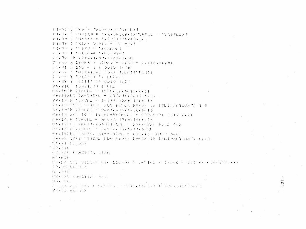
C, 1 7 = /J. j

; I 7A 1,7,12; = ! r '4; 4".t'd. L = ",1 75 1 = ,1/ Lys41.,,

IN k.,1 ", !

1.'1. 77 7 V ",4- I 'ir; ", !

1 7V 1! ( ) I '6 7, 1 1= tA;DN'v v 1157*',...1,./)1)

f.'1 = 1 ; Viii 1. z26(-P11 \ ! ! "

c I .1 t].) !

H. 111,16I: (--71,306. VJC LiN

VA. 6. 11, 11v 1E "i ;Kr-71H Cf. + V73. 16; (-

A. ( 1 I 1. )1,-, 1 6. 14, 1 z;

1 E Hr,,\Jt:1- ( ',74) 6. I 1 6, 6. 1 6

V 6.1 V VS -11' + (f013 6.,)1V 6.161 /4. V ) 6. 17, 6.(', A. 1 656 "-.64c,H L + 7 4: ; !-! '(."'

I ':`; C:! V 7. i) Iv, P-.): A. Hs.:1 '74 i Iur1.1iiL7L + 7. 6

f"..7,..-(q. It L% 1 .)\;1

V 1 V.

rj \.; ; :

si

Vf.i:'VL \... ( ) r, 1 1'V 7 i < '1'

V 7 7 1.

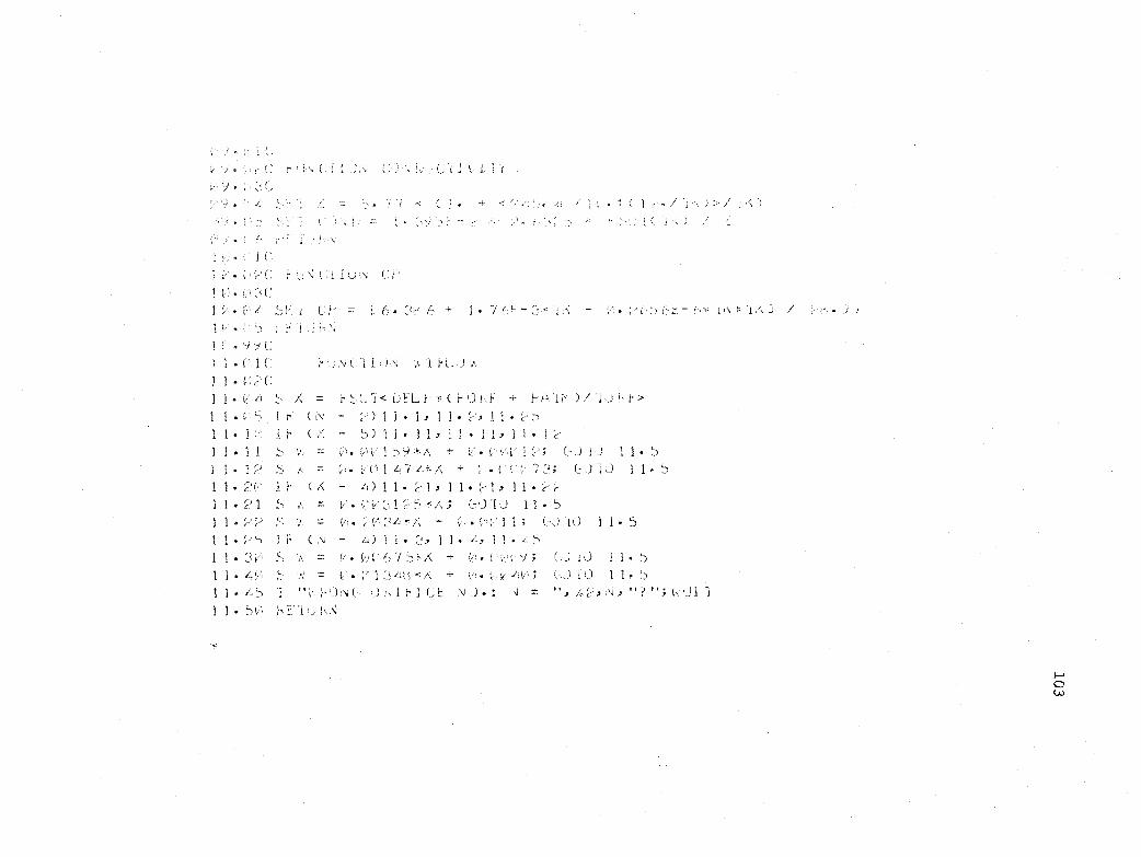
I.inrt\'2')/(7,1ICr-)

(117-)

ni

=

Yi

",)

c, 7I

II

:( N:)

cr7II

-)I)-

)JT.41,r7,_I,

v5.c:,/,(;) 11II(

)14 7,)1,

-),v1'.1.))=

)

N ))=

'4(4.I

Ic-,-/II

-;)7711

Ii

(7,,--;

H,i=t

(1),I I 1,),II(7Y)41;I

qTI+=c7;

c.;IIrIT-)f:';II.":),.,"!",,41-,(:...)',)=i1

-',111,II111111C(2,'')-1T.1i 11c-7;.IIc;II`1°11(;N-)./I-)I

4-41){ 714(1 >I_ "/=Y-7;v ,1II

)11

1.TI.)f\--I'1 I It.

(-

N'

?"/VT- zv----)tiU.4L:v;

1:INcH'U 1

1

(< (",°>±1)7

c/.)I..

I).".!

104

APPENDIX F

LEAKAGE ANALYSIS

105

LEAKAGE ANALYSIS

Leakage in the tubing, manometers, rotary union, etc., was

too low to be measured directly by the smallest orifice meter

available. Therefore an indirect means of.determining leak rate

was used, as follows:

The porous disk was removed, the therthowell placed up through

the rotating pipe was replaced with a slightly shorter one, and a

rubber stopper was inserted into the upper end of the rotating

pipe. Then the system was pressurized by opening the needle valve.

When the valve was closed, the mercury manometer measuring total

pressure in the system slowly fell, indicating some leakage of air

from the "closed" system. This test was repeated many times during

the development of the apparatus. Rotation of the pipe had no ap-

parent influence on the leak rate.

When plotted on semi-logarithmic paper, total pressure in the

system against time showed an exponential decay, as indicated in

Figure F-1. Due to subsequent leak testing and tightening of

fittings, etc., the data in the figure show a much greater slope

(more leakage) than those taken just before the heat transfer runs.

The latter data, however, showed such a slow decay that it was

difficult to ascertain the slope accurately. In the analysis that

follows, therefore, the data of Figure F-1 will be used as an upper

limit to the actual pressure decay.

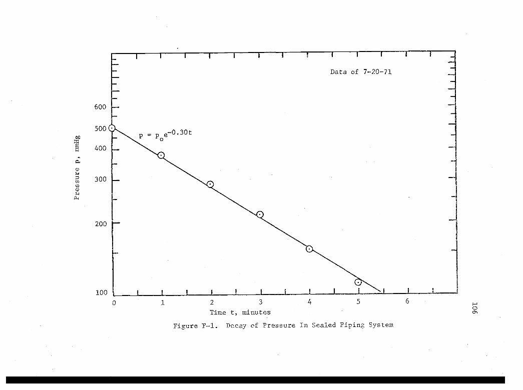
600

500

400

300

200

100

e-0.30t

Data of 7-20-71

0 1 2 3

Time t, minutes

4 5

Figure F-1. Decay of Pressure In Sealed Piping System

6

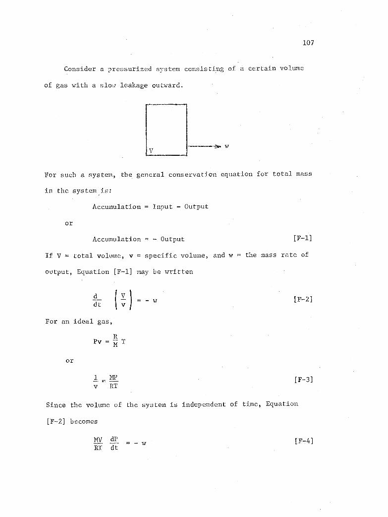
107

Consider a pressurized system consisting of a certain volume

of gas with a slow leakage outward.

For such a system, the general conservation equation for total mass

in the systemis:

Accumulation = Input - Output

Or

Accumulation = Output [F-1]

If V = total volume, v = specific volume, and w = the mass rate of

output, Equation [F-1] may be written

dt

IV

-V- ) "

For an ideal gas,

or

RPv = 1,7/ T

1 MP

v RT

[F-2]

[F-3]

Since the volume of the system is independent of time, Equation

[F-2] becomes

MV dP

RT dt w[F-4]

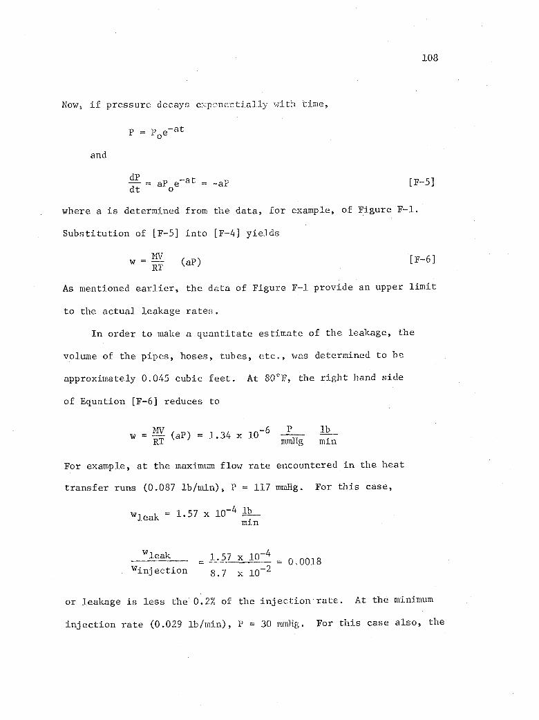
Now, if pressure decays exponentially with time,

and

p =P

-atO

dP

dt= aP

oe-at = -aP

where a is determined from the data, for example, of Figure F-1.

Substitution of [F-5] into [F-4] yields

NVw = (aP)RT

108

[F-6]

As mentioned earlier, the data of Figure F-1 provide an upper limit

to the actual leakage rates.

In order to make a quantitate estimate of the leakage, the

volume of the pipes, hoses, tubes, etc., was determined to be

approximately 0.045 cubic feet. At 80°F, the right hand side

of Equation [F-6] reduces to

P lw = NV (aP) = 1.34 x 10

-6

RT mmHg mibn

For example, at the maximum flow rate encountered in the heat

transfer runs (0.087 lb/min), P = 117 mmHg. For this case,

wleak 1.57 x 10-4 112__min

1.57 x 10-4= M018

. winjection 8.7 x 10-2

or leakage is less the 0.2% of the injection rate. At the minimum

injection rate (0.029 lb/min), P = 30 mmHg. For this case also, the

109

leakage is less than 0.2% of the injection rate. Because the

orifice calibration for measuring injection rate.were repro

ducible to 0.5%, and because the leakage calculated here is an

upper limit to the actual loss, it is concluded that leakage

rate makes a negligible contribution to the sources of error in

the heat transfer coefficients reported in this research.

110

APPENDIX G

NOMENCLATURE

111

NOMENCLATURE

Symbol Definition Units

B,B' constants used in Equations 4V74 and dimensionless

[V-4']

134- matching parameter used in Kays' work dimensionless

C,C' constants used in Equations [V74] and dimensionless[v -4']

Cf

friction coefficient dimensionless

Cp heat capacity BTU/lb °F

D diameter of disk ft

D diffusivity ft2/hr

D damping factor in mixing length ex- dimensionlesspression

F dimensionless radial velocity dimensionless

g gravitational acceleration0 ft/hr2

G dimensionless angular velocity dimensionless

Gr Grashof number, SgR3 (Tw - T.)/v2 dimensionless

h heat transfer coefficient BTU/hr ft2 °F

H enthalpy BTU/lb

H clearance, distance from disk to stationary ft

surface opposite

H dimensionless axial velocity dimensionless

k thermal conductivity BTU/hr ft °F

Q Prandtl mixing length ft

M molecular weight lb/lb mole

n mass flux lb/min ft2

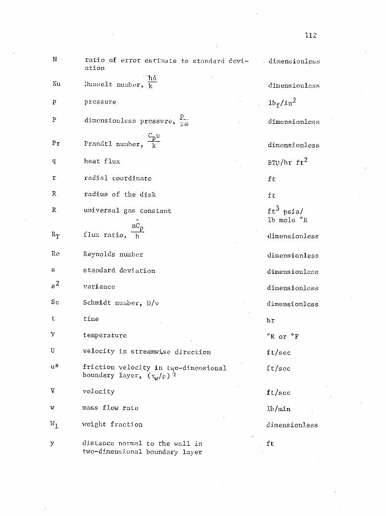
112

N ratio of error estimate to standard devi- dimensionlessation

h(S-

Nu Nusselt number, k dimensionless

p pressure lbf/in2

P dimensionless pressure, dimensionless

Pr Prandtl number, k dimensionless

q heat flux BTU/hr ft2

radial coordinate ft

R radius of the disk ft

R universal gas constant ft3 psia/lb mole °R

nCp

RT flux ratio, h dimensionless

Re Reynolds number dimensionless

s standard deviation dimensionless

s2 variance dimensionless

Sc Schmidt number, D/v dimensionless

t time hr

T temperature °R or °F

U velocity in streamwi.se direction ft/sec

u* friction velocity in too- dimensional ft/secboundary layer, (Tw/p)-a

V velocity ft/sec

w mass flow rate lb/min

141 weight fraction dimensionless

y distance normal to the wall in ft

two-dimensional boundary layer

113

y.non-dimensionalized value of y, v . dimensionless

z axial coordinate ft

temperature coefficient of volume ex- °R-1pension

boundary layer thickness, (v/w) 2 ft

A estimated uncertainty dimensionless

emissivity dimensionless

dimensionless distance normal to the dimensionlessdisk, z/6

6 angular coordinate radians

T - T.dimensionless temperature ratio, dimensionless

Tratio of heat transfer coefficientwith dimensionlessinjection to heat transfer coefficientwithout injection, h/ho

P viscosity lb/ft hr

v kinematic viscosity ft2/hr

P density lb /f t3

a Stefan-Boltzmann constant BTU/hr ft2 °R4

Z summation, total dimensionless

shear stress lbf/ft2

dimensionless ratio of weight dimensionlessfractions, W, Wi.

Wiw

angular velocity sec-1

114

Subscripts Definition

cony convection

corr corrected

e in external flow of two-dimensional boundarylayer

o zero injection

o orifice meter

rad radiation

w evaluated at the wall or disk surface

woo evaluated on the surface of the surroundings,far from the disk

x using distance along the surface for a typicallength in a dimensionless group

00 evaluated in the fluid, far from the disk surface

Superscripts

per lb

ti per mole