Embed Size (px)
Citation preview
Euro. Jnl of Applied Mathematics (2003), vol. 14, pp. 613–636. c© 2003 Cambridge University Press
DOI: 10.1017/S0956792503005291 Printed in the United Kingdom613
Transport equations with resting phases
T. HILLEN
Department of Mathematical and Statistical Sciences, University of Alberta,
Edmonton T6G 2G1, Canada
(email: [email protected])
(Received 21 August 2002; revised 12 May 2003)
We study a transport model for populations whose individuals move according to a velocity
jump process and stop moving in areas which provide shelter or food. This model has direct
applications in ecology (e.g. homeranges, territoriality, stream ecosystems, travelling waves)
or cellular biology (e.g. movement of bacteria or movement of proteins in the cell nucleus).
In this paper we consider a general model from a mathematical point of view. This provides
general insight into the features of these models, which in turn is useful in the modelling
process. We consider a singular perturbation expansion and show that the leading order term
of the outer solution satisfies a reaction-advection-diffusion equation. The advective term
describes taxis toward homeranges or toward regions of shelter. The reaction terms are given
by “effective” birth and death rates. Within this framework, the parameters of the reaction-
advection-diffusion model (like mobility, drift, birth or death rates) are directly related to the
individual movement behaviour of the species at hand (like velocity, frequency of directional
changes, response to spatial in-homogeneities, death, or reproduction). We prove that in a
homogeneous environment the diffusion limit approximates the solution of the resting-phase
transport model to second order in the perturbation parameter.
1 Introduction
A widely used class of mathematical models to describe spatial spread of growing
populations are reaction-diffusion models (e.g. see Murray [18] or Britton [4]). They are
based on an uncorrelated random walk (Brownian motion) and they assume instantaneous
birth, neglecting resting periods due to birth events.
The assumption of uncorrelated random walk has been extended to models which are
based on correlated random walk and which lead to transport equations (e.g. Stroock [23],
Alt [1], Othmer et al. [19], Hadeler [11], Dickinson [10], Hillen & Othmer [13, 20]). The
parameters for transport models are mean speed, mean turning rates and turning-angle
distribution: parameters which can be measured from the movement paths of individuals.
For that reason the transport models are more closely related to the natural process
than the diffusion-based models. In fact, using appropriate scaling analysis, the transport
model leads to reaction-diffusion models. In particular, in Hillen & Othmer [13], a theory
has been introduced to obtain the parabolic limit of a transport model in a general and
transparent way.
In this paper, we extend the modelling with transport equations to include periods of
resting where the individuals do not move. The reasons are manifold and range from
shelter, den sites, or nests, to hunting spots, or feeding grounds. We give examples below.

614 T. Hillen
Since the decision when to move and when to rest is an individual one, it is natural to
study this dynamic in the framework of transport models (rather than diffusion models).
In Othmer & Hillen [20] a resting-phase transport model with constant stopping rates
was already formulated. In this paper we extend that model to include spatially variable
stopping rates (inhomogeneous environment) and we give proofs for the various results
(which are not contained in Othmer & Hillen [20]).
The model presented here combines a transport model for correlated random walk
with resting periods on preferred locations. Using a singular perturbation analysis it is
shown that the long time asymptotics (i.e. outer solution) are described by a reaction-
advection-diffusion model. It appears that the diffusion coefficient is proportional to the
mean fraction of the population which is moving and the birth term is proportional to
the mean fraction of resting particles. The spatial non-homogeneities lead to a drift term
toward preferred areas.
Typically, reproductions and deaths occur on a slower time scale than the random
walk. The ratio of these two corresponding time scales defines a small parameter (ε). A
singular perturbation analysis leads to reaction-advection-diffusion equations (parabolic
limit). We show that the inner solution relaxes to a homogeneous distribution and that the
outer expansion is well described by a reaction-advection-diffusion model with effective
birth and death rates. We match inner and outer expansions and we prove that, in the
spatial homogeneous case with linear birth and death rates, the long time asymptotics are
approximated by the outer expansion to second order in the perturbation parameter. We
discuss various special cases, which include small perturbations to homogeneous initial
conditions, the case of large or small fraction of resting particles and we compare the
results to a resting-phase diffusion model.
1.1 Applications
Models for movement including resting-phases are relevant in ecology and also in cellular
biology:
Recent studies of stream ecosystems use reaction-diffusion models to investigate the drift
paradox [17, 21]. The drift paradox occurs for aquatic insects, like the Baetidis mayflies
and stoneflies, who occur as persistent populations in streams. The larvae are relatively
immobile on the bottom of the stream (resting), while the adults are able to swim and
as they rise from the bottom they are transported downstream. Although individuals are
drained from that location, the population as a whole remains persistent (drift paradox).
The inclusion of moving-resting dynamics, as in Pachepsky et al. [21] sheds a new light
on possible resolutions of the drift paradox.
The dynamics of oriented movement (searching) and resting is also important to
understand the survival of endangered species in fragmented habitats. In Carroll &
Lamberson [6] the territoriality of spotted owls was studied. In their model the juvenile
owls are assumed to search for suitable territories (moving), while the adults have already
occupied a suitable territory (resting). Carroll and Lamberson study a compartmental
model of habitat clusters, which does not include any spatial information. To include the
given landscape in a model, a transport model, like the one studied here, would be a
natural starting point.

Transport equations with resting phases 615
Another application of a similar nature occurs for modelling the formation of hom-
eranges. Homeranges provide shelter and include feeding grounds. In many cases they
include a den site for resting and reproduction. Homeranges for wolves have been studied
by Briscoe et al. [3] without inclusion of resting phases. There the formation of hom-
eranges was triggered by scent marking. It would be interesting to see the influence of
resting-moving dynamics on the home range formation.
Lewis & Schmitz [16] and Hadeler & Lewis [12] study the effect of resting-moving
dynamics on the invasion of microbes. Certain microbes reproduce while they are sta-
tionary and only when they are not reproducing they can be spread spatially by wind or
by water. In both papers a resting-phase Fisher model is investigated, which divides the
whole population into a moving part, which does not reproduce, and a resting part, which
only can reproduce. The model of Lewis et al. is a special case of the model studied here.
In collaboration with J. Muller, we are currently investigating homeranges of bats.
The movement of individual bats shows interesting interactions of moving and resting
dynamics. In detailed studies the movement path’s of ten individual bats has been recorded.
From this data set we plan to estimate mean speed, turning rates, turn-angle distributions
and spatially dependent stopping rates.
In collaboration with M. Lewis and J. M. Lee, we are currently working on an model
for prey-taxis. The predator stops movement at locations with high prey density. This
process in turn leads to prey-taxis in the parabolic limit [14].
A totally different application occurs for the movement of proteins in the cell nucleus. In
fluorescence-recovery-after-photobleaching experiments it was shown that certain proteins
in the cell nucleus show movement patterns which cannot be described by simple diffusion.
In Carrero et al. [5] a resting-phase diffusion model was used to successfully analyze the
fluorescence recovery curves. In addition, with use of this model it is possible to predict
the average number of bound (=resting) proteins. This information cannot be directly
determined in experiments.
Cosner & Lou [8] and Belgacem & Cosner [2] consider a reaction-diffusion model with
drift toward better environments. They study the benefit for populations which use this
strategy. In fact, their model is a special case of the parabolic limit equation derived here
(3.14). In Cosner et al., the modelling of the corresponding drift term is done ad hoc. The
asymptotic scaling analysis as done here relates the drift mechanism to individual move-
ment behaviour and it gives an a posteriori justification of the model used by Cosner et al.
1.2 The model
To model a population whose members are moving according to a correlated random walk
and which rest occasionally, we split the total population density N(t, x) into a density
p(t, x, v) of individuals moving with velocity v ∈ V and a density r(t, x) for particles resting
at x ∈ Ω. The velocity set V is assumed to be bounded with ω = |V | and symmetric of
the form that v ∈ V implies −v ∈ V . We study a model for (p, r) which is based on the
following assumptions:
(1) The pure movement process is a velocity jump process
pt + v · ∇p = −µp+ µ
∫V
T (v, v′)p(., ., v′) dv′. (1.1)

616 T. Hillen
We assume that the kernel T (v, v′) satisfies the following basic assumptions (T1)–
(T4), which were first introduced in Hillen & Othmer [13]:
(T1) T (v, v′) 0,∫VT (v, v′) dv = 1, and
∫V
∫VT 2(v, v′) dv′ dv < ∞.
(T2) There exist some u0 0 with u0 0, some integer N and a constant ρ > 0
such that for all (v, v′) ∈ V × V
u0(v) TN(v′, v) ρu0(v),
where the Nth iterate of T is
TN(v, v′) :=
∫. . .
∫T (v, w1)T (w1, w2) · · ·T (wN−1, v
′) dw1 . . . dwN−1.
(T3) We introduce an integral operator T by
Tp =
∫V
T (v, v′)p(v′) dv
and we assume that ‖T‖〈1〉⊥ < 1, where 〈1〉⊥ denotes the orthogonal com-
plement of the subspace 〈1〉 ⊂ L2(V ) of functions constant in v.
(T4)∫VT (v, v′) dv′ = 1.
(2) There is a spatially dependent rate α(x) > 0 such that individuals stop moving at
location x with that rate α(x).
(3) At rest particles give birth at a rate g(N) 0 (g for ‘gain’).
(4) Individuals start moving with constant rate β > 0 and they choose a direction with
equal distribution on V .
(5) Death occurs for moving and resting particles at the same rate l(N) 0. (l for
‘loss’).
We denote the turning operator as L := −µ(I − T) and Proposition 1.1 of Hillen &
Othmer [13] applies:
Proposition 1.1 Assume (T1)–(T4). Then
(1) 0 is a simple eigenvalue of L with eigenfunction φ(v) ≡ 1.
(2) There exists an orthogonal decomposition L2(V ) = 〈1〉 ⊕ 〈1〉⊥, and for all ψ ∈ 〈1〉⊥
we have ∫ψLψ dv −ν2‖ψ‖2
L2(V ), with ν2 ≡ µ(1 − ‖T‖〈1〉⊥
).
(3) Each eigenvalue λ 0 satisfies −2µ < Re λ −ν2 < 0, and there is no other positive
eigenfunction.
(4) ‖L‖L(L2(V ),L2(V )) 2µ.

Transport equations with resting phases 617
(5) L restricted to 〈1〉⊥ ⊂ L2(V ) has a linear inverse F with norm
‖F‖L(〈1〉⊥ ,〈1〉⊥) 1
ν2.
The resting-phase transport model reads
pt + v · ∇p = Lp− α(x)p+β
ωr − l(N)p (1.2)
rt = α(x)
∫V
p(., ., v) dv − βr + g(N)r − l(N)r, (1.3)
where the total particle density N is given by
N(t, x) =
∫V
p(t, x, v) dv + r(t, x).
We assume compactly supported initial data on Ω = IRn, which are L2-integrable on
IRn × V . Then the solution will have compact support as long as it exists. Note that the
velocity v appears as a parameter in (1.2). Hence, no conditions on ∂V are required.
For later use we define the pure kinetic birth-death process without any movement by
u = f(u) := g(u)u− l(u)u.
We study the parabolic limit of (1.2), (1.3) in the framework of singular perturbation
theory and matching asymptotic expansions. For that purpose we identify appropriate
scalings of space and time (parabolic scaling). As pointed out in Hillen & Othmer [13],
these scalings occur quite naturally for biological populations. For a given small quantity
ε > 0 we consider fast and slow time scales, t and τ = ε2t, respectively, on microscopic and
macroscopic space scales x and ξ = εx, respectively. In singular perturbation theory one
splits the dynamics into two parts. The first part (inner solution) describes the relaxation
of the initial data on the fast time scale t. The outer solution describes the long time
behaviour on the slow time scale τ. The initial data for the outer solution are not directly
specified by the initial data of the original problem (1.2), (1.3). This can be achieved by
matching inner and outer expansions in an intermediate region. Roughly speaking, the
asymptotics of the inner solution for t → ∞ defines the initial condition for the outer
solution at τ = 0.
We begin with local and global existence of solutions to (1.2), (1.3). Then we study
the outer solution (p, r) which leads to the diffusion limit equation (3.14). This gives
approximations of second order in the perturbation parameter ε (Theorem 5.5). After
that, we study the inner solution and we illustrate that both parts match correctly.
2 Assumptions, existence, positivity
Here we collect a set of basic assumptions which we use throughout the paper.
(A1) f ∈ C1(IR), g, l ∈ C1b (IR) and l(N∗) g(N∗) for some N∗ > 0.
(A2) The initial data
p(0, x, v) = ϕ(x, v) 0, r(0, x) = ψ(x) 0

618 T. Hillen
are spatially compact supported with∫ϕ(x, v) dv + ψ(x) N∗, ϕ(x, .) ∈ L2(V ) for
all x ∈ IRn and ϕ(., v) ∈ C0,σ(IRn) for almost all v ∈ V and some 0 < σ < 1.
(A3) α(x) > 0, and α ∈ H1(IRn) ∩W 1,∞(IRn).
(A4) V = sSn−1 or V = Bs(0) for some s > 0, and ω = |V |.(A5) T > 0 is fixed.
The assumption (A5) is not important for our existence result. But the assumption will
be used for the approximation estimates later. Hence we choose to state it here together
with the other assumptions.
First we show global existence:
Theorem 2.1 Assume (T1)–(T4) and (A1)–(A4). For each pair of initial data ϕ,ψ with
ϕ ∈ D(Φ) and ψ ∈ L2(IRn) with ϕ(., v), ψ ∈ L1(IRn) there is a unique solution (p, r) of (1.2),
(1.3) with
p ∈ C1([0,∞), L2(IRn × V )) ∩ C0([0,∞), D(Φ)), r ∈ C1([0,∞), L2(IRn))
and p(0, .) = ϕ and r(0) = ψ, where Φ is the shift operator as defined below.
Proof We collect a number of arguments and apply standart semigroup theory:
(1) The shift operator Φ = −v · ∇ with domain
D(Φ) = ϕ ∈ L2(IRn × V ) : ϕ(., v) ∈ H1(IRn)
generates a strongly continuous, positive, unitary group of translations on L2(IRn ×V ) (see also Dautray & Lions [9, Ch XXI, Sect. 2, Prop 1]).
(2) The nonlinearities are of the form g(ϕ)ψ, l(ϕ)ψ with ϕ,ψ ∈ L2(IRn × V ) with
bounded and differentiable rates g and l. Hence g(ϕ)ψ, l(ϕ)ψ ∈ L2(IRn × V ).
Moreover, the mappings ((ϕ,ψ) → g(ϕ)ψ) and ((ϕ,ψ) → l(ϕ)ψ) are globally
Lipschitz continuous on both L2(IRn × V )2 and H1(IRn × V )2.
(3) With α given as in (A3) also the mappings p → α(x)p, and p → α(x)∫p dv are
Lipschitz continuous on both spaces L2(IRn × V )2 and H1(IRn × V )2.
(4) The turning operator L is linear and compact.
Hence local and global existence of solutions to (1.2, 1.3) follows from standard Perron-
iteration and perturbation arguments (e.g. see Taylor [24] or Pazy [22]).
System (1.2), (1.3) also preserves positivity:
Lemma 2.2 Under the assumptions of the previous Theorem we have
p(t, x, v) 0 and r(t, x) 0.
Proof If we assume that the solution (p(t), r(t)) becomes negative somewhere then there
is a first time t0 where either p(t0) = 0, or r(t0) = 0, or both.

Transport equations with resting phases 619
In the first case, p(t0) = 0, we find for t = t0 from (1.2) that
pt + v · ∇p =β
ωr 0.
In the second case, r(t0) = 0, we find from (1.3) that at t = t0
rt = α(x)
∫V
p(., ., v) dv 0.
Note that Φ = −v · ∇ generates a positive group of translations. Hence in both cases p(t),
or r(t) cannot decay below 0.
3 The outer expansion
3.1 Scaling
In Hillen & Othmer [13] we introduced the scaling of
τ = ε2t, ξ = εx,
for small 0 < ε 1.
We assume that there is a large number of individual directional changes per birth or
death event. This means that birth and death events occur on a much slower time scale
than the random walk process. As t denotes the fast time scale (as for the random walk)
and τ denotes the slow time scale we assume that the pure kinetics is described by
uτ = f(u),
or equivalently
ut = ε2f(u).
We identify as follows:
f(u) = ε2f(u) = ε2(g(u)u− l(u)u).
System (1.2), (1.3) in the new variables (τ, ξ) reads
ε2pτ + εv · ∇ξp = Lp− αp+β
ωr − ε2 l(N)p (3.1)
ε2rτ = α
∫p(., ., v) dv − βr + ε2g(N)r − ε2 l(N)r, (3.2)
where p(τ, ξ, v) = p(τ/ε2, ξ/ε, v), r(τ, ξ) = r(τ/ε2, ξ/ε), and α(ξ) = α(ξ/ε). We consider series
expansions in ε up to order k > 2:
p(τ, ξ, v) :=
k∑j=0
εjpj(τ, ξ, v), r(τ, ξ) :=
k∑j=0
εjrj(τ, ξ)
N(τ, ξ) :=
k∑j=0
εjNj(τ, ξ), Nj(τ, ξ) = rj(τ, ξ) +
∫V
pj(τ, ξ, v) dv, 0 j k.

620 T. Hillen
We expand the nonlinearities g, l according to this representation:
g(N) = g(N0) + g′(N0)
k∑
j=1
εjNj
+ l.o.t.
l(N) = l(N0) + l′(N0)
k∑
j=1
εjNj
+ l.o.t..
3.2 Formal derivation of the diffusion limit
We introduce all of the above expansions into system (3.1), (3.2) and collect orders of ε.
During this section we neglect the subscript ξ at the ∇-operator:
ε0 :
0 = Lp0 − αp0 + β
ωr0
0 = α∫p0 dv − βr0
(3.3)
ε1 :
v · ∇p0 = Lp1 − αp1 + β
ωr1
0 = α∫p1 dv − βr1
(3.4)
ε2 :
p0,τ + v · ∇p1 = Lp2 − αp2 + β
ωr2 − l(N0)p0
r0,τ = α∫p2 dv − βr2 + g(N0)r0 − l(N0)r0.
(3.5)
From (3.3) it follows that
r0 =α
β
∫p0 dv.
Hence the first equation of (3.3) reads
0 = Lp0 − αp0 +α
ω
∫p0 dv =: Lαp0, (3.6)
where the operator Lα(ξ) is given for α(ξ) > 0 and ψ ∈ L2(V ) by
Lα(ξ)[ψ(v)] = −(µ+ α(ξ))ψ(v)
+ (µ+ α(ξ))
∫V
(µ
µ+ α(ξ)T (v, v′) +
α(ξ)
(µ+ α(ξ))ω
)ψ(v′) dv′. (3.7)
We denote the modified turning kernel by
Tα(ξ, v, v′) :=
µ
µ+ α(ξ)T (v, v′) +
α(ξ)
(µ+ α(ξ))ω(3.8)
and Tα is the integral operator defined by Tα. For α =constant the formula for Lα and
Tα were already given in Othmer & Hillen [20].
Lemma 3.1 For each ξ ∈ IRn the kernel Tα satisfies conditions (T1)–(T4).
Proof Since T is assumed to satisfy (T1)–(T4) it satisfies T 0. Hence, for α(ξ) > 0 we
have Tα(ξ, v, v′) > 0 for all (v, v′) ∈ V 2. Then (T2) and the first condition of (T1) follow.

Transport equations with resting phases 621
Integration of the kernel gives:
∫Tα(ξ, v, v
′) dv =µ
µ+ α(ξ)+
α(ξ)
µ+ α(ξ)= 1 =
∫Tα(ξ, v, v
′) dv′.
Hence (T4) and the second condition in (T1) are satisfied. Moreover
∫ ∫T 2α (ξ, v, v′) dv dv′ =
(µ2
∫ ∫T 2(v, v′) dv dv′ + 2µα(ξ) + α(ξ)2
)(µ+ α(ξ))−2 < ∞.
Then (T1) is satisfied as well and it remains to check (T3):
‖Tα‖〈1〉⊥ = supψ∈L2(V ),‖ψ‖=1,
∫ψ dv=0
∣∣∣∣∫
µ
µ+ α(ξ)T (v, v′)ψ(v′) dv′ +
α(ξ)
(µ+ α(ξ))ω
∫ψ(v) dv
∣∣∣∣ ‖T‖〈1〉⊥ < 1.
Hence Proposition 1.1 applies for Lα(ξ), and we have the following properties.
Corollary 3.2 Assume (T1)–(T4) for T (v, v′) and let Lα(ξ) be defined by (3.7) for α > 0.
Then for each ξ ∈ IRn
(1) 0 is a simple eigenvalue of Lα(ξ) and the corresponding eigenfunction is φ(v) ≡ 1.
(2) There is a decomposition L2(V ) = 〈1〉 ⊕ 〈1〉⊥ and for all ψ ∈ 〈1〉⊥
∫ψLα(ξ)ψ dv −να(ξ)‖ψ‖2
L2(V ), where να(ξ) ≡ (µ+α(ξ))(1−‖Tα‖〈1〉⊥). (3.9)
(3) All nonzero eigenvalues λ satisfy −2(µ + α(ξ)) < Re λ −να(ξ) < 0, and to within
scalar multiples there is no other positive eigenfunction.
(4) ‖Lα(ξ)‖L(L2(V ),L2(V )) 2(µ+ α(ξ)).
(5) Lα(ξ) restricted to 〈1〉⊥ ⊂ L2(V ) has a linear inverse Fα(ξ) with norm
‖Fα(ξ)‖L(〈1〉⊥ ,〈1〉⊥) 1
να(ξ). (3.10)
Now we go back to consider the εj-systems for j = 0, 1, 2.
ε0 : With the above Corollary it follows from (3.6) that p0 = p0(τ, ξ) does not depend on
velocity v ∈ V . Then
r0 =α
β
∫p0 dv =
αω
βp0. (3.11)
ε1 : From the second equation of (3.4) it follows that r1 = α/β∫p1 dv, hence in the first
equation of (3.4) the operator Lα appears again:
v · ∇p0 = Lαp1.

622 T. Hillen
This equation is solvable since
∫(v · ∇p0) dv =
∫v dv · ∇p0 = 0.
Then
p1 = Fα(v · ∇p0), with Fα :=(Lα|〈1〉⊥
)−1. (3.12)
Since Fα is one-to-one on 〈1〉⊥ we have∫p1 dv = 0 and then r1 = 0.
ε2 : From the second equation of (3.5) we obtain
β
ωr2 =
1
ω
(α
∫p2 dv + g0r0 − l0r0 − r0,τ
),
where for now we write g0 := g(N0) and similarly for l0. With (3.11) we get
β
ωr2 =
α
ω
∫p2 dv +
α
β(g0p0 − l0p0 − p0,τ).
We introduce this expression into the first equation of (3.5):
p0,τ + v · ∇p1 = Lαp2 +α
β(g0 − l0)p0 − α
βp0,τ − l0p0. (3.13)
The solvability condition with respect to Lα reads, with use of (3.12),
∫V
(1 +
α
β
)p0,τ dv + ∇ ·
∫V
vFαv dv∇p0 =α
β(g0 − l0)
∫V
p0 dv − l0
∫V
p0 dv.
Since p0 does not depend upon velocity v ∈ V this equation becomes
ω
(1 +
α
β
)p0,τ + ∇ ·
∫V
vFαv dv · ∇p0 = g0α
βωp0 − l0
(1 +
α
β
)ωp0.
Now g0 = g(N0) and
N0 = r0 + ωp0 =
(1 +
α
β
)ωp0.
Finally, we write the above equation as an equation for N0. Note that the ∇p0-term
produces an additional drift term, since α depends on space ξ. The parabolic limit
equation reads
N0,τ = ∇(Dα,β(ξ)∇ N0 − Dα,β(ξ)
N0∇α(ξ)β + α(ξ)
)+
α(ξ)
α(ξ) + βg(N0)N0 − l(N0)N0 (3.14)
with diffusion tensor
Dα,β(ξ) := − β
ω(α(ξ) + β)
∫vFα(ξ)v dv. (3.15)
Remark 3.3 (1) Due to the non-homogeneous environment we obtain a taxis term in
direction of −∇α. The population moves toward regions of high stopping probability,

Transport equations with resting phases 623
which reflects shelter and safe environment near the den sites or homeranges. This
gives an a posteriori justification for a model studied by Cosner & Lou [8], who
directly assume taxis toward favorable environments.
(2) We obtain a birth rate reduced by a factor α(ξ)/(α(ξ) + β). This factor describes
the mean fraction of the population at a location ξ, which is at rest at any time.
(3) It turns out that, in general, we obtain non-isotropic diffusion. The diffusion tensor
is scaled by a factor β/(α(ξ) + β), which describes the mean proportion of moving
particles at location ξ. In § 6 we will discuss special cases for the diffusion tensor
Dα,β .
4 Inner expansion and matching
For the inner expansion we consider the original fast time scale t and the macroscopic
space scale ξ. Then p(t, ξ, v) = p(t, x/ε, v) and r(t, ξ) = r(t, x/ε) satisfy the initial value
problem
pt + εv · ∇p = Lp− αp+ βωr − ε2 l(N)p
rt = α∫p dv − βr + ε2g(N)r − ε2 l(N)r
p(0, ξ, v) = ϕ(ξ/ε, v) r(0, ξ) = ψ(ξ/ε),
(4.1)
where N =∫p dv + r and l(N) = l(N(ε2t, ξ)) and g(N) = g(N(ε2t, ξ)).
Again, we study expansions in ε
p(t, ξ, v) :=
k∑j=0
εj pj(t, ξ, v), r(t, ξ) :=
k∑j=0
εj rj(t, ξ)
N(t, ξ), :=
k∑j=0
εjNj(t, ξ), Nj(t, ξ) = rj(t, ξ) +
∫pj(t, ξ, v) dv, 0 j k,
and we collect orders of ε of order zero only:
ε0 :
p0,t = Lp0 − αp0 + β
ωr0
r0,t = α∫p0 dv − βr0
. (4.2)
We show that the functional
E(p, r) :=ω
2
∫V
p2 dv + r
∫V
p dv +r2
2
is a Lyapunov function of the integro-differential system (4.2). Note that E is bounded
below by 0, since the solutions are non-negative (Lemma 2.2).
Theorem 4.1 For solutions (p0, r0) of (4.2) we have
d
dtE(p0, r0) −αω
∫ (p0 − 1
ω
∫p0 dv
′)2
dv.

624 T. Hillen
Proof
d
dt
ω
2
∫p2
0 dv = ω
∫p0Lp0 dv − ωα
∫p2
0 dv + β
∫p0 dv r0
−αω∫p2
0 dv + βr0
∫p0 dv
d
dt
(r0
∫p0 dv
)=
(α
∫p0 dv − βr0
) ∫p0 dv + r0
(∫Lp0 dv − α
∫p0 dv +
β
ω
∫r0 dv
)
= α
(∫p0 dv
)2
− (α+ β)r0
∫p0 dv + βr20 ,
d
dt
r202
= αr0
∫p0 dv − βr20 .
From these inequalities it follows that
d
dtE(p0, r0) −ωα
∫p2
0 dv + α
(∫p0 dv
)2
= −αω∫ (
p0 − 1
ω
∫p0 dv
′)2
dv.
For now we abbreviate the mean value by
φ0(t, ξ) :=
∫p0(t, ξ, v
′) dv′.
Since E is a Lyapunov function we have
limt→∞
∥∥∥∥p0(t, ξ, .) − 1
ωφ0(t, ξ)
∥∥∥∥2
= 0.
Hence in the limit of τ → ∞ the function p0 does not depend on v. Then Lp0 = 0 and
the asymptotic behaviour of (4.2) is determined by the system
φ0,t = −αφ0 + βr0(4.3)
r0,t = αφ0 − βr0.
The mass N(ξ) = φ0(ξ) + r0(ξ) is preserved for all ξ ∈ IRn and the steady state (βN/(α+
β), αN/(α+ β)) is asymptotically stable. The initial data
p(0, ξ, v) = ϕ(ξ, v), r(0, ξ) = ψ(ξ)
determines N as
N(ξ) =
∫ϕ(ξ, v) dv + ψ(ξ).

Transport equations with resting phases 625
Hence the limit of the inner solution (p0, r0) for t → ∞ is given by
P0(ξ) =β
ω(α(ξ) + β)
(∫ϕ(ξ, v′) dv′ + ψ(ξ)
)(4.4)
R0(ξ) =α(ξ)
α(ξ) + β
(∫ϕ(ξ, v′) dv′ + ψ(ξ)
). (4.5)
Matching: to match inner and outer solutions we use the asymptotic limit of the inner
solution (4.4, 4.5) as initial condition for the outer solution. These are homogeneous in
v, as was expected for the outer solution. The corresponding initial condition for the
parabolic limit N0(τ, ξ) is then given by
N0(0, ξ) = ωP0(ξ) + R0(ξ) =
∫V
ϕ(ξ, v) dv + ψ(ξ). (4.6)
This matches exactly the initial conditions of the outer expansion which we used in (5.4).
5 Spatially homogeneous environment
In this section we consider the case of α(x) = α= constant in more detail. We prove that
the outer solution provides a good approximation. The approximation is of order ε2 in
intervals of the form θ/ε2 < t T/ε2 on compact sets Ω ⊂ IRn.
First we show a global L2-estimate for p0. For that purpose we need some information
on mean values of p. Let
p(t, x) :=
∫p(t, x, v) dv p(t) :=
∫p(t, x) dx,
r(t) :=
∫r(t, x) dx, N(t) :=
∫N(t, x) dx = p(t) + r(t).
(5.1)
Lemma 5.1N(t) N(0)e‖g‖∞t. (5.2)
Proof Integration of system (1.2, 1.3) with respect to space and velocity gives
pt = −αp+ βr −∫l(N)p dx
rt = αp− βr +
∫g(N)r dx−
∫l(N)r dx.
(5.3)
Note that due to∫T (v, v′) dv = 1 the V -integral of Lp vanished. The above equations
add to
Nt =
∫g(N)r dx−
∫l(N)(r + p) dx.
where the last term is non-positive. Then Nt ‖g‖∞N and we obtain (5.2).
Proposition 5.2 Assume (A1)–(A5). Let (p, r) denote a solution of (1.2), (1.3). Then for each
t with 0 < t T there is a constant c1 = c1(α, β, ω, µ,minl, ‖g‖∞, T ) such that
‖p(t, ., .)‖L2(IRn×V ) c1N(0).

626 T. Hillen
Proof With use of (1.2) we obtain
d
dt
1
2
∫p2 dv =
∫p
(−v · ∇p+ Lp− αp+
β
ωr − l(N)p
)dv
= −∇ · 1
2
∫vp2 dv +
∫pLp dv − α
∫p2 dv +
β
ω
∫p dv r − l(N)
∫p2 dv.
In view of the inequality∫pLp dv 0 (see Proposition 1.1), integration of the equation
above with respect to space gives
d
dt
1
2‖p‖2
L2(IRn×V ) −α‖p‖2L2(IRn×V ) +
β
ωN2 − minl‖p‖2
L2(IRn×V ).
Here we used Lemma 5.1 and the fact that∫(∫p dv r) dx N2. With use of Gronwall’s
Lemma and Lemma 5.1 the assertion follows.
5.1 Regularity properties of the limit equation
Here we study regularity properties of the parabolic limit initial value problem in case of
α = const.
N0,τ = ∇Dα,β∇N0 + αα+ β
g(N0)N0 − l(N0)N0,
N0(0, ξ) =∫ϕ(ξ, v) dv + ψ(ξ).
(5.4)
Lemma 5.3 The interval Γ := [0, N∗] is positively invariant for solutions of (5.4).
Proof A result of Chuey et al. [7] applies.
Proposition 5.4 For ϑ with 0 < ϑ < T we have
(i) supϑτT
‖D2N0(τ, .)‖∞ Kϑ,T‖N0(0, .)‖C0,σ ,
(ii) supϑτT
‖N0,τ(τ, .)‖∞ κα,βKϑ,T‖N0(0, .)‖C0,σ + c3N∗,
where
Kϑ,T = c2(ϑσ/2−1 + Tσ/22[2TK1(N
∗)]+1).
c3 =α
α+ β‖g‖C0(Γ ) + ‖l‖C0(Γ )
κα,β =βs2
ω(α+ β)να,
c2 is defined by (5.5) and K1(N∗) is given by (5.9).
Proof Since A := ∇Dα,β∇ defines a strongly elliptic sectorial operator (see Hillen &
Othmer [13, Lemma 3.3]) it generates an analytic contraction semigroup on C2+σ(IRn)
([15]). Moreover, for φ ∈ C0,σ(IRn), which does not grow faster than ec|x|2 for |x| → ∞, we

Transport equations with resting phases 627
have the regularity property that
‖D2(eAτφ)‖∞ c2τσ/2−1‖φ‖C0,σ (5.5)
(See Ladyzhenskaja et al. [15, Chapt. IV, 11 formula (11.6)]). Note that for compactly
supported initial data the solutionN0(τ, ξ) of (5.4) has exactly the correct growth behaviour
as |x| → ∞. This can be seen by representing the solution with fundamental solutions
[15]. From the limit equation (5.4) we obtain
N0(τ, ξ) = eAτN0(0, ξ) +
∫ τ
0
eA(τ−θ)(
α
α+ βg(N0)N0 − l(N0)N0
)dθ (5.6)
which leads to
‖N0(τ, .)‖C0,σ ‖N0(0, .)‖C0,σ +
∫ τ
0
∥∥∥∥ α
α+ βg(N0)N0 − l(N0)N0
∥∥∥∥C0,σ
dθ. (5.7)
The norm ‖.‖C0,σ is defined as ‖.‖C0,σ = ‖.‖∞ + [.]σ , where [.]σ denotes the usual Holder
seminorm. For now we define
h(N) :=α
α+ βg(N) − l(N)
and obtain
‖h(N0)N0‖∞ ‖h‖C0(Γ )‖N0‖∞. (5.8)
To find a bound for the Holder seminorm we consider x y ∈ IRn and we get
h(N(x))N(x) − h(N(y))N(y)
|x− y|σ =h(N(x)) − h(N(y))
|N(x) −N(y)| N(x)|N(x) −N(y)|
|x− y|σ
+ h(N(y))|N(x) −N(y)|
|x− y|σ
(‖h‖C1(Γ )N
∗ + ‖h‖C0(Γ )
)‖N‖C0,σ .
Hence from (5.7) and (5.8) we obtain
‖N0(τ, .)‖C0,σ ‖N0(0, .)‖C0,σ + τ(‖h‖C1(Γ )N
∗ + 2‖h‖C0(Γ )
)sup
0θτ‖N0(θ, .)‖C0,σ .
We denote
K1(N∗) := ‖h‖C1(Γ )N
∗ + 2‖h‖C0(Γ ) (5.9)
and choose
τ0 =1
2K1(N∗). (5.10)
Then we have
sup0θτ0
‖N0(θ, .)‖C0,σ 2‖N0(0, .)‖C0,σ .
This estimate can be iterated such that for any k ∈ IN we have
sup0θkτ0
‖N0(θ, .)‖C0,σ 2k‖N0(0, .)‖C0,σ . (5.11)

628 T. Hillen
With the regularity property mentioned above (5.5) we obtain
‖D2N0(τ, .)‖∞ c2τσ/2−1‖N0(0, .)‖C0,σ + c2
∫ τ
0
(τ− θ)σ/2−1 ‖h(N0)N0‖C0,σ dθ
c2τσ/2−1‖N0(0, .)‖C0,σ + c2τ
σ/2K1(N∗) sup
0ϑτ‖N0(ϑ, .)‖C0,σ
Then for 0 < ϑ T it follows from (5.11) that
supϑτT
‖D2N0(τ, .)‖∞ c2ϑσ/2−1‖N0(0, .)‖C0,σ + c2T
σ/2K1(N∗)2k‖N0(0, .)‖C0,σ ,
with k = [T/τ0] + 1. This proves (i) of the above Proposition.
To obtain (ii), we apply this estimate directly to the equation (5.4), and we use the fact
that
‖∇Dα,β∇N0(τ, .)‖∞ κα,β‖D2N0(τ, .)‖∞.
5.2 Approximation property of the outer solution
Here we show that for constant f and g the solution of the parabolic limit equation
provides a second-order approximation to the solution of the transport model.
Theorem 5.5 Let the assumptions (A1)–(A5) be satisfied and assume g = g 0 and l =
l > 0 are constant with (g − l)/lβ. Suppose:
(1) The pair (p(t, x, v), r(t, x)) solves the resting-phase transport system (1.2), (1.3) for
0 t T with homogeneous initial conditions p(0, x, v) = ϕ(x), r(0, x) = ψ(x).
(2) N0(τ, ξ) solves the parabolic limit initial value problem (5.4) in C0,σ(IRn).(3)
p0(τ, ξ) :=β
ω(α+ β)N0(τ, ξ), r0(τ, ξ) :=
α
α+ βN0(τ, ξ).
(4)
p1(τ, ξ, v) := Fα(v · ∇p0(τ, ξ)), r1(τ, ξ, v) := 0.
We define two functions P (τ, ξ, v) and R(τ, ξ) by
p(τ, ξ, v) = p0(τ, ξ) + εp1(τ, ξ, v) + ε2P (τ, ξ, v)
r(τ, ξ) = r0(τ, ξ) + ε2R(τ, ξ)
and we assume that ∫V
P dv =g − l
lR. (5.12)
Then for each ϑ and T with 0 < ϑ < T and each compact set Ω ⊂ IRn there is a constant
c4 = c4(|Ω|, T , ϑ, α, β, να, s, N∗, N(0), ‖N0(0, .)‖C0,σ )

Transport equations with resting phases 629
such that for all t with ϑ/ε2 < t T/ε2 we have
‖p(t, ., .) − [p0(ε2t, .) + εp1(ε
2t, ., .)]‖L2(Ω×V ) + ‖r(t, .) − r0(ε2t, .)‖∞ c4ε
2. (5.13)
Proof We show that P and R are bounded in appropriate norms, independent of ε.
The functions p0, p1, r0 and r1 are chosen to satisfy the ε0- and ε1-systems (3.3), (3.4),
respectively. It remains to study the ε2-system for P and R:
p0,τ + v · ∇p1 = LP − αP +β
ωR − lp (5.14)
r0,τ = α
∫P dv − βR + gr − lr. (5.15)
We solve (5.15) for βR and insert into (5.14) to obtain
p0,τ + v · ∇p1 = LαP − 1
ωr0,τ +
g
ω(r0 + ε2R) − 1
ω(r0 + ε2R) − l(p0 + εp1 + ε2P ).
The solvability for P leads to condition (5.12), since we already know that p1 ∈ 〈1〉⊥.
It follows from (5.15) that
r0,τ =
(g − l
l− β
)B + gr − lr. (5.16)
Hence
‖B(t, .)‖∞
(g − l
l− β
)−1 [(g + l)N(t) +
α
α+ β‖N0,τ(τ, .)‖∞
](5.17)
where N(t) has been defined in (5.1). With Lemma 5.1 and with Proposition 5.4(ii) there
is an ε-independent constant c5 such that
‖B(t, .)‖∞ c5.
To find an estimate for P we solve (5.15) for R and substitute the resulting expression
into (5.14) to obtain
LαP = p0,τ + v · ∇Fα(v · ∇p0) − gr
ω+ l
(r
ω+ p
)+
1
ωr0,τ, (5.18)
with Lα from (3.7) and Fα from Corollary 3.2. We study L2-norms. For the last term we
get
∥∥∥∥ rω + p
∥∥∥∥2
L2(IRn×V )
=
∫r
ω
(r
ω+ 2
∫p dv
)+ ‖p‖2
L2
2
ω2N(τ)2 + c21N(0)2
c6N(0)2, (5.19)

630 T. Hillen
where we used Lemma 5.1, Proposition 5.2 and the fact that r(τ, ξ)+∫p(τ, ξ, v) dv N(τ).
The constant c6 is given by
c6 :=2
ω2e2gT + c1.
From (5.18) it follows that for all compact sets Ω ∈ IRn we have
‖LαP (τ, ., .)‖2L2(Ω×V ) ω|Ω|‖N0,τ(τ, .)‖2
∞ + ω‖Fα‖2s2|Ω|‖D2p0(τ, .)‖2∞
+1
ωg2N(τ)2 + l2
∥∥∥∥ r(τ, .)ω+ p(τ, ., .)
∥∥∥∥2
L2
.
With use of Proposition 5.4, Lemma 5.1 and the above estimate (5.19) we arrive at
‖LαP (τ, ., .)‖2L2(Ω×V ) ω|Ω|
(κα,βKϑ,T‖N0(τ, .)‖C0,σ +K2(N
∗))2
+ω|Ω|s2να
Kϑ,T‖N0(τ, .)‖C0,σ
+1
ωg2e2gT N(0)2 + c6l
2N(0)2,
which is bounded independent of ε. We denote the right-hand side
c7 = c7(|Ω|, T , ϑ, α, β, να, s, N∗, N(0), ‖N0(0, .)‖C0,σ ).
Finally, we split P according to
P =1
ω
∫P dv + P .
Then LαP = LαP = Z ∈ 〈1〉⊥ and FαZ = P . For P we obtain
‖P (τ, ., .)‖2L2(Ω×V ) = ‖FαZ‖2
2 ‖Fα‖2‖Z‖22
c7
ν2α
.
Hence ‖P (τ, ., .)‖L2(Ω×V ) √c7/να. Since
∫P dv is bounded by R via (5.12) an upper
bound for P results.
Finally, we switch to the original time and space variables (t, x) and obtain the assertion
of the Theorem.
Remark 5.6 We cannot expect to get the strong approximation property as in Theorem
5.5 for general nonlinear rates g(N), l(N). For most relevant nonlinear cases, the transport
system (1.2), (1.3) and the parabolic limit (5.4), will both have a global compact attractor.
It is not clear, however, how these attractors are related. If, for example, the attractor
of the parabolic limit equation is chaotic, then trajectories are sensitive to perturbations.
Each approximation of solutions will fail after a certain time. Even if the diffusion
limit has a stable limit-cycle it is not clear that solutions of the transport model and
the corresponding parabolic approximation enter the limit cycle with exactly the same
phase. To get more insight into the nonlinear case one has to consider upper and lower
semi-continuity of the corresponding attractors.

Transport equations with resting phases 631
6 Various special cases
6.1 Perturbations of homogeneous initial data
In the previous section we have seen that the outer solution is a good approximation to
the resting-phase transport equation for homogeneous initial conditions (matching). Here
we show that for constant α the solutions of the resting-phase transport equation (1.2),
(1.3) for initial data of the form p(0, x, v) = ϕ(x) + εϕ1(x, v) are of order ε compared to
the solution of the corresponding homogeneous problem with p(0, x, v) = ϕ(x). This result
holds for general, nonlinear kinetics, as specified in assumption (A1).
Theorem 6.1 Assume (A1)–(A5). Suppose that
(1) (r, p) solves (1.2, 1.3) with initial conditions p(0, x, v) = ϕ(x) + εϕ1(x, v) and r(0, x) =
ψ(x) with∫Vϕ1(x, v) dv = 0.
(2) (a, b) solves (1.2, 1.3) with initial conditions a(0, x, v) = ϕ(x) and b(0, x) = ψ(x).
Then for each T there is a constant c8 such that for all t T
‖p(t, ., .) − a(t, ., .)‖L2(IRn×V ) + ‖r(t, .) − b(t, .)‖∞ εc8‖ϕ1‖D(A).
Proof We study the difference y := p−a, z := r−b and we denote N(t, x) :=∫p(t, x, v) dv+
r(t, x) and M(t, x) :=∫a(t, x, v) dv + b(t, x). Then (y, z) solves
yt + v · ∇y = Ly − αy +β
ωz − l(N)p+ l(M)a
zt = α
∫V
y dv − βz + g(N)r − g(M)b− l(N)r + l(M)b
y(0, x, v) = εϕ1(x, v)
z(0, x) = 0.
Since N −M =∫
(p− a) dv + r − b =∫y dv − z, we rewrite this system as
yt + v · ∇y = Ly − αy +β
ωz − l(N)y − a
l(N) − l(M)
N −M
(∫y dv + z
)
zt = α
∫V
y dv − βz + g(N)z + bg(N) − g(M)
N −M
(∫y dv + z
)
− l(N)z − bl(N) − l(M)
N −M
(∫y dv + z
)
y(0, x, v) = εϕ1(x, v)
z(0, x) = 0.
The functions g and l are supposed to be uniformly bounded in C1. Hence the above
system defines a linear evolution equation for (y, z), where the operator A is perturbed
by a bounded, time and space-dependent, multiplication operator. We know already that
the initial value problem is solvable since the solutions (p, r) and (a, b) exist. Hence there
is a bounded solution operator Q(t, x) : D(Φ) ×L2(IRn) → L2(IRn ×V ) ×L2(IRn) such that

632 T. Hillen
the solution can be written as(y(t, x, v)
z(t, x)
)= Q(t, x)
(εϕ1(x, v)
0
).
Then the assertion follows with c8 := suptT ‖Q‖L(D(Φ),L2).
6.2 Small proportion of the population in resting phase
In case of α → 0 individuals do not stop moving and hence in our model they cannot
reproduce. For the relevant operators and parameters we observe that for α → 0 (we will
not specify any norms for convergence of these operators).
Lα = −(µ+ α)I + (µ+ α)Tα −→ −µI + µTFα −→ F
Dα,β −→ D = − 1
ω
∫vFv dv
N0 −→ ωp0
Then the limit equation (3.14) reduces to
N0,τ = ∇D∇N0 − l(N0)N0
which is a reaction-diffusion equation for the pure death process with diffusion tensor D0
as in the cases studied in Hillen & Othmer [13].
6.3 Large proportion of the population in resting phase
There is a large proportion of the population in the resting phase if α is large and β is
small. In that case α/(α+ β) ≈ 1 and the limit equation (3.14) becomes
N0,τ = ∇Dα,β∇N0 + f(N0). (6.1)
The complementary factor β/(α + β) is small, which shows that the modified diffusion
tensor Dα,β given by (3.15) is small. To be more specific we consider an example.
Example: V = sSn−1, T = 1/ω Then Tα = 1/ω and the pseudo-inverse Fα is a
multiplication operator by −(µ+ α)−1. Then
Dα,β =β
ω(α+ β)
∫vv dv
1
µ+ α=
s2
(µ+ α)n
β
α+ βI.
The diffusion tensor is isotropic and the limit equation reads
N0,τ = dα∆N0 + f(N0), with dα =s2
(µ+ α)n
β
α+ β. (6.2)
For α = 0 this reduces to d0 = s2
µn. Hence increasing α reduces the motility.
Remark 6.2 It is easy to see that birth-death terms of order less or higher than ε2 will
not lead to a limit equation like (3.14):
Transport equations with resting phases 633
(1) For perturbations of the form f(u) = εf(u) the nonlinearity f would enter into the
turning operator Lα in the equation for ε1. This is longer a linear problem and we
cannot apply the framework of Fredholm operators as used here.
(2) For higher order perturbations f(u) = ε3f(u) the nonlinearity would not enter at all
and the limiting equation would be linear to second order with a vanishing reaction
part.
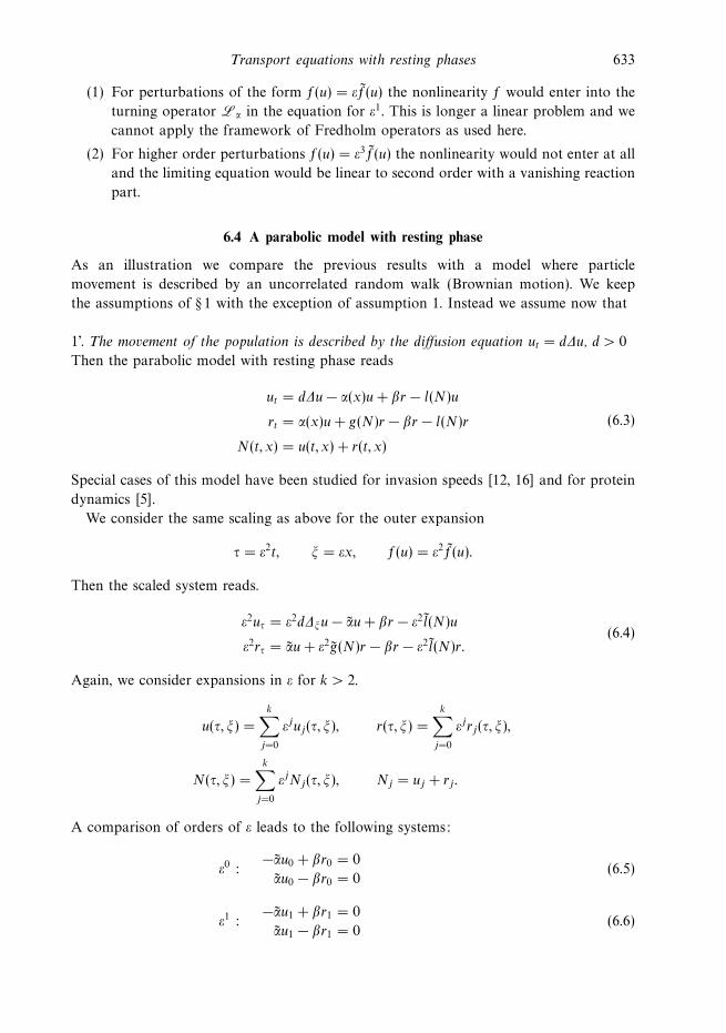
6.4 A parabolic model with resting phase
As an illustration we compare the previous results with a model where particle
movement is described by an uncorrelated random walk (Brownian motion). We keep
the assumptions of § 1 with the exception of assumption 1. Instead we assume now that
1’. The movement of the population is described by the diffusion equation ut = d∆u, d > 0
Then the parabolic model with resting phase reads
ut = d∆u− α(x)u+ βr − l(N)u
rt = α(x)u+ g(N)r − βr − l(N)r
N(t, x) = u(t, x) + r(t, x)
(6.3)
Special cases of this model have been studied for invasion speeds [12, 16] and for protein
dynamics [5].
We consider the same scaling as above for the outer expansion
τ = ε2t, ξ = εx, f(u) = ε2f(u).
Then the scaled system reads.
ε2uτ = ε2d∆ξu− αu+ βr − ε2 l(N)u
ε2rτ = αu+ ε2g(N)r − βr − ε2 l(N)r.(6.4)
Again, we consider expansions in ε for k > 2.
u(τ, ξ) =
k∑j=0
εjuj(τ, ξ), r(τ, ξ) =
k∑j=0
εjrj(τ, ξ),
N(τ, ξ) =
k∑j=0
εjNj(τ, ξ), Nj = uj + rj .
A comparison of orders of ε leads to the following systems:
ε0 :−αu0 + βr0 = 0
αu0 − βr0 = 0(6.5)
ε1 :−αu1 + βr1 = 0
αu1 − βr1 = 0(6.6)

634 T. Hillen
ε2 :u0,τ = d∆u0 − l(N0)u0 − αu2 + βr2r0,τ = αu2 − βr2 + g(N0)r0 − l(N0)r0
(6.7)
From (6.5), it follows that r0 = αβu0, hence N0 = α+ β
βu0. We solve the second equation of
(6.7) for −αu2 + βr2 and use this in the first equation of (6.7) to obtain a single equation
for N0:
N0,τ = d∆
(β
α+ βN0
)+
α
α+ βg(N0)N0 − l(N0)N0,
which can be written in the form:
N0,τ = ∇(
βd
α+ β∇N0 − βd
(α+ β)2∇α N0
)+
α
α+ βg(N0)N0 − l(N0)N0. (6.8)
This equation shows exactly the same scaling in α and β as (3.14) and (3.15). The
reproduction rate is scaled by the mean proportion of the population which is at rest; the
motility is scaled by the mean proportion which is moving; and we obtain a drift toward
high values of α(x).
Remark 6.3 The entire scaling analysis also works for death rates which are different in
moving and resting stages, lp and lr , respectively. It is straightforward to show that the
corresponding term in the diffusion limit is the convex combination:
α
α+ βlr +
β
α+ βlp.
7 Conclusion
In this paper we consider continuum transport models for populations based on individual
movement patterns. The model studied here consists of three major processes: (i) a
correlated random walk, which is described by a transport equation; (ii) kinetics for the
transition from moving to resting, and vice versa; and (iii) kinetics for birth and death.
The resulting model (1.2), (1.3) consists of a nonlinear transport equation coupled with
an ODE.
As listed in the introduction, many applications of this model are discussed in the
literature. These include stream ecosystems, endangered species in fragmented habitats,
homeranges, invasion of new species, hunting territories, prey-taxis, bias toward better
environments, and protein movement in a cell nucleus.
Here we study (1.2), (1.3) from a mathematical point of view and we apply the theory for
the parabolic limit of transport equations which was developed in Hillen & Othmer [13].
In this paper we show:
• Local and global existence of solutions and positivity using standard semigroup argu-
ments.
• On a macroscopic length scale ξ = εx and on a slow time scale τ = ε2t the system is well
described by the outer solution, which satisfies a reaction-advection-diffusion equation
(3.14).

Transport equations with resting phases 635
• The limit equation shows interesting scaling in the relevant parameters. For non constant
α(x) there appears a drift-term toward favorable environments. The diffusion coefficient
is scaled by the mean fraction of moving particles, whereas the birth term is scaled by
the mean fraction of resting particles.
• For homogeneous environments the outer solution approximates the solution of the
transport system (1.2), (1.3) to second order in ε.
• The inner solution is driven by the initial conditions and it ‘lives’ on a fast time scale t
and the macroscopic length scale ξ. The inner solution converges to a distribution which
is homogeneous in v, which matches to the initial conditions of the outer solution.
• We consider special cases for perturbed homogeneous initial conditions, for a large
fraction of particles in resting or moving states, and we study a diffusion based model
which includes resting-moving dynamics.
In further studies we shall apply the theory to the examples mentioned earlier, in
particular to bat-territories and to prey-taxis.
Moreover, it would be interesting to see if oriented movement is beneficial for a
population, as done by Cosner et al. [8, 2] for the parabolic limit model.
We expect that the theory, as used here, can be readily extended to include different
death rates for moving and resting compartments, or to include a spatially dependent
starting rate β(x). It is more of a challenge, however, to include inhomogeneities which
show jumps in the quality of the habitat, i.e. jumps in α(x). In (A3) we assumed that α(x)
is continuous, which excludes jumps. The functional analysis, which underlies the studies,
has to be re-investigated for that case.
References
[1] Alt, W. (1981) Singular perturbation of differential integral equations describing biased
random walks. J. Reine Angew. Math. 322, 15–41.
[2] Belgacem, F. & Cosner, C. (1995) The effects of dispersal along environmental gradients on
the dynamics of populations in heterogeneous environment. Canadian Appl. Math. Quart. 3,
379–397.
[3] Briscoe, B., Lewis, M. & Parisch, S. (2002) Home range formation in wolves due to scent
marking. Bull. Math. Biol. 64, 261–284.
[4] Britton, N. F. (1986) Reaction–Diffusion Equations and Their Applications to Biology.
Academic Press.
[5] Carrero, G., McDonald, D., Crawford, E., de Vries, G. & Hendzel, M. (2003) Using
FRAP and mathematical modeling to determine the in vivo kinetics of nuclear proteins.
Methods, 29, 14–28.
[6] Carroll, J. & Lamberson, R. (1993) The owl’s odyssey. A continuous model for the dispersal
of territorial species. SIAM J. Appl. Math. 53, 205–218.
[7] Chueh, K. N., Conley, C. C. & Smoller, J. A. (1977) Positively invariant regions for systems
of nonlinear diffusion equations. Indiana Univ. Math. J. 26, 373–392.
[8] Cosner, C. & Lou, Y. (2003) Does movement toward better environments always benefit a
population? J. Math. Anal. Appl. 277, 489–503.
[9] Dautray, R. & Lions, J.-L. (1993) Mathematical Analysis and Numerical Methods for Science
and Technology, VI. Springer-Verlag.
[10] Dickinson, R. (2000) A generalized transport model for biased cell migration in an anisotropic
environment. J. Math. Biol. 40, 97–135.

636 T. Hillen
[11] Hadeler, K. P. (1998) Reaction transport systems. In: Capasso, V. and Diekmann, O. (editors),
Mathematics Inspired by Biology: CIME Letures 1997, pp. 95–150. Springer-Verlag.
[12] Hadeler, K. P. & Lewis, M. (2003) Spatial dynamics of the diffusive logistic equation with
sedentary compartment. Canad. Appl. Math. Quart. (to appear).
[13] Hillen, T. & Othmer, H. G. (2000) The diffusion limit of transport equations derived from
velocity jump processes. SIAM J. Appl. Math. 61(3), 751–775.
[14] Kareiva, P. & Odell, G. (1987) Swarms of predators exhibit ’prey-taxis’ if individual predators
use area-restricted search. Am. Naturalist, 130(2), 233–270.
[15] Ladyzhenskaja, O. A., Solonnikov, V. A. & Ural’ceva, N. N. (1968) Linear and Quasilinear
Equations of Parabolic Type. AMS.
[16] Lewis, M. A. & Schmitz, G. (1996) Biological invasion of an organism with separate mobile
and stationary states: Modeling and analysis. Forma, 11, 1–25.
[17] Muller, K. (1954) Investigation on the organic drift in north Swedish streams. Report of the
Inst. Fresh Water Reserach, Drottingholm, 34, pp. 133–148.
[18] Murray, J. D. (1989) Mathematical Biology. Springer-Verlag.
[19] Othmer, H. G., Dunbar, S. R. & Alt, W. (1988) Models of dispersal in biological systems.
J. Math. Biol. 26, 263–298.
[20] Othmer, H. G. & Hillen, T. (2002) The diffusion limit of transport equations (ii): Chemotaxis
equations. SIAM J. Appl. Math. 62(4), 1122–1250.
[21] Pachepsky, E., Lewis, M. & Lutscher, F. (2003) Persistence, spread and the drift paradox.
Theor. Pop. Biol. (submitted)
[22] Pazy, A. (1983) Semigroups of Linear Operators and Applications to Partial Differential Equa-
tions. Springer-Verlag.
[23] Stroock, D. W. (1974) Some stochastic processes which arise from a model of the motion of
a bacterium. Probab. Theory Rel. Fields, 28, 305–315.
[24] Taylor, M. E. (1996) Partial Differential Equations III. Springer-Verlag.