Embed Size (px)
Citation preview
PEE 372: Transportation and Storage Instructor : Dr. Salem S. Al-Marri
Office: Building No. 6 Office No. 149
Petroleum Engineering Technology
College of Technological Studies (CTS)
Public Authority for Applied Education and Training (PAAET)
Email: [email protected]
Course Contents
• Fluid Properties
• ----
• ----
• ----
• ----
• ----
• ----
Course Grade System
Lecture Grade: 100%
The lecture grades will be divided as follows:
Attendance 10%
H.W. & Quizzes 10%
Mid-Terms 40%
Final Exam 40%
Total 100%
Lecture: Section# 1: Thursday 3-5 PM
1
Transportation and Storage
Lecture # 1
Introduction to
Fluid Properties
2
3
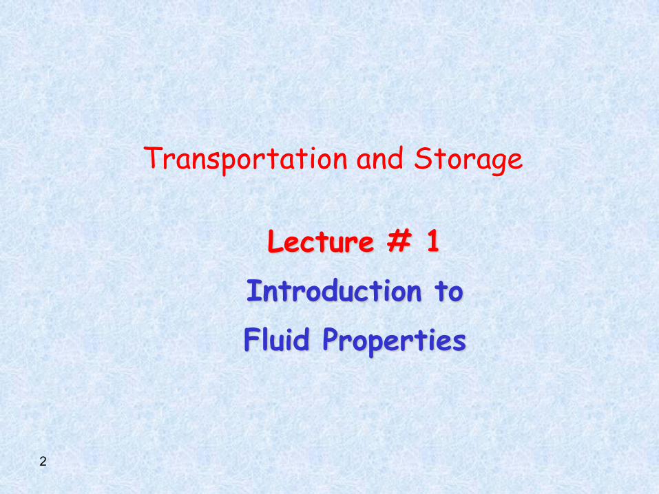
Classification of Reservoir Fluid Chemical Properties
PNA and combinations (Paraffinic-Naphthenic-Aromatics)
Resin and asphalthene content
Physical Properties
Phase density (liquid, gas, solid)
Compressibility
Viscosity
Formation volume factor
Gas Oil Ratio
Surface tension
Heat capacity
Thermal conductivity
Pour and Cloud points
4
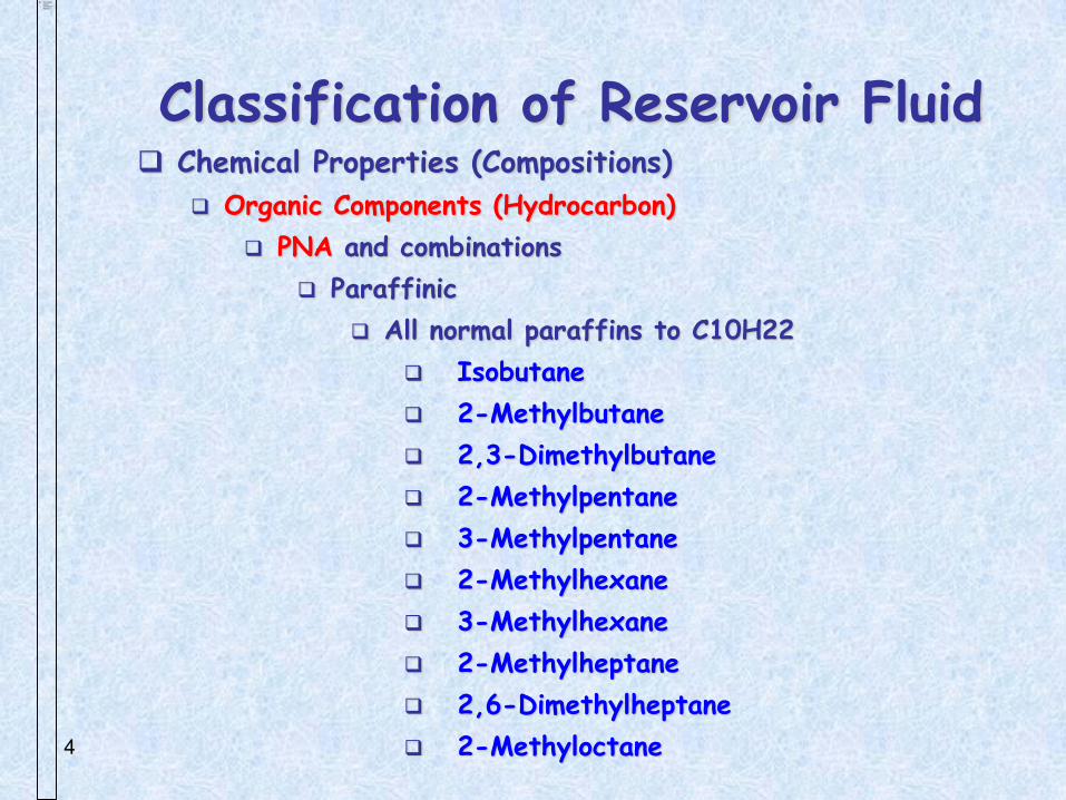
Classification of Reservoir Fluid Chemical Properties (Compositions)
Organic Components (Hydrocarbon)
PNA and combinations
Paraffinic
All normal paraffins to C10H22
Isobutane
2-Methylbutane
2,3-Dimethylbutane
2-Methylpentane
3-Methylpentane
2-Methylhexane
3-Methylhexane
2-Methylheptane
2,6-Dimethylheptane
2-Methyloctane
5
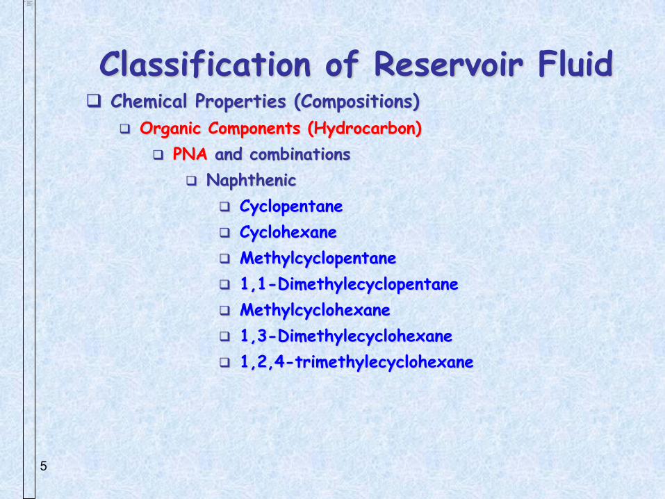
Classification of Reservoir Fluid Chemical Properties (Compositions)
Organic Components (Hydrocarbon)
PNA and combinations
Naphthenic
Cyclopentane
Cyclohexane
Methylcyclopentane
1,1-Dimethylecyclopentane
Methylcyclohexane
1,3-Dimethylecyclohexane
1,2,4-trimethylecyclohexane
6
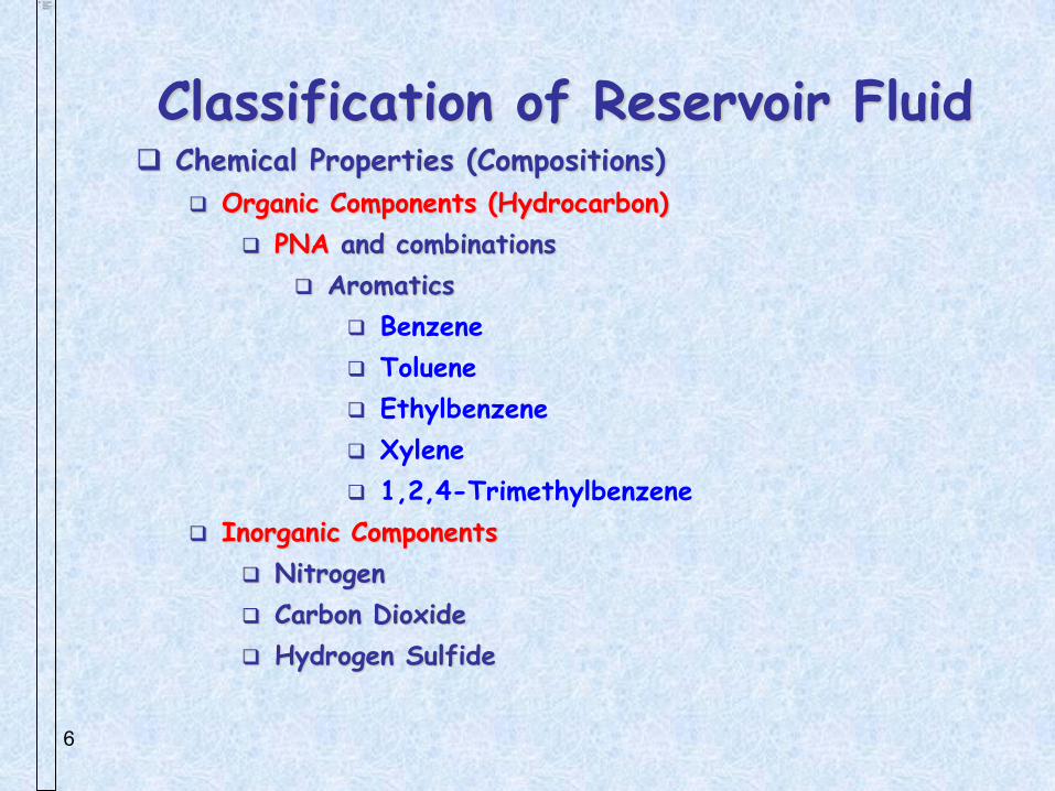
Classification of Reservoir Fluid Chemical Properties (Compositions)
Organic Components (Hydrocarbon)
PNA and combinations
Aromatics
Benzene
Toluene
Ethylbenzene
Xylene
1,2,4-Trimethylbenzene
Inorganic Components
Nitrogen
Carbon Dioxide
Hydrogen Sulfide
7
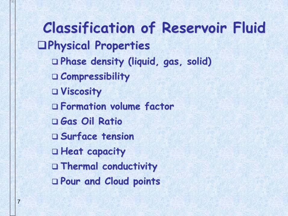
Classification of Reservoir Fluid Physical Properties
Phase density (liquid, gas, solid)
Compressibility
Viscosity
Formation volume factor
Gas Oil Ratio
Surface tension
Heat capacity
Thermal conductivity
Pour and Cloud points
8
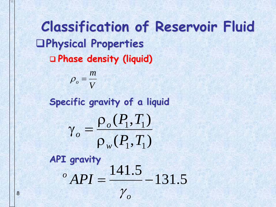
Classification of Reservoir Fluid Physical Properties
Phase density (liquid)
Specific gravity of a liquid
API gravity
o
m
V
),(
),(
11
11
TP
TP
w
oo
141.5131.5o
o
API
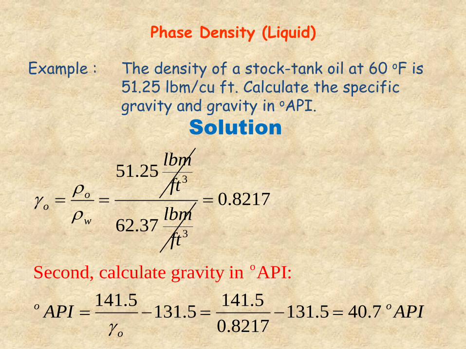
Phase Density (Liquid)
Example : The density of a stock-tank oil at 60 oF is 51.25 lbm/cu ft. Calculate the specific gravity and gravity in oAPI.
Solution
351.25
oo
w
lbm
ft
362.37
lbm
ft
oSecond, calculate gravity in A
0.8217
141.5 141.5131.5 131.5 40.7
0.8
PI:
217
o o
o
API API
10
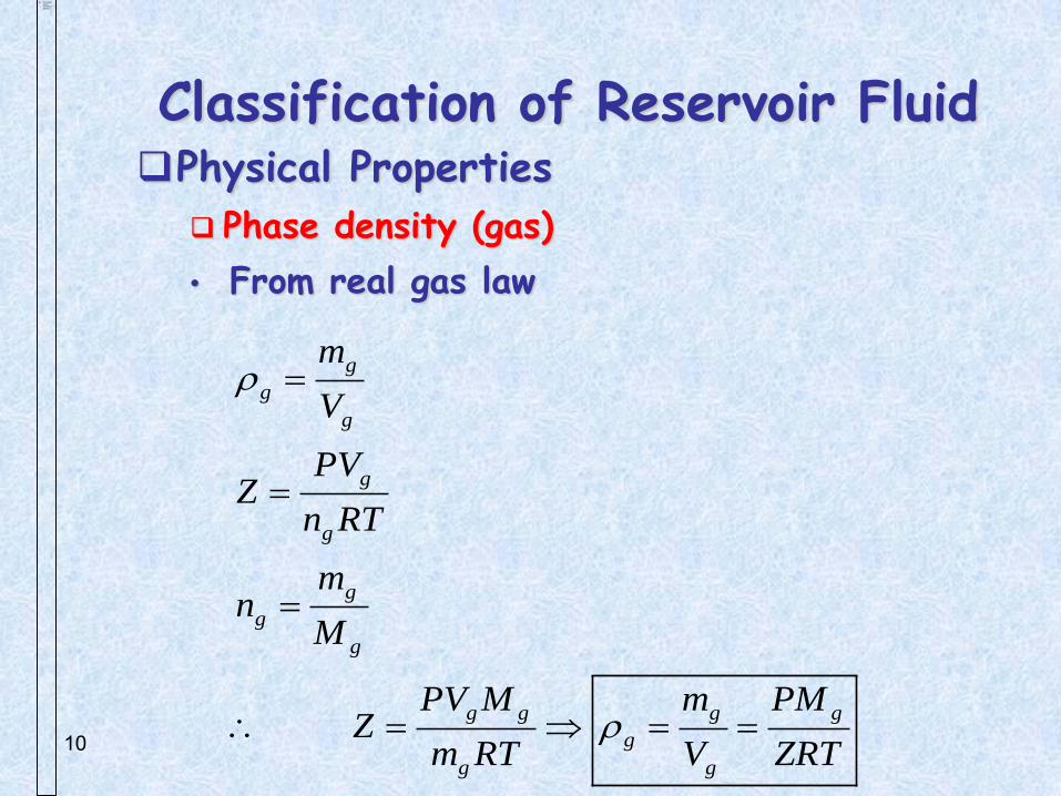
Classification of Reservoir Fluid Physical Properties
Phase density (gas)
• From real gas law
g
g
g
g
g
g
g
g
g g g g
g
g g
m
V
PVZ
n RT
mn
M
PV M m PMZ
m RT V ZRT
11
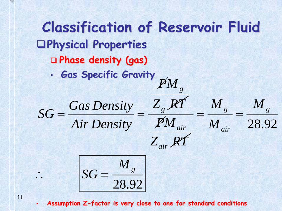
Classification of Reservoir Fluid Physical Properties
Phase density (gas)
• Gas Specific Gravity
• Assumption Z-factor is very close to one for standard conditions
g
g
PM
Z RTGas DensitySG
Air Density
air
air
PM
Z RT
28.92
28.92
g g
air
g
M M
M
MSG
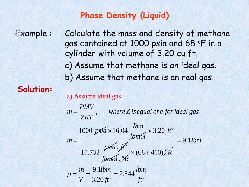
Phase Density (Liquid)
Example : Calculate the mass and density of methane gas contained at 1000 psia and 68 oF in a cylinder with volume of 3.20 cu ft.
a) Assume that methane is an ideal gas.
b) Assume that methane is an real gas.
Solution:
a) Assume ideal g
,
100
s
0
a
PMVm where Z is equal one for ideal gas
ZRT
psia
m
16.04lbm
lbmol 33.20 ft
10.732psia 3. ft
lbmol . oR(68 460) oR
3 3
9.1
9.12.844
3.20
lbm
m lbm lbm
V ft ft
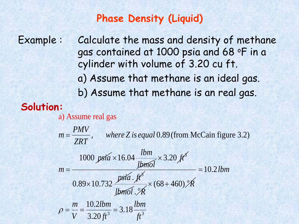
Phase Density (Liquid)
Example : Calculate the mass and density of methane gas contained at 1000 psia and 68 oF in a cylinder with volume of 3.20 cu ft.
a) Assume that methane is an ideal gas.
b) Assume that methane is an real gas.
Solution:
, 0.89(from McCain fig
a
ure 3
) Assume real gas
.2)
1000
PMVm where Z is equal
ZRT
psia
m
16.04lbm
lbmol 33.20 ft
0.89 10.732psia
3. ft
lbmol . oR(68 460) oR
3 3
10.2
10.23.18
3.20
lbm
m lbm lbm
V ft ft
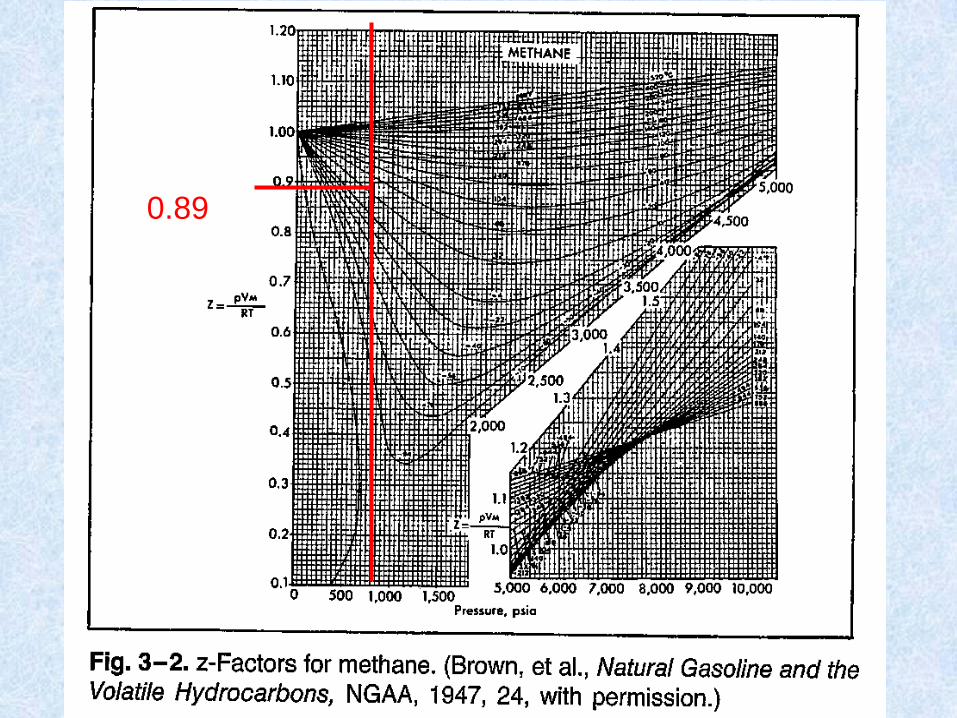
0.89
15
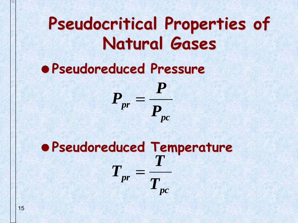
Pseudocritical Properties of Natural Gases
Pseudoreduced Pressure
Pseudoreduced Temperature
pc
prP
PP
pc
prT
TT
16
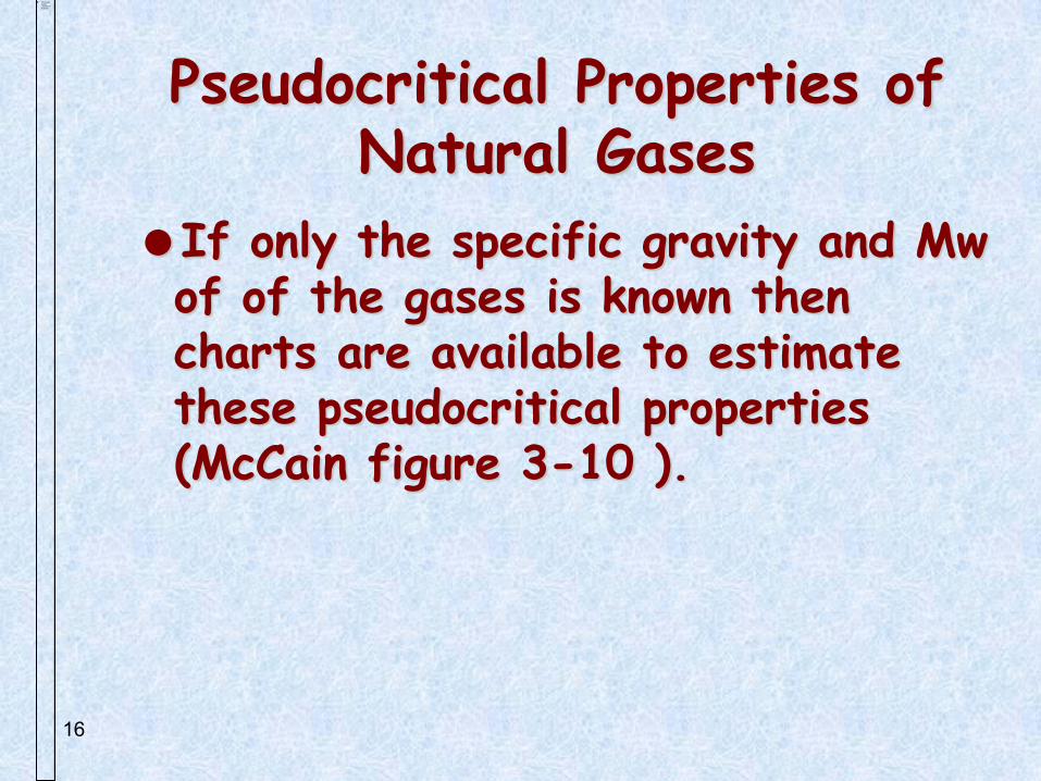
Pseudocritical Properties of Natural Gases
If only the specific gravity and Mw of of the gases is known then charts are available to estimate these pseudocritical properties (McCain figure 3-10 ).

17
Pseudocritical Properties of Natural Gases
Naturally the degree of accuracy is reduced substantially. We well see methods when compositional information is available, in this case:
cii
N
i
pc PyPc
1
cii
N
i
pc TyTc
1
18
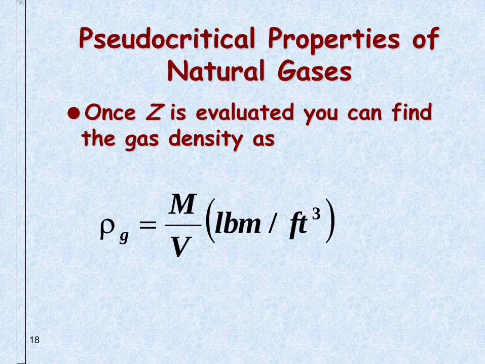
Pseudocritical Properties of Natural Gases
Once Z is evaluated you can find the gas density as
3/ ftlbm
V
Mg
19
Z-factor
chart for
low
reduced
pressures
20
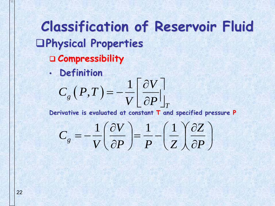
Classification of Reservoir Fluid Physical Properties
Compressibility
• Definition
Derivative is evaluated at constant T=TA and specified pressure P=PA
1
,
A
g A A
T
VC P T
V P
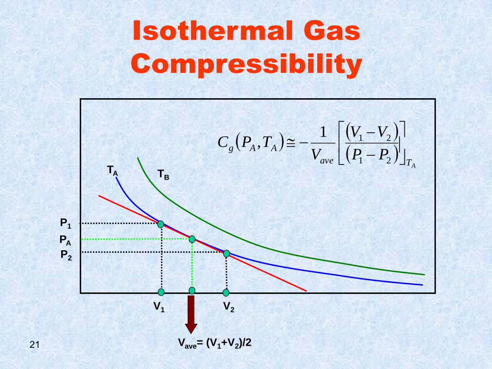
Isothermal Gas
Compressibility
P1
V2 V1
TB
P2
Vave= (V1+V2)/2
ATave
AAgPP
VV
VTPC
21
211,
TA
PA
21
22
Classification of Reservoir Fluid Physical Properties
Compressibility
• Definition
Derivative is evaluated at constant T and specified pressure P
1
,g
T
VC P T
V P
P
Z
ZPP
V
VCg
111
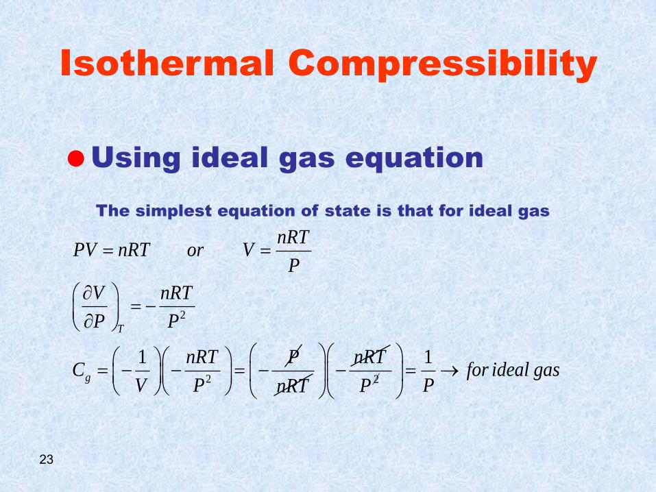
Isothermal Compressibility
Using ideal gas equation
The simplest equation of state is that for ideal gas
23
2
2
1
T
g
nRTPV nRT or V
P
V nRT
P P
nRT PC
V P
nRT
nRT
2
1for ideal gas
PP
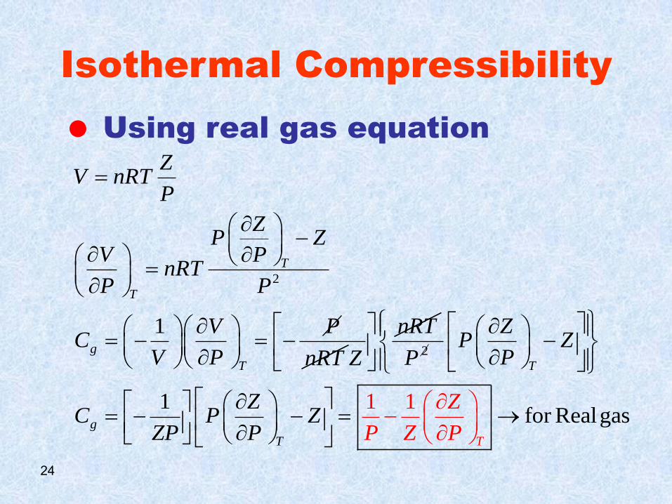
Isothermal Compressibility
Using real gas equation
24
2
1
T
T
g
T
ZV nRT
P
ZP Z
V PnRT
P P
V PC
V P nRT
nRT
Z
2
1for Realgas
1 1
T
g
T T
ZP Z
PP
ZC P
Z
Z PZ
P ZP P
Isothermal Compressibility (Cg) of an Ideal Gas
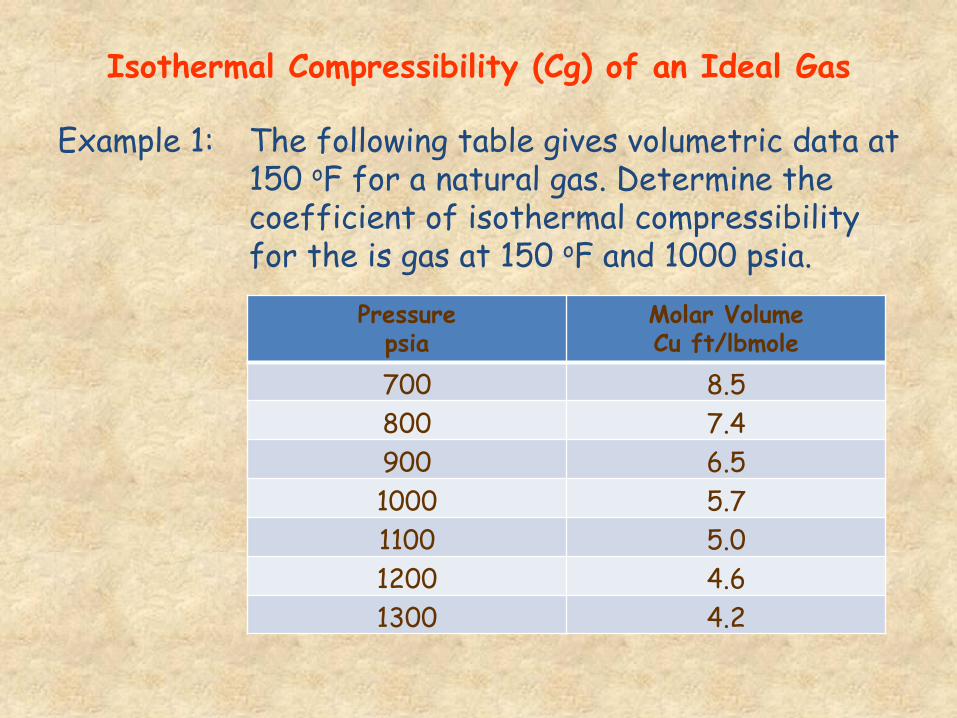
Example 1: The following table gives volumetric data at 150 oF for a natural gas. Determine the coefficient of isothermal compressibility for the is gas at 150 oF and 1000 psia.
Pressure psia
Molar Volume Cu ft/lbmole
700 8.5
800 7.4
900 6.5
1000 5.7
1100 5.0
1200 4.6
1300 4.2
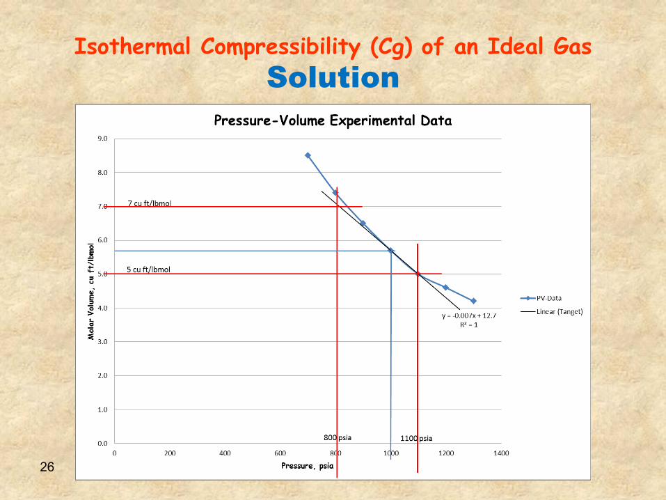
Isothermal Compressibility (Cg) of an Ideal Gas
Solution
26
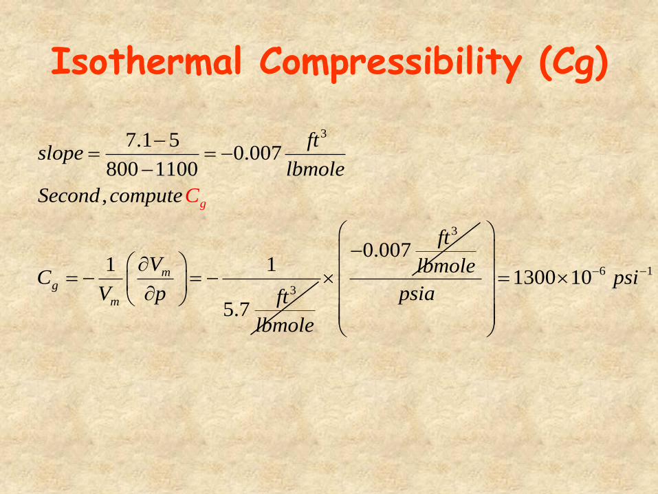
Isothermal Compressibility (Cg)
3
3
7.1 50.007
800 1100
,
1 1
5.7m
g
mg
ftslope
lbmole
Second compute
VC
V p ft
lbmole
C
3
0.007ft
lbmole
6 11300 10 psipsia
Isothermal Compressibility (Cg) of an Real Gas
Example 2: Compute the coefficient of isothermal compressibility of ethane at 1000 psia and 212 oF.
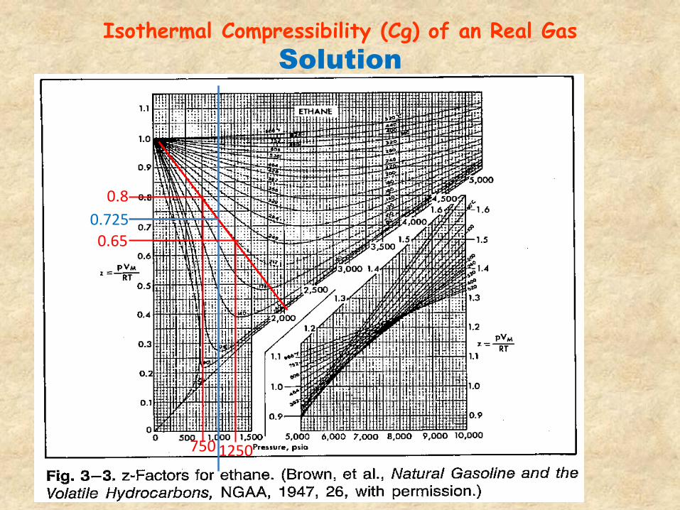
Isothermal Compressibility (Cg) of an Real Gas
Solution
0.8
0.65
1250 750
0.725
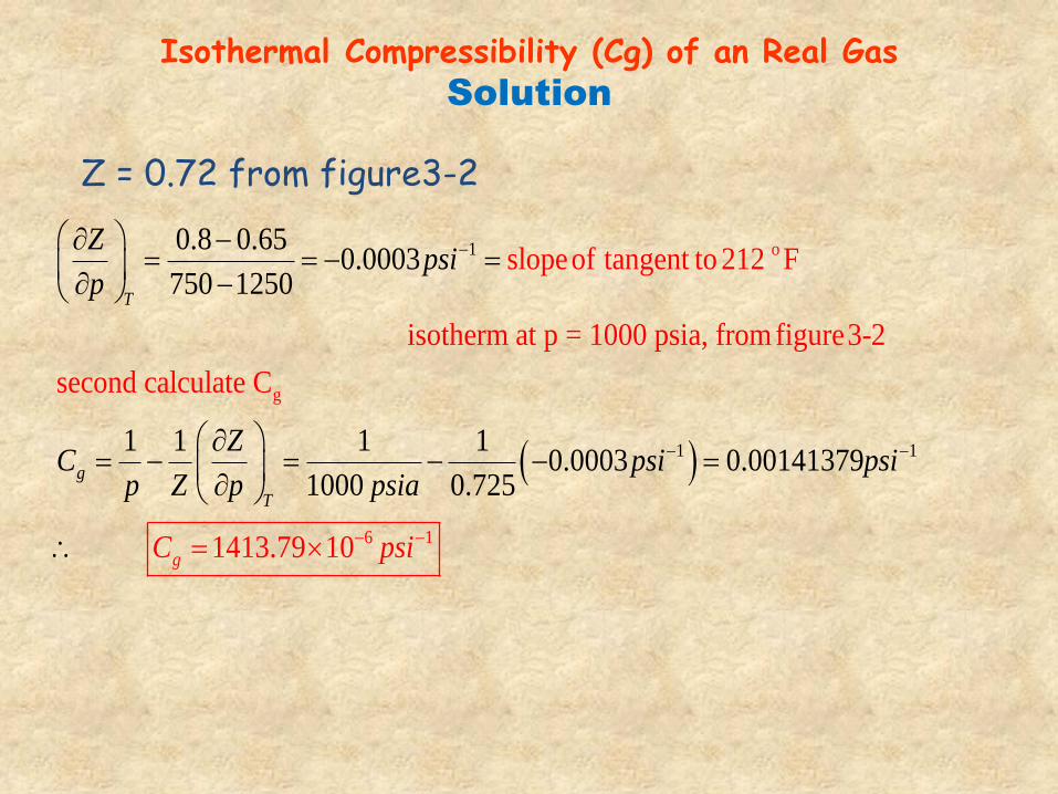
Isothermal Compressibility (Cg) of an Real Gas Solution
Z = 0.72 from figure3-2
1
1 1
o
g
slopeof tangent to 212 F
isotherm at p = 1000 psia, from figure3-2
second calculate C
1413.79 1
0.8 0.650.0003
750 1250
1 1 1 10.0003 0.00141379
1000 0.
0
725
T
g
T
g
Zpsi
p
ZC psi psi
p Z p psia
C
6 1psi
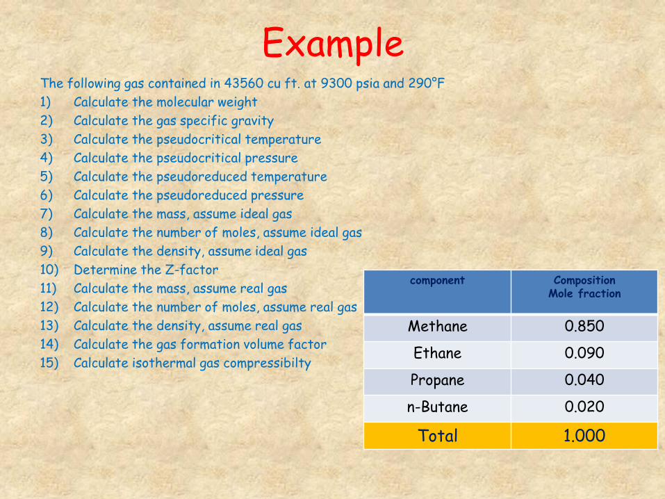
Example The following gas contained in 43560 cu ft. at 9300 psia and 290°F
1) Calculate the molecular weight
2) Calculate the gas specific gravity
3) Calculate the pseudocritical temperature
4) Calculate the pseudocritical pressure
5) Calculate the pseudoreduced temperature
6) Calculate the pseudoreduced pressure
7) Calculate the mass, assume ideal gas
8) Calculate the number of moles, assume ideal gas
9) Calculate the density, assume ideal gas
10) Determine the Z-factor
11) Calculate the mass, assume real gas
12) Calculate the number of moles, assume real gas
13) Calculate the density, assume real gas
14) Calculate the gas formation volume factor
15) Calculate isothermal gas compressibilty
component Composition Mole fraction
Methane 0.850
Ethane 0.090
Propane 0.040
n-Butane 0.020
Total 1.000
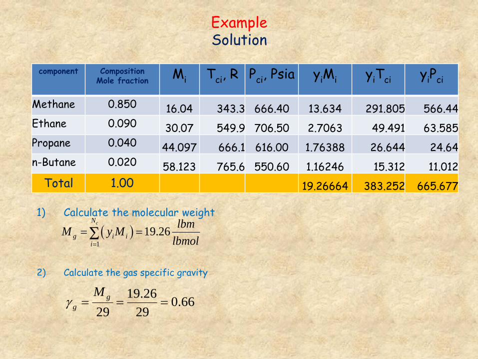
Example Solution
component Composition Mole fraction
Mi Tci, R Pci, Psia yiMi yiTci yiPci
Methane 0.850 16.04 343.3 666.40 13.634 291.805 566.44
Ethane 0.090 30.07 549.9 706.50 2.7063 49.491 63.585
Propane 0.040 44.097 666.1 616.00 1.76388 26.644 24.64
n-Butane 0.020 58.123 765.6 550.60 1.16246 15.312 11.012
Total 1.00 19.26664 383.252 665.677
1) Calculate the molecular weight
2) Calculate the gas specific gravity
1
19.26cN
g i ii
lbmM y M
lbmol
19.260.66
29 29
g
g
M
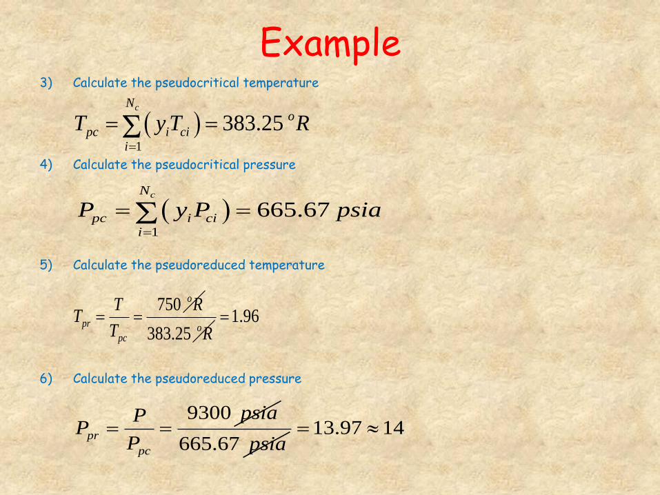
Example 3) Calculate the pseudocritical temperature
4) Calculate the pseudocritical pressure
5) Calculate the pseudoreduced temperature
6) Calculate the pseudoreduced pressure
1
383.25cN
o
pc i cii
T y T R
1
665.67cN
pc i cii
P y P psia
750 o
pr
pc
T RT
T
383.25 oR1.96
9300pr
pc
psiaPP
P
665.67 psia13.97 14
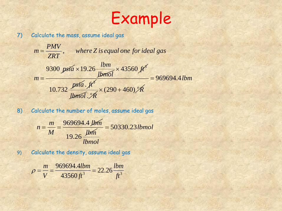
Example 7) Calculate the mass, assume ideal gas
8) Calculate the number of moles, assume ideal gas
9) Calculate the density, assume ideal gas
,
9300
PMVm where Z is equal one for ideal gas
ZRT
psia
m
19.26lbm
lbmol 343560 ft
10.732psia 3. ft
lbmol . oR(290 460) oR
969694.4 lbm
969694.4m lbmn
M
19.26lbm
50330.23lbmol
lbmol
3 3
969694.422.26
43560
m lbm lbm
V ft ft
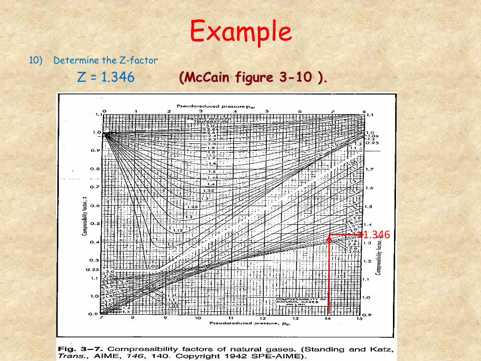
Example 10) Determine the Z-factor
Z = 1.346 (McCain figure 3-10 ).
1.346
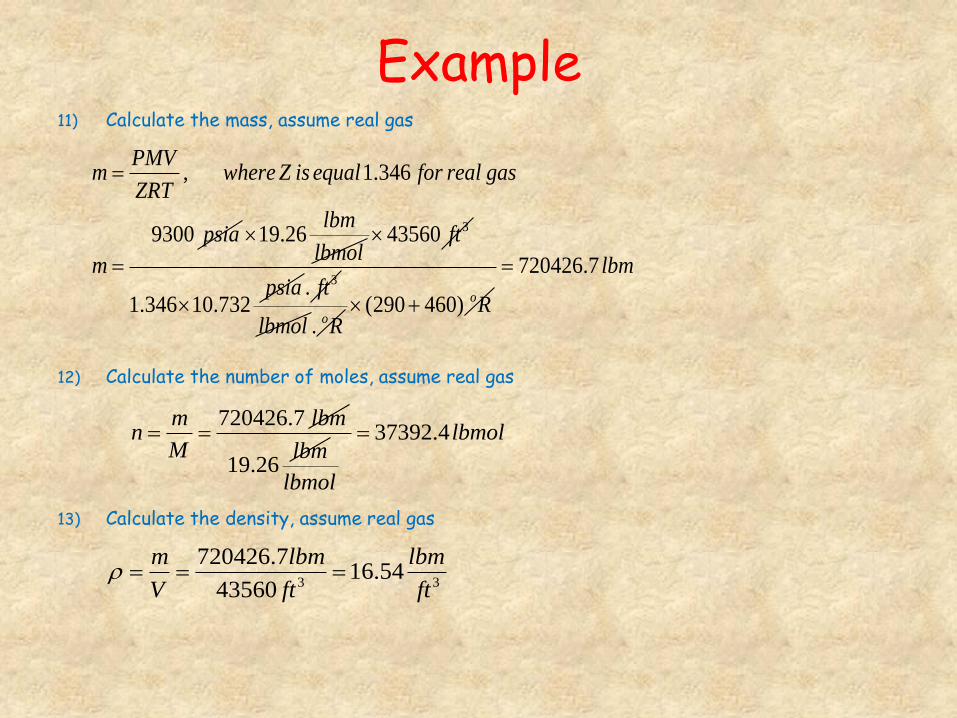
Example 11) Calculate the mass, assume real gas
12) Calculate the number of moles, assume real gas
13) Calculate the density, assume real gas
, 1.346
9300
PMVm where Z is equal for real gas
ZRT
psia
m
19.26lbm
lbmol 343560 ft
1.346 10.732psia
3. ft
lbmol . oR(290 460) oR
720426.7 lbm
720426.7m lbmn
M
19.26lbm
37392.4 lbmol
lbmol
3 3
720426.716.54
43560
m lbm lbm
V ft ft
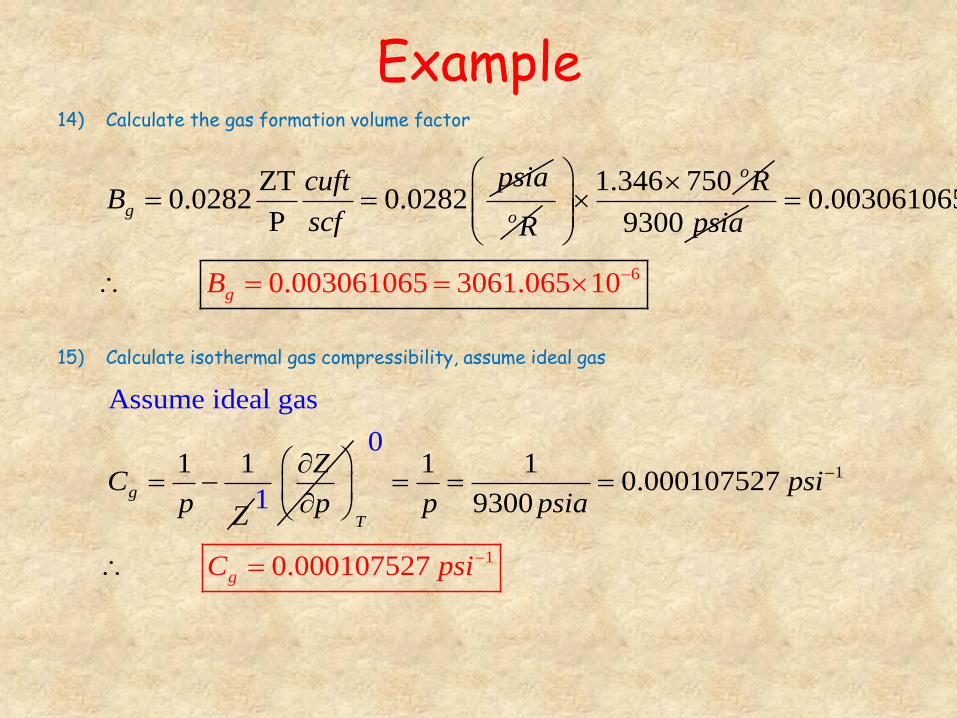
Example 14) Calculate the gas formation volume factor
15) Calculate isothermal gas compressibility, assume ideal gas
ZT0.0282 0.0282
Pg
psiacuftB
scf
oR
1.346 750 oR
9300 psia
60.003061065
0.003061065
3061.065 10gB
Assume ideal gas
1 1gC
p Z
1
Z
p
1
1
1 10.000107527
0.000107
9300
7
0
52
T
gC
p
ps
sip sia
i
p
38
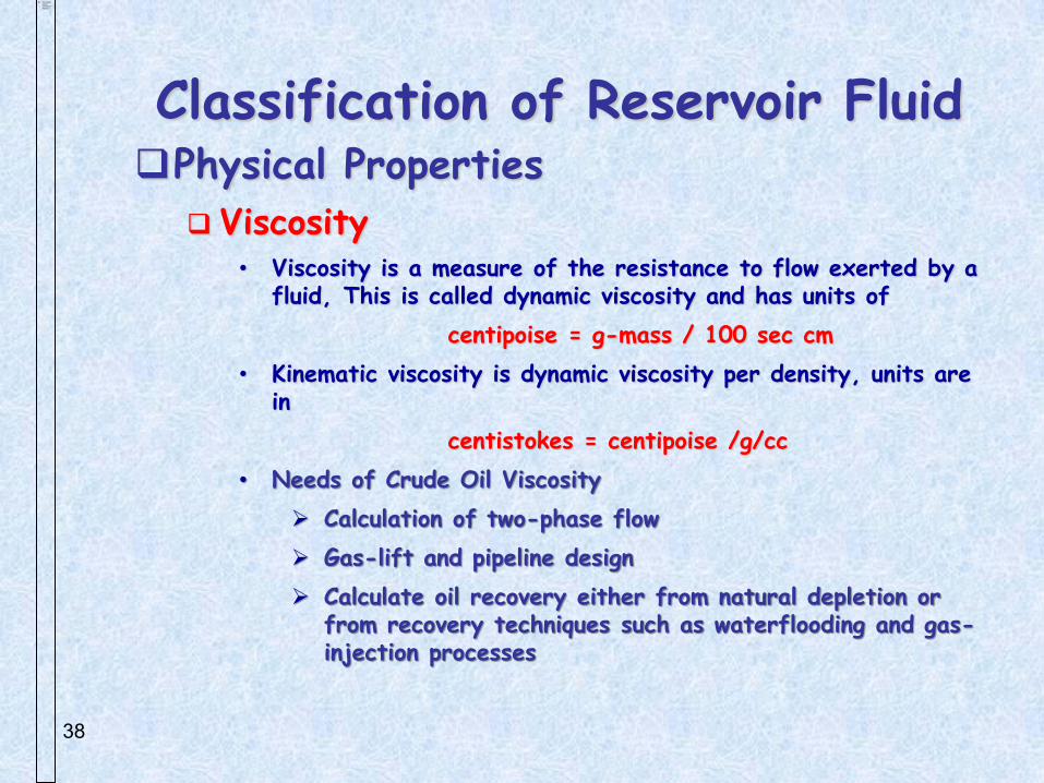
Classification of Reservoir Fluid Physical Properties
Viscosity • Viscosity is a measure of the resistance to flow exerted by a
fluid, This is called dynamic viscosity and has units of
centipoise = g-mass / 100 sec cm
• Kinematic viscosity is dynamic viscosity per density, units are in
centistokes = centipoise /g/cc
• Needs of Crude Oil Viscosity
Calculation of two-phase flow
Gas-lift and pipeline design
Calculate oil recovery either from natural depletion or from recovery techniques such as waterflooding and gas-injection processes
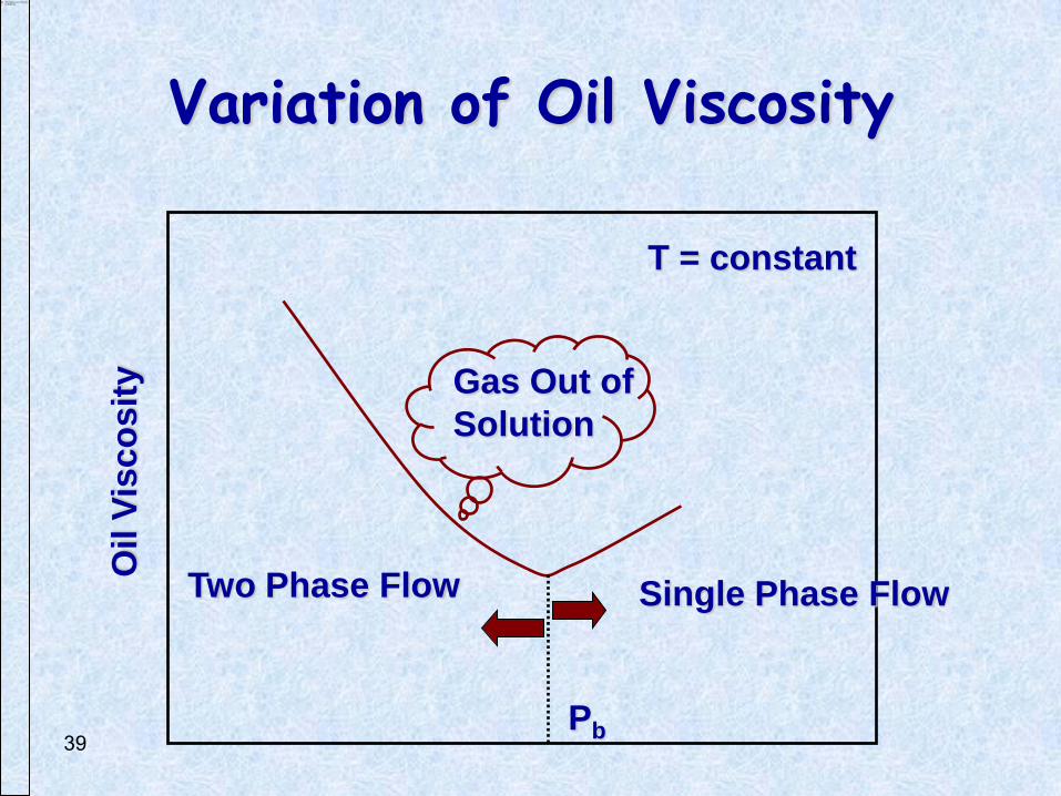
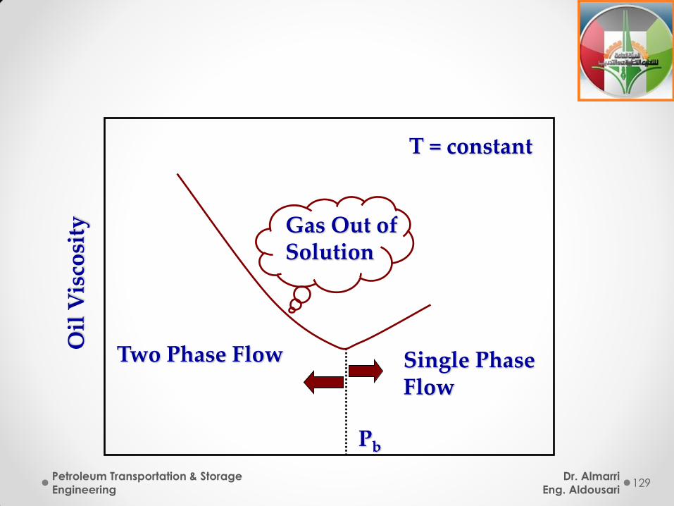
Variation of Oil Viscosity O
il V
isco
sit
y
T = constant
Pb
Single Phase Flow
Two Phase Flow
Gas Out of
Solution
39
40
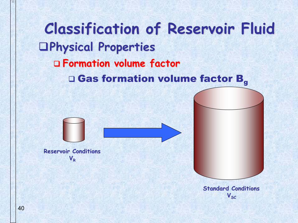
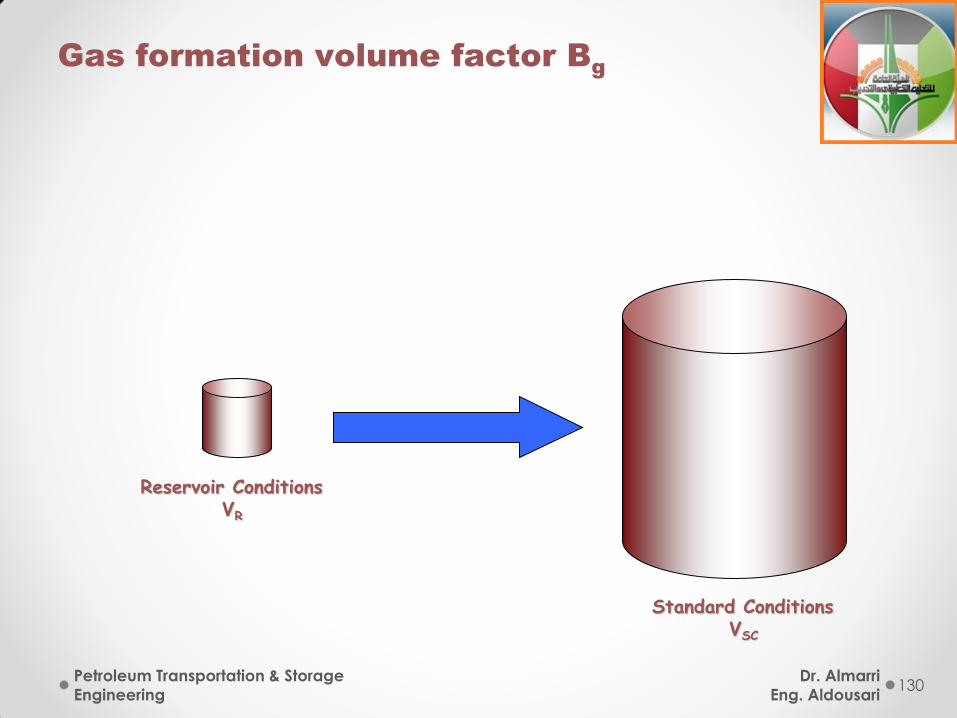
Classification of Reservoir Fluid Physical Properties
Formation volume factor
Gas formation volume factor Bg
Reservoir Conditions VR
Standard Conditions VSC
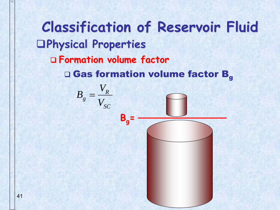
41
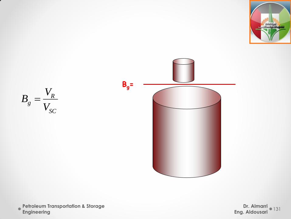
Classification of Reservoir Fluid Physical Properties
Formation volume factor
Gas formation volume factor Bg
Bg=
Rg
SC
VB
V

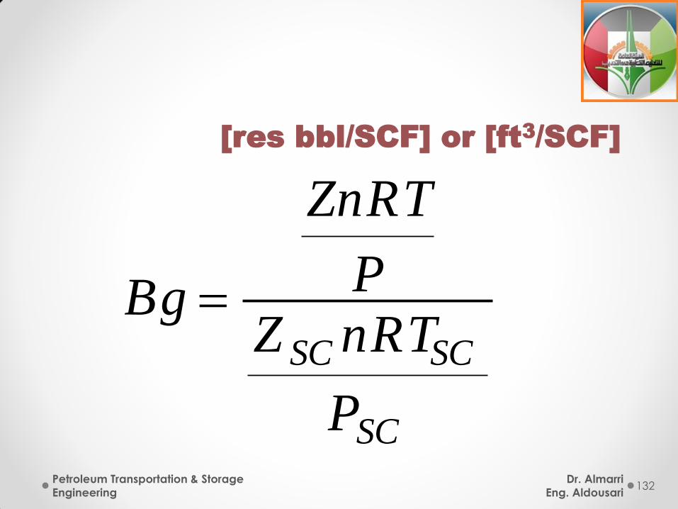
[res bbl/SCF] or [ft3/SCF]
Gas Formation Volume
Factor
SC
SCSC
P
nRTZ
P
ZnRT
Bg
42
Gas Formation Volume
Factor
43
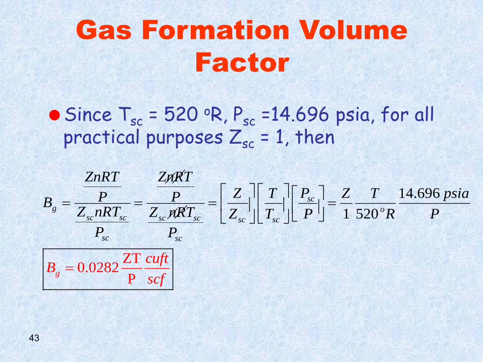
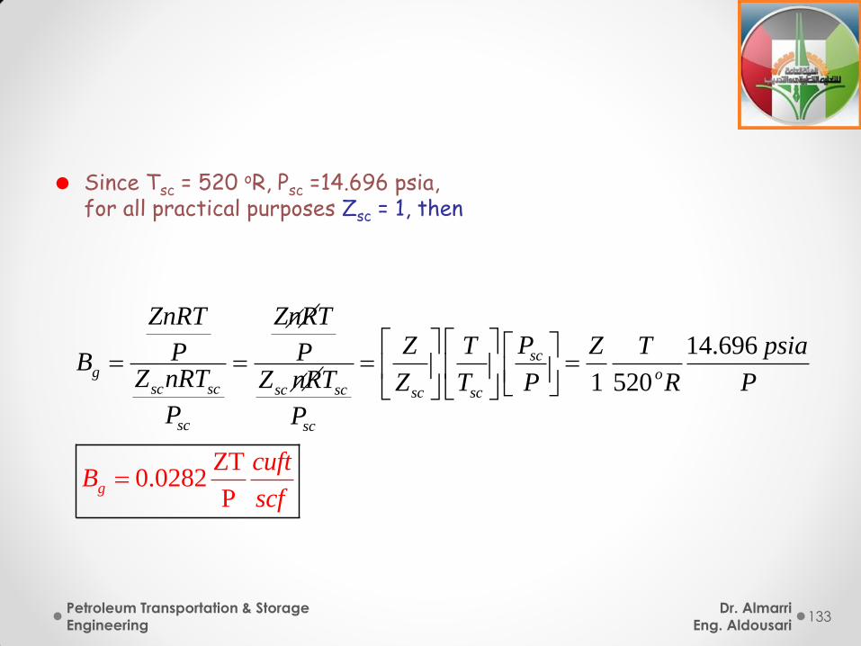
Since Tsc = 520 oR, Psc =14.696 psia, for all practical purposes Zsc = 1, then
14.6
ZT0.02
96
1 520
82P
scg o
sc sc sc sc sc sc
sc c
g
s
ZnRT ZnRTPZ T Z T psiaP PB
Z nRT Z nRT Z T P R P
cuftB
cf
P P
s
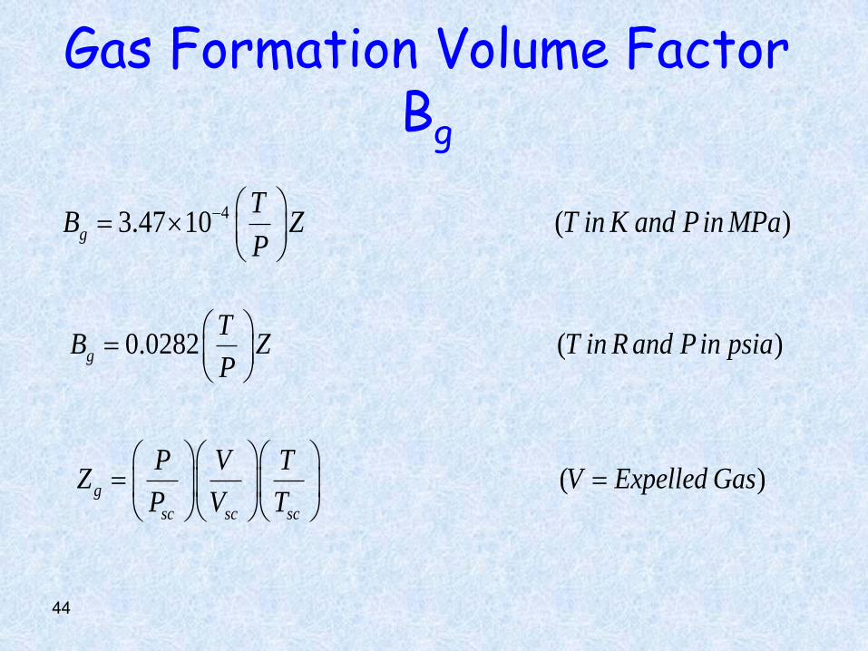
Gas Formation Volume Factor Bg
43.47 10 ( )g
TB Z T in K and Pin MPa
P
0.0282 ( )g
TB Z T in R and Pin psia
P
( )g
sc sc sc
P V TZ V Expelled Gas
P V T
44
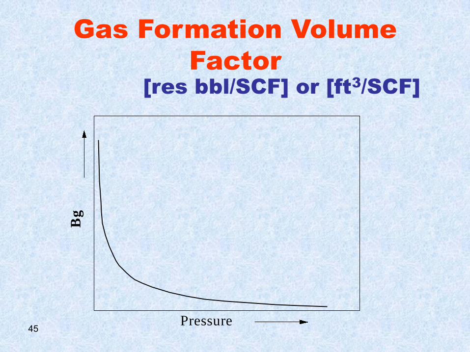
[res bbl/SCF] or [ft3/SCF]
Gas Formation Volume
Factor
Gas Formation Volume Factor
Bg
Pressure45
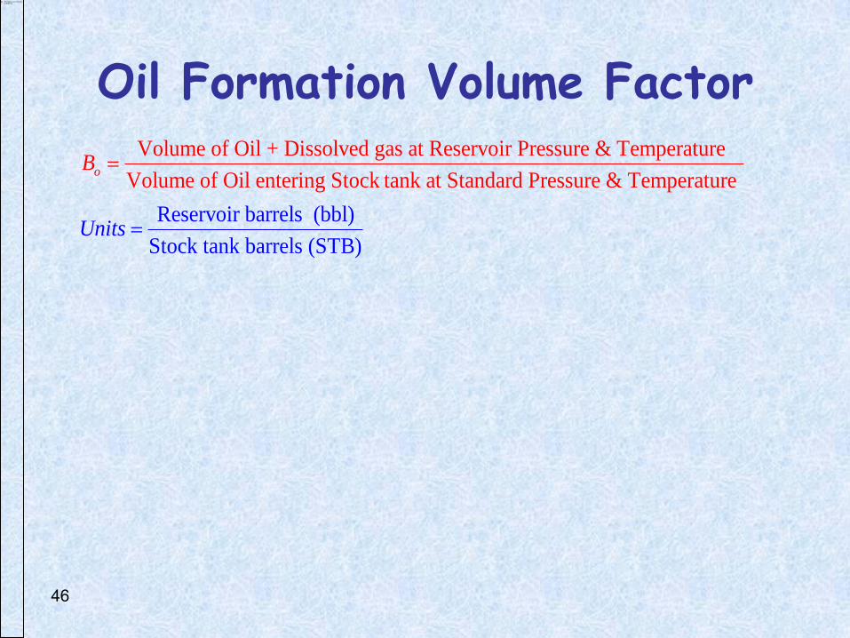
Oil Formation Volume Factor
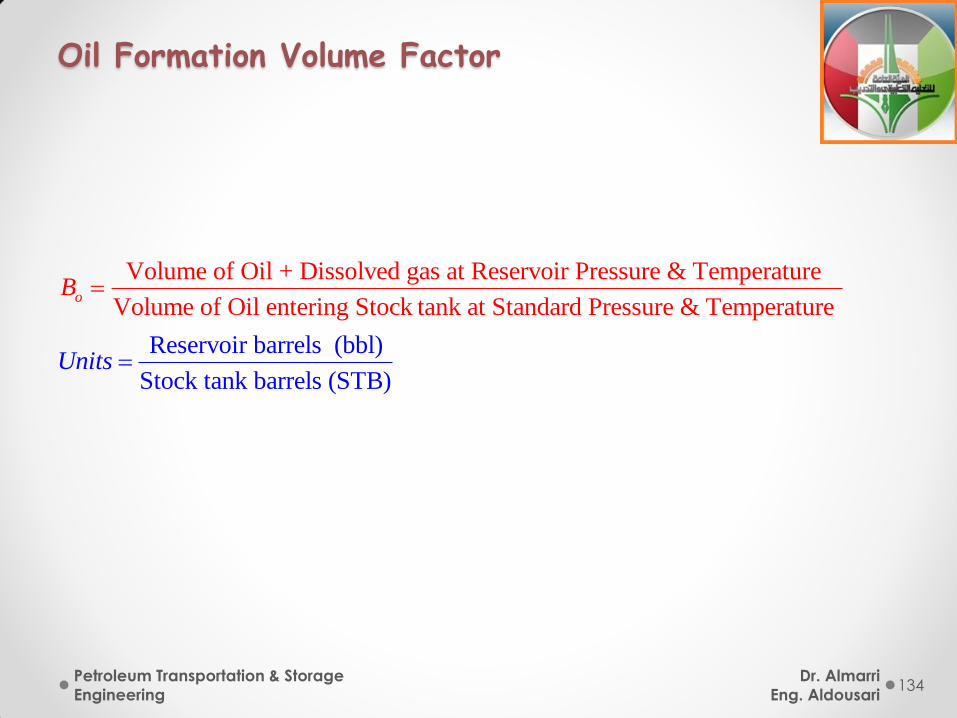
46
Volume of Oil + Dissolved gas at Reservoir Pressure & Temperature
Volume of Oil entering Stoc
Reservoir barrels (bbl)
Stock tank barrels (
k tank at Standard Pressure & Temper
STB)
ature o
Units
B
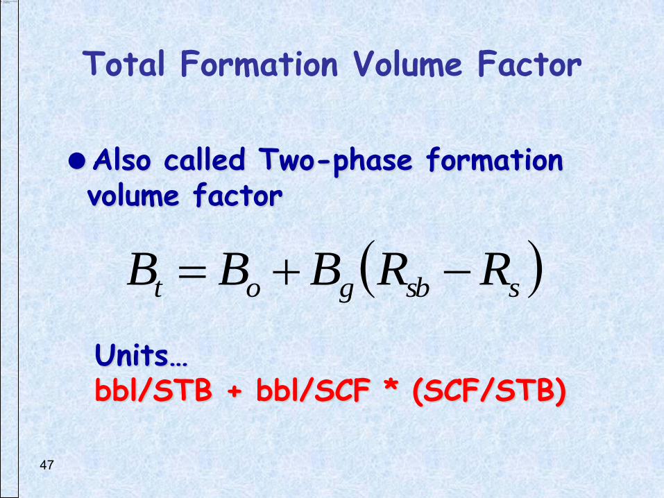
Total Formation Volume Factor
Also called Two-phase formation volume factor
ssbgot RRBBB
Units…
bbl/STB + bbl/SCF * (SCF/STB)
47
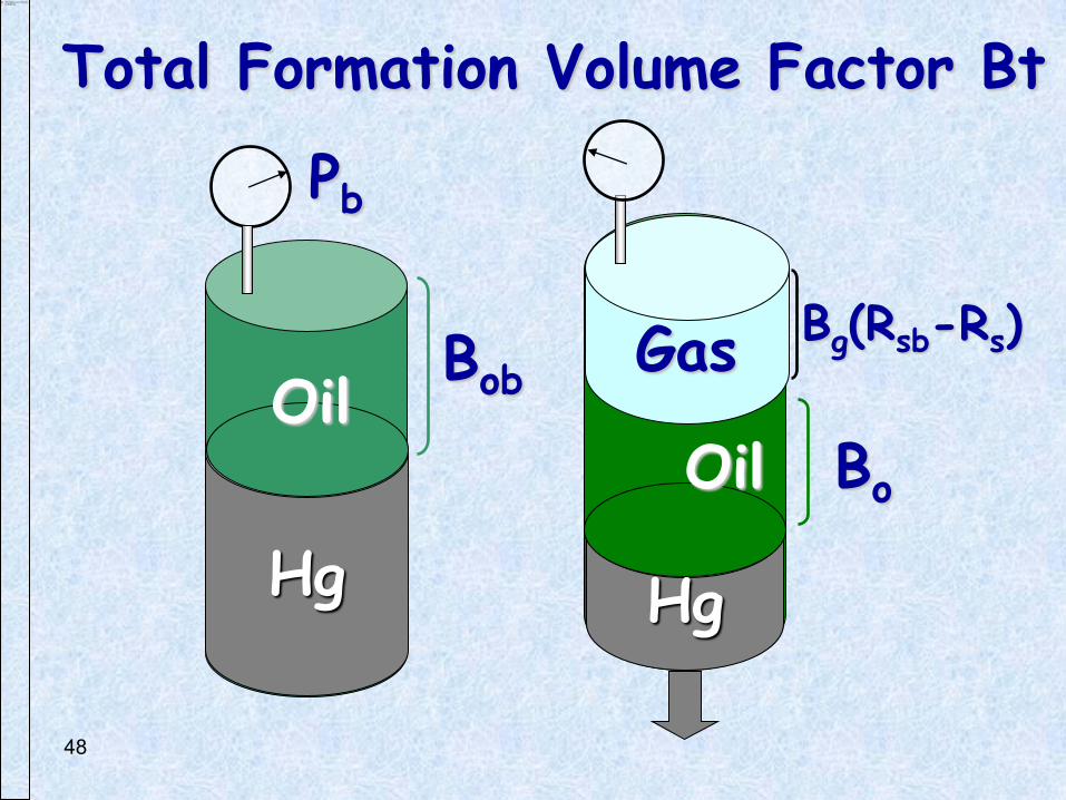
Total Formation Volume Factor Bt
Hg
Oil Bob
Hg
Gas
Oil Bo
Bg(Rsb-Rs)
Pb
48
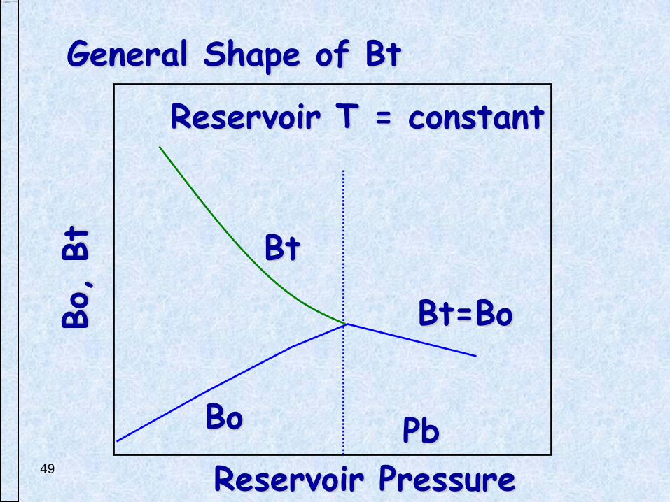
General Shape of Bt Bo,
Bt
Reservoir Pressure
Pb
Reservoir T = constant
Bt=Bo
Bt
Bo
49
50
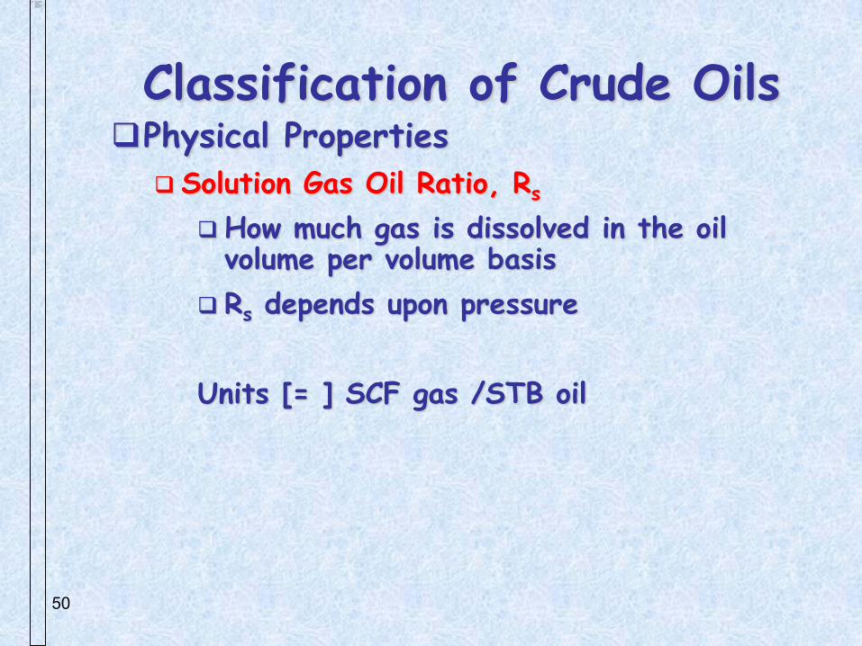
Classification of Crude Oils Physical Properties
Solution Gas Oil Ratio, Rs
How much gas is dissolved in the oil volume per volume basis
Rs depends upon pressure
Units [= ] SCF gas /STB oil
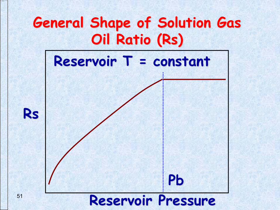
General Shape of Solution Gas Oil Ratio (Rs)
Rs
Reservoir Pressure
Pb
Reservoir T = constant
51
52
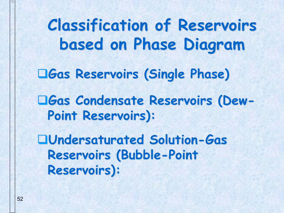
Classification of Reservoirs based on Phase Diagram
Gas Reservoirs (Single Phase)
Gas Condensate Reservoirs (Dew-Point Reservoirs):
Undersaturated Solution-Gas Reservoirs (Bubble-Point Reservoirs):
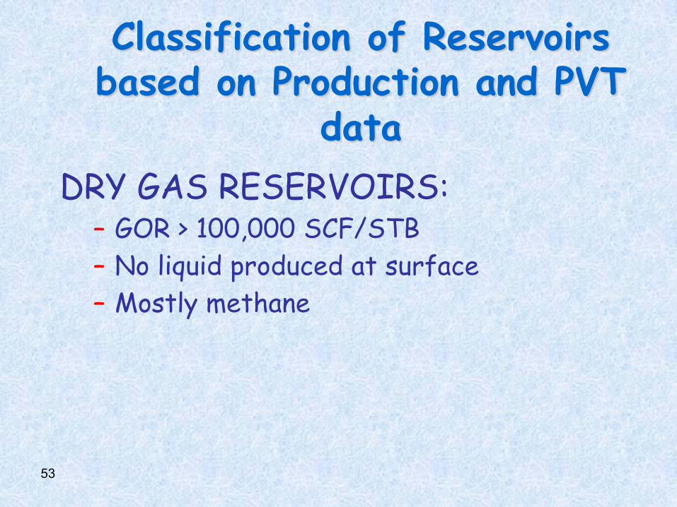
DRY GAS RESERVOIRS: – GOR > 100,000 SCF/STB
– No liquid produced at surface
– Mostly methane
53
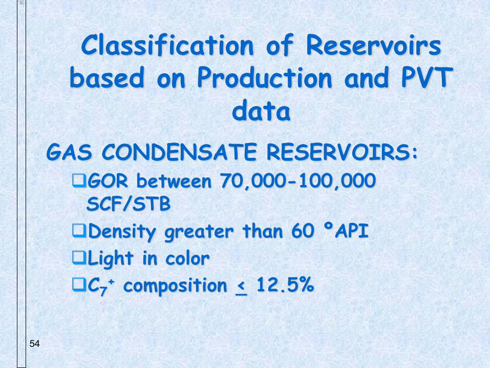
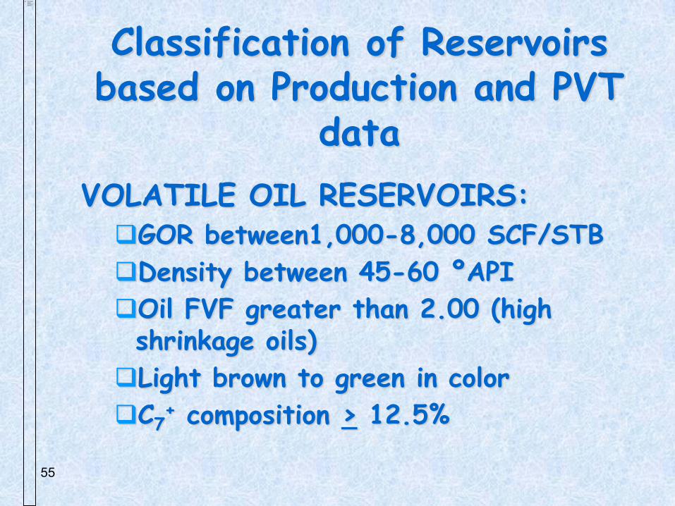
Classification of Reservoirs based on Production and PVT
data
54
Classification of Reservoirs based on Production and PVT
data
GAS CONDENSATE RESERVOIRS: GOR between 70,000-100,000 SCF/STB
Density greater than 60 ºAPI
Light in color
C7+ composition < 12.5%
55
Classification of Reservoirs based on Production and PVT
data
VOLATILE OIL RESERVOIRS: GOR between1,000-8,000 SCF/STB
Density between 45-60 ºAPI
Oil FVF greater than 2.00 (high shrinkage oils)
Light brown to green in color
C7+ composition > 12.5%
56
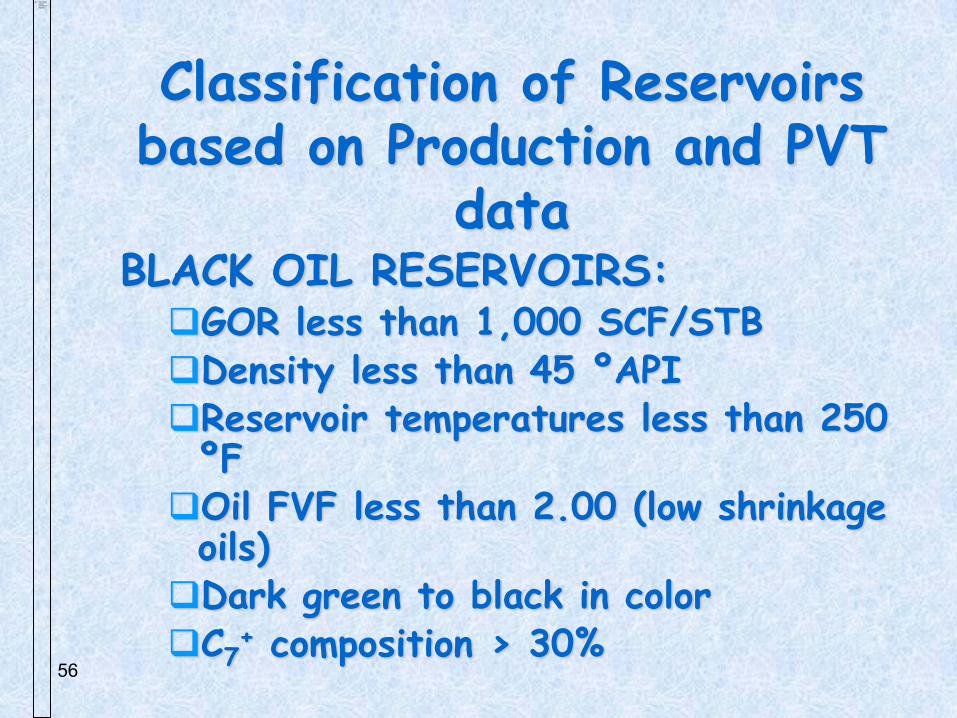
BLACK OIL RESERVOIRS: GOR less than 1,000 SCF/STB Density less than 45 ºAPI Reservoir temperatures less than 250 ºF
Oil FVF less than 2.00 (low shrinkage oils)
Dark green to black in color C7
+ composition > 30%
Classification of Reservoirs based on Production and PVT
data

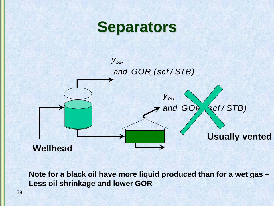
Separators
iSTx
)STB/scf( GOR and
y iST
)STB/scf( GOR and
y iSP
iSTx
Wellhead
iSPx
SToilgas
STgas
v
SToilgasSPoil
SPoilgas
SPgas
v
molelbmolelb
molelbf
molelbmolelbmolelb
molelbmolelb
molelbf
ST
SP
57
Separators
)STB/scf( GOR and
y iST
)STB/scf( GOR and
y iSP
iSTx
Wellhead
Usually vented
Note for a black oil have more liquid produced than for a wet gas –
Less oil shrinkage and lower GOR 58
PETE 310
Lecture # 17
Chapter 10 – Properties of Black Oils - Reservoir Fluid Studies
59
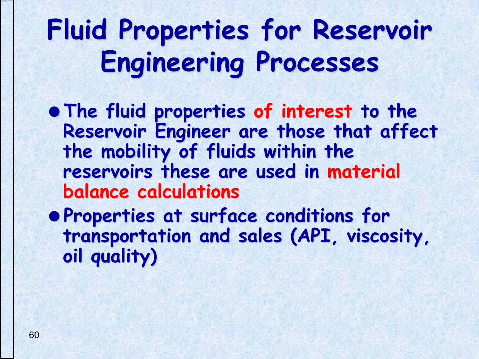
Fluid Properties for Reservoir Engineering Processes
The fluid properties of interest to the Reservoir Engineer are those that affect the mobility of fluids within the reservoirs these are used in material balance calculations Properties at surface conditions for
transportation and sales (API, viscosity, oil quality)
60
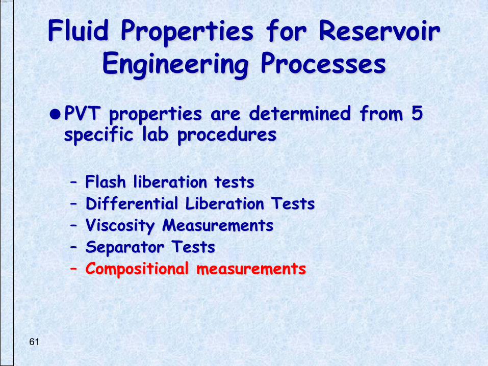
Fluid Properties for Reservoir Engineering Processes
PVT properties are determined from 5 specific lab procedures
– Flash liberation tests – Differential Liberation Tests – Viscosity Measurements – Separator Tests – Compositional measurements
61
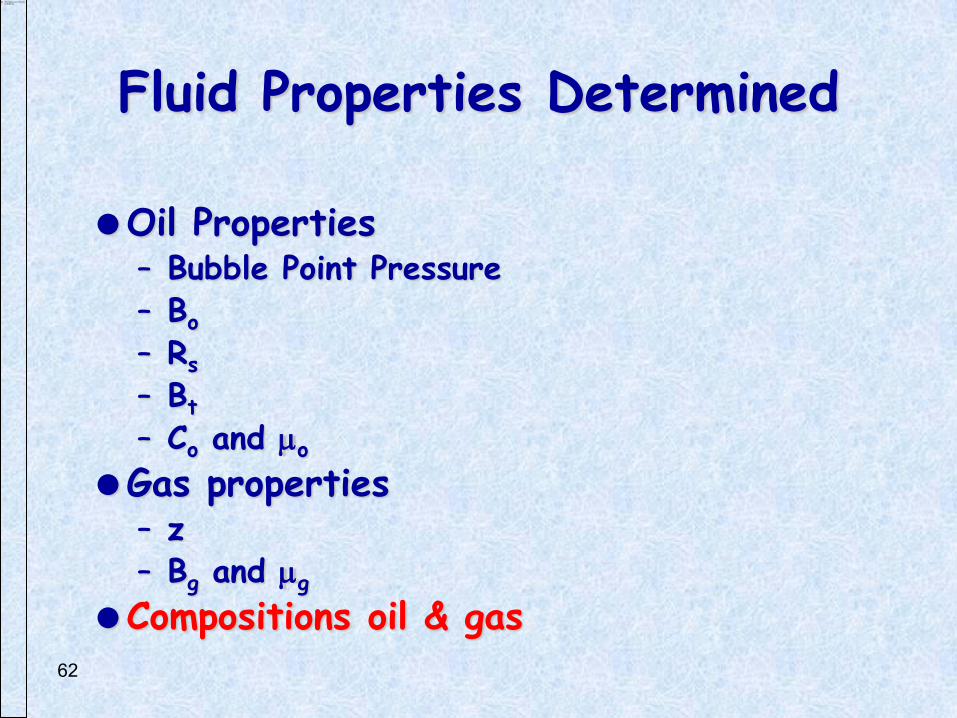
Fluid Properties Determined
Oil Properties – Bubble Point Pressure – Bo
– Rs
– Bt
– Co and mo
Gas properties – z – Bg and mg
Compositions oil & gas
62
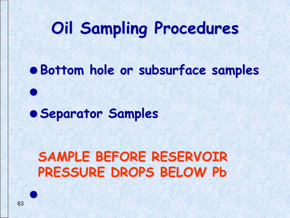
Oil Sampling Procedures
Bottom hole or subsurface samples
Separator Samples
SAMPLE BEFORE RESERVOIR PRESSURE DROPS BELOW Pb
63
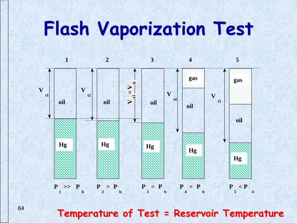
Flash Vaporization Test
Temperature of Test = Reservoir Temperature
V t1
V t2
V t3
= V
b
V t5
V t4
oil oil oil oil
oil
gas gas
Hg Hg Hg Hg
Hg
P 1 >> P
b P
2 > P
b P
3 = P
b P
4 < P
b P
5 < P
4
1 2 3 4 5
64

Flash Vaporization Test
Properties determined
– Pb
– Co
65
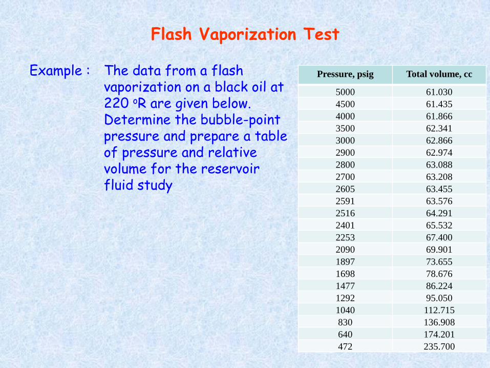
Flash Vaporization Test
Example : The data from a flash vaporization on a black oil at 220 oR are given below. Determine the bubble-point pressure and prepare a table of pressure and relative volume for the reservoir fluid study
Pressure, psig Total volume, cc
5000 61.030
4500 61.435
4000 61.866
3500 62.341
3000 62.866
2900 62.974
2800 63.088
2700 63.208
2605 63.455
2591 63.576
2516 64.291
2401 65.532
2253 67.400
2090 69.901
1897 73.655
1698 78.676
1477 86.224
1292 95.050
1040 112.715
830 136.908
640 174.201
472 235.700
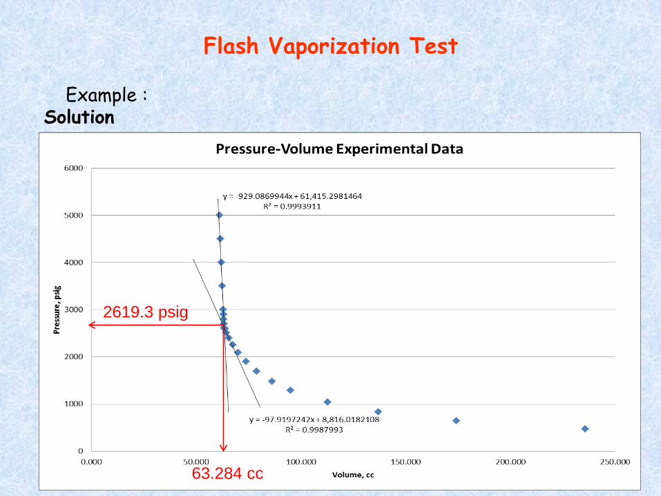
Flash Vaporization Test
Example : Solution
2619.3 psig
63.284 cc
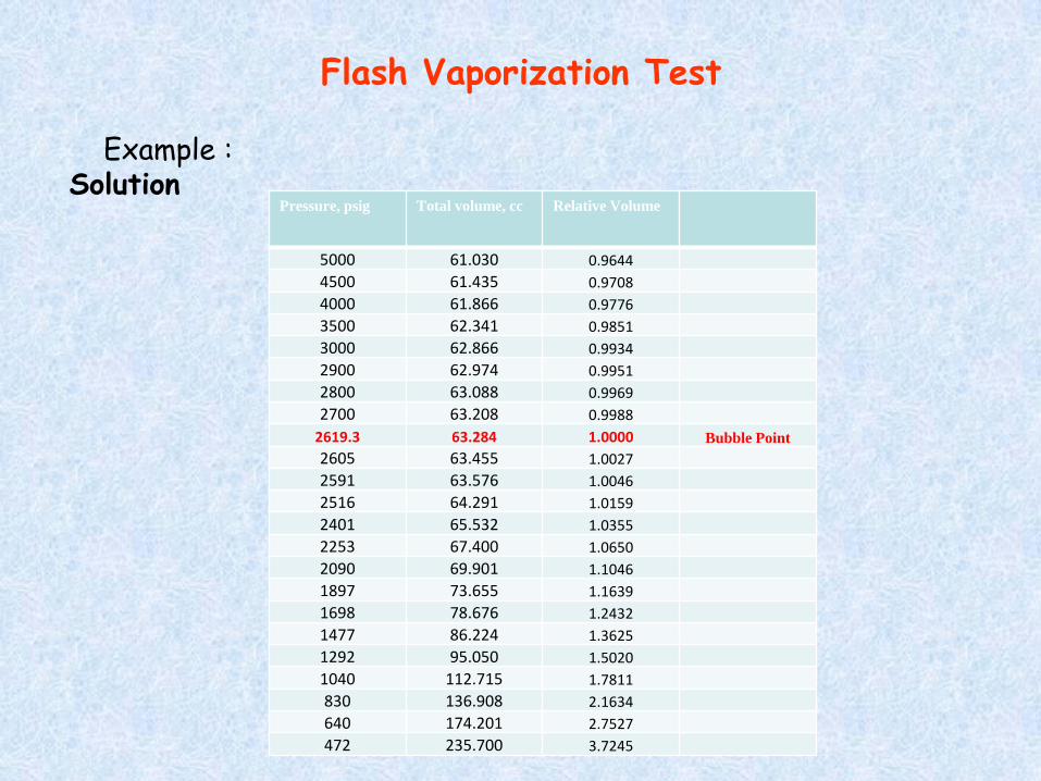
Flash Vaporization Test
Example : Solution
Pressure, psig Total volume, cc Relative Volume
5000 61.030 0.9644
4500 61.435 0.9708
4000 61.866 0.9776
3500 62.341 0.9851
3000 62.866 0.9934
2900 62.974 0.9951
2800 63.088 0.9969
2700 63.208 0.9988
2619.3 63.284 1.0000 Bubble Point
2605 63.455 1.0027
2591 63.576 1.0046
2516 64.291 1.0159
2401 65.532 1.0355
2253 67.400 1.0650
2090 69.901 1.1046
1897 73.655 1.1639
1698 78.676 1.2432
1477 86.224 1.3625
1292 95.050 1.5020
1040 112.715 1.7811
830 136.908 2.1634
640 174.201 2.7527
472 235.700 3.7245
Lecture 2.1: Continuity and Bernoulli’s Equation
Incompressible Fluid Flow
• Today’s Lecture
– Volume and Mass Flow Rate
– Continuity equation
– Energy in a fluid
– Flow Work
– Bernoulli’s Equation
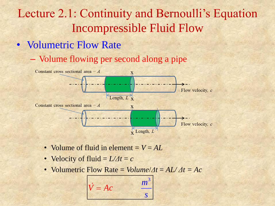
Lecture 2.1: Continuity and Bernoulli’s Equation
Incompressible Fluid Flow
• Volumetric Flow Rate
– Volume flowing per second along a pipe
• Volume of fluid in element = V = AL
• Velocity of fluid = L/Δt = c
• Volumetric Flow Rate = Volume/Δt = AL/ Δt = Ac
3
sV Ac
m
Lecture 2.1: Continuity and Bernoulli’s Equation
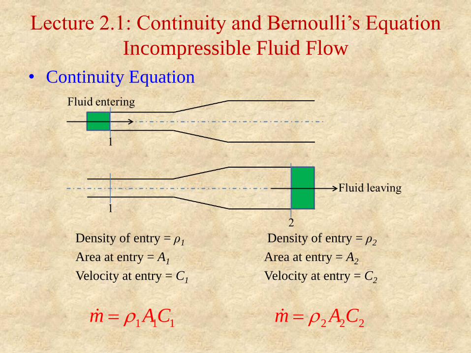
Incompressible Fluid Flow
• Continuity Equation
Density of entry = ρ1 Density of entry = ρ2
Area at entry = A1 Area at entry = A2
Velocity at entry = C1 Velocity at entry = C2
1 1 1m AC 2 2 2m A C
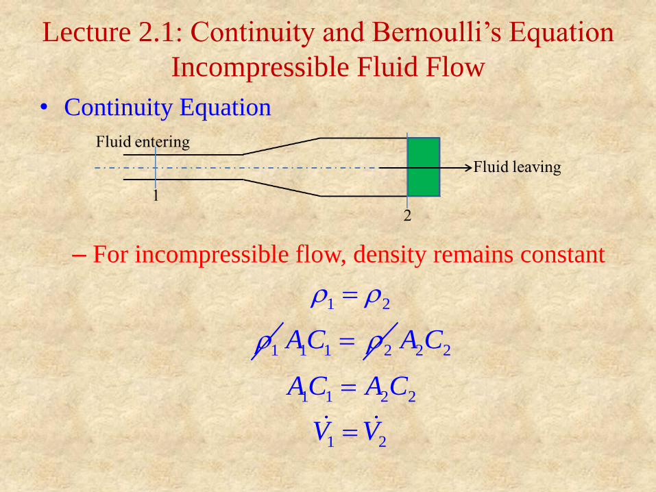
Lecture 2.1: Continuity and Bernoulli’s Equation
Incompressible Fluid Flow
• Continuity Equation
– For incompressible flow, density remains constant
1 2
1
1 1 2AC 2 2
1 1 2 2
1 2
A C
AC A C
V V
Lecture 2.1: Continuity and Bernoulli’s Equation
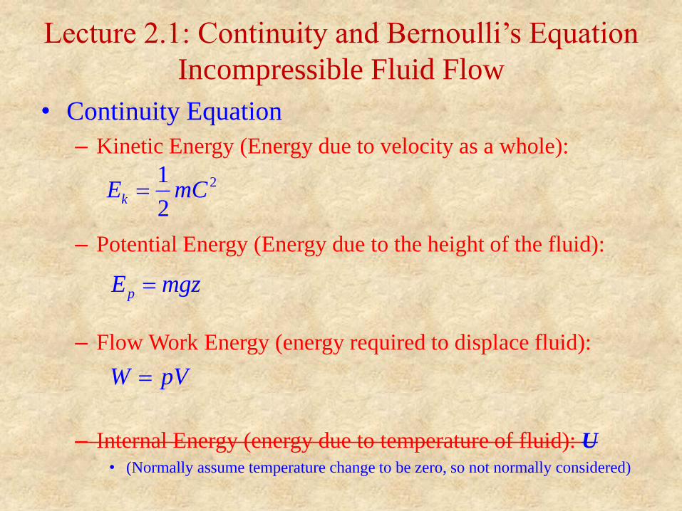
Incompressible Fluid Flow
• Continuity Equation
– Kinetic Energy (Energy due to velocity as a whole):
– Potential Energy (Energy due to the height of the fluid):
– Flow Work Energy (energy required to displace fluid):
– Internal Energy (energy due to temperature of fluid): U • (Normally assume temperature change to be zero, so not normally considered)
21
2kE mC
pE mgz
W pV
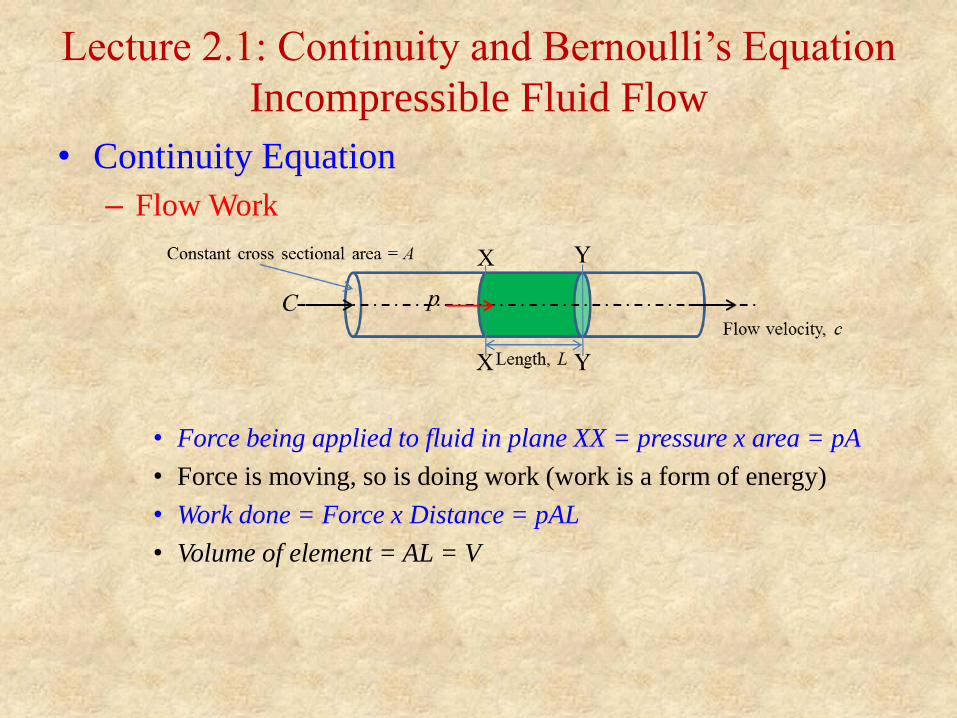
Lecture 2.1: Continuity and Bernoulli’s Equation
Incompressible Fluid Flow
• Continuity Equation
– Flow Work
• Force being applied to fluid in plane XX = pressure x area = pA
• Force is moving, so is doing work (work is a form of energy)
• Work done = Force x Distance = pAL
• Volume of element = AL = V
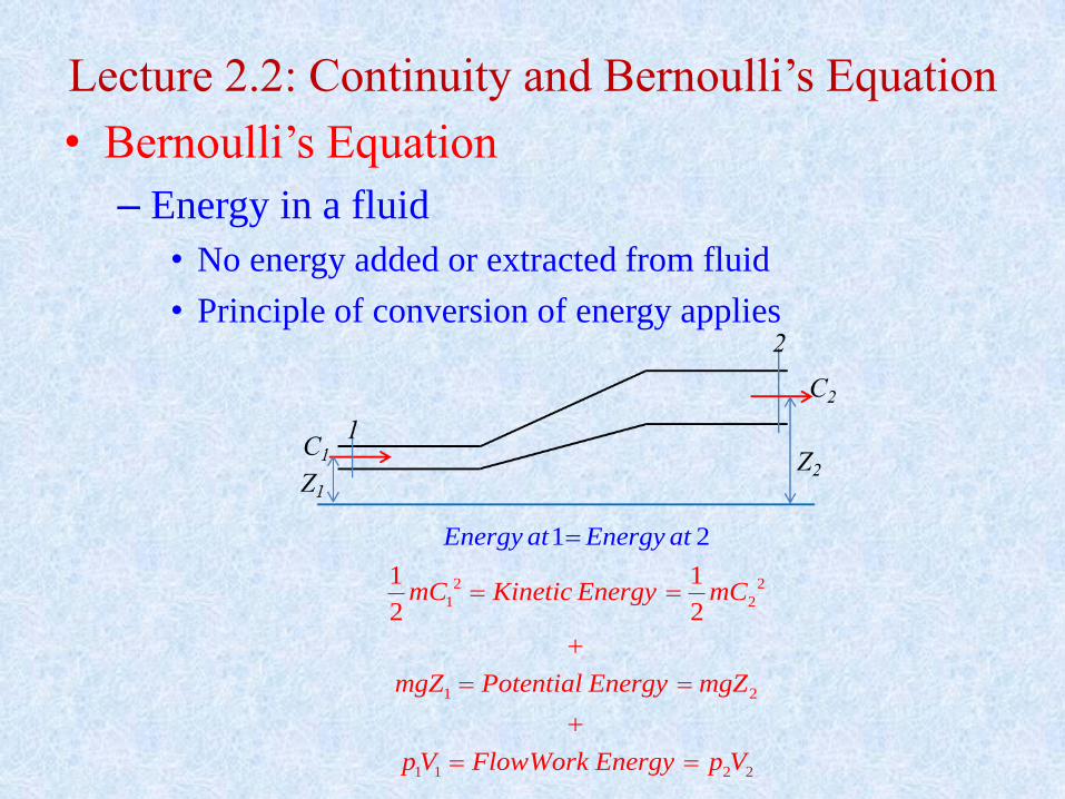
Lecture 2.2: Continuity and Bernoulli’s Equation
• Bernoulli’s Equation
– Energy in a fluid
• No energy added or extracted from fluid
• Principle of conversion of energy applies
2 2
1 2
1 2
1 1 2 2
1 1
2
1 2
2mC Kinetic Energy mC
mgZ Potential Energy
Energ
mgZ
p V
y at Ener
Flo
gy a
wWork Energy p
t
V
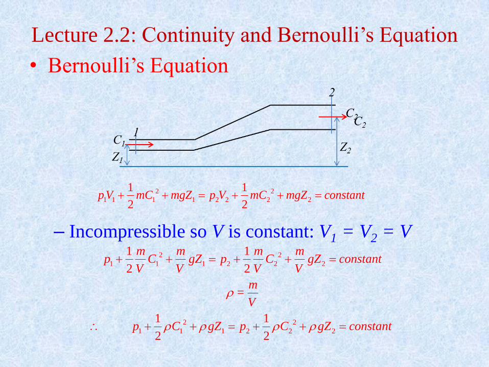
Lecture 2.2: Continuity and Bernoulli’s Equation
• Bernoulli’s Equation
– Incompressible so V is constant: V1 = V2 = V
2 2
1 1 1 1 2 2 2 2
1 1
2 2p V mC mgZ p V mC mgZ constant
2 2
1 1 1 2 2 2
2 2
1 1 1 2 2 2
1 1
2 2
1 1
2 2
m m m mp C gZ p C gZ constant
V V V V
m=
V
p C gZ p C gZ constant
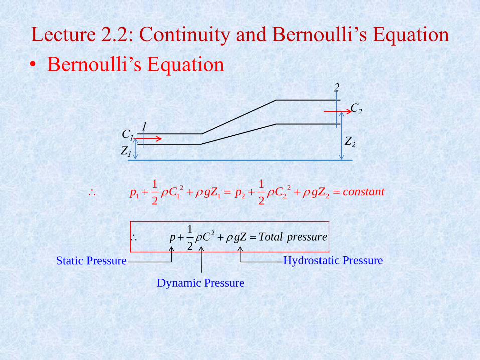
Lecture 2.2: Continuity and Bernoulli’s Equation
• Bernoulli’s Equation
2 2
1 1 1 2 2 2
1 1
2 2p C gZ p C gZ constant
21
2p C gZ Total pressure
Static Pressure Hydrostatic Pressure
Dynamic Pressure
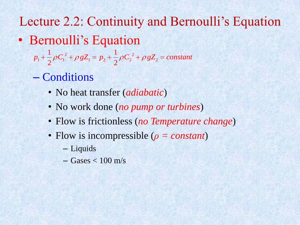
Lecture 2.2: Continuity and Bernoulli’s Equation
• Bernoulli’s Equation
– Conditions
• No heat transfer (adiabatic)
• No work done (no pump or turbines)
• Flow is frictionless (no Temperature change)
• Flow is incompressible (ρ = constant)
– Liquids
– Gases < 100 m/s
2 2
1 1 1 2 2 2
1 1
2 2p C gZ p C gZ constant
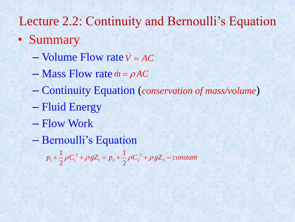
Lecture 2.2: Continuity and Bernoulli’s Equation
• Summary
– Volume Flow rate
– Mass Flow rate
– Continuity Equation (conservation of mass/volume)
– Fluid Energy
– Flow Work
– Bernoulli’s Equation
V AC
m AC
2 2
1 1 1 2 2 2
1 1
2 2p C gZ p C gZ constant
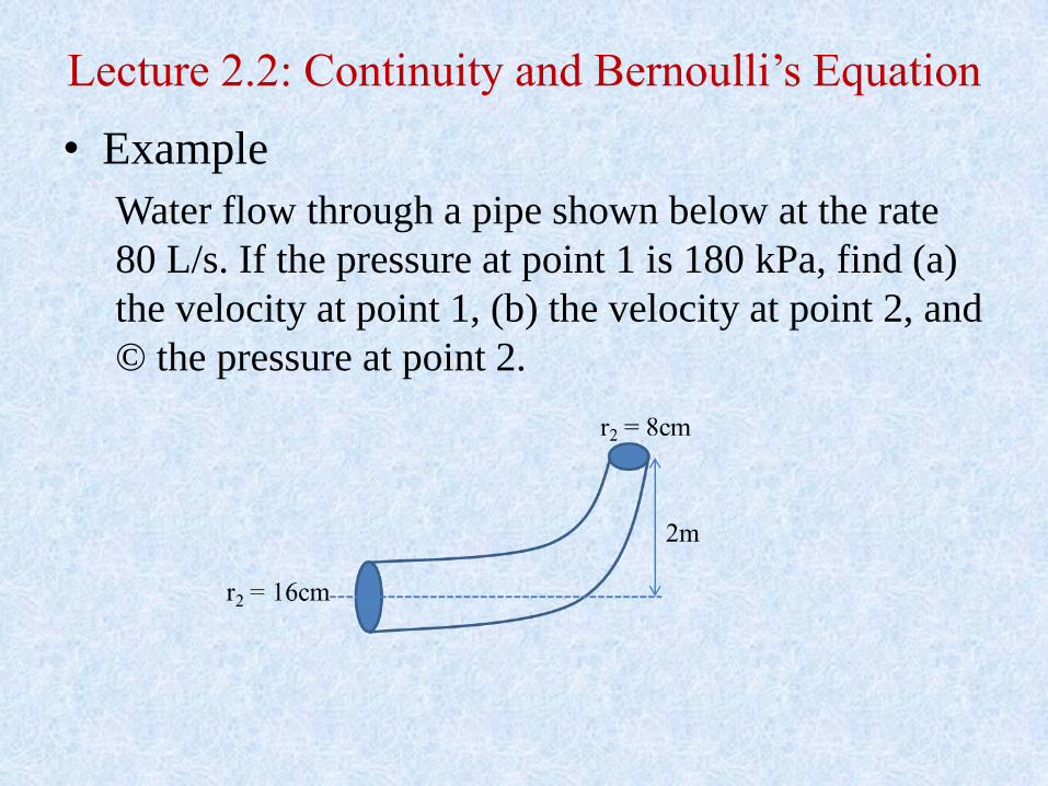
Lecture 2.2: Continuity and Bernoulli’s Equation
• Example
Water flow through a pipe shown below at the rate
80 L/s. If the pressure at point 1 is 180 kPa, find (a)
the velocity at point 1, (b) the velocity at point 2, and
© the pressure at point 2.
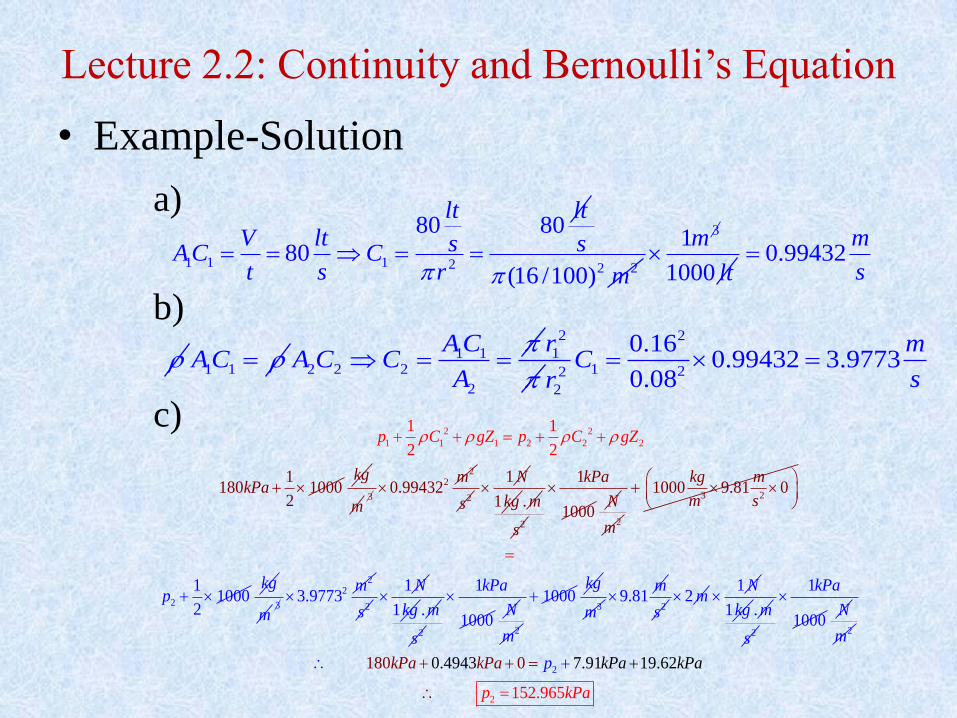
Lecture 2.2: Continuity and Bernoulli’s Equation
• Example-Solution
a)
b)
c)
1 1 1 2
80 80
80
lt lt
V lt sAC Ct s r
2 2(16 /100)
s
m
31m
1000 lt0.99432
m
s
1 1AC 1 12 2 2
2
ACA C C
A
2
1r
2
1 22
2
0.160.99432 3.9773
0.08
mC
sr
2 2
1 1 1 2 2 2
1180 100
1
02
1
2 2p C gZ p C
a
gZ
kP
kg
m3
220.99432
m
2s
1 N
1kg . m
2s
1
1000
kPa
N2m
3 21000 9.81 0
kg m
m s
2
11000
2p
kg
m3
223.9773
m
2s
1 N
1kg . m
2s
1
1000
kPa
N2m
1000kg
3m9.81
m
2s2 m
1 N
1kg . m
2s
1
1000
kPa
N2m
2
2
0.4943 7.91 19.6180 0
152.
2
965
kPa kP kPa
p
Pa
a
p a
kP
k
Lecture 2.2: Continuity and Bernoulli’s Equation
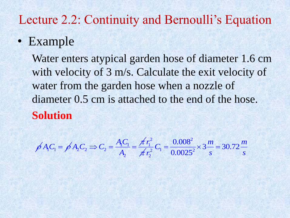
• Example
Water enters atypical garden hose of diameter 1.6 cm
with velocity of 3 m/s. Calculate the exit velocity of
water from the garden hose when a nozzle of
diameter 0.5 cm is attached to the end of the hose.
Solution
1 1AC 1 12 2 2
2
ACA C C
A
2
1r
2
1 22
2
0.0083 30.72
0.0025
m mC
s sr
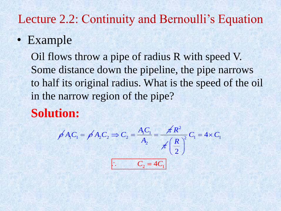
Lecture 2.2: Continuity and Bernoulli’s Equation
• Example
Oil flows throw a pipe of radius R with speed V.
Some distance down the pipeline, the pipe narrows
to half its original radius. What is the speed of the oil
in the narrow region of the pipe?
Solution:
1 1AC 1 12 2 2
2
ACA C C
A
2R
12
2 1
14
2
4C
C CR
C
Lecture 1.1 flow with Friction & Laminar Flow
Part I: Introduction, Fluid Flow with Friction & Type of Flow
• Today’s Lecture – Fluid flow with friction – Nature of flows: Laminar and Turbulent – Shear Stress and Fluid Viscosity – Laminar Flow
• Flow Velocity • Flow Rate • Pressure drop • Power
– Example
Lecture 1.1 flow with Friction & Laminar Flow
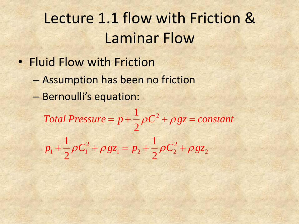
• Fluid Flow with Friction
– Assumption has been no friction
– Bernoulli’s equation:
2
2 2
1 1 1 2 2 2
1
2
1 1
2 2
Total Pressure p C gz constant
p C gz p C gz
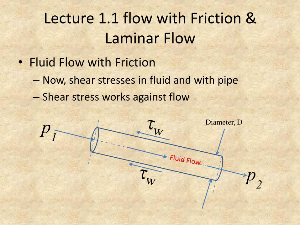
Lecture 1.1 flow with Friction & Laminar Flow
• Fluid Flow with Friction
– Now, shear stresses in fluid and with pipe
– Shear stress works against flow
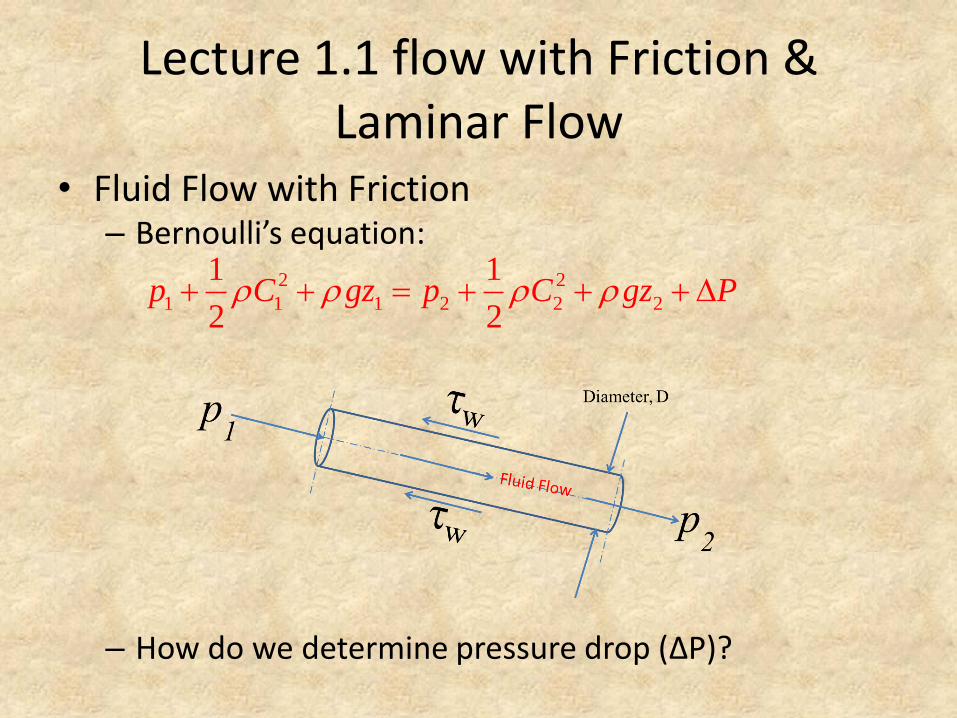
Lecture 1.1 flow with Friction & Laminar Flow
• Fluid Flow with Friction – Bernoulli’s equation:
– How do we determine pressure drop (ΔP)?
2 2
1 1 1 2 2 2
1 1
2 2p C gz p C gz P
Lecture 1.1 flow with Friction &
Laminar Flow
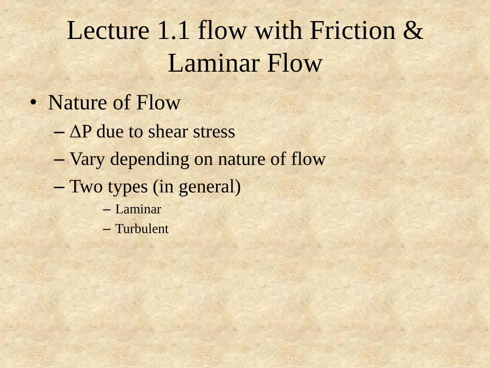
• Nature of Flow
– ΔP due to shear stress
– Vary depending on nature of flow
– Two types (in general) – Laminar
– Turbulent
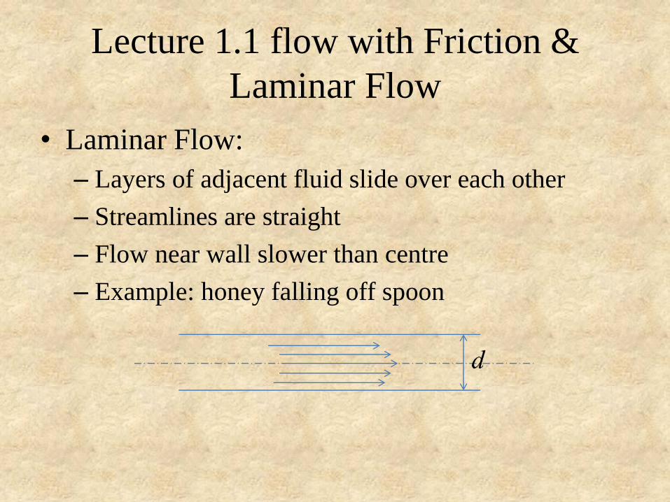
Lecture 1.1 flow with Friction &
Laminar Flow
• Laminar Flow:
– Layers of adjacent fluid slide over each other
– Streamlines are straight
– Flow near wall slower than centre
– Example: honey falling off spoon
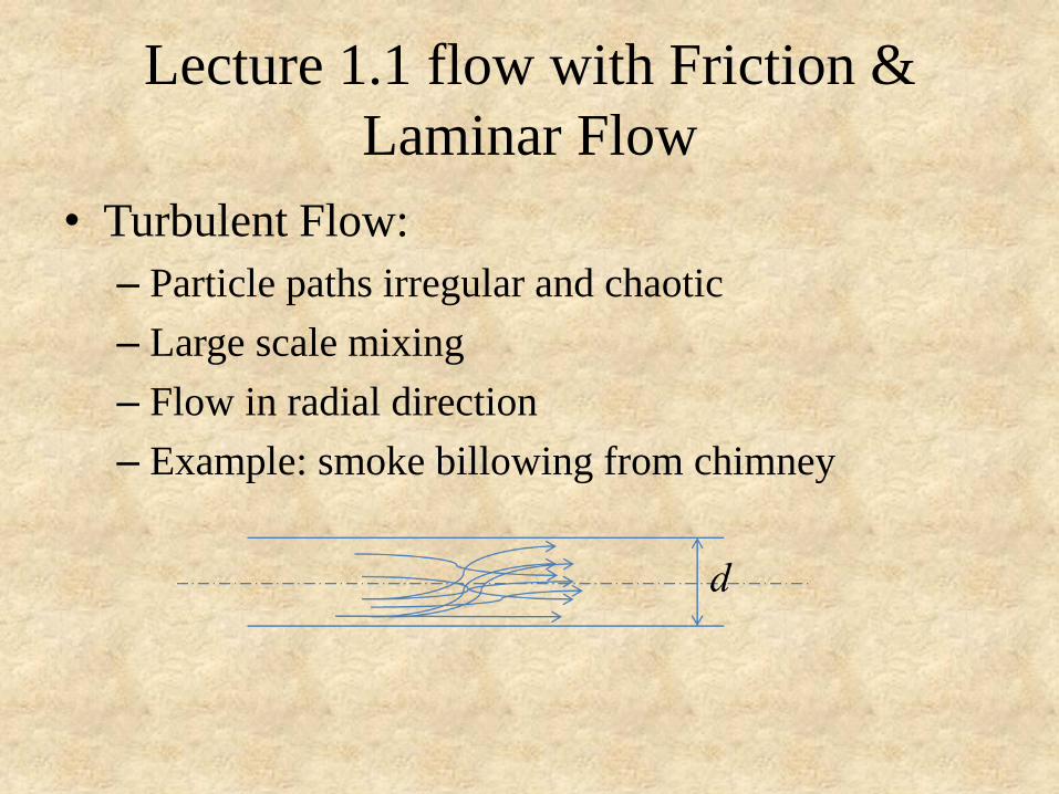
Lecture 1.1 flow with Friction &
Laminar Flow
• Turbulent Flow:
– Particle paths irregular and chaotic
– Large scale mixing
– Flow in radial direction
– Example: smoke billowing from chimney
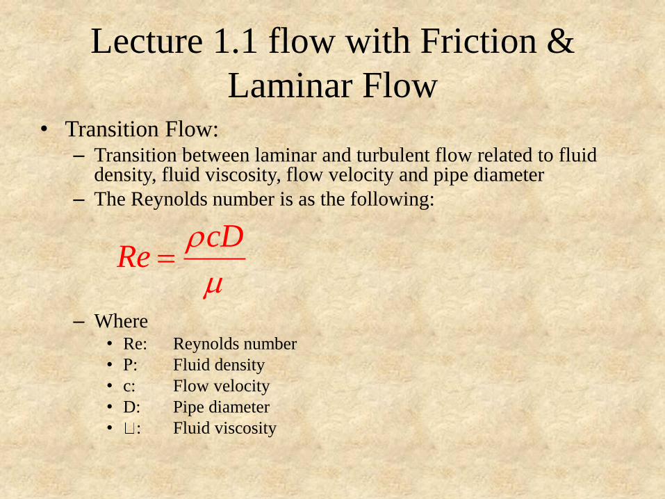
Lecture 1.1 flow with Friction &
Laminar Flow • Transition Flow:
– Transition between laminar and turbulent flow related to fluid density, fluid viscosity, flow velocity and pipe diameter
– The Reynolds number is as the following:
– Where • Re: Reynolds number
• Ρ: Fluid density
• c: Flow velocity
• D: Pipe diameter
• : Fluid viscosity
cDRe
m
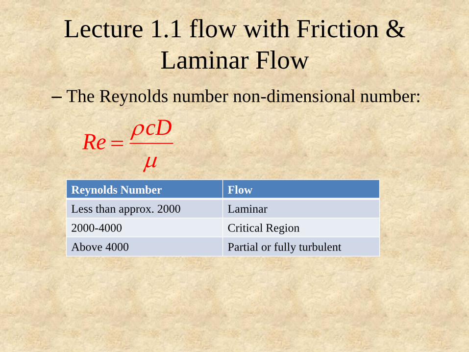
Lecture 1.1 flow with Friction &
Laminar Flow
– The Reynolds number non-dimensional number:
cDRe
m
Reynolds Number Flow
Less than approx. 2000 Laminar
2000-4000 Critical Region
Above 4000 Partial or fully turbulent
Lecture 1.2 flow with Friction &
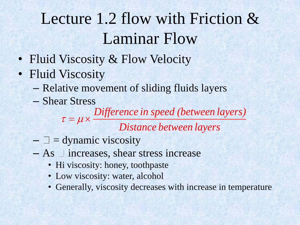
Laminar Flow
• Fluid Viscosity & Flow Velocity
• Fluid Viscosity – Relative movement of sliding fluids layers
– Shear Stress
– = dynamic viscosity
– As increases, shear stress increase • Hi viscosity: honey, toothpaste
• Low viscosity: water, alcohol
• Generally, viscosity decreases with increase in temperature
Difference in speed (between layers)
Distance between layers m
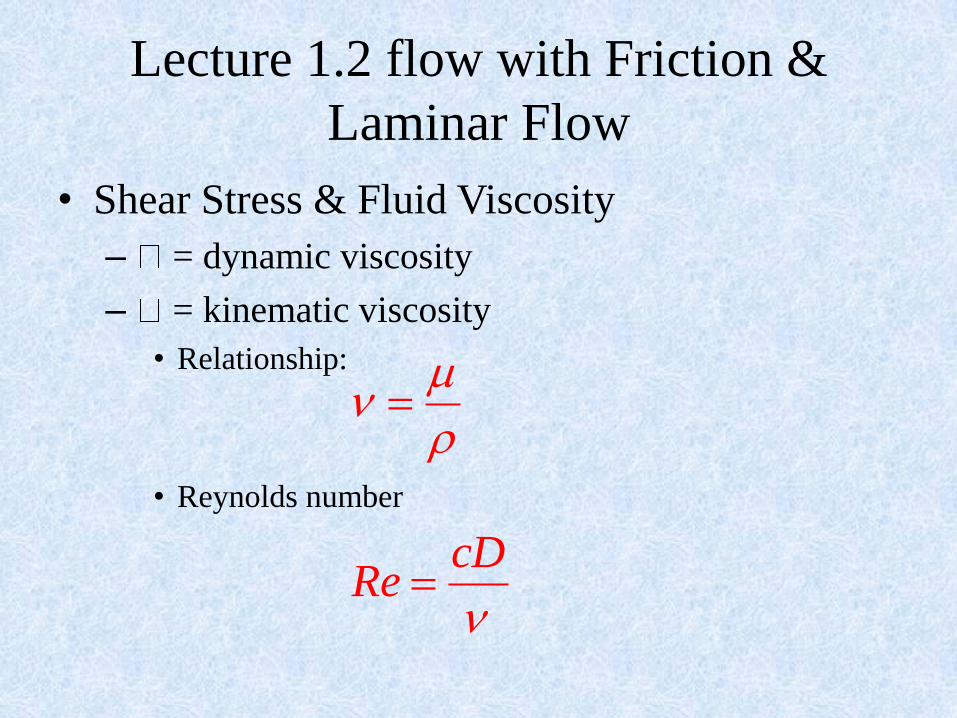
Lecture 1.2 flow with Friction &
Laminar Flow
• Shear Stress & Fluid Viscosity
– = dynamic viscosity
– = kinematic viscosity
• Relationship:
• Reynolds number
cD
Re
m
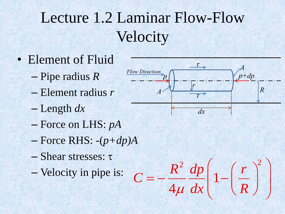
Lecture 1.2 Laminar Flow-Flow
Velocity
• Element of Fluid
– Pipe radius R
– Element radius r
– Length dx
– Force on LHS: pA
– Force RHS: -(p+dp)A
– Shear stresses:
– Velocity in pipe is: 22
14
R dp rC
dx Rm

Lecture 1.2 Laminar Flow-Flow
Velocity
• Velocity:
– Quadratic equation
– Parabolic velocity profile
– If r = R
• Velocity = 0
– If r = 0
• Velocity = Cmax
22
14
R dp rC
dx Rm
Pipe walls
Flo
w D
irec
tio
n
Cen
ter
lin
e o
f p
ipe
Cmix
0 0
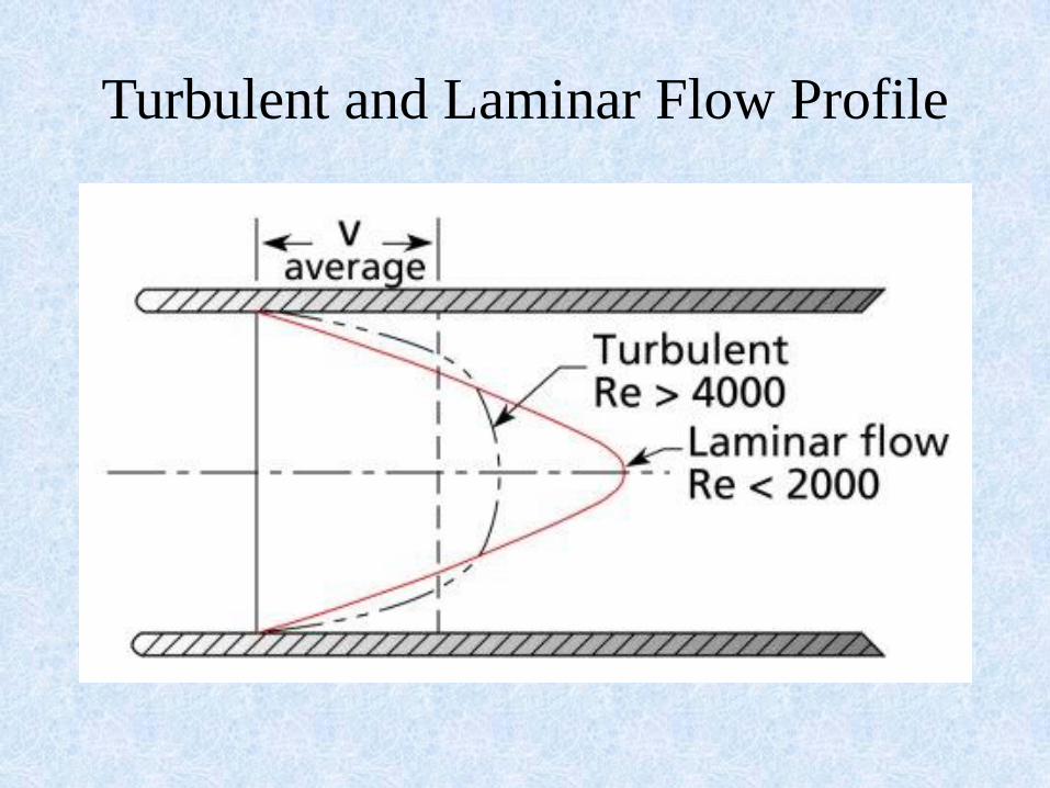
Turbulent and Laminar Flow Profile
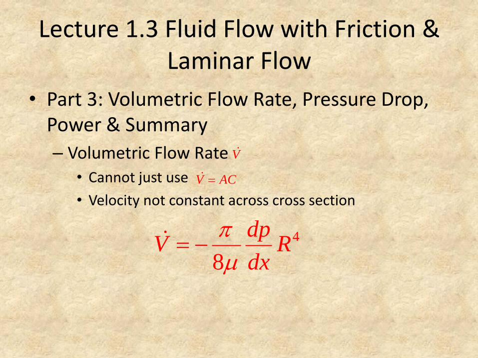
Lecture 1.3 Fluid Flow with Friction & Laminar Flow
• Part 3: Volumetric Flow Rate, Pressure Drop, Power & Summary
– Volumetric Flow Rate
• Cannot just use
• Velocity not constant across cross section
V AC
4
8
dpV R
dx
m
V
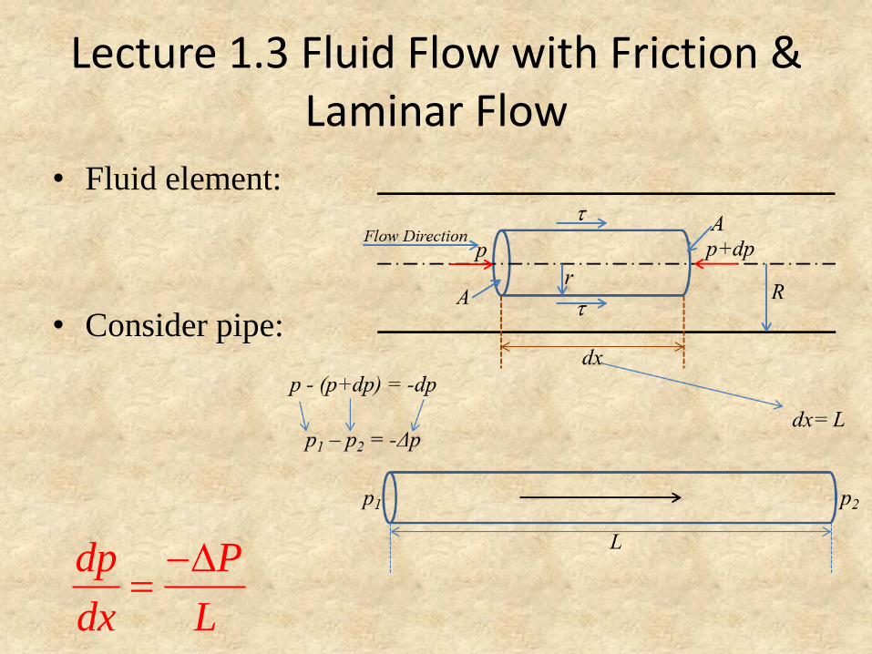
Lecture 1.3 Fluid Flow with Friction & Laminar Flow
• Fluid element:
• Consider pipe:
dp P
dx L
Lecture 1.3 Laminar Flow-Pressure
Drop
• Using:
• Velocity:
• Flow rate: 4 4
8 8
dpV R
dx
PV R
L
mm
dp P
dx L
22 22
14
14
R dp r R P rC
L RC
dx R mm
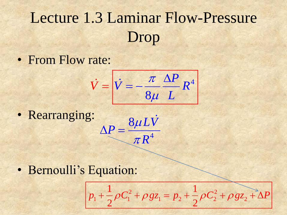
Lecture 1.3 Laminar Flow-Pressure
Drop
• From Flow rate:
• Rearranging:
• Bernoulli’s Equation:
4
8V
PV R
L
m
4
8 LVP
R
m
2 2
1 1 1 2 2 2
1 1
2 2p C gz p C gz P
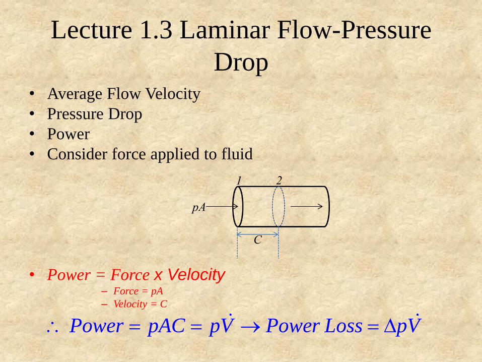
Lecture 1.3 Laminar Flow-Pressure
Drop • Average Flow Velocity
• Pressure Drop
• Power
• Consider force applied to fluid
• Power = Force x Velocity – Force = pA
– Velocity = C
Power pAC pV Power Loss pV
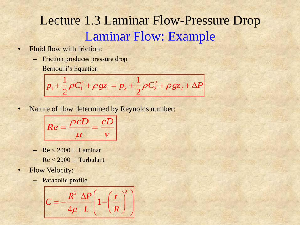
Lecture 1.3 Laminar Flow-Pressure Drop
Laminar Flow: Example • Fluid flow with friction:
– Friction produces pressure drop
– Bernoulli’s Equation
• Nature of flow determined by Reynolds number:
– Re < 2000 Laminar
– Re < 2000 Turbulant
• Flow Velocity:
– Parabolic profile
2 2
1 1 1 2 2 2
1 1
2 2p C gz p C gz P
cD cDRe
m
22
14
R P rC
L Rm
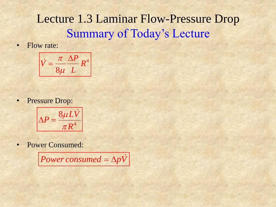
Lecture 1.3 Laminar Flow-Pressure Drop
Summary of Today’s Lecture • Flow rate:
• Pressure Drop:
• Power Consumed:
Power consumed pV
4
8 LVP
R
m
4
8
PV R
L
m

Lecture 1.3 Laminar Flow-Pressure Drop
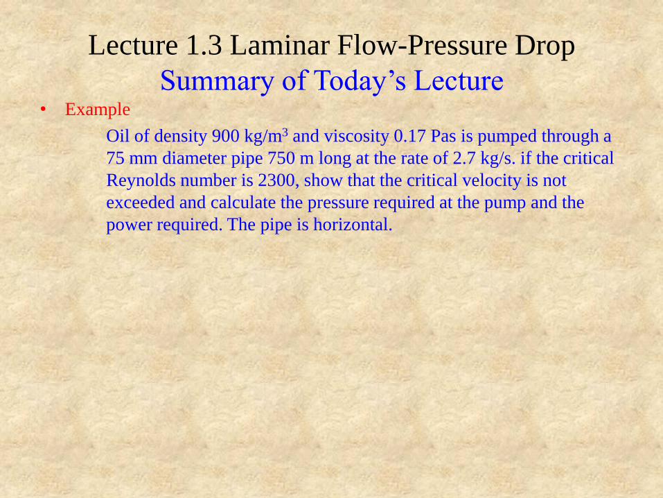
Summary of Today’s Lecture • Example
Oil of density 900 kg/m3 and viscosity 0.17 Pas is pumped through a
75 mm diameter pipe 750 m long at the rate of 2.7 kg/s. if the critical
Reynolds number is 2300, show that the critical velocity is not
exceeded and calculate the pressure required at the pump and the
power required. The pipe is horizontal.
Lecture 1.3 Laminar Flow-Pressure Drop
Summary of Today’s Lecture • Solution
Mass flow is given, we need velocity in order to find the Re and
volumetric flow in order to find the Δp and power
3
2
900 , 0.17 . , 75 , 750
2.7 Re 2300 ? ?
2.7
4
kgPa s D mm l m
m
kgm P power
s
kg
m mm Ac c
AD
m
900
s
kg
3m
20.0754
m
0.679
900
Re
m
s
kg
cD
m
m
30.679
m
s0.075 m
0.17 .Pa s
.Pa s
kg
m . s
The flow is l
2
a
69.
ar
6
min
Lecture 1.3 Laminar Flow-Pressure Drop
Summary of Today’s Lecture • Solution
Mass flow is given, we need velocity in order to find the Re and
volumetric flow in order to find the Δp and power
3900 , 0.17 . , 75 , 750
2.7 Re 2300 ? ?
2.7
kgPa s D mm L m
m
kgm P power
s
kg
mV
m
900
s
kg
3
3
4
0.003
8 0.17 .8
m
s
m
Pa sLV
pR
m
750 m3
0.003m
4
40.075
2
s
m
.
.
kg
m s
Pa s
2492795.5
.
492795.5
kg
m s
kgp
2.m s
1
1
N
kg
2
.m
s
2
2
492795.5
492795.5
N
m
Np
m
2
1
100000
bar
N
m
9
4.93
4. 3
bar
p bar
Lecture 1.3 Laminar Flow-Pressure Drop
Summary of Today’s Lecture • Solution
Mass flow is given, we need velocity in order to find the Re and
volumetric flow in order to find the Δp and power
3
2
900 , 0.17 . , 75 , 750
2.7 Re 2300 ? ?
492795.5
kgPa s D mm L m
m
kgm P power
s
Npower pV
m
m
3
0.003m
.
1478.4
.1478.4
N m
s s
N mpower
s
1
.1
W
N m
s
1478.4
1478.4
power W
W
Introduction and Fluids at Rest
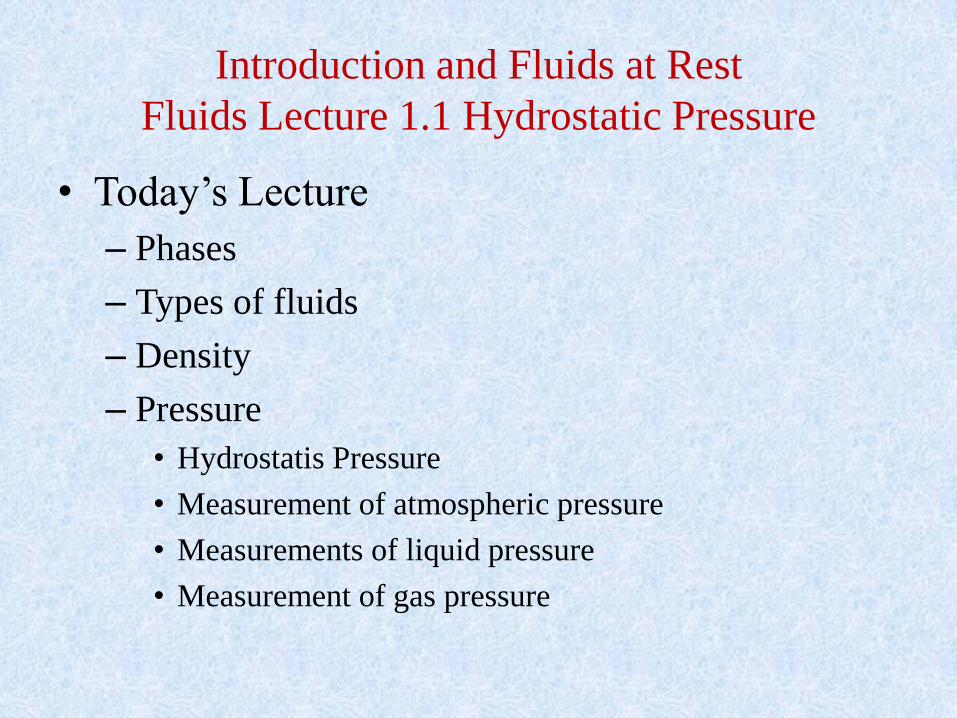
Fluids Lecture 1.1 Hydrostatic Pressure
• Today’s Lecture
– Phases
– Types of fluids
– Density
– Pressure
• Hydrostatis Pressure
• Measurement of atmospheric pressure
• Measurements of liquid pressure
• Measurement of gas pressure
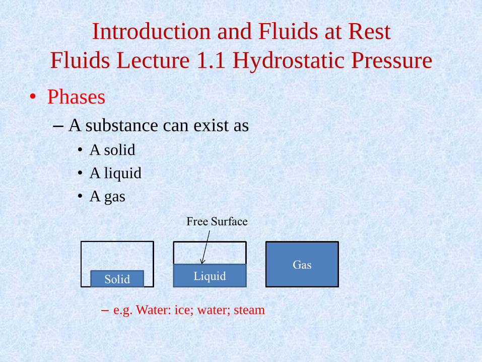
Introduction and Fluids at Rest
Fluids Lecture 1.1 Hydrostatic Pressure
• Phases
– A substance can exist as
• A solid
• A liquid
• A gas
– e.g. Water: ice; water; steam
Introduction and Fluids at Rest
Fluids Lecture 1.1 Hydrostatic Pressure
• Phases
– Solids
• Maintains shape
• Can withstand tensile (pulling), compressive and shear
sliding stress
– Fluids
• Includes liquids and gases
• Little resistance to a permanent change in shape
• Take on the shape of container
Introduction and Fluids at Rest
Fluids Lecture 1.1 Hydrostatic Pressure
• Phases
– Fluids
• Two types of fluids (generally)
– Incompressible Fluids: Liquids
» Molecules arranged so a given mass of fluid will retain
virtually the same volume irrespective of pressure
• Compressible Fluids: Gases and Vapors
– Free molecular arrangement, so tend to fill any vessel
– Pressure changes produce considerable change in volume
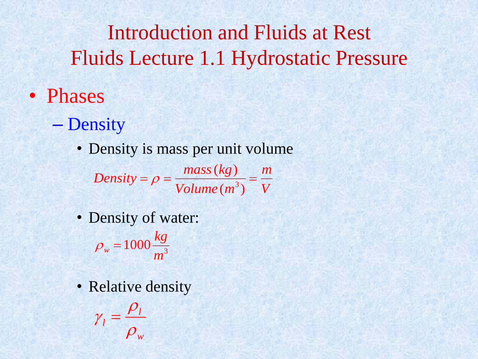
Introduction and Fluids at Rest
Fluids Lecture 1.1 Hydrostatic Pressure
• Phases
– Density
• Density is mass per unit volume
• Density of water:
• Relative density
3
( )
( )
mass kg mDensity
Volume m V
31000w
kg
m
ll
w
Introduction and Fluids at Rest
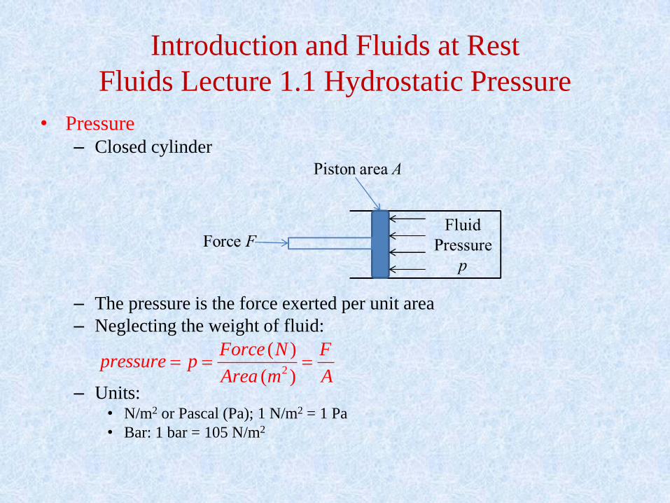
Fluids Lecture 1.1 Hydrostatic Pressure
• Pressure – Closed cylinder
– The pressure is the force exerted per unit area
– Neglecting the weight of fluid:
– Units: • N/m2 or Pascal (Pa); 1 N/m2 = 1 Pa
• Bar: 1 bar = 105 N/m2
2
( )
( )
Force N Fpressure p
Area m A
Introduction and Fluids at Rest
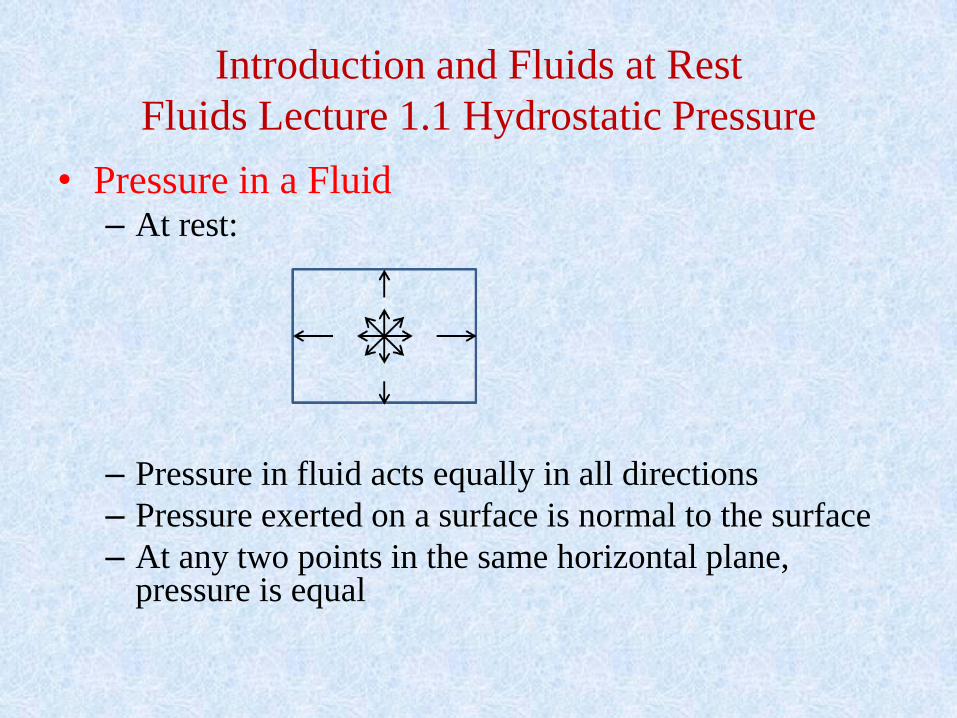
Fluids Lecture 1.1 Hydrostatic Pressure
• Pressure in a Fluid – At rest:
– Pressure in fluid acts equally in all directions
– Pressure exerted on a surface is normal to the surface
– At any two points in the same horizontal plane, pressure is equal
Introduction and Fluids at Rest
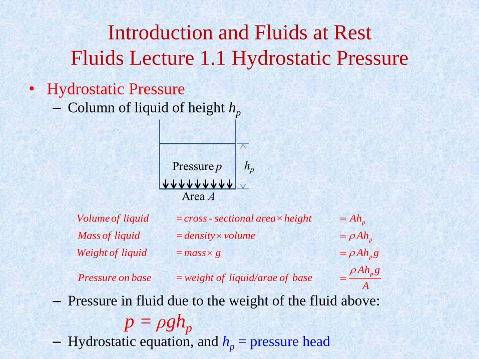
Fluids Lecture 1.1 Hydrostatic Pressure
• Hydrostatic Pressure – Column of liquid of height hp
– Pressure in fluid due to the weight of the fluid above:
p = ρghp – Hydrostatic equation, and hp = pressure head
p
p
p
p
Volumeof liquid =cross - sectional area×height Ah
Mass of liquid =density volume Ah
Weight of liquid =mass g Ah g
Ah gPressure on base = weight of liquid/arae of base
A
Introduction and Fluids at Rest
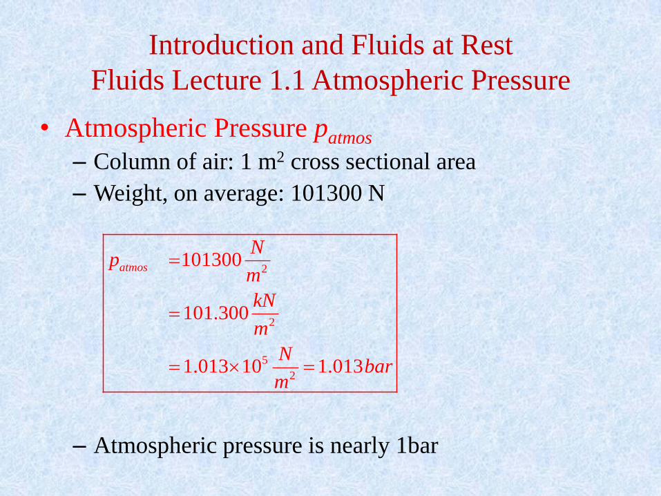
Fluids Lecture 1.1 Atmospheric Pressure
• Atmospheric Pressure patmos
– Column of air: 1 m2 cross sectional area
– Weight, on average: 101300 N
– Atmospheric pressure is nearly 1bar
2
2
5
2
101300
101.300
1.013 10 1.013
atmos
Np
m
kN
m
Nbar
m
Introduction and Fluids at Rest
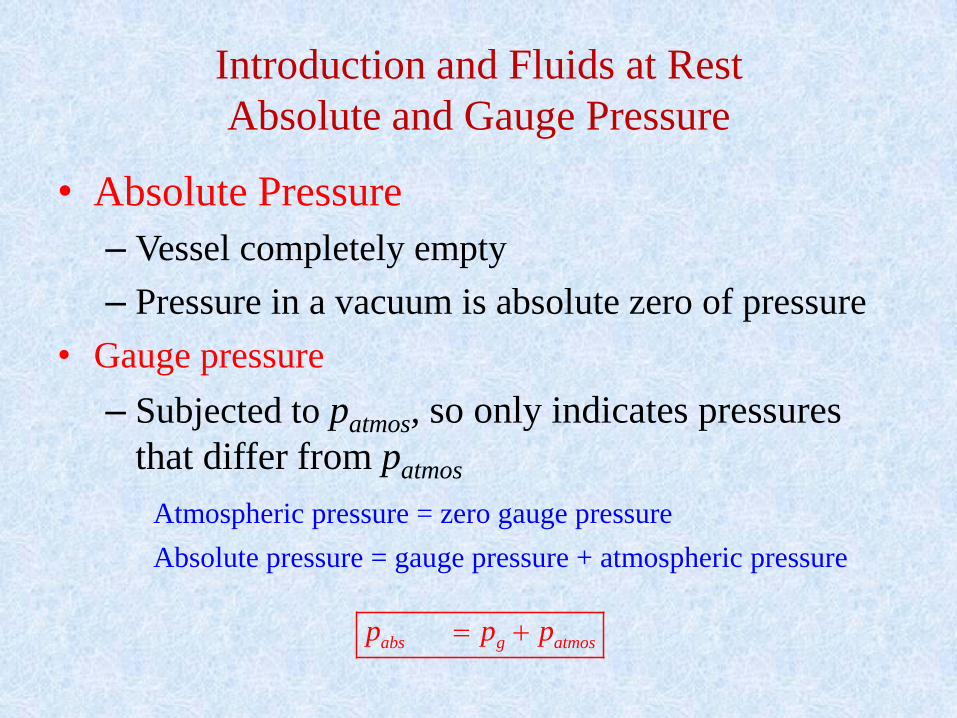
Absolute and Gauge Pressure
• Absolute Pressure
– Vessel completely empty
– Pressure in a vacuum is absolute zero of pressure
• Gauge pressure
– Subjected to patmos, so only indicates pressures
that differ from patmos
Atmospheric pressure = zero gauge pressure
Absolute pressure = gauge pressure + atmospheric pressure
abs g atmosp p p
Introduction and Fluids at Rest
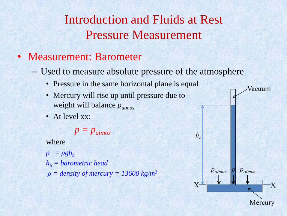
Pressure Measurement
• Measurement: Barometer
– Used to measure absolute pressure of the atmosphere
• Pressure in the same horizontal plane is equal
• Mercury will rise up until pressure due to
weight will balance patmos
• At level xx:
p = patmos
where
p = ρghb
hb = barometric head
ρ = density of mercury = 13600 kg/m3
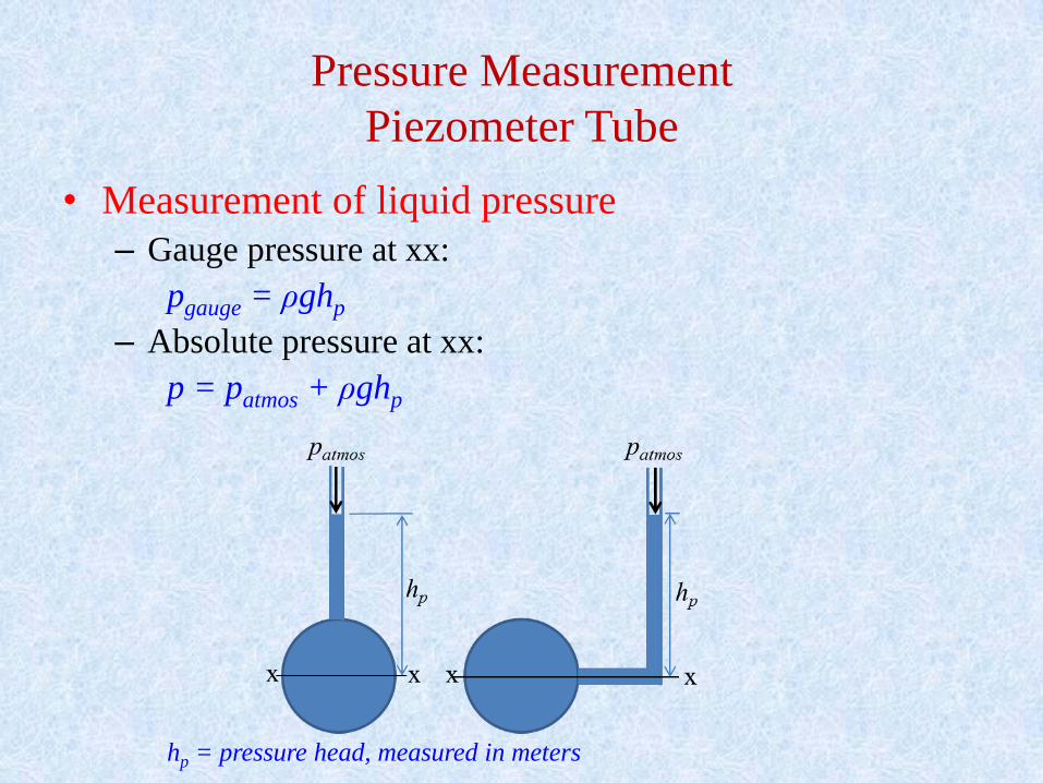
Pressure Measurement
Piezometer Tube
• Measurement of liquid pressure
– Gauge pressure at xx:
pgauge = ρghp
– Absolute pressure at xx:
p = patmos + ρghp
hp = pressure head, measured in meters
Pressure Measurement
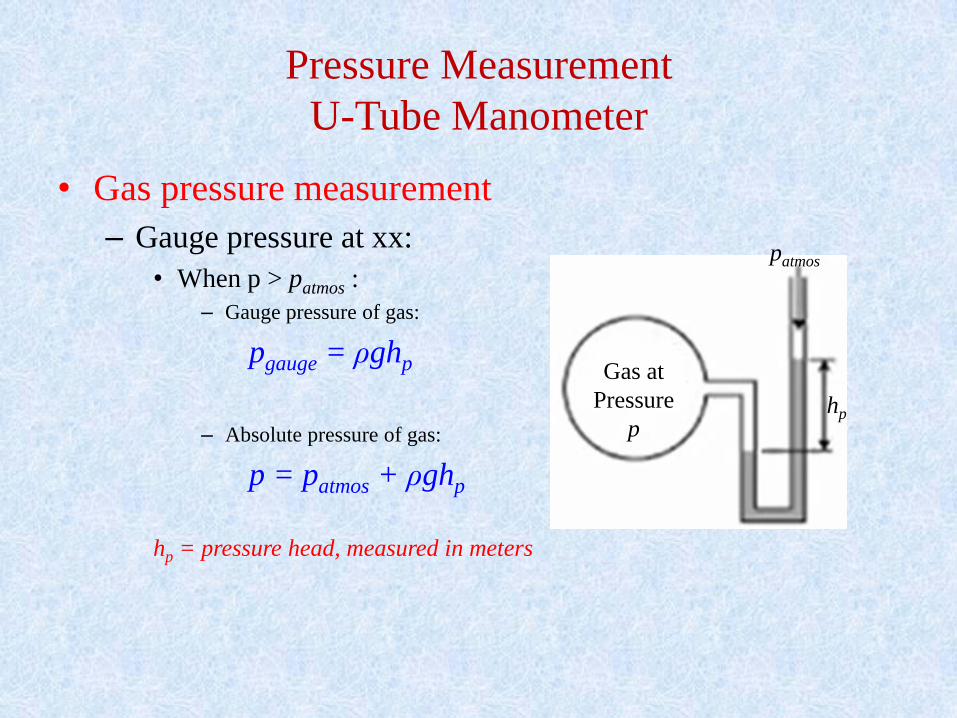
U-Tube Manometer
• Gas pressure measurement
– Gauge pressure at xx:
• When p > patmos :
– Gauge pressure of gas:
pgauge = ρghp
– Absolute pressure of gas:
p = patmos + ρghp
hp = pressure head, measured in meters
Gas at
Pressure
p
patmos
hp
Pressure Measurement
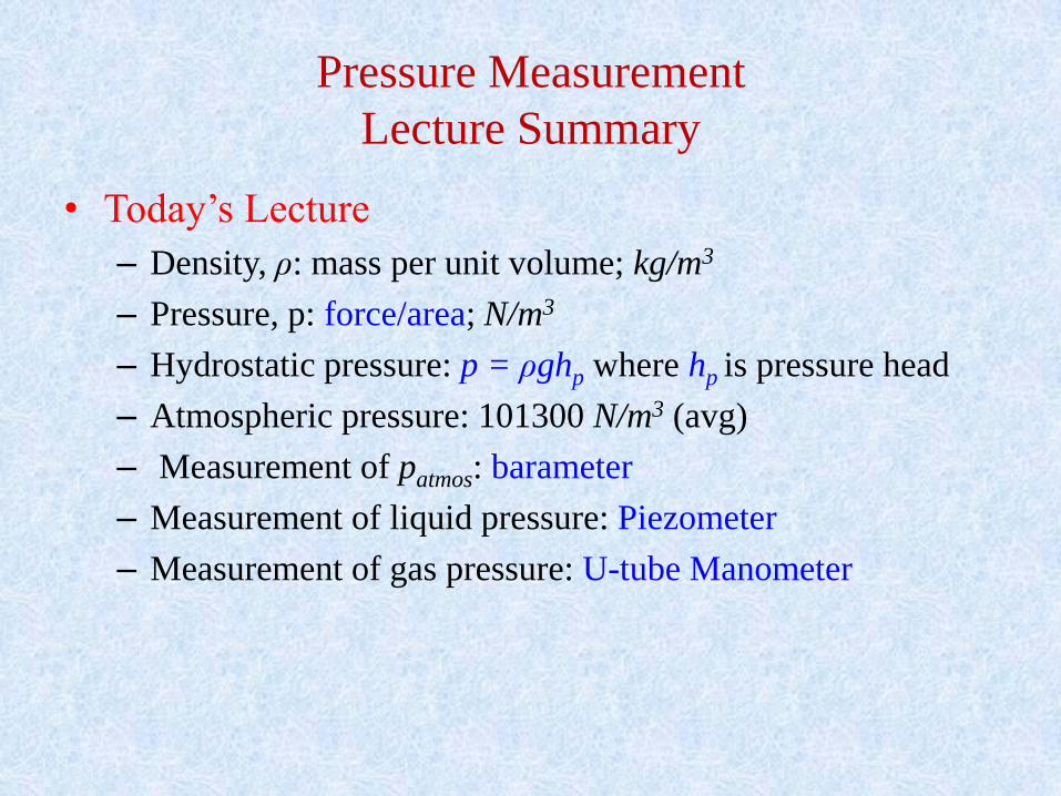
Lecture Summary
• Today’s Lecture
– Density, ρ: mass per unit volume; kg/m3
– Pressure, p: force/area; N/m3
– Hydrostatic pressure: p = ρghp where hp is pressure head
– Atmospheric pressure: 101300 N/m3 (avg)
– Measurement of patmos: barameter
– Measurement of liquid pressure: Piezometer
– Measurement of gas pressure: U-tube Manometer
Course Content
1. Fluid Properties Overview
2. Flow in Horizontal Pipeline o Liquid Phase
o Gas Phase
o Multiphase
Dr. Almarri
Eng. Aldousari
Petroleum Transportation & Storage
Engineering 124
• Oil and gas properties are very important in the pipeline
flow calculations
• API, Oil specific gravity, and Oil formation volume factor
• Gas density, gas formation volume factor, and gas specific
gravity.
Dr. Almarri
Eng. Aldousari
Petroleum Transportation & Storage
Engineering 125
Fluid Properties Overview
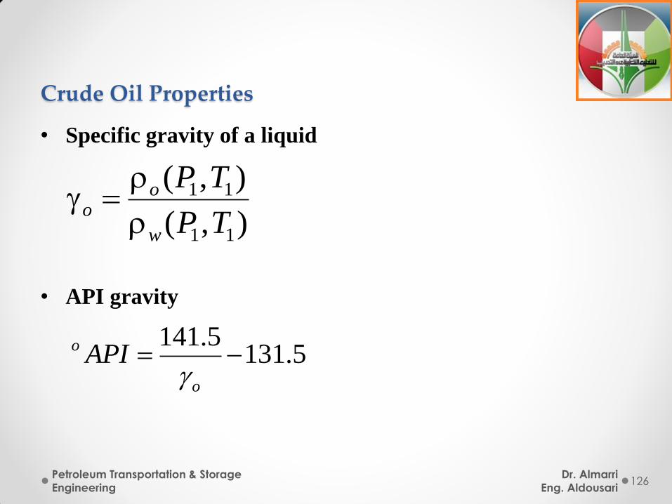
• Specific gravity of a liquid
• API gravity
Dr. Almarri
Eng. Aldousari
Petroleum Transportation & Storage
Engineering 126
),(
),(
11
11
TP
TP
w
oo
141.5131.5o
o
API
Crude Oil Properties
• Phase density (gas)
Dr. Almarri
Eng. Aldousari
Petroleum Transportation & Storage
Engineering 127
g
g
g
g
g
g
g
g
g g g g
g
g g
m
V
PVZ
n RT
mn
M
PV M m PMZ
m RT V ZRT
Dr. Almarri
Eng. Aldousari
Petroleum Transportation & Storage
Engineering 128
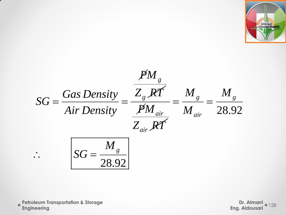
g
g
PM
Z RTGas DensitySG
Air Density
air
air
PM
Z RT
28.92
28.92
g g
air
g
M M
M
MSG
Dr. Almarri
Eng. Aldousari
Petroleum Transportation & Storage
Engineering 129
Pb
Oil
Vis
cosi
ty
T = constant
Single Phase Flow
Two Phase Flow
Gas Out of Solution
Gas formation volume factor Bg
Dr. Almarri
Eng. Aldousari
Petroleum Transportation & Storage
Engineering 130
Reservoir Conditions VR
Standard Conditions VSC
Dr. Almarri
Eng. Aldousari
Petroleum Transportation & Storage
Engineering 131
Rg
SC
VB
V
Bg=
Dr. Almarri
Eng. Aldousari
Petroleum Transportation & Storage
Engineering 132
[res bbl/SCF] or [ft3/SCF]
SC
SCSC
P
nRTZ
P
ZnRT
Bg
Dr. Almarri
Eng. Aldousari
Petroleum Transportation & Storage
Engineering 133
Since Tsc = 520 oR, Psc =14.696 psia, for all practical purposes Zsc = 1, then
14.6
ZT0.02
96
1 520
82P
scg o
sc sc sc sc sc sc
sc c
g
s
ZnRT ZnRTPZ T Z T psiaP PB
Z nRT Z nRT Z T P R P
cuftB
cf
P P
s
Oil Formation Volume Factor
Dr. Almarri
Eng. Aldousari
Petroleum Transportation & Storage
Engineering 134
Volume of Oil + Dissolved gas at Reservoir Pressure & Temperature
Volume of Oil entering Stoc
Reservoir barrels (bbl)
Stock tank barrels (
k tank at Standard Pressure & Temper
STB)
ature o
Units
B
1. Introduction
• We will talk about the transport of fluids from the
wellhead to the facility where processing of the fluids
begins.
• For oil production:
The facility is typically a two or three phase separator.
• For gas production:
The facility is a gas plant which is a compressor
station or a transport pipeline.
Dr. Almarri
Eng. Aldousari
Petroleum Transportation & Storage
Engineering 135
2. Flow in Horizontal Pipeline
• We will study the flow in horizontal pipes for gas, liquid,
and multiphase.
• Our main objective is to predict the pressure drop due to
friction.
• The pressure drop due to potential energy is zero in
horizontal pipelines.
Dr. Almarri
Eng. Aldousari
Petroleum Transportation & Storage
Engineering 136
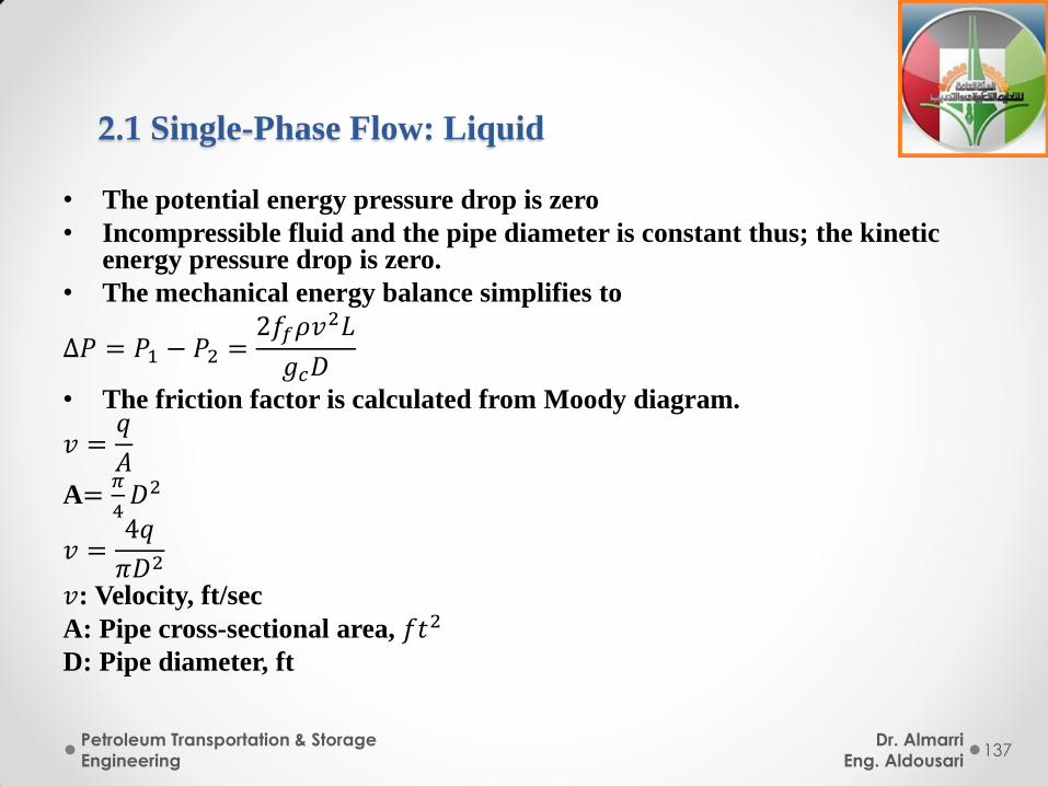
2.1 Single-Phase Flow: Liquid
• The potential energy pressure drop is zero
• Incompressible fluid and the pipe diameter is constant thus; the kinetic energy pressure drop is zero.
• The mechanical energy balance simplifies to
∆𝑃 = 𝑃1 − 𝑃2 =2𝑓𝑓𝜌𝑣
2𝐿
𝑔𝑐𝐷
• The friction factor is calculated from Moody diagram.
𝑣 =𝑞
𝐴
A=𝜋
4𝐷2
𝑣 =4𝑞
𝜋𝐷2
𝑣: Velocity, ft/sec
A: Pipe cross-sectional area, 𝑓𝑡2
D: Pipe diameter, ft
Dr. Almarri
Eng. Aldousari
Petroleum Transportation & Storage
Engineering 137
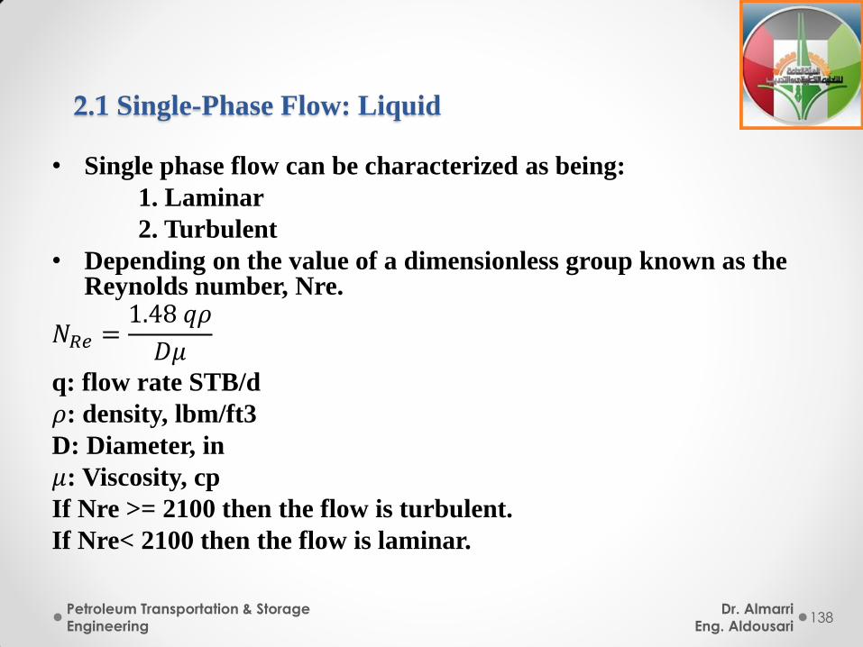
• Single phase flow can be characterized as being:
1. Laminar
2. Turbulent
• Depending on the value of a dimensionless group known as the Reynolds number, Nre.
𝑁𝑅𝑒 =1.48 𝑞𝜌
𝐷𝜇
q: flow rate STB/d
𝜌: density, lbm/ft3
D: Diameter, in
𝜇: Viscosity, cp
If Nre >= 2100 then the flow is turbulent.
If Nre< 2100 then the flow is laminar.
2.1 Single-Phase Flow: Liquid
Dr. Almarri
Eng. Aldousari
Petroleum Transportation & Storage
Engineering 138
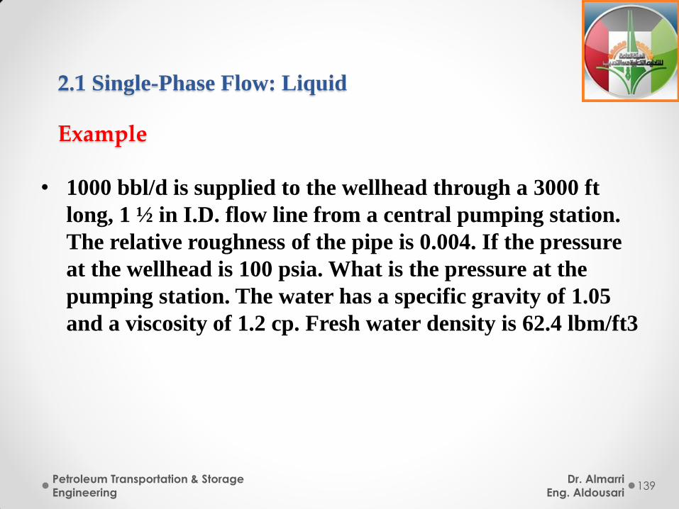
Example
• 1000 bbl/d is supplied to the wellhead through a 3000 ft
long, 1 ½ in I.D. flow line from a central pumping station.
The relative roughness of the pipe is 0.004. If the pressure
at the wellhead is 100 psia. What is the pressure at the
pumping station. The water has a specific gravity of 1.05
and a viscosity of 1.2 cp. Fresh water density is 62.4 lbm/ft3
2.1 Single-Phase Flow: Liquid
Dr. Almarri
Eng. Aldousari
Petroleum Transportation & Storage
Engineering 139
Solution
• Solution
2 3
3
2 2 2
1000 3000 1.5 0.004
100 1.05 1.2 62.4
1.05 62.4 65.52
3.142861.5
4 4
fw
fw
bblq L ft D in
d
lbmP psia cp
ft
lbm
ft
SOLUTI
A D in
ON
m
2
2
1
144
ft
in 20.01227
1000
ft
bbl
qV
A
d
35.615 ft
2
1bbl
1d
2
24 60 60
0.01227
s
ft
5.298
ft
s
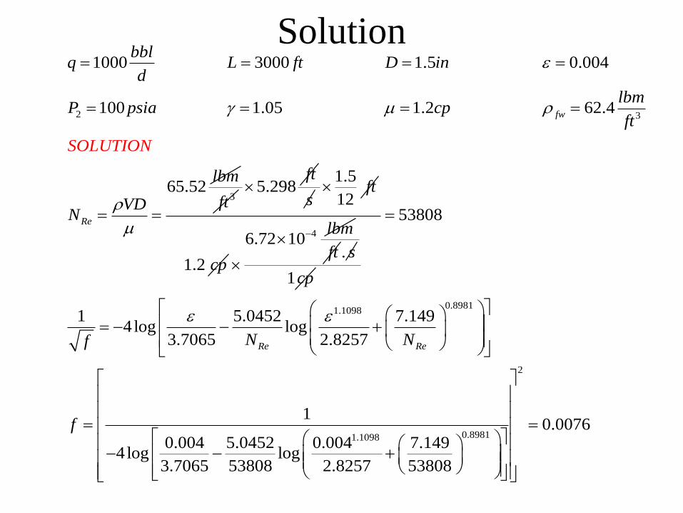
Solution
2 3
1000 3000 1.5 0.004
100 1.05 1.2 62.4
65.52
fw
Re
bblq L ft D in
d
l
SOLUTION
bmP psia cp
ft
lbm
VDN
m
m
3ft5.298
ft
s
1.5
12ft
1.2 cp
46.72 10lbm
ft . s
1cp
0.89811.1098
2
0.89811.1098
53808
1 5.0452 7.1494log log
3.7065 2.8257
10.0076
0.004 5.0452 0.004 7.1494log log
3.7065 53808 2.8257 53808
Re ReN Nf
f
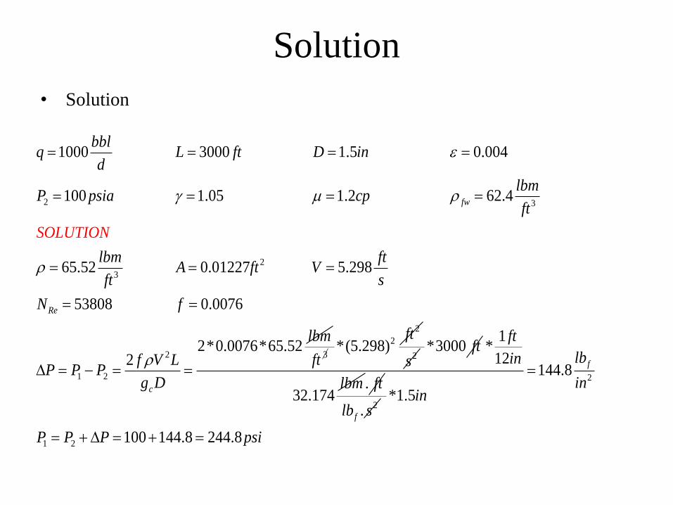
Solution
• Solution
2 3
2
3
2
1 2
1000 3000 1.5 0.004
100 1.05 1.2 62.4
65.52 0.01227 5.298
53808 0.0076
2*0.0076*65.522
fw
Re
c
bblq L ft D in
d
lbmP psia cp
ft
lbm ftA f
SOLU
t Vft s
N f
lbm
f V LP P P
TION
g D
m
3ft
2
2*(5.298)ft
2s*3000 ft
1*
12
32.174
ft
in
lbm . ft
2.flb s
2
1 2
144.8
*1.5
100 144.8 244.8
flb
inin
P P P psi
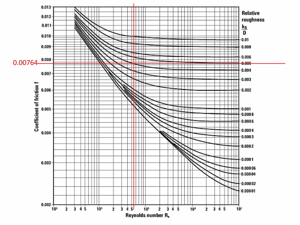
0.00764
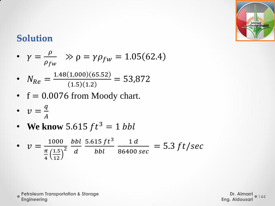
Solution
• 𝛾 =𝜌
𝜌𝑓𝑤 ≫ ρ = 𝛾𝜌𝑓𝑤 = 1.05 62.4
• 𝑁𝑅𝑒 =1.48 1,000 65.52
1.5 1.2= 53,872
• f = 0.0076 from Moody chart.
• 𝑣 =𝑞
𝐴
• We know 5.615 𝑓𝑡3 = 1 𝑏𝑏𝑙
• 𝑣 =1000
𝜋
4
1.5
12
2 𝑏𝑏𝑙
𝑑 5.615 𝑓𝑡3
𝑏𝑏𝑙
1 𝑑
86400 𝑠𝑒𝑐 = 5.3 𝑓𝑡/𝑠𝑒𝑐
Dr. Almarri
Eng. Aldousari
Petroleum Transportation & Storage
Engineering 144

Lecture 3
Dr. Almarri
Eng. Aldousari 145
Petroleum Transportation & Storage
Engineering
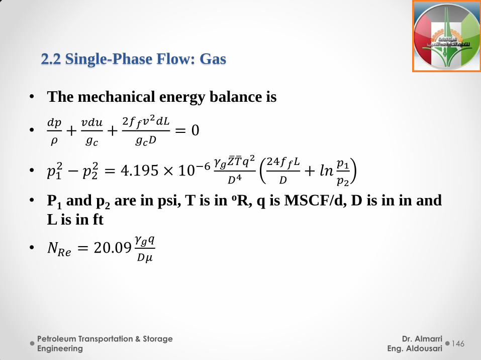
• The mechanical energy balance is
•𝑑𝑝
𝜌+
𝑣𝑑𝑢
𝑔𝑐+
2𝑓𝑓𝑣2𝑑𝐿
𝑔𝑐𝐷= 0
• 𝑝12 − 𝑝2
2 = 4.195 × 10⁻⁶ 𝛾𝑔𝑍 𝑇 𝑞2
𝐷4
24𝑓𝑓𝐿
𝐷+ 𝑙𝑛
𝑝1
𝑝2
• P1 and p2 are in psi, T is in oR, q is MSCF/d, D is in in and
L is in ft
• 𝑁𝑅𝑒 = 20.09𝛾𝑔𝑞
𝐷𝜇
2.2 Single-Phase Flow: Gas
Dr. Almarri
Eng. Aldousari
Petroleum Transportation & Storage
Engineering 146
Example
• Gas production from a low-pressure gas well (wellhead
pressure = 100 psia) is to be transported through 1,000 ft of
a 3 in. I.D. (Ԑ= 0.001) to a compressor station, ehre the inlet
pressure must be at least 20 psia. The gas has a specific
gravity of 0.7, a temperature of 100 oF and an average
viscosity of 0.012 cp. What is the maximum flow rate
possible through this gas line? (Hint: when the pressure is
low z= 1). Final answer = 10,800 MSCF/d
2.2 Single-Phase Flow: Gas
Dr. Almarri
Eng. Aldousari
Petroleum Transportation & Storage
Engineering 147
Solution
• Solution
1 2
2 2 2
100 1000 3 0.001
100 20 0.7 0.012
3.142863
4 4
o
g
T F L ft D in
P psia P psia c
SOL
p
A D in
UTION
m
2
2
1
144
ft
in 2
Re
0.04911
500
0.7*1000020.09 20.09 195319.4
3*0.012
g
ft
MSCFAssume q
d
qN
D
m
Solution
1 2
2
Re
0.89811.1098
100 1000 3 0.001 1
100 20 0.7 0.012
0.04911 500 195319.4
1
5.0452 7.1494log log
3.7065 2.8257
o
g
Re Re
T F L ft D in Z
P psia P psia cp
MSCFA ft Assume q N
SOLUTION
d
f
N N
m
2
2
0.89811.1098
10.00527761
0.001 5.0452 0.001 7.1494log log
3.7065 195319.4 2.8257 195319.4
f
Solution
• Solution
1 2
2
Re
2 2 4
1 2
7
100 1000 3 0.001 1
100 20 0.7 0.012
0.04911 500 195319.4 0.00527761
(4.195 10 ) 24
o
g
g
T F L ft D in Z
P psia P psia cp
MSCFA ft Assume q N f
d
q is calculated again by the following :
P P Dq
LZT f
D
SOLUTION
m
1
2
2 2 4
7
ln
100 20 310386.80102
1000 100(4.195 10 ) 0.7 1 (460 100) 24 0.00528 ln
3 20
P
P
q
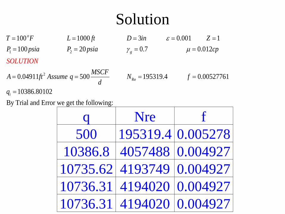
Solution
1 2
2
Re
100 1000 3 0.001 1
100 20 0.7 0.012
0.04911 500 195319.4 0.00527761
10386.80102
By Trial and Error we get the following:
o
g
i
T F L ft D in Z
P psia P psia cp
MSCFA ft Assume
SOL
q N f
UTION
d
q
m
q Nre f
500 195319.4 0.005278
10386.8 4057488 0.004927
10735.62 4193749 0.004927
10736.31 4194020 0.004927
10736.31 4194020 0.004927

2.3 Two Phase Flow
Flow Regimes
• Flow regime does not affect the pressure drop as
significantly in horizontal flow as it does in vertical flow,
because there is no potential energy contribution.
• Most important, the occurance of slug flow nesessitates
designing separators or sometimes special pieces of
equipment. (Slug catchers) to handle the large volume of
liquid containes in a slug.
Dr. Almarri
Eng. Aldousari
Petroleum Transportation & Storage
Engineering 153
• Segregated flow: two phases are separate
• Intermittent flow: gas and liquid are alternating.
• Distibutive flow: one phase is dispersed in the other
Dr. Almarri
Eng. Aldousari
Petroleum Transportation & Storage
Engineering 154
Segregated flow
• Stratified smooth flow: consists of liquid flowing along the
bottom of the pipe and gas flowing along the top of the
pipe with smooth interface between the phases, occires at
tye low rates od both phases.
• At higher gas rates, the interface becomes wavy, and
stratified wavy flow results.
Dr. Almarri
Eng. Aldousari
Petroleum Transportation & Storage
Engineering 155
• Annular flow: occurs at high gas rates and relativley high
liquid rates and consists of an annulus of liquid coating the
wall of the pipe and a central core of gas flow, with liquid
droplets entrained in the gas.
Dr. Almarri
Eng. Aldousari
Petroleum Transportation & Storage
Engineering 156
Intermittent flow
• Slug flow: consists of large liquid slugs alternating with
high velocity bubbles of gas that fill almost the entire pipe.
• Plug flow: large gas bubbles flow along the top of the pipe.
Dr. Almarri
Eng. Aldousari
Petroleum Transportation & Storage
Engineering 157
Distributive flow
• Bubble flow: gas bubble concentrated on the upper side of
the pipe.
• Mist flow: occurs at high gas rates and low liquid rates and
consists of gas with liquid droplets entrained.
Dr. Almarri
Eng. Aldousari
Petroleum Transportation & Storage
Engineering 158
Determination of flow type
• Flow regime in horizontal flow are predicted with flow
regime maps one of the first of these is Baker (1953). We
will study
• 1- Baker (1953)
• 2- Mandhane (1974)
• Beggs and Brill (1973)
Dr. Almarri
Eng. Aldousari
Petroleum Transportation & Storage
Engineering 159
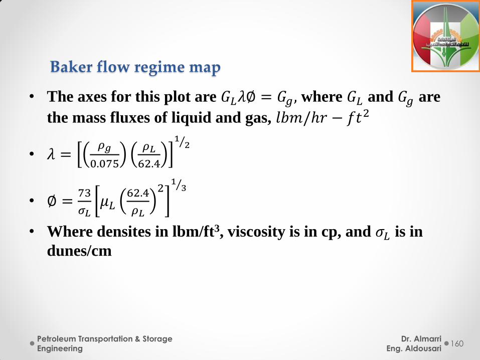
Baker flow regime map
• The axes for this plot are 𝐺𝐿𝜆∅ = 𝐺𝑔, where 𝐺𝐿 and 𝐺𝑔 are
the mass fluxes of liquid and gas, 𝑙𝑏𝑚/ℎ𝑟 − 𝑓𝑡2
• 𝜆 =𝜌𝑔
0.075
𝜌𝐿
62.4
12
• ∅ =73
𝜎𝐿𝜇𝐿
62.4
𝜌𝐿
21
3
• Where densites in lbm/ft3, viscosity is in cp, and 𝜎𝐿 is in
dunes/cm
Dr. Almarri
Eng. Aldousari
Petroleum Transportation & Storage
Engineering 160
Mandhane flow regime map
• This map uses the gas and liquid superficial velocities.
Dr. Almarri
Eng. Aldousari
Petroleum Transportation & Storage
Engineering 161
• The superficial velocity of a phase would be the average
velocity of the phase if that phase filled the entire pipe;
that is, if it were single phase flow. It is not a real velocity
that physically occurs.
• 𝑣𝑠𝐿 =𝑞𝐿
𝐴
• 𝑣𝑠𝑔 =𝑞𝐿𝑔
𝐴
Dr. Almarri
Eng. Aldousari
Petroleum Transportation & Storage
Engineering 162
• The Begges and Brill Correlation
• Is based on a horizontal flow regime map that divides the
domain into the tree flow regime categories, segregated,
intermittent, and distributed. This map needs mixture
Froud number as
• 𝑁𝑓𝑟 =𝑣𝑚2
𝑔𝐷
• Vm: vsl + vsg
• Vm: mixture velocity, ft/s
• g: gravity constant 32.17 ft/sec2
• D: diameter, ft
Dr. Almarri
Eng. Aldousari
Petroleum Transportation & Storage
Engineering 163
• Example
• Using the baker, Mandhane, and Beggs and Brill flow
regime maps, determine the flow regime for the flow of
2000 bbl/d of oil and 1 MM SCF/d of gas at 800 psia and
175 oF in a 2.5 in I.D. pipe. 𝜌𝑜= 0.8 g/cm3, 𝜇𝑜= 2 cp, 𝜎𝐿= 30
dynes/cm
• 1 g/cc = 62.428 lbm/ft3, Tpc= 374 oR, Ppc= 717 psia, 𝛾𝑔=
0.709, 𝜇𝑜= 0.0131 cp
Dr. Almarri
Eng. Aldousari
Petroleum Transportation & Storage
Engineering 164
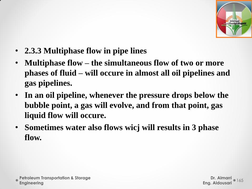
• 2.3.3 Multiphase flow in pipe lines
• Multiphase flow – the simultaneous flow of two or more
phases of fluid – will occure in almost all oil pipelines and
gas pipelines.
• In an oil pipeline, whenever the pressure drops below the
bubble point, a gas will evolve, and from that point, gas
liquid flow will occure.
• Sometimes water also flows wicj will results in 3 phase
flow.
Dr. Almarri
Eng. Aldousari
Petroleum Transportation & Storage
Engineering 165
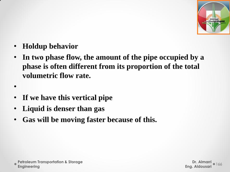
• Holdup behavior
• In two phase flow, the amount of the pipe occupied by a
phase is often different from its proportion of the total
volumetric flow rate.
•
• If we have this vertical pipe
• Liquid is denser than gas
• Gas will be moving faster because of this.
Dr. Almarri
Eng. Aldousari
Petroleum Transportation & Storage
Engineering 166
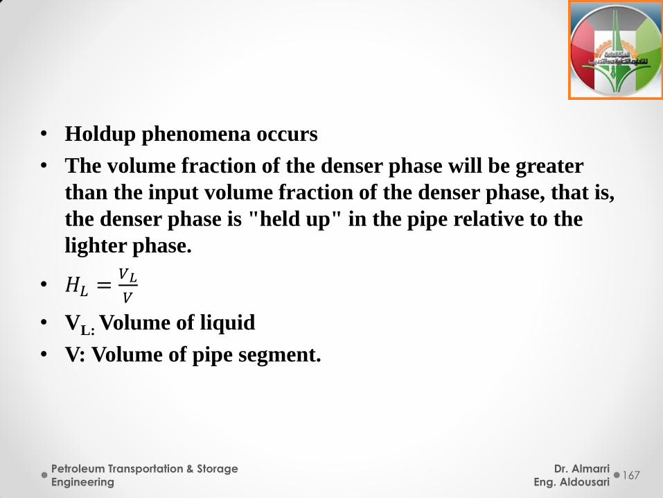
• Holdup phenomena occurs
• The volume fraction of the denser phase will be greater
than the input volume fraction of the denser phase, that is,
the denser phase is "held up" in the pipe relative to the
lighter phase.
• 𝐻𝐿 =𝑉𝐿
𝑉
• VL: Volume of liquid
• V: Volume of pipe segment.
Dr. Almarri
Eng. Aldousari
Petroleum Transportation & Storage
Engineering 167
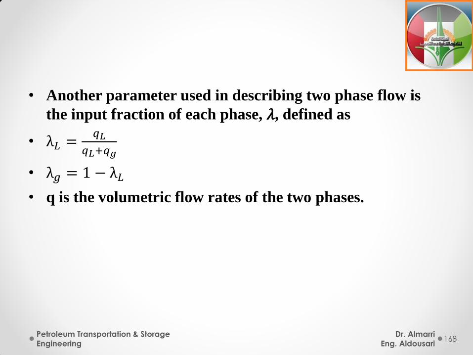
• Another parameter used in describing two phase flow is
the input fraction of each phase, 𝜆, defined as
• λ𝐿 =𝑞𝐿
𝑞𝐿+𝑞𝑔
• λ𝑔 = 1 − λ𝐿
• q is the volumetric flow rates of the two phases.
Dr. Almarri
Eng. Aldousari
Petroleum Transportation & Storage
Engineering 168
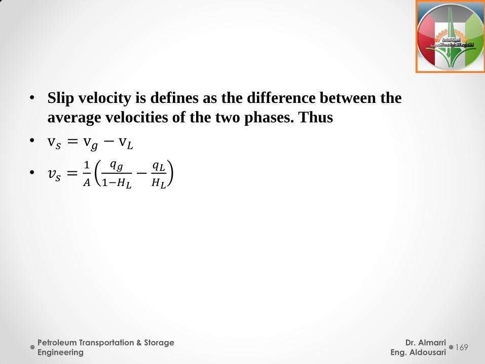
• Slip velocity is defines as the difference between the
average velocities of the two phases. Thus
• v𝑠 = v𝑔 − v𝐿
• 𝑣𝑠 =1
𝐴
𝑞𝑔
1−𝐻𝐿−
𝑞𝐿
𝐻𝐿
Dr. Almarri
Eng. Aldousari
Petroleum Transportation & Storage
Engineering 169
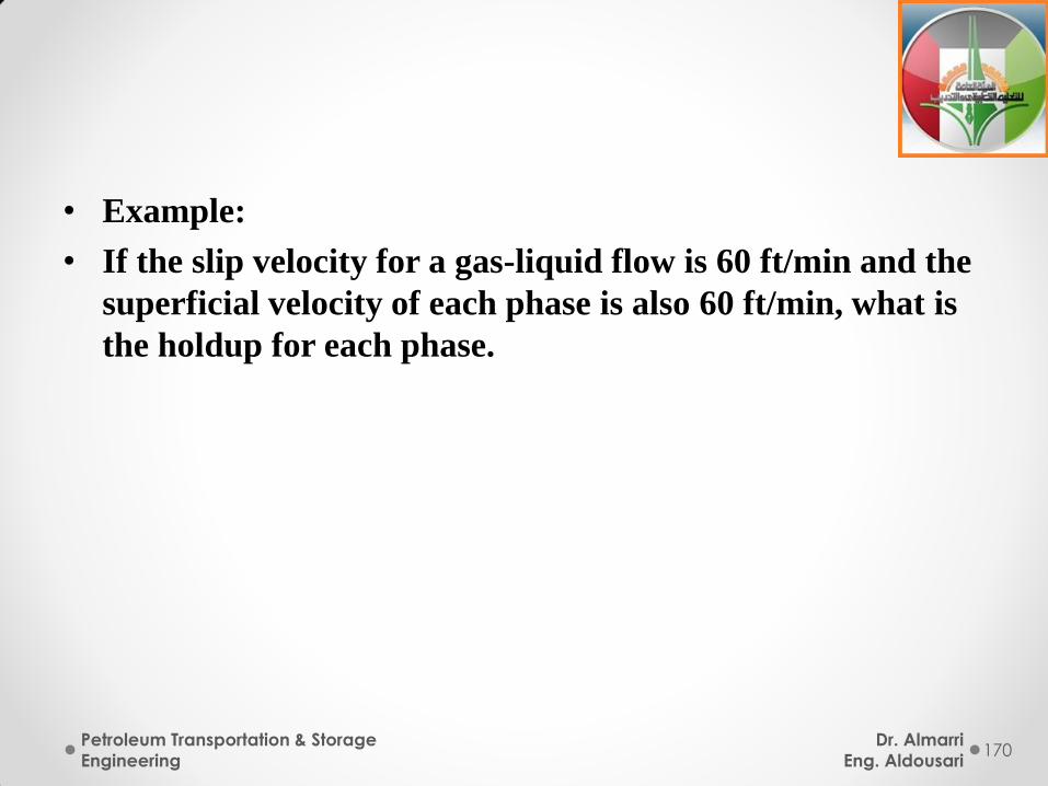
• Example:
• If the slip velocity for a gas-liquid flow is 60 ft/min and the
superficial velocity of each phase is also 60 ft/min, what is
the holdup for each phase.
Dr. Almarri
Eng. Aldousari
Petroleum Transportation & Storage
Engineering 170
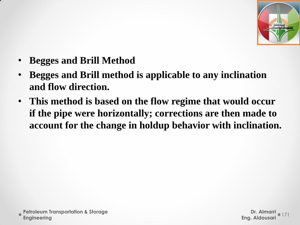
• Begges and Brill Method
• Begges and Brill method is applicable to any inclination
and flow direction.
• This method is based on the flow regime that would occur
if the pipe were horizontally; corrections are then made to
account for the change in holdup behavior with inclination.
Dr. Almarri
Eng. Aldousari
Petroleum Transportation & Storage
Engineering 171
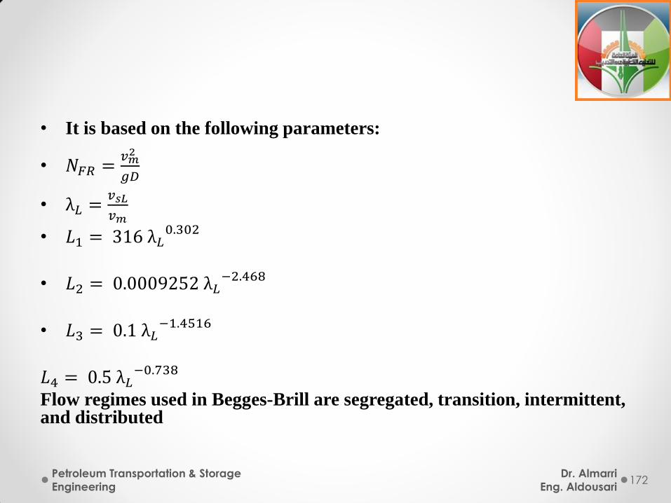
• It is based on the following parameters:
• 𝑁𝐹𝑅 =𝑣𝑚2
𝑔𝐷
• λ𝐿 =𝑣𝑠𝐿
𝑣𝑚
• 𝐿1 = 316 λ𝐿0.302
• 𝐿2 = 0.0009252 λ𝐿−2.468
• 𝐿3 = 0.1 λ𝐿−1.4516
𝐿4 = 0.5 λ𝐿−0.738
Flow regimes used in Begges-Brill are segregated, transition, intermittent, and distributed
Dr. Almarri
Eng. Aldousari
Petroleum Transportation & Storage
Engineering 172
Flow through chokes
• The flow rate from almost all flowing wells is controlled
with a wellhead choke
• The chock is a device that places a restriction in the flow
line.
• Chock advantages:
• Prevention of water conning
• Prevention of sand production
• Satisfying production rate or pressure imposed by surface
equipment.
Dr. Almarri
Eng. Aldousari
Petroleum Transportation & Storage
Engineering 173
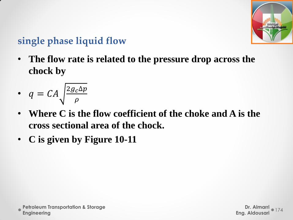
single phase liquid flow
• The flow rate is related to the pressure drop across the
chock by
• 𝑞 = 𝐶𝐴2𝑔𝑐∆𝑝
𝜌
• Where C is the flow coefficient of the choke and A is the
cross sectional area of the chock.
• C is given by Figure 10-11
Dr. Almarri
Eng. Aldousari
Petroleum Transportation & Storage
Engineering 174
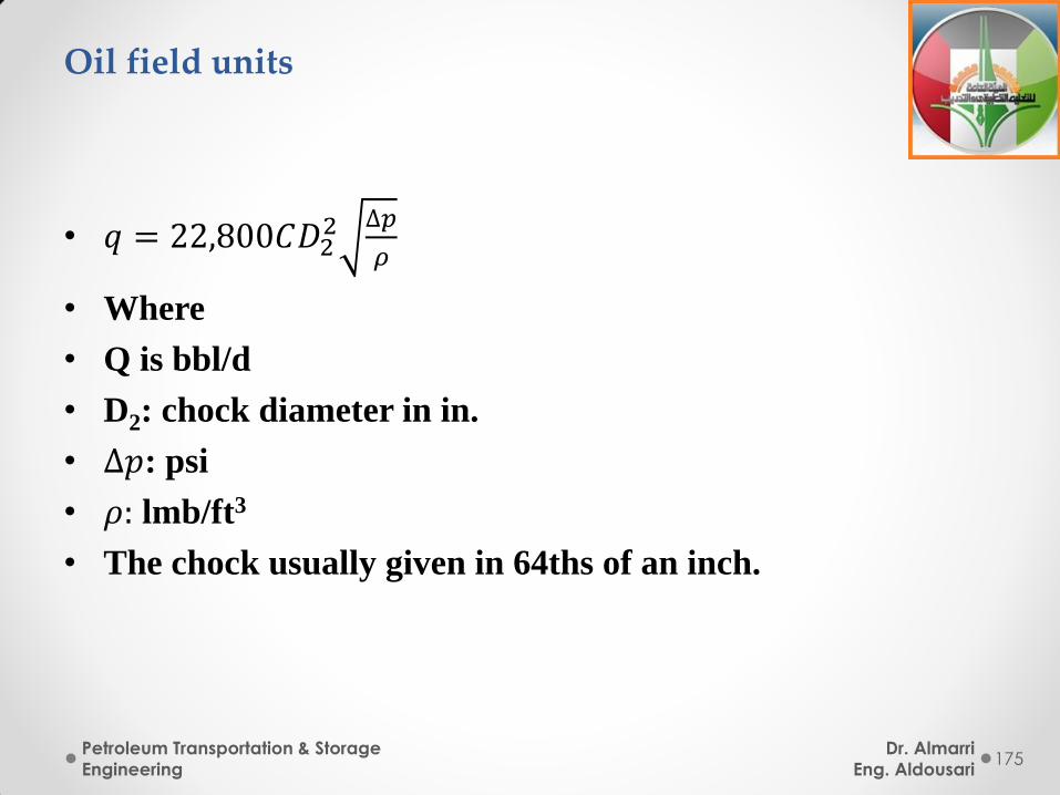
Oil field units
• 𝑞 = 22,800𝐶𝐷22 ∆𝑝
𝜌
• Where
• Q is bbl/d
• D2: chock diameter in in.
• ∆𝑝: psi
• 𝜌: lmb/ft3
• The chock usually given in 64ths of an inch.
Dr. Almarri
Eng. Aldousari
Petroleum Transportation & Storage
Engineering 175
Example
• What will be the flow rate of a 0.8 specific gracity, 2 cp oil
through a 20/64-in chock if the pressure drop across the
chock is 20 psi and the line size is 1 in.
Dr. Almarri
Eng. Aldousari
Petroleum Transportation & Storage
Engineering 176
Pressure drop through pipe fittings
• When fluids pass through pipe fittings (tees, elbows, etc) or valves, secondary flows and additional turbulence create pressure drops that must be included to determine the overall pressure drop in a piping network.
• The effects of valves and fittings are included by adding the "equivalent length" of the valves and fittings to the actual lengths of straight pipe whrn calculating the pressure drop.
• The equivalent lengths of many standard valves and fittings have been determined experimentally (crane, 1957) and are given in Table 10-1
• The equivelant lengths are given in pipe diameters, this value is multiplied by the pipe diameter to find the actual length of pipe to be added.
Dr. Almarri
Eng. Aldousari
Petroleum Transportation & Storage
Engineering 177
Surface gathering systems
• In most oil and gas production installations, the flow from
several wells will be gathered at a central processing
station or combined into a common pipeline
• When individual flow lines all join at a common point, the
pressure at the common point is equal for all flow lines.
• The common point is typically a separator in an oil
production systems.
• The flowing tubing pressure of an individual well (i) is
related to the separator pressure by
Dr. Almarri
Eng. Aldousari
Petroleum Transportation & Storage
Engineering 178
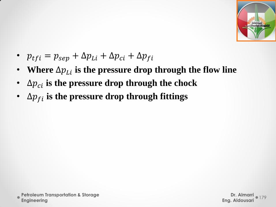
• 𝑝𝑡𝑓𝑖 = 𝑝𝑠𝑒𝑝 + ∆𝑝𝐿𝑖 + ∆𝑝𝑐𝑖 + ∆𝑝𝑓𝑖
• Where ∆𝑝𝐿𝑖 is the pressure drop through the flow line
• ∆𝑝𝑐𝑖 is the pressure drop through the chock
• ∆𝑝𝑓𝑖 is the pressure drop through fittings
Dr. Almarri
Eng. Aldousari
Petroleum Transportation & Storage
Engineering 179
• In a gathering system where individual wells are tied into a
common pipeline, so that pipeline flow rate is the sum of
the upstream well flow rates.
Dr. Almarri
Eng. Aldousari
Petroleum Transportation & Storage
Engineering 180
Example
• The liquid production from three rod-pimped wells is
gathered in a common 2 in line, as shown.
• 1 in flow lines connect each well to the gathering line, and
each well line contains a ball valve and a conventional
swing check valve. Well 1 is tied into the gathering line
with a standard 90o elbow, while wells 2 and 3 are
connected with standard tees.
• The oil density is 53.04 lbm/ft3 and its viscosity is 5 cp. The
separator pressure is 100 psig. Assuming the relative
roughness of all lines to be 0.001, calculate the flowing
tubing pressures of the three wells.
Dr. Almarri
Eng. Aldousari
Petroleum Transportation & Storage
Engineering 181
Drag Reducing Agents
• Drag reducing agnets (DRA) are added to crude oil to
allow a higher flow rate in a pipeline for the same pressure
drop.
•
• They are effective with light crude oil.
• DRA are expensive and not recoverable; their use must be
economically justified.
• DRA increases the flow up to 90%
• The effect of the DRA is to reduce the frictional pressure
drop in the turbulent flow; they reduce turbulence by an
unkown mechanism
Dr. Almarri
Eng. Aldousari
Petroleum Transportation & Storage
Engineering 182
Heavy oil Transport
• The viscosity of heavy oils is very high and highly sensitive
to the oil temperature.
• Dilute oil wil a light hydrocarbon solvent lowers the
viscosity to an acceptable value and allows pumping at
reasonable flow rates.
•
• Leak Detectiong
• Visual Surveilance
• Monitoring of flow and pressure.
Dr. Almarri
Eng. Aldousari
Petroleum Transportation & Storage
Engineering 183
• Pipe desiging
• Petroleum pipelines should not
• Exceed the maximum allowable working pressure
(MAWP)
• Fall below the crude oil bubble point pressure.
Dr. Almarri
Eng. Aldousari
Petroleum Transportation & Storage
Engineering 184
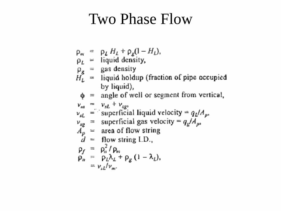
Two Phase Flow
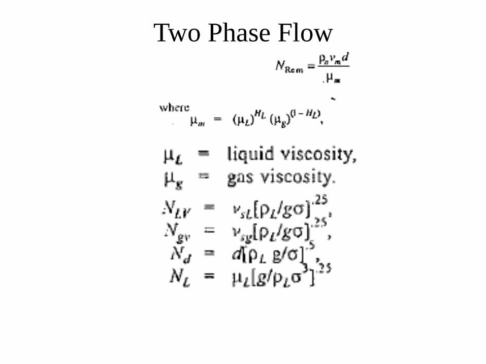
Two Phase Flow
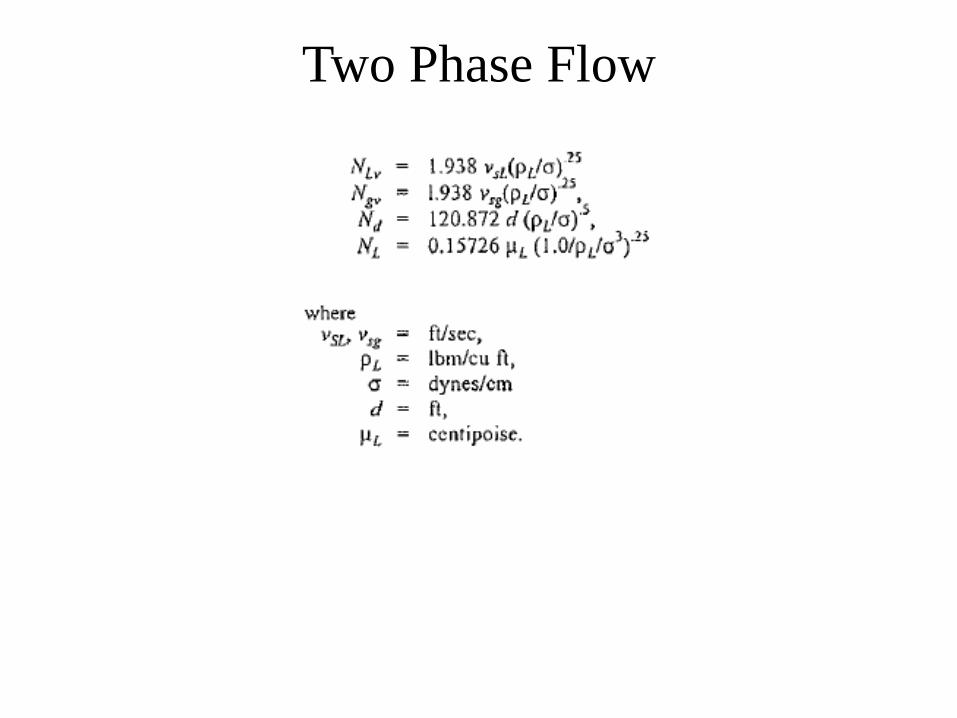
Two Phase Flow
Example
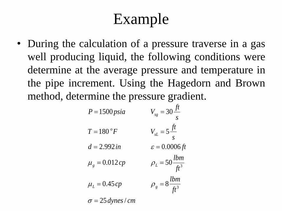
• During the calculation of a pressure traverse in a gas
well producing liquid, the following conditions were
determine at the average pressure and temperature in
the pipe increment. Using the Hagedorn and Brown
method, determine the pressure gradient.
3
3
1500 30
180 5
2.992 0.0006
0.012 50
0.45 8
25 /
sg
o
sL
g L
L g
ftP psia V
s
ftT F V
s
d in ft
lbmcp
ft
lbmcp
ft
dynes cm
m
m
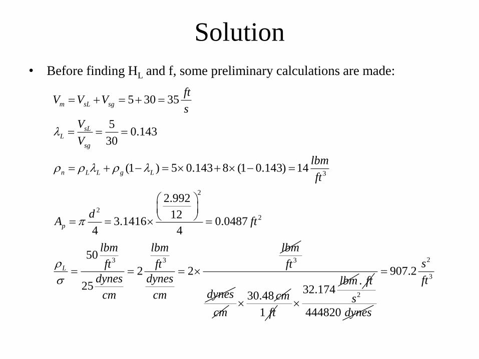
Solution
• Before finding HL and f, some preliminary calculations are made:
3
2
22
3 3
5 30 35
50.143
30
(1 ) 5 0.143 8 (1 0.143) 14
2.992
123.1416 0.0487
4 4
50
2 2
25
m sL sg
sLL
sg
n L L g L
p
L
ftV V V
s
V
V
lbm
ft
dA ft
lbm lbm lbm
ft ft
dynes dynes
cm cm
3ft
dynes
cm
30.48 cm
1 ft
32.174lbm
. ft2
444820
s
dynes
2
3907.2
s
ft
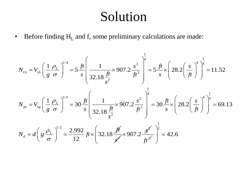
Solution
• Before finding HL and f, some preliminary calculations are made:
1
141/ 4 4 42
3
2
1
141/ 4 4 42
3
2
1 15 907.2 5 28.2 11.52
32.18
1 130 907.2 30 28.2 69.13
32.18
LLv sL
Lgv sg
d
ft s ft sN V
ftg s ft s ft
s
ft s ft sN V
ftg s ft s ft
s
N d
1/ 22.992
32.1812
Lft
g ft
2s
2
907.2s
3ft
2
1
2
42.6
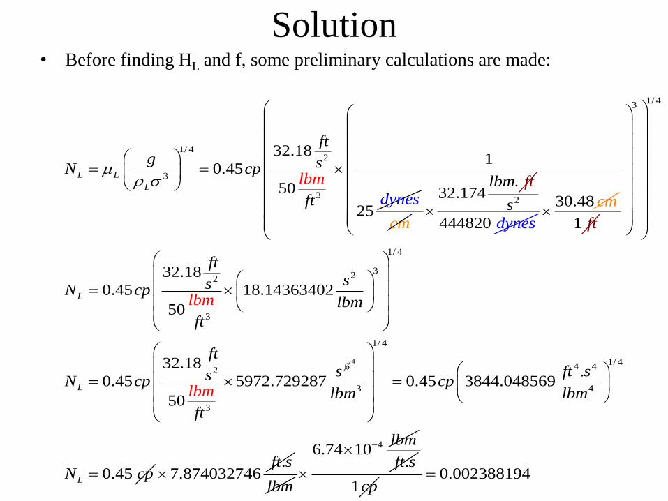
Solution • Before finding HL and f, some preliminary calculations are made:
1/ 42
3
3
32.181
0.45
50
25
L L
L
f
lbm
t
g sN cp
ft dynes
m
cm
.32.174
lbm ft
2
444820
s
dynes
30.48 cm
1 ft
1/ 43
1/ 4
322
3
62
3
32.18
0.45 18.14363402
50
32.18
0.45 5972.729287
50
L
L
ft
ssN cplbm
ft
ft
ssN cp
f
lbm
lb
t
m
4
1/ 4
1/ 44 4
3 4
.0.45 3844.048569
0.45L
ft scp
lbm lbm
N cp
.
7.874032746ft s
lbm
46.74 10lbm
.ft s
1cp0.002388194
Example
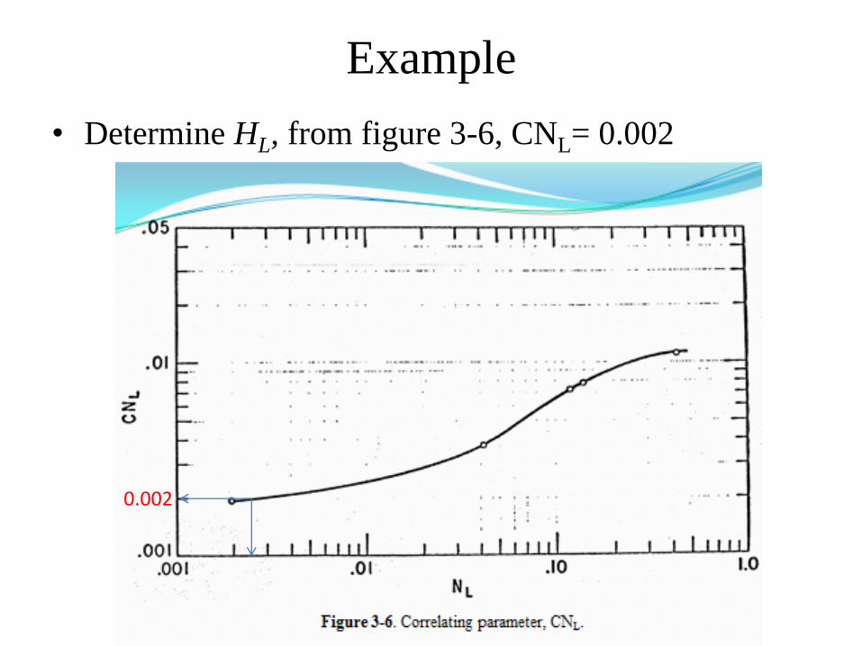
• Determine HL, from figure 3-6, CNL= 0.002
0.002
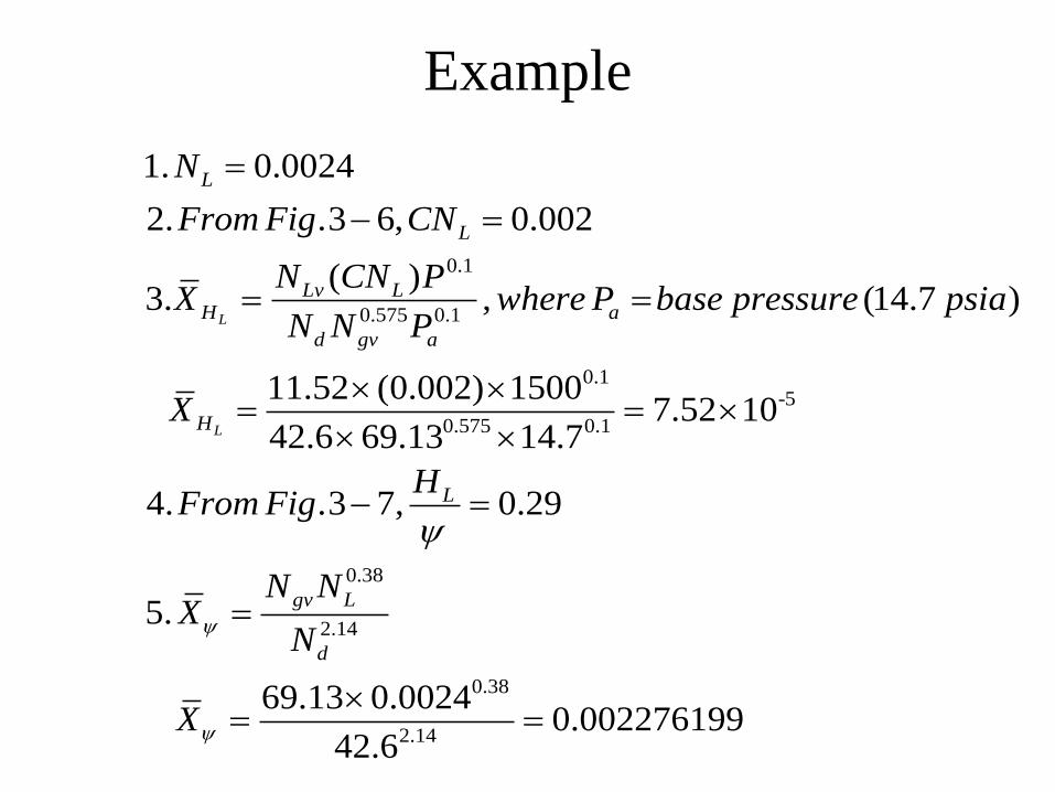
Example
0.1
0.575 0.1
0.1-5
0.575 0.1
0.38
2.14
1. 0.0024
2. .3 6, 0.002
( )3. , (14.7 )
11.52 (0.002) 15007.52 10
42.6 69.13 14.7
4. .3 7, 0.29
5.
L
L
L
L
Lv LH a
d gv a
H
L
gv L
d
N
From Fig CN
N CN PX where P base pressure psia
N N P
X
HFrom Fig
N NX
N
X
0.38
2.14
69.13 0.00240.002276199
42.6
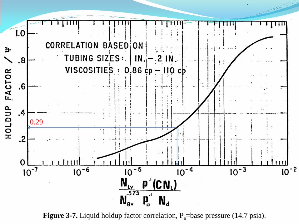
Figure 3-7. Liquid holdup factor correlation, Pa=base pressure (14.7 psia).
0.29
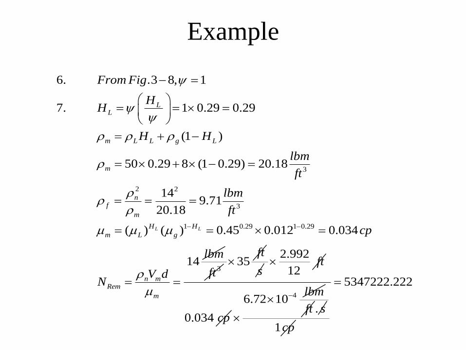
Example
3
2 2
3
1 0.29 1 0.29
6. .3 8, 1
7. 1 0.29 0.29
(1 )
50 0.29 8 (1 0.29) 20.18
149.71
20.18
( ) ( ) 0.45 0.012 0.034
14
L L
LL
m L L g L
m
nf
m
H H
m L g
n mRem
m
From Fig
HH
H H
lbm
ft
lbm
ft
cp
lbm
V dN
m m m
m
3ft35
ft
s
2.992
12ft
0.034 cp
46.72 10lbm
ft . s
1cp
5347222.222
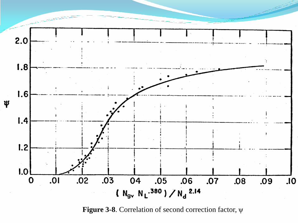
Figure 3-8. Correlation of second correction factor, ψ

Example
0.0006 ft
d
12 in
1 ft
2.992 in
0.9
Re
0.9
0.0024
.3 9 .3 15
0.025
1 21.251.14 2log
1 21.251.14 2 log 0.0024 6.373
5347222.2
0.157 0.024622659
m
from fig or Eq
f
d Nf
f
f f
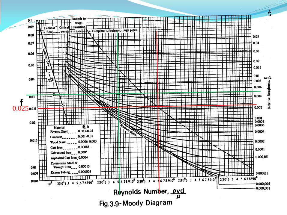
0.025
Example
2
( cos )2
32.2
f m
m
c c
f VdP g
dh g g d
ft
dP
dh
2s
32.174lbm . ft
2.flb s
20.18lbm
3
0.025 9.71
cos(0)
lbm
ft
2
2
335
ft
ft
2s
2 32.174lbm
. ft
2.flb s0.249 ft
3 220.19630758 18.55927159 38.75 38.75
f flb lbdP
dh ft ft
211 ft
ft
2
2
144
10.269 0.269
f
in
lbdP psi
dh in ft ft

200
APPENDIX A
CONVERSION FACTORS
Thermodynamics
201
APPENDIX A: CONVERSION FACTORS Mass 1.0 Kg Mass 1.0 lbm
= 1000.0 g = 16.0 oz
= 0.0010 metric ton = 0.00050 ton
= 2.20462 lbm = 453.59300 g
= 35.27392 oz = 0.45359 Kg
Length 1.0 m Length 1.0 ft
= 100.0 cm = 12.0 in
= 1000.0 mm = 1/3 yd
= 1000000.0 microns meter = 0.3048 m
= 10000000000.0 angstroms = 30.4800 cm
= 39.370 in
= 3.280800 ft
= 1.093600 yd
= 0.000621 mile
Volume 1 m3 Volume 1 ft3
= 1000 liters = 1728 in3
= 1000000 cm3 = 7.4805 gal
= 1000000 mlt = 0.028317 m3
= 35.3145 ft3 = 28.317 liters
= 220.83 imperial gallons = 28317 cm3
= 264.17 gal = 0.1781076 bbl
= 6.2898106 bbl
= 1056.68 qt
Force 1 N Force 1 lbf
= 1 Kg.m/s2 = 32.174 lbm.ft/s2
= 100000 dynes = 4.4482 N
= 100000 g.cm/s2 = 444820 dynes
= 0.22481 lbf
202
APPENDIX A: CONVERSION FACTORS
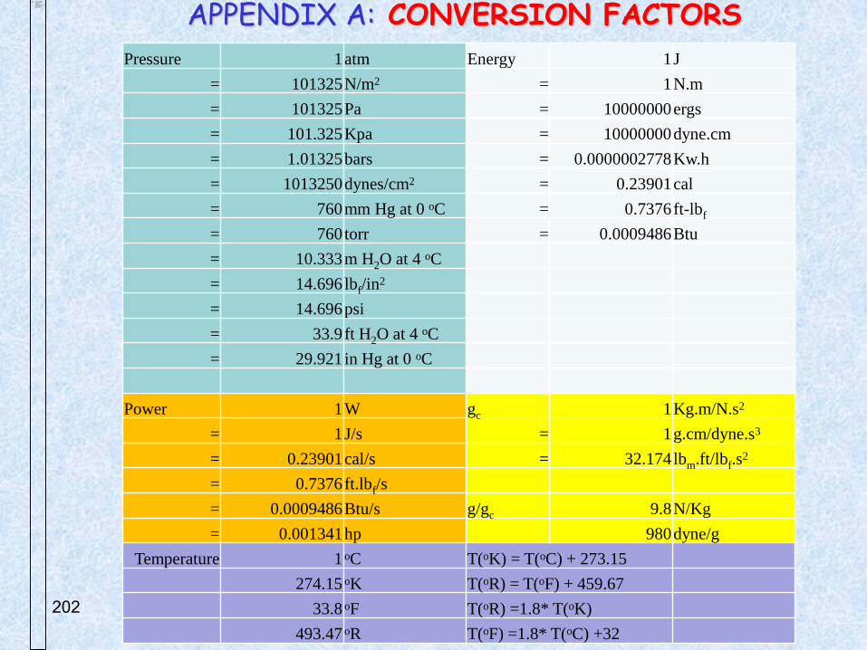
Pressure 1 atm Energy 1 J
= 101325 N/m2 = 1 N.m
= 101325 Pa = 10000000 ergs
= 101.325 Kpa = 10000000 dyne.cm
= 1.01325 bars = 0.0000002778 Kw.h
= 1013250 dynes/cm2 = 0.23901 cal
= 760 mm Hg at 0 oC = 0.7376 ft-lbf
= 760 torr = 0.0009486 Btu
= 10.333 m H2O at 4 oC
= 14.696 lbf/in2
= 14.696 psi
= 33.9 ft H2O at 4 oC
= 29.921 in Hg at 0 oC
Power 1 W gc 1 Kg.m/N.s2
= 1 J/s = 1 g.cm/dyne.s3
= 0.23901 cal/s = 32.174 lbm.ft/lbf.s2
= 0.7376 ft.lbf/s
= 0.0009486 Btu/s g/gc 9.8 N/Kg
= 0.001341 hp 980 dyne/g
Temperature 1 oC T(oK) = T(oC) + 273.15
274.15 oK T(oR) = T(oF) + 459.67
33.8 oF T(oR) =1.8* T(oK)
493.47 oR T(oF) =1.8* T(oC) +32
203
APPENDIX A: CONVERSION FACTORS
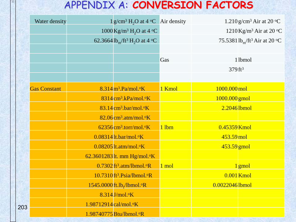
Water density 1 g/cm3 H2O at 4 oC Air density 1.210 g/cm3 Air at 20 oC
1000 Kg/m3 H2O at 4 oC 1210 Kg/m3 Air at 20 oC
62.3664 lbm/ft3 H2O at 4 oC 75.5381 lbm/ft3 Air at 20 oC
Gas 1 lbmol
379 ft3
Gas Constant 8.314 m3.Pa/mol.oK 1 Kmol 1000.000 mol
8314 cm3.kPa/mol.oK 1000.000 gmol
83.14 cm3.bar/mol.oK 2.2046 lbmol
82.06 cm3.atm/mol.oK
62356 cm3.torr/mol.oK 1 lbm 0.45359 Kmol
0.08314 lt.bar/mol.oK 453.59 mol
0.08205 lt.atm/mol.oK 453.59 gmol
62.3601283 lt. mm Hg/mol.oK
0.7302 ft3.atm/lbmol.oR 1 mol 1 gmol
10.7310 ft3.Psia/lbmol.oR 0.001 Kmol
1545.0000 ft.lbf/lbmol.oR 0.0022046 lbmol
8.314 J/mol.oK
1.98712914 cal/mol.oK
1.98740775 Btu/lbmol.oR