Embed Size (px)
DESCRIPTION
transportation civil pe exam problems
Citation preview

www.passpe.com Transportation Module for Civil PE License © Dr. Shahin A.Mansour, PE
Transportaion Engineering Module
for Civil PE License
Separate Breadth (AM) & Depth (PM) Topics Per NCEES
A Concise & Comprehensive Summary of Construction Engineering Equations (Code & Non-Code), Tables, Charts, and Figures is Provided for a Quick Access in the Exam
Dr. Shahin A. Mansour, PE
First Edition
Well Organized, Based on the Latest California Board Test Plan and NCEES Exam Specifications, Detailed Tables of Contents, Computer Generated Index (12 pages), Simplified Concepts, 104 Practice Problems with Detailed Solutions.
The only book that has: • A comprehensive summary of equations, tables, and
charts you need for the exam. All what you need at one location and at your fingertips.
• Separate AM and PM topics. Focus and study only the sections you need.
www.passpe.com Transportation for Civil PE License © Dr. Shahin A.Mansour, PE
ISBN ????????? © 2011 Professional Engineering Services (PES)
All rights reserved. No part of this book may be reproduced by any means, without a written permission from the author.
The author can be reached by email: [email protected]
Current printing of this edition 1
Printed in the United States of America Library of Congress Control Number:
www.passpe.com Transportation Module for Civil PE License © Dr. Shahin A.Mansour, PE
Preface
ur next generation of Civil PE books were carefully developed by Dr. Shahin A. Mansour, Ph.D., P.E., a nationally recognized expert in PE Exam Preparation courses and founder of Professional Engineering Services, Inc., (PES). This generation is quickly becoming the Best in Class solution for engineering professionals working to pass upcoming California Board and NCEES
exams. Each and every book in this comprehensive collection has been prepared with your readiness in mind and will serve as a powerful guide throughout your PE Exam Preparation studies in Civil PE, Seismic, and Surveying concentrations. Dr. Mansour has taught and spoken to thousands of engineers and has been teaching PE, Seismic, Surveying, and EIT/FE classes for the past 22 years enabling his products, classes, and seminars to continuously evolve and adapt to the changing demands of this challenging field. His real-world experience and intercommunication with so many engineers throughout America has greatly improved his ability to craft concise and knowledgeable resources that work for professionals striving to pass their Professional Engineering Licensing Board Exam and other California special exams. One of the primary advantages of PES’ preparation books is their compact and succinct format. The experiences and feedback of engineering students and professionals that have worked with these materials affirms our effective use of good, factual diagrams and illustrations to more fully explain concepts throughout each text. In fact, Dr. Mansour makes great use of this style of teaching through figures, comparative tables, charts, and illustrations to concisely convey important information to engineers preparing for the exam. The primary focus of each book in our collection is targeted on subjects that are directly relevant to the PE exam. This method provides substantial time savings to students that simply don’t have the wherewithal to digest leading competitive volumes, which typically exceed 1,000 pages. Another strong asset of these next generation books is the separation of Breadth (a.m.) and Depth (p.m.) topics. Each Civil PE, Seismic, and Surveying book is organized in accordance with the most current exam specifications and has matured since their inception through the inputs, complaints, wishes, and other feedback given from course participants and colleagues for over 22 years. Recent changes in the format of the Civil PE exam have made it necessary to address the change from essay to multiple choice problems, separation of a.m. and p.m. sections, and the introduction of the construction module. The books’ improved organization is completed with a very detailed Table of Contents, which addresses both the a.m. and p.m. subjects and more, making them a favored resource for preparation as well as exam time. The best part in all this growth and continuous improvement is the ability to apply this knowledge and experience to our supplemental products developed to give you the best head start for passing your Professional Engineering Licensing Board Exam. Every book, DVD, seminar, and accompanying Problems & Solutions workbooks are designed with all relevant codes, topics, board test plans, and NCEES exam specifications. And, these study materials and seminars, also manage to cover these fields of study in the same order as listed in the latest exam specifications for easy reference at-a-glance. Not only are our next generation books written to be current and well-organized to save you time during exam preparation and test taking; they are also affordable and authored by a highly qualified and nationally recognized Civil Engineering Professor. Dr. Shahin A. Mansour, Ph.D., P.E has helped thousands of students to pass their Professional Engineering Licensing Board Exam. His easy, step-by-step approach to solving problems has gained him popularity and a great reputation among students and professionals of all ages. We hope that you’ll find the many resources at Professional Engineering Services, Inc. to be exceptional textbooks, DVDs, and seminars – and as valuable a resource as we believe them to be.
O
www.passpe.com Transportation for Civil PE License © Dr. Shahin A.Mansour, PE
4 NCEES Exam Specifications
Disclaimer
This publication is to help the candidates for the Transportation Module for PE Civil License. This publication expresses the opinion of the author. Every effort and care has been taken to ensure that all data, information, solutions, concepts, and suggestions are as accurate as possible. The author cannot assume or accept the responsibility or liability for errors in the data, information, solutions, concepts, and suggestions and the use of this material in preparation for the exam or using it during the exam. Also, Professional Engineering Services (PES) and the author are in no way responsible for the failure of registrants in the exam, or liable for errors or omission in the solutions, or in the way they are interpreted by the registrants or others.
Errata Notification
PES and the author have made a substantial effort to ensure that the information in this publication is accurate. In the event that corrections or clarifications are needed, those will be posted on the PES web site at http:// www.passpe.com. PES and the author at their discretion, may or may not issue written errata. PES and the author welcome comments or corrections which can be emailed to [email protected]
How to Use This Book
This book was written to help you prepare for the PE-Civil. The following is a suggested strategy preparation for the exam:
1- Have all references organized before you start. Also, familiarize yourself with the comprehensive summary provided in this book.
2- Read the questions and ALL answers carefully and look for KEY WORDS in the question and the 4 possible answers.
3- Solve the easy questions first (ones that need no or minimum calculations) and record your answers on the answer sheet.
4- Work on questions that require lengthy calculations and record your answers on the answer sheet. 5- Questions that seem difficult or not familiar to you and may need considerable time in searching in
your references should be left to the end 6- Never leave an answer blank 7- Remember the D3 rule:
DO NOT EXPECT THE EXAM TO BE EASY DO NOT PANIC DO NOT WASTE TOO MUCH TIME ON A SIGNLE EASY, DIFFICULT, OR
UNFAMILAR PROBLEM
About the Author
Dr. Shahin A. Mansour, PE, has been teaching PE, Seismic, Surveying and EIT courses for the last 22 years. Dr. Mansour taught Civil Engineering Courses for 7 years at New Mexico State University (NMSU), Las Cruces, NM, USA. Also, he has been teaching Civil and Construction Engineering Courses (graduate & undergraduate) at CSU, Fresno, CA, for the last 20 years. Dr. Mansour has helped thousands of students to pass their Professional Engineering Licensing Board Exam. His easy, step-by-step approach to solving problems has gained him popularity and a great reputation among students and professionals of all ages.
www.passpe.com Transportation Module for Civil PE License © Dr. Shahin A.Mansour, PE
General Table of Contents 5
TABLE OF CONTENTS Preface………………………………………………………………………………… Study Tips and Suggested Exam Strategy …………………………………………… NCEES New Format for the PE (Civil) Exam……………………………………….. List of References per NCEES ………………………………………………………. Summary of the Equations …………………………………………………………..
Breadth (A.M.) Topics
1. Horizontal curves …………………………………………………………….. 2. Vertical curves ……………………………………………………………….. 3. Sight distance ………………………………………………………………… 4. Superelevation ……………………………………………………………….. 5. Vertical and/or horizontal clearances ……………………………………….. 6. Acceleration and deceleration ……………………………………………......
Depth (P.M.) Topics
1. Traffic capacity studies …………………………………………………….. 2. Traffic signals ………………………………………………………………. 3. Speed studies ……………………………………………………………….. 4. Intersection analysis ……………………………………………………….. 5. Traffic volume studies……………………………………………………... 6. Sight distance evaluation …………………………………………………... 7. Traffic control devices……………………………………………………… 8. Pedestrian facilities…………………………………………………………. 9. Driver behavior and/or performance ………………………………………. 10. Intersections and/or interchanges ………………………………………….. 11. Optimization and/or cost analysis (e.g., transportation route A or transportation
route B) …………………………………………………………………….. 12. Traffic impact studies ………………………………………………………. 13. Capacity analysis (future conditions)………………………………………. 14. Roadside clearance analysis ……………………………………………… 15. Conflict analysis …………………………………………………………… 16. Work zone safety …………………………………………………………… 17. Accident analysis …………………………………………………………… 18. Hydraulics 1. Culvert design……………………………………………………………
2. Open channel – subcritical and supercritical flow……………………… 19. Hydrology
1. Hydrograph development and synthetic hydrographs……………………
www.passpe.com Transportation for Civil PE License © Dr. Shahin A.Mansour, PE
6 NCEES Exam Specifications
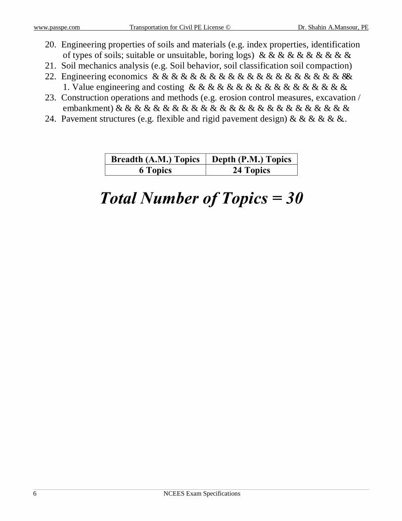
20. Engineering properties of soils and materials (e.g. index properties, identification of types of soils; suitable or unsuitable, boring logs) ………………………….
21. Soil mechanics analysis (e.g. Soil behavior, soil classification soil compaction) 22. Engineering economics …………………………………………………………
1. Value engineering and costing …………………………………………….. 23. Construction operations and methods (e.g. erosion control measures, excavation /
embankment)………………………………………………………………… 24. Pavement structures (e.g. flexible and rigid pavement design)………………..
Breadth (A.M.) Topics Depth (P.M.) Topics 6 Topics 24 Topics
Total Number of Topics = 30
www.passpe.com Transportation Module for Civil PE License © Dr. Shahin A.Mansour, PE
NCEES Exam Specifications 7
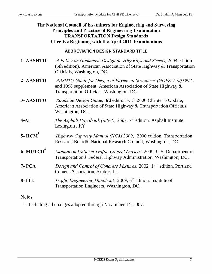
The National Council of Examiners for Engineering and Surveying
Principles and Practice of Engineering Examination TRANSPORTATION Design Standards
Effective Beginning with the April 2011 Examinations
ABBREVIATION DESIGN STANDARD TITLE
1- AASHTO A Policy on Geometric Design of Highways and Streets, 2004 edition (5th edition), American Association of State Highway & Transportation Officials, Washington, DC.
2- AASHTO AASHTO Guide for Design of Pavement Structures (GDPS-4-M)1993,, and 1998 supplement, American Association of State Highway & Transportation Officials, Washington, DC.
3- AASHTO Roadside Design Guide, 3rd edition with 2006 Chapter 6 Update, American Association of State Highway & Transportation Officials, Washington, DC.
4-AI The Asphalt Handbook (MS-4), 2007, 7th edition, Asphalt Institute, Lexington , KY
5- HCM1
Highway Capacity Manual (HCM 2000), 2000 edition, Transportation Research Board—National Research Council, Washington, DC.
6- MUTCD2
Manual on Uniform Traffic Control Devices, 2009, U.S. Department of Transportation—Federal Highway Administration, Washington, DC.
7- PCA Design and Control of Concrete Mixtures, 2002, 14th edition, Portland Cement Association, Skokie, IL.
8- ITE Traffic Engineering Handbook, 2009, 6th edition, Institute of Transportation Engineers, Washington, DC.
Notes 1. Including all changes adopted through November 14, 2007.
www.passpe.com Transportation for Civil PE License © Dr. Shahin A.Mansour, PE
8 NCEES Exam Specifications
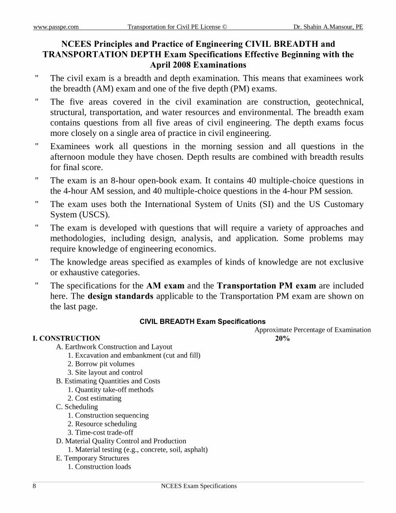
NCEES Principles and Practice of Engineering CIVIL BREADTH and TRANSPORTATION DEPTH Exam Specifications Effective Beginning with the
April 2008 Examinations
• The civil exam is a breadth and depth examination. This means that examinees work the breadth (AM) exam and one of the five depth (PM) exams.
• The five areas covered in the civil examination are construction, geotechnical, structural, transportation, and water resources and environmental. The breadth exam contains questions from all five areas of civil engineering. The depth exams focus more closely on a single area of practice in civil engineering.
• Examinees work all questions in the morning session and all questions in the afternoon module they have chosen. Depth results are combined with breadth results for final score.
• The exam is an 8-hour open-book exam. It contains 40 multiple-choice questions in the 4-hour AM session, and 40 multiple-choice questions in the 4-hour PM session.
• The exam uses both the International System of Units (SI) and the US Customary System (USCS).
• The exam is developed with questions that will require a variety of approaches and methodologies, including design, analysis, and application. Some problems may require knowledge of engineering economics.
• The knowledge areas specified as examples of kinds of knowledge are not exclusive or exhaustive categories.
• The specifications for the AM exam and the Transportation PM exam are included here. The design standards applicable to the Transportation PM exam are shown on the last page.
CIVIL BREADTH Exam Specifications
Approximate Percentage of Examination I. CONSTRUCTION 20%
A. Earthwork Construction and Layout 1. Excavation and embankment (cut and fill) 2. Borrow pit volumes 3. Site layout and control
B. Estimating Quantities and Costs 1. Quantity take-off methods 2. Cost estimating
C. Scheduling 1. Construction sequencing 2. Resource scheduling 3. Time-cost trade-off
D. Material Quality Control and Production 1. Material testing (e.g., concrete, soil, asphalt)
E. Temporary Structures 1. Construction loads
www.passpe.com Transportation Module for Civil PE License © Dr. Shahin A.Mansour, PE
NCEES Exam Specifications 9
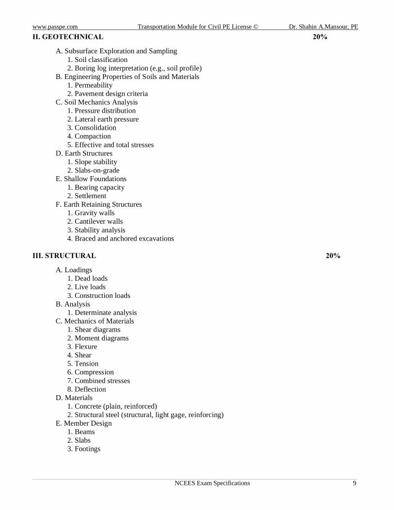
II. GEOTECHNICAL 20% A. Subsurface Exploration and Sampling
1. Soil classification 2. Boring log interpretation (e.g., soil profile)
B. Engineering Properties of Soils and Materials 1. Permeability 2. Pavement design criteria
C. Soil Mechanics Analysis 1. Pressure distribution 2. Lateral earth pressure 3. Consolidation 4. Compaction 5. Effective and total stresses
D. Earth Structures 1. Slope stability 2. Slabs-on-grade
E. Shallow Foundations 1. Bearing capacity 2. Settlement
F. Earth Retaining Structures 1. Gravity walls 2. Cantilever walls 3. Stability analysis 4. Braced and anchored excavations
III. STRUCTURAL 20%
A. Loadings
1. Dead loads 2. Live loads 3. Construction loads
B. Analysis 1. Determinate analysis
C. Mechanics of Materials 1. Shear diagrams 2. Moment diagrams 3. Flexure 4. Shear 5. Tension 6. Compression 7. Combined stresses 8. Deflection
D. Materials 1. Concrete (plain, reinforced) 2. Structural steel (structural, light gage, reinforcing)
E. Member Design 1. Beams 2. Slabs 3. Footings
www.passpe.com Transportation for Civil PE License © Dr. Shahin A.Mansour, PE
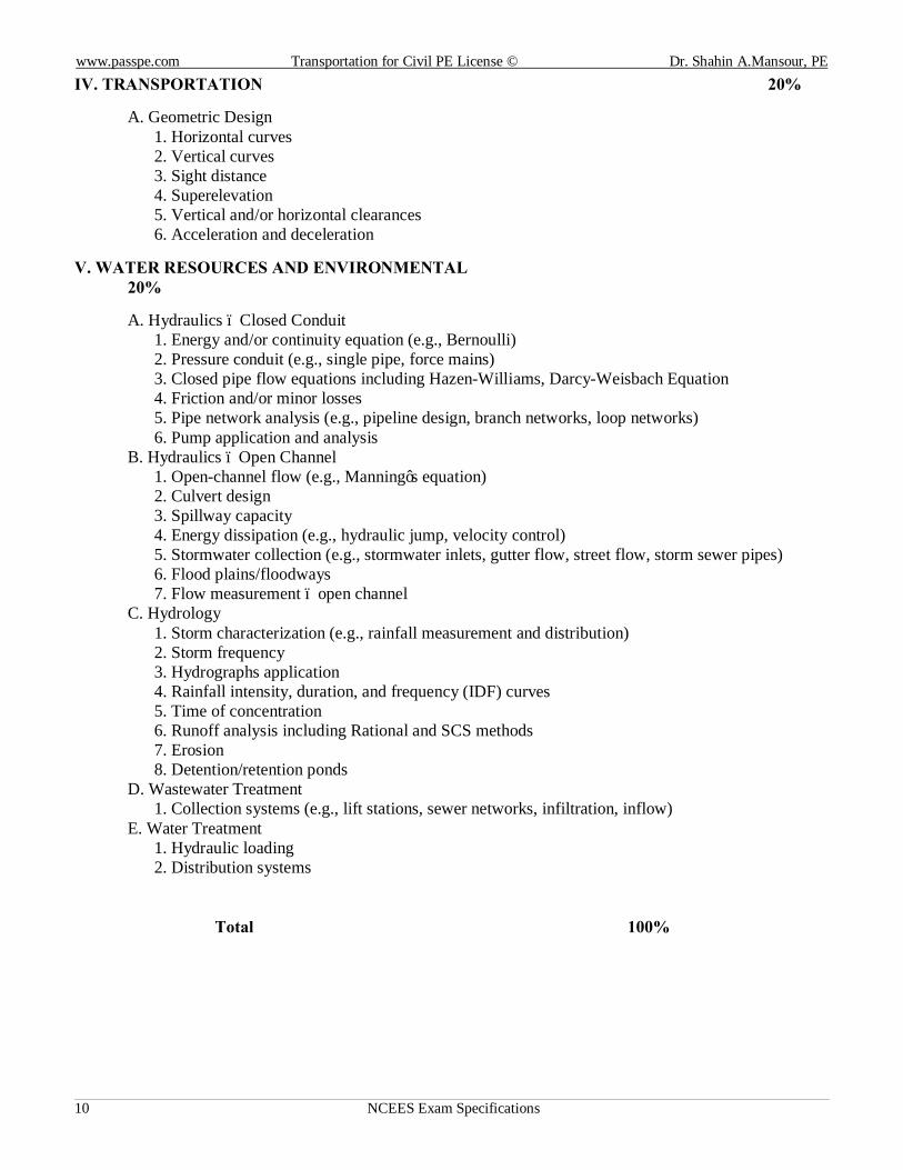
10 NCEES Exam Specifications
IV. TRANSPORTATION 20% A. Geometric Design
1. Horizontal curves 2. Vertical curves 3. Sight distance 4. Superelevation 5. Vertical and/or horizontal clearances 6. Acceleration and deceleration
V. WATER RESOURCES AND ENVIRONMENTAL 20% A. Hydraulics – Closed Conduit
1. Energy and/or continuity equation (e.g., Bernoulli) 2. Pressure conduit (e.g., single pipe, force mains) 3. Closed pipe flow equations including Hazen-Williams, Darcy-Weisbach Equation 4. Friction and/or minor losses 5. Pipe network analysis (e.g., pipeline design, branch networks, loop networks) 6. Pump application and analysis
B. Hydraulics – Open Channel 1. Open-channel flow (e.g., Manning’s equation) 2. Culvert design 3. Spillway capacity 4. Energy dissipation (e.g., hydraulic jump, velocity control) 5. Stormwater collection (e.g., stormwater inlets, gutter flow, street flow, storm sewer pipes) 6. Flood plains/floodways 7. Flow measurement – open channel
C. Hydrology 1. Storm characterization (e.g., rainfall measurement and distribution) 2. Storm frequency 3. Hydrographs application 4. Rainfall intensity, duration, and frequency (IDF) curves 5. Time of concentration 6. Runoff analysis including Rational and SCS methods 7. Erosion 8. Detention/retention ponds
D. Wastewater Treatment 1. Collection systems (e.g., lift stations, sewer networks, infiltration, inflow)
E. Water Treatment 1. Hydraulic loading 2. Distribution systems
Total 100%
www.passpe.com Transportation Module for Civil PE License © Dr. Shahin A.Mansour, PE
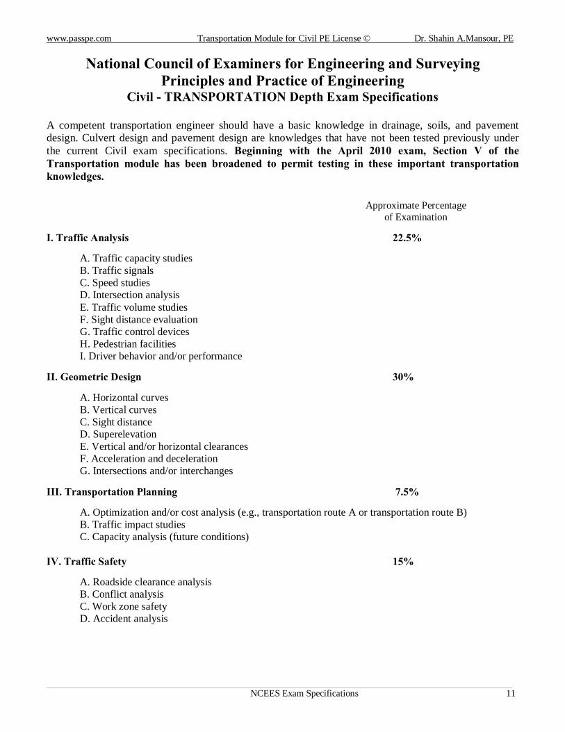
NCEES Exam Specifications 11
National Council of Examiners for Engineering and Surveying Principles and Practice of Engineering
Civil - TRANSPORTATION Depth Exam Specifications
A competent transportation engineer should have a basic knowledge in drainage, soils, and pavement design. Culvert design and pavement design are knowledges that have not been tested previously under the current Civil exam specifications. Beginning with the April 2010 exam, Section V of the Transportation module has been broadened to permit testing in these important transportation knowledges.
Approximate Percentage of Examination
I. Traffic Analysis 22.5%
A. Traffic capacity studies B. Traffic signals C. Speed studies D. Intersection analysis E. Traffic volume studies F. Sight distance evaluation G. Traffic control devices H. Pedestrian facilities I. Driver behavior and/or performance
II. Geometric Design 30%
A. Horizontal curves B. Vertical curves C. Sight distance D. Superelevation E. Vertical and/or horizontal clearances F. Acceleration and deceleration G. Intersections and/or interchanges
III. Transportation Planning 7.5%
A. Optimization and/or cost analysis (e.g., transportation route A or transportation route B) B. Traffic impact studies C. Capacity analysis (future conditions)
IV. Traffic Safety 15%
A. Roadside clearance analysis B. Conflict analysis C. Work zone safety D. Accident analysis
www.passpe.com Transportation for Civil PE License © Dr. Shahin A.Mansour, PE
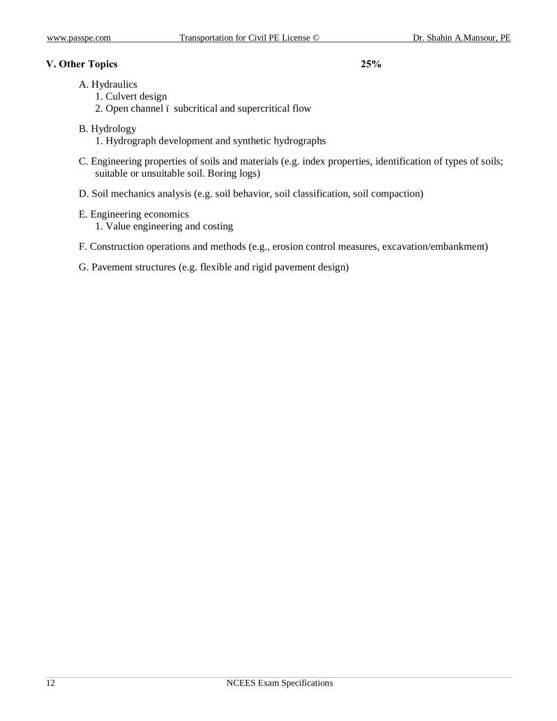
12 NCEES Exam Specifications
V. Other Topics 25%
A. Hydraulics
1. Culvert design 2. Open channel – subcritical and supercritical flow
B. Hydrology 1. Hydrograph development and synthetic hydrographs
C. Engineering properties of soils and materials (e.g. index properties, identification of types of soils; suitable or unsuitable soil. Boring logs)
D. Soil mechanics analysis (e.g. soil behavior, soil classification, soil compaction)
E. Engineering economics 1. Value engineering and costing
F. Construction operations and methods (e.g., erosion control measures, excavation/embankment) G. Pavement structures (e.g. flexible and rigid pavement design)
www.passpe.com Transportation for Civil PE License © Dr. Shahin A.Mansour, PE
Summary of Transportation Engineering Equations and Topics 13
A CONCISE & COMPREHENSIVE SUMMARY
Of TRANSPORTATION
MODULE
EQUATIONS & TOPICS Codes Equations, Non-Code Equations, Tables,
Flow Charts, and Figures Per NCEES List of Topics and Exam
Specifications
www.passpe.com Transportation for Civil PE License © Dr. Shahin A.Mansour, PE
Part I- Civil Breadth (Transportation A.M.) - Chapter A: Geometric Design 14
I. Traffic Analysis 22.5% (9 questions)
www.passpe.com Transportation for Civil PE License © Dr. Shahin A.Mansour, PE
Summary of Transportation Engineering Equations and Topics 15
II.Geometric Design 30% (12 questions)
www.passpe.com Transportation for Civil PE License © Dr. Shahin A.Mansour, PE
Part I- Civil Breadth (Transportation A.M.) - Chapter A: Geometric Design 16
III. Transportation Planning 7.5% (3 questions)
www.passpe.com Transportation for Civil PE License © Dr. Shahin A.Mansour, PE
Summary of Transportation Engineering Equations and Topics 17
IV. Traffic Safety 15% (6 questions)

www.passpe.com Transportation for Civil PE License © Dr. Shahin A.Mansour, PE
Part I- Civil Breadth (Transportation A.M.) - Chapter A: Geometric Design 18
V. Other Topics 25% (10 questions)
www.passpe.com Transportation for Civil PE License © Dr. Shahin A.Mansour, PE
Summary of Transportation Engineering Equations and Topics 19
This page is left intentionally blank for additional summary of equations
www.passpe.com Transportation for Civil PE License © Dr. Shahin A.Mansour, PE
Part I- Civil Breadth (Transportation A.M.) - Chapter A: Geometric Design 20
This page is left intentionally blank for additional summary of equations
www.passpe.com Transportation for Civil PE License © Dr. Shahin A.Mansour, PE
Summary of Transportation Engineering Equations and Topics 21
www.passpe.com Transportation for Civil PE License © Dr. Shahin A.Mansour, PE
Part I- Civil Breadth (Transportation A.M.) - Chapter A: Geometric Design 22
PART 1
Civil BREADTH (A.M.) Exam Specifications
TRANSPORTATION
www.passpe.com Transportation for Civil Engineering (PE) License © Dr. Shahin A. Mansour, PE
Part I- Civil Breadth (Transportation A.M.) - Chapter A: Geometric Design 23
Transportation Breadth (A.M.) Topics
Chapter A: Geometric Design
1. Horizontal curves………………………… ………………………………………24 2. Vertical curves….. ………………………………………………………………..46 3. Sight distance………..…………………………………………………………….57 4. Superelevation…………………………………………………………...………..84 5. Vertical and/or horizontal clearances…………………………….…………….....92 6. Acceleration and deceleration ……………………………………………………99
www.passpe.com Transportation for Civil PE License © Dr. Shahin A.Mansour, PE
Part I- Civil Breadth (Transportation A.M.) - Chapter A: Geometric Design 24
Chapter A: Geometric Design
A.1 HORIZONTAL CURVES
A.1.1 Introduction:
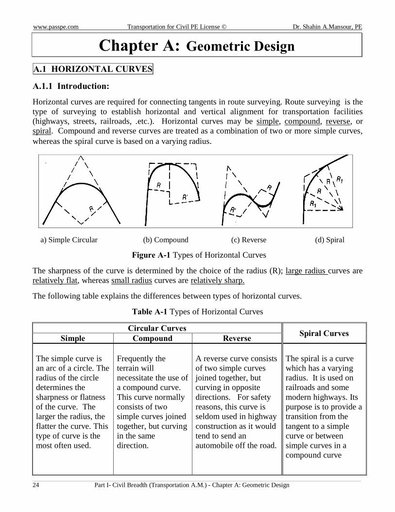
Horizontal curves are required for connecting tangents in route surveying. Route surveying is the type of surveying to establish horizontal and vertical alignment for transportation facilities (highways, streets, railroads, .etc.). Horizontal curves may be simple, compound, reverse, or spiral. Compound and reverse curves are treated as a combination of two or more simple curves, whereas the spiral curve is based on a varying radius.
a) Simple Circular (b) Compound (c) Reverse (d) Spiral
Figure A-1 Types of Horizontal Curves
The sharpness of the curve is determined by the choice of the radius (R); large radius curves are relatively flat, whereas small radius curves are relatively sharp.
The following table explains the differences between types of horizontal curves.
Table A-1 Types of Horizontal Curves
Circular Curves Spiral Curves Simple Compound Reverse The simple curve is an arc of a circle. The radius of the circle determines the sharpness or flatness of the curve. The larger the radius, the flatter the curve. This type of curve is the most often used.
Frequently the terrain will necessitate the use of a compound curve. This curve normally consists of two simple curves joined together, but curving in the same direction.
A reverse curve consists of two simple curves joined together, but curving in opposite directions. For safety reasons, this curve is seldom used in highway construction as it would tend to send an automobile off the road.
The spiral is a curve which has a varying radius. It is used on railroads and some modern highways. Its purpose is to provide a transition from the tangent to a simple curve or between simple curves in a compound curve
www.passpe.com Transportation for Civil Engineering (PE) License © Dr. Shahin A. Mansour, PE
Part I- Civil Breadth (Transportation A.M.) - Chapter A: Geometric Design 25
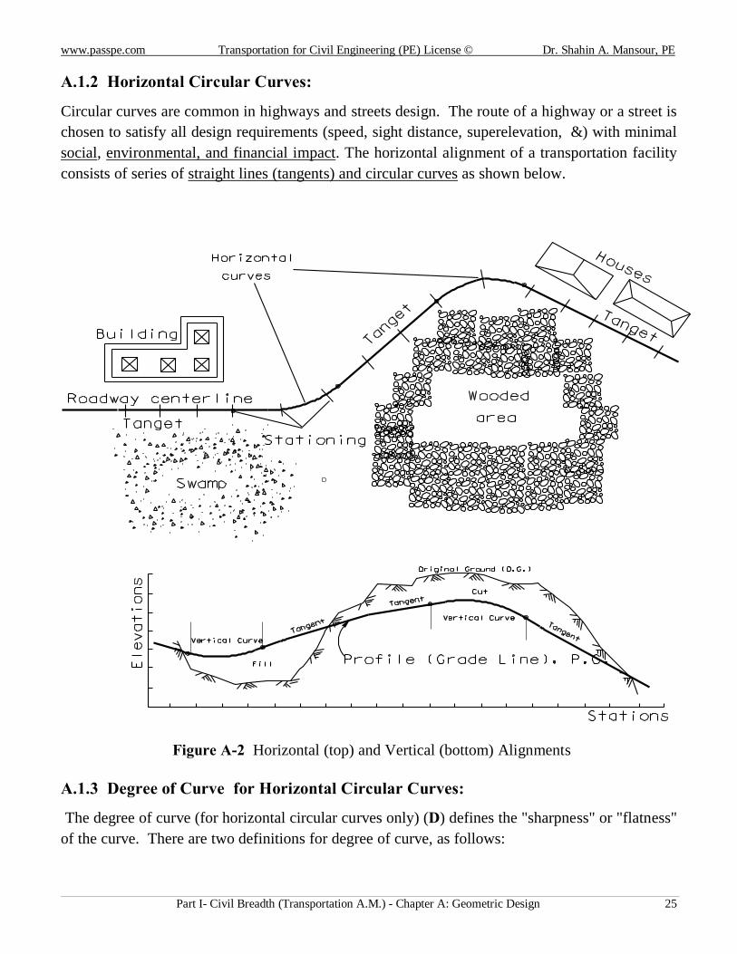
A.1.2 Horizontal Circular Curves:
Circular curves are common in highways and streets design. The route of a highway or a street is chosen to satisfy all design requirements (speed, sight distance, superelevation, …) with minimal social, environmental, and financial impact. The horizontal alignment of a transportation facility consists of series of straight lines (tangents) and circular curves as shown below.
Figure A-2 Horizontal (top) and Vertical (bottom) Alignments A.1.3 Degree of Curve for Horizontal Circular Curves:
The degree of curve (for horizontal circular curves only) (D) defines the "sharpness" or "flatness" of the curve. There are two definitions for degree of curve, as follows:
www.passpe.com Transportation for Civil PE License © Dr. Shahin A.Mansour, PE
Part I- Civil Breadth (Transportation A.M.) - Chapter A: Geometric Design 26
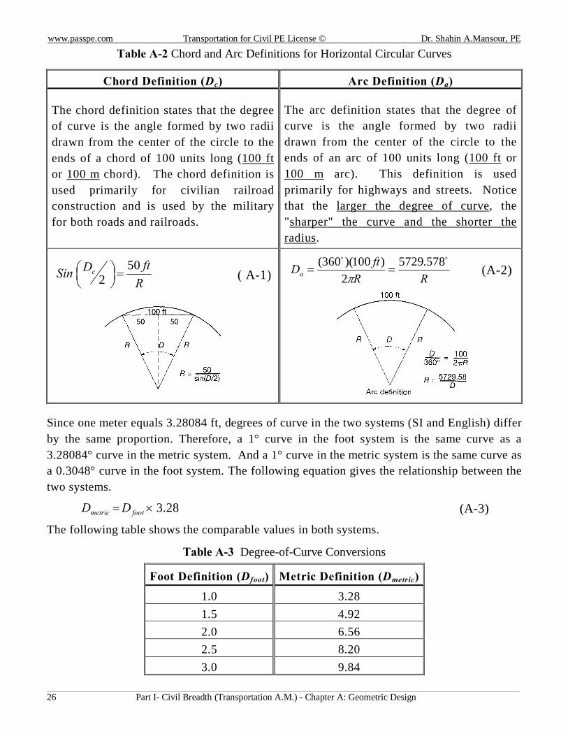
Table A-2 Chord and Arc Definitions for Horizontal Circular Curves
Chord Definition (Dc) Arc Definition (Da) The chord definition states that the degree of curve is the angle formed by two radii drawn from the center of the circle to the ends of a chord of 100 units long (100 ft or 100 m chord). The chord definition is used primarily for civilian railroad construction and is used by the military for both roads and railroads.
The arc definition states that the degree of curve is the angle formed by two radii drawn from the center of the circle to the ends of an arc of 100 units long (100 ft or 100 m arc). This definition is used primarily for highways and streets. Notice that the larger the degree of curve, the "sharper" the curve and the shorter the radius.
RftDSin c 50
2 =
( A-1)
RRftDa
oo 578.57292
)100)(360(==
π (A-2)
Since one meter equals 3.28084 ft, degrees of curve in the two systems (SI and English) differ by the same proportion. Therefore, a 1° curve in the foot system is the same curve as a 3.28084° curve in the metric system. And a 1° curve in the metric system is the same curve as a 0.3048° curve in the foot system. The following equation gives the relationship between the two systems.
28.3×= footmetric DD (A-3) The following table shows the comparable values in both systems.
Table A-3 Degree-of-Curve Conversions
Foot Definition (Dfoot) Metric Definition (Dmetric) 1.0 3.28 1.5 4.92 2.0 6.56 2.5 8.20 3.0 9.84
www.passpe.com Transportation for Civil Engineering (PE) License © Dr. Shahin A. Mansour, PE
Part I- Civil Breadth (Transportation A.M.) - Chapter A: Geometric Design 27
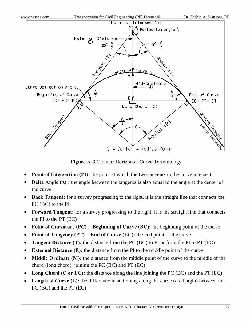
Figure A-3 Circular Horizontal Curve Terminology
• Point of Intersection (PI): the point at which the two tangents to the curve intersect • Delta Angle (Δ) : the angle between the tangents is also equal to the angle at the center of
the curve • Back Tangent: for a survey progressing to the right, it is the straight line that connects the
PC (BC) to the PI • Forward Tangent: for a survey progressing to the right, it is the straight line that connects
the PI to the PT (EC) • Point of Curvature (PC) = Beginning of Curve (BC): the beginning point of the curve • Point of Tangency (PT) = End of Curve (EC): the end point of the curve • Tangent Distance (T): the distance from the PC (BC) to PI or from the PI to PT (EC) • External Distance (E): the distance from the PI to the middle point of the curve • Middle Ordinate (M): the distance from the middle point of the curve to the middle of the
chord (long chord) joining the PC (BC) and PT (EC) • Long Chord (C or LC): the distance along the line joining the PC (BC) and the PT (EC) • Length of Curve (L): the difference in stationing along the curve (arc length) between the
PC (BC) and the PT (EC)
www.passpe.com Transportation for Civil PE License © Dr. Shahin A.Mansour, PE
Part I- Civil Breadth (Transportation A.M.) - Chapter A: Geometric Design 28
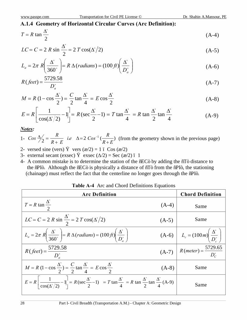
A.1.4 Geometry of Horizontal Circular Curves (Arc Definition):
2tan
o∆= RT (A-4)
)2cos(22
sin2 oo
∆=∆
== TRCLC (A-5)
∆=∆=
∆=
o
o
o
o
aa D
ftradiansRRL )100()(360
2π (A-6)
oaD
feetR 58.5729)( = (A-7)
2cos
4tan
2)
2cos1(
ooo ∆=
∆=
∆−= ECRM (A-8)
4tan
2tan
4tan)1
2(sec1
)2cos(1 oooo
o
∆∆=∆=−∆=
−
∆= RTRRE (A-9)
Notes:
1- )(2.21
ERRCosei
ERRCos
+=∆
+=∆ − (from the geometry shown in the previous page)
2- versed sine (vers) → vers (∆/2) = 1 − Cos (∆/2) 3- external secant (exsec) → exsec (∆/2) = Sec (∆/2) − 1 4- A common mistake is to determine the station of the “EC” by adding the “T” distance to the “PI”. Although the “EC” is physically a distance of “T” from the “PI”, the stationing (chainage) must reflect the fact that the centerline no longer goes through the “PI”.
Table A-4 Arc and Chord Definitions Equations
Arc Definition Chord Definition
2tan
o∆= RT (A-4)
Same
)2cos(22
sin2 oo
∆=∆
== TRCLC (A-5) Same
∆=∆=
∆=
o
o
o
o
aa D
ftradiansRRL )100()(360
2π (A-6)
∆=
o
o
cc D
mL )100(
oaD
feetR 58.5729)( = (A-7) oCD
meterR 65.5729)( =
2cos
4tan
2)
2cos1(
ooo ∆=
∆=
∆−= ECRM (A-8) Same
4tan
2tan
4tan)1
2(sec1
)2cos(1 oooo
o
∆∆=
∆=−
∆=
−
∆= RTRRE (A-9) Same
www.passpe.com Transportation for Civil Engineering (PE) License © Dr. Shahin A. Mansour, PE
Part I- Civil Breadth (Transportation A.M.) - Chapter A: Geometric Design 29
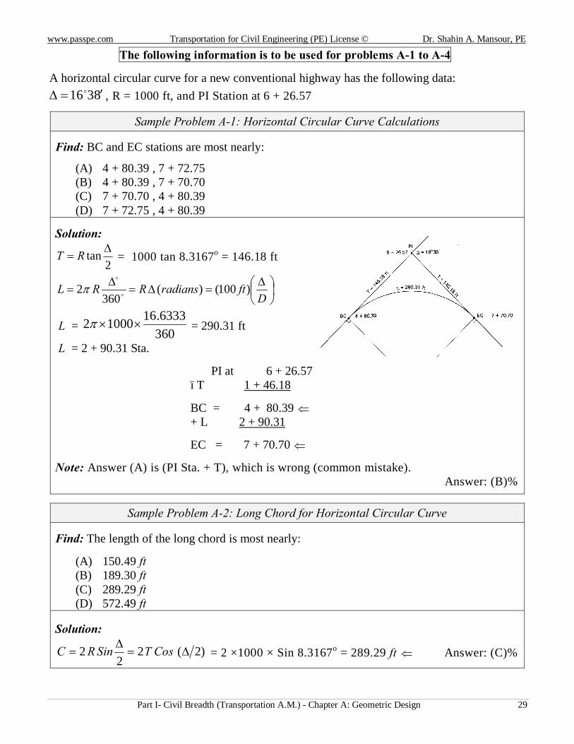
The following information is to be used for problems A-1 to A-4
A horizontal circular curve for a new conventional highway has the following data: 8316 ′=∆ o , R = 1000 ft, and PI Station at 6 + 26.57
Sample Problem A-1: Horizontal Circular Curve Calculations
Find: BC and EC stations are most nearly:
(A) 4 + 80.39 , 7 + 72.75 (B) 4 + 80.39 , 7 + 70.70 (C) 7 + 70.70 , 4 + 80.39 (D) 7 + 72.75 , 4 + 80.39
Solution:
2tan ∆
= RT = 1000 tan 8.3167o = 146.18 ft
∆
=∆=∆
=D
ftradiansRRL )100()(360
2o
o
π
L = 3606333.1610002 ××π = 290.31 ft
L = 2 + 90.31 Sta.
PI at 6 + 26.57 –T 1 + 46.18
BC = 4 + 80.39 ⇐ + L 2 + 90.31
EC = 7 + 70.70 ⇐
Note: Answer (A) is (PI Sta. + T), which is wrong (common mistake). Answer: (B)◄
Sample Problem A-2: Long Chord for Horizontal Circular Curve
Find: The length of the long chord is most nearly:
(A) 150.49 ft (B) 189.30 ft (C) 289.29 ft (D) 572.49 ft
Solution:
)2(22
2 ∆=∆
= CosTSinRC = 2 ×1000 × Sin 8.3167o = 289.29 ft ⇐ Answer: (C)◄

www.passpe.com Transportation for Civil PE License © Dr. Shahin A.Mansour, PE
Part I- Civil Breadth (Transportation A.M.) - Chapter A: Geometric Design 30
Sample Problem A-3: External Distance for a Horizontal Circular Curve
Find: The external distance (E) for the given curve is most nearly:
(A) 10.23 ft (B) 10.43 ft (C) 10.52 ft (D) 10.63 ft
Solution:
ftCosCos
RE 63.10)1)263.16(
1(1000)1)2(
1( =−=−∆
= ⇐
Answer: (D)◄
Sample Problem A-4: Middle Ordinate for a Horizontal Circular Curve
Find: The middle ordinate for the horizontal circular curve is most nearly: (A) 10.23 ft (B) 10.43 ft (C) 10.52 ft (D) 10.63 ft
Solution:
Refer to Figure A-3 for the definition of “M”
?242
)2
1()( iprelationshwhichCosETanCCosRMBtoAOrdinateMiddle ⇐∆
=∆
=∆
−==
)2
1( ∆−= CosRM = 1000 (1 – Cos 8.3167o) = 10.52 ft ⇐
Answer: (C)◄
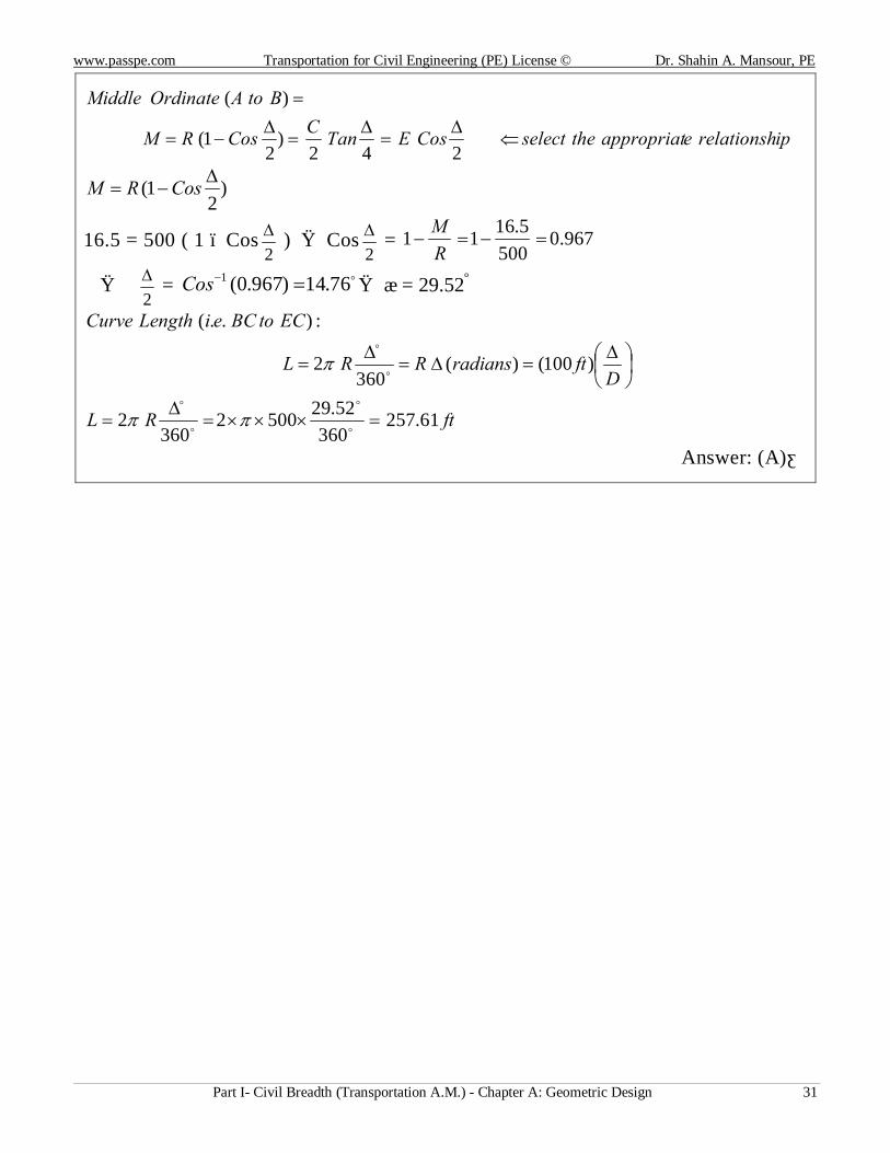
Sample Problem A-5: Length a Horizontal Circular Curve
Given: A horizontal circular curve has a radius of 500 ft, and mid-ordinate of 16.5 ft. Find: The length of the horizontal circular curve is most nearly:
(A) 257.61 ft (B) 265.54 ft (C) 315.45 ft (D) 400.00 ft
Solution:
(Continued on next page)
www.passpe.com Transportation for Civil Engineering (PE) License © Dr. Shahin A. Mansour, PE
Part I- Civil Breadth (Transportation A.M.) - Chapter A: Geometric Design 31
iprelationsheappropriattheselectCosETanCCosRM
BtoAOrdinateMiddle
⇐∆
=∆
=∆
−=
=
242)
21(
)(
)2
1( ∆−= CosRM
16.5 = 500 ( 1 – Cos2∆ ) → Cos
2∆ = 967.0
5005.1611 =−=−
RM
→ 2∆ = o76.14)967.0(1 =−Cos → ∆ = 29.52º
∆
=∆=∆
=D
ftradiansRRL
ECtoBCeiLengthCurve
)100()(360
2
:)..(
o
o
π
ftRL 61.257360
52.295002360
2 =×××=∆
=o
o
o
o
ππ
Answer: (A)◄
www.passpe.com Transportation for Civil PE License © Dr. Shahin A.Mansour, PE
Part I- Civil Breadth (Transportation A.M.) - Chapter A: Geometric Design 32
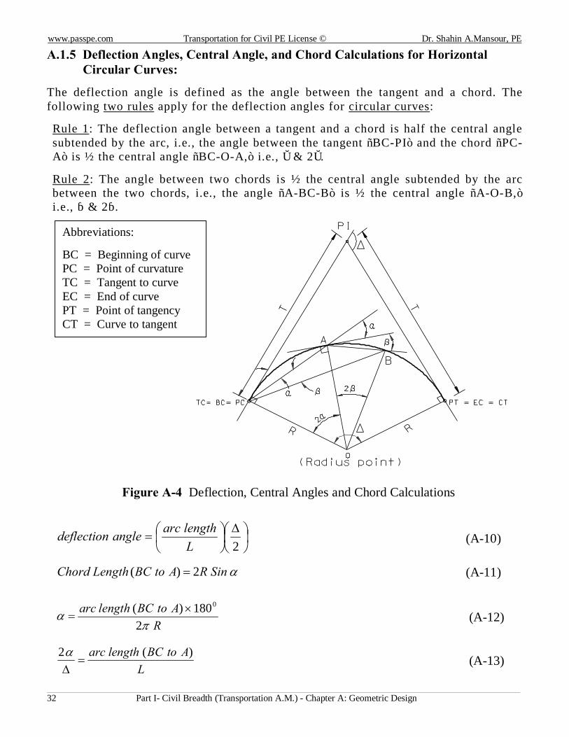
A.1.5 Deflection Angles, Central Angle, and Chord Calculations for Horizontal Circular Curves:
The deflection angle is defined as the angle between the tangent and a chord. The following two rules apply for the deflection angles for circular curves:
Rule 1: The deflection angle between a tangent and a chord is half the central angle subtended by the arc, i.e., the angle between the tangent “BC-PI” and the chord “PC-A” is ½ the central angle “BC-O-A,” i.e., α & 2α.
Rule 2: The angle between two chords is ½ the central angle subtended by the arc between the two chords, i.e., the angle “A-BC-B” is ½ the central angle “A-O-B,” i.e., β & 2β.
Figure A-4 Deflection, Central Angles and Chord Calculations
∆
=
2Llengtharcangledeflection (A-10)
αSinRAtoBCLengthChord 2)( = (A-11)
RAtoBClengtharc
πα
2180)( 0×= (A-12)
LAtoBClengtharc )(2
=∆α
(A-13)
Abbreviations:
BC = Beginning of curve PC = Point of curvature TC = Tangent to curve EC = End of curve PT = Point of tangency CT = Curve to tangent
www.passpe.com Transportation for Civil Engineering (PE) License © Dr. Shahin A. Mansour, PE
Part I- Civil Breadth (Transportation A.M.) - Chapter A: Geometric Design 33
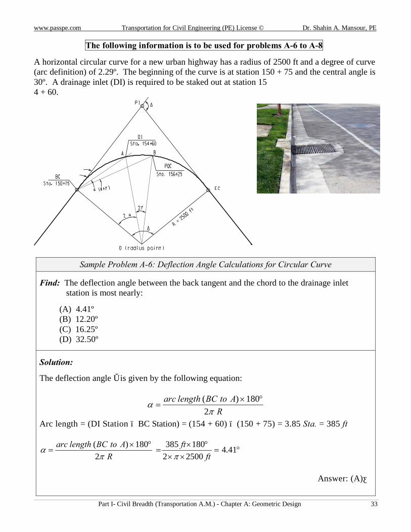
The following information is to be used for problems A-6 to A-8
A horizontal circular curve for a new urban highway has a radius of 2500 ft and a degree of curve (arc definition) of 2.29º. The beginning of the curve is at station 150 + 75 and the central angle is 30º. A drainage inlet (DI) is required to be staked out at station 15 4 + 60.
Sample Problem A-6: Deflection Angle Calculations for Circular Curve
Find: The deflection angle between the back tangent and the chord to the drainage inlet station is most nearly:
(A) 4.41º (B) 12.20º (C) 16.25º (D) 32.50º
Solution:
The deflection angle α is given by the following equation:
RAtoBClengtharc
πα
2180)( °×
=
Arc length = (DI Station − BC Station) = (154 + 60) − (150 + 75) = 3.85 Sta. = 385 ft
°=××
°×=
°×= 41.4
25002180385
2180)(
ftft
RAtoBClengtharc
ππα
Answer: (A)◄
www.passpe.com Transportation for Civil PE License © Dr. Shahin A.Mansour, PE
Part I- Civil Breadth (Transportation A.M.) - Chapter A: Geometric Design 34
Sample Problem A-7: Chord Calculations for Circular Curve
Find: The length of the chord connecting the BC and the drainage inlet is most nearly:
(A) 175.30 ft (B) 254.52 ft (C) 325.15 ft (D) 384.47 ft
Solution:
ftSinftSinRAtoBCeiDItoBCLengthChord 47.38441.4250022)..,( =°××== α
Answer: (D)◄
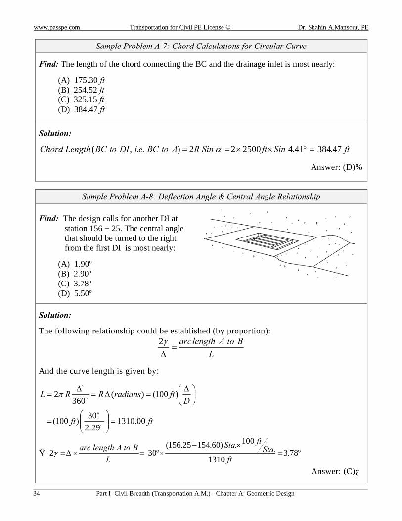
Sample Problem A-8: Deflection Angle & Central Angle Relationship Find: The design calls for another DI at
station 156 + 25. The central angle that should be turned to the right from the first DI is most nearly:
(A) 1.90º (B) 2.90º (C) 3.78º (D) 5.50º
Solution:
The following relationship could be established (by proportion):
LBtoAlengtharc
=∆γ2
And the curve length is given by:
ftft
DftradiansRRL
00.131029.2
30)100(
)100()(360
2
=
=
∆
=∆=∆
=
o
o
o
o
π
→ °=×−
×°=×∆= 78.31310
.100.)60.15425.156(
302ft
StaftSta
LBtoAlengtharcγ
Answer: (C)◄
www.passpe.com Transportation for Civil Engineering (PE) License © Dr. Shahin A. Mansour, PE
Part I- Civil Breadth (Transportation A.M.) - Chapter A: Geometric Design 35
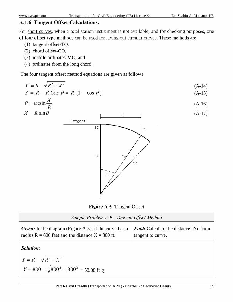
A.1.6 Tangent Offset Calculations:
For short curves, when a total station instrument is not available, and for checking purposes, one of four offset-type methods can be used for laying out circular curves. These methods are:
(1) tangent offset-TO, (2) chord offset-CO, (3) middle ordinates-MO, and (4) ordinates from the long chord.
The four tangent offset method equations are given as follows:
22 XRRY −−= (A-14) )cos1( θθ −=−= RCosRRY (A-15)
RXarcsin=θ (A-16)
θsinRX = (A-17)
Figure A-5 Tangent Offset
Sample Problem A-9: Tangent Offset Method
Given: In the diagram (Figure A-5), if the curve has a radius R = 800 feet and the distance X = 300 ft.
Find: Calculate the distance “Y” from tangent to curve.
Solution:
22 XRRY −−=
=−−= 22 300800800Y 58.38 ft ◄
www.passpe.com Transportation for Civil PE License © Dr. Shahin A.Mansour, PE
Part I- Civil Breadth (Transportation A.M.) - Chapter A: Geometric Design 36
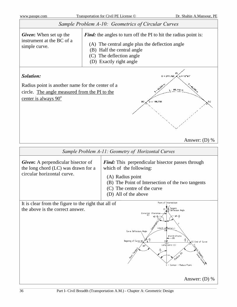
Sample Problem A-10: Geometrics of Circular Curves
Given: When set up the instrument at the BC of a simple curve.
Find: the angles to turn off the PI to hit the radius point is:
(A) The central angle plus the deflection angle (B) Half the central angle
(C) The deflection angle (D) Exactly right angle
Solution:
Radius point is another name for the center of a circle. The angle measured from the PI to the center is always 90o
Answer: (D) ◄
Sample Problem A-11: Geometry of Horizontal Curves
Given: A perpendicular bisector of the long chord (LC) was drawn for a circular horizontal curve.
Find: This perpendicular bisector passes through which of the following:
(A) Radius point (B) The Point of Intersection of the two tangents (C) The centre of the curve (D) All of the above
It is clear from the figure to the right that all of the above is the correct answer.
Answer: (D) ◄
www.passpe.com Transportation for Civil Engineering (PE) License © Dr. Shahin A. Mansour, PE
Part I- Civil Breadth (Transportation A.M.) - Chapter A: Geometric Design 37
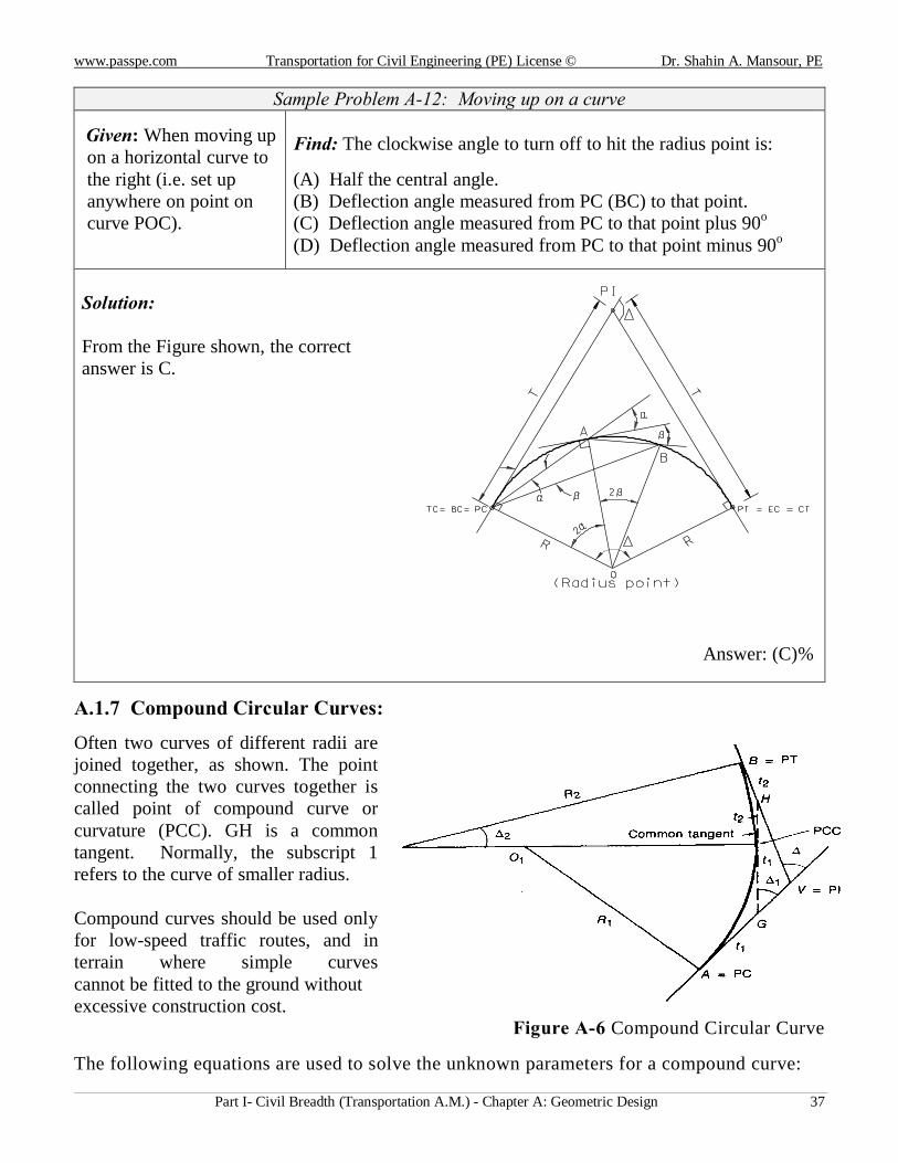
Sample Problem A-12: Moving up on a curve
Given: When moving up on a horizontal curve to the right (i.e. set up anywhere on point on curve POC).
Find: The clockwise angle to turn off to hit the radius point is:
(A) Half the central angle. (B) Deflection angle measured from PC (BC) to that point. (C) Deflection angle measured from PC to that point plus 90o
(D) Deflection angle measured from PC to that point minus 90o
Solution: From the Figure shown, the correct answer is C.
Answer: (C)◄
A.1.7 Compound Circular Curves:
Often two curves of different radii are joined together, as shown. The point connecting the two curves together is called point of compound curve or curvature (PCC). GH is a common tangent. Normally, the subscript 1 refers to the curve of smaller radius. Compound curves should be used only for low-speed traffic routes, and in terrain where simple curves cannot be fitted to the ground without excessive construction cost.
Figure A-6 Compound Circular Curve
The following equations are used to solve the unknown parameters for a compound curve:
www.passpe.com Transportation for Civil PE License © Dr. Shahin A.Mansour, PE
Part I- Civil Breadth (Transportation A.M.) - Chapter A: Geometric Design 38
1221 ∆−∆=∆∆−∆=∆ OR (A-18)
2tan&
2tan 2
221
11∆
=∆
= RtRt (A-19)
21 ttGH += (A-20)
∆
∆=sin
)(sin 2GHVG (A-21)
∆
∆=sin
)(sin 1GHVH (A-22)
11 tVGVAT +== (A-23) 22 tVHVBT +== (A-24)
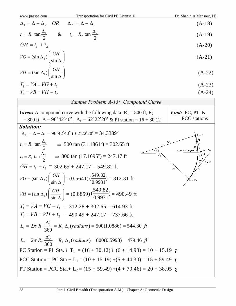
Sample Problem A-13: Compound Curve
Given: A compound curve with the following data: R1 = 500 ft, R2 = 800 ft, 042496 ′′′=∆ o , 0222621 ′′′=∆ o & PI station = 16 + 30.12
Find: PC, PT & PCC stations
Solution: =∆−∆=∆ 12 042496 ′′′o – 022262 ′′′o = 34.3389o
2tan 1
11∆
= Rt ⇒ 500 tan (31.1861o) = 302.65 ft
2tan 2
22∆
= Rt ⇒ 800 tan (17.1695o) = 247.17 ft
21 ttGH += = 302.65 + 247.17 = 549.82 ft
∆
∆=sin
)(sin 2GHVG = (0.5641) )
9931.082.549( = 312.31 ft
∆
∆=sin
)(sin 1GHVH = (0.8859) )
9931.082.549( = 490.49 ft
11 tVGVAT +== = 312.28 + 302.65 = 614.93 ft
22 tVHVBT +== = 490.49 + 247.17 = 737.66 ft
ftradiansRRL 30.544)0886.1(500)(360
2 111
11 ==∆=∆
=o
π
ftradiansRRL 46.479)5993.0(800)(360
2 222
22 ==∆=∆
=o
π PC Station = PI Sta. – T1 = (16 + 30.12) – (6 + 14.93) = 10 + 15.19 ◄
PCC Station = PC Sta.+ L1 = (10 + 15.19) +(5 + 44.30) = 15 + 59.49 ◄
PT Station = PCC Sta.+ L2 = (15 + 59.49) +(4 + 79.46) = 20 + 38.95 ◄
www.passpe.com Transportation for Civil Engineering (PE) License © Dr. Shahin A. Mansour, PE
Part I- Civil Breadth (Transportation A.M.) - Chapter A: Geometric Design 39
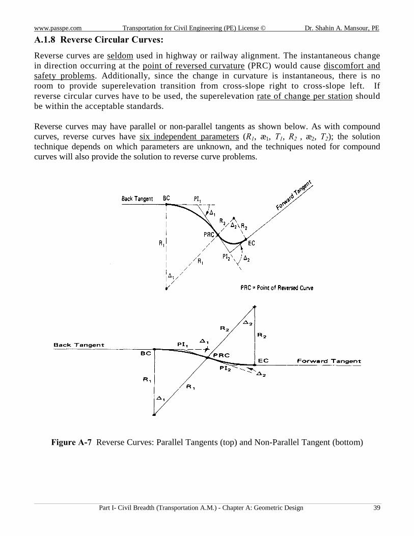
A.1.8 Reverse Circular Curves:
Reverse curves are seldom used in highway or railway alignment. The instantaneous change in direction occurring at the point of reversed curvature (PRC) would cause discomfort and safety problems. Additionally, since the change in curvature is instantaneous, there is no room to provide superelevation transition from cross-slope right to cross-slope left. If reverse circular curves have to be used, the superelevation rate of change per station should be within the acceptable standards.
Reverse curves may have parallel or non-parallel tangents as shown below. As with compound curves, reverse curves have six independent parameters (R1, ∆1, T1, R2 , ∆2, T2); the solution technique depends on which parameters are unknown, and the techniques noted for compound curves will also provide the solution to reverse curve problems.
Figure A-7 Reverse Curves: Parallel Tangents (top) and Non-Parallel Tangent (bottom)
www.passpe.com Transportation for Civil PE License © Dr. Shahin A.Mansour, PE
Part I- Civil Breadth (Transportation A.M.) - Chapter A: Geometric Design 40
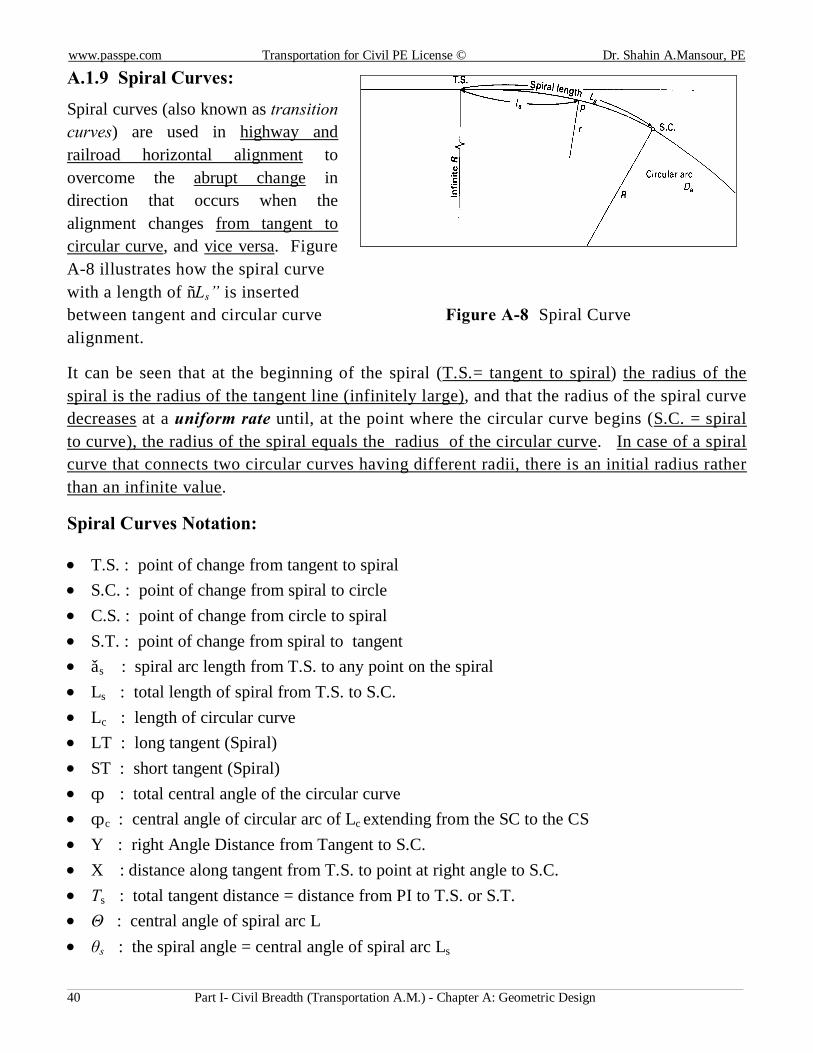
A.1.9 Spiral Curves:
Spiral curves (also known as transition curves) are used in highway and railroad horizontal alignment to overcome the abrupt change in direction that occurs when the alignment changes from tangent to circular curve, and vice versa. Figure A-8 illustrates how the spiral curve with a length of “Ls” is inserted between tangent and circular curve Figure A-8 Spiral Curve alignment.
It can be seen that at the beginning of the spiral (T.S.= tangent to spiral) the radius of the spiral is the radius of the tangent line (infinitely large), and that the radius of the spiral curve decreases at a uniform rate until, at the point where the circular curve begins (S.C. = spiral to curve), the radius of the spiral equals the radius of the circular curve. In case of a spiral curve that connects two circular curves having different radii, there is an initial radius rather than an infinite value.
Spiral Curves Notation:
• T.S. : point of change from tangent to spiral • S.C. : point of change from spiral to circle • C.S. : point of change from circle to spiral • S.T. : point of change from spiral to tangent • ℓs : spiral arc length from T.S. to any point on the spiral • Ls : total length of spiral from T.S. to S.C. • Lc : length of circular curve • LT : long tangent (Spiral) • ST : short tangent (Spiral) • Δ : total central angle of the circular curve • Δ c : central angle of circular arc of Lc extending from the SC to the CS • Y : right Angle Distance from Tangent to S.C. • X : distance along tangent from T.S. to point at right angle to S.C. • Ts : total tangent distance = distance from PI to T.S. or S.T. • Θ : central angle of spiral arc L • θs : the spiral angle = central angle of spiral arc Ls

www.passpe.com Transportation for Civil Engineering (PE) License © Dr. Shahin A. Mansour, PE
Part I- Civil Breadth (Transportation A.M.) - Chapter A: Geometric Design 41
Figure A-9 Spiral Curve
www.passpe.com Transportation for Civil PE License © Dr. Shahin A.Mansour, PE
Part I- Civil Breadth (Transportation A.M.) - Chapter A: Geometric Design 42
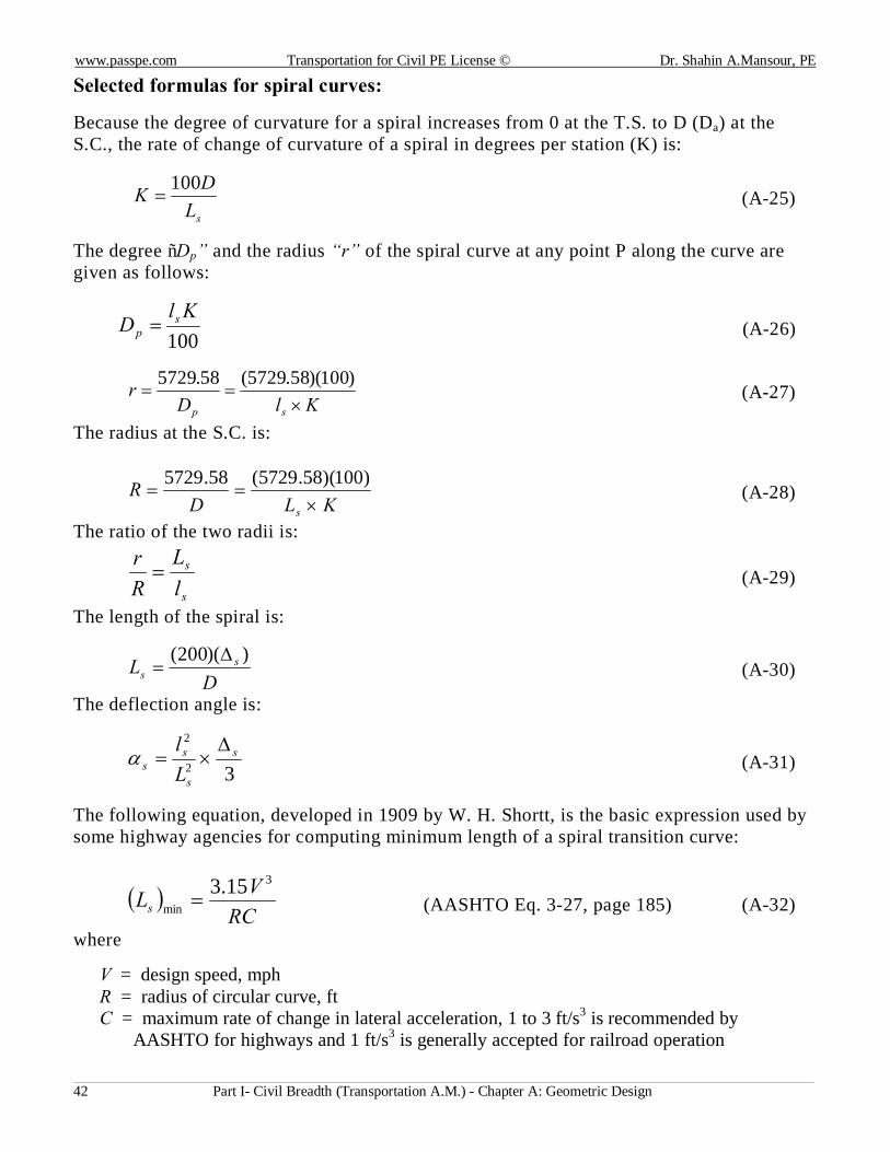
Selected formulas for spiral curves: Because the degree of curvature for a spiral increases from 0 at the T.S. to D (Da) at the S.C., the rate of change of curvature of a spiral in degrees per station (K) is:
sLDK 100
= (A-25)
The degree “Dp” and the radius “r” of the spiral curve at any point P along the curve are given as follows:
100Kl
D sp = (A-26)
KlD
rsp ×
==)100)(58.5729(58.5729
(A-27)
The radius at the S.C. is:
KLDR
s ×==
)100)(58.5729(58.5729 (A-28)
The ratio of the two radii is:
s
s
lL
Rr
= (A-29)
The length of the spiral is:
DL s
s))(200( ∆
= (A-30)
The deflection angle is:
32
2s
s
ss L
l ∆×=α (A-31)
The following equation, developed in 1909 by W. H. Shortt, is the basic expression used by some highway agencies for computing minimum length of a spiral transition curve:
( )RC
VLs
3
min15.3
= (AASHTO Eq. 3-27, page 185) (A-32)
where
V = design speed, mph R = radius of circular curve, ft C = maximum rate of change in lateral acceleration, 1 to 3 ft/s3 is recommended by AASHTO for highways and 1 ft/s3 is generally accepted for railroad operation
www.passpe.com Transportation for Civil Engineering (PE) License © Dr. Shahin A. Mansour, PE
Part I- Civil Breadth (Transportation A.M.) - Chapter A: Geometric Design 43
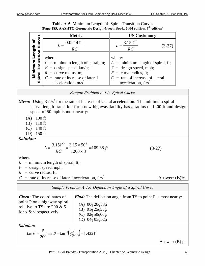
Table A-5 Minimum Length of Spiral Transition Curves (Page 185, AASHTO Geometric Design-Green Book, 2004 edition, 5th edition)
M
inim
um L
engt
h of
S
pira
l Tra
nsit
ion
Cur
ves Metric US Customary
RCVL
30214.0=
RCVL
315.3= (3-27)
where: L = minimum length of spiral, m; V = design speed, km/h; R = curve radius, m; C = rate of increase of lateral acceleration, m/s3
where: L = minimum length of spiral, ft; V = design speed, mph; R = curve radius, ft; C = rate of increase of lateral acceleration, ft/s3
Sample Problem A-14: Spiral Curve
Given: Using 3 ft/s3 for the rate of increase of lateral acceleration. The minimum spiral curve length transition for a new highway facility has a radius of 1200 ft and design
speed of 50 mph is most nearly:
(A) 100 ft (B) 110 ft (C) 140 ft (D) 150 ft
Solution:
ftRC
VL 38.10931200
5015.315.3 33
=×
×== (3-27)
where: L = minimum length of spiral, ft; V = design speed, mph; R = curve radius, ft; C = rate of increase of lateral acceleration, ft/s3 Answer: (B)◄
Sample Problem A-15: Deflection Angle of a Spiral Curve
Given: The coordinates of point P on a highway spiral relative to TS are 200 & 5 for x & y respectively.
Find: The deflection angle from TS to point P is most nearly:
(A) 00˚ 28ʹ 38ʺ (B) 01˚ 25ʹ 55ʺ (C) 02˚ 50ʹ 00ʺ (D) 04˚ 05ʹ 02ʺ
Solution:
( ) o4321.12005tan
2005tan 1 ==⇒= −θθ
Answer: (B) ◄
www.passpe.com Transportation for Civil PE License © Dr. Shahin A.Mansour, PE
Part I- Civil Breadth (Transportation A.M.) - Chapter A: Geometric Design 44
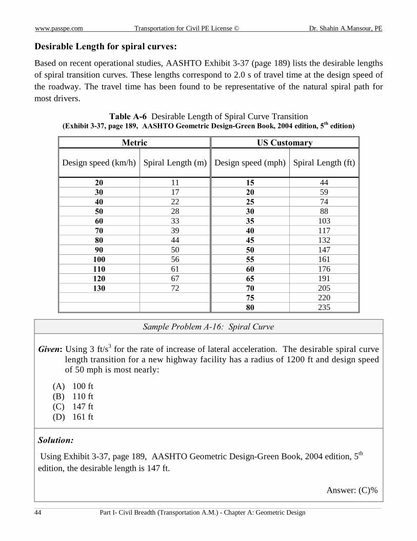
Desirable Length for spiral curves:
Based on recent operational studies, AASHTO Exhibit 3-37 (page 189) lists the desirable lengths of spiral transition curves. These lengths correspond to 2.0 s of travel time at the design speed of the roadway. The travel time has been found to be representative of the natural spiral path for most drivers.
Table A-6 Desirable Length of Spiral Curve Transition (Exhibit 3-37, page 189, AASHTO Geometric Design-Green Book, 2004 edition, 5th edition)
Metric US Customary
Design speed (km/h) Spiral Length (m) Design speed (mph) Spiral Length (ft)
20 11 15 44 30 17 20 59 40 22 25 74 50 28 30 88 60 33 35 103 70 39 40 117 80 44 45 132 90 50 50 147 100 56 55 161 110 61 60 176 120 67 65 191 130 72 70 205
75 220 80 235
Sample Problem A-16: Spiral Curve Given: Using 3 ft/s3 for the rate of increase of lateral acceleration. The desirable spiral curve
length transition for a new highway facility has a radius of 1200 ft and design speed of 50 mph is most nearly:
(A) 100 ft (B) 110 ft (C) 147 ft (D) 161 ft
Solution:
Using Exhibit 3-37, page 189, AASHTO Geometric Design-Green Book, 2004 edition, 5th edition, the desirable length is 147 ft.
Answer: (C)◄
www.passpe.com Transportation for Civil Engineering (PE) License © Dr. Shahin A. Mansour, PE
Part I- Civil Breadth (Transportation A.M.) - Chapter A: Geometric Design 45
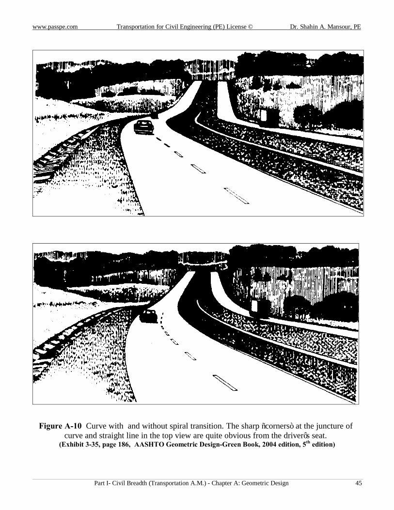
Figure A-10 Curve with and without spiral transition. The sharp “corners” at the juncture of
curve and straight line in the top view are quite obvious from the driver’s seat. (Exhibit 3-35, page 186, AASHTO Geometric Design-Green Book, 2004 edition, 5th edition)
www.passpe.com Transportation for Civil PE License © Dr. Shahin A.Mansour, PE
Part I- Civil Breadth (Transportation A.M.) - Chapter A: Geometric Design 46
A.2 VERTICAL CURVES
A.2.1 Why Vertical Curves are Used?
Roads made up of a series of straight lines (or tangents) are not practical. To prevent abrupt changes in the vertical direction of moving vehicles, adjacent segments of differing grade are connected by a curve. This curve in the vertical plane is called a vertical curve.
The geometric curve used in vertical alignment design is the parabola curve. The parabola has these two desirable characteristics of:
(1) a constant rate of change of grade (L
ggr 12 −= ), which contributes to smooth
alignment transition, and
(2) ease of computation of vertical offsets, which permits easily computed curve eleva-tions.
As a general rule, the higher the speed the road is designed for, the smaller the percent of grade that is allowed. For example, a road designed for a maximum speed of 30 miles per hour (mph) may have a vertical curve with the tangents to the curve arc having a grade as high as 6 to 8 percent. A road that is designed for 70 mph can have a vertical curve whose tangents have a grade of only 3 to 5 percent.
A.2.2 Vertical Curves Terminology:
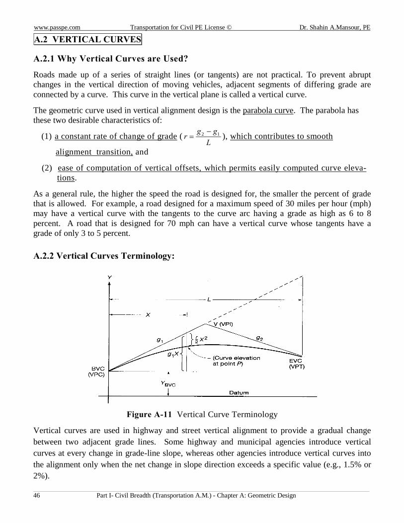
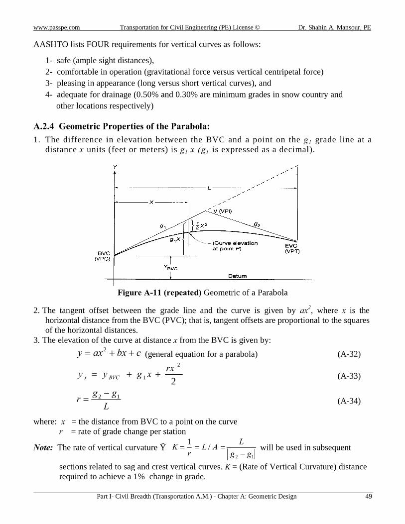
Figure A-11 Vertical Curve Terminology
Vertical curves are used in highway and street vertical alignment to provide a gradual change between two adjacent grade lines. Some highway and municipal agencies introduce vertical curves at every change in grade-line slope, whereas other agencies introduce vertical curves into the alignment only when the net change in slope direction exceeds a specific value (e.g., 1.5% or 2%).
www.passpe.com Transportation for Civil Engineering (PE) License © Dr. Shahin A. Mansour, PE
Part I- Civil Breadth (Transportation A.M.) - Chapter A: Geometric Design 47
In Figure A-11, vertical curve terminology is introduced: g1 is the slope (percent) of the entering grade line, g2 is the slope of the exiting grade line, BVC is the beginning of the vertical curve, EVC is the end of the vertical curve, and PVI is the point of intersection of the two adjacent grade lines. The length of vertical curve ( L ) is the projection of the curve onto a horizontal surface and as such corresponds to plan distance.
A.2.3 Types of Vertical Curves:
Vertical curves may be classified based on the location of the vertex with respect to the BVC and EVC as symmetrical and asymmetrical.
Table A-7 Types of Vertical Curves
Symmetrical Vertical Curves Asymmetrical Vertical Curves Ø The vertex is located at the half distance
between the BVC & EVC. Ø The equations used to solve the unknowns
are based on parabolic formula. Ø They are used mostly in every project
where no minimum vertical clearance or cover is needed.
Ø They are also called equal-tangent parabolic vertical curves.
Ø The vertex is not located at the half distance
between the BVC & EVC. Ø The equations used to solve the unknowns
are based on parabolic formula (two vertical curves).
Ø They used when a specific elevation at a certain station (point) is required and the grades of the grade lines are fixed.
Ø They are also called unequal-tangent parabolic vertical curves.
Another classification is crest and sag vertical curves.
Table A-8 Types of Vertical Curves
Sag Vertical Curves (g2 > g1) Crest Vertical Curves (g2 < g1) Ø They can be symmetrical or
asymmetrical. Ø The equation used to solve the unknowns
is a parabolic formula. Ø They connect downgrade (–) tangent to
an upgrade (+) tangent (type III). Ø The rate of grade change per station
Lggr 12 −
= is a positive quantity.
Ø They can be symmetrical or asymmetrical.
Ø The equation used to solve the unknowns
is a parabolic formula. Ø They connect an upgrade (+) tangent to a
downgrade (–) tangent (type I). Ø The rate of grade change per station
Lggr 12 −
= is a negative quantity.
www.passpe.com Transportation for Civil PE License © Dr. Shahin A.Mansour, PE
Part I- Civil Breadth (Transportation A.M.) - Chapter A: Geometric Design 48
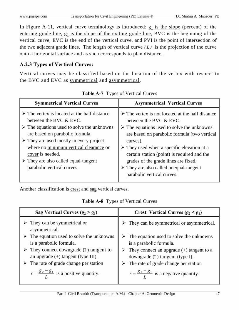
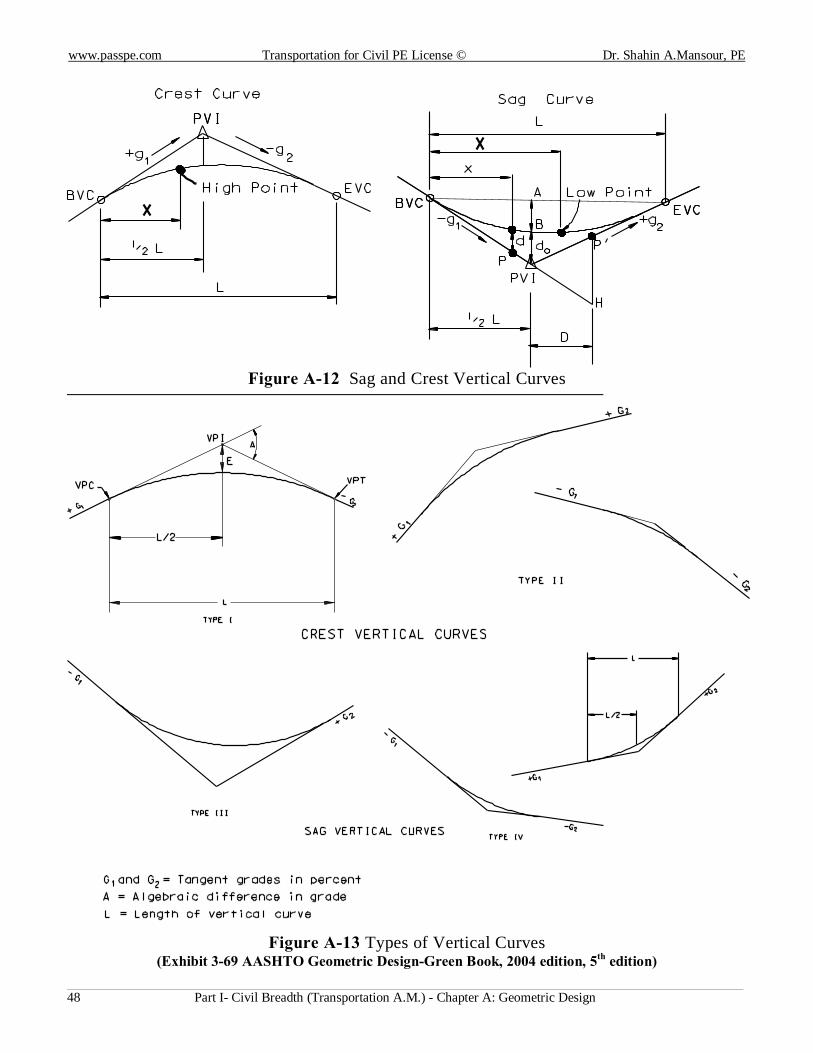
Figure A-12 Sag and Crest Vertical Curves
Figure A-13 Types of Vertical Curves (Exhibit 3-69 AASHTO Geometric Design-Green Book, 2004 edition, 5th edition)
www.passpe.com Transportation for Civil Engineering (PE) License © Dr. Shahin A. Mansour, PE
Part I- Civil Breadth (Transportation A.M.) - Chapter A: Geometric Design 49
AASHTO lists FOUR requirements for vertical curves as follows:
1- safe (ample sight distances), 2- comfortable in operation (gravitational force versus vertical centripetal force) 3- pleasing in appearance (long versus short vertical curves), and 4- adequate for drainage (0.50% and 0.30% are minimum grades in snow country and other locations respectively)
A.2.4 Geometric Properties of the Parabola: 1. The difference in elevation between the BVC and a point on the g1 grade line at a
distance x units (feet or meters) is g1 x (g1 is expressed as a decimal).
Figure A-11 (repeated) Geometric of a Parabola
2. The tangent offset between the grade line and the curve is given by ax2, where x is the horizontal distance from the BVC (PVC); that is, tangent offsets are proportional to the squares of the horizontal distances.
3. The elevation of the curve at distance x from the BVC is given by: cbxaxy ++= 2 (general equation for a parabola) (A-32)
2
2
1rxxgyy BVCx ++= (A-33)
Lggr 12 −
= (A-34) where: x = the distance from BVC to a point on the curve r = rate of grade change per station
Note: The rate of vertical curvature → 12
/1gg
LALr
K−
=== will be used in subsequent
sections related to sag and crest vertical curves. K = (Rate of Vertical Curvature) distance required to achieve a 1% change in grade.
www.passpe.com Transportation for Civil PE License © Dr. Shahin A.Mansour, PE
Part I- Civil Breadth (Transportation A.M.) - Chapter A: Geometric Design 50
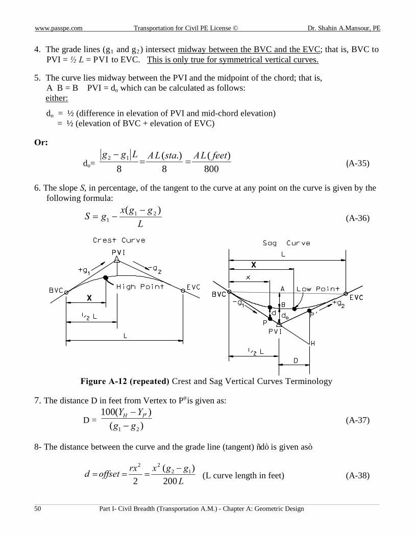
4. The grade lines (g1 and g2) intersect midway between the BVC and the EVC; that is, BVC to
PVI = ½ L = PVI to EVC. This is only true for symmetrical vertical curves.
5. The curve lies midway between the PVI and the midpoint of the chord; that is, A‒B = B ‒ PVI = do which can be calculated as follows:
either:
do = ½ (difference in elevation of PVI and mid-chord elevation) = ½ (elevation of BVC + elevation of EVC)
Or:
do= 800)(
8.)(
812 feetLAstaLALgg
==−
(A-35)
6. The slope S, in percentage, of the tangent to the curve at any point on the curve is given by the following formula:
LggxgS )( 21
1−
−= (A-36)
Figure A-12 (repeated) Crest and Sag Vertical Curves Terminology
7. The distance D in feet from Vertex to Pʹ is given as:
D = )()(100
21 ggYY PH
−− ′
(A-37)
8- The distance between the curve and the grade line (tangent) “d” is given as”
Lggxrxoffsetd
200)(
212
22 −=== (L curve length in feet) (A-38)
www.passpe.com Transportation for Civil Engineering (PE) License © Dr. Shahin A. Mansour, PE
Part I- Civil Breadth (Transportation A.M.) - Chapter A: Geometric Design 51
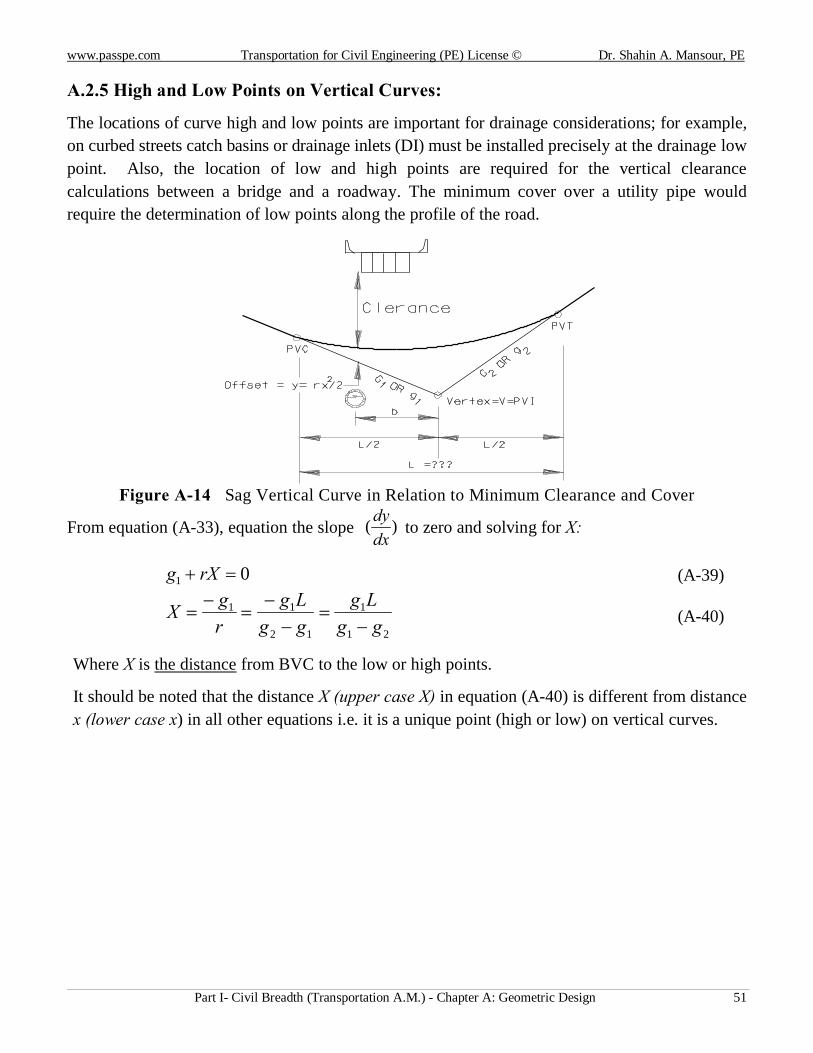
A.2.5 High and Low Points on Vertical Curves:
The locations of curve high and low points are important for drainage considerations; for example, on curbed streets catch basins or drainage inlets (DI) must be installed precisely at the drainage low point. Also, the location of low and high points are required for the vertical clearance calculations between a bridge and a roadway. The minimum cover over a utility pipe would require the determination of low points along the profile of the road.
Figure A-14 Sag Vertical Curve in Relation to Minimum Clearance and Cover
From equation (A-33), equation the slope )(dxdy
to zero and solving for X:
01 =+ rXg (A-39)
21
1
12
11
ggLg
ggLg
rgX
−=
−−
=−
= (A-40)
Where X is the distance from BVC to the low or high points.
It should be noted that the distance X (upper case X) in equation (A-40) is different from distance x (lower case x) in all other equations i.e. it is a unique point (high or low) on vertical curves.
www.passpe.com Transportation for Civil PE License © Dr. Shahin A.Mansour, PE
Part I- Civil Breadth (Transportation A.M.) - Chapter A: Geometric Design 52
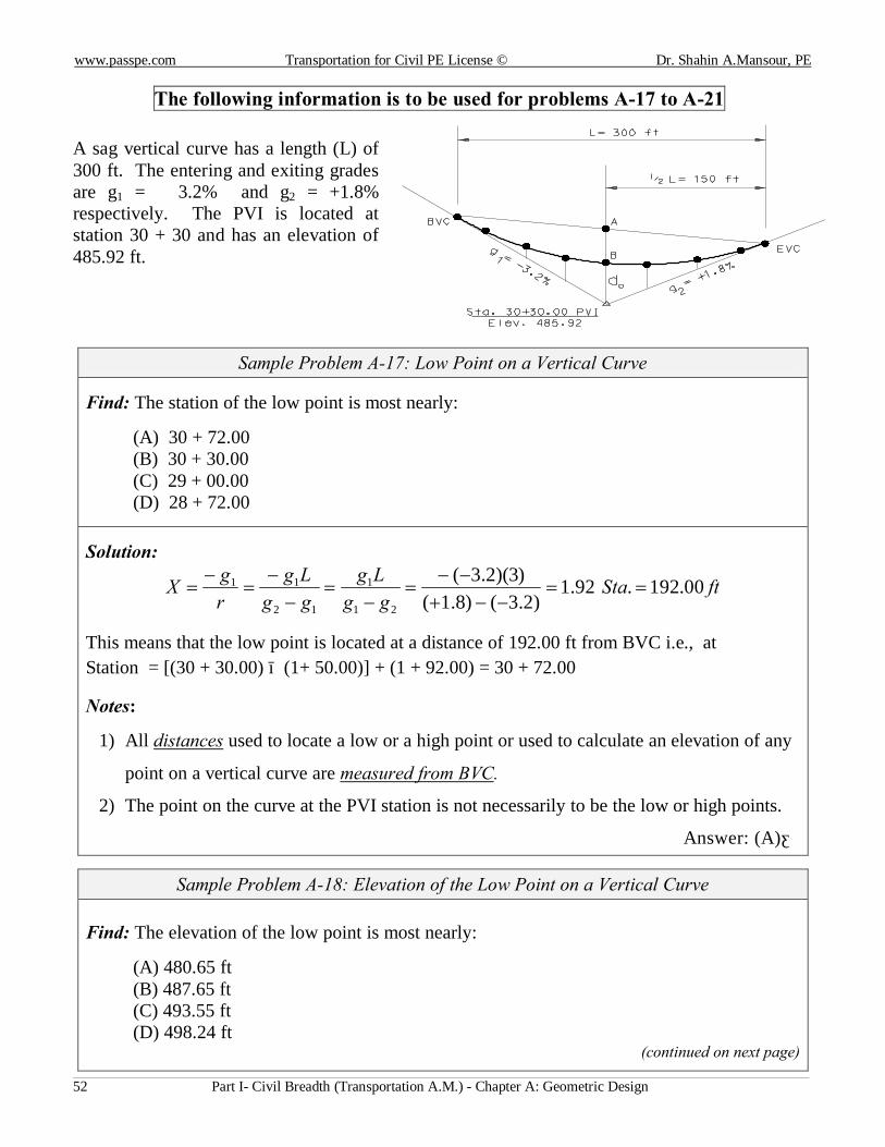
The following information is to be used for problems A-17 to A-21
A sag vertical curve has a length (L) of 300 ft. The entering and exiting grades are g1 = ‒ 3.2% and g2 = +1.8% respectively. The PVI is located at station 30 + 30 and has an elevation of 485.92 ft.
Sample Problem A-17: Low Point on a Vertical Curve
Find: The station of the low point is most nearly:
(A) 30 + 72.00 (B) 30 + 30.00 (C) 29 + 00.00 (D) 28 + 72.00
Solution:
ftStagg
LgggLg
rgX 00.192.92.1
)2.3()8.1()3)(2.3(
21
1
12
11 ==−−+
−−=
−=
−−
=−
=
This means that the low point is located at a distance of 192.00 ft from BVC i.e., at Station = [(30 + 30.00) − (1+ 50.00)] + (1 + 92.00) = 30 + 72.00
Notes:
1) All distances used to locate a low or a high point or used to calculate an elevation of any
point on a vertical curve are measured from BVC.
2) The point on the curve at the PVI station is not necessarily to be the low or high points.
Answer: (A)◄
Sample Problem A-18: Elevation of the Low Point on a Vertical Curve Find: The elevation of the low point is most nearly:
(A) 480.65 ft (B) 487.65 ft (C) 493.55 ft (D) 498.24 ft
(continued on next page)
www.passpe.com Transportation for Civil Engineering (PE) License © Dr. Shahin A. Mansour, PE
Part I- Civil Breadth (Transportation A.M.) - Chapter A: Geometric Design 53
Solution:
2
2
1rxxgyy BVCx ++=
[ ] [email protected])292.1)(
00.3)2.3(8.1()92.1)(2.3()2.3)(5.1(92.485
2
+=−−
+−++= Staft
Answer: (B)◄
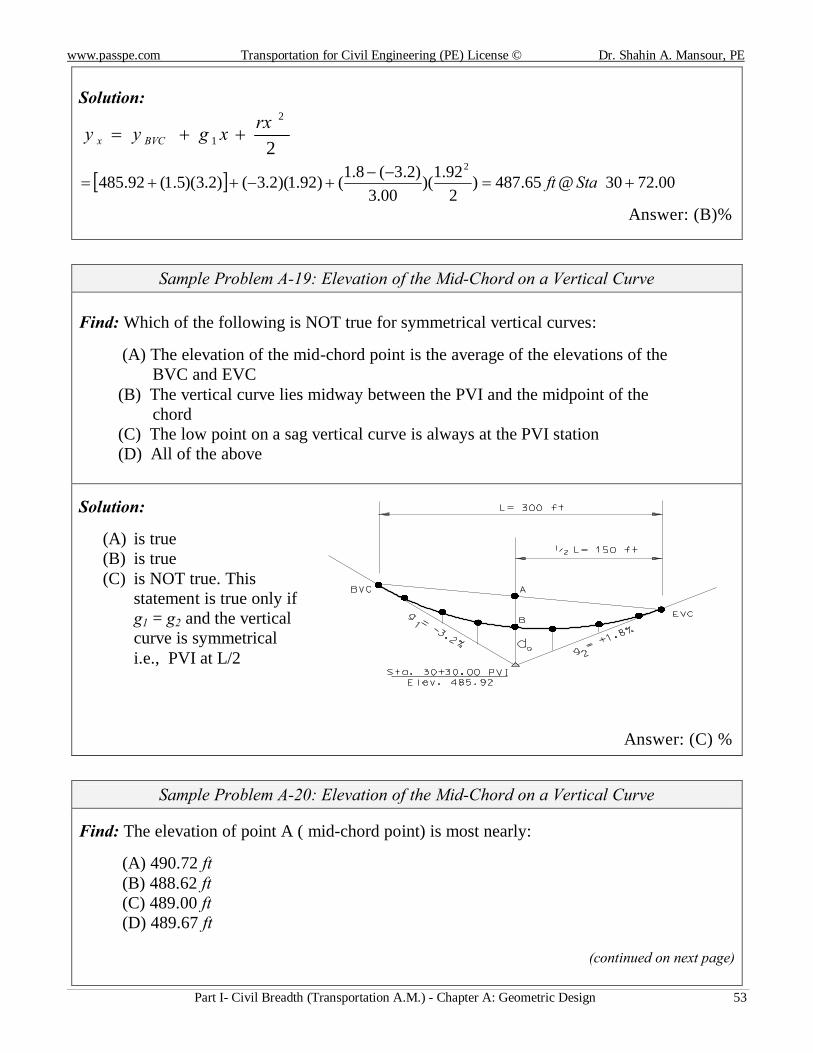
Sample Problem A-19: Elevation of the Mid-Chord on a Vertical Curve Find: Which of the following is NOT true for symmetrical vertical curves:
(A) The elevation of the mid-chord point is the average of the elevations of the BVC and EVC (B) The vertical curve lies midway between the PVI and the midpoint of the chord (C) The low point on a sag vertical curve is always at the PVI station (D) All of the above
Solution:
(A) is true (B) is true (C) is NOT true. This
statement is true only if g1 = g2 and the vertical curve is symmetrical i.e., PVI at L/2
Answer: (C) ◄
Sample Problem A-20: Elevation of the Mid-Chord on a Vertical Curve
Find: The elevation of point A ( mid-chord point) is most nearly:
(A) 490.72 ft (B) 488.62 ft (C) 489.00 ft (D) 489.67 ft
(continued on next page)
www.passpe.com Transportation for Civil PE License © Dr. Shahin A.Mansour, PE
Part I- Civil Breadth (Transportation A.M.) - Chapter A: Geometric Design 54
Solution:
mid-chord elevation (point A) = ½ (Elevation of BVC + Elevation of EVC)
= ½ {(485.92 + 1.5 ×3.2) + (485.92 +1.5 × 1.8)}= 489.67 ft
Answer: (D)◄
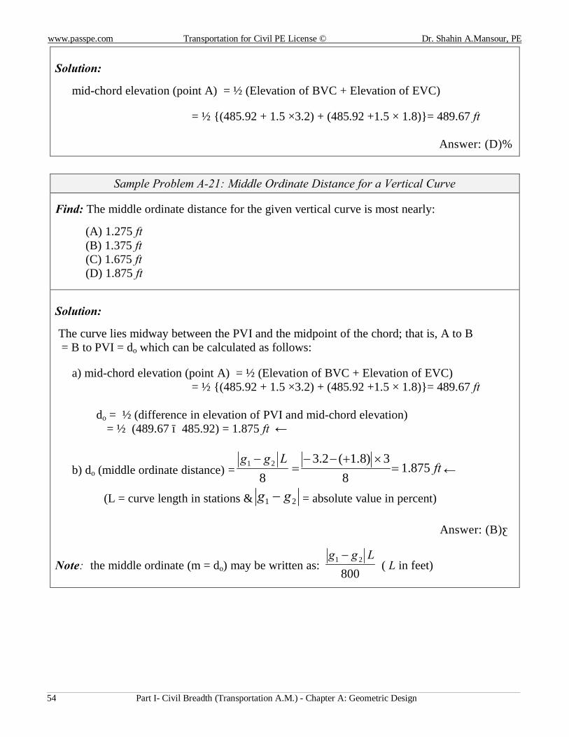
Sample Problem A-21: Middle Ordinate Distance for a Vertical Curve
Find: The middle ordinate distance for the given vertical curve is most nearly:
(A) 1.275 ft (B) 1.375 ft (C) 1.675 ft (D) 1.875 ft
Solution:
The curve lies midway between the PVI and the midpoint of the chord; that is, A to B = B to PVI = do which can be calculated as follows:
a) mid-chord elevation (point A) = ½ (Elevation of BVC + Elevation of EVC) = ½ {(485.92 + 1.5 ×3.2) + (485.92 +1.5 × 1.8)}= 489.67 ft
do = ½ (difference in elevation of PVI and mid-chord elevation)
= ½ (489.67 − 485.92) = 1.875 ft ←
b) do (middle ordinate distance) = ftLgg
875.18
3)8.1(2.38
21 =×+−−
=−
←
(L = curve length in stations & 21 gg − = absolute value in percent)
Answer: (B)◄
Note: the middle ordinate (m = do) may be written as: 800
21 Lgg −( L in feet)

www.passpe.com Transportation for Civil Engineering (PE) License © Dr. Shahin A. Mansour, PE
Part I- Civil Breadth (Transportation A.M.) - Chapter A: Geometric Design 55
A.2.7 Asymmetrical (Unsymmetrical) Vertical Curves:
Asymmetrical vertical curves; also called unequal tangent vertical curves, are encountered in practice where certain limitations are exist as fixed tangent grades, vertical clearance or minimum cover. The vertex for unequal tangent curve is not in the middle between the BVC and EVC. An unequal tangent vertical curve is simply a pair of equal tangent curves, where the EVC of the first is the BVC of the second. This point is called CVC, point of compound vertical curvature. The same basic equation for the symmetrical curves will be used for the unsymmetrical curves.
Figure A-15 Unsymmetrical Vertical Curve
Sample Problem A-22: Unsymmetrical Vertical Curve Given: g1 = – 2 %, g2 = +1.6 %,, BCV, V and EVC stations are 83 + 00, 87 + 00 and 93 + 00 respectively. Elevation at V = 743.24 ft. See Figure A.17
Find: Elevations, first & second difference at full stations
Solution:
The following steps will be followed:
Step 1: YBVC = 743.24 + 4(2.00) = 751.24 ft YA = 743.24 + 2(2.00) = 747.24 ft YEVC = 743.24 + 6 (1.60) = 752.84 ft YB = 743.24 + 3(1.60) = 748.04 ft
(Grade)AB = %16.05
24.74704.748+=
−
YCVC = 747.24 + 2(0.16) = 747.56 ft Step 2:
star /%54.04
)00.2(16.01 +=
−−= & star /%24.0
616.060.1
2 +=−
=
(continued on next page)
www.passpe.com Transportation for Civil PE License © Dr. Shahin A.Mansour, PE
Part I- Civil Breadth (Transportation A.M.) - Chapter A: Geometric Design 56
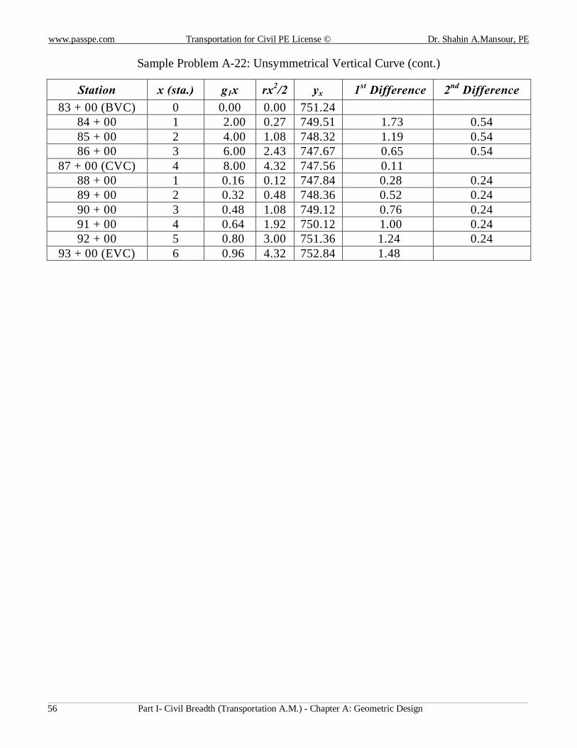
Sample Problem A-22: Unsymmetrical Vertical Curve (cont.)
Station x (sta.) g1x rx2/2 yx 1st Difference 2nd Difference 83 + 00 (BVC) 0 0.00 0.00 751.24
84 + 00 1 ‒ 2.00 0.27 749.51 ‒ 1.73 0.54 85 + 00 2 ‒ 4.00 1.08 748.32 ‒ 1.19 0.54 86 + 00 3 ‒ 6.00 2.43 747.67 ‒ 0.65 0.54
87 + 00 (CVC) 4 ‒ 8.00 4.32 747.56 ‒ 0.11 88 + 00 1 0.16 0.12 747.84 0.28 0.24 89 + 00 2 0.32 0.48 748.36 0.52 0.24 90 + 00 3 0.48 1.08 749.12 0.76 0.24 91 + 00 4 0.64 1.92 750.12 1.00 0.24 92 + 00 5 0.80 3.00 751.36 1.24 0.24
93 + 00 (EVC) 6 0.96 4.32 752.84 1.48
www.passpe.com Transportation for Civil Engineering (PE) License © Dr. Shahin A. Mansour, PE
Part I- Civil Breadth (Transportation A.M.) - Chapter A: Geometric Design 57
A.3 SIGHT DISTANCES
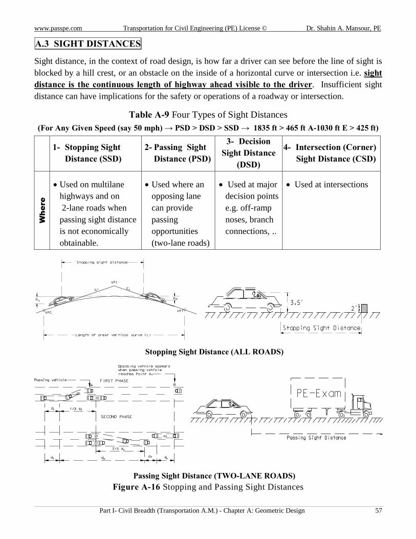
Sight distance, in the context of road design, is how far a driver can see before the line of sight is blocked by a hill crest, or an obstacle on the inside of a horizontal curve or intersection i.e. sight distance is the continuous length of highway ahead visible to the driver. Insufficient sight distance can have implications for the safety or operations of a roadway or intersection.
Table A-9 Four Types of Sight Distances
(For Any Given Speed (say 50 mph) → PSD > DSD > SSD → 1835 ft > 465 ft A-1030 ft E > 425 ft)
1- Stopping Sight
Distance (SSD) 2- Passing Sight
Distance (PSD)
3- Decision Sight Distance
(DSD)
4- Intersection (Corner) Sight Distance (CSD)
Whe
re
• Used on multilane highways and on 2-lane roads when passing sight distance is not economically obtainable.
• Used where an opposing lane can provide passing opportunities (two-lane roads)
• Used at major decision points e.g. off-ramp noses, branch connections, ..
• Used at intersections
Stopping Sight Distance (ALL ROADS)
Passing Sight Distance (TWO-LANE ROADS) Figure A-16 Stopping and Passing Sight Distances
www.passpe.com Transportation for Civil PE License © Dr. Shahin A.Mansour, PE
Part I- Civil Breadth (Transportation A.M.) - Chapter A: Geometric Design 58
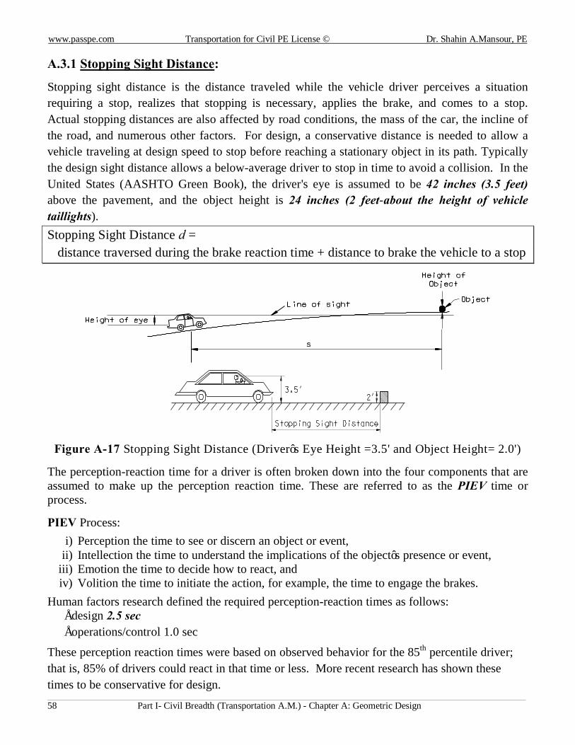
A.3.1 Stopping Sight Distance:
Stopping sight distance is the distance traveled while the vehicle driver perceives a situation requiring a stop, realizes that stopping is necessary, applies the brake, and comes to a stop. Actual stopping distances are also affected by road conditions, the mass of the car, the incline of the road, and numerous other factors. For design, a conservative distance is needed to allow a vehicle traveling at design speed to stop before reaching a stationary object in its path. Typically the design sight distance allows a below-average driver to stop in time to avoid a collision. In the United States (AASHTO Green Book), the driver's eye is assumed to be 42 inches (3.5 feet) above the pavement, and the object height is 24 inches (2 feet-about the height of vehicle taillights). Stopping Sight Distance d = distance traversed during the brake reaction time + distance to brake the vehicle to a stop
Figure A-17 Stopping Sight Distance (Driver’s Eye Height =3.5' and Object Height= 2.0')
The perception-reaction time for a driver is often broken down into the four components that are assumed to make up the perception reaction time. These are referred to as the PIEV time or process.
PIEV Process:
i) Perception the time to see or discern an object or event, ii) Intellection the time to understand the implications of the object’s presence or event,
iii) Emotion the time to decide how to react, and iv) Volition the time to initiate the action, for example, the time to engage the brakes.
Human factors research defined the required perception-reaction times as follows:
• design 2.5 sec • operations/control 1.0 sec
These perception reaction times were based on observed behavior for the 85th percentile driver; that is, 85% of drivers could react in that time or less. More recent research has shown these times to be conservative for design.

www.passpe.com Transportation for Civil Engineering (PE) License © Dr. Shahin A. Mansour, PE
Part I- Civil Breadth (Transportation A.M.) - Chapter A: Geometric Design 59
A.3.1.1 Stopping Sight Distance On A Flat Grade:
The following equations will be used to calculate the stopping distance on a flat grade facilities:
Table A-10 Stopping Sight Distance Equations on Flat Grades (Page 113- AASHTO Geometric Design-Green Book, 2004 edition, 5th edition)
Sto
ppin
g S
ight
D
ista
nce
(SS
D)
Metric US Customary
aVVtd
2
039.0278.0 += a
VVtd2
075.147.1 += (3-2)
where: t = brake reaction time, 2.5 s; V = design speed, km/h; a = deceleration rate, m/s2 (3.4 m/s2)
where: t = brake reaction time, 2.5 s; V = design speed, mph; a = deceleration rate, ft/s2 (11.2 ft/s2)
The above equations are used to generate the following table for wet-pavement conditions.
Table A-11 Stopping Sight Distance on Flat Grades (Exhibit 3-1, page 112, AASHTO Geometric Design-Green Book, 2004 edition, 5th edition)
Metric US Customary
Design speed
(km/h)
Brake reaction distance
(m)
Braking distance on level
(m)
Stopping sight distance Design
speed (mph)
Brake reaction distance
(ft)
Braking distance on level
(ft)
Stopping sight distance
Calculated (m)
Design (m)
Calculated (ft)
Design (ft)
20 13.9 4.6 18.5 20 15 55.1 21.6 76.7 80 30 20.9 10.3 31.2 35 20 73.5 38.4 111.9 115 40 27.8 18.4 46.2 50 25 91.9 60.0 151.9 155 50 34.8 28.7 63.5 65 30 110.3 86.4 196.7 200 60 41.7 41.3 83.0 85 35 128.6 117.6 246.2 250 70 48.7 56.2 104.9 105 40 147.0 153.6 300.6 305 80 55.6 73.4 129.0 130 45 165.4 194.4 359.8 360 90 62.6 92.9 155.5 160 50 183.8 240.0 423.8 425
100 69.5 114.7 184.2 185 55 202.1 290.3 492.4 495 110 76.5 138.8 215.3 220 60 220.5 345.5 566.0 570 120 83.4 165.2 248.6 250 65 238.9 405.5 644.4 645 130 90.4 193.8 284.2 285 70 257.3 470.3 727.6 730
75 275.6 539.9 815.5 820 80 294.0 614.3 908.3 910
Note: Brake reaction distance predicated on a time of 2.5 s; deceleration rate of 3.4 m/s2 [11.2 ft/s2] used to
determine calculated sight distance.
www.passpe.com Transportation for Civil PE License © Dr. Shahin A.Mansour, PE
Part I- Civil Breadth (Transportation A.M.) - Chapter A: Geometric Design 60
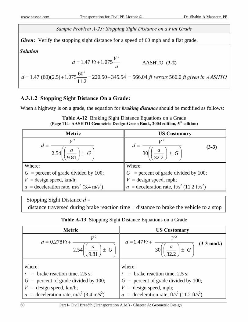
Sample Problem A-23: Stopping Sight Distance on a Flat Grade
Given: Verify the stopping sight distance for a speed of 60 mph and a flat grade.
Solution
aVVtd
2
075.147.1 += AASHTO (3-2)
AASHTOingivenftversusftd 0.56604.56654.34550.2202.11
60075.1)5.2)(60(47.12
=+=+=
A.3.1.2 Stopping Sight Distance On a Grade:
When a highway is on a grade, the equation for braking distance should be modified as follows:
Table A-12 Braking Sight Distance Equations on a Grade (Page 114- AASHTO Geometric Design-Green Book, 2004 edition, 5th edition)
Metric US Customary
±
=Ga
Vd
81.954.2
2
±
=Ga
Vd
2.3230
2
(3-3)
Where: G = percent of grade divided by 100; V = design speed, km/h; a = deceleration rate, m/s2 (3.4 m/s2)
Where: G = percent of grade divided by 100; V = design speed, mph; a = deceleration rate, ft/s2 (11.2 ft/s2)
Stopping Sight Distance d = distance traversed during brake reaction time + distance to brake the vehicle to a stop
Table A-13 Stopping Sight Distance Equations on a Grade
Metric US Customary
±
+=Ga
VVtd
81.954.2
278.02
±
+=Ga
VVtd
2.3230
47.12
(3-3 mod.)
where: t = brake reaction time, 2.5 s; G = percent of grade divided by 100; V = design speed, km/h; a = deceleration rate, m/s2 (3.4 m/s2)
where: t = brake reaction time, 2.5 s; G = percent of grade divided by 100; V = design speed, mph; a = deceleration rate, ft/s2 (11.2 ft/s2)
www.passpe.com Transportation for Civil Engineering (PE) License © Dr. Shahin A. Mansour, PE
Part I- Civil Breadth (Transportation A.M.) - Chapter A: Geometric Design 61
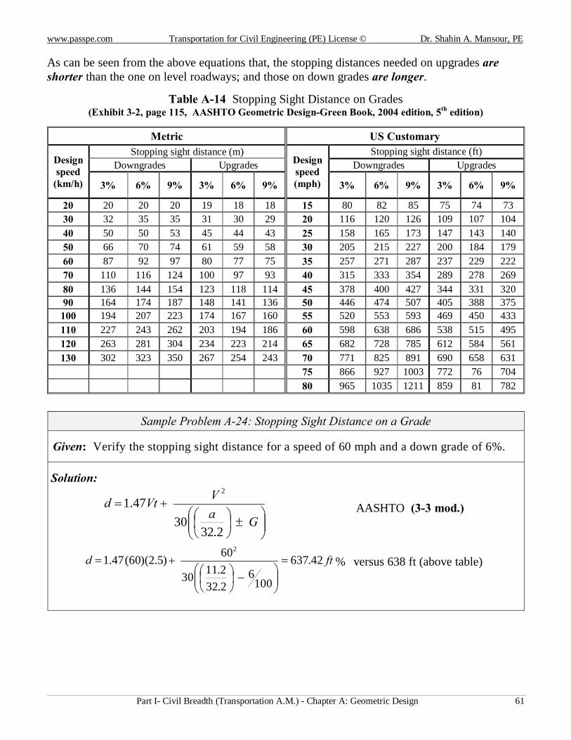
As can be seen from the above equations that, the stopping distances needed on upgrades are shorter than the one on level roadways; and those on down grades are longer.
Table A-14 Stopping Sight Distance on Grades (Exhibit 3-2, page 115, AASHTO Geometric Design-Green Book, 2004 edition, 5th edition)
Metric US Customary
Design speed
(km/h)
Stopping sight distance (m) Design speed (mph)
Stopping sight distance (ft) Downgrades Upgrades Downgrades Upgrades
3% 6% 9% 3% 6% 9% 3% 6% 9% 3% 6% 9%
20 20 20 20 19 18 18 15 80 82 85 75 74 73 30 32 35 35 31 30 29 20 116 120 126 109 107 104 40 50 50 53 45 44 43 25 158 165 173 147 143 140 50 66 70 74 61 59 58 30 205 215 227 200 184 179 60 87 92 97 80 77 75 35 257 271 287 237 229 222 70 110 116 124 100 97 93 40 315 333 354 289 278 269 80 136 144 154 123 118 114 45 378 400 427 344 331 320 90 164 174 187 148 141 136 50 446 474 507 405 388 375 100 194 207 223 174 167 160 55 520 553 593 469 450 433 110 227 243 262 203 194 186 60 598 638 686 538 515 495 120 263 281 304 234 223 214 65 682 728 785 612 584 561 130 302 323 350 267 254 243 70 771 825 891 690 658 631
75 866 927 1003 772 76 704 80 965 1035 1211 859 81 782
Sample Problem A-24: Stopping Sight Distance on a Grade
Given: Verify the stopping sight distance for a speed of 60 mph and a down grade of 6%. Solution:
±
+=Ga
VVtd
2.3230
47.12
AASHTO (3-3 mod.)
ftd 42.637
1006
2.322.1130
60)5.2)(60(47.12
=
−
+= ◄ versus 638 ft (above table)
www.passpe.com Transportation for Civil PE License © Dr. Shahin A.Mansour, PE
Part I- Civil Breadth (Transportation A.M.) - Chapter A: Geometric Design 62
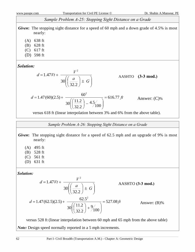
Sample Problem A-25: Stopping Sight Distance on a Grade
Given: The stopping sight distance for a speed of 60 mph and a down grade of 4.5% is most nearly:
(A) 638 ft (B) 628 ft (C) 617 ft (D) 598 ft
Solution:
±
+=Ga
VVtd
2.3230
47.12
AASHTO (3-3 mod.)
ftd 77.616
1005.4
2.322.1130
60)5.2)(60(47.12
=
−
+= Answer: (C)◄
versus 618 ft (linear interpolation between 3% and 6% from the above table).
Sample Problem A-26: Stopping Sight Distance on a Grade Given: The stopping sight distance for a speed of 62.5 mph and an upgrade of 9% is most
nearly:
(A) 495 ft (B) 528 ft (C) 561 ft (D) 631 ft
Solution:
±
+=Ga
VVtd
2.3230
47.12
AASHTO (3-3 mod.)
ftd 08.527
1009
2.322.1130
5.62)5.2)(5.62(47.12
=
+
+= Answer: (B)◄
versus 528 ft (linear interpolation between 60 mph and 65 mph from the above table)
Note: Design speed normally reported in a 5 mph increments.
www.passpe.com Transportation for Civil Engineering (PE) License © Dr. Shahin A. Mansour, PE
Part I- Civil Breadth (Transportation A.M.) - Chapter A: Geometric Design 63
A.3.1.3 Variations for Trucks:
The recommended stopping sight distances given in the previous table and the equations are based on passenger car operation and don not explicitly consider design for truck operation. Trucks as a whole, especially the larger and heavier units, need longer stopping distances for a given speed than passenger vehicles. However, there is one factor that tends to balance the additional barking lengths for trucks with those for passenger cars. The truck driver is able to see substantially farther beyond vertical sight obstructions because of the higher position of the seat in the vehicle.
www.passpe.com Transportation for Civil PE License © Dr. Shahin A.Mansour, PE
Part I- Civil Breadth (Transportation A.M.) - Chapter A: Geometric Design 64
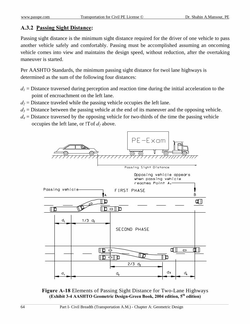
A.3.2 Passing Sight Distance: Passing sight distance is the minimum sight distance required for the driver of one vehicle to pass another vehicle safely and comfortably. Passing must be accomplished assuming an oncoming vehicle comes into view and maintains the design speed, without reduction, after the overtaking maneuver is started.
Per AASHTO Standards, the minimum passing sight distance for two–lane highways is determined as the sum of the following four distances:
d1 = Distance traversed during perception and reaction time during the initial acceleration to the point of encroachment on the left lane.
d2 = Distance traveled while the passing vehicle occupies the left lane. d3 = Distance between the passing vehicle at the end of its maneuver and the opposing vehicle. d4 = Distance traversed by the opposing vehicle for two-thirds of the time the passing vehicle
occupies the left lane, or ⅔ of d2 above.
Figure A-18 Elements of Passing Sight Distance for Two-Lane Highways (Exhibit 3-4 AASHTO Geometric Design-Green Book, 2004 edition, 5th edition)
www.passpe.com Transportation for Civil Engineering (PE) License © Dr. Shahin A. Mansour, PE
Part I- Civil Breadth (Transportation A.M.) - Chapter A: Geometric Design 65
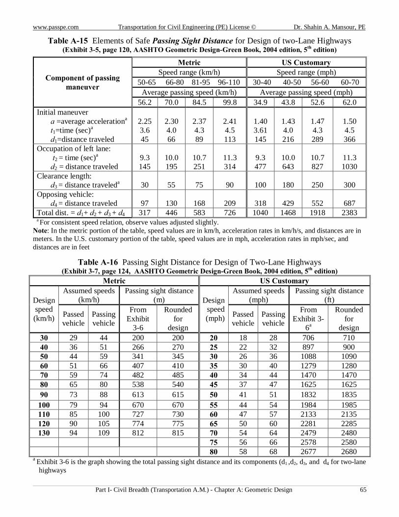
Table A-15 Elements of Safe Passing Sight Distance for Design of two-Lane Highways
(Exhibit 3-5, page 120, AASHTO Geometric Design-Green Book, 2004 edition, 5th edition)
Component of passing maneuver
Metric US Customary Speed range (km/h) Speed range (mph)
50-65 66-80 81-95 96-110 30-40 40-50 56-60 60-70 Average passing speed (km/h) Average passing speed (mph)
56.2 70.0 84.5 99.8 34.9 43.8 52.6 62.0 Initial maneuver a =average accelerationa t1=time (sec)a
d1=distance traveled
2.25 3.6 45
2.30 4.0 66
2.37 4.3 89
2.41 4.5 113
1.40 3.61 145
1.43 4.0 216
1.47 4.3 289
1.50 4.5 366
Occupation of left lane: t2 = time (sec)a d2 = distance traveled
9.3 145
10.0 195
10.7 251
11.3 314
9.3 477
10.0 643
10.7 827
11.3 1030
Clearance length: d3 = distance traveleda
30
55
75
90
100
180
250
300
Opposing vehicle: d4 = distance traveled
97
130
168
209
318
429
552
687
Total dist. = d1+ d2 + d3 + d4 317 446 583 726 1040 1468 1918 2383 a For consistent speed relation, observe values adjusted slightly. Note: In the metric portion of the table, speed values are in km/h, acceleration rates in km/h/s, and distances are in meters. In the U.S. customary portion of the table, speed values are in mph, acceleration rates in mph/sec, and distances are in feet
Table A-16 Passing Sight Distance for Design of Two-Lane Highways (Exhibit 3-7, page 124, AASHTO Geometric Design-Green Book, 2004 edition, 5th edition)
Metric US Customary
Design speed (km/h)
Assumed speeds (km/h)
Passing sight distance (m) Design
speed (mph)
Assumed speeds (mph)
Passing sight distance (ft)
Passed vehicle
Passing vehicle
From Exhibit
3-6
Rounded for
design
Passed vehicle
Passing vehicle
From Exhibit 3-
6a
Rounded for
design 30 29 44 200 200 20 18 28 706 710 40 36 51 266 270 25 22 32 897 900 50 44 59 341 345 30 26 36 1088 1090 60 51 66 407 410 35 30 40 1279 1280 70 59 74 482 485 40 34 44 1470 1470 80 65 80 538 540 45 37 47 1625 1625 90 73 88 613 615 50 41 51 1832 1835
100 79 94 670 670 55 44 54 1984 1985 110 85 100 727 730 60 47 57 2133 2135 120 90 105 774 775 65 50 60 2281 2285 130 94 109 812 815 70 54 64 2479 2480
75 56 66 2578 2580 80 58 68 2677 2680
a Exhibit 3-6 is the graph showing the total passing sight distance and its components (d1 ,d2, d3, and d4 for two-lane highways
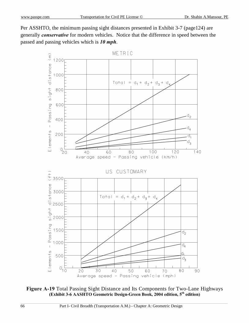
www.passpe.com Transportation for Civil PE License © Dr. Shahin A.Mansour, PE
Part I- Civil Breadth (Transportation A.M.) - Chapter A: Geometric Design 66
Per ASSHTO, the minimum passing sight distances presented in Exhibit 3-7 (page124) are generally conservative for modern vehicles. Notice that the difference in speed between the passed and passing vehicles which is 10 mph.
Figure A-19 Total Passing Sight Distance and Its Components for Two-Lane Highways (Exhibit 3-6 AASHTO Geometric Design-Green Book, 2004 edition, 5th edition)
www.passpe.com Transportation for Civil Engineering (PE) License © Dr. Shahin A. Mansour, PE
Part I- Civil Breadth (Transportation A.M.) - Chapter A: Geometric Design 67
Sample Problem A-27: Passing Sight Distance on a Grade
Given: The passing sight distance for a design speed of 55 mph assumed the passed vehicle is at 44 mph is most nearly:
(A) 1835 ft (B) 1985 ft (C) 2135 ft (D) 2285 ft
Solution:
Using AASHTO Exhibit 3-7 (Table A-19), the passing sight distance is 1985 ft.
Answer: (B)◄
A.3.3 Length of Crest Vertical Curves and Sight Distances:
Minimum lengths of crest vertical curves based on sight distance criteria generally are satisfactory from the standpoint of safety, comfort, and appearance.
Table A-17 Crest Vertical Curve Length and Sight Distances (Page 267- AASHTO Geometric Design-Green Book, 2004 edition, 5th edition)
Cre
st V
erti
cal C
urve
Len
gth
&
Sig
ht D
ista
nces
(S
SD
& P
SD
)
Metric US Customary Where S is less than L, (S < L)
( )2
21
2
22100 hh
SAL+
=
Where S is less than L, (S < L)
( )2
21
2
22100 hh
SAL+
= (3-41)
Where S is greater than L, (S > L)
Ahh
SL2
21 )(2002
+−=
Where S is greater than L, (S > L)
Ahh
SL2
21 )(2002
+−= (3-42)
where: L = length of vertical curve, m; S = sight distance, m; A = algebraic difference in grades, percent h1 = height of eye above roadway surface, m; h2 = height of object above roadway surface, m
where: L = length of vertical curve, ft; S = sight distance, ft; A = algebraic difference in grades, percent h1 = height of eye above roadway surface, ft; h2 = height of object above roadway surface, ft
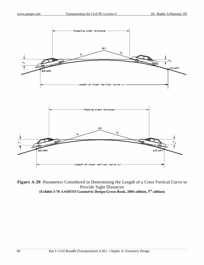
www.passpe.com Transportation for Civil PE License © Dr. Shahin A.Mansour, PE
Part I- Civil Breadth (Transportation A.M.) - Chapter A: Geometric Design 68
Figure A-20 Parameters Considered in Determining the Length of a Crest Vertical Curve to
Provide Sight Distances (Exhibit 3-70 AASHTO Geometric Design-Green Book, 2004 edition, 5th edition)
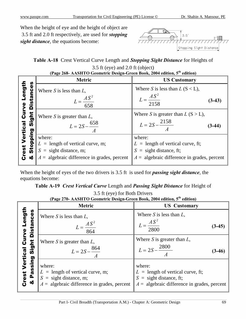
www.passpe.com Transportation for Civil Engineering (PE) License © Dr. Shahin A. Mansour, PE
Part I- Civil Breadth (Transportation A.M.) - Chapter A: Geometric Design 69
When the height of eye and the height of object are 3.5 ft and 2.0 ft respectively, are used for stopping sight distance, the equations become:
Table A-18 Crest Vertical Curve Length and Stopping Sight Distance for Heights of 3.5 ft (eye) and 2.0 ft (object)
(Page 268- AASHTO Geometric Design-Green Book, 2004 edition, 5th edition)
Cre
st V
erti
cal C
urve
Len
gth
& S
topp
ing
Sig
ht D
ista
nces
Metric US Customary Where S is less than L,
658
2SAL =
Where S is less than L (S < L),
2158
2SAL = (3-43)
Where S is greater than L,
ASL 6582 −=
Where S is greater than L (S > L),
ASL 21582 −= (3-44)
where: L = length of vertical curve, m; S = sight distance, m; A = algebraic difference in grades, percent
where: L = length of vertical curve, ft; S = sight distance, ft; A = algebraic difference in grades, percent
When the height of eyes of the two drivers is 3.5 ft is used for passing sight distance, the equations become:
Table A-19 Crest Vertical Curve Length and Passing Sight Distance for Height of 3.5 ft (eye) for Both Drivers
(Page 270- AASHTO Geometric Design-Green Book, 2004 edition, 5th edition)
Cre
st V
erti
cal C
urve
Len
gth
& P
assi
ng S
ight
Dis
tanc
es Metric US Customary
Where S is less than L,
864
2SAL =
Where S is less than L,
2800
2SAL = (3-45)
Where S is greater than L,
ASL 8642 −=
Where S is greater than L,
ASL 28002 −= (3-46)
where: L = length of vertical curve, m; S = sight distance, m; A = algebraic difference in grades, percent
where: L = length of vertical curve, ft; S = sight distance, ft; A = algebraic difference in grades, percent
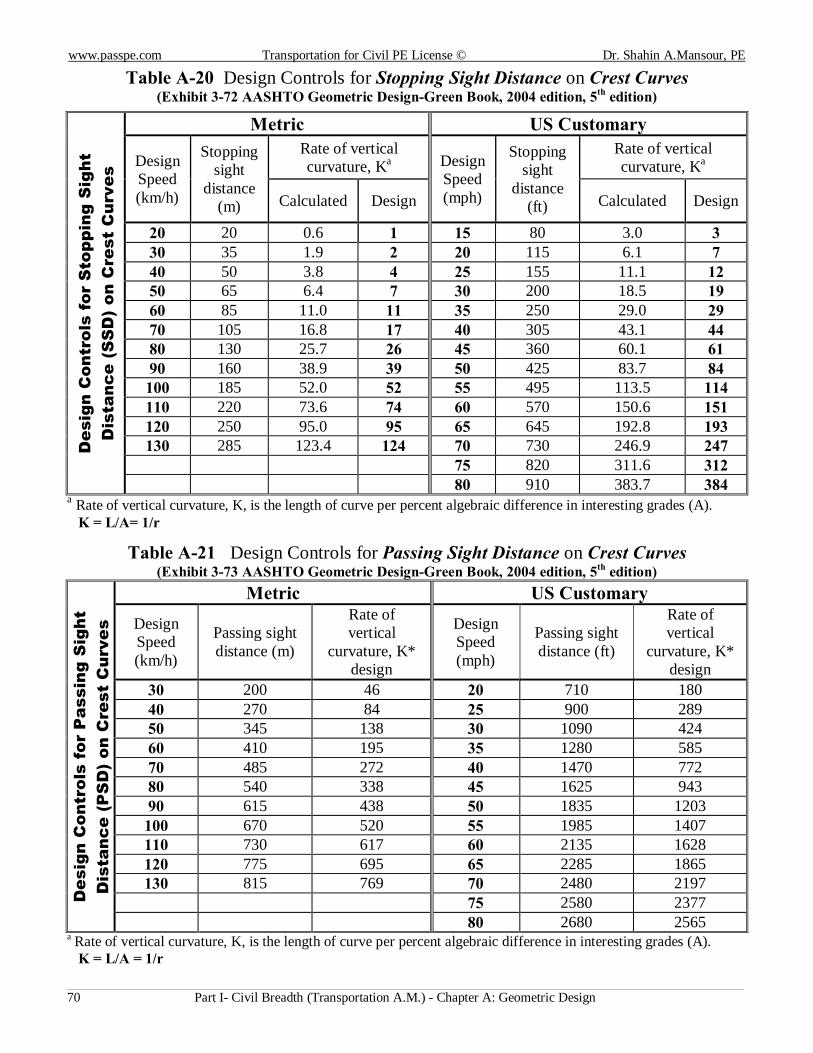
www.passpe.com Transportation for Civil PE License © Dr. Shahin A.Mansour, PE
Part I- Civil Breadth (Transportation A.M.) - Chapter A: Geometric Design 70
Table A-20 Design Controls for Stopping Sight Distance on Crest Curves (Exhibit 3-72 AASHTO Geometric Design-Green Book, 2004 edition, 5th edition)
Des
ign
Con
trol
s fo
r S
topp
ing
Sig
ht
Dis
tanc
e (S
SD
) on
Cre
st C
urve
s Metric US Customary
Design Speed (km/h)
Stopping sight
distance (m)
Rate of vertical curvature, Ka Design
Speed (mph)
Stopping sight
distance (ft)
Rate of vertical curvature, Ka
Calculated Design Calculated Design
20 20 0.6 1 15 80 3.0 3 30 35 1.9 2 20 115 6.1 7 40 50 3.8 4 25 155 11.1 12 50 65 6.4 7 30 200 18.5 19 60 85 11.0 11 35 250 29.0 29 70 105 16.8 17 40 305 43.1 44 80 130 25.7 26 45 360 60.1 61 90 160 38.9 39 50 425 83.7 84 100 185 52.0 52 55 495 113.5 114 110 220 73.6 74 60 570 150.6 151 120 250 95.0 95 65 645 192.8 193 130 285 123.4 124 70 730 246.9 247
75 820 311.6 312 80 910 383.7 384
a Rate of vertical curvature, K, is the length of curve per percent algebraic difference in interesting grades (A). K = L/A= 1/r
Table A-21 Design Controls for Passing Sight Distance on Crest Curves (Exhibit 3-73 AASHTO Geometric Design-Green Book, 2004 edition, 5th edition)
Des
ign
Con
trol
s fo
r P
assi
ng S
ight
D
ista
nce
(PS
D)
on C
rest
Cur
ves
Metric US Customary Design Speed (km/h)
Passing sight distance (m)
Rate of vertical
curvature, K* design
Design Speed (mph)
Passing sight distance (ft)
Rate of vertical
curvature, K* design
30 200 46 20 710 180 40 270 84 25 900 289 50 345 138 30 1090 424 60 410 195 35 1280 585 70 485 272 40 1470 772 80 540 338 45 1625 943 90 615 438 50 1835 1203 100 670 520 55 1985 1407 110 730 617 60 2135 1628 120 775 695 65 2285 1865 130 815 769 70 2480 2197
75 2580 2377 80 2680 2565
a Rate of vertical curvature, K, is the length of curve per percent algebraic difference in interesting grades (A). K = L/A = 1/r
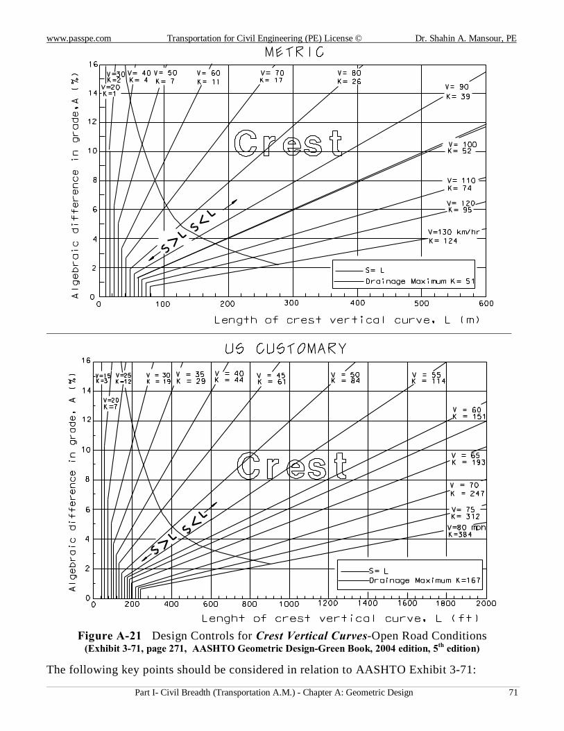
www.passpe.com Transportation for Civil Engineering (PE) License © Dr. Shahin A. Mansour, PE
Part I- Civil Breadth (Transportation A.M.) - Chapter A: Geometric Design 71
Figure A-21 Design Controls for Crest Vertical Curves-Open Road Conditions (Exhibit 3-71, page 271, AASHTO Geometric Design-Green Book, 2004 edition, 5th edition)
The following key points should be considered in relation to AASHTO Exhibit 3-71:
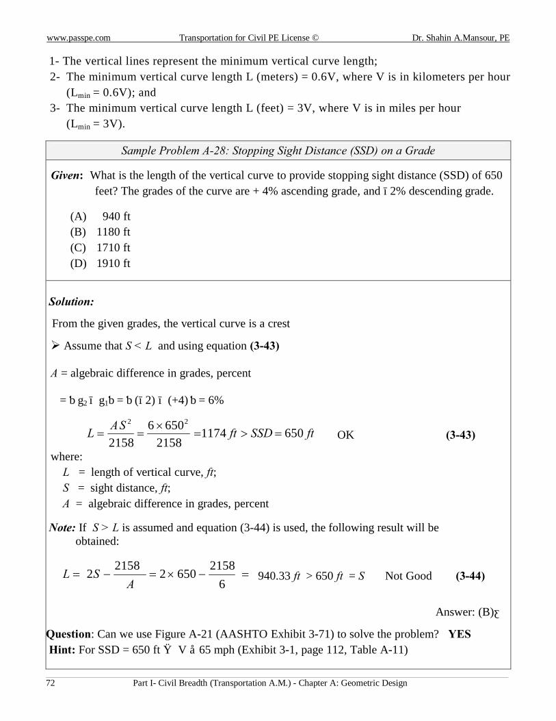
www.passpe.com Transportation for Civil PE License © Dr. Shahin A.Mansour, PE
Part I- Civil Breadth (Transportation A.M.) - Chapter A: Geometric Design 72
1- The vertical lines represent the minimum vertical curve length; 2- The minimum vertical curve length L (meters) = 0.6V, where V is in kilometers per hour
(Lmin = 0.6V); and
3- The minimum vertical curve length L (feet) = 3V, where V is in miles per hour
(Lmin = 3V).
Sample Problem A-28: Stopping Sight Distance (SSD) on a Grade
Given: What is the length of the vertical curve to provide stopping sight distance (SSD) of 650 feet? The grades of the curve are + 4% ascending grade, and −2% descending grade.
(A) 940 ft (B) 1180 ft (C) 1710 ft (D) 1910 ft
Solution:
From the given grades, the vertical curve is a crest
Ø Assume that S < L and using equation (3-43) A = algebraic difference in grades, percent = │g2 − g1│= │(−2) − (+4) │= 6%
ftSSDftSAL 65011742158
65062158
22
=>=×
== OK (3-43)
where: L = length of vertical curve, ft; S = sight distance, ft;
A = algebraic difference in grades, percent
Note: If S > L is assumed and equation (3-44) is used, the following result will be obtained:
=−×=−=6
21586502
21582
ASL 940.33 ft > 650 ft = S Not Good (3-44)
Answer: (B)◄
Question: Can we use Figure A-21 (AASHTO Exhibit 3-71) to solve the problem? YES Hint: For SSD = 650 ft → V ≈ 65 mph (Exhibit 3-1, page 112, Table A-11)
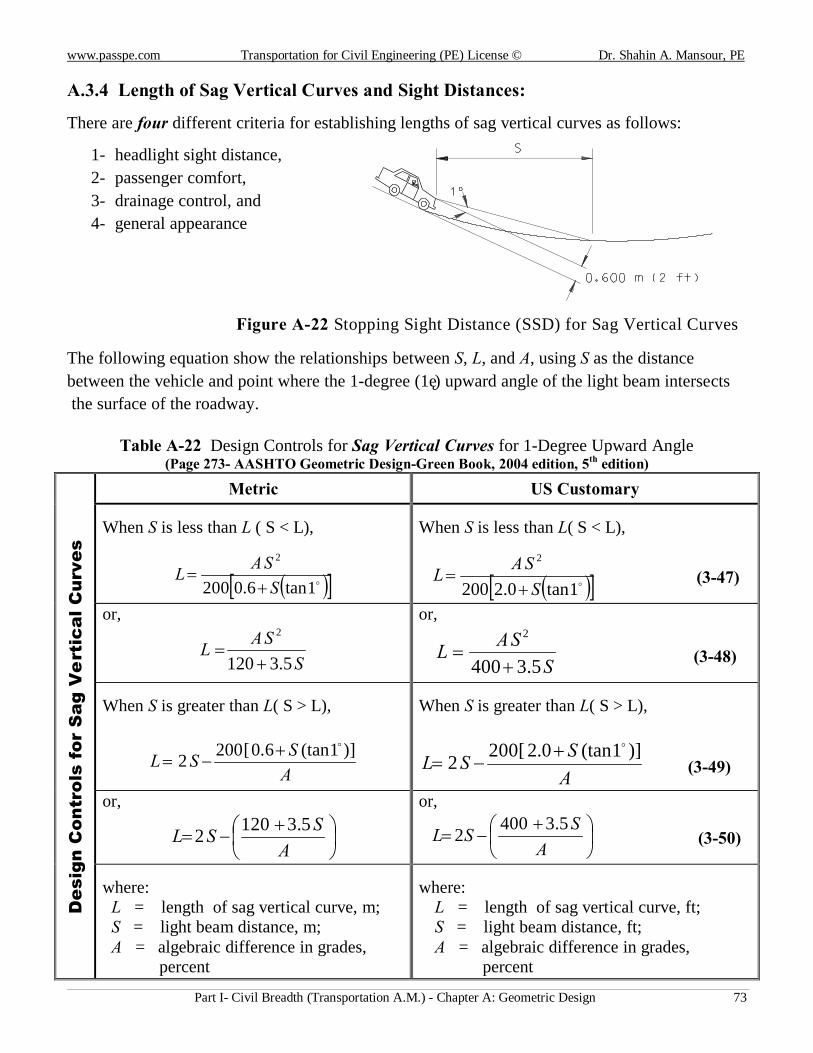
www.passpe.com Transportation for Civil Engineering (PE) License © Dr. Shahin A. Mansour, PE
Part I- Civil Breadth (Transportation A.M.) - Chapter A: Geometric Design 73
A.3.4 Length of Sag Vertical Curves and Sight Distances:
There are four different criteria for establishing lengths of sag vertical curves as follows:
1- headlight sight distance, 2- passenger comfort, 3- drainage control, and 4- general appearance
Figure A-22 Stopping Sight Distance (SSD) for Sag Vertical Curves
The following equation show the relationships between S, L, and A, using S as the distance between the vehicle and point where the 1-degree (1˚) upward angle of the light beam intersects the surface of the roadway.
Table A-22 Design Controls for Sag Vertical Curves for 1-Degree Upward Angle (Page 273- AASHTO Geometric Design-Green Book, 2004 edition, 5th edition)
Des
ign
Con
trol
s fo
r S
ag V
ert
ical
Cur
ves
Metric US Customary
When S is less than L ( S < L),
( )[ ]o1tan6.0200
2
SSAL
+=
When S is less than L( S < L),
( )[ ]o1tan0.2200
2
SSAL
+= (3-47)
or,
SSAL
5.3120
2
+=
or,
SSAL
5.3400
2
+= (3-48)
When S is greater than L( S > L),
ASSL )]1(tan6.0[2002
o+−=
When S is greater than L( S > L),
ASSL )]1(tan0.2[2002
o+−= (3-49)
or,
+
−=A
SSL 5.31202
or,
+
−=A
SSL 5.34002 (3-50)
where: L = length of sag vertical curve, m; S = light beam distance, m; A = algebraic difference in grades, percent
where: L = length of sag vertical curve, ft; S = light beam distance, ft; A = algebraic difference in grades, percent
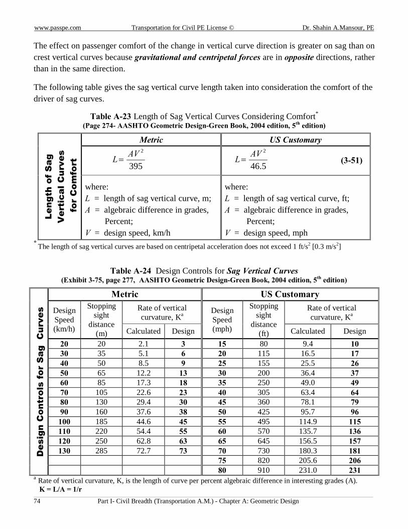
www.passpe.com Transportation for Civil PE License © Dr. Shahin A.Mansour, PE
Part I- Civil Breadth (Transportation A.M.) - Chapter A: Geometric Design 74
The effect on passenger comfort of the change in vertical curve direction is greater on sag than on crest vertical curves because gravitational and centripetal forces are in opposite directions, rather than in the same direction.
The following table gives the sag vertical curve length taken into consideration the comfort of the driver of sag curves.
Table A-23 Length of Sag Vertical Curves Considering Comfort* (Page 274- AASHTO Geometric Design-Green Book, 2004 edition, 5th edition)
Leng
th o
f S
ag
Ver
tica
l Cur
ves
for
Com
fort
Metric US Customary
395
2AVL = 5.46
2AVL = (3-51)
where: L = length of sag vertical curve, m; A = algebraic difference in grades, Percent; V = design speed, km/h
where: L = length of sag vertical curve, ft; A = algebraic difference in grades, Percent; V = design speed, mph
* The length of sag vertical curves are based on centripetal acceleration does not exceed 1 ft/s2 [0.3 m/s2]
Table A-24 Design Controls for Sag Vertical Curves (Exhibit 3-75, page 277, AASHTO Geometric Design-Green Book, 2004 edition, 5th edition)
Des
ign
Con
trol
s fo
r S
ag C
urve
s
Metric US Customary
Design Speed (km/h)
Stopping sight
distance (m)
Rate of vertical curvature, Ka
Design Speed (mph)
Stopping sight
distance (ft)
Rate of vertical curvature, Ka
Calculated Design Calculated Design 20 20 2.1 3 15 80 9.4 10 30 35 5.1 6 20 115 16.5 17 40 50 8.5 9 25 155 25.5 26 50 65 12.2 13 30 200 36.4 37 60 85 17.3 18 35 250 49.0 49 70 105 22.6 23 40 305 63.4 64 80 130 29.4 30 45 360 78.1 79 90 160 37.6 38 50 425 95.7 96 100 185 44.6 45 55 495 114.9 115 110 220 54.4 55 60 570 135.7 136 120 250 62.8 63 65 645 156.5 157 130 285 72.7 73 70 730 180.3 181
75 820 205.6 206 80 910 231.0 231
a Rate of vertical curvature, K, is the length of curve per percent algebraic difference in interesting grades (A). K = L/A = 1/r
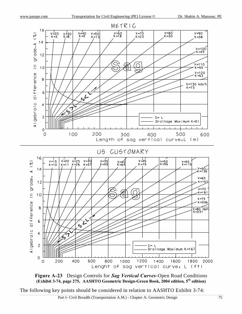
www.passpe.com Transportation for Civil Engineering (PE) License © Dr. Shahin A. Mansour, PE
Part I- Civil Breadth (Transportation A.M.) - Chapter A: Geometric Design 75
Figure A-23 Design Controls for Sag Vertical Curves-Open Road Conditions (Exhibit 3-74, page 275, AASHTO Geometric Design-Green Book, 2004 edition, 5th edition)
The following key points should be considered in relation to AASHTO Exhibit 3-74:
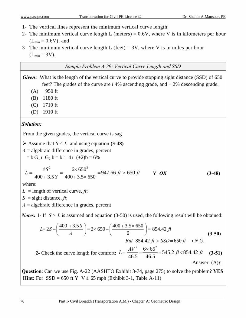
www.passpe.com Transportation for Civil PE License © Dr. Shahin A.Mansour, PE
Part I- Civil Breadth (Transportation A.M.) - Chapter A: Geometric Design 76
1- The vertical lines represent the minimum vertical curve length; 2- The minimum vertical curve length L (meters) = 0.6V, where V is in kilometers per hour
(Lmin = 0.6V); and 3- The minimum vertical curve length L (feet) = 3V, where V is in miles per hour
(Lmin = 3V).
Sample Problem A-29: Vertical Curve Length and SSD
Given: What is the length of the vertical curve to provide stopping sight distance (SSD) of 650 feet? The grades of the curve are −4% ascending grade, and + 2% descending grade.
(A) 950 ft (B) 1180 ft (C) 1710 ft (D) 1910 ft
Solution:
From the given grades, the vertical curve is sag
Ø Assume that S < L and using equation (3-48) A = algebraic difference in grades, percent = │G1 − G2 │= │ − 4 − (+2)│= 6%
ftftS
SAL 65066.9476505.3400
65065.3400
22
>=×+
×=+
= → OK (3-48)
where: L = length of vertical curve, ft; S = sight distance, ft; A = algebraic difference in grades, percent
Notes: 1- If S > L is assumed and equation (3-50) is used, the following result will be obtained:
..65042.854
42.8546
6505.340065025.34002
GNftSSDftBut
ftA
SSL
→=>
=
×+
−×=
+
−= (3-50)
2- Check the curve length for comfort: ftftAVL 42.8542.5455.46
6565.46
22
<=×
== (3-51)
Answer: (A)◄
Question: Can we use Fig. A-22 (AASHTO Exhibit 3-74, page 275) to solve the problem? YES Hint: For SSD = 650 ft → V ≈ 65 mph (Exhibit 3-1, Table A-11)
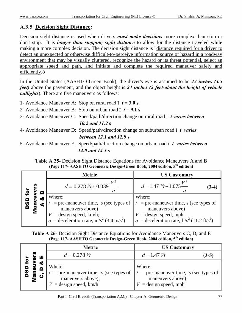
www.passpe.com Transportation for Civil Engineering (PE) License © Dr. Shahin A. Mansour, PE
Part I- Civil Breadth (Transportation A.M.) - Chapter A: Geometric Design 77
A.3.5 Decision Sight Distance:
Decision sight distance is used when drivers must make decisions more complex than stop or don't stop. It is longer than stopping sight distance to allow for the distance traveled while making a more complex decision. The decision sight distance is "distance required for a driver to detect an unexpected or otherwise difficult-to-perceive information source or hazard in a roadway environment that may be visually cluttered, recognize the hazard or its threat potential, select an appropriate speed and path, and initiate and complete the required maneuver safely and efficiently.”
In the United States (AASHTO Green Book), the driver's eye is assumed to be 42 inches (3.5 feet) above the pavement, and the object height is 24 inches (2 feet-about the height of vehicle taillights). There are five maneuvers as follows:
1- Avoidance Maneuver A: Stop on rural road − t = 3.0 s 2- Avoidance Maneuver B: Stop on urban road − t = 9.1 s 3- Avoidance Maneuver C: Speed/path/direction change on rural road − t varies between 10.2 and 11.2 s 4- Avoidance Maneuver D: Speed/path/direction change on suburban road − t varies between 12.1 and 12.9 s 5- Avoidance Maneuver E: Speed/path/direction change on urban road − t varies between 14.0 and 14.5 s
Table A 25- Decision Sight Distance Equations for Avoidance Maneuvers A and B (Page 117- AASHTO Geometric Design-Green Book, 2004 edition, 5th edition)
DS
D f
or
Man
euve
rs
A &
B
Metric US Customary
aVVtd
2
039.0278.0 += a
VVtd2
075.147.1 += (3-4)
Where: t = pre-maneuver time, s (see types of
maneuvers above) V = design speed, km/h; a = deceleration rate, m/s2 (3.4 m/s2)
Where: t = pre-maneuver time, s (see types of
maneuvers above) V = design speed, mph; a = deceleration rate, ft/s2 (11.2 ft/s2)
Table A 26- Decision Sight Distance Equations for Avoidance Maneuvers C, D, and E (Page 117- AASHTO Geometric Design-Green Book, 2004 edition, 5th edition)
DS
D f
or
Man
euve
rs
C, D
& E
Metric US Customary Vtd 278.0= Vtd 47.1= (3-5)
Where: t = pre-maneuver time, s (see types of
maneuvers above); V = design speed, km/h
Where: t = pre-maneuver time, s (see types of
maneuvers above); V = design speed, mph
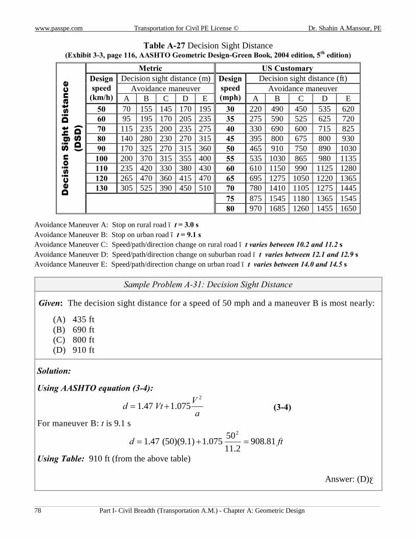
www.passpe.com Transportation for Civil PE License © Dr. Shahin A.Mansour, PE
Part I- Civil Breadth (Transportation A.M.) - Chapter A: Geometric Design 78
Table A-27 Decision Sight Distance (Exhibit 3-3, page 116, AASHTO Geometric Design-Green Book, 2004 edition, 5th edition)
D
ecis
ion
Sig
ht D
ista
nce
(DS
D)
Metric US Customary Design speed
(km/h)
Decision sight distance (m) Design speed (mph)
Decision sight distance (ft) Avoidance maneuver Avoidance maneuver
A B C D E A B C D E 50 70 155 145 170 195 30 220 490 450 535 620 60 95 195 170 205 235 35 275 590 525 625 720 70 115 235 200 235 275 40 330 690 600 715 825 80 140 280 230 270 315 45 395 800 675 800 930 90 170 325 270 315 360 50 465 910 750 890 1030 100 200 370 315 355 400 55 535 1030 865 980 1135 110 235 420 330 380 430 60 610 1150 990 1125 1280 120 265 470 360 415 470 65 695 1275 1050 1220 1365 130 305 525 390 450 510 70 780 1410 1105 1275 1445
75 875 1545 1180 1365 1545 80 970 1685 1260 1455 1650
Avoidance Maneuver A: Stop on rural road − t = 3.0 s Avoidance Maneuver B: Stop on urban road − t = 9.1 s Avoidance Maneuver C: Speed/path/direction change on rural road − t varies between 10.2 and 11.2 s Avoidance Maneuver D: Speed/path/direction change on suburban road − t varies between 12.1 and 12.9 s Avoidance Maneuver E: Speed/path/direction change on urban road − t varies between 14.0 and 14.5 s
Sample Problem A-31: Decision Sight Distance
Given: The decision sight distance for a speed of 50 mph and a maneuver B is most nearly:
(A) 435 ft (B) 690 ft (C) 800 ft (D) 910 ft
Solution: Using AASHTO equation (3-4):
aVVtd
2
075.147.1 += (3-4)
For maneuver B: t is 9.1 s
ftd 81.9082.11
50075.1)1.9)(50(47.12
=+=
Using Table: 910 ft (from the above table)
Answer: (D)◄
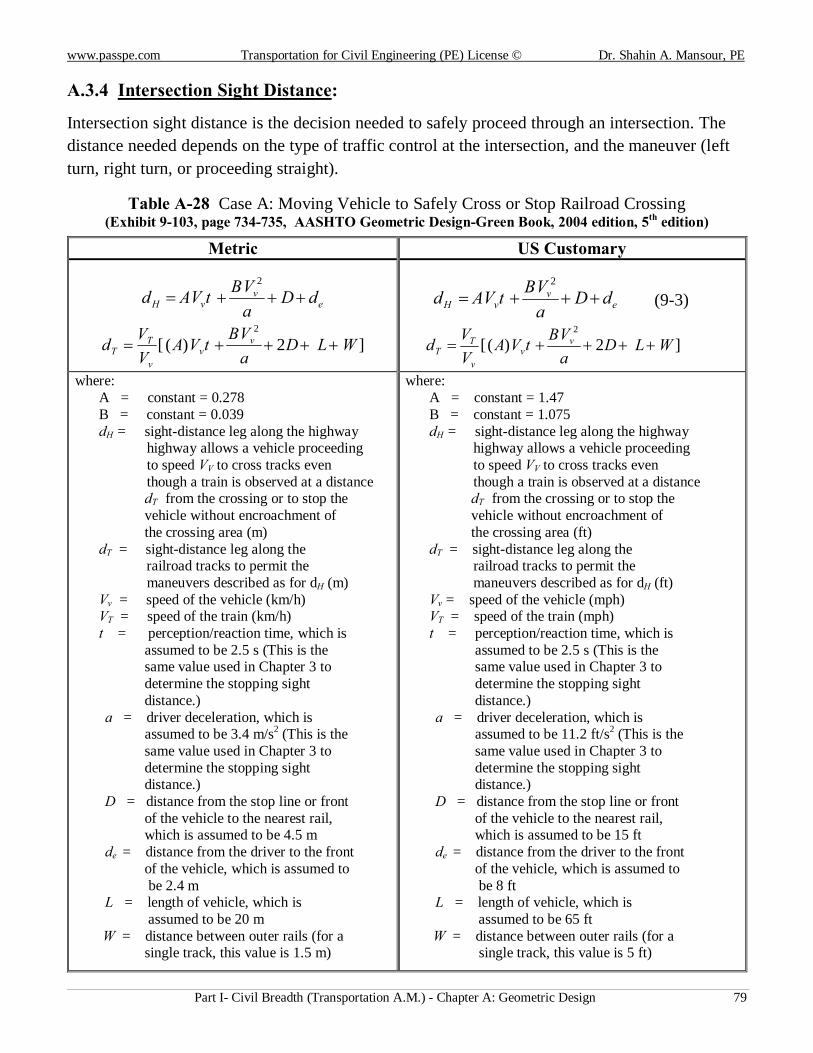
www.passpe.com Transportation for Civil Engineering (PE) License © Dr. Shahin A. Mansour, PE
Part I- Civil Breadth (Transportation A.M.) - Chapter A: Geometric Design 79
A.3.4 Intersection Sight Distance:
Intersection sight distance is the decision needed to safely proceed through an intersection. The distance needed depends on the type of traffic control at the intersection, and the maneuver (left turn, right turn, or proceeding straight).
Table A-28 Case A: Moving Vehicle to Safely Cross or Stop Railroad Crossing (Exhibit 9-103, page 734-735, AASHTO Geometric Design-Green Book, 2004 edition, 5th edition)
Metric US Customary
ev
vH dDaVBtAVd +++=
2
]2)([2
WLDaVBtVA
VVd v
vv
TT ++++=
ev
vH dDaVBtAVd +++=
2
(9-3)
]2)([2
WLDaVBtVA
VVd v
vv
TT ++++=
where: A = constant = 0.278 B = constant = 0.039 dH = sight-distance leg along the highway highway allows a vehicle proceeding to speed VV to cross tracks even though a train is observed at a distance
dT from the crossing or to stop the vehicle without encroachment of the crossing area (m)
dT = sight-distance leg along the railroad tracks to permit the maneuvers described as for dH (m) Vv = speed of the vehicle (km/h) VT = speed of the train (km/h) t = perception/reaction time, which is
assumed to be 2.5 s (This is the same value used in Chapter 3 to determine the stopping sight distance.)
a = driver deceleration, which is assumed to be 3.4 m/s2 (This is the same value used in Chapter 3 to determine the stopping sight distance.)
D = distance from the stop line or front of the vehicle to the nearest rail, which is assumed to be 4.5 m
de = distance from the driver to the front of the vehicle, which is assumed to be 2.4 m
L = length of vehicle, which is assumed to be 20 m
W = distance between outer rails (for a single track, this value is 1.5 m)
where: A = constant = 1.47 B = constant = 1.075 dH = sight-distance leg along the highway highway allows a vehicle proceeding to speed VV to cross tracks even though a train is observed at a distance
dT from the crossing or to stop the vehicle without encroachment of the crossing area (ft)
dT = sight-distance leg along the railroad tracks to permit the maneuvers described as for dH (ft) Vv = speed of the vehicle (mph) VT = speed of the train (mph) t = perception/reaction time, which is
assumed to be 2.5 s (This is the same value used in Chapter 3 to determine the stopping sight distance.)
a = driver deceleration, which is assumed to be 11.2 ft/s2 (This is the same value used in Chapter 3 to determine the stopping sight distance.)
D = distance from the stop line or front of the vehicle to the nearest rail, which is assumed to be 15 ft
de = distance from the driver to the front of the vehicle, which is assumed to be 8 ft
L = length of vehicle, which is assumed to be 65 ft
W = distance between outer rails (for a single track, this value is 5 ft)
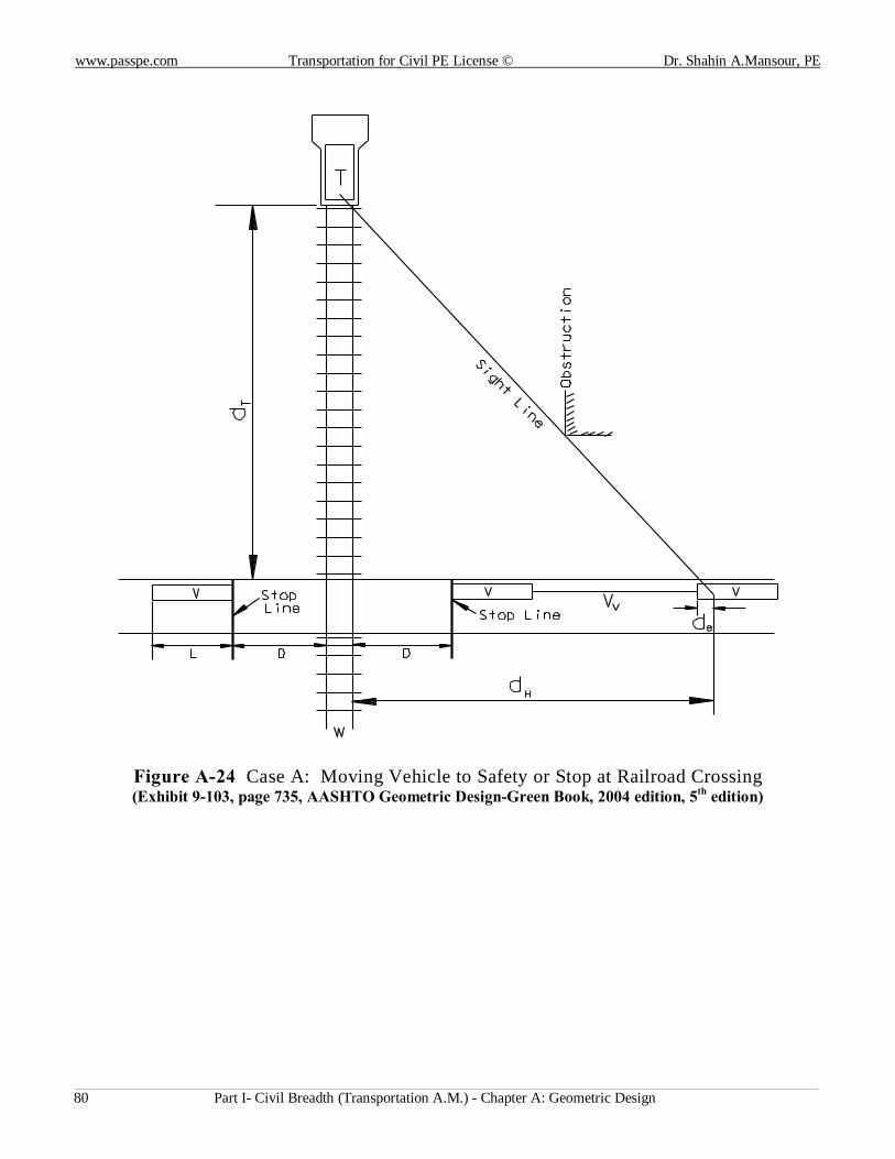
www.passpe.com Transportation for Civil PE License © Dr. Shahin A.Mansour, PE
Part I- Civil Breadth (Transportation A.M.) - Chapter A: Geometric Design 80
Figure A-24 Case A: Moving Vehicle to Safety or Stop at Railroad Crossing (Exhibit 9-103, page 735, AASHTO Geometric Design-Green Book, 2004 edition, 5th edition)
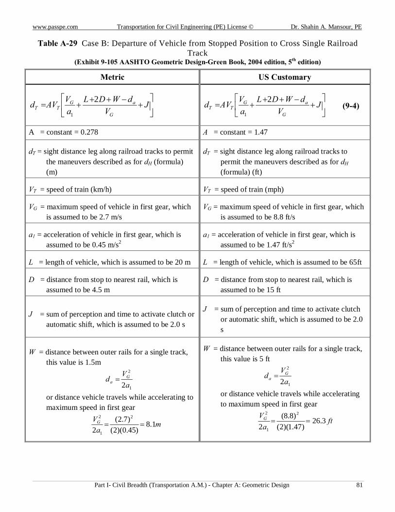
www.passpe.com Transportation for Civil Engineering (PE) License © Dr. Shahin A. Mansour, PE
Part I- Civil Breadth (Transportation A.M.) - Chapter A: Geometric Design 81
Table A-29 Case B: Departure of Vehicle from Stopped Position to Cross Single Railroad Track
(Exhibit 9-105 AASHTO Geometric Design-Green Book, 2004 edition, 5th edition)
Metric US Customary
+
−+++= J
VdWDL
aVVAd
G
aGTT
2
1
+
−+++= J
VdWDL
aVVAd
G
aGTT
2
1 (9-4)
A = constant = 0.278 A = constant = 1.47
dT = sight distance leg along railroad tracks to permit the maneuvers described as for dH (formula) (m)
dT = sight distance leg along railroad tracks to permit the maneuvers described as for dH (formula) (ft)
VT = speed of train (km/h)
VT = speed of train (mph)
VG = maximum speed of vehicle in first gear, which is assumed to be 2.7 m/s
VG = maximum speed of vehicle in first gear, which is assumed to be 8.8 ft/s
a1 = acceleration of vehicle in first gear, which is assumed to be 0.45 m/s2
a1 = acceleration of vehicle in first gear, which is assumed to be 1.47 ft/s2
L = length of vehicle, which is assumed to be 20 m
L = length of vehicle, which is assumed to be 65ft
D = distance from stop to nearest rail, which is assumed to be 4.5 m
D = distance from stop to nearest rail, which is assumed to be 15 ft
J = sum of perception and time to activate clutch or automatic shift, which is assumed to be 2.0 s
J = sum of perception and time to activate clutch or automatic shift, which is assumed to be 2.0 s
W = distance between outer rails for a single track, this value is 1.5m
1
2
2aV
d Ga =
or distance vehicle travels while accelerating to maximum speed in first gear
ma
VG 1.8)45.0)(2(
)7.2(2
2
1
2
==
W = distance between outer rails for a single track, this value is 5 ft
1
2
2aV
d Ga =
or distance vehicle travels while accelerating to maximum speed in first gear
fta
VG 3.26)47.1)(2(
)8.8(2
2
1
2
==
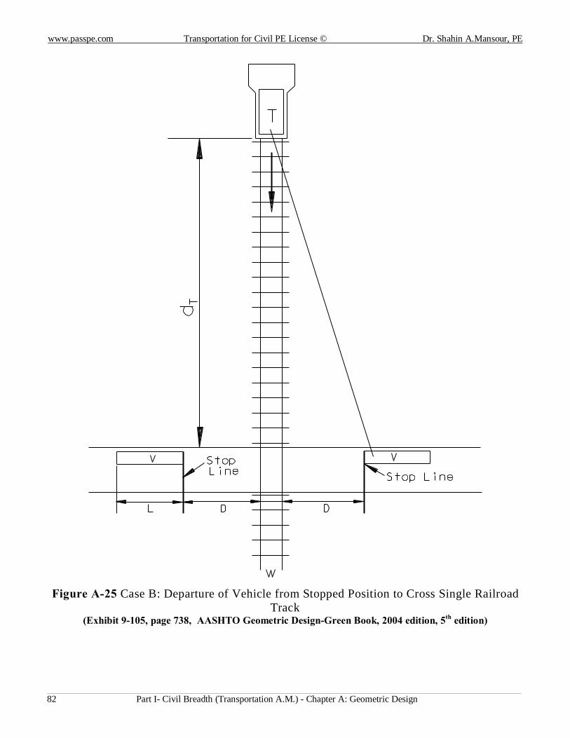
www.passpe.com Transportation for Civil PE License © Dr. Shahin A.Mansour, PE
Part I- Civil Breadth (Transportation A.M.) - Chapter A: Geometric Design 82
Figure A-25 Case B: Departure of Vehicle from Stopped Position to Cross Single Railroad Track
(Exhibit 9-105, page 738, AASHTO Geometric Design-Green Book, 2004 edition, 5th edition)
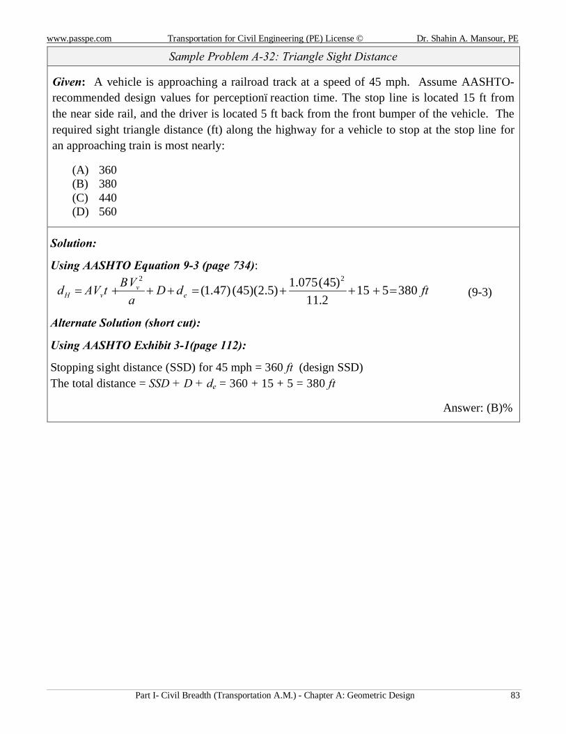
www.passpe.com Transportation for Civil Engineering (PE) License © Dr. Shahin A. Mansour, PE
Part I- Civil Breadth (Transportation A.M.) - Chapter A: Geometric Design 83
Sample Problem A-32: Triangle Sight Distance
Given: A vehicle is approaching a railroad track at a speed of 45 mph. Assume AASHTO- recommended design values for perception–reaction time. The stop line is located 15 ft from the near side rail, and the driver is located 5 ft back from the front bumper of the vehicle. The required sight triangle distance (ft) along the highway for a vehicle to stop at the stop line for an approaching train is most nearly:
(A) 360 (B) 380 (C) 440 (D) 560
Solution:
Using AASHTO Equation 9-3 (page 734):
ftdDaVBtAVd e
vvH 380515
2.11)45(075.1)5.2)(45()47.1(
22
=+++=+++= (9-3)
Alternate Solution (short cut):
Using AASHTO Exhibit 3-1(page 112):
Stopping sight distance (SSD) for 45 mph = 360 ft (design SSD) The total distance = SSD + D + de = 360 + 15 + 5 = 380 ft
Answer: (B)◄
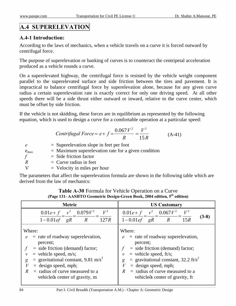
www.passpe.com Transportation for Civil PE License © Dr. Shahin A.Mansour, PE
Part I- Civil Breadth (Transportation A.M.) - Chapter A: Geometric Design 84
A.4 SUPERELEVATION
A.4-1 Introduction: According to the laws of mechanics, when a vehicle travels on a curve it is forced outward by centrifugal force.
The purpose of superelevation or banking of curves is to counteract the centripetal acceleration produced as a vehicle rounds a curve.
On a superelevated highway, the centrifugal force is resisted by the vehicle weight component parallel to the superelevated surface and side friction between the tires and pavement. It is impractical to balance centrifugal force by superelevation alone, because for any given curve radius a certain superelevation rate is exactly correct for only one driving speed. At all other speeds there will be a side thrust either outward or inward, relative to the curve center, which must be offset by side friction.
If the vehicle is not skidding, these forces are in equilibrium as represented by the following equation, which is used to design a curve for a comfortable operation at a particular speed:
RV
RVfeForcelCentrifuga
15067.0 22
==+= (A-41)
e = Superelevation slope in feet per foot emax = Maximum superelevation rate for a given condition f = Side friction factor R = Curve radius in feet V = Velocity in miles per hour
The parameters that affect the superelevation formula are shown in the following table which are derived from the law of mechanics:
Table A-30 Formula for Vehicle Operation on a Curve (Page 131- AASHTO Geometric Design-Green Book, 2004 edition, 5th edition)
Metric US Customary
RV
RV
gRv
effe
127079.0
01.0101.0 222
===−
+ R
VR
VgRv
effe
15067.0
01.0101.0 222
===−
+ (3-8)
Where: e = rate of roadway superelevation, percent; f = side friction (demand) factor; v = vehicle speed, m/s; g = gravitational constant, 9.81 m/s2 V = design speed, mph; R = radius of curve measured to a vehicle’s center of gravity, m
Where: e = rate of roadway superelevation, percent; f = side friction (demand) factor; v = vehicle speed, ft/s; g = gravitational constant, 32.2 ft/s2 V = design speed, mph; R = radius of curve measured to a vehicle’s center of gravity, ft
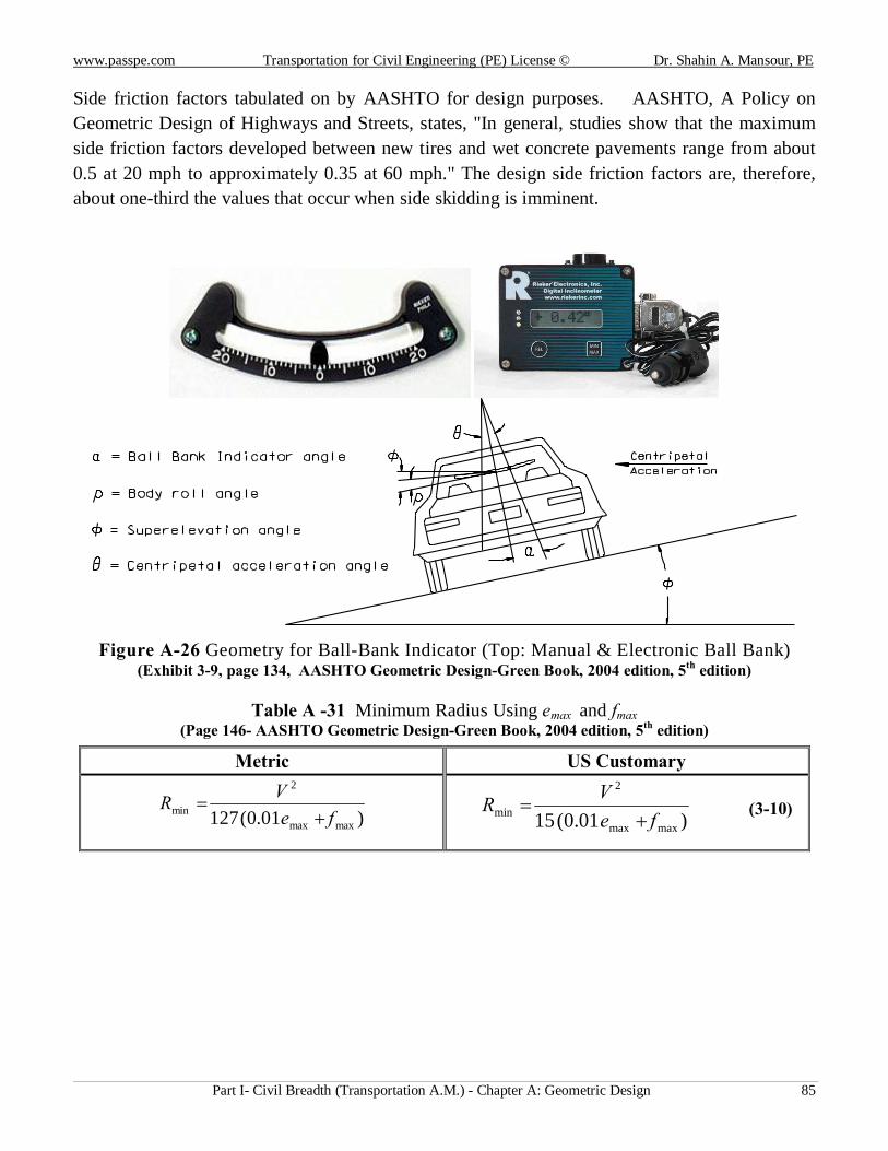
www.passpe.com Transportation for Civil Engineering (PE) License © Dr. Shahin A. Mansour, PE
Part I- Civil Breadth (Transportation A.M.) - Chapter A: Geometric Design 85
Side friction factors tabulated on by AASHTO for design purposes. AASHTO, A Policy on Geometric Design of Highways and Streets, states, "In general, studies show that the maximum side friction factors developed between new tires and wet concrete pavements range from about 0.5 at 20 mph to approximately 0.35 at 60 mph." The design side friction factors are, therefore, about one-third the values that occur when side skidding is imminent.
Figure A-26 Geometry for Ball-Bank Indicator (Top: Manual & Electronic Ball Bank) (Exhibit 3-9, page 134, AASHTO Geometric Design-Green Book, 2004 edition, 5th edition)
Table A -31 Minimum Radius Using emax and fmax (Page 146- AASHTO Geometric Design-Green Book, 2004 edition, 5th edition)
Metric US Customary
)01.0(127 maxmax
2
min feVR
+= )01.0(15 maxmax
2
min feVR
+= (3-10)
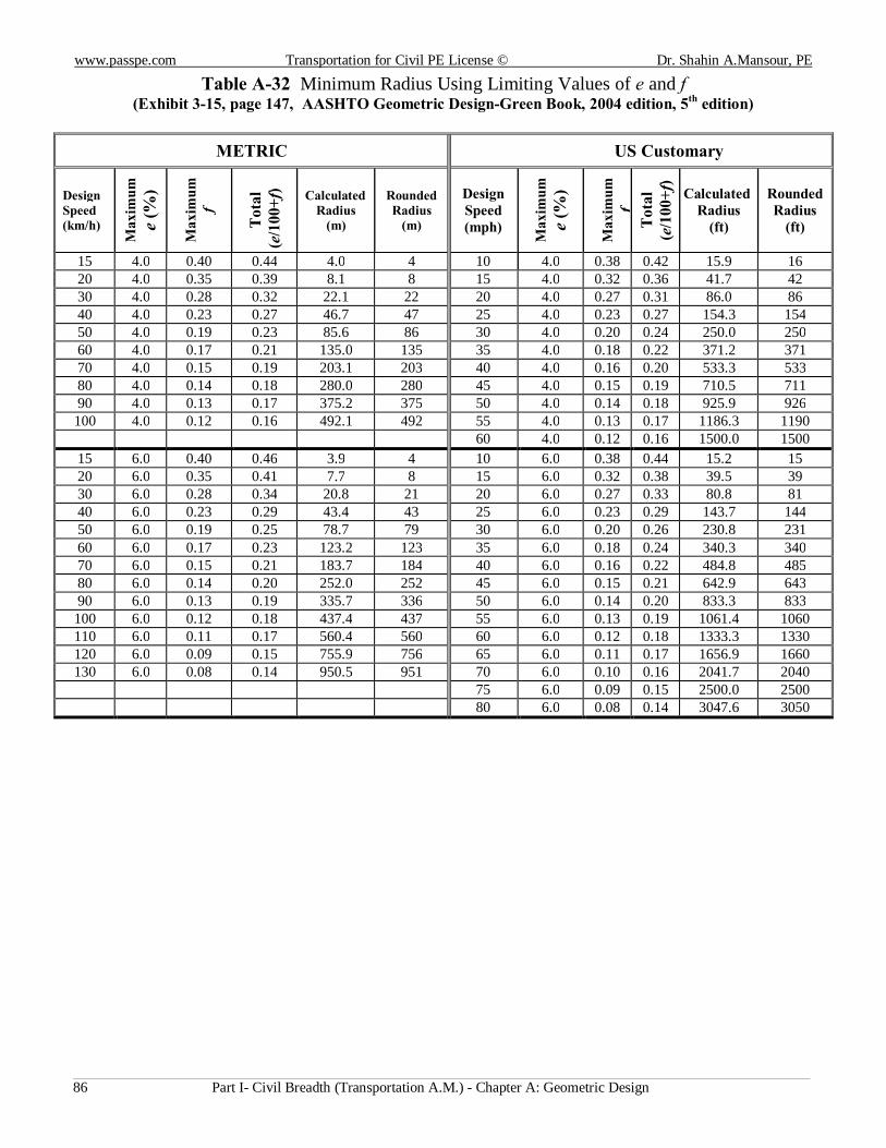
www.passpe.com Transportation for Civil PE License © Dr. Shahin A.Mansour, PE
Part I- Civil Breadth (Transportation A.M.) - Chapter A: Geometric Design 86
Table A-32 Minimum Radius Using Limiting Values of e and f (Exhibit 3-15, page 147, AASHTO Geometric Design-Green Book, 2004 edition, 5th edition)
METRIC US Customary
Design Speed (km/h)
Max
imum
e
(%)
Max
imum
f
Tot
al
(e/1
00+f
) Calculated
Radius (m)
Rounded Radius
(m)
Design Speed (mph)
Max
imum
e
(%)
M
axim
um
f T
otal
(e
/100
+f)
Calculated Radius
(ft)
Rounded Radius
(ft)
15 4.0 0.40 0.44 4.0 4 10 4.0 0.38 0.42 15.9 16 20 4.0 0.35 0.39 8.1 8 15 4.0 0.32 0.36 41.7 42 30 4.0 0.28 0.32 22.1 22 20 4.0 0.27 0.31 86.0 86 40 4.0 0.23 0.27 46.7 47 25 4.0 0.23 0.27 154.3 154 50 4.0 0.19 0.23 85.6 86 30 4.0 0.20 0.24 250.0 250 60 4.0 0.17 0.21 135.0 135 35 4.0 0.18 0.22 371.2 371 70 4.0 0.15 0.19 203.1 203 40 4.0 0.16 0.20 533.3 533 80 4.0 0.14 0.18 280.0 280 45 4.0 0.15 0.19 710.5 711 90 4.0 0.13 0.17 375.2 375 50 4.0 0.14 0.18 925.9 926 100 4.0 0.12 0.16 492.1 492 55 4.0 0.13 0.17 1186.3 1190
60 4.0 0.12 0.16 1500.0 1500 15 6.0 0.40 0.46 3.9 4 10 6.0 0.38 0.44 15.2 15 20 6.0 0.35 0.41 7.7 8 15 6.0 0.32 0.38 39.5 39 30 6.0 0.28 0.34 20.8 21 20 6.0 0.27 0.33 80.8 81 40 6.0 0.23 0.29 43.4 43 25 6.0 0.23 0.29 143.7 144 50 6.0 0.19 0.25 78.7 79 30 6.0 0.20 0.26 230.8 231 60 6.0 0.17 0.23 123.2 123 35 6.0 0.18 0.24 340.3 340 70 6.0 0.15 0.21 183.7 184 40 6.0 0.16 0.22 484.8 485 80 6.0 0.14 0.20 252.0 252 45 6.0 0.15 0.21 642.9 643 90 6.0 0.13 0.19 335.7 336 50 6.0 0.14 0.20 833.3 833 100 6.0 0.12 0.18 437.4 437 55 6.0 0.13 0.19 1061.4 1060 110 6.0 0.11 0.17 560.4 560 60 6.0 0.12 0.18 1333.3 1330 120 6.0 0.09 0.15 755.9 756 65 6.0 0.11 0.17 1656.9 1660 130 6.0 0.08 0.14 950.5 951 70 6.0 0.10 0.16 2041.7 2040
75 6.0 0.09 0.15 2500.0 2500 80 6.0 0.08 0.14 3047.6 3050
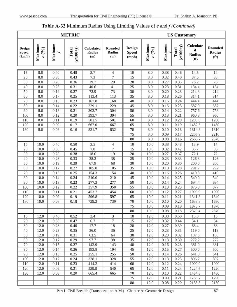
www.passpe.com Transportation for Civil Engineering (PE) License © Dr. Shahin A. Mansour, PE
Part I- Civil Breadth (Transportation A.M.) - Chapter A: Geometric Design 87
Table A-32 Minimum Radius Using Limiting Values of e and f (Continued)
METRIC US Customary
Design Speed (km/h)
Max
imum
e
(%)
Max
imum
f
Tot
al
(e/1
00+f
) Calculated
Radius (m)
Rounded Radius
(m)
Design Speed (mph)
Max
imum
e
(%)
M
axim
um
f T
otal
(e
/100
+f)
Calculate
d Radius
(ft)
Rounded Radius
(ft)
15 8.0 0.40 0.48 3.7 4 10 8.0 0.38 0.46 14.5 14 20 8.0 0.35 0.43 7.3 7 15 8.0 0.32 0.40 37.5 38 30 8.0 0.28 0.36 19.7 20 20 8.0 0.27 0.35 76.2 76 40 8.0 0.23 0.31 40.6 41 25 8.0 0.23 0.31 134.4 134 50 8.0 0.19 0.27 72.9 73 30 8.0 0.20 0.28 214.3 214 60 8.0 0.17 0.25 113.4 113 35 8.0 0.18 0.26 314.1 314 70 8.0 0.15 0.23 167.8 168 40 8.0 0.16 0.24 444.4 444 80 8.0 0.14 0.22 229.1 229 45 8.0 0.15 0.23 587.0 587 90 8.0 0.13 0.21 303.7 304 50 8.0 0.14 0.22 757.6 758 100 8.0 0.12 0.20 393.7 394 55 8.0 0.13 0.21 960.3 960 110 8.0 0.11 0.19 501.5 501 60 8.0 0.12 0.20 1200.0 1200 120 8.0 0.09 0.17 667.0 667 65 8.0 0.11 0.19 1482.5 1480 130 8.0 0.08 0.16 831.7 832 70 8.0 0.10 0.18 1814.8 1810
75 8.0 0.09 0.17 2205.9 2210 80 8.0 0.08 0.16 2666.7 2670
15 10.0 0.40 0.50 3.5 4 10 10.0 0.38 0.48 13.9 14 20 10.0 0.35 0.45 7.0 7 15 10.0 0.32 0.42 35.7 36 30 10.0 0.28 0.38 18.6 19 20 10.0 0.27 0.37 72.1 72 40 10.0 0.23 0.33 38.2 38 25 10.0 0.23 0.33 126.3 126 50 10.0 0.19 0.29 67.9 68 30 10.0 0.20 0.30 200.0 200 60 10.0 0.17 0.27 105.0 105 35 10.0 0.18 0.28 291.7 292 70 10.0 0.15 0.25 154.3 154 40 10.0 0.16 0.26 410.3 410 80 10.0 0.14 0.24 210.0 210 45 10.0 0.14 0.25 540.0 540 90 10.0 0.13 0.23 277.3 277 50 10.0 0.14 0.24 694.4 694 100 10.0 0.12 0.22 357.9 358 55 10.0 0.13 0.23 876.8 877 110 10.0 0.11 0.21 453.7 454 60 10.0 0.12 0.22 1090.9 1090 120 10.0 0.09 0.19 596.8 597 65 10.0 0.11 0.21 1341.3 1340 130 10.0 0.08 0.18 739.3 739 70 10.0 0.10 0.20 1633.3 1630
75 10.0 0.09 0.19 1973.7 1970 80 10.0 0.08 0.18 2370.4 2370
15 12.0 0.40 0.52 3.4 3 10 12.0 0.38 0.50 13.3 13 20 12.0 0.35 0.47 6.7 7 15 12.0 0.32 0.44 34.1 34 30 12.0 0.28 0.40 17.7 18 20 12.0 0.27 0.39 68.4 68 40 12.0 0.23 0.35 36.0 36 25 12.0 0.23 0.35 119.0 119 50 12.0 0.19 0.31 63.5 64 30 12.0 0.20 0.32 187.5 188 60 12.0 0.17 0.29 97.7 98 35 12.0 0.18 0.30 272.2 272 70 12.0 0.15 0.27 142.9 143 40 12.0 0.16 0.28 381.0 381 80 12.0 0.14 0.26 193.8 194 45 12.0 0.15 0.27 500.0 500 90 12.0 0.13 0.25 255.1 255 50 12.0 0.14 0.26 641.0 641 100 12.0 0.12 0.24 328.1 328 55 12.0 0.13 0.25 806.7 807 110 12.0 0.11 0.23 414.2 414 60 12.0 0.12 0.24 1000.0 1000 120 12.0 0.09 0.21 539.9 540 65 12.0 0.11 0.23 1224.6 1220 130 12.0 0.08 0.20 665.4 665 70 12.0 0.10 0.22 1484.8 1480
75 12.0 0.09 0.21 1785.7 1790 80 12.0 0.08 0.20 2133.3 2130
www.passpe.com Transportation for Civil PE License © Dr. Shahin A.Mansour, PE
Part I- Civil Breadth (Transportation A.M.) - Chapter A: Geometric Design 88
Sample Problem A-33: Superelevation Rate
Given: A horizontal curve on a two-lane rural highway has the following characteristics: Design speed, V = 60 mph Radius (minimum safe) =1,091 ft Coefficient of side friction = 0.12 The rate of superelevation required for this curve is almost nearly:
(A) 6% (B) 8% (C) 10% (D) 33%
Solution:
Ø Using AASHTO Equation 3-10 (Note: emax in the following equation is a percentage):
)12.001.0(15601091
)01.0(15
max
2
maxmax
2
min
+=
+=
e
feVR
(3-10)
Solve the above equation for emax gives 10%
Ø Using Minimum Radius Using Limiting Values of e and f Table (Exhibit 3-15, page 147, AASHTO Geometric Design-Green Book, 2004 edition, 5th edition)
Look for a radius of 1090 ft (1090.9ft) and V of 60 mph, the corresponding superelevation rate is 10% for a maximum friction of 0.12
Answer: (C)◄
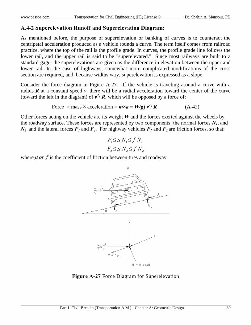
www.passpe.com Transportation for Civil Engineering (PE) License © Dr. Shahin A. Mansour, PE
Part I- Civil Breadth (Transportation A.M.) - Chapter A: Geometric Design 89
A.4-2 Superelevation Runoff and Superelevation Diagram:
As mentioned before, the purpose of superelevation or banking of curves is to counteract the centripetal acceleration produced as a vehicle rounds a curve. The term itself comes from railroad practice, where the top of the rail is the profile grade. In curves, the profile grade line follows the lower rail, and the upper rail is said to be "superelevated." Since most railways are built to a standard gage, the superelevations are given as the difference in elevation between the upper and lower rail. In the case of highways, somewhat more complicated modifications of the cross section are required, and, because widths vary, superelevation is expressed as a slope.
Consider the force diagram in Figure A-27. If the vehicle is traveling around a curve with a radius R at a constant speed v, there will be a radial acceleration toward the center of the curve (toward the left in the diagram) of v2/ R, which will be opposed by a force of:
Force = mass × acceleration = m×a = W/g) v2/ R (A-42)
Other forces acting on the vehicle are its weight W and the forces exerted against the wheels by the roadway surface. These forces are represented by two components: the normal forces N1, and N2 and the lateral forces F1 and F2. For highway vehicles F1 and F2 are friction forces, so that:
111 NfNF ≤≤ µ
222 NfNF ≤≤ µ where forµ is the coefficient of friction between tires and roadway.
Figure A-27 Force Diagram for Superelevation
www.passpe.com Transportation for Civil PE License © Dr. Shahin A.Mansour, PE
Part I- Civil Breadth (Transportation A.M.) - Chapter A: Geometric Design 90
In order to construct the superelevation diagram, the following parameters must be determined:
1- Axis of Rotation 2- Superelevation Transition
1- Axis of Rotation
(a) Undivided Highways:
For undivided highways the axis of rotation for superelevation is usually the centerline of the roadbed. However, in special cases such as desert roads where curves are preceded by long relatively level tangents, the plane of superelevation may be rotated about the inside edge of traveled way to improve perception of the curve. In flat country, drainage pockets caused by superelevation may be avoided by changing the axis of rotation from the centerline to the inside edge of traveled way.
(b) Ramps and Freeway-to-freeway Connections:
The axis of rotation may be about either edge of traveled way or centerline if multilane. Appearance and drainage considerations should always be taken into account in selection of the axis of rotation.
(c) Divided Highways.
(i) Freeways-Where the initial median width is 65 feet or less, the axis of rotation should be at the centerline.
Where the initial median width is greater than 65 feet and the ultimate median width is 65
feet or less, the axis of rotation should be at the centerline, except where the resulting initial median slope would be steeper than 10: 1. In the latter case, the axis of rotation should be at the ultimate median edges of traveled way.
Where the ultimate median width is greater than 65 feet, the axis of rotation should
normally be at the ultimate median edges of traveled way. To avoid sawtooth on bridges with decked medians, the axis of rotation, if not already on centerline, should be shifted to the centerline.
(ii) Conventional Highways-The axis of rotation should be considered on an individual project basis and the most appropriate case for the conditions should
2- Superelevation Transition:
The superelevation transition generally consists of the crown runoff and the superelevation runoff as shown on Figure A-28.
A superelevation transition should be designed to satisfy the requirements of safety, comfort and pleasing appearance. The length of superelevation transition should be based upon the combination of superelevation rate and width of rotated plane.
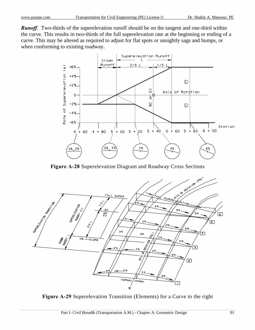
www.passpe.com Transportation for Civil Engineering (PE) License © Dr. Shahin A. Mansour, PE
Part I- Civil Breadth (Transportation A.M.) - Chapter A: Geometric Design 91
Runoff. Two-thirds of the superelevation runoff should be on the tangent and one-third within the curve. This results in two-thirds of the full superelevation rate at the beginning or ending of a curve. This may be altered as required to adjust for flat spots or unsightly sags and humps, or when conforming to existing roadway.
Figure A-28 Superelevation Diagram and Roadway Cross Sections
Figure A-29 Superelevation Transition (Elements) for a Curve to the right
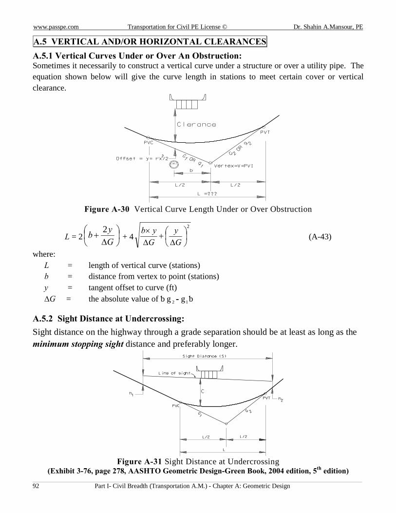
www.passpe.com Transportation for Civil PE License © Dr. Shahin A.Mansour, PE
Part I- Civil Breadth (Transportation A.M.) - Chapter A: Geometric Design 92
A.5 VERTICAL AND/OR HORIZONTAL CLEARANCES
A.5.1 Vertical Curves Under or Over An Obstruction: Sometimes it necessarily to construct a vertical curve under a structure or over a utility pipe. The equation shown below will give the curve length in stations to meet certain cover or vertical clearance.
Figure A-30 Vertical Curve Length Under or Over Obstruction
L = 2
∆+
Gyb 2
+ 42
∆+
∆×
Gy
Gyb
(A-43)
where: L = length of vertical curve (stations) b = distance from vertex to point (stations) y = tangent offset to curve (ft) ∆G = the absolute value of │g 2 - g1│
A.5.2 Sight Distance at Undercrossing:
Sight distance on the highway through a grade separation should be at least as long as the minimum stopping sight distance and preferably longer.
Figure A-31 Sight Distance at Undercrossing
(Exhibit 3-76, page 278, AASHTO Geometric Design-Green Book, 2004 edition, 5th edition)
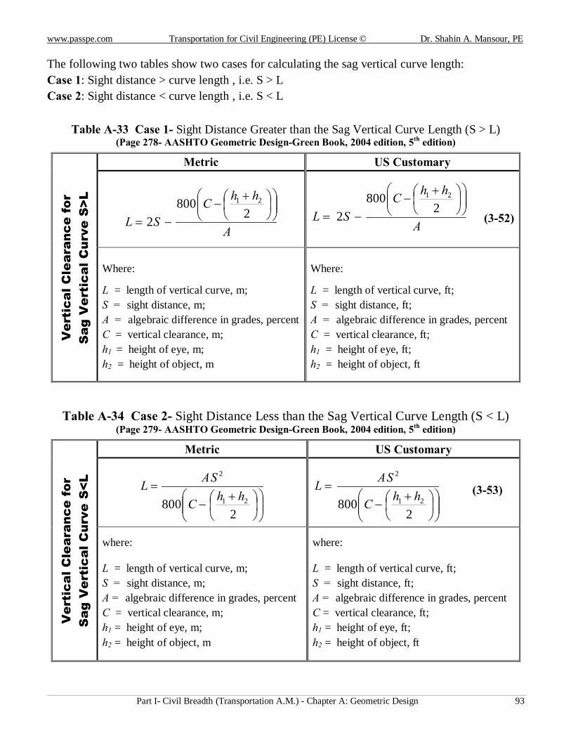
www.passpe.com Transportation for Civil Engineering (PE) License © Dr. Shahin A. Mansour, PE
Part I- Civil Breadth (Transportation A.M.) - Chapter A: Geometric Design 93
The following two tables show two cases for calculating the sag vertical curve length: Case 1: Sight distance > curve length , i.e. S > L Case 2: Sight distance < curve length , i.e. S < L
Table A-33 Case 1- Sight Distance Greater than the Sag Vertical Curve Length (S > L) (Page 278- AASHTO Geometric Design-Green Book, 2004 edition, 5th edition)
Ver
tica
l Cle
aran
ce f
or
Sag
Ver
tica
l Cur
ve S
>L
Metric US Customary
A
hhCSL
+
−−=
2800
2
21
A
hhCSL
+
−−=
2800
2
21
(3-52)
Where: L = length of vertical curve, m; S = sight distance, m; A = algebraic difference in grades, percent C = vertical clearance, m; h1 = height of eye, m; h2 = height of object, m
Where: L = length of vertical curve, ft; S = sight distance, ft; A = algebraic difference in grades, percent C = vertical clearance, ft; h1 = height of eye, ft; h2 = height of object, ft
Table A-34 Case 2- Sight Distance Less than the Sag Vertical Curve Length (S < L) (Page 279- AASHTO Geometric Design-Green Book, 2004 edition, 5th edition)
Ver
tica
l Cle
aran
ce f
or
Sag
Ver
tica
l Cur
ve S
<L
Metric US Customary
+
−=
2800 21
2
hhC
SAL
+
−=
2800 21
2
hhC
SAL (3-53)
where: L = length of vertical curve, m; S = sight distance, m; A = algebraic difference in grades, percent C = vertical clearance, m; h1 = height of eye, m; h2 = height of object, m
where: L = length of vertical curve, ft; S = sight distance, ft; A = algebraic difference in grades, percent C = vertical clearance, ft; h1 = height of eye, ft; h2 = height of object, ft
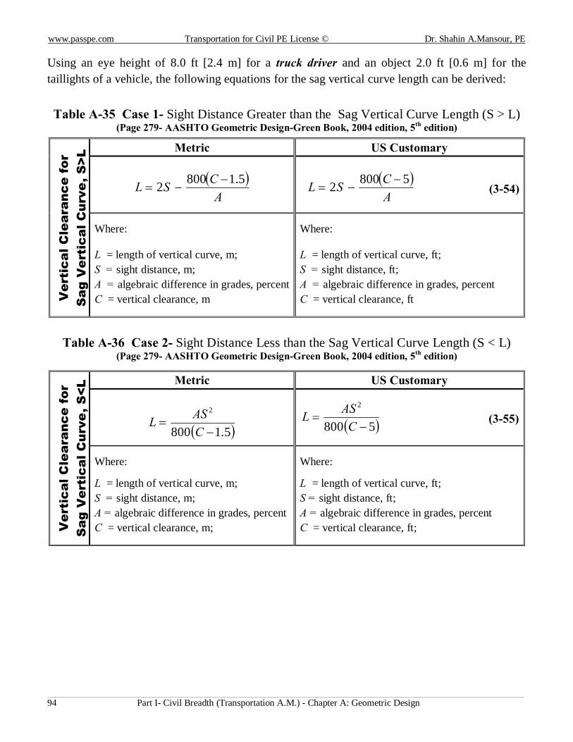
www.passpe.com Transportation for Civil PE License © Dr. Shahin A.Mansour, PE
Part I- Civil Breadth (Transportation A.M.) - Chapter A: Geometric Design 94
Using an eye height of 8.0 ft [2.4 m] for a truck driver and an object 2.0 ft [0.6 m] for the taillights of a vehicle, the following equations for the sag vertical curve length can be derived:
Table A-35 Case 1- Sight Distance Greater than the Sag Vertical Curve Length (S > L) (Page 279- AASHTO Geometric Design-Green Book, 2004 edition, 5th edition)
Ver
tica
l Cle
aran
ce f
or
Sag
Ver
tica
l Cur
ve, S
>L Metric US Customary
( )
ACSL 5.18002 −
−=
( )ACSL 58002 −
−= (3-54)
Where: L = length of vertical curve, m; S = sight distance, m; A = algebraic difference in grades, percent C = vertical clearance, m
Where: L = length of vertical curve, ft; S = sight distance, ft; A = algebraic difference in grades, percent C = vertical clearance, ft
Table A-36 Case 2- Sight Distance Less than the Sag Vertical Curve Length (S < L) (Page 279- AASHTO Geometric Design-Green Book, 2004 edition, 5th edition)
Ver
tica
l Cle
aran
ce f
or
Sag
Ver
tica
l Cur
ve, S
<L Metric US Customary
( )5.1800
2
−=
CASL
( )5800
2
−=
CASL (3-55)
Where: L = length of vertical curve, m; S = sight distance, m; A = algebraic difference in grades, percent C = vertical clearance, m;
Where: L = length of vertical curve, ft; S = sight distance, ft; A = algebraic difference in grades, percent C = vertical clearance, ft;
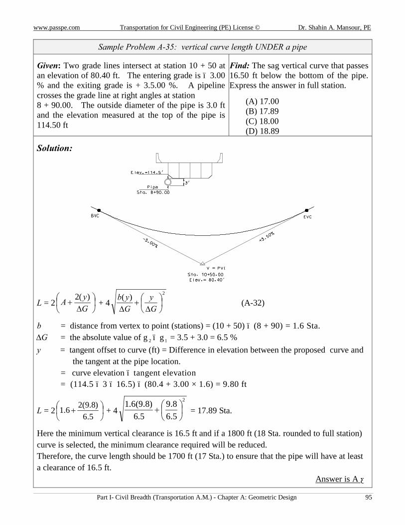
www.passpe.com Transportation for Civil Engineering (PE) License © Dr. Shahin A. Mansour, PE
Part I- Civil Breadth (Transportation A.M.) - Chapter A: Geometric Design 95
Sample Problem A-35: vertical curve length UNDER a pipe
Given: Two grade lines intersect at station 10 + 50 at an elevation of 80.40 ft. The entering grade is – 3.00 % and the exiting grade is + 3.5.00 %. A pipeline crosses the grade line at right angles at station 8 + 90.00. The outside diameter of the pipe is 3.0 ft and the elevation measured at the top of the pipe is 114.50 ft
Find: The sag vertical curve that passes 16.50 ft below the bottom of the pipe. Express the answer in full station.
(A) 17.00 (B) 17.89 (C) 18.00 (D) 18.89
Solution:
L = 2
∆+
GyA )(2
+ 42)(
∆+
∆ Gy
Gyb
(A-32)
b = distance from vertex to point (stations) = (10 + 50) – (8 + 90) = 1.6 Sta. ∆G = the absolute value of g 2 – g1 = 3.5 + 3.0 = 6.5 % y = tangent offset to curve (ft) = Difference in elevation between the proposed curve and
the tangent at the pipe location. = curve elevation – tangent elevation = (114.5 – 3 – 16.5) – (80.4 + 3.00 × 1.6) = 9.80 ft
L = 2
+
5.6)8.9(26.1 + 4
2
5.68.9
5.6)8.9(6.1
+ = 17.89 Sta.
Here the minimum vertical clearance is 16.5 ft and if a 1800 ft (18 Sta. rounded to full station) curve is selected, the minimum clearance required will be reduced. Therefore, the curve length should be 1700 ft (17 Sta.) to ensure that the pipe will have at least a clearance of 16.5 ft.
Answer is A ◄
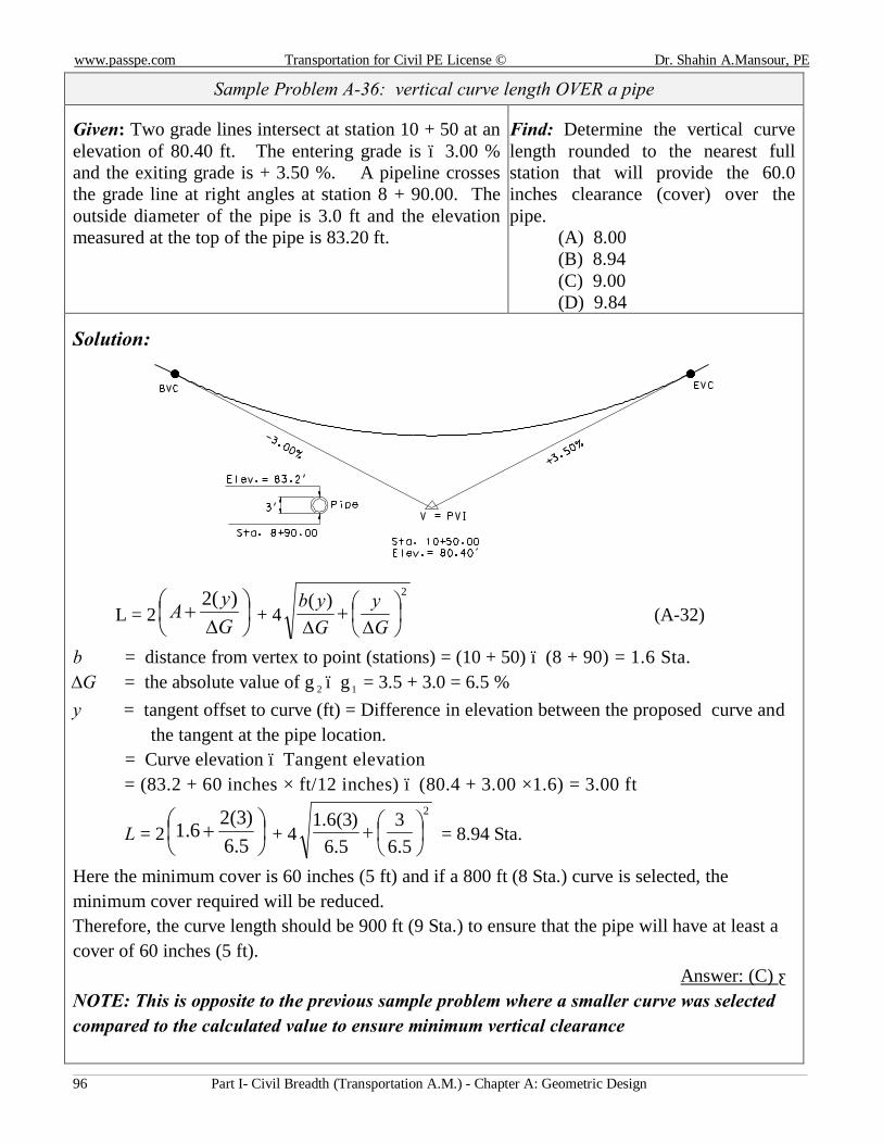
www.passpe.com Transportation for Civil PE License © Dr. Shahin A.Mansour, PE
Part I- Civil Breadth (Transportation A.M.) - Chapter A: Geometric Design 96
Sample Problem A-36: vertical curve length OVER a pipe
Given: Two grade lines intersect at station 10 + 50 at an elevation of 80.40 ft. The entering grade is – 3.00 % and the exiting grade is + 3.50 %. A pipeline crosses the grade line at right angles at station 8 + 90.00. The outside diameter of the pipe is 3.0 ft and the elevation measured at the top of the pipe is 83.20 ft.
Find: Determine the vertical curve length rounded to the nearest full station that will provide the 60.0 inches clearance (cover) over the pipe.
(A) 8.00 (B) 8.94 (C) 9.00 (D) 9.84
Solution:
L = 2
∆+
GyA )(2
+ 42)(
∆+
∆ Gy
Gyb
(A-32)
b = distance from vertex to point (stations) = (10 + 50) – (8 + 90) = 1.6 Sta. ∆G = the absolute value of g 2 – g1 = 3.5 + 3.0 = 6.5 % y = tangent offset to curve (ft) = Difference in elevation between the proposed curve and
the tangent at the pipe location. = Curve elevation – Tangent elevation = (83.2 + 60 inches × ft/12 inches) – (80.4 + 3.00 ×1.6) = 3.00 ft
L = 2
+
5.6)3(26.1 + 4
2
5.63
5.6)3(6.1
+ = 8.94 Sta.
Here the minimum cover is 60 inches (5 ft) and if a 800 ft (8 Sta.) curve is selected, the minimum cover required will be reduced. Therefore, the curve length should be 900 ft (9 Sta.) to ensure that the pipe will have at least a cover of 60 inches (5 ft).
Answer: (C) ◄ NOTE: This is opposite to the previous sample problem where a smaller curve was selected compared to the calculated value to ensure minimum vertical clearance
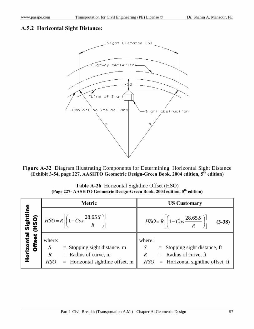
www.passpe.com Transportation for Civil Engineering (PE) License © Dr. Shahin A. Mansour, PE
Part I- Civil Breadth (Transportation A.M.) - Chapter A: Geometric Design 97
A.5.2 Horizontal Sight Distance:
Figure A-32 Diagram Illustrating Components for Determining Horizontal Sight Distance (Exhibit 3-54, page 227, AASHTO Geometric Design-Green Book, 2004 edition, 5th edition)
Table A-26 Horizontal Sightline Offset (HSO)
(Page 227- AASHTO Geometric Design-Green Book, 2004 edition, 5th edition)
Hor
izon
tal S
ight
line
Off
set
(HS
O)
Metric US Customary
−=
RSCosRHSO 65.281
−=
RSCosRHSO 65.281 (3-38)
where: S = Stopping sight distance, m R = Radius of curve, m HSO = Horizontal sightline offset, m
where: S = Stopping sight distance, ft R = Radius of curve, ft HSO = Horizontal sightline offset, ft
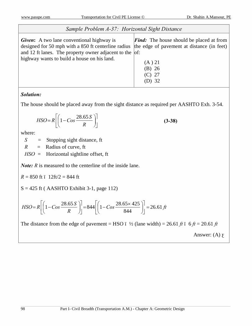
www.passpe.com Transportation for Civil PE License © Dr. Shahin A.Mansour, PE
Part I- Civil Breadth (Transportation A.M.) - Chapter A: Geometric Design 98
Sample Problem A-37: Horizontal Sight Distance
Given: A two lane conventional highway is designed for 50 mph with a 850 ft centerline radius and 12 ft lanes. The property owner adjacent to the highway wants to build a house on his land.
Find: The house should be placed at from the edge of pavement at distance (in feet) of:
(A ) 21 (B) 26 (C) 27 (D) 32
Solution:
The house should be placed away from the sight distance as required per AASHTO Exh. 3-54.
−=
RSCosRHSO 65.281 (3-38)
where: S = Stopping sight distance, ft R = Radius of curve, ft HSO = Horizontal sightline offset, ft
Note: R is measured to the centerline of the inside lane.
R = 850 ft − 12ft/2 = 844 ft
S = 425 ft ( AASHTO Exhibit 3-1, page 112)
ftCosR
SCosRHSO 61.26844
42565.28184465.281 =
×
−=
−=
The distance from the edge of pavement = HSO − ½ (lane width) = 26.61 ft − 6 ft = 20.61 ft
Answer: (A) ◄
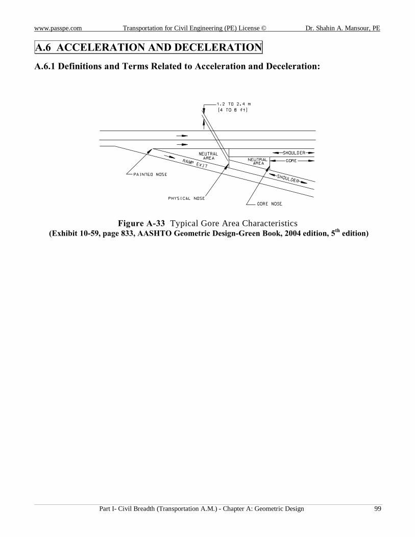
www.passpe.com Transportation for Civil Engineering (PE) License © Dr. Shahin A. Mansour, PE
Part I- Civil Breadth (Transportation A.M.) - Chapter A: Geometric Design 99
A.6 ACCELERATION AND DECELERATION
A.6.1 Definitions and Terms Related to Acceleration and Deceleration:
Figure A-33 Typical Gore Area Characteristics (Exhibit 10-59, page 833, AASHTO Geometric Design-Green Book, 2004 edition, 5th edition)
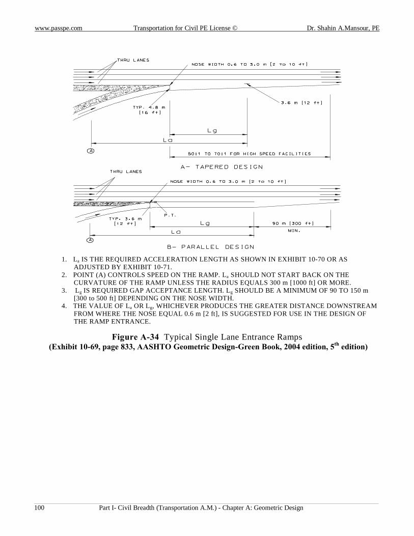
www.passpe.com Transportation for Civil PE License © Dr. Shahin A.Mansour, PE
Part I- Civil Breadth (Transportation A.M.) - Chapter A: Geometric Design 100
1. La IS THE REQUIRED ACCELERATION LENGTH AS SHOWN IN EXHIBIT 10-70 OR AS ADJUSTED BY EXHIBIT 10-71.
2. POINT (A) CONTROLS SPEED ON THE RAMP. La SHOULD NOT START BACK ON THE CURVATURE OF THE RAMP UNLESS THE RADIUS EQUALS 300 m [1000 ft] OR MORE.
3. Lg IS REQUIRED GAP ACCEPTANCE LENGTH. Lg SHOULD BE A MINIMUM OF 90 TO 150 m [300 to 500 ft] DEPENDING ON THE NOSE WIDTH.
4. THE VALUE OF La OR Lg, WHICHEVER PRODUCES THE GREATER DISTANCE DOWNSTREAM FROM WHERE THE NOSE EQUAL 0.6 m [2 ft], IS SUGGESTED FOR USE IN THE DESIGN OF THE RAMP ENTRANCE.
Figure A-34 Typical Single Lane Entrance Ramps (Exhibit 10-69, page 833, AASHTO Geometric Design-Green Book, 2004 edition, 5th edition)
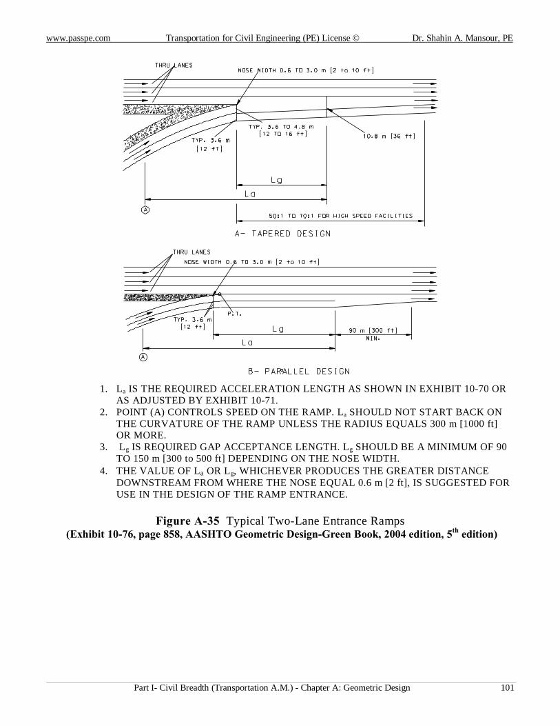
www.passpe.com Transportation for Civil Engineering (PE) License © Dr. Shahin A. Mansour, PE
Part I- Civil Breadth (Transportation A.M.) - Chapter A: Geometric Design 101
1. La IS THE REQUIRED ACCELERATION LENGTH AS SHOWN IN EXHIBIT 10-70 OR AS ADJUSTED BY EXHIBIT 10-71.
2. POINT (A) CONTROLS SPEED ON THE RAMP. La SHOULD NOT START BACK ON THE CURVATURE OF THE RAMP UNLESS THE RADIUS EQUALS 300 m [1000 ft] OR MORE.
3. Lg IS REQUIRED GAP ACCEPTANCE LENGTH. Lg SHOULD BE A MINIMUM OF 90 TO 150 m [300 to 500 ft] DEPENDING ON THE NOSE WIDTH.
4. THE VALUE OF La OR Lg, WHICHEVER PRODUCES THE GREATER DISTANCE DOWNSTREAM FROM WHERE THE NOSE EQUAL 0.6 m [2 ft], IS SUGGESTED FOR USE IN THE DESIGN OF THE RAMP ENTRANCE.
Figure A-35 Typical Two-Lane Entrance Ramps
(Exhibit 10-76, page 858, AASHTO Geometric Design-Green Book, 2004 edition, 5th edition)
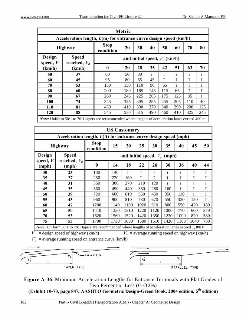
www.passpe.com Transportation for Civil PE License © Dr. Shahin A.Mansour, PE
Part I- Civil Breadth (Transportation A.M.) - Chapter A: Geometric Design 102
Metric Acceleration length, L(m) for entrance curve design speed (km/h)
Highway Stop condition 20 30 40 50 60 70 80
Design speed, V (km/h)
Speed reached, Va
(km/h)
and initial speed, aV ′ (km/h)
0 20 28 35 42 51 63 70 50 37 60 50 30 − − − − − 60 45 95 80 65 45 − − − − 70 53 150 130 110 90 65 − − − 80 60 200 180 165 145 115 65 − − 90 67 260 245 225 205 175 125 35 − 100 74 345 325 305 285 255 205 110 40 110 81 430 410 390 370 340 290 200 125 120 88 545 530 515 490 460 410 325 245
Note: Uniform 50:1 to 70:1 tapers are recommended where lengths of acceleration lanes exceed 400 m.
US Customary Acceleration length, L(ft) for entrance curve design speed (mph)
Highway Stop condition 15 20 25 30 35 40 45 50
Design speed, V (mph)
Speed reached, Va
(mph)
and initial speed, aV ′ (mph)
0 14 18 22 26 30 36 40 44 30 23 180 140 − − − − − − − 35 27 280 220 160 − − − − − − 40 31 360 300 270 210 120 − − − − 45 35 560 490 440 380 280 160 − − − 50 39 720 660 610 550 450 350 130 − − 55 43 960 900 810 780 670 550 320 150 − 60 47 1200 1140 1100 1020 910 800 550 420 180 65 50 1410 1350 1310 1220 1120 1000 770 600 370 70 53 1620 1560 1520 1420 1350 1230 1000 820 580 75 55 1790 1730 1630 1580 1510 1420 1160 1040 780
Note: Uniform 50:1 to 70:1 tapers are recommended where lengths of acceleration lanes exceed 1,300 ft V = design speed of highway (km/h) Va = average running speed on highway (km/h) aV ′ = average running speed on entrance curve (km/h)
Figure A-36 Minimum Acceleration Lengths for Entrance Terminals with Flat Grades of Two Percent or Less (G ≤ 2%)
(Exhibit 10-70, page 847, AASHTO Geometric Design-Green Book, 2004 edition, 5th edition)
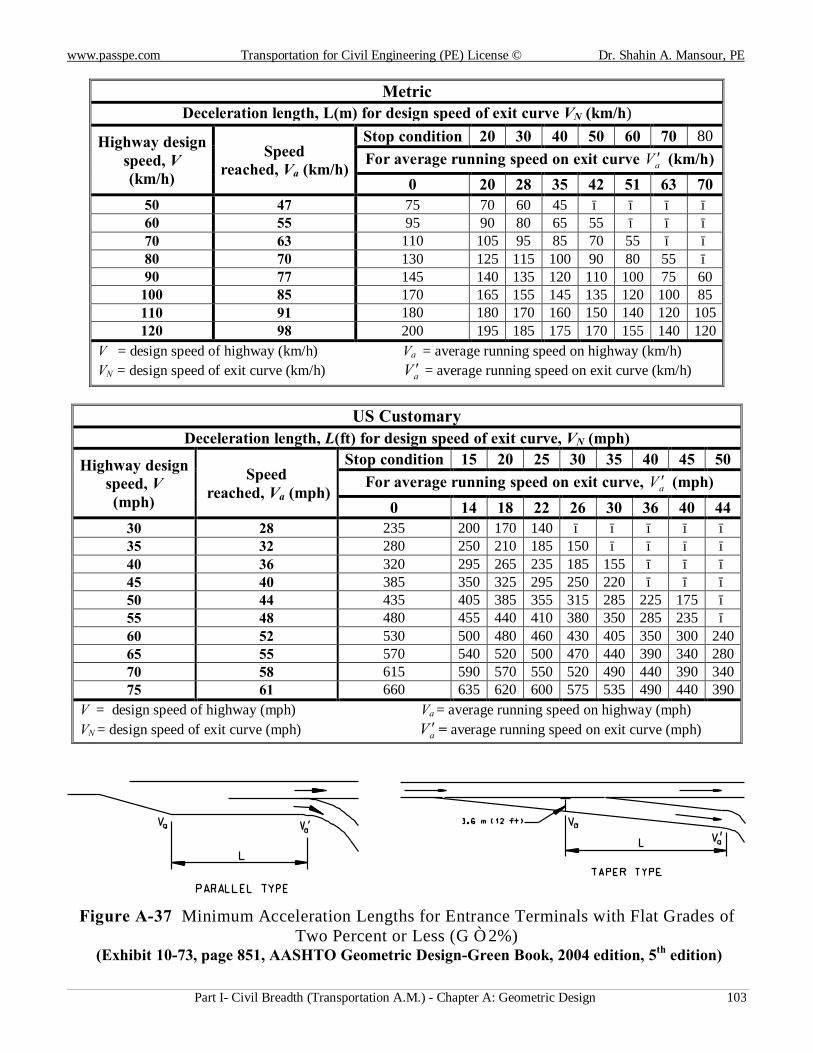
www.passpe.com Transportation for Civil Engineering (PE) License © Dr. Shahin A. Mansour, PE
Part I- Civil Breadth (Transportation A.M.) - Chapter A: Geometric Design 103
Metric Deceleration length, L(m) for design speed of exit curve VN (km/h)
Highway design speed, V (km/h)
Speed reached, Va (km/h)
Stop condition 20 30 40 50 60 70 80 For average running speed on exit curve aV ′ (km/h)
0 20 28 35 42 51 63 70 50 47 75 70 60 45 − − − − 60 55 95 90 80 65 55 − − − 70 63 110 105 95 85 70 55 − − 80 70 130 125 115 100 90 80 55 − 90 77 145 140 135 120 110 100 75 60
100 85 170 165 155 145 135 120 100 85 110 91 180 180 170 160 150 140 120 105 120 98 200 195 185 175 170 155 140 120
V = design speed of highway (km/h) Va = average running speed on highway (km/h) VN = design speed of exit curve (km/h) aV ′ = average running speed on exit curve (km/h)
US Customary
Deceleration length, L(ft) for design speed of exit curve, VN (mph)
Highway design speed, V (mph)
Speed reached, Va (mph)
Stop condition 15 20 25 30 35 40 45 50 For average running speed on exit curve, aV ′ (mph)
0 14 18 22 26 30 36 40 44 30 28 235 200 170 140 − − − − − 35 32 280 250 210 185 150 − − − − 40 36 320 295 265 235 185 155 − − − 45 40 385 350 325 295 250 220 − − − 50 44 435 405 385 355 315 285 225 175 − 55 48 480 455 440 410 380 350 285 235 − 60 52 530 500 480 460 430 405 350 300 240 65 55 570 540 520 500 470 440 390 340 280 70 58 615 590 570 550 520 490 440 390 340 75 61 660 635 620 600 575 535 490 440 390
V = design speed of highway (mph) Va = average running speed on highway (mph) VN = design speed of exit curve (mph) aV ′ = average running speed on exit curve (mph)
Figure A-37 Minimum Acceleration Lengths for Entrance Terminals with Flat Grades of Two Percent or Less (G ≤ 2%)
(Exhibit 10-73, page 851, AASHTO Geometric Design-Green Book, 2004 edition, 5th edition)
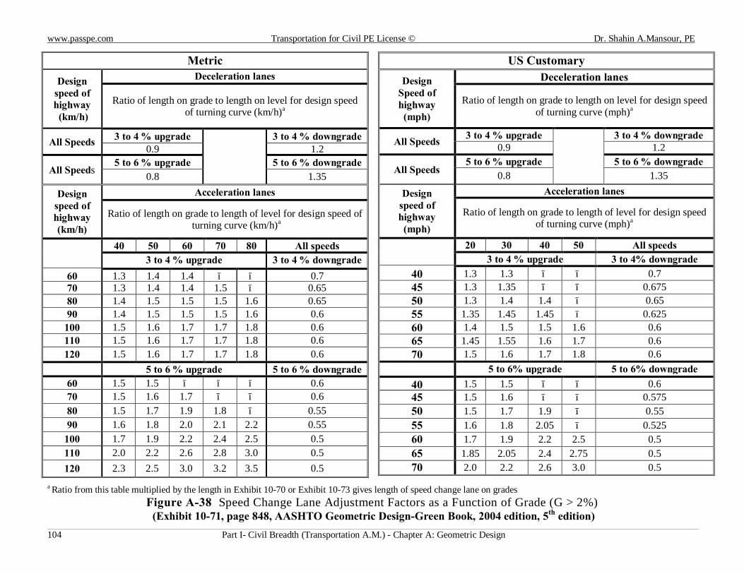
www.passpe.com Transportation for Civil PE License © Dr. Shahin A.Mansour, PE
Part I- Civil Breadth (Transportation A.M.) - Chapter A: Geometric Design 104
a Ratio from this table multiplied by the length in Exhibit 10-70 or Exhibit 10-73 gives length of speed change lane on grades
Figure A-38 Speed Change Lane Adjustment Factors as a Function of Grade (G > 2%) (Exhibit 10-71, page 848, AASHTO Geometric Design-Green Book, 2004 edition, 5th edition)
Metric Design
speed of highway (km/h)
Deceleration lanes
Ratio of length on grade to length on level for design speed of turning curve (km/h)a
All Speeds 3 to 4 % upgrade
3 to 4 % downgrade 0.9 1.2
All Speeds 5 to 6 % upgrade 5 to 6 % downgrade
0.8 1.35
Design speed of highway (km/h)
Acceleration lanes
Ratio of length on grade to length of level for design speed of turning curve (km/h)a
40 50 60 70 80 All speeds 3 to 4 % upgrade 3 to 4 % downgrade
60 1.3 1.4 1.4 − − 0.7 70 1.3 1.4 1.4 1.5 − 0.65 80 1.4 1.5 1.5 1.5 1.6 0.65 90 1.4 1.5 1.5 1.5 1.6 0.6
100 1.5 1.6 1.7 1.7 1.8 0.6 110 1.5 1.6 1.7 1.7 1.8 0.6 120 1.5 1.6 1.7 1.7 1.8 0.6
5 to 6 % upgrade 5 to 6 % downgrade 60 1.5 1.5 − − − 0.6 70 1.5 1.6 1.7 − − 0.6 80 1.5 1.7 1.9 1.8 − 0.55 90 1.6 1.8 2.0 2.1 2.2 0.55
100 1.7 1.9 2.2 2.4 2.5 0.5 110 2.0 2.2 2.6 2.8 3.0 0.5 120 2.3 2.5 3.0 3.2 3.5 0.5
US Customary Design
Speed of highway (mph)
Deceleration lanes
Ratio of length on grade to length on level for design speed of turning curve (mph)a
All Speeds 3 to 4 % upgrade
3 to 4 % downgrade 0.9 1.2
All Speeds 5 to 6 % upgrade 5 to 6 % downgrade
0.8 1.35
Design speed of highway (mph)
Acceleration lanes
Ratio of length on grade to length of level for design speed of turning curve (mph)a
20 30 40 50 All speeds 3 to 4 % upgrade 3 to 4% downgrade
40 1.3 1.3 − − 0.7 45 1.3 1.35 − − 0.675 50 1.3 1.4 1.4 − 0.65 55 1.35 1.45 1.45 − 0.625 60 1.4 1.5 1.5 1.6 0.6 65 1.45 1.55 1.6 1.7 0.6 70 1.5 1.6 1.7 1.8 0.6 5 to 6% upgrade 5 to 6% downgrade
40 1.5 1.5 − − 0.6 45 1.5 1.6 − − 0.575 50 1.5 1.7 1.9 − 0.55 55 1.6 1.8 2.05 − 0.525 60 1.7 1.9 2.2 2.5 0.5 65 1.85 2.05 2.4 2.75 0.5 70 2.0 2.2 2.6 3.0 0.5
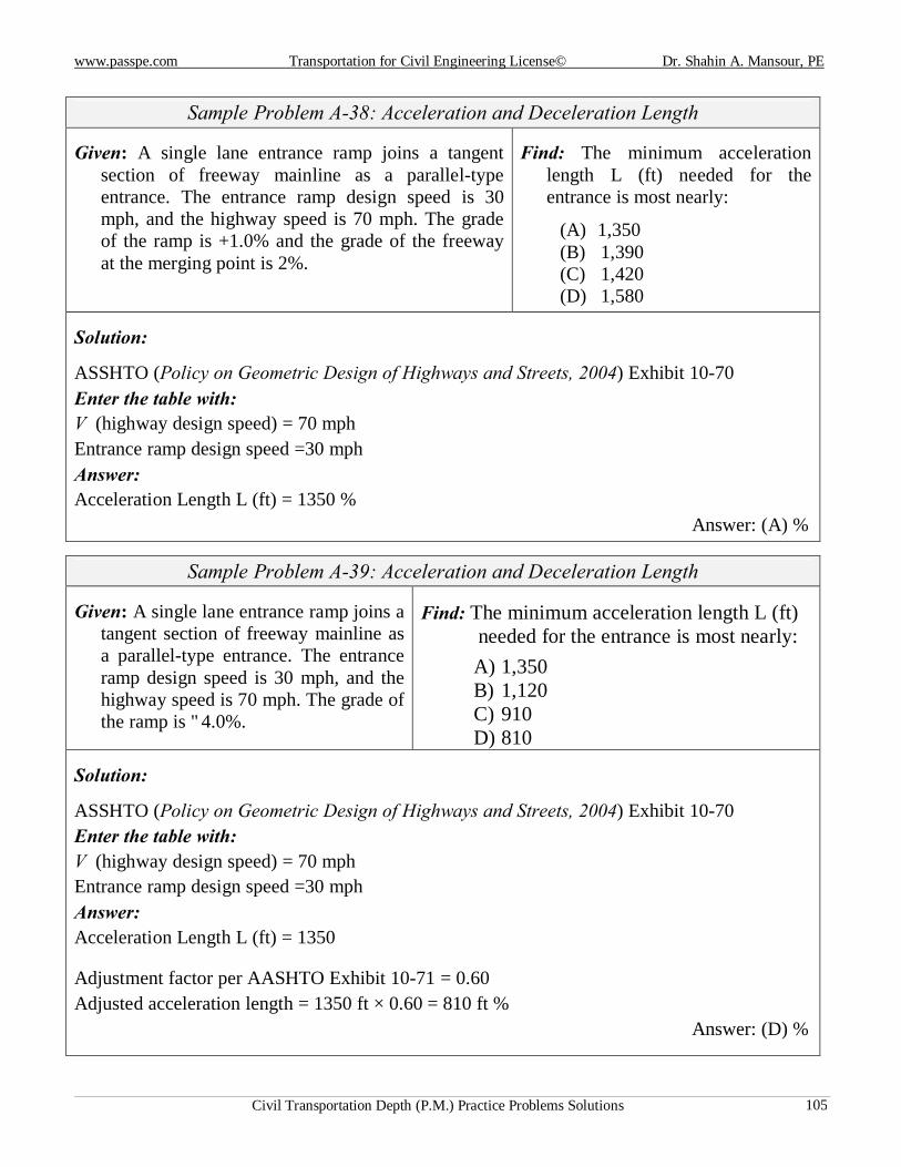
www.passpe.com Transportation for Civil Engineering License© Dr. Shahin A. Mansour, PE
Civil Transportation Depth (P.M.) Practice Problems Solutions 105
Sample Problem A-38: Acceleration and Deceleration Length
Given: A single lane entrance ramp joins a tangent section of freeway mainline as a parallel-type entrance. The entrance ramp design speed is 30 mph, and the highway speed is 70 mph. The grade of the ramp is +1.0% and the grade of the freeway at the merging point is 2%.
Find: The minimum acceleration length L (ft) needed for the entrance is most nearly:
(A) 1,350 (B) 1,390 (C) 1,420 (D) 1,580
Solution:
ASSHTO (Policy on Geometric Design of Highways and Streets, 2004) Exhibit 10-70 Enter the table with: V (highway design speed) = 70 mph Entrance ramp design speed =30 mph Answer: Acceleration Length L (ft) = 1350 ◄
Answer: (A) ◄
Sample Problem A-39: Acceleration and Deceleration Length
Given: A single lane entrance ramp joins a tangent section of freeway mainline as a parallel-type entrance. The entrance ramp design speed is 30 mph, and the highway speed is 70 mph. The grade of the ramp is −4.0%.
Find: The minimum acceleration length L (ft) needed for the entrance is most nearly:
A) 1,350 B) 1,120 C) 910 D) 810
Solution:
ASSHTO (Policy on Geometric Design of Highways and Streets, 2004) Exhibit 10-70 Enter the table with: V (highway design speed) = 70 mph Entrance ramp design speed =30 mph Answer: Acceleration Length L (ft) = 1350
Adjustment factor per AASHTO Exhibit 10-71 = 0.60 Adjusted acceleration length = 1350 ft × 0.60 = 810 ft ◄
Answer: (D) ◄
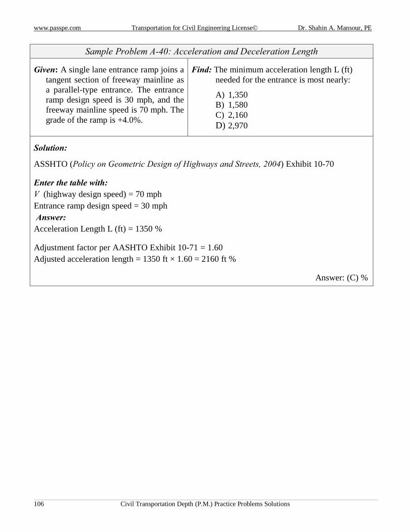
www.passpe.com Transportation for Civil Engineering License© Dr. Shahin A. Mansour, PE
Civil Transportation Depth (P.M.) Practice Problems Solutions 106
Sample Problem A-40: Acceleration and Deceleration Length
Given: A single lane entrance ramp joins a tangent section of freeway mainline as a parallel-type entrance. The entrance ramp design speed is 30 mph, and the freeway mainline speed is 70 mph. The grade of the ramp is +4.0%.
Find: The minimum acceleration length L (ft) needed for the entrance is most nearly:
A) 1,350 B) 1,580 C) 2,160 D) 2,970
Solution:
ASSHTO (Policy on Geometric Design of Highways and Streets, 2004) Exhibit 10-70
Enter the table with: V (highway design speed) = 70 mph Entrance ramp design speed = 30 mph Answer: Acceleration Length L (ft) = 1350 ◄
Adjustment factor per AASHTO Exhibit 10-71 = 1.60 Adjusted acceleration length = 1350 ft × 1.60 = 2160 ft ◄
Answer: (C) ◄
www.passpe.com Transportation for Civil Engineering License© Dr. Shahin A. Mansour, PE
Civil Transportation Depth (P.M.) Practice Problems Solutions 107