Transportation Research Part C 20 (2012) 164–184

Contents lists available at ScienceDirect

Transportation Research Part C

journal homepage: www.elsevier .com/locate / t rc

PAMSCOD: Platoon-based arterial multi-modal signal controlwith online data

Qing He, K. Larry Head ⇑, Jun DingUniversity of Arizona, Tucson, AZ 85721, USA

a r t i c l e i n f o

Keywords:Multi-modal traffic signal controlPlatoon recognitionMixed integer linear programmingMulti-modal dynamical progressionVehicle-to-infrastructure communications

0968-090X/$ - see front matter � 2011 Elsevier Ltddoi:10.1016/j.trc.2011.05.007

⇑ Corresponding author. Tel.: +1 520 621 2264; faE-mail address: larry@sie.arizona.edu (K.L. Head

a b s t r a c t

A unified platoon-based mathematical formulation called PAMSCOD is presented to per-form arterial (network) traffic signal control while considering multiple travel modes ina vehicle-to-infrastructure communications environment. First, a headway-based platoonrecognition algorithm is developed to identify pseudo-platoons given probe vehicles’online information. It is assumed that passenger vehicles constitute a significant majorityof the vehicles in the network. This algorithm identifies existing queues and significant pla-toons approaching each intersection. Second, a mixed-integer linear program (MILP) issolved to determine future optimal signal plans based on the current traffic controller sta-tus, online platoon data and priority requests from special vehicles, such as transit buses.Deviating from the traditional common network cycle length, PAMSCOD aims to providemulti-modal dynamical progression (MDP) on the arterial based on the probe information.Microscopic simulation using VISSIM shows that PAMSCOD can easily handle two commontraffic modes, transit buses and automobiles, and significantly reduce delays for bothmodes under both non-saturated and oversaturated traffic conditions as compared to tra-ditional state-of-practice coordinated-actuated signal control with timings optimized bySYNCHRO.

� 2011 Elsevier Ltd. All rights reserved.

1. Introduction

Traffic signals are very important tools for urban traffic management. With correct installation and control strategy selec-tion, they can improve both traffic throughput and safety for all road users. Traffic flow usually consists of more than onetravel mode, including automobiles, transit buses, and emergency vehicles as well as commercial trucks, bicycles, and pedes-trians. Different travel modes have their own specific characteristics, including travel speed, density, and priority level. Tra-ditionally, traffic operations treat different travel modes separately (e.g., signal coordination for automobiles, signalpreemption for emergency vehicles, and transit signal priority (TSP) for buses). However, treating each mode separately islikely to result in sub-optimal performance. In the environment of vehicle-to-infrastructure communications (Researchand Innovative Technology Administration, 2011), enriched traffic data makes optimal multi-modal traffic control a real pos-sibility. Systems of traffic signals, such as along an arterial, need to be coordinated based on actual traffic composition andthe flow of vehicles. With the advent of vehicle-based positioning and communications, it is possible to know where vehiclesare and to plan traffic signal control to best serve all vehicles in the entire network.

This paper presents a unified platoon-based formulation called Platoon-based Arterial Multi-modal Signal Controlwith Online Data (PAMSCOD) to concurrently optimize network traffic signal control for different travel modes given the

. All rights reserved.

x: +1 520 621 6555.).

Q. He et al. / Transportation Research Part C 20 (2012) 164–184 165

assumption that advanced communication systems are available between vehicles and traffic controllers. In this paper, twomodes of traffic composition are considered: transit buses and passenger vehicles in a decision framework that can easilyaccommodate pedestrians and bicycles. First, when approaching an intersection, travelers are able to send a ‘‘green light’’ re-quest to the traffic controller. The ‘‘green light’’ request includes travelers’ travel mode, position, speed, and requested trafficsignal phase (which they know from a digital map of the intersection that contains the relevant information). Single requestsare categorized and clustered into platoons by priority level and phase. Finally, a mixed-integer linear program (MILP) issolved online for future optimal signal plans based on the real-time arterial platoon request data and traffic controller status.

One feature of PAMSCOD is network level dynamical signal coordination without the constraint of common cycle lengthand fixed offsets. State-of-the-practice coordinated-actuated control requires a common fixed cycle length and a predeter-mined set of offsets, which are generally developed only for automobiles under a certain range of traffic flow conditions.

In addition to the consideration of multi-modes, the large variance of traffic flow can degrade the performance of off-lineoptimized time-of-day plans (Yin, 2008). Robust traffic signal control is less sensitive to variances in traffic flow. To achieveboth robust and multi-modal network traffic signal control, the concept of multi-modal dynamical progression (MDP) is pro-posed in this paper. Regardless of cycle length and offsets, multi-modal dynamical progression along an arterial is realized inthe MILP formulation by adjusting phase durations to minimize the overall multi-modal delay both at the current intersec-tion and downstream intersections.

Large MILP formulations for signal control problems are subject to the ‘‘curse of dimensionality’’ and are not easily solvedin real-time (He et al., 2010). To address the issue of computational complexity, three measures are taken into account. First,the automobile requests are aggregated into platoons requesting specific phases to reduce the total number of integer vari-ables (from each individual vehicle to platoons of vehicles), as the number of integer variables contributes significantly to thecomplexity of the MILP formulation. Second, the integer feasible region is enhanced by assuming a first-come, first-serveddiscipline for the requests on the same approach. For example, suppose two platoons are requesting the same phase. The firstplatoon should always travel through the intersection before the second platoon. Third, multi-modal dynamical progressionis only considered between adjacent intersections due to the large variations of real-time traffic data. It is assumed that thecontrol problem can be resolved frequently to coordinate across time and space.

It is well known that traffic signal control is very difficult during oversaturated traffic conditions (Gazis, 1964). Oversat-urated traffic situations are caused by traffic demands that exceed the available capacity and can produce queues that growover time. Residual queues can overflow the storage capacity of urban streets and physically block intersections to cause defacto red (Abu-Lebdeh and Benekohal, 1997) when queue build-up leads to complete blockage of upstream signals and notraffic can discharge when the traffic signal is green. When real-time queue length and queue size are available from ad-vanced vehicle-based communications, the link capacity between adjacent intersections is known. Therefore, PAMSCOD isable to control the discharge rate from upstream intersections to avoid de facto red.

This paper is organized as follows. Section 2 presents a fast algorithm to identify platoons. Section 3 develops a MILP toaddress online arterial (or network) platoon-based multi-modal traffic signal control. Both dynamical progression and queuemanagement are discussed in this section. Section 4 compares the performance of PAMSCOD with different traffic signal con-trol methods under different traffic volume and scenarios. Section 5 presents a summary of the model and performancecomparison.

2. Platoon identification with probe vehicles

Many well-known traffic signal control algorithms have been based on platoon dynamics. Platoon dispersion and second-ary flows were considered in the TRANSYT-7F model (Robertson, 1969; Wallace et al., 1998) which has evolved into the wellknown adaptive traffic signal control system SCOOT (Hunt, 1982). Dell’Olmo and Mirchandani (1995) proposed a real-time,platoon-based network level control algorithm called REALBAND which attempts to resolve future platoon conflicts. REAL-BAND generates platoon information based on loop detector data (Gaur and Mirchandani, 2001) and creates a decision treebased on the projected platoon flow to find the best root-to-leaf decision by minimizing the total platoon delay. REALBANDhas been developed as one component of the RHODES adaptive traffic signal control system (Mirchandani and Head, 2001).Recently, a platoon-based traffic signal control algorithm was developed by Jiang et al. (2006) for intersections with major–minor traffic volume. However, their approach does not consider coordination as a primary consideration.

Traditional platoon recognition relies on pre-selected platoon detector locations. Platoons are identified by vehicle den-sity (Gaur and Mirchandani, 2001), cumulative headways (Wasson, 1999; Chaudhary et al., 2006), or critical headways (Jianget al., 2006). However, fixed location detectors have many limitations. First, the detector location needs to be adjusted basedon traffic conditions. Distant detectors may be effected by platoon dispersion effects, whereas nearby detectors may not beable to identify platoons due to long queues. Second, the platoon information provided by fixed location detectors is untrace-able. Platoons may grow, disperse, or even disappear when approaching an intersection. Third, it is costly to install and main-tain advanced platoon detectors in each lane.

Traffic probe data (or floating car data) has become available with recent advances in communication technology includ-ing electronic transponders in Electronic Toll Collection systems (ETC), GPS-enabled mobile phones (Herrera and Bayen,2010), and Connected Vehicles (Research and Innovative Technology Administration, 2011). Improving arterial traffic signalcontrol performance utilizing the vast amount of new data is an emerging research problem.

166 Q. He et al. / Transportation Research Part C 20 (2012) 164–184

In this paper, individual probe vehicles are clustered as pseudo-platoons and serve as input to the PAMSCOD algorithms.Pseudo-platoons only indicate clusters of equipped vehicles including moving and standing (queued) vehicles. A single pseu-do-platoon includes only vehicles of the same mode and requesting the same traffic control phase. Buses are treated as indi-vidual vehicle pseudo-platoons due to their different movement characteristics.

It is assumed that the percentage of probe vehicles is known and that advance platoon detectors are not considered.Assuming the percentage of probe vehicles is reasonable if vehicle counts are available within the network to compare tothe number of probe vehicles. The platoon recognition algorithm consists of the following steps:

1. Classification: Probe vehicles are classified as moving probes and queuing probes according to their speeds.2. Identification: Queuing probes are considered to be in a single platoon while moving platoons are recognized by the head-

ways between individual probe vehicles.3. Estimation: Platoon parameters, such as the number of vehicles and time of arrival, are estimated by regression models or

previous queuing information from upstream intersections.

There has been little research on the platoon identification problem using probe data. Smith et al. (2010) adopted classicalstatistical clustering algorithms, such as agglomerative hierarchical clustering algorithm, or k-means clustering. To correctlyuse these statistical clustering methods, one needs to determine the best number of cluster and how to delete outliers. Also itis difficult to interpret the clustering results from traffic engineers’ perspective.

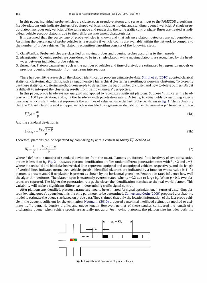
In this paper, probe headways are analyzed and applied to recognize significant platoons. Suppose h1 indicates the head-way with 100% penetration, and hp is the headway with penetration rate p. Actually, hp = Kh1 holds by assuming vehicleheadway as a constant, where K represents the number of vehicles since the last probe, as shown in Fig. 1. The probabilitythat the Kth vehicle is the next equipped vehicle is modeled by a geometric distribution with parameter p. The expectation is

EðhpÞ ¼h1

pð1aÞ

And the standard deviation is

StdðhpÞ ¼h1

ffiffiffiffiffiffiffiffiffiffiffiffi1� p

pp

ð1bÞ

Therefore, platoons can be separated by comparing hp with a critical headway Hp, defined as

Hp ¼h1

pþ k

h1

ffiffiffiffiffiffiffiffiffiffiffiffi1� p

pp

ð2Þ

where k defines the number of standard deviations from the mean. Platoons are formed if the headway of two consecutiveprobes is less than Hp. Fig. 2 illustrates platoon identification profiles under different penetration rates with h1 = 2 and k = 3,where the red solid and black dashed vertical lines represent equipped and unequipped vehicles, respectively, and the lengthof vertical lines indicates normalized vehicle speeds . Identified platoons are indicated by a function whose value is 1 if aplatoon is present and 0 if no platoon is present as shown by the horizontal green line. Penetration rates influence how wellthe algorithm performs. The platoon span is extremely overestimated when p = 0.2 due to large Hp. When p = 0.4, two pla-toons are captured. The higher the penetration rate p, the closer the identification matches to the real-world platoon. Thisvariability will make a significant difference in determining traffic signal control.

After platoons are identified, platoon parameters need to be estimated for signal optimization. In terms of a standing pla-toon (existing queue), queue length is the only parameter to be determined. Comert and Cetin (2009) proposed a probabilitymodel to estimate the queue size based on probe data. They claimed that only the location information of the last probe vehi-cle in the queue is sufficient for the estimation. Neumann (2010) proposed a maximal likelihood estimation method to esti-mate traffic demand, density profile, and queue length. However, neither of these studies considered the length of adischarging queue, when vehicle speeds are actually not zero. For moving platoons, the platoon size includes both the

1h

1Khhp =

Fig. 1. Illustration of headways of probe vehicles.

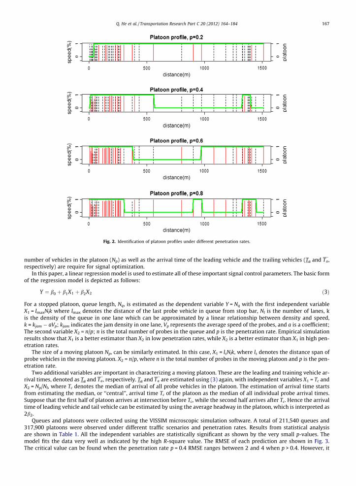
Fig. 2. Identification of platoon profiles under different penetration rates.

Q. He et al. / Transportation Research Part C 20 (2012) 164–184 167

number of vehicles in the platoon (Np) as well as the arrival time of the leading vehicle and the trailing vehicles (Ta and Ta,respectively) are require for signal optimization.

In this paper, a linear regression model is used to estimate all of these important signal control parameters. The basic formof the regression model is depicted as follows:

Y ¼ b0 þ b1X1 þ b2X2 ð3Þ

For a stopped platoon, queue length, Nq, is estimated as the dependent variable Y = Nq with the first independent variableX1 = lmaxNlk where lmax denotes the distance of the last probe vehicle in queue from stop bar, Nl is the number of lanes, kis the density of the queue in one lane which can be approximated by a linear relationship between density and speed,k = kjam � aVp; kjam indicates the jam density in one lane, Vp represents the average speed of the probes, and a is a coefficient;The second variable X2 = n/p; n is the total number of probes in the queue and p is the penetration rate. Empirical simulationresults show that X1 is a better estimator than X2 in low penetration rates, while X2 is a better estimator than X1 in high pen-etration rates.

The size of a moving platoon Np, can be similarly estimated. In this case, X1 = lsNlk, where ls denotes the distance span ofprobe vehicles in the moving platoon. X2 = n/p, where n is the total number of probes in the moving platoon and p is the pen-etration rate.

Two additional variables are important in characterizing a moving platoon. These are the leading and training vehicle ar-rival times, denoted as Ta and Ta, respectively. Ta and Ta are estimated using (3) again, with independent variables X1 = Tc andX2 = Np/Nl, where Tc denotes the median of arrival of all probe vehicles in the platoon. The estimation of arrival time startsfrom estimating the median, or ‘‘central’’, arrival time Tc of the platoon as the median of all individual probe arrival times.Suppose that the first half of platoon arrives at intersection before Tc, while the second half arrives after Tc. Hence the arrivaltime of leading vehicle and tail vehicle can be estimated by using the average headway in the platoon, which is interpreted as2b2.

Queues and platoons were collected using the VISSIM microscopic simulation software. A total of 211,540 queues and317,900 platoons were observed under different traffic scenarios and penetration rates. Results from statistical analysisare shown in Table 1. All the independent variables are statistically significant as shown by the very small p-values. Themodel fits the data very well as indicated by the high R-square value. The RMSE of each prediction are shown in Fig. 3.The critical value can be found when the penetration rate p = 0.4 RMSE ranges between 2 and 4 when p > 0.4. However, it

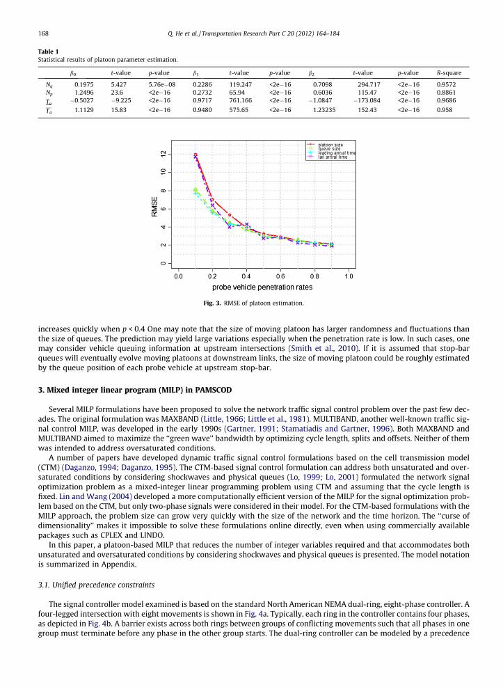
Table 1Statistical results of platoon parameter estimation.

b0 t-value p-value b1 t-value p-value b2 t-value p-value R-square

Nq 0.1975 5.427 5.76e�08 0.2286 119.247 <2e�16 0.7098 294.717 <2e�16 0.9572Np 1.2496 23.6 <2e�16 0.2732 65.94 <2e�16 0.6036 115.47 <2e�16 0.8861

Ta�0.5027 �9.225 <2e�16 0.9717 761.166 <2e�16 �1.0847 �173.084 <2e�16 0.9686

Ta 1.1129 15.83 <2e�16 0.9480 575.65 <2e�16 1.23235 152.43 <2e�16 0.958

Fig. 3. RMSE of platoon estimation.

168 Q. He et al. / Transportation Research Part C 20 (2012) 164–184

increases quickly when p < 0.4 One may note that the size of moving platoon has larger randomness and fluctuations thanthe size of queues. The prediction may yield large variations especially when the penetration rate is low. In such cases, onemay consider vehicle queuing information at upstream intersections (Smith et al., 2010). If it is assumed that stop-barqueues will eventually evolve moving platoons at downstream links, the size of moving platoon could be roughly estimatedby the queue position of each probe vehicle at upstream stop-bar.

3. Mixed integer linear program (MILP) in PAMSCOD

Several MILP formulations have been proposed to solve the network traffic signal control problem over the past few dec-ades. The original formulation was MAXBAND (Little, 1966; Little et al., 1981). MULTIBAND, another well-known traffic sig-nal control MILP, was developed in the early 1990s (Gartner, 1991; Stamatiadis and Gartner, 1996). Both MAXBAND andMULTIBAND aimed to maximize the ‘‘green wave’’ bandwidth by optimizing cycle length, splits and offsets. Neither of themwas intended to address oversaturated conditions.

A number of papers have developed dynamic traffic signal control formulations based on the cell transmission model(CTM) (Daganzo, 1994; Daganzo, 1995). The CTM-based signal control formulation can address both unsaturated and over-saturated conditions by considering shockwaves and physical queues (Lo, 1999; Lo, 2001) formulated the network signaloptimization problem as a mixed-integer linear programming problem using CTM and assuming that the cycle length isfixed. Lin and Wang (2004) developed a more computationally efficient version of the MILP for the signal optimization prob-lem based on the CTM, but only two-phase signals were considered in their model. For the CTM-based formulations with theMILP approach, the problem size can grow very quickly with the size of the network and the time horizon. The ‘‘curse ofdimensionality’’ makes it impossible to solve these formulations online directly, even when using commercially availablepackages such as CPLEX and LINDO.

In this paper, a platoon-based MILP that reduces the number of integer variables required and that accommodates bothunsaturated and oversaturated conditions by considering shockwaves and physical queues is presented. The model notationis summarized in Appendix.

3.1. Unified precedence constraints

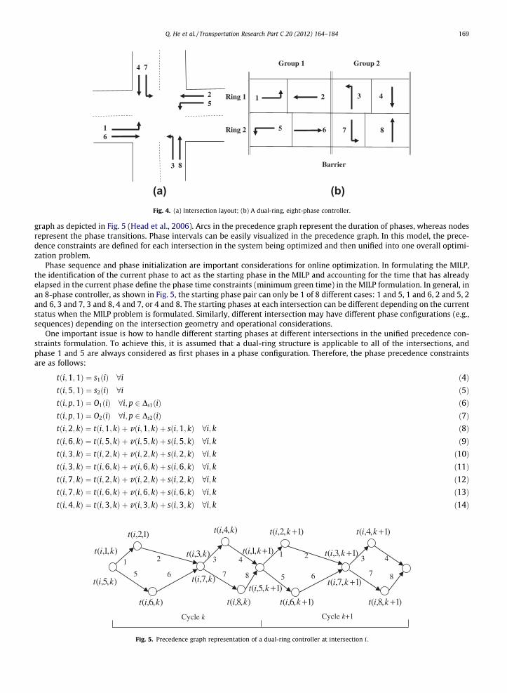
The signal controller model examined is based on the standard North American NEMA dual-ring, eight-phase controller. Afour-legged intersection with eight movements is shown in Fig. 4a. Typically, each ring in the controller contains four phases,as depicted in Fig. 4b. A barrier exists across both rings between groups of conflicting movements such that all phases in onegroup must terminate before any phase in the other group starts. The dual-ring controller can be modeled by a precedence

4 7

2 5

3 8

6 1

1 2 3 4

5 6 7 8

Ring 1

Ring 2

Group 1 Group 2

Barrier

(b)(a)Fig. 4. (a) Intersection layout; (b) A dual-ring, eight-phase controller.

Q. He et al. / Transportation Research Part C 20 (2012) 164–184 169

graph as depicted in Fig. 5 (Head et al., 2006). Arcs in the precedence graph represent the duration of phases, whereas nodesrepresent the phase transitions. Phase intervals can be easily visualized in the precedence graph. In this model, the prece-dence constraints are defined for each intersection in the system being optimized and then unified into one overall optimi-zation problem.

Phase sequence and phase initialization are important considerations for online optimization. In formulating the MILP,the identification of the current phase to act as the starting phase in the MILP and accounting for the time that has alreadyelapsed in the current phase define the phase time constraints (minimum green time) in the MILP formulation. In general, inan 8-phase controller, as shown in Fig. 5, the starting phase pair can only be 1 of 8 different cases: 1 and 5, 1 and 6, 2 and 5, 2and 6, 3 and 7, 3 and 8, 4 and 7, or 4 and 8. The starting phases at each intersection can be different depending on the currentstatus when the MILP problem is formulated. Similarly, different intersection may have different phase configurations (e.g.,sequences) depending on the intersection geometry and operational considerations.

One important issue is how to handle different starting phases at different intersections in the unified precedence con-straints formulation. To achieve this, it is assumed that a dual-ring structure is applicable to all of the intersections, andphase 1 and 5 are always considered as first phases in a phase configuration. Therefore, the phase precedence constraintsare as follows:

tði;1;1Þ ¼ s1ðiÞ 8i ð4Þtði;5;1Þ ¼ s2ðiÞ 8i ð5Þtði; p;1Þ ¼ O1ðiÞ 8i;p 2 Ds1ðiÞ ð6Þtði; p;1Þ ¼ O2ðiÞ 8i;p 2 Ds2ðiÞ ð7Þtði;2; kÞ ¼ tði;1; kÞ þ vði;1; kÞ þ sði;1; kÞ 8i; k ð8Þtði;6; kÞ ¼ tði;5; kÞ þ vði;5; kÞ þ sði;5; kÞ 8i; k ð9Þtði;3; kÞ ¼ tði;2; kÞ þ vði;2; kÞ þ sði;2; kÞ 8i; k ð10Þtði;3; kÞ ¼ tði;6; kÞ þ vði;6; kÞ þ sði;6; kÞ 8i; k ð11Þtði;7; kÞ ¼ tði;2; kÞ þ vði;2; kÞ þ sði;2; kÞ 8i; k ð12Þtði;7; kÞ ¼ tði;6; kÞ þ vði;6; kÞ þ sði;6; kÞ 8i; k ð13Þtði;4; kÞ ¼ tði;3; kÞ þ vði;3; kÞ þ sði;3; kÞ 8i; k ð14Þ

1

5

2

6

1

5

2

6

3

7

4

8

3

7

4

8

Cycle k Cycle k+1

),5,( kit

)1,2,(it

),6,( kit

),3,( kit

),7,( kit

),4,( kit

),8,( kit

)1,2,( +kit

)1,6,( +kit

)1,1,( +kit

)1,5,( +kit

)1,4,( +kit

)1,8,( +kit

)1,3,( +kit

)1,7,( +kit

),1,( kit

Fig. 5. Precedence graph representation of a dual-ring controller at intersection i.

170 Q. He et al. / Transportation Research Part C 20 (2012) 164–184

tði;8; kÞ ¼ tði;7; kÞ þ vði;7; kÞ þ sði;7; kÞ 8i; k ð15Þtði;1; kþ 1Þ ¼ tði;4; kÞ þ vði;4; kÞ 8i; k ð16Þtði;1; kþ 1Þ ¼ tði;8; kÞ þ vði;8; kÞ 8i; k ð17Þtði;5; kþ 1Þ ¼ tði;4; kÞ þ vði;4; kÞ 8i; k ð18Þtði;5; kþ 1Þ ¼ tði;8; kÞ þ vði;8; kÞ 8i; k ð19Þvði; p; kÞ ¼ gði; p; kÞ þ Yði; pÞ þ Rði;pÞ 8i; p R DnonðiÞ [ DpðiÞ; k ð20Þvði; p; kÞ ¼ 0 8i;p 2 DnonðiÞ [ DpðiÞ; k ð21Þgði;p; kÞ ¼ 0 8i; p 2 DnonðiÞ [ DpðiÞ; k ð22Þsði; p; kÞ ¼ 0 8i;p; k P 2 or 8i;p R Ds1ðiÞ [ Ds2ðiÞ [ DpðiÞ; k ¼ 1 ð23ÞX

p

Xk

sði;p; kÞ 6 Z 8i;p; k ð24Þ

Gminði;pÞ 6 gði;p; kÞ 6 Gminði;pÞ 8i;p R Ds1ðiÞ [ Ds2ðiÞ [ DpðiÞ [ DnonðiÞ; k ð25Þgði;p; kÞP Gminði;pÞ � Eði;pÞ 8i;p 2 Ds1ðiÞ [ Ds2ðiÞ; k ð26Þ

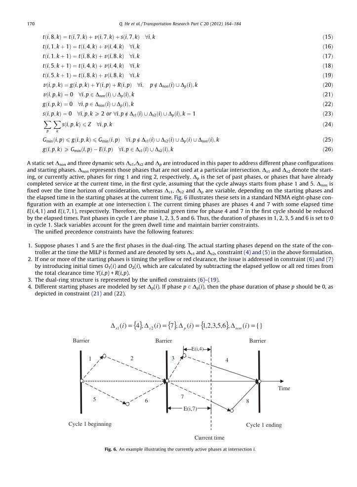
A static set Dnon and three dynamic sets Ds1,Ds2 and Dp are introduced in this paper to address different phase configurationsand starting phases. Dnon represents those phases that are not used at a particular intersection. Ds1 and Ds2 denote the start-ing, or currently active, phases for ring 1 and ring 2, respectively. Dp is the set of past phases, or phases that have alreadycompleted service at the current time, in the first cycle, assuming that the cycle always starts from phase 1 and 5. Dnon isfixed over the time horizon of consideration, whereas Ds1, Ds2 and Dp are variable, depending on the starting phases andthe elapsed time in the starting phases at the current time. Fig. 6 illustrates these sets in a standard NEMA eight-phase con-figuration with an example at one intersection i. The current timing phases are phases 4 and 7 with some elapsed timeE(i,4,1) and E(i,7,1), respectively. Therefore, the minimal green time for phase 4 and 7 in the first cycle should be reducedby the elapsed times. Past phases in cycle 1 are phase 1, 2, 3, 5 and 6. Thus, the duration of phases in 1, 2, 3, 5 and 6 is set to 0in cycle 1. Slack variables account for the green dwell time and maintain barrier constraints.

The unified precedence constraints have the following features:

1. Suppose phases 1 and 5 are the first phases in the dual-ring. The actual starting phases depend on the state of the con-troller at the time the MILP is formed and are denoted by sets Ds1 and Ds2, constraint (4) and (5) in the above formulation.

2. If one or more of the starting phases is timing the yellow or red clearance, the issue is addressed in constraint (6) and (7)by introducing initial times O1(i) and O2(i), which are calculated by subtracting the elapsed yellow or all red times fromthe total clearance time Y(i,p) + R(i,p).

3. The dual-ring structure is represented by the unified constraints (6)–(19).4. Different starting phases are modeled by set Dp(i). If phase p 2Dp(i), then the phase duration of phase p should be 0, as

depicted in constraint (21) and (22).

Cycle 1 beginning

Barrier

Cycle 1 ending

1 2

5 6

3 4

7 8

E(i,4)

E(i,7)

Time

Current time

{ } { } { } {})(,6,5,3,2,1)(,7)(,4)( 21 =Δ=Δ=Δ=Δ iiii nonpss

Barrier Barrier

Fig. 6. An example illustrating the currently active phases at intersection i.

Q. He et al. / Transportation Research Part C 20 (2012) 164–184 171

5. Slack variables are introduced only for green rest to fulfill the barrier constraints in the first cycle. This means the max-imal green constraints could be violated if the first barrier constraints must be satisfied. Constraint (23) and (24) ensurethat the slack variables are equal to zero in all of the phases after the starting phases. Green rest occurs when one ringreaches a barrier, or maximal green, but the other ring does not reach the barrier such that the ring will rest on the barrierto satisfy the barrier constraint, regardless of the maximal green time constraint.

6. The minimal green times of the starting phases can be less than the pre-defined minimum green time, Gmin(i,p), as thestarting phases have already been timing for e(i,p).

3.2. Platoon delay categorization and evaluation

Delay is perhaps the most commonly reported performance index in the literature of traffic signal control. Within thePAMSCOD formulation, before delay can be assessed, it is necessary to determine which cycle is selected to serve platoon(m, i,p, j), thereby determining the correct phase starting time, t(i,p,k), to calculate the delay of platoon (m, i,p, j).

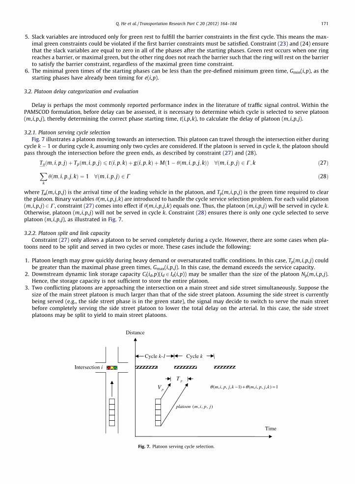
3.2.1. Platoon serving cycle selectionFig. 7 illustrates a platoon moving towards an intersection. This platoon can travel through the intersection either during

cycle k � 1 or during cycle k, assuming only two cycles are considered. If the platoon is served in cycle k, the platoon shouldpass through the intersection before the green ends, as described by constraint (27) and (28).

Taðm; i;p; jÞ þ Tpðm; i;p; jÞ 6 tði;p; kÞ þ gði; p; kÞ þMð1� hðm; i;p; j; kÞÞ 8ðm; i;p; jÞ 2 C; k ð27Þ

X

k

hðm; i; p; j; kÞ ¼ 1 8ðm; i;p; jÞ 2 C ð28Þ

where Ta(m, i,p, j) is the arrival time of the leading vehicle in the platoon, and Tp(m, i,p, j) is the green time required to clearthe platoon. Binary variables h(m, i,p, j,k) are introduced to handle the cycle service selection problem. For each valid platoon(m, i,p, j) 2 C, constraint (27) comes into effect if h(m, i,p, j,k) equals one. Thus, the platoon (m, i,p, j) will be served in cycle k.Otherwise, platoon (m, i,p, j) will not be served in cycle k. Constraint (28) ensures there is only one cycle selected to serveplatoon (m, i,p, j), as illustrated in Fig. 7.

3.2.2. Platoon split and link capacityConstraint (27) only allows a platoon to be served completely during a cycle. However, there are some cases when pla-

toons need to be split and served in two cycles or more. These cases include the following:

1. Platoon length may grow quickly during heavy demand or oversaturated traffic conditions. In this case, Tp(m, i,p, j) couldbe greater than the maximal phase green times, Gmax(i,p, j). In this case, the demand exceeds the service capacity.

2. Downstream dynamic link storage capacity Cl(id,p)(id 2 Id(i,p)) may be smaller than the size of the platoon Np(m, i,p, j).Hence, the storage capacity is not sufficient to store the entire platoon.

3. Two conflicting platoons are approaching the intersection on a main street and side street simultaneously. Suppose thesize of the main street platoon is much larger than that of the side street platoon. Assuming the side street is currentlybeing served (e.g., the side street phase is in the green state), the signal may decide to switch to serve the main streetbefore completely serving the side street platoon to lower the total delay on the arterial. In this case, the side streetplatoons may be split to yield to main street platoons.

Distance

Time

pV 1),,,,()1,,,,( =+− kjpimkjpim θθ

Cycle k-1 Cycle k

pT

),,,( jpimplatoon

Intersection i

Fig. 7. Platoon serving cycle selection.

172 Q. He et al. / Transportation Research Part C 20 (2012) 164–184

Platoon splitting in the first two cases is due to capacity constraints that cannot be violated. Platoon splitting in the thirdcase is due to the performance benefit of platoon splitting, which increases arterial progression. The details of arterial pro-gression will be discussed in the next section.

A positive variable ct(m, i,p, j) 2 [0,1] is introduced to ‘‘cut’’ the platoons into two cycles, assuming that platoon can beserved in no more than two cycles. Therefore, constraint (27) is rewritten as

Taðm; i;p; jÞ þ Tpðm; i;p; jÞ�ctðm; i;p; jÞ 6 tði;p; kÞ þ gði;p; kÞ þMð1� hðm; i;p; j; kÞÞ 8ðm; i; p; jÞ 2 C; k ð29Þ

The first part of platoon (m, i,p, j) is served in cycle k, whereas the remaining is assigned to be served in cycle k + 1. Theremaining Np(m, i,p, j)⁄(1 � ct(m, i,p, j)) vehicles are delayed by at least one cycle. Assuming a platoon can be served in, atmost, two cycles, a delay penalty, dpen(m, i,p, j), is added into the formulation to account for the delay as follows:

dpenðm; i;p; jÞ ¼ Npðm; i;p; jÞ�ð1� ctðm; i; p; jÞÞ�Cr 8ðm; i;p; jÞ 2 C ð30Þ

where Cr is the reference cycle length, which represents an empirical estimation of cycle length, such as average over thehistorical cycles.

If one platoon is cut in the past cycle, the remaining vehicles in the platoon become the first queue at the stop bar. Thismeans that the remaining vehicles in the platoon will be served in the next cycle without any queue delay. If the remainingplatoon has to be further cut in the next cycle, the new delay penalty will be considered in the formulation by solving an-other MILP based on a rolling horizon optimization approach. Therefore, constraint (30) can be used to roughly estimate howmuch delay will be generated for platoon splits.

Green times are subject to the required time to clear the platoon in the selected cycle. Thus, additional lower bounds ofg(i,p,k) are added in the formulation as constraint (31):

gði;p; kÞP Tpðm; i;p; jÞ�ctðm; i; p; jÞ �Mð1� hðm; i;p; j; kÞÞ 8ðm; i;p; jÞ 2 C ð31Þ

Queue spillback occurs during oversaturated conditions, which can cause de facto red (Abu-Lebdeh and Benekohal, 1997). Defacto red is an extreme case of queue build-up that is due to the complete blockage of upstream signals when no traffic candischarge during a green phase. To avoid de facto red and assign green times efficiently, the link storage capacity is utilized toset an upper limit on the split ratio in constraint (32):

ctðm; i; p; jÞ 6 Clðid; pÞ=Npðm; i;p; jÞ 8ðm; i;p; jÞ 2 C ð32Þ

The experiments described in Section 4 used microscopic simulations to demonstrate the significance of constraint (32) dur-ing oversaturated conditions. The network throughput was increased by 10 � 20%, and overall delay was decreased by5 � 10% by considering platoon split and link capacity for the oversaturated arterial.

3.2.3. Delay evaluationTo evaluate the total delay of a platoon, delay is divided into two categories: signal delay and queue delay. These two

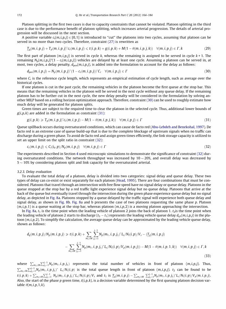
types of delay can co-exist or exist separately for each platoon (Head, 1995). There are four combinations that must be con-sidered. Platoons that travel through an intersection with free flow speed have no signal delay or queue delay. Platoons in thequeue stopped at the stop bar by a red traffic light experience signal delay but no queue delay. Platoons that arrive at theback of the queue but eventually travel through the intersection during the green phase experience queue delay but no signaldelay, as depicted in Fig. 8a. Platoons stopped by a queue delayed by the traffic signal will experience both queue delay andsignal delay, as shown in Fig. 8b. Fig. 8a and b presents the case of two platoons requesting the same phase p. Platoon(m, i,p,1) is a queue waiting at the stop bar, whereas platoon (m, i,p,2) is a moving platoon approaching the intersection.

In Fig. 8a, t1 is the time point when the leading vehicle of platoon 2 joins the back of platoon 1. t2is the time point whenthe leading vehicle of platoon 2 starts to discharge (t2 � t1) represents the leading vehicle queue delay dq1(m, i,p, j) in the pla-toon (m, i,p,2). To simplify the calculation, the average queue delay can be approximated by the leading vehicle queue delay,shown as follows:

dqðm; i;p; jÞ=Npðm; i; p; jÞP tði;p; kÞ þX

m12M

Xj�1

j1¼1

Npðm1; i;p; j1Þ�Ls=Nlði;pÞ=Vs � ðTaðm; i; p; jÞ

�X

m12M

Xj�1

j1¼1

Npðm1; i; p; j1Þ�Ls=Nlði;pÞ=Vpðm; i;p; jÞÞ �Mð1� hðm; i;p;1; kÞÞ 8ðm; i; p; jÞ 2 C; k

ð33Þ

whereP

m12M

Pj�1j1¼1Npðm1; i; p; j1Þ represents the total number of vehicles in front of platoon (m, i,p, j). Thus,P

m12M

Pj�1j1¼1Npðm1; i; p; j1Þ

� Ls=Nlði; pÞ is the total queue length in front of platoon (m, i,p, j). t2 can be found to be

tði; p; kÞ þP

m12M

Pj�1j1¼1 Npðm1; i; p; j1Þ

�Ls=Nlði; pÞ=Vs and t1 is Taðm; i; p; jÞ �P

m12M

Pj�1j1¼1Npðm1; i; p; j1Þ

�Ls=Nlði; pÞ=Vpðm; i; p; jÞ.Also, the start of the phase p green time, t(i,p,k), is a decision variable determined by the first queuing platoon decision var-iable h(m, i,p,1,k).

Distance

Time

),,( kpit

)1,,,( pimsv

fv

)2,,,(1 pimdq

)2,,,(1 pimds

)1,,( +kpit

)2,,,( pim

pv

(b) 1)1,2,,,(

1),1,,,(

=+=

kpim

kpim

θθ

Intersection i

Distance

Time

),,( kpit

)1,,,( pim

sv

fv

)2,,,(1 pimdq)1,,( +kpit

)2,,,( pimpv

1),2,,,(

1),1,,,(

==

kpim

kpim

θθ

(a)

Intersection i

1t 2t

Fig. 8. (a) Queue delay when two platoons are served in the same cycle; (b) Queue delay and signal delay when two platoons are served in different cycles.

Q. He et al. / Transportation Research Part C 20 (2012) 164–184 173

The queue delay can affect the arrival of a platoon; hence, constraint (29) holds only if the queue delay is equal to zero.Otherwise, queue delay should be included in constraint (29) to estimate the realized arrival time of the platoon at the stopbar, as described by constraint (34):

Taðm; i;p; jÞ þ dqðm; i;p; jÞ=Npðm; i;p; jÞ þ Tpðm; i;p; jÞctðm; i;p; jÞ6 tði; p; kÞ þ gði;p; kÞ þMð1� hðm; i; p; j; kÞÞ 8ðm; i;p; jÞ 2 C; k ð34Þ

Signal delay is generated by stopping the moving platoon due to a red phase rather than the leading platoon. An example ofsignal delay is illustrated in Fig. 8b. The platoon (m, i,p,2) is stopped by the discharging queue and then arrives during the redphase. The leading vehicle signal delay can be determined based on the starting time of phase p in cycle k + 1, t(i,p,k + 1).

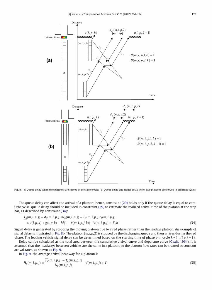
Delay can be calculated as the total area between the cumulative arrival curve and departure curve (Gazis, 1964). It isassumed that the headways between vehicles are the same in a platoon, so the platoon flow rates can be treated as constantarrival rates, as shown as Fig. 9.

In Fig. 9, the average arrival headway for a platoon is

Hpðm; i; p; jÞ ¼Taðm; i;p; jÞ � Taðm; i;p; jÞ

Npðm; i;p; jÞ8ðm; i; p; jÞ 2 C ð35Þ

),,,( jpimN p

Cum. Veh.

Hp Hs

),,,( jpimTa ),,( kpit Time

),,,( jpimds

Fig. 9. Signal delay evaluation for the leading platoon.

174 Q. He et al. / Transportation Research Part C 20 (2012) 164–184

where Taðm; i; p; jÞ � Taðm; i; p; jÞ represents the arrival time difference between the leading vehicle and trailing vehicle in theplatoon. If it is a queuing platoon, Eq. (35) holds as

Taðm; i;p; jÞ ¼ Taðm; i; p; jÞ ¼ 0 ð36Þ

which makes Hp = 0 for queuing platoons.The headway for saturation departure can be calculated as

Hsði;pÞ ¼Hs1

Nlði;pÞ8i;p ð37Þ

where Hs is the average headway of all the departure vehicles across all the output lanes, Hs1 is saturation flow headway in asingle lane (usually 2 s), and Nl(i,p) is number of lanes being served by phase p at intersection i. The signal delay of the lead-ing platoon is the summation of the vehicle delays measured between the arrival curve and departure curve illustrated inFig. 9. In terms of non-leading platoons, the service time of platoon (m, i,p, j) will be delayed. It is necessary to account forthe green time used to serve the preceding platoons, which is

Pj�1j1¼1 ½hðm; i; p; j1; kÞ

�Tpðm; i; p; j1Þ�, shown in constraint (38).

dsðm; i;p; jÞPXNpðm;i;p;jÞ

n¼1

tði;p; kÞ þX

m12M

Xj�1

j1¼1

½hðm1; i;p; j1; kÞ�Tpðm1; i; p; j1Þ� þ ðn� 1ÞHsðm; i; p; jÞ

(

�½Taðm; i; p; jÞÞ þ ðn� 1ÞHpði; pÞ�)�Mð1� hðm; i; p; j; kÞÞ 8j; ðm; i;p; jÞ 2 C; k ð38Þ

3.3. Multi-modal dynamical progression

The state of practice of traffic signal control strategies is coordinated-actuated signal control. Coordinated-actuatedsignals can offer additional flexibility compared with fixed-time traffic signals because of their ability to respond to cycle-by-cycle variation in traffic demand while still being able to provide progression for arterial movement. Traditionally, arterialcoordination is managed through the determination of appropriate offsets, splits, and a common cycle length at each inter-section. The ‘‘optimal’’ parameters of coordination signal plan can obtained by off-line signal optimization software, such asTRANSYT (Wallace et al., 1998), SYNCHRO (Trafficware, 2009) and PASSER (Chaudhary and Chu, 2003). However, the trafficflows optimized in signal optimization software are considered to be deterministic. In actuality, real-time traffic flow, eventime-of-day traffic flow, can vary significantly (Yin, 2008). Previous on-line traffic-responsive (adaptive) signal control sys-tems (Hunt, 1982; Luk, 1984) are able to adjust the coordination parameters (cycle length, offsets and splits) to fit the cur-rent detected traffic data, but the optimized plan assumes a constraint that every intersection must have the same cyclelength, which may not be the best solution for every intersection on the arterial based on real-time traffic data. It is not nec-essary to maintain the concept of a common cycle length or an offset that is constant during each cycle, as it is assumed thatmulti-modal traffic data are available through vehicle-to-infrastructure communications.

A platoon-based dynamic coordination strategy is proposed as part of PAMSCOD to consider not only the current inter-section but also the progression through downstream intersections given the path information of each vehicle. The conceptis to consider platoon queue delay and signal delay in the current intersection as well as its potential queue delay and signaldelay at the next downstream intersection. Another binary variable h0(m, i,p, j,c) is introduced into the PAMSCOD formulation

Q. He et al. / Transportation Research Part C 20 (2012) 164–184 175

to perform cycle selection at downstream intersection, id 2 Id(i,p), for platoon (m, i,p, j) approaching the current intersection ifor phase p. Again, it is assumed that only two cycles will be considered to serve a platoon. The platoon service cycle selectionconstraints are shown below:

tði; p; kÞ þX

m12M

Xj�1

j1¼1

½hðm1; i;p; j1; kÞ�Tpðm1; i;p; j1Þ� þ F�dTpðm; i;p; jÞ�ctðm; i;p; jÞ þ Ttði; idÞ þ Tst þ d0qðm; i; p; jÞ=Npðm; i;p; jÞ

6 tðid;p; cÞ þ gðid; p; cÞ þMð2� hðm; i;p; j; kÞ � h0ðm; i; p; j; cÞÞ 8ðm; i;p; jÞ 2 Ce [ Cw; k; c ð39Þ

Xc

h0ðm; i;p; j; cÞ ¼ 1 8ðm; i;p; jÞ 2 Ce [ Cw ð40Þ

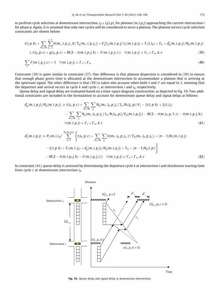
Constraint (39) is quite similar to constraint (27). One difference is that platoon dispersion is considered in (39) to ensurethat enough phase green time is allocated at the downstream intersection to accommodate a platoon that is arriving atthe upstream signal. The other difference is that (39) is taken into account when both h and h0 are equal to 1, meaning thatthe departure and arrival occurs in cycle k and cycle c, at intersection i and id, respectively.

Queue delay and signal delay are evaluated based on a time–space diagram construction, as depicted in Fig. 10. Two addi-tional constraints are included in the formulation to account for downstream queue delay and signal delay as follows:

d0qðm; i;p; jÞ=Npðm; i;p; jÞP tðid;p; cÞ þX

m12M

Xj1

Npðm1; id;p; j1Þ�Ls=Nlðid;pÞ=Vs � ftði;p; kÞ þ ½Lði; idÞ

�X

m12M

Xj1

Npðm1; id;p; j1Þ�Ls=Nlðid; pÞ�=Vpðm; i;p; jÞg �Mð2� hðm; id;p;1; cÞ � hðm; i;p; j; kÞÞ

8ðm; i; p; jÞ 2 Ce [ Cw; k; c ð41Þ

d0sðm; i;p; jÞP Prðm; i; idÞ�XNpðm;i;p;jÞ

n¼1

tðid;p; cÞ þX

m12M

Xj1

½hðm1; id;p; j1; cÞ�Tpðm1; id;p; j1Þ� þ ðn� 1ÞHsðm; i;p; jÞ

(

� ½tði; p; kÞ þ Ttðm; i; idÞ þ d0qðm; i;p; jÞ=Npðm; i;p; jÞ þ Tst þ ðn� 1ÞHpði;pÞ�)

�Mð2� hðm; i;p; j; kÞ � h0ðm; i;p; j; cÞÞ 8ðm; i;p; jÞ 2 Ce [ Cw; k; c ð42Þ

In constraint (41), queue delay is assessed by determining the departure cycle k at intersection i and shockwave starting timefrom cycle c at downstream intersection id.

Distance

Time

Intersection id

Intersection i

diiLL ,

),,( cpit d

),,( kpit

sv

fv

qd 'sd '

)1,,( +cpit d

)1,,( +kpit

Fig. 10. Queue delay and signal delay at downstream intersection.

176 Q. He et al. / Transportation Research Part C 20 (2012) 164–184

The platoon departure cycle is controlled by binary variable h(m, i,p, j,k), whereas the shockwave starting time iscontrolled by binary variable h(m, id,p,1,c), denoting that the first platoon to arrive at the downstream intersection is servedin cycle c.

In constraint (42), signal delay is addressed by choosing the departure cycle k at intersection i and then the departurecycle c at downstream intersection id, controlled by binary variables h(m, i,p, j,k) and h0(m, id,p, j,c), respectively.Pr(m, i, id) 2 [0,1] represents the percentage of the vehicles remaining in the platoon after traveling through link (i, id).

3.4. Objective and summary of PAMSCOD

Usually, the objective of traffic signal control algorithms is to minimize a disutility function, such as travel time, delay ornumber of stops, or maximize a utility function, such as network throughput. The proposed formulation aims to serve all ofthe platoons in jKj cycles using a rolling horizon approach. Hence, the throughput cannot be evaluated in the formulation.The number of stops is not computable due to the lack of an exact traffic flow model in the formulation. However, the totaldelay can be approximately assessed by the constraints derived in the previous sections.

The objective function will be to minimize the total weighted delay as well as the sum of slack variables representing thetotal green rest time, as described by Eq. (43). The delay weight factor W(m, i,p, j) can be set to different values for each modeas well as each different platoon. Weight factors can depend on the priority level of the mode and can be adjusted for indi-vidual vehicles according to other real-time information, such as vehicle occupancy. It is assumed that emergency vehicleswill receive a very high level of priority and can be considered in a complementary and separate formulation.

A summary of the formulation is depicted as follows:

Objective : MinimizeX

ðm;i;p;jÞ2CWðm; i; p; jÞ� dsðm; i; p; jÞ þ dqðm; i; p; jÞ þ dpenðm; i;p; jÞ þ d0sðm; i;p; jÞ þ d0qðm; i;p; jÞ

h i

þ aXði;p;kÞ

sði;p; kÞ ð43Þ

Subject toPrecedence constraints: (4)–(26)Selection constraints at current intersections: (28), (31), and (34)Delay evaluation at current intersections: (30), (33), and (38)Link capacity constraints: (32)Selection constraints at downstream intersections: (39) and (40)Delay evaluation at downstream intersections: (41) and (42)

Variables h and h0 are binary decision variables, and all other variables are non-negative.

The maximal number of integer variables in PAMSCOD is equal to 2jCkKj, where 2 indicates two sets of integer variables:h and h0,jCj the number of existing platoons, and jKj the number of considered cycles. The solution times of this formulationvary depending on the size of the network and the traffic saturation condition. Rather, solution times are directly influencedby the total number of platoons, the size of platoons and number of cycles considered. Therefore, only a couple of the mostsignificant platoons are considered in each phase. Moreover, a rolling horizon is adopted to solve MILP every 30 s for 4 cyclesin the future.

The formulation was tested with GAMS/CPLEX 10.1 on a PC with a dual core 2.67-GHz processor and 3.5 Gb of memory.The test network is the same as that described in Section 4, shown in Fig. 11. For uncongested traffic conditions with noresidual queue, the solution times are less than 1 s in most cases, as shown in Table 2. However, for congested and oversat-urated conditions, the solution times extend from a few seconds up to a couple of minutes to achieve an optimality gap near10%. The solution times have a significant impact on the implementation of an algorithm such as PAMSCOD in the field. Thus,the authors are actively developing simplified formulations and heuristic algorithms for future real-time applications.

1 2 3 4 5 6 7 8

yawnonrevlAdRbulCyrtnuoCevAllebpmaCevAdilcuE

Route 4EB

Route 6NB

Route 6SB Route 15SB Route 17SB

Route 15NB Route 17NB

Route 4WB

Route 11NB

Route 11SB

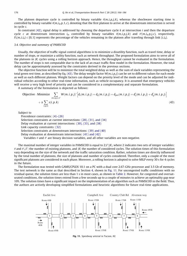
Fig. 11. Speedway arterial in Tucson, AZ.

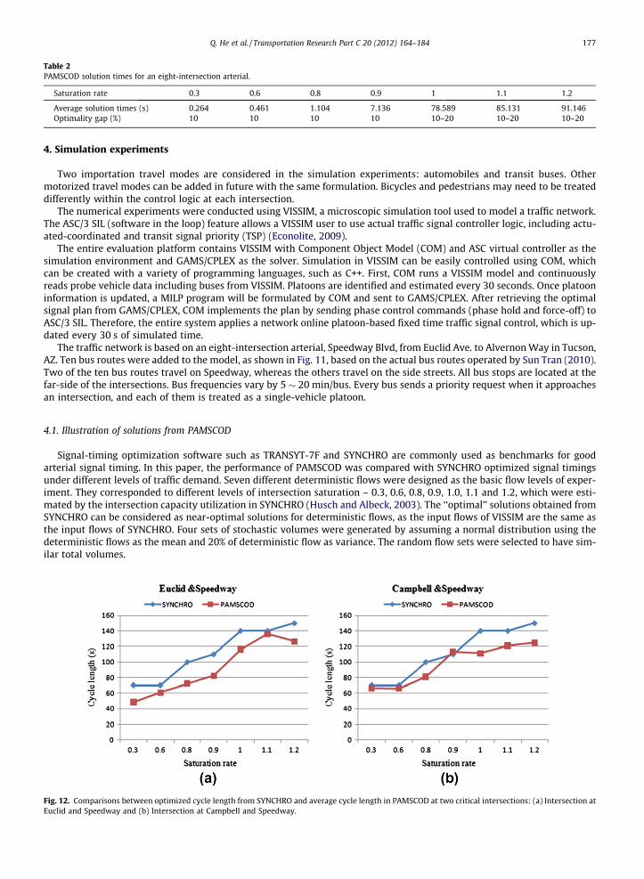
Table 2PAMSCOD solution times for an eight-intersection arterial.

Saturation rate 0.3 0.6 0.8 0.9 1 1.1 1.2

Average solution times (s) 0.264 0.461 1.104 7.136 78.589 85.131 91.146Optimality gap (%) 10 10 10 10 10–20 10–20 10–20

Q. He et al. / Transportation Research Part C 20 (2012) 164–184 177

4. Simulation experiments

Two importation travel modes are considered in the simulation experiments: automobiles and transit buses. Othermotorized travel modes can be added in future with the same formulation. Bicycles and pedestrians may need to be treateddifferently within the control logic at each intersection.

The numerical experiments were conducted using VISSIM, a microscopic simulation tool used to model a traffic network.The ASC/3 SIL (software in the loop) feature allows a VISSIM user to use actual traffic signal controller logic, including actu-ated-coordinated and transit signal priority (TSP) (Econolite, 2009).

The entire evaluation platform contains VISSIM with Component Object Model (COM) and ASC virtual controller as thesimulation environment and GAMS/CPLEX as the solver. Simulation in VISSIM can be easily controlled using COM, whichcan be created with a variety of programming languages, such as C++. First, COM runs a VISSIM model and continuouslyreads probe vehicle data including buses from VISSIM. Platoons are identified and estimated every 30 seconds. Once platooninformation is updated, a MILP program will be formulated by COM and sent to GAMS/CPLEX. After retrieving the optimalsignal plan from GAMS/CPLEX, COM implements the plan by sending phase control commands (phase hold and force-off) toASC/3 SIL. Therefore, the entire system applies a network online platoon-based fixed time traffic signal control, which is up-dated every 30 s of simulated time.

The traffic network is based on an eight-intersection arterial, Speedway Blvd, from Euclid Ave. to Alvernon Way in Tucson,AZ. Ten bus routes were added to the model, as shown in Fig. 11, based on the actual bus routes operated by Sun Tran (2010).Two of the ten bus routes travel on Speedway, whereas the others travel on the side streets. All bus stops are located at thefar-side of the intersections. Bus frequencies vary by 5 � 20 min/bus. Every bus sends a priority request when it approachesan intersection, and each of them is treated as a single-vehicle platoon.

4.1. Illustration of solutions from PAMSCOD

Signal-timing optimization software such as TRANSYT-7F and SYNCHRO are commonly used as benchmarks for goodarterial signal timing. In this paper, the performance of PAMSCOD was compared with SYNCHRO optimized signal timingsunder different levels of traffic demand. Seven different deterministic flows were designed as the basic flow levels of exper-iment. They corresponded to different levels of intersection saturation – 0.3, 0.6, 0.8, 0.9, 1.0, 1.1 and 1.2, which were esti-mated by the intersection capacity utilization in SYNCHRO (Husch and Albeck, 2003). The ‘‘optimal’’ solutions obtained fromSYNCHRO can be considered as near-optimal solutions for deterministic flows, as the input flows of VISSIM are the same asthe input flows of SYNCHRO. Four sets of stochastic volumes were generated by assuming a normal distribution using thedeterministic flows as the mean and 20% of deterministic flow as variance. The random flow sets were selected to have sim-ilar total volumes.

Fig. 12. Comparisons between optimized cycle length from SYNCHRO and average cycle length in PAMSCOD at two critical intersections: (a) Intersection atEuclid and Speedway and (b) Intersection at Campbell and Speedway.

178 Q. He et al. / Transportation Research Part C 20 (2012) 164–184

First, the output cycle lengths of PAMSCOD were compared with SYNCHRO’s optimal cycle length. Average cycle lengthswith seven volume levels were recorded at the two most saturated intersections: Euclid and Speedway, and Campbell andSpeedway. Fig. 12a and b plot the curves of cycle length with PAMSCOD and SYNCHRO at these two intersections, respec-tively. The results show that PAMSCOD’s cycle lengths are slightly shorter than SYNCHRO’s optimized cycle lengths, butPAMSCOD’s cycle lengths follow the tendency that arterial cycle length is proportional to flow levels. Previous studies show

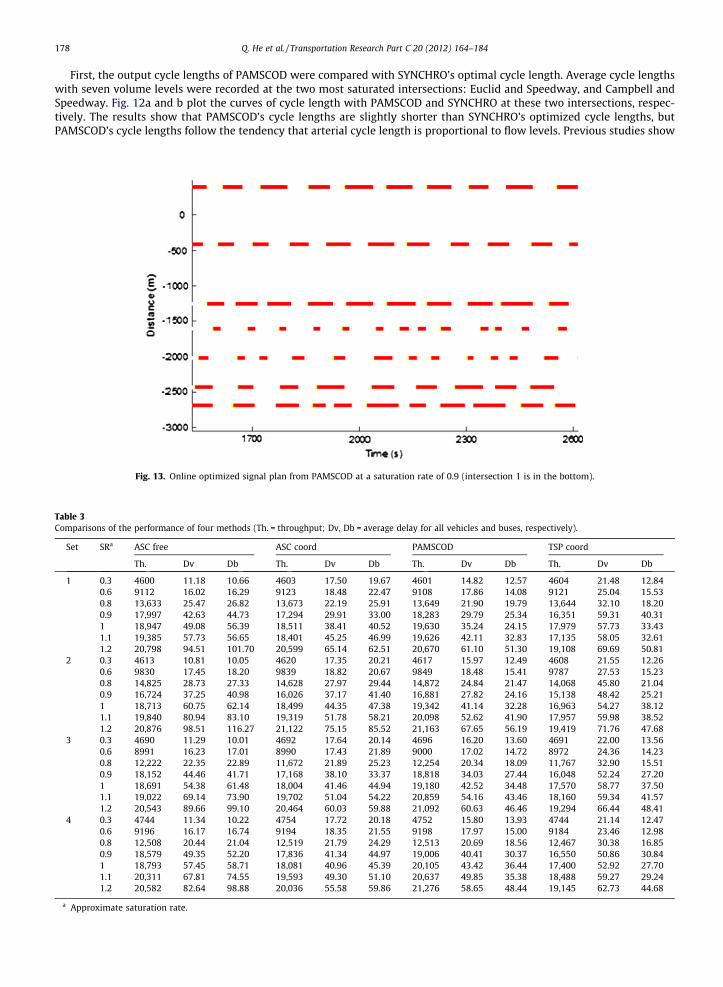
Fig. 13. Online optimized signal plan from PAMSCOD at a saturation rate of 0.9 (intersection 1 is in the bottom).

Table 3Comparisons of the performance of four methods (Th. = throughput; Dv, Db = average delay for all vehicles and buses, respectively).

Set SRa ASC free ASC coord PAMSCOD TSP coord

Th. Dv Db Th. Dv Db Th. Dv Db Th. Dv Db

1 0.3 4600 11.18 10.66 4603 17.50 19.67 4601 14.82 12.57 4604 21.48 12.840.6 9112 16.02 16.29 9123 18.48 22.47 9108 17.86 14.08 9121 25.04 15.530.8 13,633 25.47 26.82 13,673 22.19 25.91 13,649 21.90 19.79 13,644 32.10 18.200.9 17,997 42.63 44.73 17,294 29.91 33.00 18,283 29.79 25.34 16,351 59.31 40.311 18,947 49.08 56.39 18,511 38.41 40.52 19,630 35.24 24.15 17,979 57.73 33.431.1 19,385 57.73 56.65 18,401 45.25 46.99 19,626 42.11 32.83 17,135 58.05 32.611.2 20,798 94.51 101.70 20,599 65.14 62.51 20,670 61.10 51.30 19,108 69.69 50.81

2 0.3 4613 10.81 10.05 4620 17.35 20.21 4617 15.97 12.49 4608 21.55 12.260.6 9830 17.45 18.20 9839 18.82 20.67 9849 18.48 15.41 9787 27.53 15.230.8 14,825 28.73 27.33 14,628 27.97 29.44 14,872 24.84 21.47 14,068 45.80 21.040.9 16,724 37.25 40.98 16,026 37.17 41.40 16,881 27.82 24.16 15,138 48.42 25.211 18,713 60.75 62.14 18,499 44.35 47.38 19,342 41.14 32.28 16,963 54.27 38.121.1 19,840 80.94 83.10 19,319 51.78 58.21 20,098 52.62 41.90 17,957 59.98 38.521.2 20,876 98.51 116.27 21,122 75.15 85.52 21,163 67.65 56.19 19,419 71.76 47.68

3 0.3 4690 11.29 10.01 4692 17.64 20.14 4696 16.20 13.60 4691 22.00 13.560.6 8991 16.23 17.01 8990 17.43 21.89 9000 17.02 14.72 8972 24.36 14.230.8 12,222 22.35 22.89 11,672 21.89 25.23 12,254 20.34 18.09 11,767 32.90 15.510.9 18,152 44.46 41.71 17,168 38.10 33.37 18,818 34.03 27.44 16,048 52.24 27.201 18,691 54.38 61.48 18,004 41.46 44.94 19,180 42.52 34.48 17,570 58.77 37.501.1 19,022 69.14 73.90 19,702 51.04 54.22 20,859 54.16 43.46 18,160 59.34 41.571.2 20,543 89.66 99.10 20,464 60.03 59.88 21,092 60.63 46.46 19,294 66.44 48.41

4 0.3 4744 11.34 10.22 4754 17.72 20.18 4752 15.80 13.93 4744 21.14 12.470.6 9196 16.17 16.74 9194 18.35 21.55 9198 17.97 15.00 9184 23.46 12.980.8 12,508 20.44 21.04 12,519 21.79 24.29 12,513 20.69 18.56 12,467 30.38 16.850.9 18,579 49.35 52.20 17,836 41.34 44.97 19,006 40.41 30.37 16,550 50.86 30.841 18,793 57.45 58.71 18,081 40.96 45.39 20,105 43.42 36.44 17,400 52.92 27.701.1 20,311 67.81 74.55 19,593 49.30 51.10 20,637 49.85 35.38 18,488 59.27 29.241.2 20,582 82.64 98.88 20,036 55.58 59.86 21,276 58.65 48.44 19,145 62.73 44.68

a Approximate saturation rate.

Q. He et al. / Transportation Research Part C 20 (2012) 164–184 179

that cycle lengths in a small range may result in similar delays (Miller, 1963). Therefore, the output cycle lengths of PAMS-COD are reasonable.

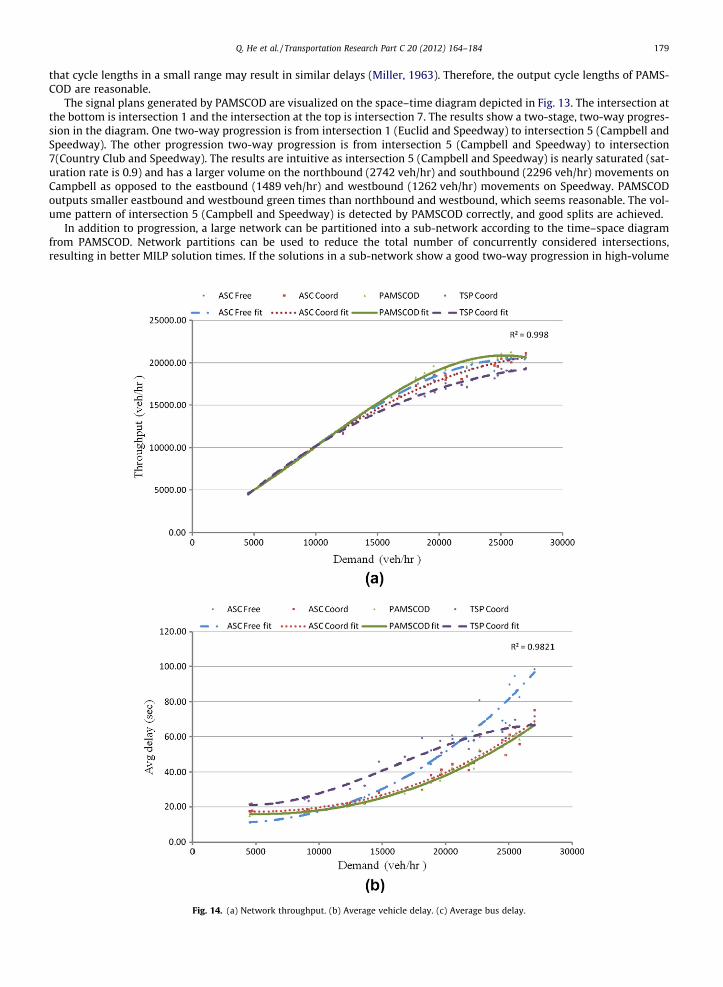
The signal plans generated by PAMSCOD are visualized on the space–time diagram depicted in Fig. 13. The intersection atthe bottom is intersection 1 and the intersection at the top is intersection 7. The results show a two-stage, two-way progres-sion in the diagram. One two-way progression is from intersection 1 (Euclid and Speedway) to intersection 5 (Campbell andSpeedway). The other progression two-way progression is from intersection 5 (Campbell and Speedway) to intersection7(Country Club and Speedway). The results are intuitive as intersection 5 (Campbell and Speedway) is nearly saturated (sat-uration rate is 0.9) and has a larger volume on the northbound (2742 veh/hr) and southbound (2296 veh/hr) movements onCampbell as opposed to the eastbound (1489 veh/hr) and westbound (1262 veh/hr) movements on Speedway. PAMSCODoutputs smaller eastbound and westbound green times than northbound and westbound, which seems reasonable. The vol-ume pattern of intersection 5 (Campbell and Speedway) is detected by PAMSCOD correctly, and good splits are achieved.

In addition to progression, a large network can be partitioned into a sub-network according to the time–space diagramfrom PAMSCOD. Network partitions can be used to reduce the total number of concurrently considered intersections,resulting in better MILP solution times. If the solutions in a sub-network show a good two-way progression in high-volume

Fig. 14. (a) Network throughput. (b) Average vehicle delay. (c) Average bus delay.

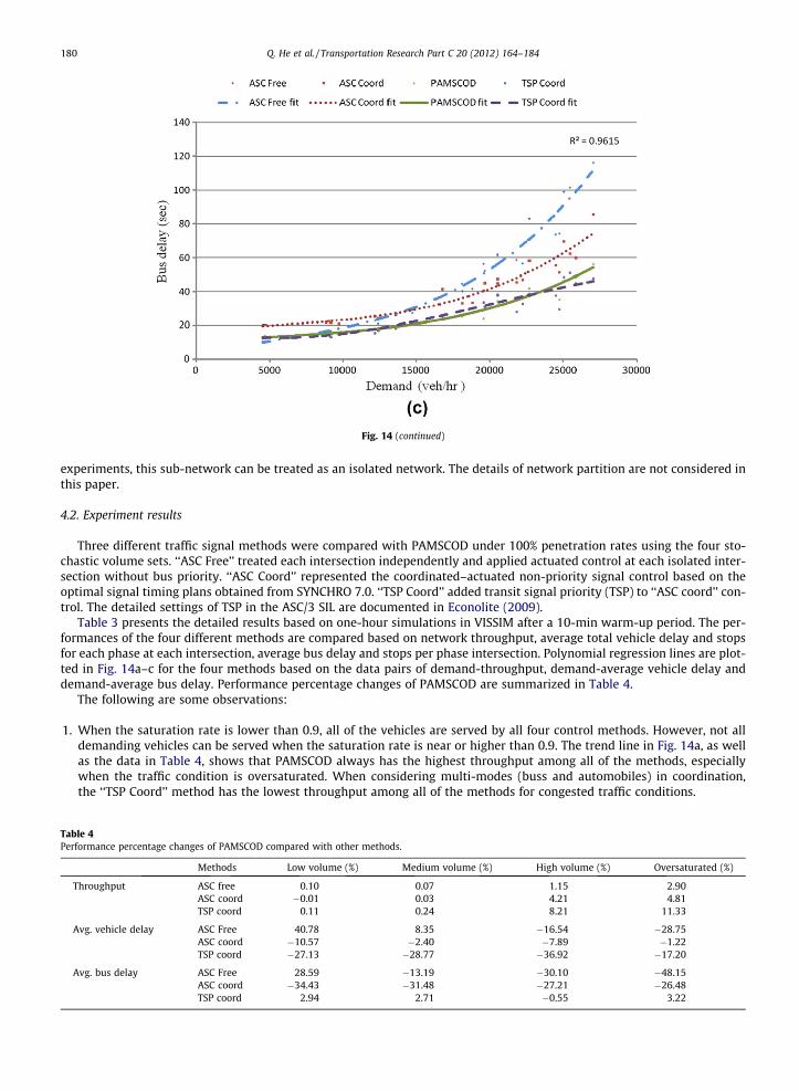
Fig. 14 (continued)

180 Q. He et al. / Transportation Research Part C 20 (2012) 164–184

experiments, this sub-network can be treated as an isolated network. The details of network partition are not considered inthis paper.

4.2. Experiment results

Three different traffic signal methods were compared with PAMSCOD under 100% penetration rates using the four sto-chastic volume sets. ‘‘ASC Free’’ treated each intersection independently and applied actuated control at each isolated inter-section without bus priority. ‘‘ASC Coord’’ represented the coordinated–actuated non-priority signal control based on theoptimal signal timing plans obtained from SYNCHRO 7.0. ‘‘TSP Coord’’ added transit signal priority (TSP) to ‘‘ASC coord’’ con-trol. The detailed settings of TSP in the ASC/3 SIL are documented in Econolite (2009).

Table 3 presents the detailed results based on one-hour simulations in VISSIM after a 10-min warm-up period. The per-formances of the four different methods are compared based on network throughput, average total vehicle delay and stopsfor each phase at each intersection, average bus delay and stops per phase intersection. Polynomial regression lines are plot-ted in Fig. 14a–c for the four methods based on the data pairs of demand-throughput, demand-average vehicle delay anddemand-average bus delay. Performance percentage changes of PAMSCOD are summarized in Table 4.

The following are some observations:

1. When the saturation rate is lower than 0.9, all of the vehicles are served by all four control methods. However, not alldemanding vehicles can be served when the saturation rate is near or higher than 0.9. The trend line in Fig. 14a, as wellas the data in Table 4, shows that PAMSCOD always has the highest throughput among all of the methods, especiallywhen the traffic condition is oversaturated. When considering multi-modes (buss and automobiles) in coordination,the ‘‘TSP Coord’’ method has the lowest throughput among all of the methods for congested traffic conditions.

Table 4Performance percentage changes of PAMSCOD compared with other methods.

Methods Low volume (%) Medium volume (%) High volume (%) Oversaturated (%)

Throughput ASC free 0.10 0.07 1.15 2.90ASC coord �0.01 0.03 4.21 4.81TSP coord 0.11 0.24 8.21 11.33

Avg. vehicle delay ASC Free 40.78 8.35 �16.54 �28.75ASC coord �10.57 �2.40 �7.89 �1.22TSP coord �27.13 �28.77 �36.92 �17.20

Avg. bus delay ASC Free 28.59 �13.19 �30.10 �48.15ASC coord �34.43 �31.48 �27.21 �26.48TSP coord 2.94 2.71 �0.55 3.22

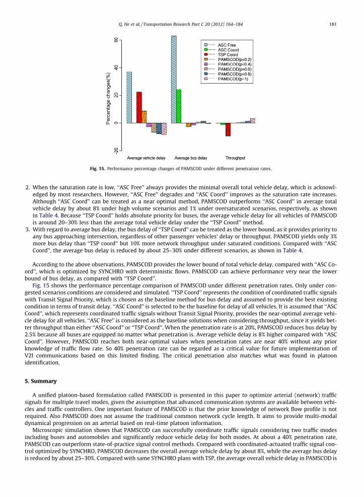
Fig. 15. Performance percentage changes of PAMSCOD under different penetration rates.

Q. He et al. / Transportation Research Part C 20 (2012) 164–184 181

2. When the saturation rate is low, ‘‘ASC Free’’ always provides the minimal overall total vehicle delay, which is acknowl-edged by most researchers. However, ‘‘ASC Free’’ degrades and ‘‘ASC Coord’’ improves as the saturation rate increases.Although ‘‘ASC Coord’’ can be treated as a near optimal method, PAMSCOD outperforms ‘‘ASC Coord’’ in average totalvehicle delay by about 8% under high volume scenarios and 1% under oversaturated scenarios, respectively, as shownin Table 4. Because ‘‘TSP Coord’’ holds absolute priority for buses, the average vehicle delay for all vehicles of PAMSCODis around 20–30% less than the average total vehicle delay under the ‘‘TSP Coord’’ method.

3. With regard to average bus delay, the bus delay of ‘‘TSP Coord’’ can be treated as the lower bound, as it provides priority toany bus approaching intersection, regardless of other passenger vehicles’ delay or throughput. PAMSCOD yields only 3%more bus delay than ‘‘TSP coord’’ but 10% more network throughput under saturated conditions. Compared with ‘‘ASCCoord’’, the average bus delay is reduced by about 25–30% under different scenarios, as shown in Table 4.

According to the above observations, PAMSCOD provides the lower bound of total vehicle delay, compared with ‘‘ASC Co-ord’’, which is optimized by SYNCHRO with deterministic flows. PAMSCOD can achieve performance very near the lowerbound of bus delay, as compared with ‘‘TSP Coord’’.

Fig. 15 shows the performance percentage comparison of PAMSCOD under different penetration rates. Only under con-gested scenarios conditions are considered and simulated. ‘‘TSP Coord’’ represents the condition of coordinated traffic signalswith Transit Signal Priority, which is chosen as the baseline method for bus delay and assumed to provide the best existingcondition in terms of transit delay. ‘‘ASC Coord’’ is selected to be the baseline for delay of all vehicles. It is assumed that ‘‘ASCCoord’’, which represents coordinated traffic signals without Transit Signal Priority, provides the near-optimal average vehi-cle delay for all vehicles. ‘‘ASC Free’’ is considered as the baseline solutions when considering throughput, since it yields bet-ter throughput than either ‘‘ASC Coord’’ or ‘‘TSP Coord’’. When the penetration rate is at 20%, PAMSCOD reduces bus delay by2.5% because all buses are equipped no matter what penetration is. Average vehicle delay is 8% higher compared with ‘‘ASCCoord’’. However, PAMSCOD reaches both near-optimal values when penetration rates are near 40% without any priorknowledge of traffic flow rate. So 40% penetration rate can be regarded as a critical value for future implementation ofV2I communications based on this limited finding. The critical penetration also matches what was found in platoonidentification.

5. Summary

A unified platoon-based formulation called PAMSCOD is presented in this paper to optimize arterial (network) trafficsignals for multiple travel modes, given the assumption that advanced communication systems are available between vehi-cles and traffic controllers. One important feature of PAMSCOD is that the prior knowledge of network flow profile is notrequired. Also PAMSCOD does not assume the traditional common network cycle length. It aims to provide multi-modaldynamical progression on an arterial based on real-time platoon information.

Microscopic simulation shows that PAMSCOD can successfully coordinate traffic signals considering two traffic modesincluding buses and automobiles and significantly reduce vehicle delay for both modes. At about a 40% penetration rate,PAMSCOD can outperform state-of-practice signal control methods. Compared with coordinated-actuated traffic signal con-trol optimized by SYNCHRO, PAMSCOD decreases the overall average vehicle delay by about 8%, while the average bus delayis reduced by about 25–30%. Compared with same SYNCHRO plans with TSP, the average overall vehicle delay in PAMSCOD is

182 Q. He et al. / Transportation Research Part C 20 (2012) 164–184

reduced by about 20–30%, and average bus delay is increased by only 3%. However, the throughput is increased by more than10% for congested cases, as compared with the TSP method.

Future research should mainly focus on how to reduce the solution times of PAMSCOD by considering network partition,reducing the complexity of the MILP or developing heuristic algorithms. In this paper, no prior knowledge of traffic flow isneeded in the model. However, it would be interesting to incorporate short term traffic prediction with signal control. Also itis a potential research topic to explore signal control optimization with online incident data in addition to traffic data.

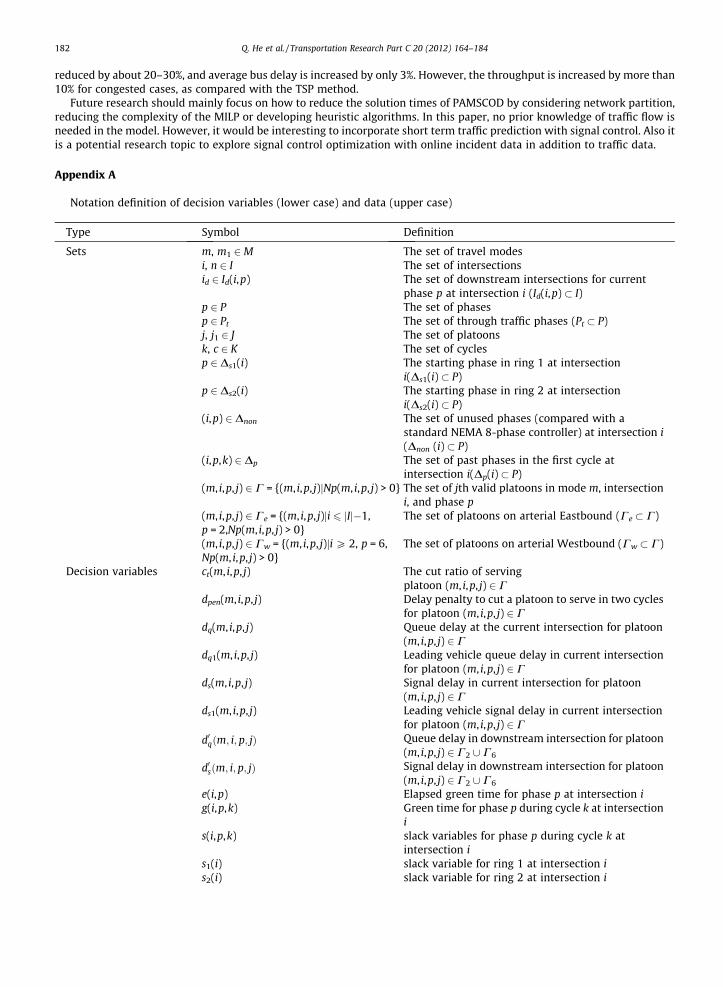
Appendix A

Notation definition of decision variables (lower case) and data (upper case)

Type S

ymbol Definition

Sets m

, m1 2M The set of travel modes i , n 2 I The set of intersections i d 2 Id(i,p) The set of downstream intersections for current

phase p at intersection i (Id(i,p) � I)

p 2 P The set of phases p 2 Pt The set of through traffic phases (Pt � P) j , j1 2 J The set of platoons k , c 2 K The set of cycles p 2Ds1(i) The starting phase in ring 1 at intersection

i(Ds1(i) � P)

p 2Ds2(i) The starting phase in ring 2 at intersection

i(Ds2(i) � P)

( i,p) 2 Dnon The set of unused phases (compared with a

standard NEMA 8-phase controller) at intersection i(Dnon (i) � P)

(

i,p,k) 2 Dp The set of past phases in the first cycle atintersection i(Dp(i) � P)

(

m, i,p, j) 2C = {(m, i,p, j)jNp(m, i,p, j) > 0} The set of jth valid platoons in mode m, intersectioni, and phase p

(

m, i,p, j) 2Ce = {(m, i,p, j)ji 6 jIj�1,p = 2,Np(m, i,p, j) > 0}

The set of platoons on arterial Eastbound (Ce � C)

(

m, i,p, j) 2Cw = {(m, i,p, j)ji P 2, p = 6,Np(m, i,p, j) > 0}

The set of platoons on arterial Westbound (Cw � C)

Decision variables c

t(m, i,p, j) The cut ratio of servingplatoon (m, i,p, j) 2C

d

pen(m, i,p, j) Delay penalty to cut a platoon to serve in two cyclesfor platoon (m, i,p, j) 2 C

d

q(m, i,p, j) Queue delay at the current intersection for platoon(m, i,p, j) 2C

d

q1(m, i,p, j) Leading vehicle queue delay in current intersectionfor platoon (m, i,p, j) 2 C

d

s(m, i,p, j) Signal delay in current intersection for platoon(m, i,p, j) 2C

d

s1(m, i,p, j) Leading vehicle signal delay in current intersectionfor platoon (m, i,p, j) 2 C

d

0qðm; i; p; jÞ Queue delay in downstream intersection for platoon(m, i,p, j) 2C2 [ C6

d

0sðm; i; p; jÞ Signal delay in downstream intersection for platoon(m, i,p, j) 2C2 [ C6

e

(i,p) Elapsed green time for phase p at intersection i g (i,p,k) Green time for phase p during cycle k at intersection

i

s (i,p,k) slack variables for phase p during cycle k at

intersection i

s 1(i) slack variable for ring 1 at intersection i s 2(i) slack variable for ring 2 at intersection i

Q. He et al. / Transportation Research Part C 20 (2012) 164–184 183

Appendix A (continued)

Type

Symbol Definition

t(i,p,k)

Starting time of phase p during cycle k atintersection i

v(i,p,k)

Phase duration time of phase p during cycle k atintersection i

h(m, i,p, j,k)

0–1 binary variables. Whether to serve platoon(m, i,p, j) in cycle k at current intersection (ifh(m, i,p, j,k) = 1, the platoon (m, i,p, j) is served incycle k at current intersection; else, not served incycle k)

h0(m, i,p, j,c)

0–1 binary variables. Whether to serve platoon(m, i,p, j) in cycle c at downstream intersection (ifh0(m, i,p, j,c) = 1, the platoon (m, i,p, j) is served incycle c at downstream intersection; else, not servedin cycle c)

Data

a Weighting factor for the sum of slack variables Cl(i,p) Link remaining storage capacity before solving the

MILP

Cr Reference cycle length (s) E(i,p) Elapsed green times for starting phase p at

intersection i (p 2 Ds1(i) [ Ds2(i)) (s)

Gmin(i,p) Minimal green time for phase p at intersection i (s) Gmax(i,p) Maximal green time for phase p during at

intersection i(s)

Fd(i,n) Platoon dispersion factor on link (i,n) Hp(m, i,p, j) Average headway of a platoon (m, i,p, j) (s) Hs(i,p) Saturation flow headway for phase p at intersection

i

Hs1 Saturation flow headway for a single lane (s) L(i,n) Link length between intersection i and n (m) Ls Average vehicle spacing in queue (m) M A large number Nl(i,p) Number of lanes at intersection i served by phase p Np(m, i,p, j) Number of vehicles in platoon (m, i,p, j) O1(i) Initial time for ring 1 at intersection i(s) O2(i) Initial time for ring 2 at intersection i(s) Pr(m, i,n) Percentage of a platoon arriving intersection n when

traveling from intersection i (Pr(m, i,n) 2 [0,1])

R(i,p) Red clearance time for phase p at intersection i (s) Sr(i,p) Saturation rate for phase p at intersection i (veh/h)

Ta(m, i,p, j)

Time arrival for leading vehicle in platoon (m, i,p, j)(s)

Taðm; i; p; jÞ

Time arrival for tail vehicle in platoon (m, i,p, j) (s) Tp(m, i,p, j) Green time needed to clear the platoon (m, i,p, j) (s) Tst Start-up lost time (s) Tt(m, i,n) Travel time between intersection i and n for mode m

(s)

Vf(m, i,p) Free flow speed for model m in phase p at

intersection i (m/s)

Vp(m, i,p, j) Average speed for platoon (m, i,p, j) (m/s) Vs Shock wave speed (m/s) W(m, i,p, j) Weight for platoon (m, i,p, j) Y(i,p) Yellow clearance time for phase p at intersection i

(s)

Z Allowable additional green rest time (s)

184 Q. He et al. / Transportation Research Part C 20 (2012) 164–184

References

Abu-Lebdeh, G., Benekohal, R., 1997. Development of traffic control and queue management procedures for oversaturated arterials. Transportation ResearchRecord: Journal of the Transportation Research Board 1603, 119–227.

Chaudhary, N., Abbas, M., Charara, H., 2006. Development and field testing of platoon identification and accommodation system. Transportation ResearchRecord: Journal of the Transportation Research Board 1978, 141–148.

Chaudhary, N., Chu, C., 2003. New PASSER Program for Timing Signalized Arterials. Texas Transportation Institute.Comert, G., Cetin, M., 2009. Queue length estimation from probe vehicle location and the impacts of sample size. European Journal of Operational Research

197 (1), 196–202.Daganzo, C., 1995. The cell-transmission model, Part II: network traffic. Transportation Research Part B: Methodological 29B (2), 79–93.Daganzo, C., 1994. The cell-transmission model: a simple dynamic representation of highway traffic. Transportation Research Part B: Methodological 28B

(4), 269–287.Dell’Olmo, P., Mirchandani, P., 1995. REALBAND: an approach for real-time coordination of traffic flows on networks. Transportation Research Record:

Journal of the Transportation Research Board 1494, 106–116.Econolite, 2009. Transit Signal Priority (TSP). User Guide for Advanced System Controller ASC/3.Gartner, N. et al, 1991. A multi-band approach to arterial traffic signal optimization. Transportation Research Part B: Methodological 25 (1), 55–74.Gaur, A., Mirchandani, P., 2001. Method for real-time recognition of vehicle platoons. Transportation Research Record: Journal of the Transportation

Research Board 1748, 8–17.Gazis, D., 1964. Optimum control of a system of oversaturated intersections. Operations Research 12 (6), 815–831.He, Q. et al., 2010. Heuristic algorithms to solve 0–1 mixed integer LP formulations for traffic signal control problems. In: 2010 IEEE International Conference

on Service Operations and Logistics, and Informatics. Qingdao, China, pp. 118–124.Head, K., 1995. Event-based short-term traffic flow prediction model. Transportation Research Record 1324, 105–114.Head, K., Gettman, D., Wei, Z., 2006. Decision model for priority control of traffic signals. Transportation Research Record: Journal of the Transportation

Research Board 1978, 169–177.Herrera, J.C., Bayen, A.M., 2010. Incorporation of Lagrangian measurements in freeway traffic state estimation. Transportation Research Part B:

Methodological 44 (4), 460–481.Hunt, P.B. et al, 1982. The SCOOT on-line traffic signal optimization technique. Traffic Engineering and Control 23 (4), 190–192.Husch, D., Albeck, J., 2003. Trafficware Intersection Capacity Utilization.Jiang, Y., Li, S., Shamo, D., 2006. A platoon-based traffic signal timing algorithm for major–minor intersection types. Transportation Research Part B:

Methodological 40, 543–562.Lin, W., Wang, C., 2004. An enhanced 0–1 mixed-integer linear program formulation for traffic signal control. IEEE Transactions on Intelligent

Transportation Systems 5 (5), 238–245.Little, J., 1966. The synchronization of traffic signals by mixed-integer linear programming. Operations Research 14 (4), 568–594.Little, J., Kelson, M., Gartner, N., 1981. MAXBAND: a program for setting signals on arteries and triangular networks. Transportation Research Record (795),

40–46.Lo, H., 2001. A cell-based traffic control formulation: strategies and benefits of dynamic timing plan. Transportation Science 35, 721–744.Lo, H., 1999. A novel traffic signal control formulation. Transportation Research Part A 33 (6), 433–448.Luk, J., 1984. Two traffic-responsive area traffic control methods: SCAT and SCOOT. Traffic Engineering and Control 25, 14–18.Miller, A., 1963. Settings for fixed-cycle traffic signals. Operational Research 14 (4), 373–386.Mirchandani, P., Head, K., 2001. A real-time traffic signal control system: architecture, algorithms, and analysis. Transportation Research Part C: Emerging

Technologies 9 (6), 415–432.Neumann, T., 2010. A cost-effective method for the detection of queue lengths at traffic lights. Traffic Data Collection and its Standardization. International

Series in Operations Research & Management Science. Springer, New York, pp. 151–160. <http://dx.doi.org/10.1007/978-1-4419-6070-2_10>.Research and Innovative Technology Administration, 2011. Connected Vehicle Research. <http://www.its.dot.gov/connected_vehicle/connected_vehicle.

htm> (accessed 31.03.11).Robertson, D.I., 1969. TRANSYT method for area traffic control. Traffic Engineering and Control 11 (6), 276–281.Smith, B.L., Venkatanarayana, R., Park, H., Goodall, N., Datesh, J., Skerrit, C., 2010. IntelliDriveSM Traffic Signal Control Algorithms. University of Virginia.Stamatiadis, C., Gartner, N., 1996. MULTIBAND-96: a program for variable bandwidth progression optimization of multiarterial traffic networks.

Transportation Research Record 1554, 9–17.Sun Tran, 2010. Sun Tran – Tucson, Arizona. <http://www.suntran.com/> (accessed 10.02.11).Trafficware, 2009. Synchro Studio 7.0 User’s Guide.Wallace, C. et al., 1998. TRANSYT-7F User’s Guide.Wasson, J. et al, 1999. Reconciled Platoon Accommodations at Traffic Signals. Purdue University, West Lafayette, IN.Yin, Y., 2008. Robust optimal traffic signal timing. Transportation Research Part B: Methodological 42 (10), 911–924.