TRANSPUTER BASED PARALLEL PROCESSING FOR GIS ANALYSIS: PROBLEMS AND POTENTIALITIES

Richard G. Healey and Ghazali B. DesaRegional Research Laboratory, Scotland

Department of GeographyUniversity of Edinburgh

Drummond Street Edinburgh EH8 9XP Scotland, U.K.

ABSTRACT

The availability of parallel processing computers based on large number of individual processing elements, offers the possibility of multiple orders of magnitude improvement in performance over the sequential processors currently used for GIS analysis. Before this potential can be realized, however, a number of problems must be addressed. These include assessment of the relative merits of different parallel architectures, choice of parallel programming languages and re-design of algorithms to allow effective distribution of the computational and i/o load between individual processors, so performance can be optimized. These problems are examined with particular reference to transputer-based parallel computers and some possible GIS application areas are discussed.

INTRODUCTION

The limitations of serial processors for handling computationally intensive problems in fields such as fluid dynamics, meteorological modelling and computational physics are well-known, but it is only comparatively recently that attention has been turned to this problem in the fields of remote sensing/image processing and GIS (Yalamanchi and Aggarwal 1985, Dangermond and Morehouse 1987). Parallel processing techniques, where one or many computational tasks are distributed across a number of processing elements, have been proposed as a solution to the problem (Verts and Thomson 1988). They offer the potential for orders of magnitude improvement in performance, which should allow real-time processing of very large datasets, with powerful modelling and visualization capabilities.

Since parallel processing hardware is still at an early stage of development and parallel programming methods are distinctly in their infancy, it is difficult to make firm statements about how GIS might avail itself of this new technology. More appropriate at this stage is an examination of several aspects of the overall problem. These aspects include evaluation of existing types of hardware and software for parallel processing and

90

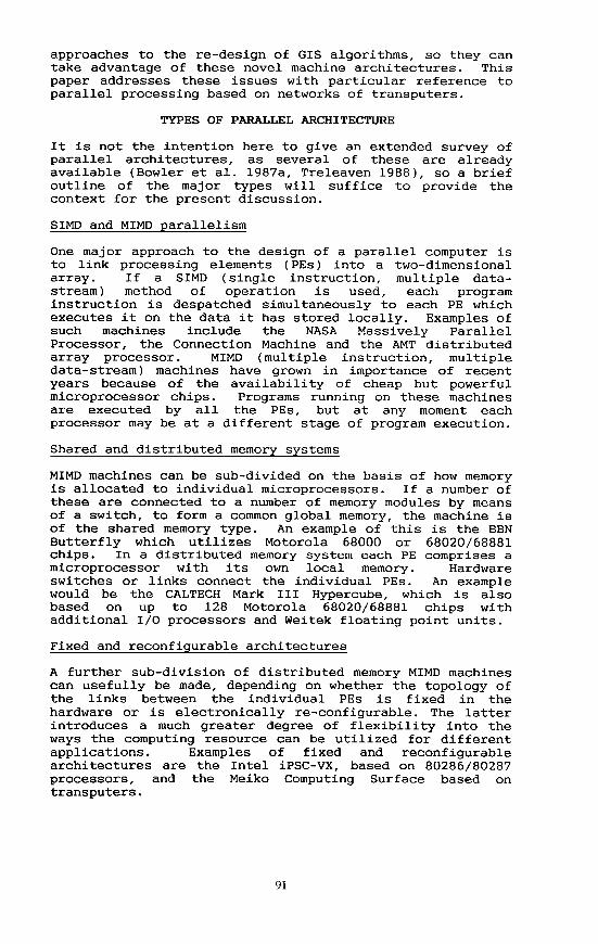
approaches to the re-design of CIS algorithms, so they can take advantage of these novel machine architectures. This paper addresses these issues with particular reference to parallel processing based on networks of transputers.

TYPES OF PARALLEL ARCHITECTURE

It is not the intention here to give an extended survey of parallel architectures, as several of these are already available (Bowler et al. 1987a, Treleaven 1988), so a brief outline of the major types will suffice to provide the context for the present discussion.

SIMP and MIMD parallelism

One major approach to the design of a parallel computer is to link processing elements (PEs) into a two-dimensional array. If a SIMD (single instruction, multiple data- stream) method of operation is used, each program instruction is despatched simultaneously to each PE which executes it on the data it has stored locally. Examples of such machines include the NASA Massively Parallel Processor, the Connection Machine and the AMT distributed array processor. MIMD (multiple instruction, multiple data-stream) machines have grown in importance of recent years because of the availability of cheap but powerful microprocessor chips. Programs running on these machines are executed by all the PEs, but at any moment each processor may be at a different stage of program execution.

Shared and distributed memory systems

MIMD machines can be sub-divided on the basis of how memory is allocated to individual microprocessors. If a number of these are connected to a number of memory modules by means of a switch, to form a common global memory, the machine is of the shared memory type. An example of this is the BBN Butterfly which utilizes Motorola 68000 or 68020/68881 chips. In a distributed memory system each PE comprises a microprocessor with its own local memory. Hardware switches or links connect the individual PEs. An example would be the CALTECH Mark III Hypercube, which is also based on up to 128 Motorola 68020/68881 chips with additional I/O processors and Weitek floating point units.

Fixed and reconfigurable architectures

A further sub-division of distributed memory MIMD machines can usefully be made, depending on whether the topology of the links between the individual PEs is fixed in the hardware or is electronically re-configurable. The latter introduces a much greater degree of flexibility into the ways the computing resource can be utilized for different applications. Examples of fixed and reconfigurable architectures are the Intel iPSC-VX, based on 80286/80287 processors, and the Meiko Computing Surface based on transputers.

91

TRANSPUTER-BASED PARALLEL PROCESSING

Since it is less widely known than the Motorola or Intel chip sets, it is useful to outline some of the particular features of the Transputer, which was designed with parallel processing in mind, before assessing some of the advantages and disadvantages of different parallel architectures.

The most recent version of the INMOS transputer, the T800 chip, contains a number of processing components. The first of these is a 10-MIPS 32-bit RISC processor linked at 80 MByte/Sec to 4K of on-chip RAM. In addition there is an integral 64-bit floating point unit capable of 1.5 Mflops. The chip has 4 20 MBit/sec INMOS links which can be directly connected to other transputers, together with an external memory interface with a bandwidth of 26.6 MByte/sec. The T800 is claimed to achieve more than five times the performance of the Motorola 68020/68881 combination on the Whetstone benchmark (Bowler et al. 1988).

The major vendor of transputer-based parallel computers is the UK firm Meiko Ltd. which has developed a modular, extensible and reconfigurable computer system called the 'Computing Surface'.

COMPARISON OF PARALLEL ARCHITECTURES

Given the difficulties of comparing supposedly similar serial processors, it is not surprising that comparison of parallel architectures, where there are many more parameters to consider, is a rather inexact science. Nonetheless, some major points relating to the different categories described above can be identified.

With respect to SIMD and MIMD architectures, testing of distributed array processors against transputer networks indicates that the former operate best with strongly structured algorithms which do not have independently branching chains of instructions. Requirements for very fast I/O and data comparison operations also favour SIMD machines. The two types both perform well for sorting, but transputer networks are superior for 3-d graphics and modelling requirements (Roberts et al. 1988).

For shared and distributed memory systems the picture is less clear, because shortcomings of specific hardware configurations may be compensated, to varying degrees by the use of different operating systems and programing methods. Several points need to be considered, however. Firstly, access to local memory is on average three times faster than to a global or shared memory. Secondly, the speed of interprocessor communication and thirdly, the relationship between the computational performance of each PE and the speed of interprocessor communication need to be taken into account. The usefulness of a particular architecture will then depend on the extent to which a

92

given problem can be decomposed into separate computational tasks, or requires access to a shared database of information (Bailie, 1988). The overall aims will be to minimize communications bottlenecks between processors, to get maximum utilization of each PE during the computation and to attain as nearly as possible a linear speed-up in processing time, as the number of processors used for a particular set of calculations is increased. Distributed memory systems, such as the transputer network, are proving popular because of fast memory access, but difficulties may arise for such systems in terms of communications overheads, if large amounts of data require to be transferred between processors.

Comparison between fixed and reconfigurable architectures is more straightforward, in that the latter is undoubtedly to be preferred, for two main reasons. Firstly, it allows the machine to 'mimic' other architectures, such as a SIMD or a hypercube, for comparative purposes. Secondly, it permits the overall computational resources to be divided into 'domains' of different sizes, so parts of the machine can be used for development while others are engaged in large scale computation.

Finally, the cost-effectiveness of parallel architectures involving large numbers of PEs, compared to single or multiple vector processors much be addressed. The parallel approach has an initial advantage because it is scalable from a small number of PEs, costing a few thousand dollars, to top-end Computing Surfaces costing several millions. In addition, using the unit comparison of megaflops/megadollar, a transputer-based machines seems to have approximately a five-fold improvement in cost effectiveness compared to a CRAY X-MP/48, with similar floating point performance (Bowler et al. 1987b).

These considerations indicate that reconfigurable, distributed memory MIMD machines such as the Meiko Computing Surface have a wide range of advantages, with potential limitations only in relation to interprocessor communication and extreme high-end reqirements for floating point performance. As a result, the Meiko machine was chosen as the basis for the Edinburgh Concurrent Supercomputer Project. The first phase of this has resulted in the installation of a Meiko machine with 200 transputers, each with 4 MB of local memory, together with a filestore and specialized graphics peripherals. Future project phases will allow the installation of large numbers of additional transputers, until the machine reaches its target size of at least 1024 processors, with 10,000 MIPS total processing power, 4 GBytes of distributed memory and an expected rating in excess of 1 Gflop. This will make it one of the most powerful supercomputers in Europe. The machine is jointly managed by the University Computing Service and the Department of Physics, but is in use by a variety of other research groups also.

93

PARALLEL PROGRAMMING LANGUAGES

Although parallel hardware has demonstrably reached the stage where a range of applications for large scale CIS processing can be envisaged, the position is less clear in terms of operating systems and programming languages.

Since parallel machines generate many new problems of system management, they have tended to be built with special purpose operating systems, which is a first major obstacle to software development activity of any kind! In the case of the Meiko this problem has now been resolved by the development of a UNIX System V compatible operating system for development work.

The second obstacle is the lack of support for parallel programming constructs in existing languages used for GIS software, specifically FORTRAN, C and to some extent PASCAL, although FORTRAN 8X is expected to include such facilities in the future. At present, there are three alternative methods of circumventing the problem:

i) Addition of new constructs into language compilers running on parallel machines

ii) Use of new languages, such as ADA or OCCAM, which support parallel programming directly

iii) Use of existing languages within a communications 'harness' provided by languages like OCCAM to allow access to parallel facilties.

In relation to the first alternative, a 'parallel' C compiler has been announced for the transputer, but problems of standardization are likely to plague this approach. The second alternative offers promise because the transputer was designed to run OCCAM, a language for parallel programming based heavily on Hoare's work on communicating sequential processes (Jesshope 1988). The language has particular strengths in facilities for message passing along OCCAM channels, but is limited in its support for the variety of data structures found in existing sequential languages. ADA, by contrast, supports parallel programming through its tasking model, while having a wealth of data structures. It also provides constructs to support the use of sound software engineering techniques (Sommerville and Morrison 1987). An ADA compiler for the transputer is currently under development and this avenue for future work will be explored when the tools become available. The final alternative is the one which is most heavily used at present on the Meiko processor, particularly for FORTRAN in an OCCAM harness. The FORTRAN implementation allows block input and output of data arrays between FORTRAN programs running on different processors, across OCCAM channels communicating over the transputer hardware links. This approach is satisfactory in the short term for testing alternative parallel algorithms or re using existing code, to take advantage of the substantial

94

increase in processing power on a parallel machine. It is not, however, a suitable approach for the implementation of large programming projects, designed to produce reliable and maintainable software that makes effective use of parallel processing techniques.

The shortcomings in available facilities and standards for parallel programming languages require to be addressed urgently if progress in the use of the hardware is not be hampered. While these shortcomings make it difficult to port existing packages, the situation may not be entirely disadvantageous, as it allows attention to be focussed at present on research into methods of parallelization of algorithms. Development of effective approaches for different kinds of algorithms is fundamental to the proper utilization of parallel processing techniques.

PARALLELIZATION OF ALGORITHMS

It is apparent from the earlier discussion that algorithms appropriate for one kind of parallel architecture may be unsuitable for another. This examination of parallelization methods will be restricted to distributed memory MIMD machines.

Although architecture dependent at the level of specific implementation, several general points about the relationships between serial and parallel algorithms can still be made (Miklosko and Kotov 1984):

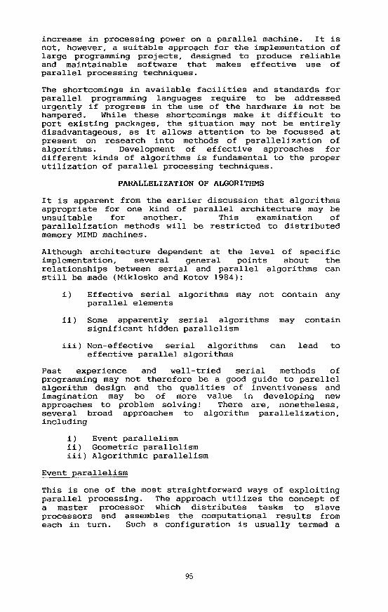
i) Effective serial algorithms may not contain any parallel elements

ii) Some apparently serial algorithms may contain significant hidden parallelism

iii) Non-effective serial algorithms can lead to effective parallel algorithms

Past experience and well-tried serial methods of programming may not therefore be a good guide to parellel algorithm design and the qualities of inventiveness and imagination may be of more value in developing new approaches to problem solving! There are, nonetheless, several broad approaches to algorithm parallelization, including

i) Event parallelismii) Geometric parallelismiii) Algorithmic parallelism

Event parallelism

This is one of the most straightforward ways of exploiting parallel processing. The approach utilizes the concept of a master processor which distributes tasks to slave processors and assembles the computational results from each in turn. Such a configuration is usually termed a

95

'task farm' (Bowler et al. 1987t>). In the simplest kinds of problem, each slave processor runs the same code against its own specific dataset. When the processor array is large and each processor individually very powerful, as on the Meiko machine, it can be difficult to achieve data input rates sufficiently, high to keep the machine busy. Conversely, where the computational load is very high but the data input more restricted the Meiko delivers extremely high performance. A good example of this type of problem is ray tracing for the display of complex 3-d objects. Since each light ray being followed is independent, the algorithm is highly parallel. While such algorithms have important application for visualization problems in CIS, many other CIS processing requirements are not of this form.

Geometric parallelism

This is a very natural kind of parallelism for CIS algorithms, as it requires that the problem space be divisible into sub-regions, within which local operations are performed. Calculations performed on elements near the boundaries of sub-regions will generally require information from neighbouring sub-regions. This emphasis on algorithm localization matches an approach which can be found, for instance, in the Intergraph TIGRIS system, for interactive editing of topological data structures (Herring1987) and in the inward spiral algorithm for TIN generation (McKenna 1987).

Since individual sub-regions will be handled by different processors, boundary data must be passed between them, introducing a communications overhead. It is therefore important, with the current level of development of distributed memory MIMD machines, to define sub-regions such that the amount of within region processing is maximized and the between region communication is minimized. It is also advisable to locate neighbouring regions on physically adjacent processors. (Bowler et al.1988).

The four available hardware links on each transputer are sufficient for two-dimensional geometric parallelism, but even for the simplest three-dimensional case with sub- regions forming cubes, each sub-region will hve six boundary faces. This can be matched in the hardware by connecting multiple transputers as 'supernodes' to yield six or more links (Jesshope 1988).

For geometric parallelism it is also necessary to consider the way in which the overall processing operation and communication between processors is organized. If a tightly synchronous model is used, a master processor communicates with each sub-region processor to determine when all have completed their local computations for a given step. At this point an exchange of boundary information takes place before proceeding with the next computational step. This approach generally produces

96

inefficient hardware utilization. The loosely synchronous model, where boundary information is exchanged as soon as one processor is ready to provide it and its neighbour is ready to receive it, is to be preferred if processor workloads are broadly similar. If workloads vary significantly, as might be expected for CIS applications, complex asynchronous behaviour may result, leading to unpredictable levels of inefficiency (Norman 1988). One solution to this is to recast the problem to allow improved dynamic balancing of the workload, perhaps by assigning non-contiguous portions of the overall space to individual processors. This approach has been used effectively for three-dimensional medical imaging (Stroud and Wilson 1987) and has immediate application for voxel-based processing of geosciences data (cf. Kavouras and Masry 1987).

Algorithmic parallelism

With this approach, each individual processor performs a specific task on blocks of data which pass through the processor network in a production line fashion. Though attractive as a concept, algorithmic parallelism encounters difficulties at the implementation stage which tend to reduce its efficiency. These include communication and configuration problems. In the former case, each processor has to receive different initialization instructions for its specific portion of the computational task. In the latter case, one configuration of inter-processor linkages may be appropriate for some stages of the work and inappropriate for others. This will remain a problem until the technology for dynamic reconfiguration of processor arrays becomes available. While quantitative comparisons are very hard to find, experiments at Southampton University on Monte Carlo simulations suggest that geometric parallelism gives a much better approximation to linear speed-up as the number of processors is increased, than does algorithmic parallelism (Bowler et al. 1987a). Whether a similar conclusion would apply to parallel implementations of topological map processing must be left as a subject for future investigation!

CONCLUSIONS

Parallel processing hardware is now reaching the stage where extremely high performance computers can be built in a modular and cost effective way, particularly if powerful processing chips with good communications links, such as the transputer, are used. As usual the pace of algorithm research and software development is lagging significantly behind the hardware. Of the recognised approaches to algorithm construction, geometric parallelism, possibly combined with limited algorithmic parallelism, offers the most promising route for initial work in parallel CIS processing. Early areas of investigation using the Meiko Computing Surface include computationally intensive three didmensional CIS problems and in future, polygon overlay algorithms. Beyond these a whole range of novel and indeed exciting possibilities present themselves for parallel

97

search on large spatial databases, real-time data structure conversion, and new approaches to visualization and user interfacing.

REFERENCES

Baillie, C.F. 1988, Comparing Shared and Distributed Memory Computers: Parallel Computing, Vol. 8, pp. 101-110.

Bowler, K.C., Kenway, R.D., Pawley, G.S. and Roweth, D. 1987a, An Introduction to OCCAM 2 Programming, Chartwell- Bratt, Lund.

Bowler, K.C., Bruce, A.D., Kenway, R.D., Pawley, G.S. and Wallace, D.J. 1987b, Exploiting Highly Concurrent Computers for Physics : Physics Today, October Edition.

Bowler, K.C., Kenway, R.D., Pawley, G.S. and Roweth D. 1988, OCCAM 2 Programming Course Notes, Publications, Dept. of Physics, University of Edinburgh.

Dangermond, J. and Morehouse, S. 1987, Trends in Hardware for Geographic Information Systems : Proceedings Auto-Carto 8, pp. 380-385, ASPRS/ACSM, Falls Church, Va.

Herring, J. 1988, TIGRIS : Topologically Integrated Geographic Information System : Proceedings Auto-Carto 8, pp. 282-291, ASPRS/ACSM, Falls Church, Va.

Jesshope, C. 1988, Transputers and Switches as Objects in OCCAM : Parallel Computing, Vol. 8, pp. 19-30.

Kavouras, M. and Masry S. 1987, An Information System for Geosciences : Design Considerations : Proceedings Auto- Carto 8, pp. 336-345, ASPRS/ACSM, Falls Church, Va.

McKenna, D. 1987, The Inward Spiral Method: An Improved TIN Generation Technique and Data Structure for Land Planning Applications : Proceedings Auto-Carto 8, pp. 670-679, ASPRS/ACSM, Falls Church, Va.

Miklosko, J. and Kotov, V.WE. (Eds.) 1984, Algorithms, Software and Hardware of Parallel Computers, Springer- Verlag, Berlin.

Norman, M. 1988, Asynchronous Communication Course Notes, Dept. of Physics, University of Edinburgh.

Roberts, J.B.G., Harp, J.G., Merryfield, B.C., Palmer, K.J., Simpson P., Ward, J.S. and Webber H.C. 1988, Evaluating Parallel Processors for Real-time Applications : Parallel Computing, Vol. 8, pp. 245-254.

Sommerville, I. and Morrison, R. 1987, Software Development with ADA, Addison-Wesley, Reading. Mass.

Stroud, N. and Wilson, G. (Eds.) 1987, Edinburgh Concurrent Supercomputer Project Newsletter No. 3, Edinburgh

98

University Computing Service.

Treleaven, P.C. 1988, Parallel Architecture Overview : Parallel Computing, Vol. 8, pp. 59-70.

Verts. W.T. amd Lee, C. 1988. Parallel Architectures for Geographic Information Systems, Technical Papers ACSM-ASPRS Annual Convention, Vol. 5, pp. 101-107, ACSM/ASPRS, Falls Church, Va.

Yalamanchi S. and Aggarwal, J.K. 1985, Analysis of a Model for Parallel Image Processing : Pattern Recognition, Vol. 18, pp. 1-16.

99

UNIFORM GRIDS:A TECHNIQUE FOR INTERSECTION DETECTION

ON SERIAL AND PARALLEL MACHINES

Wm. Randolph FranklinChandrasekhar Narayanaswaml

Mohan KankanhalllDavid Sun

Meng-Chu ZhouPeter YF Wu

Electrical, Computer, and Systems Engineering Dept.,6026J.E.C.,

Rensselaer Polytechnic Institute, Troy, NY, 12180, USA,

(518) 276-6077,Internet: Franklin@CS.RPI.EDU, Bltnet: WRFRANKL@RPITSMTS,

Fax: (518) 276-6003, Telex: 6716050 RPI TROU.

ABSTRACT

Data structures which accurately determine spatial and topological relationships in large databases are crucial to future developments in automated cartography. The uniform grid technique presented here offers an efficient solution for intersection detection, which is the key issue in many problems including map overlay. Databases from cartog raphy, VLSI, and graphics with up to 1 million edges are used. 1,819,064 edges were processed to find 6,941,110 intersections in 178 seconds on a Sun 4/280 workstation. This data structure is also ideally suited for implementation on a parallel machine. When executing on a 16 processor Sequent Balance 21000, total times averaged ten times faster than when using only one processor. Finding all 81,373 intersections in a 62,045 edge database took only 28 seconds elapsed time. These techniques also appear applicable to massively parallel SIMD (Single Instruction, Multiple Data Stream) com puters. We have also used these techniques to implement a prototype map overlay sys tem and performed preliminary tests on overlaying 2 copies of US state boundaries, with 3660 edges in total. Finding all the intersections, given the edges in memory, took only 1.73 seconds on a Sun 4/280. We estimate that the complete overlay would take under 20 seconds.

INTRODUCTION

Algorithms specific to polyline intersection are particularly important for cartographic purposes. The classic problem of map overlay is a good example where edge intersection forms the core of the algorithm. The results of this paper are also useful in diverse dis ciplines such as graphics and VLSI design.

We are given thousands or millions of small edges, very few of which intersect, and must determine the pairs of them that do intersect. Clearly, a quadratic algorithm com paring all \~2\ pairs is not acceptable.

Useful line intersection algorithms often use sweep line techniques, such as in Nievergelt and Preparata (1982), and Preparata and Shamos (1985). Chazelle and Edelsbrunner (1988) have an algorithm that finds all K intersections of N edges in time F = Q(K+N\ogN). This method is optimal in the worst case, and is so fast that it

100

cannot even sort the output intersections. However, this method has some limitations. First, it cannot find all the red-blue intersections in a set of red and blue edges without finding (or already knowing) all the red-red and blue-blue intersections. Second, it is inherently sequential.

Alternative data structures, based on hierarchical methods such as quadtrees, have also been used extensively, Samet (1984). They are intuitively reasonable data structures to use since they subdivide to spend more time on the complicated regions of the scene. An informal criticism of their overuse in Geographic Information Systems in given in Waugh (1986). A good general reference on cartographic data structures is Peucker (1975).

Since cartographers deal with vast amounts of data, the speed and efficiency of the algo rithms are of utmost importance. With the advent of parallel and supercomputers, effi cient parallel algorithms which are simple enough to implement, are gaining importance. Since this field is relatively new, few implementable algorithms exist. Some of the related parallel algorithms in computational geometry are as follows. Aid (1985) describes some parallel convex hull algorithms. Evans and Mai (1985) and Stojmenovic and Evans (1987) present parallel algorithms for convex hulls; however they require a MIMD machine, and have tested on only a few processors. Aggarwal et al (1985) give parallel algorithms for several problems, such as convex hulls and Voronoi diagrams. They assume a CREW PRAM (concurrent read exclusive write, parallel random access machine). This is a MIMD model. No mention is made of implementation. Although it is not mentioned in those papers, randomized algorithms, such as described by dark- son (1988a), and Clarkson and Shor (1988b) appear to lend themselves to parallelization sometimes. Yap (1987) considers general questions of parallelism and computational geometry. Hu and Foley (1985), Reif and Sen (1988), and Kaplan and Greenberg (1979) consider hidden surface removal. Scan conversion is considered by Fiume, Four- nier, and Rudolph (1983). For realistic image synthesis see Dippe and Swensen (1984).

This paper concentrates on an alternative data structure, the uniform grid. Here, a flat, non-hierarchical grid is superimposed on the data. The grid adapts to the data since the number of grid cells, or resolution, is a function of some statistic of the input data, such as average edge length. Each edge is entered into a list for each cell that it passes through. Then, in each cell, the edges in that cell are tested against each other for inter section. The grid is completely regular and is not finer in the denser regions of the data.

The uniform grid (in our use) was first presented in Franklin (1978) and was later expanded by Franklin, Akman, and Wu (1980), (1981), (1982), (1983), (1984), (1985), (1987), and Wu(1988) . The latter two papers used extended precision rational numbers and Prolog to implement map overlay. Geometric entities and relationships are represented in Prolog facts and algorithms are encoded in Prolog rules to perform data processing. Multiple precision rational arithmetic is used to calculate geometric intersec tions exactly and therefore properly identify all special cases of tangent conditions for proper handling. Thus topological consistency is guaranteed and complete stability in the computation of overlay is achieved.

In these papers the uniform grid was called an adaptive grid. However, there is another, independent and unrelated, use of the term adaptive grid in numerical analysis in the iterative solution of partial differential equations. Our papers present an expected linear time object space hidden surface algorithm that processed 10,000 random spheres packed ten deep in 383 seconds on a Prime 500. The idea was extended to a fast haloed line algorithm that was tested on 11,000 edges. The concept was applied to other prob lems such as point containment in polygon testing. Finally it was used, in Prolog and with multiple precision rational numbers in the map overlay problem in cartography.

This present paper presents experimental evidence that the uniform grid is an efficient means of finding intersections between edges in real world data. The uniform grid is similar to a quadtree is the same sense that a relational database schema is similar to a

101

hierarchical schema. The power of relational databases, derived from their simplicity and regularity, is also becoming apparent.

The uniform grid data structure is also ideally suited to execution on a parallel machine because of the simple data structures. Also, it is more numerically robust than sweep- line algorithms that have problems. This is of importance in the cartographic domain because numerical instability can easily introduce topological inconsistencies which tend to be difficult to rectify.

The uniform grid technique is fairly general and can be used on a variety of geometric problems such as computing Voronoi diagrams, convex hull determination, Boolean combinations of polygons, etc.

INTERSECTION ALGORITHM

Assume that we have N edges of length L independently and identically distributed (i.i.d.) in a 1 x 1 screen. We place a G x G grid over the screen. Thus each grid cell isof size x . The grid cells partition the screen without any overlaps or omissions. The intersection algorithm proceeds as follows.

1. For each edge, determine which cells it passes through and write ordered pairs (cell number, edge number).

2. Sort the list of ordered pairs by the cell number and collect the numbers of all the edges that pass through each cell.

3. For each cell, compare all the edges in it, pair by pair, to test for intersections. If the edges are a priori known to be either vertical or horizontal, the vertical edges are compared with the horizontal edges only. To determine if a pair of edges inter sect, we test each edge's endpoints against the equation of the other edge. We ignore calculated intersections that fall outside the current cell. This handles the case of some pair of edges occurring together in more than one cell.

Fig !( ). USA Map - Shifted and Overlaid on itself Fig l(b). Chickamauga Area - All 4 overlays

102

THEORETICAL ANALYSIS

Let Ncit be the number of cells that an average edge passes through. The determination of Nc/t is similar to the Buffon's Needle Problem, McCord (1964). A simple analysis shows that,

Nelt = (1 + ^LG) (E9.l)

Then Np , the total number of (cell, edge) pairs isNp = N(l + — LG) (Eg. 2)

ITThe average number of edges per cell is

The time to calculate the (cell, edge) pairs isTI = «Np (Eq.S)

where a is a constant. The time to test the edges for intersections is aboutJ2 = 3 G 2 Ne/c (Nc,e - 1) (£0.6)

where P is a constant. The overhead for processing the cells isr3 = -/G 2 (Eq.r)

where -y is a constant, and the total time isr =

This is minimized if the 2 fastest terms in the sum grow at the same speed, which occurs

when G = min 18V#, -£-1 for some 8.

What about some cells being denser since the edges are randomly distributed? Since the time to process a cell depends on the square of the number of edges in that cell, an uneven distribution might increase the total time. However, since the edges are assumed independent, the number of edges per cell is Poisson distributed, and the expected value of the square of the number of edges equals the square of the expected number of edges. Therefore the expected time doesn't increase.

RESULTS

Edge Intersection

For each data set we tried many values of G to learn the variation of time with G. Table 1 shows the results from intersecting the 116896 edges in all the 4 overlays of the Chi- kamauga DLG (Figure 1). There are 144,666 intersections in all, and the best time is 37 seconds with a 325 x 325 grid. The time is within 50% of this for grids from 175 x 175 up to 1000 x 1000, which shows the extreme insensitivity of the time to the grid size. This is why real scenes with dense and sparse areas can be accommodated efficiently.

For the USA state boundaries shifted and overlaid on themselves, the execution time is within 20% of the optimum from about G = 40 to G = 400 and is within a factor of two of the optimum from about G = 20 to G = 700. Outside these limits, the execution time starts to rise quickly.

The economy of the grid structure is shown by the fact that the number of comparisons between pairs of edges needed to isolate the intersections is about twice the number of the edges when using the optimal grid resolution. This behavior was also observed in hidden surface algorithm described in earlier publications. There is not much room for

103

No. of edges 116896Avg. edge length 0.00231Standard deviation 0.0081Xsects. by end pt. coincidence 13S87SXsects. by actual equation soln 8791Total intersections 144666

Grid Size

5080

100125175200275325400500625800

10002000

Pairs

131462140407146389153492168341175791197815212282

' 234372263646300413351891410589704147

P/Cell

52.58521.93914.6399.8235.4974.3952.6162.0101.4651.0550.7690.5500.4110.176

P/Edge

1.1251.2011.2521.3131.4401.5041.6921.8162.0052.2552.5703.0103.5126.024

Grid Time

4.334.504.724.885.436.708.457.378.37

10.1811.7214.5217.7231.05

Sort Time

3.673.934.224.324.826.137.686.187.157.788.92

10.7712.9322.92

Xsect Time

182.0490.7567.3151.3636.2235.1831.7823.6021.8220.6220.2221.3723.0529.57

Total Time

190.0499.1876.2560.5646.4648.0147.9137.1537.3338.5840.8546.6553.7083.53

Table 1: Intersecting 116,896 Edges of the Chikamauga DLG

further improvement by a hierarchical method.

The largest cartographic database was the 116,896 edges of the Chikamauga Digital Line Graph (DLG) from the USGS sampler tape. The average edge length was 0.0022 and the standard deviation 0.0115, so the edges were quite variable. We used a 325x325 grid to find all 144,666 intersections in 37.15 seconds on a Sun 4/280. Other results are listed in Franklin, Chandrasekhar, Kankanhalli, Seshan, Akman (1988).

One of our examples consisted of 1,819,064 edges, with an average length of 0.0012, forming a complete VLSI chip design. We found all 6,941,110 intersections in 178 seconds. In this case, the program was optimized to use the orthogonality of the edges. The edges' lengths were quite variable, with the standard deviation being over 30 times the mean. This example illustrates the generality of this method and its applicability to other areas besides cartography.

Execution in Parallel

The uniform grid method is ideally suited to execution on a parallel machine since it mostly consists of two types of operations that run well in parallel: applying a function independently to each element of a set to generate a new set, and sorting. Determining which cells each edge passes through is an example of the former operation.

We implemented several versions of the algorithm on a Sequent Balance 21000 com puter, which contains 16 National Semiconductor 32000 processors, Sequent (1986), KaIIstrom(1988) and compared the elapsed time when up to 15 processors were used to

104

the time for only one processor, Kankanhalli (1988). We used the 'data partitioning' paradigm of parallel programming which involves creating multiple, identical processes and assigning a portion of the data to each process. The edges are distributed among the processors to determine the grid cells to which each edge belongs and then the cells are distributed among the processors to compute the intersections. Since the Sequent Balance 21000 is a shared memory parallel computer, shared data structures is the communica tion mechanism for the processors. The synchronization of the processors is achieved by using atomic locks. Basically, the concept of 'local processing' has been adopted in this algorithm to achieve parallelism.

There were several different ways of implementing the uniform grid data structure. First, we had a G 2MP array of cells, where G is the grid size, M is the maximum number of edges per cell per processor and P is the number of processors. However this implementation took up a lot of memory space though it obviated the use of locks. Then, G 2 array of linked lists was used. This also did not require locking but it was slow because of the dynamic allocation of shared global memory. Then it was implemented using a linked list of (cell,edge) pairs but this also was slow because of dynamic memory allocation. Finally a G 2Af array implementation was made which used atomic locks. This implementation gave the best results.

The speedup ratios range from 8 to 13. Figure 2 shows the results from processing 3 overlays of the United State Geological Survey Digital Line Graph, totaling 62,045 edges. 81,373 intersections were found. The time for one processor was 273 seconds, and for IS processors was 28 seconds, for a speedup of about 10. This is a rate of 7.9 million edges and 10.5 million intersections per hour. For other data sets, these extra polated times would depend on those data sets' number of intersections per edge.

The speedup achieved for any parallel algorithm is dependent on the amount of inherently sequential computation in the algorithm, the hardware contention imposed by the competing processors, the overhead in creating multiple processes and the overhead in synchronization & communication among the multiple processes. We believe that the first factor is not dominant when using the uniform grid technique. The large speedups achieved show that the other three factors also do not affect the performance signifi cantly. Finally, the speedup, as a function of the number of processors, was still rising smoothly at 15 processors. This means that we should achieve an even bigger speedup on a more parallel machine.

Map Overlay

We are implementing a complete map overlay package in C on a Sun workstation. The input and output are in a simplified form of the Harvard Odyssey cartographic database format. The preliminary version emphasizes clarity at the expense of speed by representing the process as a pipeline of several sequential processes. Each process writes its output to a temporary ASCII file for the next process to read, thus incurring repeated I/O costs. The stages are as follows.

1. Deform: In this stage chains are broken into edges.

2. Intersect: This stage finds all intersection points between edges.

3. Connect: This stage breaks up original chains into new chains, additional break points being made at the intersection points.

4. Link: This stage calculates and sorts the angles between each of the chains at each node and the x-axis.

5. Form: This stage recognizes all polygons formed by the new chains.

105

Total TIM

(iMMdi)

300

UO

200

UO

100

50

0

-

- ',

1 I 1 I 1) 1 6 » 11 U

Nnmbw Of Proctuora(t)

Up

Numbtr 0( Proetiiort

Fig 2. Time and Speedup when intersecting the 62045 edges in the Roads & Trails, Railroads and Pipes and Transmission Lines 9verlays of The Chickamauga DLG in Parallel on 1 to 15 Processors. Grid size = 250. 81,373 intersections found.

6. Display: This displays the resulting overlaid map along with labels for each recog nizable polygon.

7. Timer. This sums up the time each of the first S modules takes to complete each individual task.

One, possibly controversial, decision, was to split the chains into the individual edges at the start. This makes the data more voluminous, but much simpler, since now the ele ments have a fixed length. After we have intersected all the edges, and split them into pieces which are the edges of the result, it is easy to reform the output chains.

Another advantage of using individual edges is that the algorithm will be easier to

106

implement on a parallel machine for even greater speed.

We have implemented the algorithm partly on a Sun 3/50 and part on a Sun 4/280. Test ing all 3660 edges in both input maps to find intersections takes only 1.73 seconds on the Sun 4.

CONCLUSION

Our technique has been successfully used for the important problem of map overlay which occurs in cartography. The results indicate that this is a very robust general tech nique which is fast and simple. It is evident from this research that simple solutions are often faster than theoretically efficient but convoluted and complicated methods. Also, the power of randomized techniques in algorithm design for real world problems is now being appreciated. Our algorithm is parallelizable and shows very good speedup with minimal auxiliary data structures.

As mentioned before, we are investigating other problems where the uniform grid tech nique may be applied for inventing parallel algorithms. We feel that the uniform grid technique is a good technique for parallel geometric computation in the future.

ACKNOWLEDGEMENTS

This work was supported by the National Science Foundation under PYI grant no. CCR-8351942. It used the facilities of the Computer Science Department funded by a DoD equipment grant, and the Rensselaer Design Research Center.

REFERENCES

Aggarwal, Alok, Chazelle, Bernard, Guibas, Leo, O'Dunlaing, Colm, and Yap, Chee (1985) "Parallel Computational Geometry," Foundations of Computer Science - 25th Annual Symposium, pp. 468-477 (1985).

Akl, Selim G. (1985) "Optimal Parallel Algorithms for Selection, Sorting, and Com puting Convex Hulls," pp. 1-22 in Computational Geometry, ed. Godfried T. Toussaint (1985), pp. 1-22.

Chazelle, Bernard and Edelsbrunner, Herbert (1988) "An Optimal Algorithm for Intersecting Line Segments in the Plane," Foundations of Computer Science - 29th Annual Symposium, White Plains (October 1988).

Chrisman, T.K. Peucker, and N. (1975) "Cartographic Data Structures," The Ameri can Cartographer 2(1), pp. 55-69 (1975).

Clarkson, Kenneth L. (1988a) "Applications of Random Sampling in Computational Geometry, n," Proc 4th Annual Symposium on Computational Geometry, Urbana- Champagne, Illinois, pp. 1-11, ACM (June 6-8, 1988).

Clarkson, Kenneth L. and Shor, Peter W. (1988b) "Algorithms for Diametrical Pairs and Convex Hulls that are Optimal, Randomized, and Incremental," Proc 4th Annual Symposium on Computational Geometry, Urbana-Champagne, Elinois, pp. 12-17, ACM (June 6-8, 1988).

Dippe, Mark and Swensen, John (1984) "An Adaptive Subdivision Algorithm and Parallel Architecture for Realistic Image Synthesis," Computer Graphics 18(3), pp. 149-158 (July 1984).

107

Evans, D.J. and Mai, Shao-wcn (198S) "Two parallel algorithms for the convex hull problem in a two dimensional space," Parallel Computing 2, pp. 313-326 (198S).

Fiume, Eugene, Fournier, Alan, and Rudolph, Larry (1983) "A Parallel Scan Conver sion Algorithm with Anti-Aliasing for a General-Purpose Ultracornputer," Computer Graphics 17(3), pp. 141-150 (July 1983).

Franklin, W. Randolph (1978) Combinatorics of Hidden Surface Algorithms, Center for Research in Computing Technology, Harvard University (June 1978). Ph.D. thesis

Franklin, Wm. Randolph (1980) "A Linear Time Exact Hidden Surface Algorithm," ACM Computer Graphics 14(3), pp. 117-123, Proceedings of SIGGRAPH'80 (July1980).

Franklin, Wm. Randolph (1981) "An Exact Hidden Sphere Algorithm That Operates In Linear Time," Computer Graphics and Image Processing 15(4), pp. 364-379 (April1981).

Franklin, Wm. Randolph (1982) "Efficient Polyhedron Intersection and Union," Proc. Graphics Interface'82, Toronto, pp. 73-80 (19-21 May 1982).

Franklin, Wm. Randolph (1983) "A Simplified Map Overlay Algorithm," Harvard Computer Graphics Conference, Cambridge, MA (31 July - 4 August 1983). sponsored by the Lab for Computer Graphics and Spatial Analysis, Graduate School of Design, Harvard University.

Franklin, Wm. Randolph (1984) "Adaptive Grids for Geometric Operations," Carto- graphica 21(2 & 3) (1984).

Franklin, Wm. Randolph and Akman, Varol (1985) A Simple and Efficient Haloed Line Algorithm for Hidden Line Elimination, Univ. of Utrecht, CS Dept., Utrecht (October 1985). report number RUU-CS-85-28

Franklin, Wm. Randolph and Wu, Peter YF (1987) "A Polygon Overlay System in Prolog," Autocarto 8: Proceedings of the Eighth International Symposium on Computer- Assisted Cartography, Baltimore, pp. 97-106 (March 29- April 3,1987).

Franklin, Wm. Randolph, Chandrasekhar, Narayanaswami, Kankanhalli, Mohan, Seshan, Manoj, and Akman, Varol (1988) "Efficiency of Uniform Grids for Intersec tion Detection on Serial and Parallel Machines," Computer Graphics International, Geneva (May 1988).

Hu, Mei-Cheng and Foley, James D. (1985) "Parallel Processing Approaches to Hid den Surface Removal in Image Space," Computers & Graphics 9(3), pp. 303-317 (1985).

Kallstrom, Marta and Thakkar, Shreekant (1988) "Programming Three Parallel Com puters," IEEE Software 5(1), pp. 11-22 (January 1988).

Kankanhalli, Mohan "The Uniform Grid Technique for Fast Line Intersection on Parallel Machines," (1988) M.S. Thesis, Electrical,Computer & Systems Engineering Dept., Rensselaer Polytechnic Institute, Troy, NY (April 1988).

Kaplan, Michael and Greenberg, Donald P. (1979) "Parallel Processing Techniques For Hidden Surface Removal," Computer Graphics 13, pp. 300-309 (1979).

McCord, J. and Moroney, R (1964) pp. 4-8 in Probability Theory, The Macmillan Company, New York (1964), pp. 4-8.

108

Nievergelt, J. and Preparata, P.P. (1982) "Plane-Sweep Algorithms for Intersecting Geometric Figures," Comm. ACM 25(10), pp. 739-747 (October 1982).

Preparata, Franco P. and Shamos, Michael lan (1985) Computational Geometry An Introduction, Springer-Verlag (1985).

Reif, John H. and Sen, Sandeep (1988) "An Efficient Output-sensitive Hidden-Surface Removal Algorithm and its Parallelization," Proc. Fourth Annual Symposium on Compu tational Geometry, pp. 193-200 (June 1988).

Samet, H. (1984) "The Quadtree and Related Hierarchical Data Structures," ACM Computing Surveys 16(2), pp. 187-260-(June 1984).

1986. Sequent Computer Systems Inc.,, Balance Technical Summary, 1986.

Stojmenovic, Ivan and Evans, David J. (1987) "Comments on two parallel algorithms for the planar covex hull problem," Parallel Computing 5, pp. 373-375 (1987).

Waugh, T.C. (1986) "A Response to Recent Papers and Articles on the Use of Quad trees for Geographic Information Systems," Proceedings of the Second International Symposium on Geographic Information Systems, Seattle, Wash. USA, pp. 33-37 (5-10 July 1986).

Wu, Peter Y.F. and Franklin, Wm. Randolph (1988) "A Logic Programming Approach to Cartographic Map Overlay," International Computer Science Conference, Hong Kong (December 1988).

Yap, Chee-Keng (1987) "What can be Parallelized in Computational Geometry?," International Workshop on Parallel Algorithms and Architectures (May 1987).

109

A geographic data model based on HBDS concepts: The IGN Cartographic Data Base Model

Francois Salge - Marie NoSlle Sclafer

Institut Geographique National - FranceB.P. 68 - 2, Av. Pasteur

94160 Saint-MandeFRANCE

ABSTRACT

The cartographic data base (BDCarto) is a major IGN-France priority. Its main aim is to deliver structured geographic information with a 1:100,000 level of abstraction. It will be completed by the end of 1992 and different output products will be available for users: files, customized maps and map series (1:100,000 - 1:500,000).

The content of the data base has already been defined and the BD Carto glossary is composed of some 700 terms.

In order to define the relational form of the data base the content definition went through a structuration process. The first step was to define a geographic data model using HBDS concepts.

Roughly this model lies on two levels : the geometric level gives the geometric topology and the coordinates whilst the semantic level gives all the information about the geographic objects and their semantic topology (when necessary).

The paper describes the geographic data model and its application to the BD Carto content. It explains how the structuration process allows us to model the ground truth and get rid of the constraints of a graphical model.

THEORETICAL INTRODUCTION

GRAPH THEORY

A graph G=(X,U) is the pair constituted by a set X={x1 ,x_,. . .x } of vertices and a family U=(u1 ,u_,...,u ) of elements of the cartesian product X x X called arcs.

A subgraph of G is a graph having all of its vertices and arcs in G. A subgraph of G is said to be a connected component of G if for each pair of

110

vertices of the subgraph there exists a path joining them together using only arcs of the subgraph.

A graph is said to be planar if it is possible to represent it on a plane such that the vertices are distinct points, the arcs are simple curves and two arcs do not meet beyond their extremities.

A face of a planar graph is by definition a plane region bounded by arcs such that two arbitrary points in that region can always be linked by a continuous line in the plane which does not encounter vertices or arcs.

A layer is a planar subgraph of G, generated by A Q X such that V a EE A, V b £ X-A, there is no path in U linking a and b. In other word, a layer is a connected component of G or is the union of connected components of G.

HBDS CONCEPTS

HBDS stands for Hypergraph Based Data Structure. There are six basic concepts. The object concept 'o' makes it possible to define the basic entities of the considered domain. Those objects may be grouped by their characteristics; this leads to the concept of class 'C'. Those charac teristics are known as attributes 'a', this defines the class-attribute 'A'. Links 'L' between classes are possible whose occurrences are known as object-links '!' .

One can also define an hyperclasse which is a set of classes. Figure 1 is a graphical summary of HBDS concepts.

Fig 1 Graphical representation of HBDS___________________________

A a

MODEL OF THE BDCarto GEOGRAPHIC DATA

The terrain elements modelled in the database are described by two information levels: a geometric level which specifies their positions and a descriptive level which specifies their characteristics and their non- metric description. The entire set of data, making it possible to describe each elememt of the terrain modelled in the BDCarto, will be called

The following is a list of synonyms which have been used in the literature:vertex = point = node = junction = 0-simplexarc = line = edge = branch = 1-simplex

111

geographic data.

GEOMETRIC LEVEL

The geometric level is constructed by definition on n independent layers. Each layer lies on a planar graph constituted by arcs, vertices and faces.

For a given layer there are three classes: arcs-class, vertices-class and faces-class.Those three classes will also be called geometric classes.

Two topologic relations exist between the arcs-class and that of the vertices:

-"have for initial vertex"-"have for final vertex"

Likewise two topologic relations exist between the arcs-class and that of the faces:

-"have for the left face"-"have for the right face"

It is the geometric level which supports the coordinates specifying the positions of the elements of the database.

Each arc is represented by a broken line.

DESCRIPTIVE LEVEL

The object corresponds to the descriptive part of the terrain elements to be represented. They .are grouped in "object-classes" (sets of objects) which form a partition of all the objects contained in the database.

An object-class is distinguished by a class name which indicates the nature of the objects contained in the class and by a list of the class- attributes, such that any object contained in the class takes for each class-attribute one and only one value amongst the possible values of the attribute (definition domain). The complete set of values taken by an object for each class attribute constitutes a description of the object.

Objects can be linked one to another. Objects can be linked to geometric elements. That dependence is expressed by relations between classes (relation in its mathematical sense, of which the arrival and departure domains are classes). There are two types of relations:

-Construction relations which make it possible to reconstruct the geometry of all the elements of the terrain modelled in the database. They link object classes amongst themselves or object classes and geometric classes.-Semantic relations which make it possible to express a link between

two objects not conditioning their geometric reconstruction. There are no semantic relations between object classes (of the descriptive level) and geometric classes.

One can distinguish two types of objects. 1) Elementary objects are directly in a construction relation with the geometric level. An element of the geometric level can be related with several elementary objects and reciprocally an elementary object can be related with several elements of

112

the geometric level. 2) Complex objects are constructed with elementary objects or less complex objects.

A theme is constructed by classes of objects covered by the descrip tion of part of the terrain reality. There will be semantic relations between classes of objects belonging to different themes.

A theme can correspond to several layers and a layer can correspond to several themes.

Certain classes can be regrouped for convenience into sets of classes, e.g. in order to use simplifying generic names. The HBDS diagram in Fig 2 describes the types of entities which make up the model of the BDCarto geo graphic data.

INFORMATION ON THE GEOGRAPHIC DATA

CONSTRAINTS ON THE GEOGRAPHIC DATA

This is the logical assertion concerning the data base entities whose value must be TRUE.In other words, the constraints are postulates which, as a rule, verify all the data in the base. There are constraints called integrity constraints in the database, which can only be true and must therefore be verified by the acquisition sub system (without exceptions).

The other constraints, semantic constraints, which can have excep tions, must preferably be evaluated before insertion.

Integrity constraints

uniqueness: any object, any element of a geometric class, any construction relation occurrence, only exists once (for a given date) in the database.

definition domain: any attribute of any object of any class exists, is unique and belongs to its attribute-class definition domain.

positioning: any object of the database is connected to the geometric level through a set of construction relations in order to produce an unique geometric representation of the terrain element which it is modelling.

layer: the set of elements of a geometric class in the same layer con stitutes a planar graph.

Semantic constraints

These constraints vary for each entity and must be compulsorily speci fied for each one.

object-class: constraints concerning possible combinations of attribute values for an object of the class (subset of the cartesian pro duct of the definition domains of all the attributes of the class of objects)

113

Fig 2_

I 1theme 1

/V

\

complex object

f ! !> ToTT Toll ToTT

7

elementary object0,0 0

2

oo

descriptive level

o geometry

IfV Vrf iv

vertices |

layer 1

geometric level

legend

class o set of classes 0

semantic relation V construction relation

attributes o

114

relation between classes: constraints concerning restrictions on the depar ture domains and arrival domains and its properties

geometric class: constraints concerning the minimum size of arcs, faces ...

geometric construction of elementary objects: constraints on the type of geometric description of elementary objects

other constraints: constraints concerning a combination of classes and/or relations.

GENEALOGY (ORIGIN) OF GEOGRAPHIC DATA

The genealogy specifies for each geographic datum:-the source used for the data capture, i.e.

-type of source-scale of source-identification of the source (number or title, date of publication)-date of collection of the information in the field

-the process which leads to the integration of the digital data into the database, including the coordinate transformations. This process is described by reference to the specifications.

The genealogy is an information which concerns the classes of objects (from where and how does one know that the objects which constitute it really exist), the relation between classes of objects (from where and how does one know that such an object is related with such other object), the geometric construction relations (from where and how does one know that such an object can have such a geometric description), the attributes (from where and how does one know that such an object takes such a value for that attribute).

It is attached to each geographic datum.

QUALITY

Position accuracy

It is defined by two parameters: the mean error and the standard devi ation between the coordinates read in the database and those of the real field point that they are supposed to represent.

That information concerns each geometric construction relation or each relation occurrence.

Semantic information accuracy

One is interested here in the difference between the values taken by the semantic information in the data base and their reality in the field. That measurement is given in the form of a probability [ P(condition) ]. That information concerns:

-the object-classes: accuracy of the identification of the object of the class _

P( 3 o\ o E Co and o (^ Co ) probability that an object exists which belongs to class Co in the

115

database and whose real class is not Co.-the relations between classes: identification accuracy of the rela

tion occurrence expressed by:p( 3 °'°' I ~\( °R°' ) and °Ro ' )

probabiility that two objects exist which are related in the database and are not related in the reality.-the attributes: accuracy of the value taken by each object for that

attribute expressed by P( 3 o | .o.A ft o7Z ;

probability that an object exist whose database attribute is o.A and its real attribute is not o.A.

Logical consistency

It verifies the respect of the semantic constraints. It is attached to each constraint C expressed in the form of a probability:

P( objects, relations, attributes exist | C=FALSE ) It can be forced to 0.

Completeness

This concerns the exhaustivity of the information effectively acquired with respect to the database content specifications and the field reality. That measurement is given in the form of a probability. That information concerns:

-the object-classes: existence of all the objects of the class expressed by _

p( 3 °\ ° (j£ c° and ° E Co )probability that a real object exists which is forgotten in the data

base.-the relations between classes: existence of all the occurrences of a

relation expressed by: __P( ^ 0,0' | ~\(oRo') and oEo' )

probability that an occurrence of a relation has been forgotten.-the attributes: number of the unknown value taken by that attribute

expressed byp( 3 ° I °-A = unknown )

probality that an object exists for which the value of the attribute A is not known.

Quality assessment

A deductive estimation based on a knowledge of the errors at each stage of the process, on the calibration of the geometric sources and on the hypotheses concerning error propagation can be deduced from the geneal ogy information and can be attached to the construction relations and to the occurrences of those relations.

The evaluation of the quality, due to its statistical nature, only has a sense with respect to a given set of information. Consequently, a quality estimate is undertaken by means of a quality report specifying:

the zone concerned by the evaluationthe content elements having been the subject of the evaluationthe date of the measurement

116

the description of the method of measurementthe description of the external referencethe reference validity datethe value of the resultthe objects to which one can allocate the result.

The geographic data are structured in conformity with the model previ ously discussed. The description of that data structure, with which one associates the content and quality specifications, constitutes the meta data.

SUMMARY HBDS DIAGRAM

Two sets of data are distinguished: the geographic data themselves and the information on the data. The later breaks down into three groups: the metadata and constraints, the genealogical information, the quality reports. The HBDS diagram which rules those data sets is as follows (Fig 3).

Fig 3 HBDS summary_________________________________

geographic data o

has for V is the diagram for V has for

quality report

0

concerns V

o genealogy

V concerns

metadata o

Ref. :1 The IGN cartographic data base : From the users'needs to the relational structure - F. Salge - Marie NOelle Sclafer.in Euro Carto 7 Environmental Applications of DIGITAL Mapping -

19882 A survey on the HBDS methodology applied to cartography and

land planning - F. Bouille in Euro Carto 6 - 198?

3 The proposed standard for digital cartographic data in the American Cartographer Volume 15.No.l - January 1988

117

DEMONSTRATION OF IDEAS IN FULLY AUTOMATIC LINE MATCHING OF OVERLAPPING MAP DATA

Raymond J. Hintz Mike Z. Zhao

Department of Surveying Engineering120 Boardman Hall

University of Maine Orono, Maine 04469

(207) 581-2189

ABSTRACT

The analytical matching of similar lines on a common map edge is a difficult process which has been addressed by several authors. The procedure is more complex when the information overlaps. Two examples fall in the latter situation. The first case is when different maps of a common area are being digitized into a CIS environment. A second example is digitized data in the overlap region between adjacent stereomodels in a strip of photos, or in the sidelap region between adjacent strips.

In many cases the stereoplotter operator visually controls the line matching procedure using on-line computer graphics, which contributes to an already tedious procedure. Final map "clean-up" often uses a tablet digitizer which communicates to the computer graphics system. This paper will detail prototype algorithms, which has been developed and tested in a PC environment, which can be resolve various matching problems without operator intervention. The matching procedure follows user-defined tolerance limits in its analysis, and provides error information in situations which cannot be resolved. Many of the same algorithms will be shown also as effective tools in "smoothing" the intersections of dissimilar lines.

INTRODUCTION

While it is a simple, though tedious, procedure for a human operator to match the digitized features in the overlapping region of two photogrammetric models or two adjacent map sheets, there are indeed some particular difficulties in implementing this procedure by a computer. A person has an innate ability to recognize geometric patterns and the trends which should be utilized in the matching process. While a computer is a proven tool in automatically solving large and complex numeric problems, identifying geometric structures and resolving them create a very difficult problem to computer software.

Several authors have worked on various aspects of edge matching problems [Shmutter et al., 1981], [Schenk,

118

1986], [Beard et al., 1988]. Discussions on the problems of matching topographic feature lines, adjusting elevations of model grids, and establishing boundaries between models were presented by Shmutter, et al. (1981). The difficulty of implementing edge matching with multiple features in a stereomodel overlap region has been discussed, and a generalized theoretical approach has been presented by Schenk (1986) . Another approach for edge matching without overlap has been demonstrated by Beard, et al. (1988) . The approach utilized in this study was designed for overlapping regions in addition to common edges.

The focus of this investigation is similar to the one studied by Schenk (1986) . Many line features cross map or stereomodel boundaries: contour lines, roads, rivers, railways, etc. In this study it is assumed that a feature is assigned a line type and a CAM (Computer-Aided Mapping) attribute. The complex multi-feature matching problem needs to be broken into manageable small pieces so that the whole problem becomes a series of individual feature matching problems. A strongly structured programming style has been employed in solving the problem [Frank, 1987]. The goal of the project was to create a PC-environment line matching program which complements existing Kern analytical stereoplotter and mapping software. Turbo Pascal 4.0 was used as the programming language since it caters to highly modularized programming. The programs developed have been tested using both fictitious data and actual digitized data. In all situations, the developed algorithms can be easily adapted to any generalized edge matching problem.

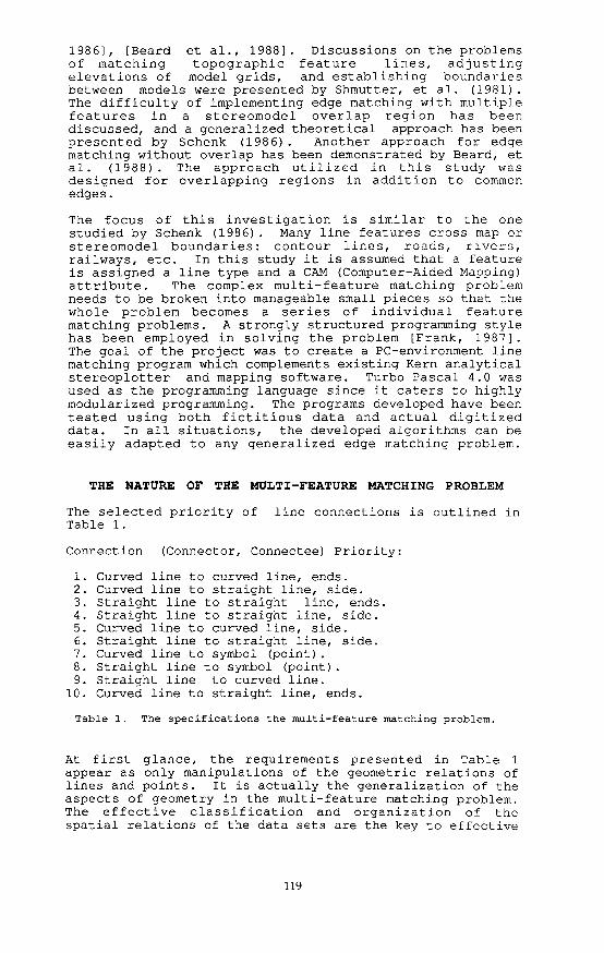
THE NATURE OF THE MULTI-FEATURE MATCHING PROBLEM

The selected priority of line connections is outlined in Table 1.

Connection (Connector, Connectee) Priority:

1. Curved line to curved line, ends.2. Curved line to straight line, side.3. Straight line to straight line, ends.4. Straight line to straight line, side.5. Curved line to curved line, side.6. Straight line to straight line, side.7. Curved line to symbol (point).8. Straight line to symbol (point).9. Straight line to curved line.

10. Curved line to straight line, ends.

Table 1. The specifications the multi-feature matching problem.

At first glance, the requirements presented in Table 1 appear as only manipulations of the geometric relations of lines and points. It is actually the generalization of the aspects of geometry in the multi-feature matching problem. The effective classification and organization of the spatial relations of the data sets are the key to effective

119

management of a large amount of digital information.

The specifications in Table 1 can be generally divided into two distinct categories. Certain situation occurs only in the overlapping region of two data sets. This situation is restricted to the same line types in both data sets as in the first and third rows in Table 1. The second situation is generalized line matching of any map information. This paper addresses the later situation as a stretch/peelback ("clean" line connection) problem, and it should not be mixed with the first line matching problem. The two problems are thus addressed separately.

While a line type is straight, curved, or a symbol, the CAM mode describes the line by color, thickness, and nature (dotted, dashed, etc). Essentially only one line matching algorithm has been developed as straight lines and symbols are treated as special types of curved lines.

GENERAL SCHEME OF THE PROGRAM STRUCTURES

Two programs have been developed to solve the identified problems of line matching in an overlapping region (MODTIE) and the stretch/peelback problem (PRETIE). PRETIE can be implemented before or after implementing the edge matching program MODTIE. Since both programs handle the same geometric entities, many of the same modularized routines can be used in each. Both programs use the same format for an input connection file. An example is listed in Table 2.

CONNECTOR________CQNNECTEE_________TOLERANCE______CONDITIONL2, ClL2, ClL2, ClL5, C2LI, Cl

L2,L2,L2,L5,LI,

ClClClC2Cl

55532

CESMM

Table 2. Example of a connection file.

In Table 2 L# is the line type number and C# is the CAM mode number. This constitutes a unique identifier for an individual line type. The programs decide which connection needs to be implemented based on the connection condition. In these conditions, S means end to side, C is self-closed, and E is an end to end connection. These conditions are resolved in PRETIE. M indicates edge matching, and is thus resolved in MODTIE.

The mechanism of program MODTIE will be described in detail in the following sections. Since program PRETIE has many similarities, a discussion of it will be generalized.

While program PRETIE operates on data in a single input file, program MODTIE operates on two input data files and creates one output file. MODTIE needs to manipulate the data only within the overlapping region of the two data sets. In photogrammetric model joins this region is relatively small since at the usual 60% overlap between

120

photos there is only a 10% overlap between the adjacent models. The data outside the overlap region does not need to be analyzed. The overlapping region, called a user-box, can be defined by the software automatically, or by user definition. Figure 1 represents the data separation idea, where Mapl and Map2 are the input data files, and Map3 is the output data file.

After the data in the overlapping region have been separated from the original data files, they are stored in temporary files. The software then utilizes individual line and CAM types for single feature matching in the fashion illustrated in Figure 2.

FORM OVERLAP REGION (USER-BOX)

A LINE HAVE THE REQUIRED

LINE TYPE?

Figure 1. Data separation and analysis.

121

OVERLAP REGION

DATA FROM MAPI

\ r

TEMPI

OVERLAP REGION DATA FROM MAP 2

1TEMP2

SELECT A LINE TYPE & CAM MODE

PUT TEMPI'S SELECTED L#C# IN Tl

PUT TEMP2'S SELECTED L#C# -IN T2

DELETE THE L#C# FROM TEMP1&TEMP2

PLACE REMAINING DATA IN T1/T2 IN MAP3

Figure 2. Break down the multi-feature problem into

single feature problems.

122

The general structure of program PRETIE is illustrated in Figure 3.

IMPLEMENTATIONS

Identification of Conjugate Lines

The unique identifier L#C# (line type and CAM mode) allows software to concentrate on the same feature from two groups. Ideally, each line in one file, should have a corresponding line in the other file. If it is not true, there is a "dead end" to the line in the overlap region. Either this is a mistake or an actual occurrence. This situation is alerted to the operator.

To locate a pair of lines that appears suitable for connection, a search for an intersection of the two lines is conducted. Non-intersecting lines are connected if the minimum distance between them does not exceed the user- specified tolerance. A rectangle search region about the lines is created by the software (Figure 4) . In addition to the distance checking, information such as elevation associated with contour lines is used to ensure a high percentage of correct identifications.

This method is successful if a user defines reasonable tolerance limits on line matches. These tolerances must be based on the quality of the data.

Based on the identification of conjugate lines, the connection between the lines is then conducted. A line can have multiple connections in the overlapping region (Figure 5) . This situation further complicates the connection algorithm. To ensure a high percentage of successful connections, a general algorithm has been developed which efficiently continues to look for additional connections to the conjugate line.

A final problem which had to be resolved in connecting overlapping lines is which portion of a particular line needs to be discarded. All examples in figure 6 represent a curved line which needs to be connected, and it is obvious the connected line should pass through both the left and right ends of the overlap region. The direction of a line is arbitrary and the line connection algorithm has been developed to handle all four situations. The algorithm consists of two steps. The first step of the algorithm ensures that the two lines are merged along the original direction of the first line. The second step of the algorithm solves the ambiguity problem resulting fromthe four situations in Figure 6. The resolved ambiguity is represented in Figure 7 where Figure 7(a) results from 6 (a) and 6(b), and 7(b) from the 6(c) and 6(d). The algorithm inverts the direction of the first line and conducts the line connection again. By comparing the length of the two connected lines, the longer one is selected as the final result.

123

SEPARATE THE INPUT DATA FILE

STRAIGHT

LINESSYMBOLS OTHERS

IMORE DEFINED CONNECTIONS?

IREAD IN A CONNECTOR/CONNECTEE

EXTRACT CONNECTOR DATA

FROM APPROPRIATE FILE

EXTRACT CONNECTEE DATA

FROM APPROPRIATE FILE

PERFORM STRETCH/PEELBACK ON THIS DATA

PLACE CONNECTOR DATA

BACK IN APPROPRIATE

FILE

PLACE CONNECTEE DATA

BACK IN APPROPRIATE

FILE

PUT ALL DATA INTO OUTPUT FILE

Figure^ 3. General flowchart of program PRETIE.

124

Figure 4. Rectangle search region for line match.

Data I Data

Figure 5. Multiple line matches.

start

start

start

start

end

end

end(O

start

end

Figure 6. Four situations of the relative relationship between two conjugate lines.

125

start

start (a) (b)

Figure 7. Two possible results after connecting the lines of Figure 6.

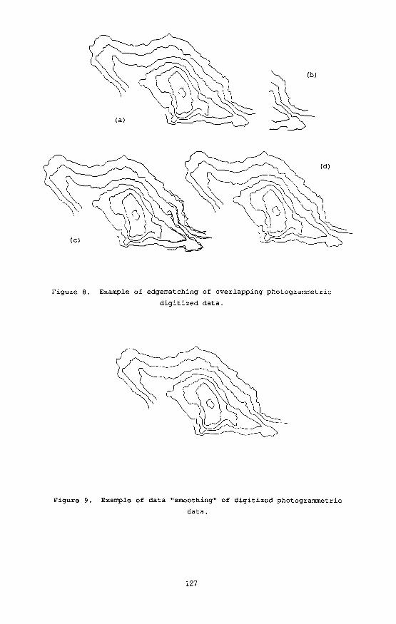
Figure 8 demonstrates an example of matching digitized contours, where 8(a) and 8(b) are the results from two adjacent photogrammetric stereomodels, 8(c) is the combination of 8(a) and 8(b) without processing, and 8 (d) is the merged results after running program MODTIE.

From Figure 8 it can be seen that there are some disconnections among the contours in the model. This is a special situation of stretch/peelback. The "smoothed" result using program PRETIE is illustrated in Figure 9.

CONCLUSIONS

A structured approach in solving the edge matching problem has been shown to be successful. The key in this approach is to break down a large and complex problem into many small ones that are manageable. With this approach a high percentage of line matching and stretch/peelback connections can be fully automated.

ACKNOWLEDGEMENTS

The authors wish to thank Kern Instruments, Inc., of Brewster, New York for their support in this research.

REFERENCES

Beard, K.M., 1988, A Localized Approach to Edgematching, The America Cartographer r Vol. 15, No. 2, pp. 163-172.

Frank, A.U., 1987, Geometry and Computer Graphics, Class Notes, Dept. of Surveying Engineering, University of Maine, Orono, Maine.

Schenk, T., 1986, A Robust Solution to the line-Matching Problem in Photogrammetry and Cartography, Photogrammetric Engineering and Remote Sensing r Vol. 52, No. 11, pp. 1779- 1784.

Shmutter, B., and Y. Doytsher, 1981, Matching Between Photogrammetric Models, The Canadian Surveyor, Vol. 35, No. 2, pp. 109-119.

126

(a)

(d)

(c)

Figure 8. Example of edgematching of overlapping photogrammetric

digitized data.

Figure 9. Example of data "smoothing" of digitized photogrammetric

data.

127