Embed Size (px)
Citation preview
Copyright © SEL 2016
Traveling Waves ForFault Location and Protection
Venkat Mynam
Copyright © SEL 2016

Source-Free Wave Equation…Free Space
0
0
2
0 0 2
22
2 2
B HxEt t
D ExHt t
Ex xEt
1 EE 0c t
0 0
1c

On a Lossless Line
Solutions are any function of the form:
2 2
2 2 2V 1 V 0
x c t

Propagation Along a Line
• Forward (Left) and backward (right) traveling waves maintain their shape if there are no losses, until they “hit” something
• Losses cause traveling waves to attenuate and usually distort…
…unless R GL C

Propagation Along a Line
• Skin effect vs frequencyincreases R, decreases L
• Corona can far exceed I2R losses
• Ground mode is more resistive

Discontinuities: Faults, Buses, …
At the discontinuity,
ρV, Reflection Coefficient
I RD
I R
D CR I
D C
C DR I
C D
v vv Zi i i
1 shortZ Zv vZ Z 1 open
1 shortZ Zi iZ Z 1 open


Out on the Power Line(The birth of a traveling wave)
GROUND
t
408 kVVoltage Collapse
InsulatorSportsman
Zot!!

At the Instant of Voltage Collapse
• A traveling 408 kV wave front emanates in both directions on the faulted conductor
• Current waves are con”currently*” producedvF
iF
vFiF
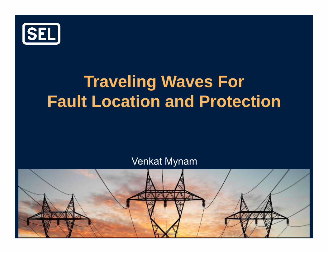
As the voltage/current Wave Front Travels
X
• Rise time increases• Amplitude decreases
e
High frequencies attenuated due to conductor skin effect losses

Faults Launch Traveling Waves

No Detectable High-Frequency Transient at Line Terminal When Fault
Inception Angle Is Zero

Am
pere
s
TW Fault Location PrincipleSingle End and Double End

BPA and BC Hydro Successfully Used This Technology to Locate
Faults

Accurately Locate Faults With Traveling Waves
For a fault at 38.16 miles
Method Distance (miles) Difference (miles)
Impedance 34.03 4.13
Traveling wave (TW) 37.98 0.18

CT Bandwidth Is Adequate to Capture TWs
R. C. Dugan, M. F. McGranaghan, and H. W. Beaty, Electrical Power Systems Quality. McGraw Hill, New York, NY, 1995.

CVTs Have Limited Bandwidth
M. Kezunovic, L. Kojovic, V. Skendzic, C. W. Fromen, D. R. Sevcik, and S. L. Nilsson, “Digital Models of Coupling Capacitor Voltage Transformers for Protective Relay Transient Studies,” IEEE Transactions on Power Delivery, Vol. 7, Issue 4, October 1992, pp. 1927–1935.

• Forming vI, vR uses all the information (v and i) helps sort out reflected, transmitted waves
• CTs are pretty “hi-fi” for transients: over 100 kHz
• CCVTs are not, except at the capacitive voltage divider tap, but that means new cabling
• Use currents and two-end method
• Perfect in current differential relays
• Reuse same communications channel
Practical Considerations

• Availability of TWFL for all lines
• No need for new wires or sensors
• Built-in relay-to-relay communication
• Built-in time synchronization
• Protection elements to aid fault location
• Z-based fault locator that complements TWFL
Advantages of TWFL in Relays

• Filter and sample phase currents
• Isolate desired aerial mode
• Accurately measure time of arrival
• Exchange arrival time with other end, over same 87L channel
• Calculate location using two-ended TWFL equation
TW Fault Locator Design

Differentiator-Smoother Works GreatBorrowed Idea From “Leading-Edge
Tracking”
Interpolate to50 ns Accuracy
s
a
s
s
Current Arrival Timei(t) is(t)
tadis/dt

Relative Accuracy ~ 50 ns
Mean Error = 17 ns or 8′
Standard Deviation = 32 ns or 16′

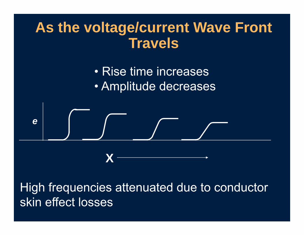
First Application Helps Locate Faults on Challenging 161 kV Line
SEL-411LSEL-411L
SEL-411L Reported Ground Fault at 59.04 Miles

“We Know Where Your Faults Are”
Nature of Fault Line Patrol (miles) TW (miles)
Flashover 67.91 68.19
Lead projectile 38.16 37.98
Lightning 66.86 67.25
Flashover 61.50 61.42
Flashover 50.18 50.56
Flashover 59.04 59.04
Accuracy within one to two tower spans

SEL-411L TW Works on Tapped Lines115 kV, 112.85-Mile Line

Line Energization From Brasada Identifies Tap Locations
Am
pere
s

Line Patrol – It Was Like “Chasing Ghosts on This Line”
Nature of Fault Line Patrol (miles) TW (miles)
Flashover 36.65 36.33
Flashover 36.65 36.76
Flashover 6.92 6.92*
Flashover 91.62 91.76
Flashover 4.94 4.94*
Bird waste 47.1 47.35
*Single-ended fault location
Accuracy within one to two tower spans

Single-Ended TWFLChallenging to Identify Correct Reflections
First Wave
Reflection 1Reflection 2

Impedance-Based Fault Location Sorts Reflections
Calculates FL at 6.95 MilesBrasada Terminal Open
Ideal Condition for Impedance FL

Impedance Points Way, TW Finds Fault Calculated at 6.92 Miles
First Wave
Reflection From Fault

TW Fault Location Is Perfect for Series-Compensated Lines

Estimate Propagation Velocity and Fault Location
First Wave
Reflection From FaultReflection From Remote Terminal
fault remote
2 •LLVelocity = = 0.98069(∆t +∆t ) • c

CFE Reported 55.67 Miles for This Fault
SEL-411L TW (miles) Standalone TW (miles)
55.66 55.43

SEL-411L Relays With TW Function In Service on 345 kV Underground Cables

Waves Propagate Slower in Underground Cables
Wave Velocity = 0.48 Times Speed of Light
Event captured during cable energization

Locate Temporary and Permanent Faults Using Traveling Waves

TW Technology for Protection of Transmission Lines

15 MW more per millisecond savedR. B. Eastvedt, BPA, 1976 WPRC
The Need for SpeedMoving Energy at the Speed of Light
Safer • Less Damage • Improved Dynamics

Why Today? The Need for Speed
Faster communicationsPowerful processors
Better simulationsMay be simpler
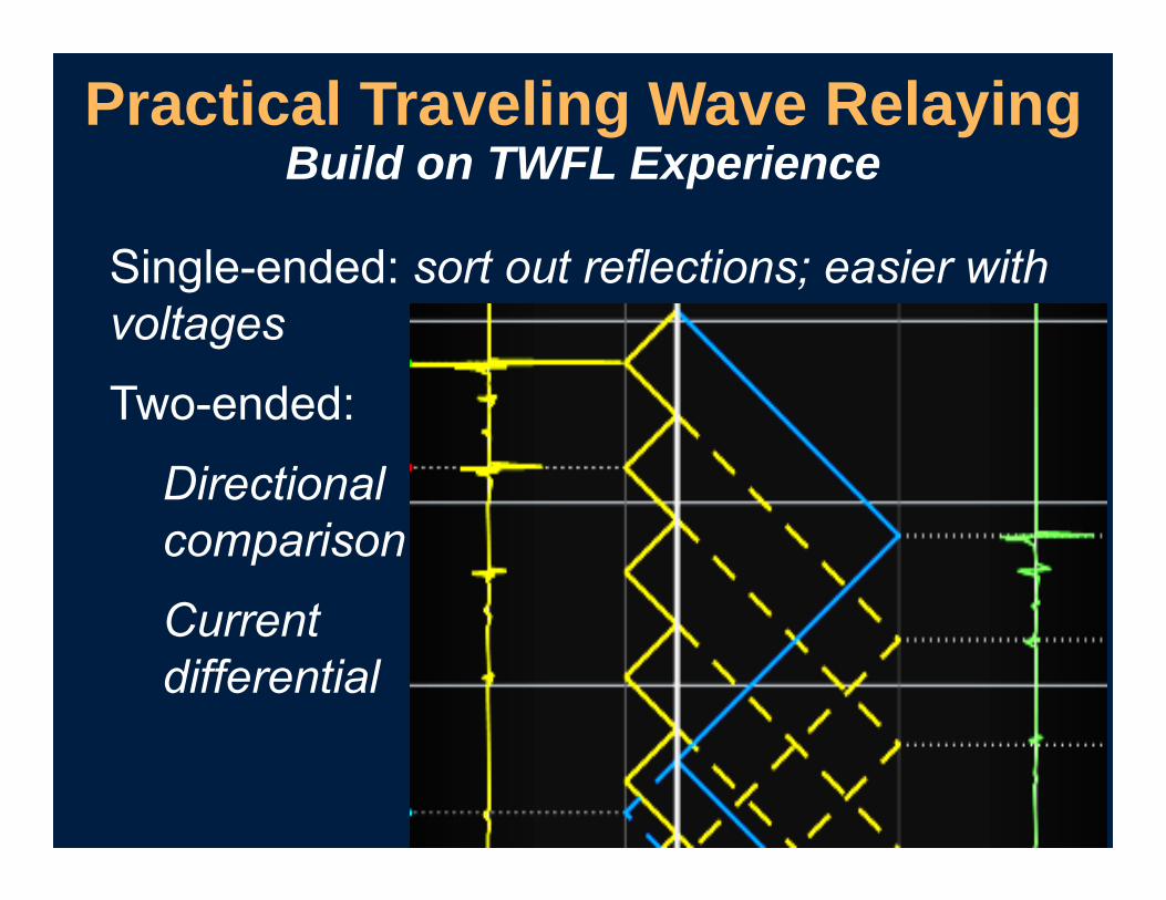
Practical Traveling Wave RelayingBuild on TWFL Experience
Single-ended: sort out reflections; easier with voltages
Two-ended:
Directional comparison
Current differential

Speed of Light Limits Relay Time
The fastest communications path is the line
S R100-mile line ≈ 600 µs X
300 μs 300 μs
600 μs by line or 1,000 μs by fiber
900 μs or 1,300 μs

TW Directional Element Principle
vTW iTW
+–
–+ Forward
+–
+– Reverse
vTW
iTW
iFvTW iTW vF
vF

TW32F Asserts – Forward Fault
TW32F Operate

0 100 200 300 400 500-100
0
100
Time (µs)600
-5
0
5
0 100 200-50
0
50
Time (µs)300 400 500 600
-2
0
2
0 100 200 300 400 500 600-1000
-500
0
Time (µs)
TW32R Asserts – Reverse Fault
TW32R Operate

TW32F Asserts if vTW and iTW Are Opposite in Polarity

New TW Differential PrincipleCurrent Only
• Internal fault surges: same polarity• External fault surges: Generally of opposite polarity
Spaced one travel time T apart
Σ of aligned surges = OPERATE
∆ of surges T apart = RESTRAIN

Internal Mid-Line Fault
S R
IF(0)
Σ = Is(300) + Ir(300) = BIG∆ = Is(300) − Ir(300 +/− 600) = small
IF(0)
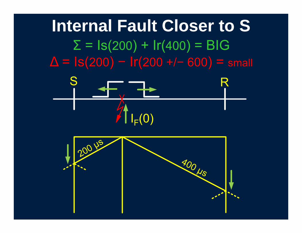
Internal Fault Closer to SΣ = Is(200) + Ir(400) = BIG
∆ = Is(200) − Ir(200 +/− 600) = small
S R

TW87 Principle – Internal Fault
Line propagation time
m87 < 1 pu

S
IF(0)
External Fault Travels the Entire LineΣ = Is(50) + Ir(650) = small
∆ = Is(50) − Ir(50 +/− 600) = BIGR

TW87 Principle – External Fault
Line propagation time
m87 = 1 pu
Loca
l Cur
rent
(A)
Rem
ote
Cur
rent
(A)
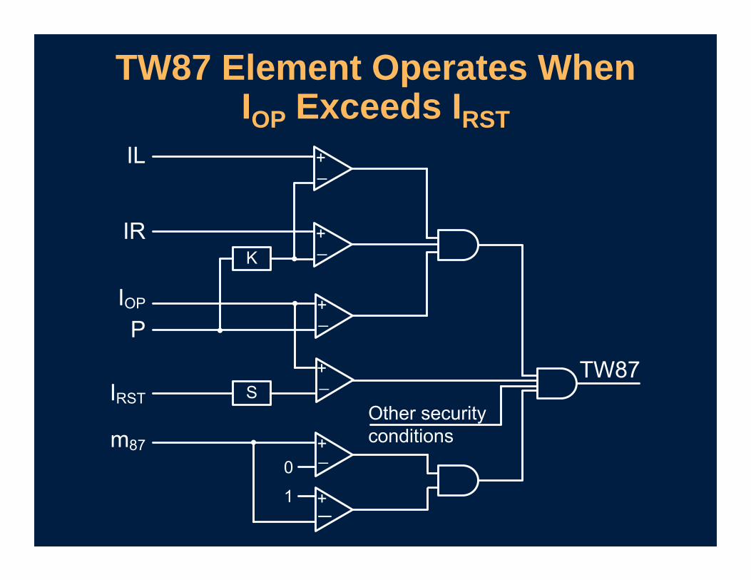
TW87 Element Operates When IOP Exceeds IRST
OP
RST
87

TW87 Performance: 161 kV,117 km LineBG Fault, 117 km, Fault is at 18%
Pha
se A
TW (A
)P
hase
BTW
(A)
Pha
se C
TW (A
)
IL = 0.68 AIR = 0.35 AIOP = 1.03 AIRST = 0.13 Am87 = 0.81 pu
TT=396 s

F F
Trip in 1.2 ms
Time (µs)
321
972
TW87 Operating Time on a 117 km Line
75

Traveling Waves Provide Accurate Fault Location and High Speed Line Protection