Embed Size (px)
Citation preview

TREATABILITY OF EMERGING CONTAMINANTS IN WASTEWATER
TREATMENT PLANTS DURING WET WEATHER FLOWS
by
KENYA L. GOODSON
ROBERT E. PITT, COMMITTEE CHAIR
STEVEN DURRANS
DEREK WILLIAMSON SAM SUBRAMANIAM
SHIRLEY CLARK
A DISSERTATION
Submitted in partial fulfillment of the requirements for the degree of Doctor of Philosophy
in the Department of Civil, Construction and Environmental Engineering in the Graduate School of
The University of Alabama
TUSCALOOSA, AL
2013

Copyright Kenya L. Goodson 2013 ALL RIGHTS RESERVED
ABSTRACT
Municipal wastewater treatment plants have traditionally been designed to treat conventional
pollutants found in sanitary wastewaters. However, many synthetic pollutants, such as
pharmaceuticals and personal care products (PPCPs), also enter the wastewater stream. Some of
these nontraditional contaminants are not efficiently removed by the treatment process at the
wastewater treatment plant. Emerging contaminants (ECs) have been identified in surface
waters receiving wastewater effluents and have been found to potentially cause adverse effects
on aquatic wildlife. These materials are produced by industry in very large quantities and are
disposed of in toilets and in industrial effluent where partial treatment occurs before their
discharge. Some of the pharmaceuticals excreted from the human user’s body are metabolized
and are more toxic and untreatable than their parent compound. Emerging contaminants have
been referred to by EPA as “contaminants of emerging concern (CECs) because the risk to
human health and the environment associated with their presence, frequency of occurrence, or
source may not be known.”
In this EPA funded research, pharmaceuticals, PAHs and pesticides at the treatment
plants were examined. The study focuses on the effects of stormwater infiltration, the inflow
into sanitary systems and the amounts and treatability of targeted pharmaceuticals. Stormwater is
a known source of many contaminants and could mix with wastewater through stormwater
infiltration and inflow (I & I). Several dry and wet weather series of samples were obtained from
the city of Tuscaloosa’s wastewater treatment plant. Samples were examined from four locations
within the treatment plant in order to determine if there are significant differences between
influent quantities and removal characteristics during periods of increased flows associated with
ii

wet weather compared to normal flow periods. The data generally show treatability appears to
remain similar during both wet and dry weather conditions under a wide range of flow
conditions. Changes in hydraulic retention times and hourly flow variations were also observed
to determine treatment plant performance.
Emphasis was placed on the following pesticides: aldrin, chlordane, dieldrin, endrin,
gamma-BHC, heptachlor, heptachlor epoxide, hexachlorobenzene, hexachlorocyclopentadiene,
methoxychlor, and toxaphene. As expected, not all compounds were quantified in the samples,
with many being below the detection limits.
iii

DEDICATION
This dissertation is dedicated to the generations before me who did not have the resources or
opportunity to receive a post-secondary education. I want to particularly dedicate this work to
my grandmother, Martha Goodson, who worked in housekeeping for over 15 years at the
University of Alabama.
iv

LIST OF ABBREVIATIONS
PCBs- polycyclic biphenyls (Arochlor)
CBZ-carbamazepine
CSOs-Combined sewer overflows
CAS-conventional activated sludge
ECs-Emerging contaminants
ECOC-Emerging contaminants of concern
EDCs endocrine disruptor compounds
FLX-fluoxetine
GFB-Gemfibrozil
HMW-High molecular weight
HRT-hydraulic retention time
IBP-Ibuprofen
LMW-Low molecular weight
MBR-membrane bioreactor
OCP-Organochlorine Pesticides
PPs-Pharmaceutical products
PhACs-Pharmaceutically Active Compounds
PPCPs-Pharmaceuticals and personal care products
PAHs-polyaromatic hydrocarbons
PEs-population equivalents
v

POP-Persistent Organic Pollutant
STPs- Sewage treatment plants
SRT-solids retention time
SMZ-sulfamethoxazole
TCL-Triclosan
TRM-trimethoprim
WWTP-Wastewater treatment plant
BQ-Below quantification
BDL-Below detection limit
MDL-Method Detection limit
vi

ACKNOWLEDGEMENTS
I am thankful for what I believe was a divine journey. There were several individuals
who assisted me through this process. I would like to thank the Department of Civil,
Construction and Environmental Engineering for giving me the opportunity to obtain a PhD. Dr.
Pauline Johnson was instrumental in my acceptance and I appreciate that tremendously. I also
want to thank my advisor and dissertation chair, Dr. Robert Pitt. I am appreciative to him for
giving me the opportunity to work with him on the EPA project. Through him, I have learned
about patience, perseverance and having a passion for scholarly work. Thank you for being so
patient and understanding with me through this process. I would not have finished this process if
it were not for your diligence and quick thinking when several roadblocks came my way. I would
also like to thank all my committee members for your thoughtful insight and recommendations to
make my dissertation a better scholarly work. I would like to thank two of my committee
members in particular for the analysis of my data: Dr. Sam Subramaniam from Miles College
and Dr. Shirley Clark from Penn State Harrisburg. Thank you to the Environmental Protection
Agency and the National Science Foundation (EPSCoR) for the funding received to complete
this project. I thank my colleagues, Redi, Olga, Leila and Brad for their insight and
encouragement through my journey. John Harden was also a great encouragement to me. You
are more than a colleague: you are a great friend!
When obtaining my PhD, it was important for me to have a support system. Without
these individuals, I would have given up the journey. I would like to thank my friends who I met
through the African-American Graduate Student Association for encouraging me when things
got really difficult. Ebony Johnson and Nadia Richardson were two of my closest friends who
walked with me through my ups and downs. They also obtained their PhDs through rough waters
vii

and have encouraged me to do the same. I would like to thank Kathy Echols, BJ Guenther and
the Women’s Dissertation Support group for their love, support and encouragement when all I
wanted to do was procrastinate. Accountability is important in this process.
I would like to thank my chair, Dr. Robert Pitt; the department chair, Dr. Ken Fridley and
Dr. John Schmitt from the Graduate School for helping me through the challenges that I faced
toward the end of my matriculation. I would not be finished if it were not for you.
Lastly, I would like to thank my family for their prayers, support and encouragement then
I had many doubts and fears. Mom, thanks for supporting me at my defense! Marilyn, thank you
for your help! I love you guys tremendously! I offer a VERY special thank you to Angela
Mitchell! She provoked me with a strong tongue to stop talking about graduate school and DO
IT! I would not be a PhD if it were not for you!
viii

CONTENTS
ABSTRACT .................................................................................................................................... ii
DEDICATION ............................................................................................................................... iv
LIST OF ABBREVIATIONS ..........................................................................................................v
ACKNOWLEDGEMENTS .......................................................................................................... vii
CONTENTS ................................................................................................................................... ix
LIST OF TABLES ......................................................................................................................... xi
LIST OF FIGURES ..................................................................................................................... xiv
1.0 INTRODUCTION .....................................................................................................................1
1.1 OBJECTIVES ............................................................................................................................4
1.2 RESEARCH QUESTIONS .......................................................................................................5
2.0 LITERATURE REVIEW ..........................................................................................................6
2.1 TREATMENT AND PHYSICO-CHEMICAL PROPERTIES OF EMERGING CONTAMINANTS..........................................................................................................................7
2.1.1 Pharmaceuticals and Personal Care Products (PPCPS) ..............................................8
2.1.2 Polycyclic Aromatic Hydrocarbons ..........................................................................18
2.1.3 Pesticides and Herbicides .........................................................................................22
2.1.4 Endocrine Disruptors ................................................................................................27
2.2 WASTEWATER TREATABILITY IN CONVENTIONAL WWTP .....................................30
2.2.1 Description of Wastewater Unit Processes ...............................................................30
2.2.2 Wastewater Treatment of Emerging Contaminants as reported in the Literature ....33
2.2.2.1. Pharmaceuticals ..........................................................................................34
2.3 COMBINED SEWER SYSTEMS ...........................................................................................46
2.4 FINDINGS FROM THE LITERATURE AND NEED FOR RESEARCH ............................53
2.5 SUMMARY OF LITERATURE REVIEW.............................................................................55
ix

3.0 METHODOLOGY ..................................................................................................................60
3.1 HYPOTHESES ........................................................................................................................61
3.2 SITE LOCATION ....................................................................................................................61
3.2.1 General Characteristics .............................................................................................61
3.2.2 Description of the Unit Processes .............................................................................62
3.2.3 Drainage around the Treatment Plant .......................................................................65
3.2.4 Industrial Influent......................................................................................................67
3.2.5 Performance Parameters at Tuscaloosa WWTP .......................................................68
3.3 EXPERIMENTAL DESIGN ...................................................................................................76
3.4 DATA ANALYSES.................................................................................................................80
3.4.1. Descriptive Statistics ................................................................................................80
3.4.1.1. Statistical Tests .....................................................................................................80
3.4.1.2. Critical Tests .........................................................................................................81
4.0 RESULTS ................................................................................................................................83
5.0 CONCLUSIONS.............................………………………………………………………….94
6.0 LIMITATIONS ......................................................................................................................102
REFERENCES ............................................................................................................................105
APPENDIX A: DETAILED OBSERVATIONS ........................................................................113
APPENDIX B: CHROMATOGRAPHS FOR SAMPLE ANALYSES ......................................195
APPENDIX C: QUALITY ASSURANCE AND QUALITY CONTROL DATA .....................229
x

LIST OF TABLES
2.1. Selected Chemical Properties of Pharmaceuticals ..................................................................10
2.2. Log of octanol-water coefficients for carbamazepine and its metabolites .............................15
2.3. Characteristics of PAHs ..........................................................................................................20
2.4. Properties of Pesticides ...........................................................................................................24
2.5. Physical and Chemical Properties of Aroclors .......................................................................27
2.6. Properties of Endocrine Disruption Chemicals.......................................................................29
2.7. Reduction rates of ECs by primary sedimentation treatment .................................................35
2.8. EC reduction rates during secondary treatment (%) ...............................................................36
2.9. Characteristics of wastewater treatment plants .......................................................................37
2.10. Summary of EC Loads and Removal Rates at Wastewater Treatment Facilities .................38
2.11. Dissociation Constants, Influent and Effluent Concentrations of ECs .................................38
2.12. Influent and Effluent Concentrations, Detection Limits and Percent Reductions ................39
2.13. Percent reductions of ECs at conventional activated sludge wastewater treatment facilities
........................................................................................................................................................40
2.14. Comparison of Influent and Effluent and Percentage Reductions for ECs ..........................41
2.15. Comparison of Membrane Bio Reactor and Conventional Activated Sludge ......................43
2.16. Estrogen Influent and Effluent Concentrations .....................................................................44
2.17. PAH Categories ....................................................................................................................47
2.18. Mean, Standard Deviations and Removal Percentages of Influent and Effluent ..................50
2.19. PAH Concentrations through each unit process ...................................................................51
2.20a. Summary of Characteristics and Treatability of Targeted Pollutants .................................57
xi

2.20b. Summary of Characteristics and Treatability of Targeted Pollutants .................................58
3.1. Average and maximum flow rates from NPDES ....................................................................65
3.2. List of Industrial Sites that Discharge to the Hilliard N Fletcher Treatment Plant ........................................................................................................................................................68 3.3. Flow rates by rainfall categories during days of sampling .....................................................73
4.1 Treatment Plant Average Daily Flow Rates and Daily Total Rain Depth on Days of Sampling ........................................................................................................................................................84 4.2. Estimated Stormwater Infiltration and Inflow (I&I) for Different Rain Categories ...............88
4.3. Influent Mass Load Data for Pharmaceuticals during Dry Weather .......................................88
4.4. Influent Mass Load Data for Pharmaceuticals during Wet Weather ......................................88
4.5. Performance Data for Earl Hilliard WWTP ............................................................................90
4.6. Preliminary semivolatile analyses results (phthalate esters and pesticides) ...........................92
5.1. Summary Statistical Test Results for Selected ECs Examined during this Research ...........104
A.1.1. Summary Data for Gemfibrozil ...................................................................................... .113
A.1.2. Summary Data for Ibuprofen .......................................................................................... .120
A.1.3. Summary Data for Triclosan ........................................................................................... .126
A.1.4. Summary Data for Carbamazepine ................................................................................. .133
A.1.5. Summary Data for Fluoxetine ......................................................................................... .138
A.1.6. Summary Data for Sulfamethoxazole ............................................................................. .143
A.1.7. Summary Data for Trimethoprim ................................................................................... .148
A.2.1. Summary Data for Naphthalene ...................................................................................... .152
A.2.2. Summary Data for Acenaphthene ................................................................................... .159
A.2.3. Summary Data for Fluorene ............................................................................................ .164
A.2.4. Summary Data for Fluoranthene ..................................................................................... .169
A.2.5. Summary Data for Acenaphthylene ................................................................................ .174
A.2.6. Summary Data for Phenanthrene .................................................................................... .179
xii

A.2.7. Summary Data for Anthracene ....................................................................................... .184
A.2.8. Summary Data for Pyrene ............................................................................................... .189
C.1. Pesticide and PAH detection limits (from PSH Analysis) ...................................................245
xiii
LIST OF FIGURES
2.1. Comparison of dry and wet weather concentrations for total PAHs ......................................48
2.2 Concentrations of pesticides ....................................................................................................52
2.3. Concentration of ƩPCBs .........................................................................................................53
3.1. Schematic of Hilliard N. Fletcher WWTP ..............................................................................64
3.2. Topographic map from NPDES permit ..................................................................................66
3.3a. Tuscaloosa Treatment plant CBOD influent and effluent data from 2005-2008 ..................69
3.3b. Tuscaloosa Treatment plant TSS influent and effluent data from 2005-2008 ......................70
3.4. Scatterplots of TSS concentrations vs. daily rain depths ........................................................70
3.5. Scatterplots of CBOD concentrations vs. daily rain depths ....................................................70
3.6. Comparison of rainfall and flow rates ....................................................................................71
3.7: Boxplots showing rainfall vs. flows for 2010-2012 ...............................................................72
3.8. Box and Whisker plot for sampling events .............................................................................73
3.9. Primary clarifier hydraulic resident time (HRT) during days of sampling for the Hilliard N. Fletcher WWTP .............................................................................................................................74
3.10. Graph of HRT for aeration basin during days of sampling for the Hilliard N. Fletcher WWTP ...........................................................................................................................................75
3.11. Graph of HRT for secondary clarifiers during days of sampling for the Hilliard N. Fletcher WWTP ...........................................................................................................................................76
4.1. Treatment plant flows during dry and wet weather ................................................................86
4.2. Treatment plant flow compared to rain total ...........................................................................87
4.3. Triclosan influent concentrations vs. treatment plant flow rates ............................................89
4.4. Treatability line plot for naphthalene during dry weather ......................................................91
5.1. EC concentrations vs. treatment plant flow rate ...................................................................102
A.1.1.1 Probability plot for Gemfibrozil .....................................................................................114
A.1.1.2 Line graph of Gemfibrozil at four sampling locations ....................................................115
xiv

A.1.1.3 Box and Whisker plots for Gemfibrozil ..........................................................................116
A.1.2.1. Probability plots for Ibuprofen .......................................................................................121
A.1.2.2. Line graphs for Ibuprofen at four sampling locations ....................................................122
A.1.2.3 Box and Whisker plots for Ibuprofen .............................................................................123
A.1.3.1 Probability plots of Triclosan at four sampling locations ...............................................127
A.1.3.2 .Graph of Triclosan during Dry Weather ........................................................................128
A.1.3.3. Line plots of Triclosan at four sampling locations ........................................................129
A.1.3.4. Box and Whisker Plot for Triclosan ..............................................................................130
A.1.4.1. Probability Plot for Carbamazepine ...............................................................................134
A.1.4.2 Line plot for Carbamazepine at four sampling locations ................................................135
A.1.4.3. Box and Whisker Plots for Carbamazepine ...................................................................136
A.1.5.1. Probability plot for Fluoxetine .......................................................................................139
A.1.5.2 Line graph of Fluoxetine at four different sampling locations .......................................140
A.1.5.3 Box and Whisker Plots for Fluoxetine ............................................................................141
A.1.6.1 Probability Plot for Sulfamethoxazole ............................................................................144
A.1.6.2 Line graph for Sulfamethoxazole at different sampling locations ..................................145
A.1.6.3. Box and Whisker Plots for Sulfamethoxazole ...............................................................146
A.1.7.1 Probability Plot for Trimethoprim ..................................................................................149
A.1.7.2 Line graph for Trimethoprim at different sampling locations ........................................149
A.1.7.2 Box and Whisker Plots for Trimethoprim.......................................................................150
A.2.1.1. Probability plots for Naphthalene ..................................................................................153
A.2.1.2.Graph of Naphthalene during Wet Weather ...................................................................154
A.2.1.3. Graph of Naphthalene during Dry Weather ...................................................................155
A.2.1.4. Line graph for Naphthalene (total) at four sampling locations ......................................156
A.2.1.5. Box and Whisker plot for Naphthalene..........................................................................157
xv
A.2.2.1. Probability Plot for Acenaphthene .................................................................................160
A.2.2.2 Line graph for Acenaphthene at four different sampling locations ................................161
A.2.2.3 Box and Whisker Plot for Acenaphthene ........................................................................162
A.2.3.1 Probability plot for Fluorene ...........................................................................................165
A.2.3.2. Line plot for Fluorene at four different sampling locations ...........................................166
A.2.3.3. Box and Whisker Plots for Flourene ..............................................................................167
A.2.4.1 Probability plots for Fluoranthene ..................................................................................170
A.2.4.2 Line graph for Fluoranthene at four different sampling locations ..................................171
A.2.4.3 Box and Whisker Plots for Fluoranthene ........................................................................172
A.2.5.1. Probability plot for Acenaphthylene ..............................................................................175
A.2.5.2. Line graph for Acenaphthylene at four different sampling locations ............................176
A.2.5.1. Box and Whisker Plots for Acenaphthylene ..................................................................177
A.2.6.1. Probability plot for Phenanthrene ..................................................................................180
A.2.6.2 Line graph for Phenanthrene at four different sampling locations .................................181
A.2.6.3. Box and Whisker Plots for Phenanthrene ......................................................................182
A.2.7.1 Probability Plot for Anthracene ......................................................................................185
A.2.7.2. Line graph for Anthracene at four different sampling locations ....................................186
A.2.7.3 Box and Whisker Plots for Anthracene...........................................................................187
A.2.8.1. Probability plots for Pyrene ...........................................................................................190
A.2.8.2 Line graphs for Pyrene at four different sampling locations ..........................................190
A.2.8.3. Box and Whisker Plots for Pyrene .................................................................................191
B.1. Influent Sample for 11/08/12: Acid Group I ........................................................................195
B.2. Influent Sample for 11/08/12: Acid Group II.......................................................................195
B.3. Primary Effluent Sample for 11/08/12: Acid Group I..........................................................196
B.4 .Primary Effluent Sample for 11/08/12: Acid Group II ........................................................196
xvi

B.5. Secondary Effluent Sample for 11/08/12: Acid Group I ......................................................197
B.6. Secondary Effluent Sample for 11/08/12: Acid Group II ....................................................197
B.7. Final Effluent Sample for 11/08/12: Acid Group I ..............................................................198
B.8. Final Effluent Sample for 11/08/12: Acid Group II .............................................................198
B.9. Final Spiked Effluent Sample for 11/08/12: Acid Group I ..................................................199
B.10. Influent Sample for 11/12/12: Acid Group I ......................................................................199
B.11. Influent for 11/12/12: Acid Group II ..................................................................................200
B.12. Primary Effluent for 11/12/12: Acid Group I.....................................................................200
B.13. Primary Effluent for 11/12/12: Acid Group II ...................................................................201
B.14. Secondary Effluent for 11/12/12: Acid Group I .................................................................201
B.15. Secondary Effluent from 11/12/12: Acid Group II ............................................................202
B.16. Final Effluent for 11/12/12: Acid Group I .........................................................................202
B.17. Final Effluent from 11/12/12: Acid Group II .....................................................................203
B.18. Final Effluent (Spiked) for 11/12/12: Acid Group I ..........................................................203
B.19. Primary Effluent from 05/11/11: Acid Group II ................................................................204
B.20. Influent from 03/02/10: Acid Group II ..............................................................................204
B.21. Primary Effluent from 03/02/10: Acidic Group II .............................................................205
B.22. Secondary Effluent from 03/02/10: Acid Group II ............................................................205
B.23. Final Effluent from 03/02/10: Acid Group II .....................................................................206
B.24. Influent from 06/25/10: Acid Group II ..............................................................................206
B.25. Primary Effluent from 06/25/10: Acid Group II ................................................................207
B.26. Secondary Effluent from 06/25/10: Acid Group II ............................................................207
B.27. Final Effluent from 06/25/10: Acid Group II .....................................................................208
B.28. Influent from 11/02/10: Acid Group II ..............................................................................208
B.29. Primary Effluent from 11/02/10: Acid Group II ................................................................209
xvii

B.30. Secondary Effluent from 11/02/10: Acid Group II ............................................................209
B.31. Final Effluent from 11/02/10: Acid Group II .....................................................................210
B.32. Influent from 03/09/11: Acid Group II ..............................................................................210
B.33. Primary Effluent from 03/09/11: Acid Group II ................................................................211
B.34. Secondary Effluent from 03/09/11: Acid Group II ............................................................211
B.35. Final Effluent from 03/09/11: Acid Group II .....................................................................212
B.36. Influent from 05/14/11: Acid Group II ..............................................................................212
B.37. Primary Effluent from 05/14/11: Acid Group II ................................................................213
B.38. Secondary Effluent from 05/14/11: Acid Group II ............................................................213
B.39. Final Effluent from 05/14/11: Acid Group II .....................................................................214
B.40. Influent from 09/20/11: Acid Group II ..............................................................................214
B.41. Primary Effluent from 09/20/11: Acid Group II ................................................................215
B.42. Secondary Effluent from 09/20/11: Acid Group II ............................................................215
B.43. Final Effluent from 09/20/11: Acid Group II .....................................................................216
B.44. Influent from 01/16/10: Acid Group II ..............................................................................216
B.45. Primary Effluent for 01/16/10: Acid Group II ...................................................................217
B.46. Secondary Effluent for 01/16/10: Acid Group II ...............................................................217
B.47. Final Effluent for 01/16/10: Acid Group II ........................................................................218
B.48. Influent from 03/20/11: Acid Group II ..............................................................................218
B.49. Primary Effluent from 03/20/11: Acid Group II ................................................................219
B.50 Secondary Effluent for 03/20/12: Acid Group II ................................................................219
B.51. Final Effluent for 03/20/12: Acid Group II ........................................................................220
B.52. Influent from 06/16/12: Acid Group II ..............................................................................220
B.53. Primary Effluent from 06/16/12: Acid Group II ................................................................221
B.54. Secondary Effluent from 06/16/12: Acid Group II ............................................................221
xviii

B.55. Final Effluent for 06/16/12: Acid Group II ........................................................................222
B.56. Influent from 09/15/12: Acid Group II ..............................................................................222
B.57. Primary Effluent from 09/15/12: Acid Group II ................................................................223
B.58. Secondary Effluent from 09/15/12: Acid Group II ............................................................223
B.59. Final Effluent from 09/15/12: Acid Group II .....................................................................224
B.60. Influent from 11/01/12: Acid Group II ..............................................................................224
B.61. Primary Effluent from 11/01/12: Acid Group II ................................................................225
B.62. Secondary Effluent from 11/01/12: Acid Group II ............................................................225
B.63. Final Effluent from 11/01/12: Acid Group II .....................................................................226
B.64. Influent from 11/04/12: Acid Group II ..............................................................................226
B.65. Primary Effluent from 11/04/12: Acid Group II ................................................................227
B.66. Secondary Effluent from 11/04/12: Acid Group II ............................................................227
B.67. Final Effluent from 11/04/12: Acid Group II .....................................................................228
C.1. Standard Curve for Naphthalene ..........................................................................................229
C.2. Standard Curve for Acenaphthylene ....................................................................................230
C.3. Standard Curve for Acenaphthene .......................................................................................231
C.4. Standard Curve for Fluorene ................................................................................................232
C.5. Standard Curve for Phenanthrene ........................................................................................233
C.6. Standard Curve for Anthracene ............................................................................................234
C.7. Standard Curve for Fluoranthene .........................................................................................235
C.8. Standard Curve for Pyrene ...................................................................................................236
C.9. Standard Curve for Chrysene ...............................................................................................237
C.10. Standard Curve for Ibuprofen ............................................................................................238
C.11. Standard Curve for Triclosan .............................................................................................239
C.12. Standard Curve for Gemfibrozil .........................................................................................240
xix

C.13. Standard Curve for Sulfamethoxazole ...............................................................................241
C.14. Standard Curve for Carbamazepine ...................................................................................242
C.15. Standard Curve for Fluoxetine ...........................................................................................243
xx

1.0 INTRODUCTION
The U.S. Environmental Protection Agency (EPA) sets guidelines for pollutant
discharges from municipal and industrial treatment plants and for stormwater discharges based
on the National Pollutant Discharge Elimination System (NPDES). These regulations mainly
focus on discharges of conventional pollutants. However, new classes of unregulated
contaminants have become an emerging environmental problem (Petrovic, Gonzalez, and
Barceló 2003, 685-696). These pollutants have recently been found in waterways and in
groundwater. Pharmaceuticals were first reported in surface waters during the investigation of
U.S. waterways in the 1970s, although they are not regulated as legacy pollutants such as PCBs
and DDTs (Snyder et al. 2006). Researchers such as Watts et al (1983) first reported the
occurrence of several selected antibiotics in river water samples. Since then, there have been
many investigations of antibiotics as well as publications documenting their presence in
groundwaters, surface waters, wastewaters and landfill leachates (Xu et al. 2007, 4526-4534).
The EPA works in conjunction with the U.S. Geological Survey to compile a list of these
contaminants found in the U.S. waterways (A National Reconnaissance). Samples have been
obtained from 139 U.S. streams and waterways to analyze ninety five organic wastewater
contaminants (Kolpin et al. 2002, 1202-1211). These emerging contaminants are employed in
large quantities during daily consumption. Yet many have no maximum concentration limits in
discharge permits. Research on several contaminants investigated during the Reconnaissance
Study is being conducted to decipher the potential effect of these compounds on aquatic wildlife
and the environment. Campbell (2006) conducted a study as an example to investigate the effects
of estrogen, an endocrine chemical disruptor, on aquatic wildlife.
1

Emerging contaminants as defined by the U.S. Geological Survey are “any synthetic or
naturally occurring chemical or any microorganism that is not commonly monitored in the
environment but has the potential to enter the environment and cause known or suspected
adverse ecological and (or) human health effects.” The U.S. EPA describes emerging
contaminants by the statement: “chemicals are being discovered in water that previously had not
been detected or are being detected at levels that may be significantly different than expected
that may cause a risk to human health and the environment.” The EPA refers to these pollutants
as “contaminants of emerging concern” (CECs).
Little is known about the effects of these compounds in the environment or how they are
transported into the environment. Researchers have studied how some pollutants affect wildlife.
Endocrine disrupting chemicals, a sub-category of emerging contaminants, have caused sexual
abnormalities in certain species of fish. Endocrine disrupting chemicals include a broad range of
chemicals: natural and synthetic estrogens, pesticides and industrial chemicals (Campbell et al.
2006, 1265-1280). Low levels (ng/L) of waterborne estrogens lead to adverse effects such as the
feminization of fish, impaired reproduction and abnormal sexual development (Sellin et al. 2009,
14-21).
Research on emerging contaminants has improved with new analytical methods that
quantify these contaminants in very small trace quantities, as some emerging contaminants may
cause adverse effects on the ecosystem even in small amounts. Studies are performed to
determine the fate and transport of these chemicals from their point (or non-point) sources to the
environment and how to reduce their discharge quantities. For instance, disposing unused
medications via toilet flushing may appear minor to consumers but that activity could perhaps
cause adverse environmental effects in large communities. Additionally, many of the
2

pharmaceuticals used in human medical care are not completely transformed or absorbed in the
human body and are often excreted in only slightly transformed conjugated polar molecules (e.g.
as glucoronides) or even unchanged (Heberer 2002, 5-17). Some of these conjugates can pass
through the treatment plant untreated and enter into the waterways. Residuals of contaminants
may leach into groundwater aquifers. Some of these pollutants have been reported in ground and
drinking water samples from water works using bank filtration or artificial groundwater recharge
downstream from municipal sewage treatment plants (Heberer 2002, 5-17).
Pharmaceuticals, personal care products and endocrine disruption chemicals are the
major categories of emerging contaminants. Polycyclic aromatic hydrocarbons (PAHs);
pesticides, heavy metals and microbes are classified as priority pollutants. Pharmaceuticals enter
the treatment system either directly, or through fecal matter or urine. Personal care products
could possibly enter the treatment plant through direct disposal or by shower or bath water.
Pesticides, PAHs, heavy metals and microbial material can be brought to the treatment plant
through urban runoff that infiltrates the sewer lines or directly discharged to the sewers if a
combined system.
Some emerging contaminants may not be adequately removed by wastewater treatment
facilities. Recent studies demonstrate wastewater treatment plant removal of personal care
products and pharmaceutical can range between 60% and 90% for a variety of polar compounds
(Carballa et al. 2004, 2918-2926). The removal rate is mostly contingent on the physical and
chemical nature of the pollutant and the effect of the wastewater matrix. It also depends on the
treatment plant itself, the retention time through each unit process and the specific unit processes
used at the treatment facility (Mohapatra et al. 2010, 923-941). The effects of increased inflow
3

rates and changes in influent concentrations during rain events on the treatability of these
compounds were investigated during this study.
1.1 OBJECTIVES
The purpose of this research was to quantify the effects of wet weather flows on the
performance of different unit processes in the removal of emerging contaminants and to quantify
the mass discharges to the wastewater treatment facility of the ECs. Wet weather causes an
increase in the amount of wastewater flowing to the treatment plant due to inflow and
infiltration of stormwater. This increased flow rate and possible characteristic changes of the
wastewater may affect EC treatment.
The objectives of this research were therefore to:
1. Understand how emerging contaminants, such as pharmaceuticals, personal care
products, PAHs, and pesticides are eliminated by unit treatment processes during variable
flow conditions.
2. Examine the range of the chemical characteristics of the contaminants and confirm how
they correspond to theoretical treatment potential based on actual monitoring
observations.
3. Determine how the increased flow rates and mass loads of the emerging contaminants
during wet weather conditions affect their treatability.
4. Determine the mass discharges of the ECs from the stormwater contributions to the
treatment facilities.
4
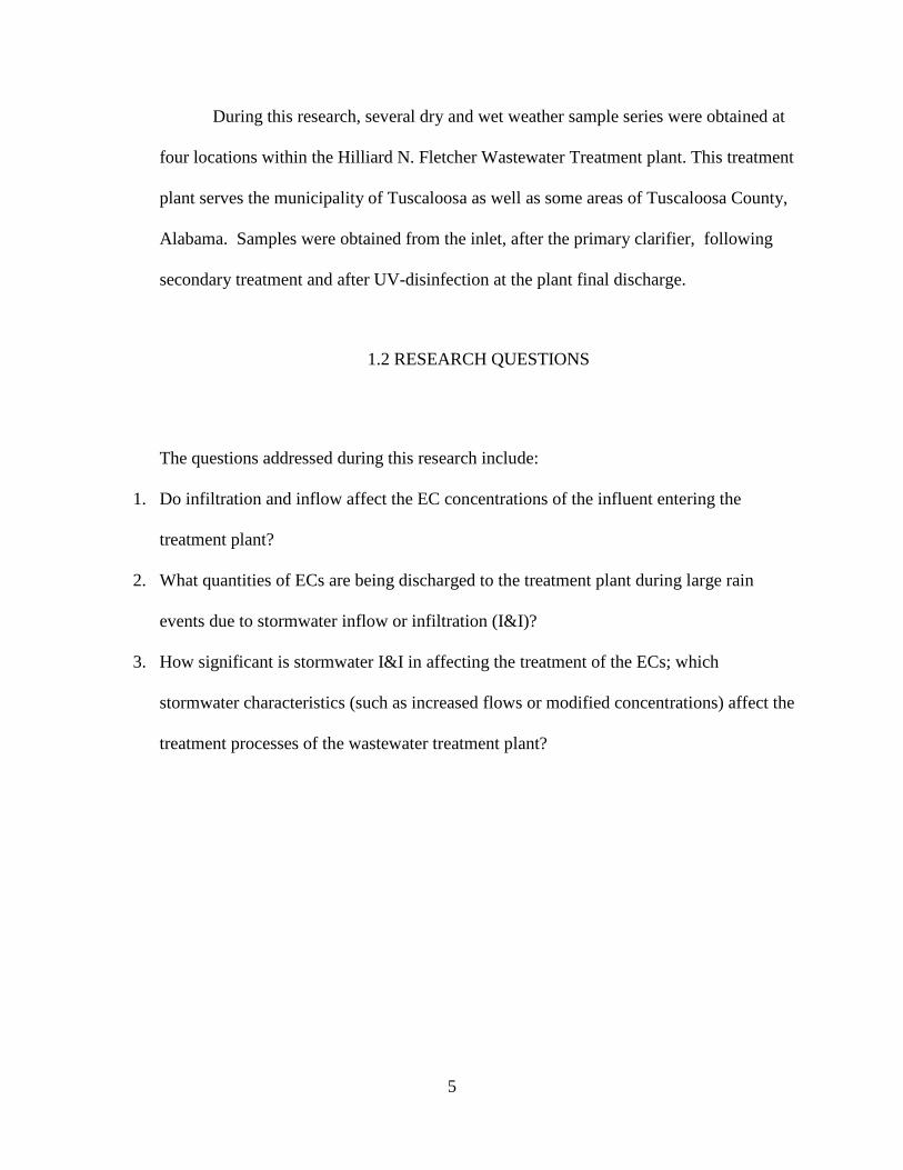
During this research, several dry and wet weather sample series were obtained at
four locations within the Hilliard N. Fletcher Wastewater Treatment plant. This treatment
plant serves the municipality of Tuscaloosa as well as some areas of Tuscaloosa County,
Alabama. Samples were obtained from the inlet, after the primary clarifier, following
secondary treatment and after UV-disinfection at the plant final discharge.
1.2 RESEARCH QUESTIONS
The questions addressed during this research include:
1. Do infiltration and inflow affect the EC concentrations of the influent entering the
treatment plant?
2. What quantities of ECs are being discharged to the treatment plant during large rain
events due to stormwater inflow or infiltration (I&I)?
3. How significant is stormwater I&I in affecting the treatment of the ECs; which
stormwater characteristics (such as increased flows or modified concentrations) affect the
treatment processes of the wastewater treatment plant?
5
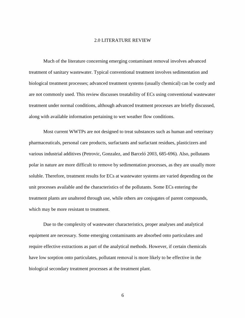
2.0 LITERATURE REVIEW
Much of the literature concerning emerging contaminant removal involves advanced
treatment of sanitary wastewater. Typical conventional treatment involves sedimentation and
biological treatment processes; advanced treatment systems (usually chemical) can be costly and
are not commonly used. This review discusses treatability of ECs using conventional wastewater
treatment under normal conditions, although advanced treatment processes are briefly discussed,
along with available information pertaining to wet weather flow conditions.
Most current WWTPs are not designed to treat substances such as human and veterinary
pharmaceuticals, personal care products, surfactants and surfactant residues, plasticizers and
various industrial additives (Petrovic, Gonzalez, and Barceló 2003, 685-696). Also, pollutants
polar in nature are more difficult to remove by sedimentation processes, as they are usually more
soluble. Therefore, treatment results for ECs at wastewater systems are varied depending on the
unit processes available and the characteristics of the pollutants. Some ECs entering the
treatment plants are unaltered through use, while others are conjugates of parent compounds,
which may be more resistant to treatment.
Due to the complexity of wastewater characteristics, proper analyses and analytical
equipment are necessary. Some emerging contaminants are absorbed onto particulates and
require effective extractions as part of the analytical methods. However, if certain chemicals
have low sorption onto particulates, pollutant removal is more likely to be effective in the
biological secondary treatment processes at the treatment plant.
6

2.1 TREATMENT AND PHYSICO-CHEMICAL PROPERTIES OF EMERGING CONTAMINANTS
Emerging contaminants include a broad range of pollutants with varying characteristics
and effects on the environment. In order to gain some understanding of how these pollutants are
removed by different unit processes, it is possible to compare them to other contaminants having
similar characteristics. Yet not all pollutants in the same category behave similarly. For
example, one may ask if all hormones are removed at the same rate during the secondary
treatment process?
There are many physicochemical properties known for emerging contaminants, but only
some are important when estimating EC behavior in treatment systems (Mauricio et al. 2006, 75-
87). The main physical and chemical properties that affect EC treatment in wastewater facilities
are the octanol/water coefficient, water solubility, pH, sorption coefficient, structure and the
molecular weight of the compound. The biological and chemical activities of pharmaceuticals
are strongly influenced by their functional groups and the pH of the solution (Nghiem, Schäfer,
and Elimelech 2005, 7698-7705). Pharmaceuticals are generally polar in nature and may have a
greater affinity to be soluble depending on the pollutant. PAHs and pesticides are more
hydrophobic than pharmaceuticals, therefore they have a higher affinity to sorb onto particulate
matter. Understanding the basic properties of contaminants in aqueous solutions gives a better
understanding of how each pollutant can be removed from water.
Analyses of organic pollutants in wastewater are complex due to the variety of
physicochemical and toxicological properties of compounds included in the same group
(Petrovic, Gros, and Barcelo 2006, 68-81). The wastewater matrix increases the complexity of
the analysis methods because of interference from other contaminants present. Each compound
7

group requires specific analysis steps (mainly extractions and sample clean-up) using different
techniques (Bolong et al. 2009, 229-246).
Research has resulted in the availability of physicochemical properties relating to
emerging contaminants, such as the octanol-water coefficient (Kow), solubility and molecular
weight. The octanol-water coefficient is a surrogate measure of how the compound may be
absorbed by organic matter.. Solubility and log Kow are inversely proportional. If pollutants have
a higher log Kow and lower solubility, they tend to sorb on organic particulate matter and can be
removed in primary treatment (sedimentation).
Although wastewater treatment plants are critical for the removal of emerging
contaminants from sanitary wastewaters, relatively little is known about the nature, variability,
transport and fate of these compounds in typical treatment facilities in the United States (Phillips
et al. 2005, 5095-5124).
2.1.1 Pharmaceuticals and personal care products (PPCPs)
Pharmaceuticals are a growing concern because there are many being introduced into
wastewater in ever-increasing amounts and variety. Many do not have discharge regulations, yet
it has been shown that trace levels of some have caused adverse effects in the environment.
Human and veterinary pharmaceuticals represent more than 4,000 commercially available
compounds; 10,000 specialty products are made to be water soluble, biodegradable and to have
short half-lives (Beausse 2004, 753-761). Pharmaceuticals have been analyzed in several studies
and detected in wastewater effluent and in the environment at trace levels. Analytical techniques
and equipment are now available that can detect pharmaceuticals at lower concentrations than
8
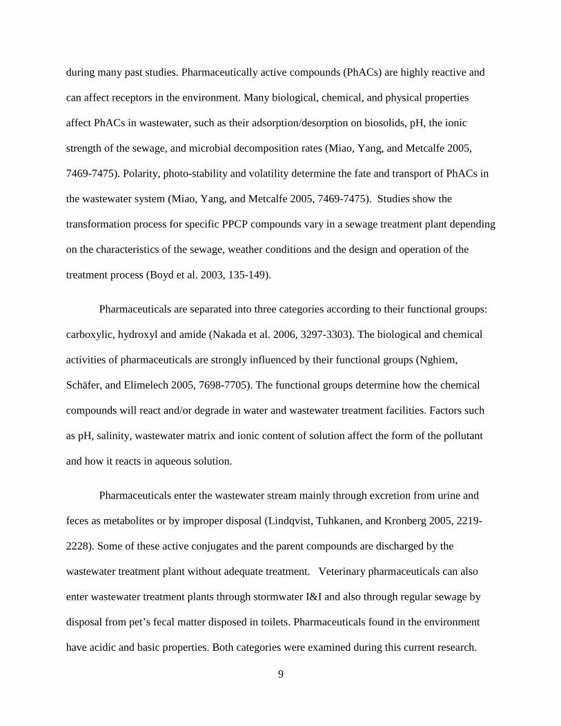
during many past studies. Pharmaceutically active compounds (PhACs) are highly reactive and
can affect receptors in the environment. Many biological, chemical, and physical properties
affect PhACs in wastewater, such as their adsorption/desorption on biosolids, pH, the ionic
strength of the sewage, and microbial decomposition rates (Miao, Yang, and Metcalfe 2005,
7469-7475). Polarity, photo-stability and volatility determine the fate and transport of PhACs in
the wastewater system (Miao, Yang, and Metcalfe 2005, 7469-7475). Studies show the
transformation process for specific PPCP compounds vary in a sewage treatment plant depending
on the characteristics of the sewage, weather conditions and the design and operation of the
treatment process (Boyd et al. 2003, 135-149).
Pharmaceuticals are separated into three categories according to their functional groups:
carboxylic, hydroxyl and amide (Nakada et al. 2006, 3297-3303). The biological and chemical
activities of pharmaceuticals are strongly influenced by their functional groups (Nghiem,
Schäfer, and Elimelech 2005, 7698-7705). The functional groups determine how the chemical
compounds will react and/or degrade in water and wastewater treatment facilities. Factors such
as pH, salinity, wastewater matrix and ionic content of solution affect the form of the pollutant
and how it reacts in aqueous solution.
Pharmaceuticals enter the wastewater stream mainly through excretion from urine and
feces as metabolites or by improper disposal (Lindqvist, Tuhkanen, and Kronberg 2005, 2219-
2228). Some of these active conjugates and the parent compounds are discharged by the
wastewater treatment plant without adequate treatment. Veterinary pharmaceuticals can also
enter wastewater treatment plants through stormwater I&I and also through regular sewage by
disposal from pet’s fecal matter disposed in toilets. Pharmaceuticals found in the environment
have acidic and basic properties. Both categories were examined during this current research.
9

The pharmaceuticals tested include sulfamethoxazole (SMX), trimethoprim (TRM), fluoxetine
(FLX), carbamazepine (CBZ), triclosan (TCL), ibuprofen (IBP) and gemfibrozil (GFB). Many of
these compounds have more than one functional group that react differently in the wastewater
treatment system. The structure, biodegradability rates, half-life, and toxicity of these
compounds all affect their treatment in the secondary biological treatment phase. Some parent
and intermediate compounds of pharmaceuticals can form hazardous byproducts during
conventional chlorination (the treatment plant studied during this research uses UV disinfection).
During this study, seven pharmaceuticals were examined at various stages at the wastewater
treatment facility. Sulfamethoxazole, fluoxetine, triclosan, ibuprofen and gemfibrozil are acidic
pharmaceuticals, while carbamazepine and trimethoprim are basic pharmaceuticals.
Table 2.1. Selected Chemical Properties of Pharmaceuticals
Pharmaceutical Log kow Solubility (mg/L)
pKa Toxicity (μg/L) Chemical Group
Carbamazepine 2.45 17.7 13.9 LC50 D. magna >100 mg/L Carboxide
Fluoxetine 4.05 38.4 9.5 P. subcapitata LC50 24 μg/L Amine
Gemfibrozil 4.78 5.0 4.7 D. Magna. EC50 23 mg/L Valeric Acid/Pentoic Acid
Ibuprofen 3.5-4.0 41.5 4.9 Daphnia. EC50 108 mg/L Propanoic acid
Sulfamethoxazole 0.9 600 1.7/5.7 P. subcapitata. IC50 1.5 mg/L Sulfonamide
Triclosan 4.8-5.4 2-4.6 7.8-8.1 P. subcapitata. IC50 1.4 μg/L Phenol
Trimethoprim 0.79 400 7.2 P. subcapitata. IC50 80- 130 mg/L
Diamine
10

Sulfamethoxazole, or 4-amino-N-(5-methylisoxazol-3-yl)-benzenesulfonamide, is an
antibiotic, generally used in conjunction with trimethoprim for bacterial infections such as
urinary tract infections. Its molecular weight is 253 g/mol and it has a solubility of 600 mg/L.
Sulfamethoxazole is a pharmaceutical of the sulfonamide group. They are also known as
sulfanilamides because of the aniline attached to it. Amides have carbonyl groups with a nitrogen
molecule. Amides are persistent and stable in nature and resist hydrolysis. They are polar
compounds so they are prone to be soluble in water. Although aniline was able to degrade
quickly, sulfanilamide degrades very slowly by aniline-acclimated activated sludge suggesting
that biodegradation in water and soil will be slow (PubMed Molecular Biology Database ).
Sulfanomides are both fairly water- soluble and polar compounds, which ionize based on the pH
of the medium (Accinelli et al. 2007, 2677-2682). Sulfamethoxazole contains two functional
moieties (-NH-S(O2) at both sides of the sulfonamide linkage (Nghiem, Schäfer, and Elimelech
2005, 7698-7705). Sulfamethoxazole is shown to dissociate twice, once with the protonation of
the primary amine group -NH2 and then with the deprotonation of the sulfanomide (-NH)
(Nghiem, Schäfer, and Elimelech 2005, 7698-7705). At pH levels above 5.7, sulfamethoxazole
remains as an anionic species, remains neutral at pH values between 1.7 and 5.7, and remains
positive at pH levels below 1.7 (Nghiem, Schäfer, and Elimelech 2005, 7698-7705). The pH of
wastewaters generally ranges between 6 and 8, which makes it neutral under normal conditions.
The log Kow is low so it is believed that sulfamethoxazole will typically remain in aqueous
solutions throughout the wastewater treatment system and will not sorb to particles. Sulfonamide
antimicrobials are not readily biodegraded (Pérez, Eichhorn, and Aga 2009, 1361-1367). In
surface waters impacted by human wastes, sulfonamides appear to resist biodegradation rather
strongly, with detection of sulfamethoxazole and trimethoprim in streams with frequencies up to
11

27% (Hazardous Substance Database 2012). In the Reconnaissance Study by the EPA and
USGS, sulfamethoxazole was categorized as a persistent antibiotic, which is possibly due to
having an aromatic structure as part of the molecule (Xu et al. 2011, 7069-7076).
Sulfamethoxazole has also been shown to be resistant to biodegradation, hydrolysis and
adsorption, but photodegradation is a possible eliminating factor (Xu 2011). The biological half-
life of sulfamethoxazole is 10 hours, but the biodegradation of sulfamethoxazole studied in
marine water ponds indicated separate water and sediment half-lives of 47.7d and 10.1 d,
respectively (DrugBank 2012);(Xu et al. 2011, 7069-7076). Toxicity of the freshwater green alga
P. subcapitata has an IC 50 of 1.5 mg/L (Yang et al. 2009, 1201-1208). Toxicities of these
compounds in wastewater were found to be in the milligrams per liter range, while the literature
indicates that wastewater concentrations range in the micrograms per liter and nanogram per liter
range.
Trimethoprim, or 5-(3,4,5- trimethoxybenzyl) pyrimidine- 2,4- diamine, is an
antimicrobial compound commonly used to treat both humans and animals (Miao et al. 2004,
3533-3541). For humans, it is generally used to treat urinary tract infections and certain types of
pneumonia. For animals, trimethoprim is mainly used in the treatment of livestock, such as pigs,
cattle and poultry and in aquaculture for bacterial infections (Mikes and Trapp 2010, 1-6). It has
a molecular weight of 290.32 g/mol. At a temperature of 25°C, it has a solubility of 400 mg/L.
Trimethoprim is classified as a diamine, with two amino groups attached to the molecule. The
molecule also has two phenol groups and three ether groups. Ethers are stable and do not react
readily unless under high temperature . Trimethoprim is a polar weak base with a pKa of 7.2, but
under acidic conditions, it is completely ionized (Mikes and Trapp 2010, 1-6). Under neutral
conditions, it has a log Kow of 0.79 but can range from -1.7 to 0.79 (acidic pH to neutral pH)
12

(Mikes and Trapp 2010, 1-6). Solubility is also contingent on the pH of the solution.
Trimethoprim in wastewater under standard temperatures and neutral pH conditions theoretically
remains in solution unless it is biodegraded in the activated sludge process. The biological half-
life in humans for trimethoprim is 10 to 11 hours, but the half-lives of trimethoprim incorporated
into sediment cores were approximately 100 and 75 days under anaerobic and aerobic conditions,
respectively, suggesting that biodegradation occurs slowly in the environment (Hazardous
Substance Database 2012; DrugBank 2012). Slow biodegradation in the environment indicates
that wastewater treatment facilities may not efficiently remove the chemical.
Fluoxetine, or N-Methyl-γ-[4-(trifluoromethyl) phenoxy]benzenepropanamine, is
classified as an amine with two benzene rings, one with the triflourine and one with an ether
connected to a chiral group. Fluoxetine is an antidepressant used in medications such as Prozac
and Sarafem. It is excreted either unchanged (20-30% unchanged) or as the metabolites
glucuromide and norfluoxetine from the human body. Some of the glucuromides are reactivate in
wastewater treatment plants by cleavage (Nentwig 2007, 163-170). Fluoxetine has a log Kow of
4.05, water solubility of 38.4 mg/L at 25˚C and vapor pressure of 8.9E-007mmHg (Nentwig
2007, 163-170). It has a high sorption rate so it should undergo some treatment in both the
primary and secondary treatment processes of the treatment facility. Fluoxetine contains
secondary aliphatic amines which are basic, indicating that they are predominatedly protonated
at neutral pH and only partially adsorb to sludge (Bedner and MacCrehan 2006, 2130-2137). The
lethal concentration at 50% (IC 50) for P. subcapitata was found to be 24 μg/L (Brooks et al.
2003, 169-183). The biological half-life is 1 to 3 days. The main metabolite from fluoxetine is
norfluoxetine.
13

Carbamazepine (CBZ), or 5H-dibenzo[b,f]azepine-5-carboxamide, is an anti-epileptic
drug with different crystalline forms, all having variable dissolutions leading to irregular and
delayed adsorption (Sethia and Squillante 2004, 1-10). Seventy-two percent of the compound is
released in urine, and various metabolites are excreted from urine into the wastewater system
(Zhang, Geißen, and Gal 2008, 1151-1161). Carbamazepine is classified as a carboxamide and is
a primary amide group. It is also known as dibenzazepine, which is a molecule with two benzene
rings fused to an azepine group (DrugBank 2012). It has a log kow value of 2.45. Carbamazepine
is a base with a pKa value of 2.3 and is uncharged at all conditions typical of natural water or
wastewater (Nghiem, Schäfer, and Elimelech 2005, 7698-7705). Carbamazepine has a low
octanol-water coefficient (Kow) and a water solubility of 17.7 mg/L (25˚C) (Nakada et al. 2006,
3297-3303; Sethia and Squillante 2004, 1-10; Zhang, Geißen, and Gal 2008, 1151-1161). Studies
on removal efficiencies of carbamazepine show that carbamazepine is difficult to remove from
sewage. Due to its persistent nature, carbamazepine has been proposed as a molecular marker for
sewage (Nakada et al. 2006, 3297-3303). At low concentrations, carbamazepine is resistant to
biodegradation (Zhang, Geißen, and Gal 2008, 1151-1161). Carbamazepine is frequently
detected in groundwater up to concentrations of 610 ng/L and in other water bodies (Zhang,
Geißen, and Gal 2008, 1151-1161). Carbamazepine has a biological half-life of 25 to 65 hours,
but was fairly persistent when tested in a field experiment using epilimnion lake water,
exhibiting a half-life of 63 days (Hazardous Substance Database 2012; DrugBank 2012).
Approximately 72% of orally administered carbamazepine is absorbed and released as
metabolites in the urine, while 28% is unchanged and subsequently discharged through the feces
(Zhang, Geißen, and Gal 2008, 1151-1161). According to the Zhang study, carbamazepine is
shown to be in many different forms in wastewater. These forms may change back into the
14

parent carbamazepine during the treatment process, which causes it to be difficult to eliminate.
The metabolites of carbamazepine may be more or less difficult to remove due to chemical
altering which may give carbamazepine different chemical properties. Research shows
carbamazepine increases in the effluent (Zhang, Geißen, and Gal 2008, 1151-1161). Metabolites
vary in their octanol water coefficient (log Kow), from 0.67 to 2.67. Most of the carbamazepine is
metabolized in the urine, with each of the metablites being as active as the parent compound.
Zhang (2008) indicated there are limited studies on the effects of the metabolites of
carbamazepine on aquatic life. The toxicity of LC 50 D. magna is >100 mg/L (Kim et al. 2007,
370-375).
Table 2.2 Log of octanol-water coefficients for carbamazepine and its metabolites
Analyte Abbreviation Formula/MW Log Kow
carbamazepine CBZ C15H12N2O/236.10 2.25 2.67 +0.38
10,11-dihydro-10,11-epoxycarbamazepine
CBZ-EP C15H12N2O2/252.09 1.26 + 0.54
10,11-dihydro-10,11-dihydroxycarbamazepine
CBZ-DiOH C15H14N2O3/270.10 0.13 + 0.41
2-hydroxycarbamazepine CBZ-2OH C15H12N2O2/252.09 2.25 + 0.65
3-hydroxycarbamazepine CBZ-3OH C15H12N2O2/252.09 2.41 + 0.73
10,11-dihydro-10-hydroxycarbamazepine
CBZ-10OH C15H14N2O2/254.10 0.93 + 0.33
Zhang 2008
Triclosan, or 5-Chloro-2-(2,4-dichlorophenoxy) phenol, is an anti-microbial compound
found in many personal care products such as soaps. The U.S. Geological Survey found triclosan
in 57% of 137 streams nationwide (Latch et al. 2005, 517-525). Triclosan is a chlorinated
phenoxyphenol with a pka of 8.1; the pH of wastewater between 7 -9 would have a significant
15

influence on its speciation (Singer et al. 2002, 4998-5004). Triclosan, a polychlorinated diphenyl
ether, has similar chemical properties to hydroxlated metabolites of ortho-substituted PCBs and
PBDEs (Cherednichenko et al. 2012, 14158-14163). PCBs are very stable in the environment
and have long half-lives. Ethers are not as soluble in water as alcohol, and are not as reactive.
Triclosan has a water solubility of about 2,000 to 4,600 µg/L at 25˚C and a high octanol/water
partition coefficient (log10 Kow) of 4.8-5.4, indicating a significant potential for sorption to
particles (Singer et al. 2002, 4998-5004; Heidler and Halden 2007, 362-369). The pKa of
triclosan indicates that this compound will exist partially in anion forms in the environment.
Anions generally do not adsorb as strongly to soils containing organic carbon and clay compared
to their neutral counterparts (Hazardous Substance Database 2012). Even though its dissociated
form tends to degrade in sunlight, triclosan is quite resistant to hydrolysis (Singer et al. 2002,
4998-5004). It is converted, either by UV radiation or photohydrolysis, into 2, 8-
dichlorodibenzo-p-dioxin (2, 8-DCDD, a dioxin) (Latch et al. 2005, 517-525). Methyl triclosan,
a potential biotransformation product following wastewater treatment of triclosan, is more
persistent, lipophilic, bio-accumulative and less sensitive towards photo-degradation in the
environment than its parent compound (Chen et al. 2011, 452-456). Also, exposure of triclosan
to freshwater green alga P. subcapitata yielded an IC 50 of 1.4 μg/L (Yang et al. 2009, 1201-
1208). In aerobic water-sediment systems maintained in darkness at 20 ± 2°C, triclosan degraded
with calculated nonlinear half-lives of 1.3 to 1.4 days in water, 54 to 60 days in sediment, and 40
to 56 days in the total system (U.S. Environmental Protection Agency 2008).
Ibuprofen, or α-Methyl-4-(2-methylpropyl) benzene-acetic acid, is a non-steroidal anti-
inflammatory drug (NSAIDS). The classification of this compound is a propanoic acid.
Propanoic acids are soluble in water and can react with many other compounds. Ibuprofen can
16
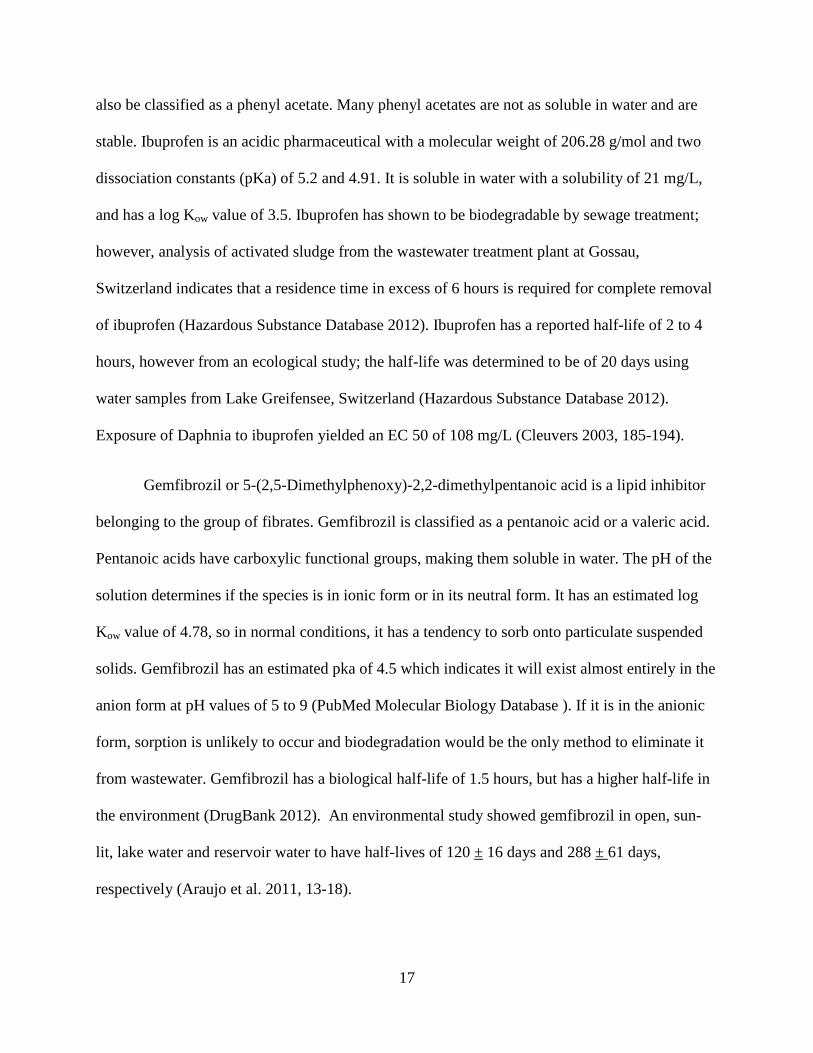
also be classified as a phenyl acetate. Many phenyl acetates are not as soluble in water and are
stable. Ibuprofen is an acidic pharmaceutical with a molecular weight of 206.28 g/mol and two
dissociation constants (pKa) of 5.2 and 4.91. It is soluble in water with a solubility of 21 mg/L,
and has a log Kow value of 3.5. Ibuprofen has shown to be biodegradable by sewage treatment;
however, analysis of activated sludge from the wastewater treatment plant at Gossau,
Switzerland indicates that a residence time in excess of 6 hours is required for complete removal
of ibuprofen (Hazardous Substance Database 2012). Ibuprofen has a reported half-life of 2 to 4
hours, however from an ecological study; the half-life was determined to be of 20 days using
water samples from Lake Greifensee, Switzerland (Hazardous Substance Database 2012).
Exposure of Daphnia to ibuprofen yielded an EC 50 of 108 mg/L (Cleuvers 2003, 185-194).
Gemfibrozil or 5-(2,5-Dimethylphenoxy)-2,2-dimethylpentanoic acid is a lipid inhibitor
belonging to the group of fibrates. Gemfibrozil is classified as a pentanoic acid or a valeric acid.
Pentanoic acids have carboxylic functional groups, making them soluble in water. The pH of the
solution determines if the species is in ionic form or in its neutral form. It has an estimated log
Kow value of 4.78, so in normal conditions, it has a tendency to sorb onto particulate suspended
solids. Gemfibrozil has an estimated pka of 4.5 which indicates it will exist almost entirely in the
anion form at pH values of 5 to 9 (PubMed Molecular Biology Database ). If it is in the anionic
form, sorption is unlikely to occur and biodegradation would be the only method to eliminate it
from wastewater. Gemfibrozil has a biological half-life of 1.5 hours, but has a higher half-life in
the environment (DrugBank 2012). An environmental study showed gemfibrozil in open, sun-
lit, lake water and reservoir water to have half-lives of 120 ± 16 days and 288 ± 61 days,
respectively (Araujo et al. 2011, 13-18).
17

The physical and chemical characteristics are varied for all pharmaceuticals, including
the analytes under study. The solubilities of some of the pharmaceuticals in wastewater make
them more difficult to treat. Depending on the pH of the wastewater, many micropollutants can
exist in ionized or unionized aqueous forms (Myers 2009). Dissociation constants or pKa values
help predict the behavior of pharmaceuticals in the environment. For acidic pharmaceuticals,
pKa values lower than the pH of the wastewater will yield an ionized compound that can easily
be absorbed. For basic pharmaceuticals, pKa values higher than pH of wastewater will yield an
ionized compound. If ionization of a pollutant is not significant, sorption would be a likely
means of treatment. If a species is not ionized, the solubility is decreased, and sorption,
biodegradation and/or oxidation could be the method of removal. If the log Kow values are high
(>3), sorption is a viable mechanism. The stability of the compounds is determined by their
chemical structure and composition and affects their treatment in wastewater. In an activated
sludge treatment system, toxicity of certain chemical compounds can inhibit the microbes that
biodegrade the pollutants in wastewater.
2.1.2 Polycyclic Aromatic Hydrocarbons
Polycyclic aromatic hydrocarbons are compounds derived from petroleum products such
as tar, oil and coal and are byproducts of burning these materials. They are comprised of several
benzene rings. As petroleum products are combusted, many PAHs are emitted in the atmosphere.
PAHs are ubiquitous environmental pollutants with carcinogenic and mutagenic properties that
can have adverse effects if exposed to humans (Busetti et al. 2006, 104-115). Stormwater
transports PAHs from sources such as asphalt, oil and gas usage, and from wet and dry
18

atmospheric deposition. PAHs can enter sanitary wastewater through I&I. In this study, the
monitoring of typical stormwater PAHs at the wastewater treatment facility will help determine
their treatability under both dry and wet weather conditions. PAHs are differentiated by the
number of rings and the placement of hydrocarbons connected to the rings reveal physical and
chemical properties. At wastewater treatment facilities, PAHs can undergo changes in physical
and chemical compositions. PAHs are typically insoluble in water and are very lipophilic. Due
to their strong hydrophobic characteristics, PAHs are mostly removed from wastewaters during
the activated sludge treatment process through sorption onto particulates that are then removed
from the wastewater by sedimentation (Busetti et al. 2006, 104-115).
PAHs are divided into two groups: those with low molecular weights and those with high
molecular weights. PAHs containing four or fewer rings are easier to biodegrade than PAHs with
five rings or greater (Hazardous Substance Database 2012). PAHs such as naphthalene and
acenaphthene both have low molecular weights. Acenaphthene is also a non-carcinogenic EPA
priority pollutant with a two-ring chemical structure. Acenaphthene and naphthalene are easily
biodegradable because they are lower in molecular weight and have smaller ring structures. With
solubility in water of 31.7 mg/L and a Henry's law constant of 4.6x10⁻⁴; it is likely that
volatilization will be an important route of naphthalene loss from water (ATSDR 2011 2011).
PAH compounds such as benzo(a)pyrene and chrysene have more cyclic rings and have higher
molecular weights. There is a correlation between increasing molecular weight of these
compounds and decreasing solubility. Anthracene and pyrene have three to four cyclic carbon
rings, causing an increase in sorption capacity and reduction in aqueous solubility. Fluoranthene
has a slightly higher molecular weight and is highly lipophilic, with a log Kow of 5.14 and
solubility of 0.20 to 0.26 mg/L (Crunkilton and DeVita 1997, 1447-1463). Chrysene has a high
19

molecular weight of 228.3 g mol-1, log Kow of 5.16, and solubility of 2.8µg/L (ATSDR 2011
2011). PAHs such as benzo[b]fluoranthene (log Kow=6.04) and benzo[a]pyrene (log Kow=6.06)
all have very high log octanol-water coefficients and correspondingly very low solubilities. The
toxicities of PAHs have a wide range. Many are above the concentration ranges found at
wastewater treatment plants as indicated in the literature and from the experimental data during
this research.
Table 2.3. Characteristics of PAHs
Compound Molecular
weight
(g/mol)
Solubility
(water)(mg/L)
Log kow Volativity
atm-3/mol
Toxicity **
naphthalene 128.2 31.7* 3.37*
4.6x10-4 *
LC50
Pimephales
promelas
7.76 mg/L
acenaphthylene 152.2 3.93* 3.89** 1.45 x 10⁻³ *
acenaphthene 154.2 1.93* 4.02** 7.91 x 10⁻⁵ * LC50 Salmo
gairdneri
1570 μg/L
fluorene 166.2 1.68-1.98 * 4.12** 1.0 x 10⁻⁴ * EC 50 V.
fischeri 4.10
μg/mL
anthracene 178.2 0.076 * 4.53** 1.77 x 10⁻⁵ * D.magna EC
50=211 μg/L
phenanthrene 178.2 1.20 * 4.48** 2.56 x 10⁻⁵ * EC50; Daphnia magna 678.41 µg/L
pyrene 202.2 0.077 * 5.12** 1.14 x 10⁻⁵ * D.magna EC
50=67000
μg/L
20
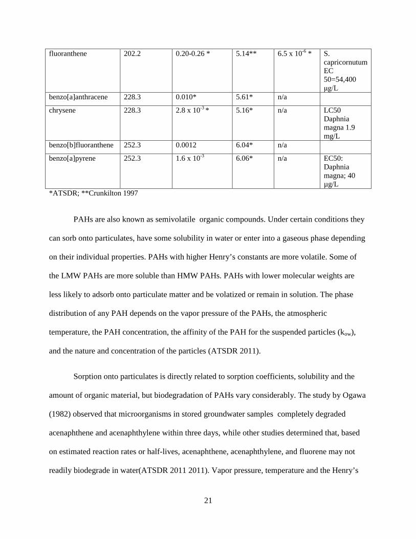
fluoranthene 202.2 0.20-0.26 * 5.14** 6.5 x 10⁻⁶ * S. capricornutum EC 50=54,400 μg/L
benzo[a]anthracene 228.3 0.010* 5.61* n/a
chrysene 228.3 2.8 x 10-3 * 5.16* n/a LC50 Daphnia magna 1.9 mg/L
benzo[b]fluoranthene 252.3 0.0012 6.04* n/a
benzo[a]pyrene 252.3 1.6 x 10⁻³ 6.06* n/a EC50: Daphnia magna; 40 µg/L
*ATSDR; **Crunkilton 1997
PAHs are also known as semivolatile organic compounds. Under certain conditions they
can sorb onto particulates, have some solubility in water or enter into a gaseous phase depending
on their individual properties. PAHs with higher Henry’s constants are more volatile. Some of
the LMW PAHs are more soluble than HMW PAHs. PAHs with lower molecular weights are
less likely to adsorb onto particulate matter and be volatized or remain in solution. The phase
distribution of any PAH depends on the vapor pressure of the PAHs, the atmospheric
temperature, the PAH concentration, the affinity of the PAH for the suspended particles (kow),
and the nature and concentration of the particles (ATSDR 2011).
Sorption onto particulates is directly related to sorption coefficients, solubility and the
amount of organic material, but biodegradation of PAHs vary considerably. The study by Ogawa
(1982) observed that microorganisms in stored groundwater samples completely degraded
acenaphthene and acenaphthylene within three days, while other studies determined that, based
on estimated reaction rates or half-lives, acenaphthene, acenaphthylene, and fluorene may not
readily biodegrade in water(ATSDR 2011 2011). Vapor pressure, temperature and the Henry’s
21

constant are other properties that may affect how PAHs are treated throughout the unit processes
of the treatment plant, but log kow is most likely to be the most important parameter indicating
their treatability.
2.1.3 Pesticides and Herbicides
Pesticides and herbicides are used to reduce damaging or nuisance insects, weeds or other
pests that have a negative impact on agriculture or public health. Chemical pesticides contributed
to increased yields of agriculture by controlling pests and diseases (AHMAD et al. 2010, 231-
271); however, excessive amounts of pesticides can have detrimental effects on wildlife and
human populations. Highly chlorinated pesticides are known as persistent organic pollutants
(POPs). POPs tend to have low water and high fat solubility, stability during degradation
processes, low vapor pressure and are persistent in the environment (Katsoyiannis and Samara
2004, 2685-2698). Pesticide contaminants enter wastewater treatment plants by surface runoff
from treated sites, in contaminated rinses from cleaning of pesticide applicators and containers,
and/or from disposal of unused pesticides (Monteith et al. 1995, pp. 964-970).
The major types of pesticides are organochlorine pesticides and organophosphorus
pesticides. Of these categories, they are divided into four types: insecticides, fungicides,
herbicides and bactericides (Badawy, Ghaly, and Gad-Allah 2006, 166-175). Chlorinated
phenoxy acid herbicides, which account for the majority of pesticides worldwide, are
characterized by high polarity and thermal lability (Petrovic, Gonzalez, and Barceló 2003, 685-
696).
22

Organochlorine pesticides are known for their persistence in the environment and their
bioaccumulation in the food chain (Jiries, Al-Nasir, and Beese 2002, 97-107) .
Organophosphorus pesticides degrade faster in the environment than organochlorine pesticides
(Jiries, Al-Nasir, and Beese 2002, 97-107). Researchers in Switzerland analyzed the fate and
transport of azole fungicides and found the fungicides were unaffected by wastewater treatment.
Azole fungicides in wastewater are moderately lipophilic and fairly persistent with half-lives of
weeks to months (Kahle et al. 2008, 7193-7200). Chlorinated hydrocarbon pesticides and
chlorophenoxy herbicides are used worldwide and have been detected in the nanogram per liter
and microgram per liter levels in almost every major U.S. river and lake (Saleh, Lee, and Wolf
1980, 19-28). In the Selah study, total 2,4D was found in the Dallas wastewater treatment plant
study. 2, 4-D, butoxyethyl ester and 2, 4-D, isooctyl ester have a water solubility of 10-12 mg/L.
2, 4-D, isopropyl ester has a higher solubility at 46 mg/L and also may not be effectively
removed at wastewater treatment plants, depending on biodegradation. The pesticides
prochloraz, flusilazole and epoxiconazole have relatively high log Kow values of 4.38, 3.7 and 3.4
respectively. Although these values generally indicate these compounds are highly lipophilic and
less soluble, studies at several wastewater treatment plants show they were not significantly
removed.
Most likely, pesticide sources entering the wastewater treatment plant are from
stormwater I&I entering the wastewater treatment plant. A number of pesticides are implicated
as endocrine disruptors in aquatic and wildlife species (U.S. EPA 2001 ).
23
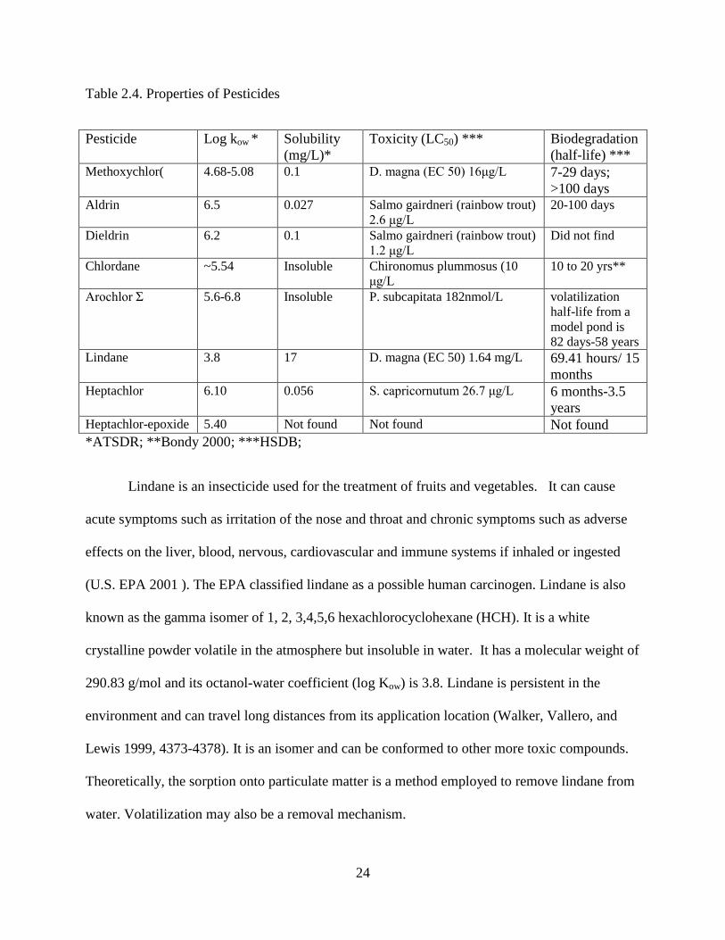
Table 2.4. Properties of Pesticides
Pesticide Log kow * Solubility (mg/L)*
Toxicity (LC50) *** Biodegradation (half-life) ***
Methoxychlor( 4.68-5.08 0.1 D. magna (EC 50) 16μg/L 7-29 days; >100 days
Aldrin 6.5 0.027 Salmo gairdneri (rainbow trout) 2.6 μg/L
20-100 days
Dieldrin 6.2 0.1 Salmo gairdneri (rainbow trout) 1.2 μg/L
Did not find
Chlordane ~5.54 Insoluble Chironomus plummosus (10 μg/L
10 to 20 yrs**
Arochlor Σ 5.6-6.8 Insoluble P. subcapitata 182nmol/L volatilization half-life from a model pond is 82 days-58 years
Lindane 3.8 17 D. magna (EC 50) 1.64 mg/L 69.41 hours/ 15 months
Heptachlor 6.10 0.056 S. capricornutum 26.7 μg/L 6 months-3.5 years
Heptachlor-epoxide 5.40 Not found Not found Not found *ATSDR; **Bondy 2000; ***HSDB;
Lindane is an insecticide used for the treatment of fruits and vegetables. It can cause
acute symptoms such as irritation of the nose and throat and chronic symptoms such as adverse
effects on the liver, blood, nervous, cardiovascular and immune systems if inhaled or ingested
(U.S. EPA 2001 ). The EPA classified lindane as a possible human carcinogen. Lindane is also
known as the gamma isomer of 1, 2, 3,4,5,6 hexachlorocyclohexane (HCH). It is a white
crystalline powder volatile in the atmosphere but insoluble in water. It has a molecular weight of
290.83 g/mol and its octanol-water coefficient (log Kow) is 3.8. Lindane is persistent in the
environment and can travel long distances from its application location (Walker, Vallero, and
Lewis 1999, 4373-4378). It is an isomer and can be conformed to other more toxic compounds.
Theoretically, the sorption onto particulate matter is a method employed to remove lindane from
water. Volatilization may also be a removal mechanism.
24

Chlordane is an organochlorine insecticide that contains a complex mixture of more than
forty-five individual isomers and congeners (Kawano et al. 1988, 792-797). Chlordane was first
produced in 1947 and used as an insecticide. The EPA banned chlordane in 1988 because it was
found to be a carcinogen, causing ecological damage (U.S. Environmental Protection Agency ).
Chlordane has an environmental half-life of ten to twenty years (Bondy et al. 2000, 386-398).
Because it is fat soluble, it can enter animal tissue and accumulate, causing harmful effects in
humans. Chlordane acts as an endocrine disrupting compound, having estrogenic effects on
human breast cells. Thus, chlordane mimics biological activities of hormones, such as the
hormone 17β-estradiol (Bonefeld-Jørgensen et al. 2001, 141-153). The hormone 17β-estradiol is
important for stimulating breast cell proliferation in mature breast tissue (Bonefeld-Jørgensen et
al. 2001, 141-153). Pure chlordane has a molecular weight of 409.76 g/mol. It has a low water
solubility and high log Kow value (~5.54). At wastewater treatment facilities, it is expected that
most of the chlordane would be removed because it tends to sorb to particulates.
Methoxychlor is an insecticide that replaced the carcinogen DDT. It is a pale yellow solid
with a light odor. When created commercially, between 88-90% of the pesticide is pure
methoxychlor (ATSDR 2011 ). It is virtually insoluble in water and it binds to soil when applied
to plants (ATSDR 2011 ). The log Kow of methoxychlor is approximately 4.68 to 5.08, which is
relatively high. EPA does not classify methoxychlor as a carcinogen, but it does simulate
estrogens in the body which affects the reproduction of certain species. Methoxychlor causes a
negative impact to the nervous system if it is exposed directly.
Heptachlor is an insecticide used extensively in the past for killing insects in homes,
buildings and on food crops (ATSDR 2011). Application of the insecticide ceased in 1988 and is
now permitted only for fire ant control in underground power transformers (ATSDR 2011).
25

Heptachlor epoxide is formed from the breakdown of heptachlor by bacteria and animals
(ATSDR 2011). It is more soluble in water than heptachlor and it very persistent in the
environment. EPA classified both heptachlor and heptachlor epoxide as possible human
carcinogens. Both chemicals are a white solid with camphor like odor. The molecular weights
are 373.32 g/mol for heptachlor and 389.40 g/mol for heptachlor epoxide. The log Kow for
heptachlor is 6.10 and the log Kow for heptachlor epoxide is 5.40. It binds to soil and is expected
to be treated by wastewater treatment facilities primarily by sedimentation.
Aldrin and dieldrin are organochlorine pesticides commercially manufactured since 1950.
They were used throughout the world until the early 1970s (International Labour Organisation,
United Nations Environment Programme, and World Health Organization 1988). Aldrin breaks
down into dieldrin which kills disease carrying insects, such as the tsetse fly. Since the early
1970s, the two compounds are severely restricted or banned in several countries, especially in
agriculture (International Labour Organisation, United Nations Environment Programme, and
World Health Organization 1988). Nevertheless, they are still used in some other countries for
termite control (International Labour Organisation, United Nations Environment Programme,
and World Health Organization 1988). Both aldrin and dieldrin are insoluble in water (although
dieldrin has higher solubility) having a relatively high molecular weight being 364.91 g/mol and
380.91 g/mol respectively. Both compounds have high log Kow values, 6.5 and 6.2 respectively.
Both aldrin and dieldrin often bind to particulates and are expected to be removed through
sedimentation processes.
Arochlor is a mixture of several polychlorinated biphenyl (PCB) congeners sold in the
U.S. from 1930 to 1977 (ATSDR 2011 ). The Aroclors are identified by a four-digit numbering
code in which the first two digits indicate the type of mixture and the last two digits signify the
26

approximate chlorine content by weight percent (ATSDR 2011 ). Thus, Aroclor 1242 is a
chlorinated biphenyl mixture of varying amounts of mono- through heptachlorinated homologs
with an average chlorine content of forty-two percent (ATSDR 2011 ). The exception to this
code is Aroclor 1016, which contains mono- through hexachlorinated homologs with an average
chlorine content of forty-one percent (ATSDR 2011 ).
Table 2.5. Physical and Chemical Properties of Aroclors (ATSDR 2011 )
Arochlor congener Molecular weight (g/mol)
Solubility (water) (mg/L) at 25°C
Vapor pressure (mm Hg) at 25°C
Henry’s Constant (atm-m3/mol) at 25°C
Log Kow
1016 257.9 0.42 4 x 10⁻⁴ 2.9 x 10⁻⁴ 5.6
1221 200.7 0.59 (24°C) 6.7 x 10⁻³ 3.5 x 10⁻³ 4.7
1232 232.2 0.45 4.06 x 10⁻³ No data 5.1
1242 266.5 0.34 4.06 x 10⁻³ 5.2 x 10⁻⁴ 5.6
1248 No data No data No data No data No data
1254 328 0.012 7.71 x 10⁻⁵ 2.0 x 10⁻³ 6.5
1260 357.7 0.0027 4.06 x 10⁻⁵ 4.6 x 10⁻³ 6.8
1262 389 0.052 (24°C) No data No data No data
1268 453 0.300 (24°C) No data No data No data
All of the Arochlor congeners are insoluble in water and have a high affinity for oil and fat.
They have very high molecular weights and the octanol-water coefficients are high for all of
them. PCBs tend to sorb on to particulate matter rather than dissolve in aqueous solutions and are
therefore likely to be removed at wastewater treatment plants by sedimentation.
2.1.4 Endocrine disruptors
27

As noted above, some personal care products (PPCPs), pharmaceuticals, synthetic
estrogens, and pesticides imitate natural estrogens that affect the endocrine system. These
chemicals are called endocrine disruptor chemicals (EDCs). The United States’ EPA defines an
EDC as “an exogenous agent that interferes with the synthesis, secretion, transport, binding,
action, or elimination of natural hormones of natural hormones in the body that are responsible
for the maintenance of homeostatis, reproduction, development, and/or behavior” (Campbell et
al. 2006, 1265-1280).
Hormones are classified as endocrine disrupting compounds because they cause
hormonal abnormalities in aquatic wildlife such as fish. Many EDCs have moderate to high log
Koc values, so they tend to sorb to sediments or suspended solids (Campbell et al. 2006, 1265-
1280). In their sediment associations, there is the potential for biological uptake, degradation and
transformations to less or more mobile forms (Campbell et al. 2006, 1265-1280). The solubility
values suggest they would not stay in solution; however, most EDCs are identified in water
samples (Campbell et al. 2006, 1265-1280). Campbell (2006) also found a poor correlation
between colloidal partitioning coefficient and the water octanol partitioning coefficients (log
Kow), indicating the dominant mechanism for the binding of EDCs to colloidal particles may not
be controlled by its log Kow.
Estrogens are one of the main endocrine disruptors present in influent and effluent at
wastewater treatment facilities. The most common synthetic hormone used for contraceptives is
17 α-ethynylestradiol, with concentrations being 30 to 50 µg per pill (Beausse 2004, 753-761).
Synthetic compounds with estrogenic activity include 17α-ethinylestradiol (EE2), and
alkylphenol polyethoxylates (NPnEO) (Teske and Arnold 2008, 107-124). In the Teske literature
review, chemical and biological characteristics such as chemical structure, molecular weight,
28

water solubility at 20C and the log Kow are listed. Estrogens have low solubility and high log Kow
values that suggest sorption is a key component in the removal of estrogen during wastewater
treatment.
Table 2.6. Properties of Endocrine Disruption Chemicals
EDC Molecular weight (g/mol)
Water solubility at 20C (mg/L)
Log Kow
Estrone (E1) 270.4 13 3.43
17β-Estradiol (E2) 272.4 13 3.94
Estriol (E3) 288.4 13 2.81
Ethinyl Estradiol (EE2)
296.4 4.8 4.15
Bisphenol A 228.0 300 3.40
Octylphenol (OP) 206.3 12.6 4.12
Nonylphenol (NP) 220.0 5.43 4.48
Nonylphenol polyethoxylates (n>3-5)
352.0-440.0 5.88-9.48 4.2-4.3
Nonylphenoxy ethoxy acetic acid
322 soluble 1.34
(Teske and Arnold 2008, 107-124)
Campbell’s (2006) review showed estradiol exhibits log Koc of 2.55-4.01 L/kg; water solubility
of 13.0-32 mg/L and pKa of 10.5-10.71. The same literature shows 17β-Estradiol (E2) has
similar properties of log Koc 3.10-4.01 and water solubility of 13.0 mg/L. The estrogens have low
solubility and moderately high octanol-water partitioning coefficient. The log kow that are
generally above 3 suggest they would not remain in solution. Some studies show estrogens
29
present in the effluent and not sorbed to particulates. Campbell (2006) argue: (1) there are more
soluble precursors of metabolites being transport (i.e. nonylphenol carboxylics); (2) there is more
colloid facilitated transport; (3) there is an enhanced solubility through elevated pH (many e-
EDCS have a pka around 10); and (4) there is the formation of micelles which can greatly
enhance the stability of the compound.
In some of the literature, commonly measured physicochemical properties are not always
the best predictors affecting the treatment behavior of EDCs. Literature records other factors that
could be pivotal in predicting EDC removal in wastewater treatment facilities. Researchers found
certain EDCs were reduced in wastewater systems due to the increase of sludge retention time.
Some compounds are transformed throughout the treatment process. Seasonal conditions could
affect the treatability of wastewater systems.
2.2 WASTEWATER TREATABILITY IN CONVENTIONAL WWTP
2.2.1 Description of wastewater unit processes
Wastewater in a conventional treatment system goes through five different unit treatment
processes that incorporate sedimentation, sorption, biodegradation (or degradation), and
disinfection. Depending on the chemical properties of the constituent, one or more of these
processes will reduce the compound’s concentration. . The five steps of the treatment systems are
(1) pre-treatment; (2) grit-removal; (3) primary treatment; (4) secondary treatment; and (5)
disinfection.
30

Pre-treatment is the removal of large particles that could potentially clog a system and
cause significant damage. In toilets, large objects are flushed in the sewer lines. In sewers, items
as large as animals can pass through. Sanitary sewers are not designed to treat plastic items, cans,
bottles, large paper items or large organic matter. The pre-treatment screen removes coarse solids
to ensure debris does not enter the treatment plant and interfere with plant operations. For
emerging contaminants that cause adverse effects at low concentrations, pre-treatment provides
little benefit for the direct removal of these contaminants.
Pre-treatment may include a sand or grit channel or chamber where the velocity of the
incoming wastewater is adjusted to allow the settlement of sand, grit, stones, and broken glass.
These particles are removed because they may damage pumps and other equipment. For
emerging contaminants, grit removal may remove a small portion of the ECs that are sorbed onto
the larger particles. PAHs are known to sorb onto particulate matter (especially organics). For
emerging contaminants in aqueous forms, there is no treatment during the grit removal process.
The sorption of these chemicals is mostly to organic solids having low specific gravities, while
the grit removal units are designed more for mineral based particulates that have very rapid
settling characteristics.
Primary treatment, particularly in a biological treatment facility, involves the settling of
particles and suspended solids from the aqueous solution. There likely is some treatment of
certain emerging contaminants in this process. PAHs tend to sorb to particles and organic
material due to their hydrophobic nature. The higher the molecular weight, the more likely it will
sorb on to particle material. PAHs with lower molecular weights may remain in solution.
Pollutants with a log Kow of 3 or more theoretically sorb to solid or organic materials. Synthetic
and natural hormones and surfactants found in wastewaters tend to have high log Kow values and
31

will therefore tend to sorb to particulates. However, if these pollutants are in an oxidized or
metabolic form, characteristics of the parent compound may not be applicable. If
pharmaceuticals and personal care products are in acidic or basic forms, depending on the pH,
they will remain in aqueous solution.
Secondary Treatment
During this dissertation research, treatability was examined at a conventional activated
sludge wastewater treatment facility. Secondary treatment uses microbial organisms for the
consumption (stabilization) of organic pollutants entering the treatment facility. Organic
pollutants are therefore removed primarily by biodegradation. Some PPCPs, pesticides and
EDCs are only partially removed using microbial action. Removal efficiency is dependent on
several factors, such as physicochemical properties, the operation and design of the treatment
facility (hydraulic and sludge retention time) and weather conditions and other seasonal
variations (seasonal flow patterns and temperature).
Disinfection
Disinfection is the last phase in the treatment process of wastewaters before the final
discharge of the effluent from a treatment facility. Disinfection is used to reduce the amounts of
pathogenic microorganisms in the effluent. There are different methods of disinfection used at
wastewater treatment facilities. Chlorination is one of the most common methods used, although
chlorine can react with organic matter to form harmful compounds. Ultraviolet light and ozone
are other means of disinfection for wastewater treatment. UV treatment damages the genetic
structure of bacteria, viruses and pathogens, making them unable to reproduce. Ozone
disinfection oxidizes the organics in the wastewater, destroying microorganisms that are present,
32
but does not have a residual effect as does chlorine. The disinfection treatment used at the
Tuscaloosa wastewater treatment system is UV light. Typically, the oxidation occurring in the
disinfection process can further reduce organic pollutants (such as ECs).
2.2.2 Wastewater treatment of emerging contaminants as reported in the literature
The first section of this literature review focuses on the characteristics of each category of
emerging contaminants. Retention time affects the treatability of the emerging contaminants and
can offer an explanation to the treatability and fate of compounds under normal conditions. In
this section, studies are reviewed for conventional municipal treatment systems, a membrane
bioreactor (MBR) treatment system and combined sewer systems. There is very little information
on treatability of ECs from stormwater entering wastewater treatment facilities, which this
research is addressing.
During this dissertation research, the treatability of each compound examined for normal
climatic conditions is analyzed to gain an understanding of how rain events generally affect
certain chemicals through both literature reviews and monitoring activities.
2.2.2.1 Pharmaceuticals
During the Gobel (2007) study, samples were taken from two wastewater treatment
systems, Kloten-Opfikon (WWTP-K) and Altenrhein (WWTP-A), near Zurich, Switzerland. The
Kloten-Opfikon plant treats wastewater from about 55,000 population equivalents (PE): the
combined sewage of 25,900 residents, and of an unknown number of air traffic passengers in the
catchment area (Göbel et al. 2007, 361-371). The average inflow (dry weather) is 16,500 m3/d.
33

The primary treatment consists of pre-treatment and a primary clarifier. Sixty-percent of the
primary effluent is further treated by an activated sludge treatment system that operates at a
sludge age of three days and a hydraulic retention time of 5 hours (V=2,500 m3). The main
conventional activated sludge treatment (CAS-K) includes denitrification (V=1,900 m3) and
nitrification (V=3,700 m3) with a solid retention time of 10–12 d. The hydraulic retention time
(HRT), including the secondary clarifier, is about 15 h. A membrane bioreactor pilot plant is
operated in parallel to the CAS-K facility, using primary effluent at a flow rate proportional to
raw water influent (HRT about 13 h). The bioreactor consists of a stirred anaerobic compartment
(V=6 or 8 m3) and a denitrification (V=4 m3) and nitrification (V=6 m3) cascade. The solid
retention time was increased between the sampling campaigns from 16±2 to over 33±3 d (steady
state operation for two to three sludge ages prior to sampling).
The Altenrhein wastewater treatment plant treats the wastewater from 80,000 population
equivalents, including 52,000 inhabitants. Primary treatment consists of pretreatment and a
primary clarifier. Secondary treatment is performed in two parallel operated treatment units: a
conventional activated sludge (CAS-A) and a fixed-bed reactor (FBR), receiving approximately
fifty percent of the primary effluent each (Göbel et al. 2007, 361-371). Both systems are
designed for nitrification and denitrification. Conventional activated sludge treatment includes a
denitrifying volume (anoxic, mixed) of 2,300 m3 and nitrifying (aerobic) volume of 6,800 m3.
The solid retention time in the CAS-A system ranged between 21 d to 25 d, while no value was
available for the FBR. The hydraulic retention time was approximately 31 h for the CAS-A
including the secondary clarifier, whereas it ranged below 1 h for the FBR.
34

Gobel et al 2007 investigated the treatment of sulfanomides, macrolides and trimethoprim
in conventional activated sludge systems and in fixed bed reactor systems. Table 5 gives a list of
the reduction rates for the primary treatment process.
Table 2.7. Reduction rates of ECs by primary sedimentation treatment
Compound Acronym CASRN Percentage removal (%) n=9
Sulfapyridine SPY 144-83-2 -29 to 20
Sulfamethoxazole SMX 723-46-6 -21 to -5
N4-acetylsulfamethoxazole
N4AcSMX
SMX + N4AcSMX
21312-10-7 9 to 21
0 to 9
Trimethoprim TRI 738-70-5 -13 to 31
Azithromycin AZI 83905-01-5 10 to 33
Erythromycin ERY-H2O 114-07-8 -8 to 4
Roxithromycin ROX 80214-83-1 3 to 9
(Göbel et al. 2007, 361-371)
The Gobel study showed a high degree of variability in the removal of each of the ECs
during primary treatment. Sulfamethoxazole concentrations are shown to increase in all samples
during primary treatment. This is perhaps caused by the simultaneous presence of compounds
that have been deconjugated, substances such as human metabolites of these compounds in the
influent (Göbel et al. 2007, 361-371). N4-acetylsulfamethoxazole had reductions ranging from
9% to 21% during primary treatment.
During secondary treatment, the variability increased even more compared to primary
treatment. The March 2002 data demonstrates an increase in sulfapyridine and sulfamethoxazole
during the secondary treatment. The metabolite of sulfamethoxazole, N4-
acetylsulfamethoxazole, showed a very high removal percentage. In each of the conventional
35

treatment sludge systems investigated, the metabolite N4-acetylsulfamethoxazole had the highest
reductions. The low removal rates for this study are likely a result of conjugation and
deconjugation of the targeted compounds.
Table 2.8. EC reduction rates during secondary treatment (%)
Percentage reduction
WWTP-K WWTP-K WWTP-K WWTP-A WWTP-A
N = 3 for each period
March 2002 February 2003
November 2003
September 2002 March 2003
SPY -74 + 66 -16 + 45 -107 + 8 49 + 5 72 + 5
SMX -107 + 8 9 + 3 -79 + 7 -138 + 15 60 + 3
N4AcSMX
SMX + N4AcSMX
94 + 2
50 + 3
87 + 1
53 + 1
90 + 1
-1 + 3
96 + 2
61 + 3
85 + 1
76 + 1
TRI 3 + 5 -1 + 6 14 + 5 20 + 11 -40 + 20
AZI No results -26 + 8 -18 + 7 55 + 4 22 + 11
ERY-H2O 6 + 4 -14 + 4 -22 + 4 -6 + 8 -9 + 8
CLA 9 + 4 -45 + 7 -7 + 5 4 + 7 20 + 6
ROX 18 + 4 38 + 3 -18 + 6 38 + 5 5 + 8
(Göbel et al. 2007, 361-371)
In the Castiglioni (2006) study, six different wastewater treatment plants were observed
with varying flow rates and population. Table 8 is a summary of the influent and effluent loads
of all six treatment facilities. All six of the wastewater facilities were conventional activated
sludge treatment plants with standard pre-treatment and primary treatment.
Table 2.9. Characteristics of wastewater treatment plants studied by Castiglioni et al (2006)
36

STP Population Flow rate MGD Type of waste treated
Cagliari 270,000 22.9 domestic
Naples 840,000 47.8 domestic
Latina 45,000 5.0 domestic
Cuneo 140,000 8.2 domestic
Varese Olona 120,000 6.1 domestic
Varese Lago 110,000 10.5 domestic and industrial
(Castiglioni et al. 2006, 357-363)
The Castiglioni research found that ibuprofen, sulfamethoxazole and carbamazepine all
had relatively low to moderate removal rates. Ibuprofen and sulfamethoxazole were not
associated with particulates, and showed moderate removal rates of 55 percent and 24 percent
respectively. Although carbamazepine was associated with the particulate matter, it had zero
percent removals. The apparent effluent loads for carbamazepine increased compared to the
influent loads which possibly indicates some chemical activity occurred through the unit
processes, such as potentially liberating the compound from particulate matter, or changes in the
presence of interfering compounds through the treatment processes.
Table 2.10. Summary of EC Loads and Removal Rates at Wastewater Treatment Facilities
Pharmaceuticals Load in influent (mg/d/1000 inh)
Removal rate in STP (%)
Residual load in effluent(mg/d/1000 inh)
Occurrence in particulate (+/-) *
atenolol 494 21 281 +
ofloxacin 360 57 233 +
Ibuprofen 122 55 28 -
Sulfamethoxazole 65 24 10 -
37

Carbamazepine 12 0 28 +
(Castiglioni et al. 2006, 357-363) *presence or absence of pharmaceutical (qualitative)
The wastewater treatment plant in the Rosal (2010) study is located in Alcala de Henares
in Madrid, Spain. This plant treats a mixture of domestic and industrial wastewater with a
capacity of 3,000 m3/h (33,020 gpd) (Rosal et al. 2010, 578-588).The facility serves a population
of more than 10,000 inhabitants. It uses secondary biological treatment, although they do not
specify which biological treatment process was used. The treatment plant had an influent pH of
7.54 (0.24) and effluent pH of 7.63 (0.17) (Rosal et al. 2010, 578-588). Treatment takes place in
anaerobic, anoxic and oxic zones. This study showed that gemfibrozil and triclosan possessed
the highest removal rates, at 76 percent and 75 percent, respectively. Trimethoprim and
carbamazepine showed the lowest removal rates at 5.1% and 9.5%, respectively. For most
compounds, the removal rates during biological treatment increased with higher hydrophobicity
with many non-polar substances being sorbed to the sludge.
Table 2.11. Dissociation Constants, Influent and Effluent Concentrations of ECs
Compound Caffeine Carbamazepine Gemfibrozil Naproxen Sulfamethoxazole Triclosan Trimethoprim
pKa 10.4 13.9 4.7 4.2 5.7 7.8 6.8
Influent (ng/L) Max Min Avg
65 x 103 173 17 x 103 5228 530 2417 197
5 x 10³ 106 415 1196 162 <LOQ 78
23 x 103 129 3.5 x 10³ 2363 279 860 104
Effluent (ng/L) Max Min Avg
1589 173 5233 2208 370 512 148
<LOQ 69 3 359 104 <LOQ <LOQ
1176 117 845 923 231 219 99
Removal Efficiency (%)
94.5 9.5 76.0 60.9 17.3 74.5 5.1
38

(Rosal et al. 2010, 578-588)
Lishman (2006) studied twelve wastewater treatment facilities. Treatment processes used
included lagoons, activated sludge, and activated sludge with filtration. The treatment facilities
treated residential and industrial wastewaters. Average daily flow rates ranged from 1,984 m3/d
to 105,300 m3/d. All activated sludge systems studied used primary clarification. Table 11 is a
compilation of the plant systems’ influent and effluent concentrations. Table 12 shows the
percent reductions of activated sludge treatment systems for this study.
Table 2.12. Influent and Effluent Concentrations, Detection Limits and Percent Reductions
Analyte MDL (µg/L)
Point source
Median (µg/L)
Mean (µg/L)
Maximum (µg/L)
Percent reductions (%)
Ibuprofen 0.061 Influent 8.84 8.45 16.5 Effluent 0.353 0.384 0.773 95.4% Gemfibrozil 0.077 Influent 0.418 0.453 0.965 Effluent 0.255 0.246 0.436 45.7% Naproxen 0.074 Influent 5.22 5.58 17.1 Effluent 0.351 0.452 1.189 91.9% Triclosan 0.031 Influent 1.86 1.93 4.01 Effluent 0.106 0.108 0.324 94.4% Diclofenac 0.062 Influent 0.140 0.204 1.01 Effluent 0.140 0.194 0.748 4.9% (Lishman et al. 2006, 544-558)
The Lishman study reported ibuprofen and triclosan removal rates of more than 90
percent, while gemfibrozil and diclofenac had very low removals. Gemfibrozil and diclofenac
both have been shown in the literature to have moderate removals: 46 percent (Lishman et al.
2006, 544-558) and 69 percent (Ternes 1998, 3245-3260)(Lishman et al. 2006, 544-558). Clara
et al (2003) showed moderate removals for diclofenac and gemfibrozil of between 53 percent
and 74r percent (Lishman et al. 2006, 544-558). Eight of the twelve WWTP under investigation
39

were conventional wastewater treatment systems. The others were lagoon wastewater treatment
systems.
Ibuprofen and triclosan all had higher removals at conventional wastewater treatment
facilities. Ibuprofen has the highest removals with low variability. Naproxen and triclosan both
had relatively high removal percentages, but triclosan has a slightly higher variability between
the conventional treatment systems. Gemfibrozil varied in concentration removal but overall, it
was lower than seventy percent. Some of the removal rates were as low as 38 percent.
Table 2.13. Percent reductions of ECs at conventional activated sludge wastewater treatment facilities CAS plant IBP NPX GMF DCF TCL
4 95 79 43 -88 74
5 98 96 ### **# 98
6 ### 95 69 22 97
7 94 86 38 -103 93
8a 98 98 ### ### 93
8b 94 81 66 28 85
9 91 90 71 -143 89
10 ### 98(#) ### 77 98
(Lishman et al. 2006, 544-558); *--number of times there was non-quantifiable values; #--measurable in the influent and non-quantifiable in the effluent
Miege (2009) prepared a comprehensive literature review, compiling wastewater
treatment removal data for ECs from 117 publications. Table 12 is a summary of the treatment
plant data for conventional activated sludge facilities. This review examined the targeted
emerging contaminants and also the metabolites of carbamazepine. For this set of data,
ibuprofen and naproxen had high removals ranging from 87 percent to 94 percent. Trimethoprim
had a medium removal rate of 74 percent. Triclosan, gemfibrozil and sulfamethoxazole all had
40

lower removal rates of less than 70 percent. Carbamazepine had a 30 percent removal rate and
their metabolites ranged from negative 80 percent to 51 percent, consistent with other literature
values. Ibuprofen shows relatively high removal rates in the literature. There is significant
variability of each analyte, possibly a result of each contaminant’s physical and chemical
properties.
Table 2.14. Comparison of Influent and Effluent and Percentage Reductions for ECs Analyte Sample
location Median (µg/L)
Mean (µg/L)
Min (µg/L)
Maximum (µg/L)
n Frequency of quantification (%)
Percent reduction (%)
Ibuprofen Influent 3.20 14.6 0.170 83.5 3 100 Effluent 0.800 1.96 0.0020 24.6 109 93 86.5 Gemfibrozil Influent 1.49 1.63 0.700 3.00 4 25 Effluent 0.600 0.564 0.0600 1.34 21 70 65.4 Naproxen Influent 6.00 26.4 1.79 611 45 96 Effluent 0.880 1.89 0.170 33.9 53 87 92.8 Triclosan Influent ***** 0.380 ***** ***** 1 100 Effluent 0.130 0.150 0.0700 0.430 19 100 60.5 Diclofenac Influent 0.997 1.34 0.105 4.11 91 81 Effluent 0.420 0.680 0.0350 1.95 101 85 49.2 CBZ-10OH Influent ***** 0.0222 ***** ***** 3 100 Effluent ***** 0.0325 ***** ***** 3 100 -46.3
CBZ-2OH Influent ***** 0.0390 ***** ***** 3 100 Effluent 0.0704 3 100 -80.5 CBZ-3OH Influent ***** 0.0554 ***** ***** 3 100 Effluent ***** 0.0692 ***** ***** 3 100 -24.9 CBZ-DiOH Influent ***** 1.001 ***** ***** 3 100 Effluent ***** 1.08 ***** ***** 3 100 -7.9 CBZ-EP Influent ***** 0.0392 ***** ***** 3 100 Effluent ***** 0.0191 ***** ***** 3 100 51.3 Carbamazepine Influent 0.732 0.968 0.100 1.90 64 100 Effluent 0.520 0.674 0.150 2.30 63 100 30.4 Sulfamethoxazole Influent 0.157 0.342 0.0200 1.25 10 71 Effluent 0.0700 0.115 0.0180 0.320 11 73 66.4 Trimethoprim Influent 0.281 0.449 0.0800 1.30 10 100 Effluent 0.0600 0.118 0.0200 0.550 27 93 73.7 (Miege et al. 2009, 1721-1726); *****no value reported
Radjenovic (2007) did a comparison of the treatability between a membrane bioreactor
system (MBR) wastewater system and a conventional activated sludge (CAS) treatment system.
The MBR is a suspended growth activated sludge system that uses microporous membranes for
41

solid/ liquid separations instead of secondary clarifiers (Stephen Chapman and Law ). A MBR of
approximately 21 L active volume equipped with two flat sheet membranes was installed in a
municipal WWTP. Although the nominal porosity of the membrane was 0.4μm, a fouling layer
of proteins and microorganisms formed on the surface, reduced the effective porosity to 0.01μm
(Radjenovic, Petrovic, and Barceló 2007, 1365-1377). The MBR was operated in parallel with
the aeration tank and secondary settling tank. The Rubi CAS wastewater treatment plant was
designed for a population of 125,550. The WWTP was operating with an average daily flow rate
of 22,000 m3/d. The treatment plant was designed to treat municipal, hospital and industrial
wastewater. Treatment was a biological activated sludge system with standard pretreatment and
primary treatment. The hydraulic retention time was approximately 12 hours and the sludge
retention time was approximately three days.
There is a greater variability in removal for all of the compounds for CAS facilities.
Gemfibrozil had the largest differences in treatability with the MBR removal at 90 percent and
the CAS removal at 39 percent. Diclofenac showed an 80 percent t removal for MBR facilities,
while removal at the CAS facilities was only 50 percent. Carbamazepine showed no removal for
either treatment system. Ibuprofen, naproxen and sulfamethoxazole displayed small differences
in removals between the treatment plant types.
Table 2.15. Comparison of Membrane Bio Reactor and Conventional Activated Sludge**
Compound Elimination percentage
MBR CAS
Analgesic/Anti-inflammatory drugs
Naproxen 99.3(1.52) 85.1(11.4)
Ibuprofen 99.8(0.386) 82.5(15.8) Diclofenac 87.4(14.1) 50.1(20.1) Anti-epileptic drugs Carbamazepine No elimination No elimination Antibiotic
42

Sulfamethoxazole 60.5(33.9) 55.6(35.4) Lipid Regulator/Cholesterol lowering statin drug
Gemfibrozil 89.6(23.3) 38.8(16.9) **(Radjenovic, Petrovic, and Barceló 2007, 1365-1377)
This dissertation research did not investigate hormones, but their reported treatability
offers some insight on the treatment potential of other ECs. Some personal care products act as
EDCs, thus understanding their behavior in wastewater treatment systems is important.
Hormones have a range of log Kow values but tend to range above three. . Andersen et al (2003)
observed removals of estrogen at one conventional activated sludge facility. The project
examined the municipal wastewater treatment plant in Wiesbaden, Germany. The primary
effluent is directed to an activated sludge system for biological and chemical treatment, including
phosphate removal, denitrification, and nitrification (Anderson et al. 2003, 4021-4026).
Fe(II)Cl2 is added in the first denitrification tank for efficient mixing in the water before
oxidation to Fe(III) and subsequent precipitation with phosphate in the aerated nitrification tanks.
After settling in the secondary clarifier, the activated sludge is returned to the inlet of the first
denitrification tank. The secondary effluent is discharged into the river Rhine. The activated
sludge system is operated with a solids retention time of 11-13 d, which is typical for a nitrifying
plant with predenitrification. The range of concentrations for E1, E2, and EE2 were in the
nanograms per liter range throughout the treatment system. When being treated in the primary
clarifier, there was an increase in E1 concentrations and in the combination of E1 and E21. This
is possibly due to the hormones reacting with each other and metabolites in the primary clarifier.
All hormones showed almost total removal after nitrification and denitrification. Hormones were
significantly reduced only after biological treatment.
43
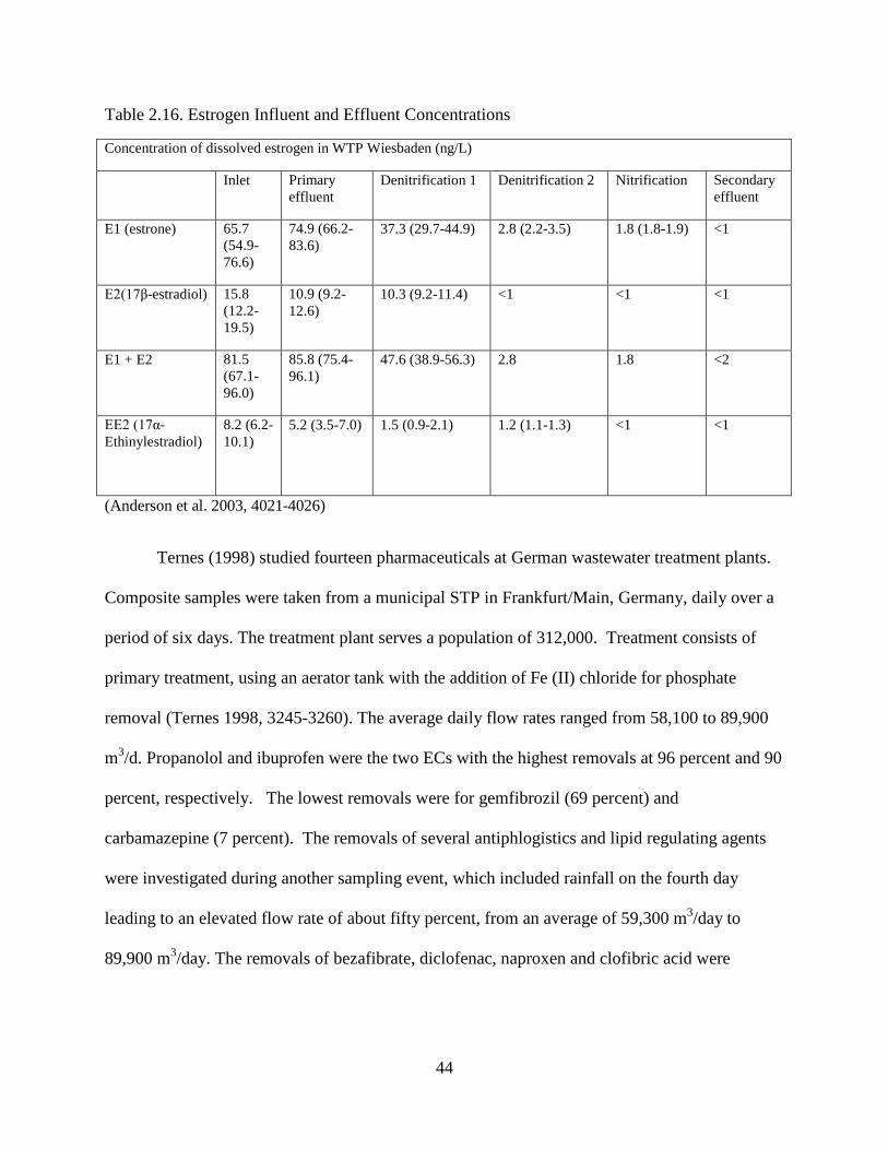
Table 2.16. Estrogen Influent and Effluent Concentrations
Concentration of dissolved estrogen in WTP Wiesbaden (ng/L)
Inlet Primary effluent
Denitrification 1 Denitrification 2 Nitrification Secondary effluent
E1 (estrone) 65.7 (54.9-76.6)
74.9 (66.2-83.6)
37.3 (29.7-44.9) 2.8 (2.2-3.5) 1.8 (1.8-1.9) <1
E2(17β-estradiol) 15.8 (12.2-19.5)
10.9 (9.2-12.6)
10.3 (9.2-11.4) <1 <1 <1
E1 + E2 81.5 (67.1-96.0)
85.8 (75.4-96.1)
47.6 (38.9-56.3) 2.8 1.8 <2
EE2 (17α-Ethinylestradiol)
8.2 (6.2-10.1)
5.2 (3.5-7.0) 1.5 (0.9-2.1) 1.2 (1.1-1.3) <1 <1
(Anderson et al. 2003, 4021-4026)
Ternes (1998) studied fourteen pharmaceuticals at German wastewater treatment plants.
Composite samples were taken from a municipal STP in Frankfurt/Main, Germany, daily over a
period of six days. The treatment plant serves a population of 312,000. Treatment consists of
primary treatment, using an aerator tank with the addition of Fe (II) chloride for phosphate
removal (Ternes 1998, 3245-3260). The average daily flow rates ranged from 58,100 to 89,900
m3/d. Propanolol and ibuprofen were the two ECs with the highest removals at 96 percent and 90
percent, respectively. The lowest removals were for gemfibrozil (69 percent) and
carbamazepine (7 percent). The removals of several antiphlogistics and lipid regulating agents
were investigated during another sampling event, which included rainfall on the fourth day
leading to an elevated flow rate of about fifty percent, from an average of 59,300 m3/day to
89,900 m3/day. The removals of bezafibrate, diclofenac, naproxen and clofibric acid were
44
significantly reduced on the rainfall day and only bezafibric (<5% reduction) recovered by the
sixth day.
These results indicate that rainfall affected the treatment, possibly by reduced residence
times in the unit processes, reduced microbial activity, or altered sorption and/or flocculation
conditions in this rainfall period (Ternes 1998, 3245-3260). Joss (2005) noted that biological
removal varied strongly from compound to compound, with no evident correlation to the
compound structure. Ibuprofen was removed to below the quantification limit at the outfall
(>90% removal). There was no removal for carbamazepine or sulfamethoxazole (although there
was significant removal of the metabolite N4-acetyl- sulfamethoxazole). The data did not show
whether biological transformations occurred because the estimated elimination is significantly
smaller than the data accuracy (95 percent confidence interval) (Joss et al. 2005, 3139-3152).
Removal rates for each compound observed for pharmaceuticals had high variabilities for
the different compounds. Ibuprofen consistently had high removals for each study, while
sulfamethoxazole and triclosan showed varying removals (triclosan ranged from 61 to 94%,
while sulfamethoxazole ranged from -140 to 66 percent removals. Sulfamethoxazole has more
than one form and possibly undergoes chemical alteration in the treatment process. Gemfibrozil
and carbamazepine has lower variability removals, but at consistently lower values. Estrogen
activity in wastewater has been examined during some studies ((Teske and Arnold 2008, 107-
124; Anderson et al. 2003, 4021-4026). Estrogen was included in this literature review because
they are identified as endocrine disruptor chemicals. They are also biological active showing
similarity to pharmaceuticals and personal care products. Their removals in wastewater treatment
facilities, based on their physical and chemical characteristics, are similar to pharmaceutical
removals.
45
2.3 COMBINED SEWER SYSTEMS
In order to better understand how wet weather flows affect municipal wastewater
treatment facilities, one should examine performance at treatment facilities for combined sewers.
Wastewater that enters combined sewers consists of both raw sewage and stormwater.
Stormwater increased inflow is similar to municipal sewers during wet weather from I&I.
Combined sewers are single drainage systems than simultaneously collect stormwater and
wastewater in the same collection system. During dry weather, the sanitary wastewater is drained
to the treatment plant, but during wet weather, the combined flows commonly exceed the
treatment plant’s capacity, and the excess overflow is discharged mostly untreated to the
receiving water.
In combined sewers, the stormwater affects the concentrations of the pollutants in the
influent to the treatment plant (likely decreasing the concentrations of most PPCPs, while
increasing concentrations of PAHs and pesticides), and increase the flows being treated, with
associated decreased residence times in the treatment unit processes. In addition, combined
sewer overflows (CSOs) occur with the discharge of untreated influent when the flows exceed
the capacity of the treatment plant. (Weyrauch et al. 2010, 4451-4462) reported CSOs occurring
when rain events exceeded 4.7 mm (0.19 in). Numerous studies emphasize the importance of
pollutant loads conveyed by combined wet weather discharges and their adverse impacts on
receiving waters (Kafi et al. 2008, 539-549). Also, in Kafi’s study, there was an increase in
suspended solids, organic matter and hydrocarbon concentrations. A decrease was found in
heavy metal concentrations at the outfall during wet weather periods.
46

Boyd et al (2004) found concentrations of ibuprofen and triclosan in urban receiving
water canals in New Orleans after 7 cm or more rainfalls (Phillips and Chalmers 2009, 45-57).
Phillips et al (2009) reported that the concentrations and numbers of organic wastewater
compounds were higher in storm flow samples collected than in baseflow samples: 1.5 to 9.4
µg/L in stormwater and 0.05 to 0.17 µg/L in baseflow samples.
PAHs in Combined Sewer Overflows (CSOs)
One objective of this project is to determine if PAHs are entering the treatment plant at
different concentrations during wet and dry weather and how each unit treatment process
provides treatment. PAHs are divided into two categories: low molecular weight (LMW) PAHs
and high molecular weight (HMW) PAHs. There does appear to be a correlation between the
reductions of PAHs and their molecular weights (Manoli and Samara 1999, 176-186).
Table 2.17. PAH Categories
Low Molecular Weight PAHs High Molecular Weight PAHs
Naphthalene Benzo(a)anthracene Acenaphthene Pyrene Acenaphthylene Benzo(a)pyrene Fluorene Chrysene Phenanthrene Benzo(b)flouranthene Anthracene Fluoranthene
Blanchard (2001) tested samples from five combined sewer wastewater treatment plants
near Paris, France. The effluents were collected from the five sewers entering the Ache`res. The
average flow rates were: (1) 220,000 m3/d (58.1 MGD) for the Se`vres 1-Ache`res Rueil;(2)
360,000 m3/d (95.1 MGD) for the Saint Denis-Ache`res (3); 900,000 m3/d (237 MGD) for the
47

Clichy-Ache`res junction of Argenteuil; (4) 600,000 m3/d (159 MGD) for the Clichy-Ache`res
junction of Bezons and (5) 600,000 m3/d (159 MGD) for the Se`vres 2-Ache`res junction of
Saint-Cloud Nanterre (Blanchard et al. 2001, 3679-3687). Samples from the Ache’res were taken
during both dry weather and for wet weather. Atmospheric fallout was also monitored for this
study.
Figure 2.1. Comparison of dry and wet weather concentrations for total PAHs
(Blanchard et al. 2001, 3679-3687)
Blanchard (2001) observed a relationship between influent PAH concentrations during
two dry weather events and during two wet weather events at four wastewater treatment plants in
the same area. They found PAHs increase in the influent to the treatment plant during large rains
due to stormwater influences.
Pham (1997) collected samples from the Montreal, Canada Urban Community (MUC)
wastewater treatment system. The MUC wastewater treatment plant receives combined domestic,
industrial and stormwater wastewaters since its opening in 1988 (Pham and Proulx 1997, 1887-
48

1896). The MUC wastewater treatment plant serves approximately 1.4 million people (out of a
total population of 1.8 million), and approximately 15 percent of its total flow is contributed by
industry (Pham and Proulx 1997, 1887-1896). There are two intercepting areas connected to the
plant: (1) the north and southwest sector of Montreal Island and the (2) southeast sector. The
MUC treatment plant treats 1.3 million m3/day, (343 MGD), however the southeast sector was
only partially collected. Under heavy rainfall conditions, this flow rate can triple. The capacity
for this facility, including the southeast sector is 2.8 million m3/d (740 MGD).
Pham (1997) investigated several PAHs and their removals. Each PAH showed a variety
of reductions. Naphthalene had the lowest reductions which indicate minimal sorption to
particulate matter and also low biodegradation. Naphthalene has a low molecular weight and is
one of the more soluble PAHs, so there may be aqueous forms of it throughout the treatment
plant. Many of the low molecular weight compounds, such as fluorene, anthracene and
phenanthrene, had moderate removals, ranging from 57 to 65 percent. Acenaphthylene is a LMW
PAH, but during these observations, it had high removals. Chrysene had the highest removals, at
93 percent. It is a high molecular weight PAH so it was consistent with the theory that most of
HMW PAHs are removed in the primary sedimentation stage.
Table 2.18. Mean, Standard Deviations and Removal Percentages of Influent and Effluent
N=10 N=6 Avg Influent
µg/L std Influent µg/L
Avg Effluent µg/L
std Effluent µg/L
Average Removal rates %
Naphthalene 0.147 0.084 0.088 0.049 40 Acenaphthylene 0.021 0.051 0.002 0.005 90 Acenaphthene 0.016 0.011 0.005 0.003 67 Fluorene 0.037 0.025 0.015 0.008 59 Phenanthrene 0.333 0.228 0.109 0.055 67 Anthracene 0.028 0.034 0.012 0.007 58
49

Fluoranthene 0.150 0.193 0.020 0.007 86 Pyrene 0.138 0.157 0.023 0.007 83 Chrysene 0.080 0.122 0.005 0.002 93 (Pham and Proulx 1997, 1887-1896)
Manoli (1999) collected samples from the Thessaloniki, Greece combined sewage
wastewater treatment plant. It is a conventional activated sludge treatment facility which
includes the addition of a flocculant and chlorine dioxide for disinfection. The plant receives a
dry weather flow of approximately 40,000 m3/d, consisting mainly of the residential discharges
from the city of Thessaloniki (Manoli and Samara 1999, 176-186). The treatment unit processes
include: (1) pre-treatment with aerated sands and grease removal units; (2) a primary
sedimentation tank with a detention time of three hours, (3) an aeration tank with surface aerators
with a detention time of three hours, and a secondary sedimentation tank with a detention time of
6 hours.
Table 2.19. PAH Concentrations through each unit process (µg/L)
Pollutant Influent Primary effluent
Secondary effluent
Final effluent
Percent reduction
naphthalene 7.3 7.6 5.7 5.0 32 acenaphthene 0.7 0.3 0.17 0.11 84
fluorene 0.7 0.5 0.5 0.23 67 phenanthrene 1.7 0.57 0.18 0.2 88 pyrene 0.47 0.12 0.07 0.06 87 benzo(a)anthracene 0.05 0.015 0.0052 0.0047 91 chrysene 0.16 0.033 0.014 0.015 91 (Manoli and Samara 1999, 176-186)
Each of the PAHs varied in removal. In Table 17, naphthalene showed the lowest
removal rate. Naphthalene also showed an increase in the primary effluent, before its reduction
in the secondary and final treatment process. Benzo(a)anthracene and chrysene had the highest
50

reduction rates. Most of the two compounds were removed during primary treatment. These
compounds were higher in molecular weight, which imply sorption was likely the primary
removal mechanism for those compounds. The lower molecular weight PAHs are more likely to
be removed in the secondary treatment part of the facility.
Pesticides in CSOs
Pesticides have a high affinity for particulate matter, degrade at a slow rate and are
insoluble in water. The combined sewage wastewater treatment plant of the city of Thessaloniki,
Greece, serves about 1 million residents by treating 120.000–150.000 tons/d of wastewater
(Katsoyiannis and Samara 2004, 2685-2698). About five to ten percent of the total flow comes
from industrial dischargers. The treatment process includes screening, grid removal, primary
sedimentation without use of chemical coagulants, conventional activated sludge treatment and
effluent disinfection using Cl2. During the Katsoyiannis (2004) study, much of the pesticide
concentrations were reduced during both the primary and secondary treatment processes. This is
consistent with their physicochemical properties, albeit other factors affect treatment, such as
retention time. Although there were significant removals for all pesticides observed, most of the
concentrations in the secondary effluent ranged from 10-25 ng/L.
51

Figure 2.2 Concentrations of pesticides;
(Katsoyiannis and Samara 2004, 2685-2698)
Polychlorobiphenyls (PCBs) are discharged by various industries as congener mixtures.
Blanchard (2004) conducted a study of PAH and PCB concentrations from five combined sewers
near Paris entering the Ache`res region: (1) the Se`vres 1-Ache`res Rueil (220,000 m3/d or 58.1
MGD), (2) the Saint Denis-Ache`res (360,000 m3/d or 95.1 MGD); (3) the Clichy-Ache`res
junction of Argenteuil (900,000 m3/d or 237 MGD), for the Clichy-Ache`res junction of Bezons
(600,000 m3/d or 158 MGD), and the Se`vres 2-Ache`res junction of Saint-Cloud Nanterre
(600,000 m3/d or 158 MGD). Arochlor, which is a polychlorinated biphenyl, were observed by
Blanchard (2004) to be significantly reduced during the primary treatment process.
52

Figure 2.3. Concentration of ƩPCBs
(Blanchard et al. 2004, 184-197)
2.4 FINDINGS FROM THE LITERATURE AND NEED FOR RESEARCH
The literature show that combined sewers during wet weather conditions have increased
influent pollutant concentrations for many ECs and increased concentrations in the treated
effluent. Municipal wastewater treatment systems, affected by large amounts of stormwater I&I,
could have a similar effect. An important part of this dissertation research is therefore to directly
monitor changes in treatment plant conditions and performance during wet weather.
Emerging contaminants are a growing concern and understanding their behavior at
wastewater treatment facilities during both wet and dry weather is important. Almost all
available literature pertains to dry weather performance. To better understand treatability of the
ECs, chemical behavior needs to be known and treatability needs to be related to their physical
and chemical properties if modeling of removal is to be improved. Solubility and log Kow values
53

are important when studying these compounds in aqueous solutions. However, literature reports
indicate a high level of variability in treatment performance even for compounds with similar
solubilities and log Kow values. Although there is significant variability, each study presents an
illustration of how effective treatment plants are in eliminating these compounds. Gemfibrozil
and fluoxetine have high log Kow values, hence are predicted to have a large portion sorbed onto
particles (and therefore likely removed by sedimentation processes). Carbamazepine and
sulfamethoxazole have low log Kow values so they are expected to remain in aqueous solutions
under neutral conditions. Reported carbamazepine removals range from zero to 45 percent,
indicating resistance to biodegradation in conventional activated sludge systems. Triclosan and
ibuprofen showed removals between 60 and 90 percent, coinciding with the chemical
characteristics of these compounds. Gemfibrozil has a high octanol-water coefficient, and data
indicate removal rates ranging between 35 percent and 76 percent.
Phillip (2009) and Benotti (2007) reported that during heavy rainfalls, reductions
occurred in the concentrations of the examined pharmaceuticals compared to the concentrations
under dry weather conditions. For Benotti (2007), seven ECs exhibited lower concentrations
under wet conditions than during dry conditions: caffeine, carbamazepine, codeine, cotinine,
paxanthine, sulfamethoxazole, and trimethoprim. Blanchard (2001) conducted a study that
showed an increase in concentrations of PAHs and PCBs entering the treatment plant during
large rain events. The concentration ranges for each of the studied compounds were large;
however the data indicated which compounds typically were not effectively treated in standard
conventional wastewater treatment systems.
During a rain event with a large volume of stormwater infiltrating the wastewater system,
changes could affect how each unit process affects the pollutants. From the studies reported, it is
54
apparent that stormwater infiltration itself can be a major contributor of some of the ECs, even
pharmaceuticals and personal care products. Dilution can occur and reduce the concentrations of
other pollutants, resulting inadequately treated conditions due to reductions in residence times in
the unit processes.
2.5 SUMMARY OF LITERATURE REVIEW
Table 19 summarizes the chemical characteristics and their treatability as reported in the
preceding literature review for constituents being examined. This table shows the most likely
means of removal, the ranges of influent and effluent concentrations and the ranges of the
percentage removals for each constituent.
The pharmaceuticals gemfibrozil, ibuprofen, triclosan and fluoxetine were reduced by
biodegradation. The overall range of influent concentrations ranged from 0.3 to 14.6 μg/L. The
removals for these compounds varied. Ibuprofen showed the highest level of treatability ranging
from 82 to 95 percent. Triclosan had reduction rates of 75 percent and gemfibrozil had a
reduction range from 38 to 76 percent.
Carbamazepine had the lowest reported reduction rates of zero to 30 percent. .
Carbamazepine is difficult to treat, as it is resistant to biodegradation. Because carbamazepine is
soluble in water, it is also not treatable by sedimentation in the primary unit processes.
Carbamazepine concentration increases in the effluent compared to the influent were observed.
Possible treatment mechanisms of carbamazepine are not clearly understood.
Sulfamethoxazole is highly soluble in water and therefore difficult to remove.
Photodegradation removes sulfamethoxazole at some treatment facilities. The reported influent
55

concentrations ranged from 0.25 to 0.35 μg/L, and the effluent concentrations ranged from 0.11
to 0.23 μg/L. The reduction rates of sulfamethoxazole ranged from 17 to 66 percent.
Low molecular weight (LMW) PAHs (naphthalene, acenaphthene, acenaphthylene,
fluorene, phenanthrene, and anthracene) had reported reduction rates between 31 and 91 percent.
Naphathlene had the lowest reduction rates ranging from 31 to 40 percent. Naphthalene has a
Henry’s Law constant of 0.019 atm-m3/mol, making it more volatile than the other PAHs and
more likely to volatize during wastewater treatment. Acenaphthene, acenaphthylene, fluorene,
phenanthrene and anthracene have Henry’s Law constants of about 10-3, and their solubilities
range from 0.045 to 16.1 mg/L. Volatization and oxidation were the primary means of reported
treatment for PAHs having lower molecular weights. High molecular weight (HMW) PAH
compounds (such as pyrene, fluoranthene, chrysene, and benzo(a)pyrene) had higher reduction
percentages ranging from 83 to 91 percent. Adsorption is a primary removal factor for the
HMW compounds. Influent concentrations for LMW PAHs ranged from 0.016 to 7.3 μg/L.
Effluent concentrations for LMW PAHs had a range from 0.002 to 0.7 μg/L. Influent
concentrations for the HMW PAHs ranged from 0.044 to 0.47 μg/L. Effluent concentrations for
HMW PAHs ranged from 0.013 to 0.06 μg/L.
56

Table 2.20a. Summary of Characteristics and Treatability of Targeted Pollutants
Constituent Log Kow
Solubility (mg/L)
pka Biodegradation half-life * **rate
Toxicity
Pharmaceuticals Gemfibrozil 4.78 5.0 4.7 1.5 hours EC 50 D.
Magna 22.85 mg/L
Ibuprofen 3.5-4.0
41.5 4.9 2 hours EC 50 Daphnia. 108 mg/L
Triclosan 4.8-5.4
2-4.6 7.8 125 hours IC 50 P. subcapitata. 1.4 μg/L
Carbamazepine 2.25 17.7 13.9 10-20 hours LC 50 D. magna >100 mg/L
Fluoxetine 4.05 38.4 9.5 24-72 hours LC 50 P. subcapitata 24 μg/L
Sulfamethoxazole 0.9 600 5.7 10 hours IC 50 P. subcapitata. 1.5 mg/L
Trimethoprim 0.79 400 6.8 8-10 hours IC 50 P. subcapitata. 80.3 to 130 mg/L
Polycyclic Aromatic Hydrocarbons
Log kow
Solubility Volatility Biodegradation rate
Toxicity
Napthalene 3.37 31.7 4.6 x 10⁻⁴ 0.8-43 days LC 50 Pimephales promelas 7.76 mg/L
Acenaphthene 4.02 1.93 7.91 x 10⁻⁵ 1-25 days LC 50 Salmo gairdneri 1570 μg/L
Fluorene 4.12 1.68-1.98 1.0 x 10⁻⁴ 2-64 days EC 50 V. fischeri 4.10 μg/mL
Fluoranthene 5.14 0.20-0.26 6.5 x 10⁻⁶ 880 days EC 50 S. capricornutum 54,400 μg/L
Acenaphthylene 3.89 3.93 1.5 x 10⁻³ 21-121 days Did not find Phenanthrene 4.48 1.20 2.56 x 10⁻⁵ 19 days ; 35-37
days; Did not find
Anthracene 4.53 0.0076 1.77 x10⁻⁵ 108-139 days EC 50 D.magna 211 μg/L;
Pyrene 5.12 0.0.077 (Dabestani and Ivanov 1999, 10-34)
4.3 x 10⁻⁴ 34 to 90 weeks EC 50 D.magna 67000 μg/L
Benzo(a) anthracene and chrysene
5.61-5.71
0.0016-0.011
n/a n/a n/a
Benzo(b) n/a n/a n/a
57

fluoranthene, Benzo(k) fluoranthene, Benzo(a) pyrene, and indeno(1,2,3,cd) pryene
Benzo(a,h) anthracene and Benzo(g,h,i) perlene
n/a n/a n/a
Pesticides Log
kow solubility Reported most important
treatment method Biodegradation rate
Toxicity
Methoxychlor 4.68-5.08
0.1 Adsorption/biodegradation 7 to 29 days D. magna EC 50=1800 μg/L
Aldrin 6.5 0.027 Adsorption/biodegradation 20-100 days Salmo gairdneri LC 50 2.6 μg/L
Dieldrin 6.2 0.1 Adsorption/biodegradation None found Salmo gairdneri LC 50 1.2 μg/L
Chlordane ~5.54 insoluble* Adsorption/biodegradation 60 days Chironomus plummosus LC 50 10 μg/L
Arochlor Σ 5.6-6.8
insoluble* Adsorption/biodegradation Variable. Depends on chlorination of compound
P. subcapitata 182nmol/L
Lindane 3.8 17 Adsorption/biodegradation 69.41 hours D. magna EC 50=1.64 mg/L
Heptachlor 6.10 0.056 Adsorption/biodegradation 6 months-3.5 years
S. capricornutum LC 50 26.7 μg/L
Heptachlor-epoxide 5.40 not found Adsorption/biodegradation None found; metabolite
None found
4.68-5.08
0.1 Adsorption/biodegradation
Table 2.20b. Summary of Characteristics and Treatability of Targeted Pollutants (continued)
Constituent
Reported most important treatment method
Range of influent concentration (µg/L)
Range of effluent concentration (µg/L)
Range of removal at conventional wastewater treatment facility
Gemfibrozil Biodegradation 1.5-3.5 0.4-0.8 38%-76% Ibuprofen Biodegradation 0.45-14.6 0.02-1.96 82%-95% Triclosan Biodegradation 0.38-1.93 0.108-0.219 60%-75% Carbamazepine Not widely known due
to increase in effluent 0.13-1.85 0.117-1.61 0%-30%
Fluoxetine Biodegradation Sulfamethoxazole Adsorption (minor),
photodegradation 0.250-0.350 0.110-0.230 17%-66%
Trimethoprim Chlorination (UV was not effective) Batt et al
0.104-0.450 0.099-0.110 70%-75%
Reported most
important treatment Range of influent
Range effluent concentration
Range of removal at conventional
58

method concentration (µg/L)
(µg/L) wastewater treatment facility
Napthalene Volatization/oxidation 0.147-7.3
0.088-0.7
31%-40%
Acenaphthene Oxidation/Sorption 0.016-0.7
0.005-0.11
67%-85%
Fluorene Oxidation/sorption 0.037-0.7
0.015-0.23
59%-68%
Fluoranthene Sorption 0.15-0.24 0.02-0.03 86%-88% Acenaphthylene Oxidation/sorption 0.021 0.002 91% Phenanthrene Oxidation/sorption 0.333-1.7 0.109-0.2 67%-89% Anthracene Oxidation/sorption 0.028-0.09 0.007-0.012 75%-87% Pyrene Adsorption 0.138-0.47 0.023-0.06 83%-88% Benzo(a) anthracene and chrysene
Adsorption 0.21 0.019 91%
Benzo(b) fluoranthene, Benzo(k) fluoranthene, Benzo(a) pyrene, and indeno(1,2,3,cd) pryene
Adsorption 0.42 0.076 82%
Benzo(a,h) anthracene and Benzo(g,h,i) perlene
Adsorption 0.044 0.013 71%
Reported most
important treatment method
Range of influent concentration (µg/L)
Range effluent concentration (µg/L)
Range of removal at conventional wastewater treatment facility
Methoxychlor n/a n/a n/a n/a Aldrin n/a n/a n/a n/a Dieldrin n/a n/a n/a n/a Chlordane n/a n/a n/a n/a Arochlor Σ n/a n/a n/a n/a Lindane n/a n/a n/a n/a Heptachlor n/a n/a n/a n/a Heptachlor-epoxide n/a n/a n/a n/a
59

3.0 METHODOLOGY
The literature review discusses the study of common emerging contaminants such as
PAHs, pesticides, over-the-counter drugs, prescription medications (particularly pet
pharmaceuticals), antibiotics, hormones and steroids, suntan lotion and fragrances. Literature
information has been observed for EC treatability; but little information is available for separate
stormwater treatability. The literature did review some research regarding combined sewer
municipal wastewater systems.
The purpose of this research was to determine treatability of emerging contaminants at
wastewater treatment facilities during wet weather, to compare this performance to dry weather
periods and to quantify the discharges of the ECs associated with stormwater. The questions
investigated are as follows:
1. Does infiltration occur at significant levels in the treatment system (increased flows
during wet weather)?
2. Is treatability of ECs at the wastewater facility reduced during wet weather during the
different unit process (compared to dry weather conditions)?
3. What is the discharge of ECs to the treatment plant from the stormwater contributions
during wet weather?
60

3.1 HYPOTHESES
HYPOTHESIS 1: Treatability of emerging contaminants depends on their solubility and
adsorption potential as important physical-chemical characteristics, including concentrations,
and the operation of the treatment plant.
Prediction 1: Stormwater I&I entering wastewater treatment facilities during wet weather
changes the concentrations of the ECs and the treatment flow rates which influences how the
different unit processes affect their removal.
HYPOTHESIS 2: There will be a statistically significant difference in treatability of
wastewater during wet weather compared to dry weather.
Prediction 1: There will be a higher variability for the influent concentrations and for primary
treatment during wet weather, but the final effluent quality will be more consistent. Treatability
is expected to be reduced due to increase in mass during rain events or by dilution due to
increase in volume of influent.
3.2 SITE LOCATION
3.2.1 General characteristics
The Hilliard N. Fletcher Wastewater Treatment Plant is located in Tuscaloosa, AL, one of
the largest cities in Alabama with a population of 90,483 according to the 2010 U.S. Census (U.S
Census 2010 2010). The total area of Tuscaloosa is 66.7 mi2 and 10. 5 mi2 of it is water from
Lake Tuscaloosa and the Black Warrior River. The population density for Tuscaloosa is about
1,610 people/mi2, excluding the water area. Lake Tuscaloosa is the source of Tuscaloosa’s
61

drinking. The Tuscaloosa wastewater treatment system discharges its final effluent into the Black
Warrior River and Crib Mills Creek.
The winter seasons are generally mild with temperatures between 20°F and 50 °F and the
average monthly rainfall depths are about 5.1 inches. Spring seasons have temperatures between
50 °F and 80°F, and have similar rainfall depths of 5.1 inches. Summer temperature range from
60°F to 90°F and can reach 100°F; average monthly rainfall depths are approximately four to
five inches.
The Hilliard N. Fletcher Wastewater Treatment System is a conventional municipal
wastewater treatment facility that utilizes activated sludge biological treatment. This system
includes approximately 550 miles of City maintained collection sewers with another fifty miles
of privately owned collection lines. Over sixty gravity and pump stations carry wastewater to the
wastewater treatment plant. A 33 million dollar expansion was designed in 1995, increasing the
capacity of the treatment plant to 24 million dollars per day (24 MGD). The treatment system
will be expanded to 40 MGD by 2013. According to the NPDES permit, this treatment system
services a population of approximately 110,000. Assuming a population density of about 1480
people/mi2, the service area is estimated to be about 74 mi2. It is a separate sanitary treatment
system and is not designed for stormwater treatment. There are also industrial discharges
entering the Tuscaloosa treatment facility.
3.2.2 Description of the Unit Processes
The Hilliard N. Fletcher Wastewater facility uses pre-treatment, primary sedimentation,
biological treatment and disinfection for treatment of wastewater. The treatment processes are
duplicated in case of failure or maintenance shutdowns. Influent from the raw sewage pump
62

stations goes through screening and grit removal, pre-aeration and enters into the primary
clarifier. Effluent is split three ways for primary treatment. Primary treatment consists of
sedimentation, where heavier solids sink to the bottom due to gravity and oil and grease floats to
the top to be skimmed off for disposal. The primary effluent splitter then splits the effluent into
two aeration basins where the mixed liquor in the basin contain the organisms used during
biological treatment . After biological treatment, the effluent is divided into four secondary
clarifiers by an aeration basin splitter box. The solids from the clarifiers are routed to the Waste
Activated Sludge (WAS) system. Some of the activated sludge is recycled (RAS) to the primary
effluent splitter box where it is reused for biological treatment. The secondary effluent is routed
to a secondary effluent pump station where it enters a final effluent Parshall flume and UV
disinfection. After disinfection, it is discharged to two outlets through a HCR or a Hydrologically
Controlled Release Structure, which is aerated.
63

Figure 3.1. Schematic of Hilliard N. Fletcher WWTP
64

The Hilliard N. Fletcher wastewater treatment plant services a population of approximately
110,000. The current designed flow rate is 24 MGD, but the treatment plant averages between 15
MGD and 17 MGD. The maximum daily flow rates during 2008-2009, have periodically
exceeded the design flow rate.
Table 3.1. Average and maximum flow rates from NPDES*
* Flow rates from 2011 and 2012 are from treatment plant data and calculated by researcher; (Alabama
Department of Environmental Management 2010)
The NPDES permit for the Hilliard N. Fletcher WWTP lists an estimated 1.5 MGD stormwater
I&I that enters the treatment plant. This permit was recertified in 2010. The drainage area
serviced by the wastewater treatment plant affects the potential stormwater I&I.
3.2.3 Drainage around the treatment plant
The Hilliard N. Fletcher WWTP is located on Kauloosa Avenue and is surrounded by
many industrial facilities. The treatment plant itself is surrounded by land covered with trees. It
is in close proximity to Phifer Wire, Peco Foods, Metals Component Manufacturers, Wingard
Custom Woodworks and Cahaba Truck and Equipment. The slope of the land near the treatment
plant is generally from east to west. Cribbs Mill Creek and Friday Lake are behind the treatment
MGD 2008 2009 2010 2011 2012 Annual average flow rate
16.3
15.3
15.3
16.6
15.6
Maximum daily flow rate
38.1 36.5 23.0 42.2 30.3
65

plant. The Tuscaloosa treatment plant has two outfall locations: one to the Black Warrior River
in the upper Black Warrior watershed, and the other discharges into Cribbs Mill Creek. The
topographic map shows that the treatment plant is in a flat area with slightly higher elevations
east of the facility. The area is close to a major interstate surrounding the treatment plant and
adjacent are industrial sites encompassed by pervious cover consisting of grass and trees.
Figure 3.2. Topographic map from NPDES permit
66

3.2.4 Industrial Influent
The Hilliard N. Fletcher wastewater treatment plant receives raw sewage from the
surrounding municipal sanitary sewer system, along with some pre-treated industrial
wastewaters. These industrial facilities are described in the NPDES permit as SIUs (significant
industrial users). Twenty seven percent of the permitted Tuscaloosa wastewater influent consists
of these industrial wastewaters. Many of the industrial sites work with iron, steel and other
metals. The metal industries contribute approximately 1.0 MGD to the municipal treatment plant
(0.99 MGD). Roofing materials from manufacturers such as Tamko use a variety of materials for
their products such as asphalt, slate, shake, tile and fiberglass. The largest contributors to the
industrial wastewater flows that enter the Tuscaloosa treatment plant are Cintas Corp., Merichem
Chemicals and Refinery Services, and Peco Foods. Each industrial effluent varies. Cinta’s major
service is as a commercial laundry, which indicates their wastewater contains surfactants.
Merichem recovers impurities such as sulfur byproducts, carbon dioxide and naphthenic acids.
The Merichem wastewater treated by the Tuscaloosa treatment facility, according to the NPDES
permit, includes contaminated stormwater from their previous operations. They possibly
discharge PAHs and other hydrocarbons to the treatment facility. The Peco Food industrial
wastewater contains chicken processing wastes. This wastewater contains mostly organic
materials, but it may also contain chemicals such as pharmaceuticals and hormones used in the
chicken production.
67

Table 3.2. List of Industrial Sites that Discharge to the Hilliard N Fletcher Treatment Plant
SIU Industrial Processes Contribution (gallons per day)
Nucor Steel Iron and steel manufacturing 88 Mercedes Benz US Int. Metal finishing operations
from automobile manufacturing
1,860
Phifer Wire Products, Inc. Manufacturer of miscellaneous wire products
16,770
JVC Disc America Metal finishing operations 974,640 Cintas Corporation Commercial laundry
operations 1,040,750
Merichem Chemicals and Refinery Services, LLC
Stormwater runoff contaminated by previous operations
2,191,204
Tamko Roofing Products Roofing products manufacturer
684,420
Peco Foods, Inc. Poultry slaughtering and processing
1,573,270
3.2.5 Performance Parameters at Tuscaloosa WWTP
As previously noted, the Hilliard N. Fletcher wastewater treatment plant system is a
conventional activated sludge (biological) treatment system, but with UV disinfection instead of
more common chlorination. The daily average flow rate for the treatment plant is 15 MGD, but
has exceeded 40 MGD. Routinely monitored wastewater parameters to ensure treatment
compliance at the wastewater treatment plant include CBOD5, BOD5, TSS, TKN, and fecal
coliform bacteria. The historical removal rates for TSS and CBOD5 range between 80 and 99
percent. The pH levels for the influent and effluent range from 6 to 8. . These data from 2005 to
2008 were compared to reported rainfall information to identify any effects of increased flows on
treatment efficiency. Figures 6a and 6b are influent and effluent probability plots for CBOD5
and TSS indicating the high level of removal from the treatment plant. Figures 7 and 8 show
68

influent total suspended solids and oxygen demand compared to rainfall to identify any
correlation. However, there are no apparent increases or decreases of TSS or oxygen demand
during elevated rainfall.
Figure 3.3a. Tuscaloosa Treatment plant CBOD influent and effluent data from 2005-2008
69

Figure 3.3b. Tuscaloosa Treatment plant TSS influent and effluent data from 2005-2008
Figures 3.4 and 3.5. Scatterplots of TSS and CBOD concentrations vs. daily rain depths.
Figure 3.6 is a plot of daily average flow rates vs. total daily rainfall for 2005 through
2008. Due to the large scatter of flow values and the relative scarcity of large rains, a large trend
70

is not apparent, but there does appear to be an upward trend of flow rate with increasing rainfall
as the daily rainfall increases above about 1 inch (also associated with increased flow scatter).
Figure 3.6. Comparison of rainfall and flow rates
Figure 3.7 shows the rainfall and runoff data for 2010 through 2012. A Kurskal-Wallis
one way ANOVA on ranks test indicated statistically significant differences between flow rates
during periods with rainfall depths <1 inch, between 1 inch and 2 inches, and > 2.0.
71

Figure 3.7: Boxplots showing rainfall vs. flows for 2010-2012
Figure 3.8 is a box and whisker plot comparing the dry vs. wet weather rains for four rain
categories during the days of sample collection for this research. Table 3.3 shows that most of
the flow rates were obtained when the rainfall was less than 0.1 inches. The box plot shows there
is an increase in the flow rates as the rainfall increases above 0.5 inches. However, a Kruskal
Wallis 1-way ANOVA on ranks analysis resulted in a p value of 0.13, indicating that there is not
enough data to indicate a statistically significant difference in the flow rates in the four different
rain categories.
72

Table 3.3. Flow rates by rainfall categories during days of sampling
Rainfall Ranges Sample days for Tuscaloosa Treatment plants
< 0.1 9 0.1-0.55 3 0.56-1.0 3 >0.1 2
Box plot for Flow rate
Rainfall
<0.1 0.1-0.55 0.56-1.0 >1.0
Flow
rate
10
15
20
25
30
35
40
45
Plot 1
Figure 3.8. Box and Whisker plot for sampling events
Studies have shown operational factors, such as the solids retention rate and the hydraulic
retention rate, affect treatment plant performance. Both of these performance indicators are
affected by the treatment flow rate. As an example, Clara et al. (2005) shows longer solid
73

retention times (SRT) is an important parameter increasing the growth of microorganisms which
may increase treatment of certain micropollutants.
For each sample date during this study, the hydraulic retention time (RT) was calculated
from the volume of the primary clarifiers (V) and the flow rates (Q):
RT=V/Q
The hydraulic retention time for each clarifier is therefore dependent on the flow rates. If there is
a high flow rate, the holding times of the wastewater in each clarifier are decreased which may
lead to decreased treatment.
As shown in Figure 3.9, the primary clarifier retention times for the sample dates vary
from about 0.4 hours to 1.2 hours. Primary sedimentation involves the settling of settleable solids
to the bottom of the clarifier and the oil and grease is skimmed off the top surface. The higher the
flow rate, the less time the effluent remains in the clarifier. The longer the retention time, the
more solids in the clarifier would settle by gravity in the bottom of the clarifier. Therefore, flow
rate and clarifier volume affects sedimentation of particulate pollutants.
0.0
0.2
0.4
0.6
0.8
1.0
1.2
1.4
1/16
/201
0
3/16
/201
0
5/16
/201
0
7/16
/201
0
9/16
/201
0
11/1
6/20
10
1/16
/201
1
3/16
/201
1
5/16
/201
1
7/16
/201
1
9/16
/201
1
11/1
6/20
11
1/16
/201
2
3/16
/201
2
5/16
/201
2
7/16
/201
2
9/16
/201
2
Hour
s
Hydraulic Retention Times
HRT Primary
74
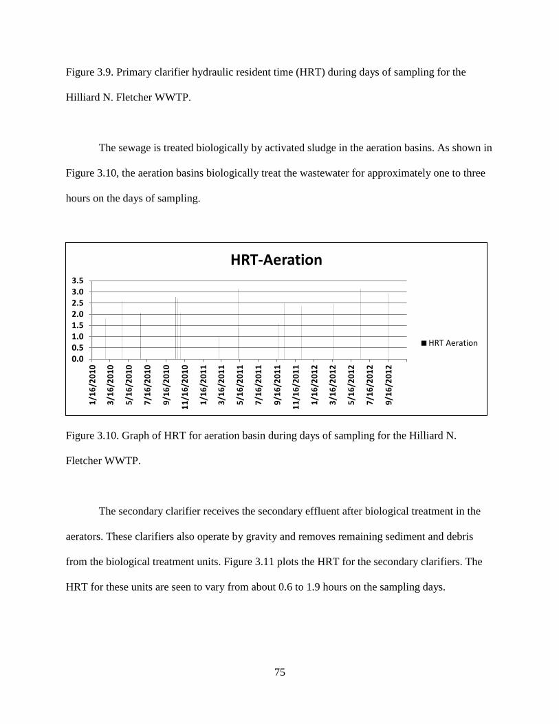
Figure 3.9. Primary clarifier hydraulic resident time (HRT) during days of sampling for the
Hilliard N. Fletcher WWTP.
The sewage is treated biologically by activated sludge in the aeration basins. As shown in
Figure 3.10, the aeration basins biologically treat the wastewater for approximately one to three
hours on the days of sampling.
Figure 3.10. Graph of HRT for aeration basin during days of sampling for the Hilliard N.
Fletcher WWTP.
The secondary clarifier receives the secondary effluent after biological treatment in the
aerators. These clarifiers also operate by gravity and removes remaining sediment and debris
from the biological treatment units. Figure 3.11 plots the HRT for the secondary clarifiers. The
HRT for these units are seen to vary from about 0.6 to 1.9 hours on the sampling days.
0.00.51.01.52.02.53.03.5
1/16
/201
0
3/16
/201
0
5/16
/201
0
7/16
/201
0
9/16
/201
0
11/1
6/20
10
1/16
/201
1
3/16
/201
1
5/16
/201
1
7/16
/201
1
9/16
/201
1
11/1
6/20
11
1/16
/201
2
3/16
/201
2
5/16
/201
2
7/16
/201
2
9/16
/201
2
HRT-Aeration
HRT Aeration
75
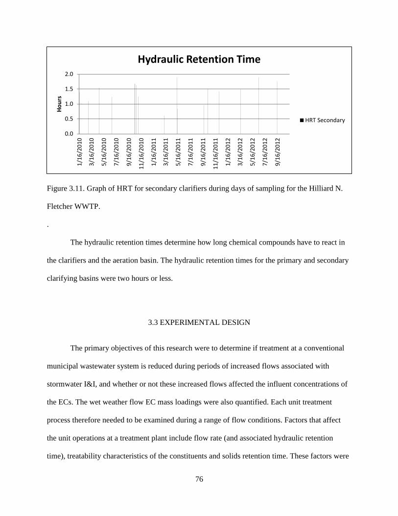
Figure 3.11. Graph of HRT for secondary clarifiers during days of sampling for the Hilliard N.
Fletcher WWTP.
.
The hydraulic retention times determine how long chemical compounds have to react in
the clarifiers and the aeration basin. The hydraulic retention times for the primary and secondary
clarifying basins were two hours or less.
3.3 EXPERIMENTAL DESIGN
The primary objectives of this research were to determine if treatment at a conventional
municipal wastewater system is reduced during periods of increased flows associated with
stormwater I&I, and whether or not these increased flows affected the influent concentrations of
the ECs. The wet weather flow EC mass loadings were also quantified. Each unit treatment
process therefore needed to be examined during a range of flow conditions. Factors that affect
the unit operations at a treatment plant include flow rate (and associated hydraulic retention
time), treatability characteristics of the constituents and solids retention time. These factors were
0.0
0.5
1.0
1.5
2.01/
16/2
010
3/16
/201
0
5/16
/201
0
7/16
/201
0
9/16
/201
0
11/1
6/20
10
1/16
/201
1
3/16
/201
1
5/16
/201
1
7/16
/201
1
9/16
/201
1
11/1
6/20
11
1/16
/201
2
3/16
/201
2
5/16
/201
2
7/16
/201
2
9/16
/201
2
Hour
s Hydraulic Retention Time
HRT Secondary
76

investigated during this research for both dry and wet weather conditions. The constituents
analyzed included:
-Pharmaceuticals
• trimethoprim
• sulfamethoxazole
• fluoxetine
• carbamazepine
• ibuprofen
• gemfibrozil
• triclosan
-Pesticides
• lindane aldrin
• dieldrin
• heptachlor
• heptachlor-epoxide
• methoxychlor
• arochlor
-PAHs
• naphthalene
• phenanthrene
• anthracene
• fluoranthene
• pyrene
• fluorene
• acenaphthene
• chrysene
• Acenaphthylene
77

Eight sets of samples were obtained at the wastewater plant during wet weather and nine
sets of samples were collected during dry weather to compare concentrations and performance as
a function of flow rates.
A total of 24 samples were collected for PAHs, pharmaceuticals and pesticides during
wet weather samples. Twenty-eight samples were collected for PAHs, pharmaceuticals and
pesticides during dry weather conditions. The wet and dry conditions are the causal or
independent variables. This study is designed to measure the effects of wet weather on
wastewater treatment of these ECs. The dependent variables, or the outcome variables, are the
influent and effluent concentrations for each unit process. The wet weather samples were
weather dependent and were therefore obtained as a judgmental sample design (when it was
predicted to have moderate to large amounts of rainfall for the area). The dry weather samples
were taken randomly, increasing variability. Samples were obtained manually as composite grab
samples. All treatment plant samples were taken over a six hour period. Grab samples were
taken at the sampling locations as time composites over a two hour period. The samples were
obtained at: (1) inlet; (2) primary clarifier effluent; (3) secondary clarifier effluent; and (4) after
disinfection at the plant effluent. Each sample was obtained in one liter, pre-washed amber glass
bottles having Teflon-lined lids.
The EPA determined standard analytical processing (storage, extraction, and analysis)
procedures for each category of compound. For the pharmaceuticals evaluated during this study,
EPA method 1694 was used. The pharmaceuticals were held in a cooler at 4 C before extraction.
The pharmaceutical samples were tested for acidic compounds. The method describes the pH
adjustment solutions and extraction solvents to be used: HCl and MeOH. Hydrochloric acid
(HCl) was used to acidify the sample and the methanol (MeOH) was used for extraction. For the
78

analysis, two different elution solvents were used on a solids phase extraction (SPE) setup. One
was used for the first set of four pharmaceuticals: carbamazepine, sulfamethoxazole, fluoxetine,
and trimethoprim. The compounds in the other set were triclosan, gemfibrozil and ibuprofen.
Formic acid (1%) /ammonia formate and formic acid (1%)/in methanol:water was used as the
two extraction solvents. The instrument was calibrated and blanks were analyzed for detection
limits. The final effluent was also spiked to determine extraction recovery efficiency. The
pharmaceuticals were quantified using a HPLC.
For PAHs, the method was EPA method 8310. The initial calibration was conducted
using a minimum blank and 5 points for each analyte. The calibration was verified by internal
calibrations. Method blanks were analyzed for every 20 samples. The PAHs were extracted using
methylene chloride in 2L separation funnels. The extracts were condensed from 120 ml to 2 ml
using Kuderna Danish (KD) equipment. The extract was analyzed using a GC-MS.
The pesticides were sent to Penn State Harrisburg for extractions in a cooler with the
separation funnel extractions completed within the allowable holding time of 7 days. The
pesticides were analyzed using EPA 525 method. Calibration liquids, containing each of the
analytes were prepared. After the samples were collected, they were dechlorinated using sodium
thiosulfate, iced and sent to the lab. Field blanks were analyzed along with samples. QA/QC was
demonstrated by the consistent analysis of laboratory reagent blanks, laboratory fortified blanks
(LFB), and laboratory fortified matrix (LFM) samples. The pesticides were analyzed using a
GC-ECD.
The quality control objective for the laboratory blank is to obtain results in a
concentration less than the specified detection limit. If the blank concentration is greater than the
field samples, the values will be rejected or re-analyzed.
79

3.4 DATA ANALYSES
The data analyses were conducted in several steps. Descriptive statistics were used to illustrate
patterns in the concentrations through the treatment plant, and to present basic statistical
differences. The statistical tests were used to quantify any relationships and differences. The
same sets of plots and statistical tests were repeated for each analyte and are presented in
Appendix A, with summaries in the results and conclusions sections.
3.4.1. Descriptive Statistics
The influent and effluent concentrations for each sample date are graphed as a line graph to
observe concentration changes throughout the treatment plant. Box and whisker plots for each
treatment process also show the variability of concentrations. Probability plots for influent and
effluent sample dates were created to establish normality and to visualize effects of
concentration on treatability. Data series plots also were prepared to compare the influent
concentrations vs. flow to illustrate any trends with weather conditions. Appendix A shows all
statistical analyses for the tested ECs.
3.4.1.1. Statistical tests
Basic statistical tests were conducted to determine if there were significant differences
between influent and effluent for each unit process and overall influent and effluent
concentrations, based on the number of samples obtained and the data variability. In addition,
relationships between influent characteristics and rain conditions were also examined. Basic
statistical summaries of the concentrations and loads are shown in Appendix A (from SigmaPlot
80

ver. 11). Nonparametric Kurskal-Wallis one way ANOVA on ranks (using SigmaPlot ver. 11)
was used to identify if any of the four sampling location groups significantly differed from the
others. SigmaPlot was also used for nonparametric Mann-Whitney rank sum tests comparing
influent vs. primary effluent; primary effluent vs. secondary effluent; secondary effluent vs. final
effluent; and influent vs. effluent. Scatterplots and associated linear regression equations, with
ANOVA analyses of the regressions, were prepared in Excel. The regressions were initially
developed with both an intercept and slope term. The ANOVA calculations identified if the
intercept was significant. If not, the regressions (and ANOVAs) were repeated with the intercept
set to zero, forcing the regression line through the origin. The calculated influent mass values
were evaluated as a function of reported rain depth using the same scatterplot, regression, and
ANOVA procedure.
3.4.1.2 Critical Tests
The Kurskal-Wallis ANOVA tests reveal if there are any differences in the four treatment
processes of the treatment plant. Upon determining if there was a statistically significant
difference, the Mann-Whitney rank sum tests, in conjuction with the plots, were used to identify
which ones were significant. During this dissertation research, comparisons of the concentrations
in each unit process were made between wet weather and dry weather to identify if stormwater
I&I affected the EC treatment,the influent concentrations and the mass loads.
Comparisons of dry and wet weather sample results were conducted using non-
parametric Mann-Whitney rank sum tests. Additional investigations also used combinations of
Pearson correlation, Spearman correlation, and/or covariance tests. The performance of the
treatment plant was examined by investigating the performance for conventional constituents by
81

rain and flow characteristics. Hydraulic residence times in the clarifiers and aeration/activated
sludge tanks determined for the days the samples were collected. This information was
previously noted in the section describing the treatment plant.
82

4.0 RESULTS
Stormwater I&I can have a significant effect on wastewater treatment flow rates (and
pollutant concentrations) and may in turn potentially affect treatment of wastewater pollutants.
The increases of volume during a large rain event may cause a dilution effect for pollutants more
associated with sewage than with stormwater (such as expected for many of the
pharmaceuticals), causing the concentrations to be significantly lower. Lower concentrations of a
pollutant reduce the removal rates of targeted pollutants. However, stormwater I&I can be a
major source of some pollutants entering the treatment plant. As an example, PAHs are more
likely associated with stormwater in urban areas than in separate sanitary wastewater. Increases
of PAHs in wastewater influent during wet weather suggest stormwater is entering the sewer
system. Pesticides are also of interest for this study and are known pollutants associated with
stormwater. Some pharmaceuticals have dual roles in both human and veterinary medicine.
While many would enter the sanitary sewage system from human wastes, pet pharmaceuticals
could enter the system through stormwater contaminated by fecal matter from treated animals.
Samples were collected during a range of flow and rain conditions to understand
whether stormwater contributes ECs to the treatment plant. Mass loads were calculated based
on the measured daily flow rates and the influent concentrations. The mass loads for the dry
weather days were compared to the wet weather day mass loads. The differences were then
related to the rain depth observed for the day to determine if stormwater contribute to the EC
discharges to the treatment plant.
The dissertation hypotheses are:
1. Treatability of emerging contaminants depends on their physical-chemical characteristics,
including concentrations, and the operation of the treatment plant.
83

It is predicted for the first hypothesis that stormwater I&I will increase the concentration of
ECs entering wastewater treatment facilities during wet weather changes due to the exposure to
pollutants from stormwater. Depending on the concentrations and mixtures of ECs in the
influent, treatability may be affected by multiple unit processes.
2. There will be a statistically significant difference in treatability of wastewater during wet
weather compared to dry weather.
Due to stormwater I&I’s contributions to the increases of EC discharges at the treatment
plant, the concentrations during dry weather and wet weather will be significantly different.
Therefore the concentrations will be compared in the wet and the dry weather samples. The
variability of the influent EC concentrations and the primary effluents during wet weather are
expected to be higher than the secondary effluents and the final effluents. However the
treatability may not significantly affect the final effluent quality.
To test the hypothesis, eight dry weather samples were taken in addition to nine wet weather
samples at four locations at the treatment facility. Some of the constituents did not have values
for some of the sample dates and in a few instances, insufficient sample volumes were available
to complete the full suite of analyses. Therefore, the final number of data observations varied.
Each sample set was tested for selected PAHs, pharmaceuticals and pesticides. Daily average
flow rates were obtained from the treatment plant operators and the rainfall data were obtained
from Accu-Weather for the Tuscaloosa Municipal Airport rain gauge.
Table 4.1. Treatment Plant Average Daily Flow Rates and Daily Total Rain Depth on Days of Sampling
84

Weather events for sampling
Tuscaloosa Municipal Airport Total Daily Rainfall (inches)*
Treatment Plant Average Daily Flow Rate (MGD)
01/16/10 (wet) 0.55 18.2 03/02/10 (wet) 0.68 23.3 04/24/10 (wet) 1.01 16.5 06/25/10 (wet) 0.59 20.7 11/02/10 (wet) 0.88 20.5 03/09/11 (wet) 2.67 42.2 05/11/11 (dry) 0 13.5 05/14/11 (dry) 0 30.7 09/20/11 (wet) 0.64 26.5 10/10/11 (dry) 0.07 16.9 03/20/12 (dry) 0 17.1 06/16/12 (dry) 0 13.5 09/15/12 (dry) 0 14.5 11/01/12 (dry) 0 17.1 11/04/12 (dry) 0.05 15.4 11/08/12 (dry) 0 15.9 11/12/12 (wet) 0.44 16.0 * historical rain data obtained from Accu-Weather for the Tuscaloosa Municipal Airport
The average flow during the dry weather sampling days was about 18 MGD, while the
average daily flow during the wet weather sampling days was about 24 MGD. Figure 15 is a box
and whisker plot comparing the dry weather and the wet weather observed flows. Most of the
wet weather flows are larger than the dry weather flows, but there is some overlap (the Mann-
Whitney rank sum test only indicates a marginal significance that they are different at p = 0.07,
likely due to the small number of observations: 6 dry weather samples and 7 wet weather
samples having both rainfall and flow data).
85

Figure 4.1. Treatment plant flows during dry and wet weather.
Figure 4.2 is a plot of these rain depth values compared to the daily average treatment
plant flows (with the zero rain data removed to enable log-transformations). This plot indicates
I&I is not likely significant until the daily rain depth is greater than about one-half inch, when
the treatment plant flow can increase to greater than about 20 MGD. During the largest rain
depth observed (2.67 inches), the treatment plant flow was also the largest observed (42.2
MGD). This plot has a reasonably fit, but it also indicates a large variability. The rain depth is
available only for a single area in the large service area (Tuscaloosa Municipal Airport) and it is
likely that the rains vary greatly over the service area, especially for the smaller rains. In
addition, there are relatively few larger rains compared to the smaller rains, so there is not very
much information available to verify the upper range of this relationship. In addition, elevated
flow rates are also noted during dry weather, which indicates that other factors are involved in
some of the elevated flow rates.
86
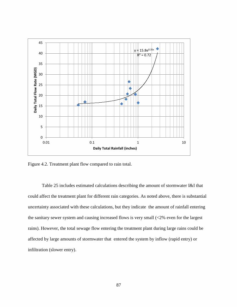
Figure 4.2. Treatment plant flow compared to rain total.
Table 25 includes estimated calculations describing the amount of stormwater I&I that
could affect the treatment plant for different rain categories. As noted above, there is substantial
uncertainty associated with these calculations, but they indicate the amount of rainfall entering
the sanitary sewer system and causing increased flows is very small (<2% even for the largest
rains). However, the total sewage flow entering the treatment plant during large rains could be
affected by large amounts of stormwater that entered the system by inflow (rapid entry) or
infiltration (slower entry).
y = 15.8e0.35x R² = 0.72
0
5
10
15
20
25
30
35
40
45
0.01 0.1 1 10
Daily
Tot
al F
low
Rat
e (M
GD)
Daily Total Rainfall (inches)
87

Table 4.2. Estimated Stormwater Infiltration and Inflow (I&I) for Different Rain Categories
Rain range (in)
Average treatment plant flow (MGD)
Increase over base treatment plant flow assumed due to stormwater I&I (MGD)
Percentage of total treatment plant flow associated with stormwater I&I (%)
Estimated stormwater I&I (MGD/mi2)*
Estimated stormwater I&I (watershed inches)
Estimated stormwater I&I as a percentage of the rain depth (%)
0 to 0.1 17.7 0 0 0 0 0 0.2 to 0.5 18 0.3 2 0.027 0.0015 0.43 0.6 to 1.5 23 5.3 23 0.31 0.018 1.7 1.6 to 2.5 34 16.3 48 0.65 0.037 1.8 * Service area: 74 mi2; the population served: 110,000; the total length of sewers: 600 miles
The mass loads of PAHs and pharmaceuticals during wet weather are compared to the
mass loads during wet weather to determine if there are consistently higher mass loads under wet
weather conditions. Tables 4.3 and 4.4 list calculated influent mass loads for three example
pharmaceuticals during dry and wet weather.
Table 4.3. Influent Mass Load Data for Pharmaceuticals during Dry Weather
Date Rainfall (inches)
Flow rate (MGD)
Ibuprofen (g/day)
Gemfibrozil (g/day)
Triclosan (g/day)
5/11/2011 0.00 13.5 n/a n/a n/a 5/14/2011 0.00 30.7 21,817 37,367 16,130 3/20/2012 0.00 17.1 0 4,266 2,392 6/16/2012 0.00 13.5 0 714 0 9/15/2012 0.00 14.5 0 1,480 0 11/1/2012 0.00 17.1 3,297 5,106 970 11/4/2012 0.05 15.4 0 1,572 0 Average Dry Weather Conditions
0.01 17.4 4,186 8,418 3,249
Table 4.4. Influent Mass Load Data for Pharmaceuticals during Wet Weather
Date Rainfall (inches)
Flow rate (MGD)
Ibuprofen (g/day)
Gemfibrozil (g/day)
Triclosan (g/day)
1/16/2010 0.55 18.2 1,582 688 69 3/2/2010 0.68 23.3 352 1,761 352 4/24/2010 1.01 16.5 1,684 2,807 3,306
88

6/25/2010 0.59 20.7 2,973 2,034 626 11/2/2010 0.88 20.5 2,325 4,649 n/a 3/9/2011 2.67 42.2 <dl 2,712 n/a 9/20/2011 0.64 26.5 <dl 5,409 10,217 Average Wet Weather Conditions
1.00 24.0 1,274 2,866 2,081
There is substantial variability in the mass discharges and the average loads are not
greater during wet weather, as expected. However, regression analyses of influent
concentrations vs. treatment plant flow rate indicated significant slope terms for all three of these
pharmaceutical compounds, as shown in the following figures for triclosan (complete statistical
analyses are presented in Appendix A).
Figure 4.3. Triclosan influent concentrations vs. treatment plant flow rates.
Line graphs showing the concentrations throughout each of the unit processes at the
treatment plant are a visual representation of the treatability of each compound for each unit
process. Dry weather and wet weather sample concentration patterns are compared to represent
the differences in treatment during varied weather conditions. The wet weather samples were
taken during days with anticipated rain, with the total daily rain amounts ranging from 0.05 to
y = 6.9x - 105 R² = 0.59; p = 0.003
0
20
40
60
80
100
120
140
160
0 5 10 15 20 25 30 35
Influ
ent T
riclo
san
(ug/
L)
Treatment Plant Daily Flow Rate (MGD)
89
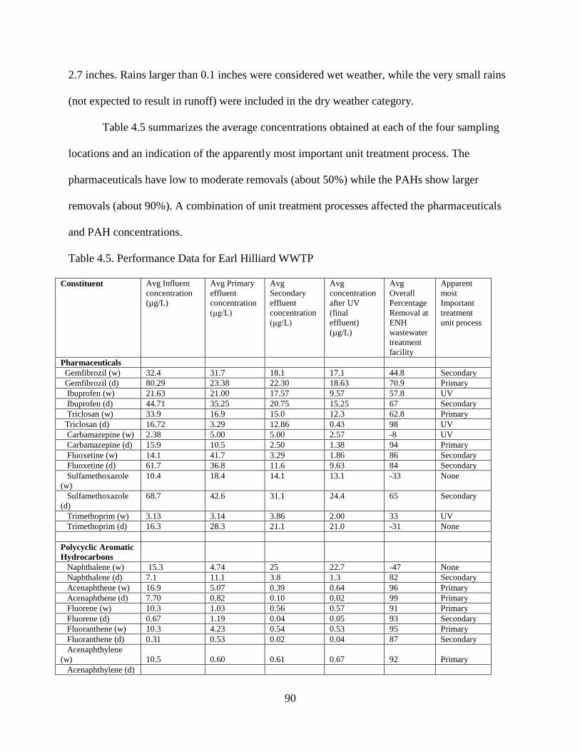
2.7 inches. Rains larger than 0.1 inches were considered wet weather, while the very small rains
(not expected to result in runoff) were included in the dry weather category.
Table 4.5 summarizes the average concentrations obtained at each of the four sampling
locations and an indication of the apparently most important unit treatment process. The
pharmaceuticals have low to moderate removals (about 50%) while the PAHs show larger
removals (about 90%). A combination of unit treatment processes affected the pharmaceuticals
and PAH concentrations.
Table 4.5. Performance Data for Earl Hilliard WWTP
Constituent Avg Influent concentration (µg/L)
Avg Primary effluent concentration (μg/L)
Avg Secondary effluent concentration (μg/L)
Avg concentration after UV (final effluent) (µg/L)
Avg Overall Percentage Removal at ENH wastewater treatment facility
Apparent most Important treatment unit process
Pharmaceuticals Gemfibrozil (w) 32.4 31.7 18.1 17.1 44.8 Secondary Gemfibrozil (d) 80.29 23.38 22.30 18.63 70.9 Primary Ibuprofen (w) 21.63 21.00 17.57 9.57 57.8 UV Ibuprofen (d) 44.71 35.25 20.75 15.25 67 Secondary Triclosan (w) 33.9 16.9 15.0 12.3 62.8 Primary Triclosan (d) 16.72 3.29 12.86 0.43 98 UV Carbamazepine (w) 2.38 5.00 5.00 2.57 -8 UV Carbamazepine (d) 15.9 10.5 2.50 1.38 94 Primary Fluoxetine (w) 14.1 41.7 3.29 1.86 86 Secondary Fluoxetine (d) 61.7 36.8 11.6 9.63 84 Secondary Sulfamethoxazole (w)
10.4 18.4 14.1 13.1 -33 None
Sulfamethoxazole (d)
68.7 42.6 31.1 24.4 65 Secondary
Trimethoprim (w) 3.13 3.14 3.86 2.00 33 UV Trimethoprim (d) 16.3 28.3 21.1 21.0 -31 None Polycyclic Aromatic Hydrocarbons
Naphthalene (w) 15.3 4.74 25 22.7 -47 None Naphthalene (d) 7.1 11.1 3.8 1.3 82 Secondary Acenaphthene (w) 16.9 5.07 0.39 0.64 96 Primary Acenaphthene (d) 7.70 0.82 0.10 0.02 99 Primary Fluorene (w) 10.3 1.03 0.56 0.57 91 Primary Fluorene (d) 0.67 1.19 0.04 0.05 93 Secondary Fluoranthene (w) 10.3 4.23 0.54 0.53 95 Primary Fluoranthene (d) 0.31 0.53 0.02 0.04 87 Secondary Acenaphthylene (w)
10.5
0.60
0.61
0.67
92
Primary
Acenaphthylene (d)
90

0.08 0.58 0.01 0.02 75 Secondary Phenanthrene (w) 6.14 4.36 0.05 0.15 98 Secondary Phenanthrene (d) 1.56 0.77 0.16 0.12 90 Primary and
secondary Anthracene (w) 198 2.27 9.70 0.81 100 Primary Anthracene (d) 60.07 0.18 0.24 0.15 100 Primary Pyrene (w) 10.24 4.04 0.72 0.51 95 Primary and
secondary Pyrene (d) 0.66 0.95 0.13 0.13 80 Secondary
Figure 4.4 is a line-treatability plot for naphthalene for the dry weather events. Each
sample event varies in treatability. Naphthalene appears to have significant removal during
secondary treatment, but with limited removal during both primary sedimentation and the final
disinfection stages.
Figure 4.4. Treatability line plot for naphthalene during dry weather.
Table 4.6 is a summary of the preliminary analyses for semivolatile compounds
(phthaltes and pesticides) detected. Although no statistical anlaysis were conducted on this data,
it is seem that all secondary and final effluent concentrations were below the concentration
0.01
0.1
1
10
100
Influent Primary Secondary Final
Conc
μg/
L
Naphthlene
10/24/2010
5/11/2011
5/14/2011
3/20/2012
91

detection limits, indicating that all of the analytes were removed during secondary treatment. No
pesticides were detrected at the 0.5 to 1 µg/L detection limit.
Table 4.6. Preliminary semivolatile analyses results (phthalate esters and pesticides)
Sample date Influent Primary
Secondary/Final
1/16/2010
Butylbenzylphthalate 11.1 Di-n-Butylphthalate 3.9 Diethylphthalate 12.3 bis(2-Ethylhexyl)phthalate 53.9 Naphthalene 2.0
Butylbenzylphthalate 3.5 Di-n-Butylphthalate 2.7 Diethylphthalate 6.3 bis(2- thylhexyl)phthalate 17.8 Naphthalene 1.0
all ND
3/2/2010
bis(2-Ethylhexyl)phthalate 6.9 2-Methylnaphthalene 2.2 Naphthalene 1.1
bis(2-Ethylhexyl)phthalate 8.6 Fluorene 0.52 2-Methylnaphthalene 2.0 Metribuzin 1.9 Naphthalene 1.1 all ND
4/24/2010 bis(2-Ethylhexyl)phthalate 8.8
bis(2-Ethylhexyl)phthalate 7.1 all ND
6/25/2010
Benzo(a)anthracene 0.63 Butylbenzylphthalate 13.3 Chrysene 0.77 bis(2-Ethylhexyl)phthalate 26.2 Phenanthrene 0.77 Pyrene 0.52
Butylbenzylphthalate 9.0 Di-n-Butylphthalate 2.6 bis(2-Ethylhexyl)phthalate 15.8
all ND all ND (duplicate)
11/2/2010
Butylbenzylphthalate 4.6 Di-n-Butylphthalate 4.5 Diethylphthalate 7.8 bis(2-Ethylhexyl)phthalate 9.6 2-Methylnaphthalene 4.6 Naphthalene 2.5
Butylbenzylphthalate 3.3 Di-n-Butylphthalate 3.2 Diethylphthalate 6.7 bis(2-Ethylhexyl)phthalate 10.4 2-Methylnaphthalene 6.0 Naphthalene 3.7 all ND
3/9/2011 Anthracene 0.54 Fluoranthene 0.57 2-Methylnaphthalene
2-Methylnaphthalene 3.8 Naphthalene 1.9 all ND
92

3.9 Naphthalene 2.0 Phenanthrene 0.87 Pyrene 0.55
Phenanthrene 0.86
93

5.0 CONCLUSIONS
The purpose of this research was to investigate how stormwater affects the treatment of
emerging contaminants at wastewater treatment plants and to determine stormwater contributions
of ECs during wet weather. Influent, primary effluent, secondary effluent and final effluent after
UV disinfection for wet weather and dry weather were compared to identify any significance
differences in treatment for the unit processes during both wet and dry weather conditions.
Physical and chemical properties of each EC constituent were summarized from published
literature, including descriptions how these properties can affect their treatability by different
unit processes. These predictions were compared to the findings during this research to
determine the significance of the chemical properties and the unit processes at the treatment
plant. These preliminary findings are based on results for three pharmaceuticals for which data
are currently available: triclosan, gemfibrozil and ibuprofen.
The dissertation’s hypotheses are below:
1.Treatability of emerging contaminants depends on their physical-chemical
characteristics, including concentrations and the operation of the treatment plant.
Ibuprofen has a pKa value of 4.9. In wastewater consistently having pH values above 6
(and generally close to neutral), ibuprofen is therefore ionized. It has a relatively high solubility
of 41.5 mg/L, and a concurrent high sorption potential (pKa 3.5 to 4.0). The literature review
reported observed removal rates at wastewater treatment plants from 82 to 95 percent, with
resulting effluent quality from 0.02 to 2 µg/L. The literature focuses on biodegradation as the
most common method of removal of ibuprofen because of its concurrent high solubility and
absorption factors. This research found average removal rates of 66 percent for dry weather
samples and 55 percent for wet weather samples, which were less than indicated in the literature.
94

The effluent ibuprofen concentrations ranged from 15 µg/L for the dry weather samples and 10
µg/L for the wet weather samples (substantially larger than the values reported in the literature).
The most apparent treatment unit process for dry weather samples occurred during secondary
treatment, while the final UV disinfection process was highly important for the wet weather
samples, although none of the unit process removals were statistically significant based on the
number of samples available.
Gemfibrozil has a pKa value of 4.7 which makes this chemical ionize in the nearly
neutral wastewater and stormwater aqueous solutions. It has a relatively high solubility of 5.0
mg/L and a log Kow of 4.78. The literature review reported removal rates from 38 to 76 percent
with biodegradation as the primary means of removal. The gemfibrozil wastewater treatment
plant effluent concentrations ranged from 0.4 to 0.8 µg/L. This research measured removal rates
averaging 71 percent during dry weather and 45 percent during wet weather. The gemfibrozil in
the treated effluent ranged from 19.1 to 89.2 µg/L during dry weather and from 17.5 to 33.1 µg.L
during wet weather, which was also substantially larger than reported in the literature. The most
significant removal unit process for the dry weather samples was primary treatment, while
secondary treatment (which utilizes biodegradation) was the most important unit process during
wet weather.
Triclosan has a pKa of 7.8 which under typical neutral wastewater and stormwater
conditions will not ionize in these aqueous solutions. It also is relatively soluble in water (2 to
4.6 mg/L) and has a high log Kow of 4.8-5.4 indicating a high adsorption potential. The literature
review reported triclosan removals from 60 to 75% in wastewater treatment plants; with effluent
concentrations from 0.11 to 0.22 µg/L. Primary removal unit process is reported to be
biodegradation in the secondary phase of wastewater treatment. During this research, the average
95

removal rates during dry weather were found to be about 97 percent with 64 percent removals
during wet weather. Triclosan concentrations in the treated wastewater effluent ranged from 11
to 32 µg/L during dry weather and 2.2 to 28 µg/L during wet weather, also larger than reported
in the literature. The primary removal unit process during dry weather was secondary treatment
(incorporating biodegradation through oxidation) and primary treatment (sedimentation) during
wet weather conditions.
Carbamazepine has a log Kow value of 2.45 and a pKa of 13.9. It is basic compound, so in
wastewater with a neutral pH, it is expected to ionize. The solubility of carbamazepine is 17.7
mg/L. With ionization in wastewater and a relatively high solubility, carbamazepine has a low
probability of being treated through sedimentation. The LC50 of D. magna is greater than 100
mg/L in a 24-hour period (ToxNET). The maximum concentrations in the wastewater treatment
system were much less than the reported LC50 value so toxicity is not expected to have a large
effect on the treatment of carbamazepine. The biological half-life of carbamazepine is 10 to 20
hours, which means it is relatively stable and may be transported through the wastewater
treatment with small reductions. Literature has shown that carbamazepine is resistant to
biodegradation (Zhang 2008). The literature review shows that carbamazepine removal ranges
from 0 to 30%. In our study, wet weather samples and dry weather samples showed
carbamazepine was reduced by 9.6 and 12%, respectively. Our findings are similar to findings
from the literature. The one way ANOVA and rank sum tests show that there were no
statistically significant differences in the treatment of carbamazepine.
Fluoxetine has a log Kow value of 4.05 and a pKa of 7.9. It also has a relatively high
solubility of 38.4 mg/L. Because of its pKa, there is expected to be some protonation in the
wastewater treatment stream. It also has the potential to sorb onto organic particulates. The LC50
96

of P. subcapitata exposed to fluoxetine is 24 μg/L (Brooks et al. 2003, 169-183). The toxicity
value is close to values observed at the treatment plant, indicating potential inhibition. The half-
life of fluoxetine ranges from 24 to 72 hours. The one way ANOVA showed some statistical
differences in the treatment of fluoxetine. After conducting a Mann-Whitney rank sum test, there
was a significant difference noted between the influent and the final effluent concentrations and
between the primary effluent and secondary effluent concentrations. The average wet weather
removal of fluoxetine was 64%, with secondary treatment being the major removal process.
Under dry weather conditions, there were no reductions noted.
Sulfamethoxazole has a log Kow value of 0.9 and a solubility of 600 mg/l. It also has
pKa1 and pKa2 values of 1.7 and 5.6, respectively. It is also classified as a sulfonamide, a
member of the amide groups. Amides are known to be soluble in water. P. subcapitata exposed
to sulfamethoxazole yields an IC50 of 1.5 mg/L, so toxicity will not likely affect the
microorganisms in the secondary treatment phase (Yang et al. 2009, 1201-1208).
Sulfamethoxazole has a half-life of 10 hours (Hazardous Substance Database 2012). The
literature review gives a range of removals from 17 to 66%. The one way ANOVA and Mann-
Whitney rank sum tests indicated that there was not a statistical significant difference in any of
the treatment processes in this study for the number of samples available. The research findings
indicated that the reduction rates for wet and dry weather for sulfamethoxazole were 9.12 and
0.50%, respectively.
Trimethoprim has a log Kow value of 0.79 and a solubility of 400 mg/L. Its pKa is 6.6
which is close in value to the neutral pH of wastewater. Trimethoprim is predicted to be soluble
in water, making it more difficult to treat. The freshwater green alga P. subcapitata has a LC50 of
80.3 to 130 mg/L for trimethoprim and therefore is unlikely affect biological treatability due to
97

toxicity (Yang et al. 2009, 1201-1208). Trimethoprim has a half-life of 8 to 10 hours. The
literature review indicated that trimethoprim has a removal rate of 70 to 75%. The influent
concentrations from the literature ranged from 0.1 μg/L to 0.5 μg/L. The effluent concentrations
from the literature were about 0.1 μg/L. The reported means of treatment for trimethoprim was
through chlorination. The one way ANOVA test shows that there was no statistically significant
difference between each of the treatment processes during this research. Trimethoprim had
reported 11% reductions during wet weather and 6% reductions during dry weather. The
average influent concentrations were 16 μg/L for dry weather and 3.1 μg/L. The average final
effluent concentrations for dry and wet weather samples were 21 and 2.0 μg/L, respectively. The
concentrations in the experimental data were much greater than presented in the literature.
Naphthalene has a log Kow of 3.37 and a solubility of 31.5 mg/L. This compound is a
lower molecular weight PAH, and therefore is less hydrophobic. It is a semivolatile compound,
having a Henry’s Law constant of 4.6 x 10⁻⁴ atm-m3/mol, so it could be partially removed in the
treatment plant through volatilization. If dissolved in the wastewater stream, it would be
removed through biodegradation or oxidation. The removal rates reported in the literature show
low to moderate removal rates, ranging from 31 to 40%. Influent concentrations from the
literature ranged from 0.15 μg/L to 7.3 μg/L. Effluent concentrations from the literature ranged
from 0.09 μg/L to 0.7 μg/L. The one way ANOVA showed there was not a significant difference
when all four sampling locations were compared, but the Mann-Whitney rank sum test showed
that there was a significant difference in the primary and secondary treatment processes. The
experimental results indicated no reductions for the wet weather or dry weather separately. The
average wet weather concentrations ranged from 15 μg/L for the influent to 23 μg/L for the
98

effluent. There was no apparent method of removal based on the experimental data, which differs
from the literature.
Acenaphthene has a log kow of 4.02 and a solubility of 1.93 mg/L, making it more likely
to be associated with the organic particulate materials. It has a Henry’s Law constant of 7.91 x
10-5 atm-m3/mol, so it is not very volatile. From the literature, influent concentrations ranged
from 0.02 to 0.7 μg/L and the effluent concentrations ranged from 0.005 to 0.11 μg/L. Reported
removal rates ranged from 67 to 85% from the literature. The one way ANOVA tests indicated
there were no significant differences between the four treatment locations, and the Mann-
Whitney rank sum tests also indicated there were no statistically significant differences for any
comparison of the treatment plant locations for the number of samples available. The
experimental results show an average 69% percent removal during dry weather and an average
48% removal during wet weather. These reduction rates are similar to literature findings.
Flourene has a log Kow value of 4.12 and solubility between 1.68-1.98 mg/L, making
fluorene less likely to dissolve in water than to associate with organic particulate matter.
Fluorene is predicted to be removed through primary sedimentation, although oxidation is
another means of removal for PAHs. It is a semivolatile compound. From the literature, reported
removal rates ranged from 59 to 68%. The one way ANOVA indicated that there was a
statistically significant difference at the four treatment locations. After doing a Mann-Whitney
rank sum test, it was determined that there was a significant difference between the primary and
secondary treatment locations. Experimental data indicated average 42% removals for dry
weather conditions and a negative removal rate of -3 % for wet weather conditions.
Flouranthene and pyrene have high log Kow values and low solubility rates, so they are
predicted to adsorb onto particulate organic matter. The literature review shows flouranthene and
99

pyrene to have reduction rates ranging from 83 to 88%. The statistical tests of the data from this
research indicated statistically significant differences in the sampling locations for fluoranthene
when comparing the primary and secondary effluent locations, indicating secondary treatment
benefits. The experimental wet weather samples showed an overall 49 % percent removal and
the experimental dry weather showed an average removal rate of 28%. The higher reductions
during wet weather occurred for the primary unit process. During dry weather conditions, the
most important reductions were for secondary treatment.
For pyrene, the statistical analyses indicated statistically significant reductions in the
primary and secondary treatment unit processes. The experimental results showed an average
50% removal rate during wet weather and a 27% removal rate during dry weather.
From these examples, we see that many of the constituents had concentrations that were
not in the same range as reported in the literature. The analytical methods used during this
research were generally less sensitive than the methods reported in much of the literature,
resulting in only the largest values being detected. The removal rates were also generally lower
than the literature reports, especially for the wet weather conditions.
The high variability and low concentrations of the constituents resulted in few significant
differences between wet and dry weather and between unit processes. Literature indicated the
large amount of variability in the treatment of these constituents that indicate that there are other
factors other than physical and chemical properties that affect these compounds.
2. There will be a statistically significant difference in treatability of wastewater during wet
weather compared to dry weather.
100

Previous data from 2005 through 2008 showed poor correlations between rainfall depths
and flow rates. The flow rates had an apparent increase when rainfall exceeded two inches, but
the variation was large. When the flow and rainfall data were compared for the sampling days, a
somewhat clearer relationship was shown. Box and whisker plots compared the flow rates for
rainfall depths for <0.1 inch, 0.1 to 0.55 inch, 0.56 to 1.0 inch and >1.0 inches. Although there
were obvious flow rate increases as the rain depths increased, especially for the larger rains, a
Kurskal-Wallis 1-way ANOVA on ranks did not identify any significant differences between any
of the rain range groups. Again, the range of flow observations, along with the relatively few
observations, hindered this statistical comparison.
Influent concentrations and mass loads for the three pharmaceutical compounds having
complete data sets at this time were also compared. Regressions indicated significant
relationships between concentrations and flow rates, but not for the mass loads versus rain
depths, as shown in Figure 4.4. Mann-Whitney rank sum tests were conducted for each
constituent comparing influent and effluent concentrations for each unit process and for the
overall influent and effluent concentrations. For the ECs, only gemfibrozil and fluoxetine
showed significant differences between the influent and the final effluent, and no unit process
alone indicated significant concentration differences. In addition, Kurskal-Wallis one way
ANOVAs showed no statistical differences between any of the unit processes for these three
analytes. For the PAHs, acenaphthene, phenanthrene, fluorene, fluoranthene, and pyrene showed
significant differences in the influent and the final concentrations, and also in the secondary and
final treatment locations. Secondary treatment is an important treatment mechanism for PAHs
according to our findings.
101
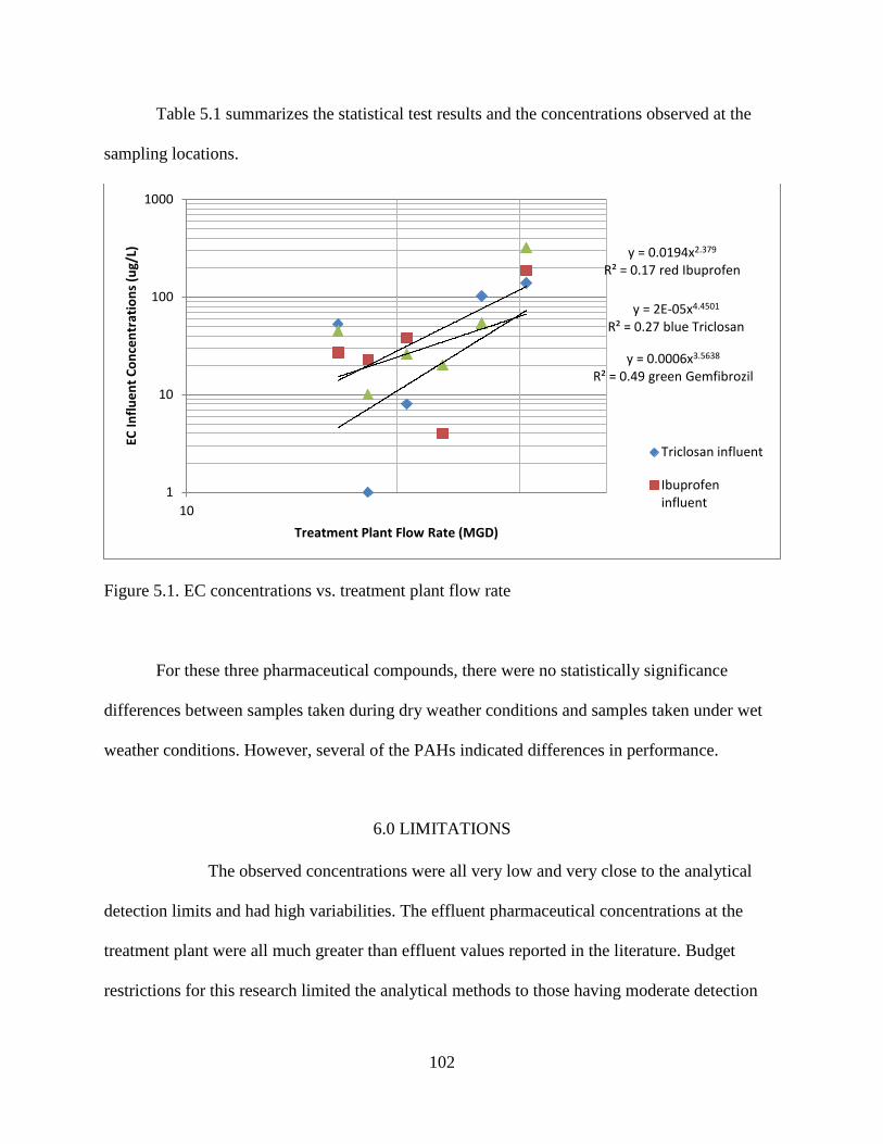
Table 5.1 summarizes the statistical test results and the concentrations observed at the
sampling locations.
Figure 5.1. EC concentrations vs. treatment plant flow rate
For these three pharmaceutical compounds, there were no statistically significance
differences between samples taken during dry weather conditions and samples taken under wet
weather conditions. However, several of the PAHs indicated differences in performance.
6.0 LIMITATIONS
The observed concentrations were all very low and very close to the analytical
detection limits and had high variabilities. The effluent pharmaceutical concentrations at the
treatment plant were all much greater than effluent values reported in the literature. Budget
restrictions for this research limited the analytical methods to those having moderate detection
y = 2E-05x4.4501 R² = 0.27 blue Triclosan
y = 0.0194x2.379 R² = 0.17 red Ibuprofen
y = 0.0006x3.5638 R² = 0.49 green Gemfibrozil
1
10
100
1000
10
EC In
fluen
t Con
cent
ratio
ns (u
g/L)
Treatment Plant Flow Rate (MGD)
Triclosan influent
Ibuprofeninfluent
102

limits, not the ultra-low detection limits sometimes used in reported literature sources. This
resulted in many non-detected observations that were not quantified at the effluent.
The box and whisker plots for the flow rates from 2010 to 2012 indicated statistically
significant differences for three different rainfall categories. However, as to be expected,
monitoring during large rains was not common, with most of the samples collected during the
more likely smaller events that did not produce significant stormwater I&I. The numbers of
samples collected were also limited by the continued dry weather during most of the sampling
period.
The wastewater treatment plant also receives industrial influent from eight different
companies, as described previously (including a commercial laundry and petrochemical service
company, amongst others, that may contribute personal care products and PAHs, respectively, to
the wastewater). Some of these companies discharge large volumes of effluent and can make up
a large portion of the total flow entering the Tuscaloosa treatment plant. These industrial flows
(pre-treated) also likely add to the variability of the treatment plant flows and characteristics.
103

Table 5.1. Summary Statistical Test Results for Selected ECs Examined during this Research
Constituent
Influent (avg. µg/L)
Effluent (avg. µg/L)
p that influent ≠ primary effluent
p that primary effluent ≠ secondary effluent
p that secondary effluent ≠ final effluent
p that influent ≠final effluent
Overall reduction (based on avg. conc., %
Dry weather influent mass (avg. g/day)
Wet weather influent mass (avg. g/day)
p that dry weather influent mass ≠ wet weather influent mass
Wet weather increased conc., from sign. regression slope term (avg. µg/L increase per MGD increase; p of slope term)
Pharmaceuticals Gemfibrozil 59 18 0.14 0.76 0.68 0.04 69% 8,418 2,866 0.67 2.8 (p = 0.01) Ibuprofen 28 15 0.51 0.48 0.40 0.64 46% 4,186 1,274 0.90 6.7 (p = 0.02) Triclosan 28 6.8 0.57 0.92 0.79 0.27 76% 3,249 2,428 0.66 6.9 (p = 0.003) Carbamazepine 8.6 1.9 0.32 0.98 0.74 0.44 11% 953 160 Not calculated Not calculated Fluoxetine 36 6 0.77 0.013 0.42 0.004 27% 4,941 4,046 Not calculated Not calculated Sulfamethoxazole 38 19 0.17 0.90 0.63 0.15 4.8 % 6,096 927 Not calculated Not calculated Trimethoprim 9.3 12.1 0.58 0.96 0.80 0.70 8.4 % 998 275 Not calculated Not calculated Not calculated Not calculated Polycyclic Aromatic Hydrocarbons
Not calculated Not calculated
Naphthalene 11 11 0.90 0.04 0.74 0.08 none 491 1,077 Not calculated Not calculated Acenaphthene 11 0.30 0.11 0.003 1.00 <0.001 75% 483 957 Not calculated Not calculated Fluorene 4.7 0.2 0.65 0.04 0.70 0.04 19% 39 463 Not calculated Not calculated Fluoranthene 4.6 0.27 0.83 0.011 0.75 0.04 38% 19 460 Not calculated Not calculated Acenaphthylene 4.9 0.32 0.61 0.13 0.72 0.06 28% 3.7 484 Not calculated Not calculated Phenanthrene 3.4 0.1 0.70 0.008 0.90 0.011 50% 75 63 Not calculated Not calculated Anthracene 119 0.4 0.17 0.86 0.47 0.069 none 3,235 8,865 Not calculated Not calculated Pyrene 4.8 0.3 0.89 0.021 1.00 0.045 38% 32 458 Not calculated Not calculated
104

REFERENCES
Accinelli, C., W. C. Koskinen, J. M. Becker, and M. J. Sadowsky. 2007. Environmental fate of two sulfonamide antimicrobial agents in soil. Journal of Agricultural and Food Chemistry 55 (7): 2677-82.
AHMAD, TANWEER, MOHD RAFATULLAH, ARNIZA GHAZALI, OTHMAN SULAIMAN, ROKIAH HASHIM, and ANEES AHMAD. 2010. Removal of pesticides from water and wastewater by different adsorbents: A review. Journal of Environmental Science & Health, Part C -- Environmental Carcinogenesis & Ecotoxicology Reviews 28 (4) (Oct): 231-71, http://search.ebscohost.com/login.aspx?direct=true&db=aph&AN=55116096&site=eds-live&scope=site.
Alabama Department of Environmental Management. National pollutant discharge elimination system permit. 2010 [cited September 20 2012]. Available from http://www.adem.state.al.us.
Anderson, Henrik, Hansruedi Siegrist, Bent Halling Sorensen, and Thomas A. Ternes. 2003. Fate of estrogens in a municipal sewage treatment plant. Environmental Science and Technology 37 (18): 4021-4026.
Araujo, L., N. Villa, N. Camargo, M. Bustos, T. García, and A. J. Prieto. 2011. Persistence of gemfibrozil, naproxen and mefenamic acid in natural waters. Environmental Chemistry Letters 9 (1): 13-8.
ATSDR 2011. Toxicological profile of polyaromic hydrocarbona. 2011 [cited April 12 2012]. Available from www.atsdr.gov.
Profile for arochlor. available from. http://www.atsdr.cdc.gov/
Profile for heptachlor. Available from http://www.atsdr.cdc.gov/.
Profile for lindane. cAvailable from http://www.atsdr.cdc.gov.
Profile for methoxychlor. dAvailable from http://www.atsdr.cdc.gov/.
Badawy, MI, M. Y. Ghaly, and T. A. Gad-Allah. 2006. Advanced oxidation processes for the removal of organophosphorus pesticides from wastewater. Desalination 194 (1-3): 166-75.
Beausse, J. 2004. Selected drugs in solid matrices: A review of environmental determination, occurrence and properties of principal substances. TrAC Trends in Analytical Chemistry 23 (10-11): 753-61.
105

Bedner, M., and W. A. MacCrehan. 2006. Reactions of the amine-containing drugs fluoxetine and metoprolol during chlorination and dechlorination processes used in wastewater treatment. Chemosphere 65 (11): 2130-7.
Blanchard, M., M. J. Teil, D. Ollivon, B. Garban, C. Chestérikoff, and M. Chevreuil. 2001. Origin and distribution of polyaromatic hydrocarbons and polychlorobiphenyls in urban effluents to wastewater treatment plants of the paris area (france). Water Research 35 (15): 3679-87.
Blanchard, M., MJ Teil, D. Ollivon, L. Legenti, and M. Chevreuil. 2004. Polycyclic aromatic hydrocarbons and polychlorobiphenyls in wastewaters and sewage sludges from the paris area (france). Environmental Research 95 (2): 184-97.
Bolong, N., A. F. Ismail, M. R. Salim, and T. Matsuura. 2009. A review of the effects of emerging contaminants in wastewater and options for their removal. Desalination 239 (1-3) (4): 229-46.
Bondy, GS, WH Newsome, CL Armstrong, CAM Suzuki, J. Doucet, S. Fernie, SL Hierlihy, MM Feeley, and MG Barker. 2000. Trans-nonachlor and cis-nonachlor toxicity in sprague-dawley rats: Comparison with technical chlordane. Toxicological Sciences 58 (2): 386-98.
Bonefeld-Jørgensen, E. C., H. R. Andersen, T. H. Rasmussen, and A. M. Vinggaard. 2001. Effect of highly bioaccumulated polychlorinated biphenyl congeners on estrogen and androgen receptor activity. Toxicology 158 (3): 141-53.
Boyd, G. R., H. Reemtsma, D. A. Grimm, and S. Mitra. 2003. Pharmaceuticals and personal care products (PPCPs) in surface and treated waters of louisiana, USA and ontario, canada. The Science of the Total Environment 311 (1-3): 135-49.
Brooks, B. W., C. M. Foran, S. M. Richards, J. Weston, P. K. Turner, J. K. Stanley, K. R. Solomon, M. Slattery, and T. W. La Point. 2003. Aquatic ecotoxicology of fluoxetine. Toxicology Letters 142 (3): 169-83.
Busetti, F., A. Heitz, M. Cuomo, S. Badoer, and P. Traverso. 2006. Determination of sixteen polycyclic aromatic hydrocarbons in aqueous and solid samples from an italian wastewater treatment plant. Journal of Chromatography A 1102 (1-2): 104-15.
Campbell, Chris G., Sharon E. Borglin, F. Bailey Green, Allen Grayson, Eleanor Wozei, and William T. Stringfellow. 2006. Biologically directed environmental monitoring, fate, and transport of estrogenic endocrine dsirupting compounds in water: A review. Chemosphere(66): 1265-1280.
Carballa, M., F. Omil, J. M. Lema, M. Llompart, C. Garcia-Jares, I. Rodríguez, M. Gómez, and T. Ternes. 2004. Behavior of pharmaceuticals, cosmetics and hormones in a sewage treatment plant. Water Research 38 (12): 2918-26.
106

Castiglioni, S., R. Bagnati, R. Fanelli, F. Pomati, D. Calamari, and E. Zuccato. 2006. Removal of pharmaceuticals in sewage treatment plants in italy. Environmental Science & Technology 40 (1): 357-63.
Chen, X., J. L. Nielsen, K. Furgal, Y. Liu, I. B. Lolas, and K. Bester. 2011. Biodegradation of triclosan and formation of methyl-triclosan in activated sludge under aerobic conditions. Chemosphere 84 (4): 452-6.
Cherednichenko, G., R. Zhang, R. A. Bannister, V. Timofeyev, N. Li, E. B. Fritsch, W. Feng, G. C. Barrientos, N. H. Schebb, and B. D. Hammock. 2012. Triclosan impairs excitation–contraction coupling and Ca2 dynamics in striated muscle. Proceedings of the National Academy of Sciences 109 (35): 14158-63.
Cleuvers, M. 2003. Aquatic ecotoxicity of pharmaceuticals including the assessment of combination effects. Toxicology Letters 142 (3): 185-94.
Crunkilton, R. L., and W. M. DeVita. 1997. Determination of aqueous concentrations of polycyclic aromatic hydrocarbons (PAHs) in an urban stream. Chemosphere 35 (7): 1447-63.
Dabestani, Reza, and Ilia N. Ivanov. 1999. A compilation of physical, spectroscopic and photophysical properties of polycyclic aromatic hydrocarbons. Photochemistry and Photobiology 70 (1): 10-34.
DrugBank. Open data drug and drug target database. 2012 [cited December 15 2012]. Available from http://www.drugbank.ca/.
Göbel, Anke, Christa S. McArdell, Adriano Joss, Hansruedi Siegrist, and Walter Giger. 2007. Fate of sulfonamides, macrolides, and trimethoprim in different wastewater treatment technologies. Science of the Total Environment 372 (2-3) (1/1): 361-71.
Hazardous Substance Database. TOXNET-toxicology data network. 2012 [cited December 15 2012]. Available from http://toxnet.nlm.nih.gov/cgi-bin/sis/htmlgen?HSDB.
Heberer, Thomas. 2002. Occurrence, fate, and removal of pharmaceutical residues in the aquatic environment: A review of recent research data. Toxicology Letters 131 (1–2) (5/10): 5-17.
Heidler, Jochen, and Rolf U. Halden. 2007. Mass balance assessment of triclosan removal during conventional sewage treatment. Chemosphere 66 : 362-369.
International Labour Organisation, United Nations Environment Programme, and World Health Organization. 1988. International programme on chemical safety (IPCS)United Nations Environment Programme.
107

Jiries, Anwar, Farh M. Al-Nasir, and Friedrich Beese. 2002. Pesticide and heavy metal residue in wastewater, soil and plants in wastewater disposal site near al-lajoun valley, Karak/Jordan. Water, Air and Soil Pollution(133): 97-107.
Joss, Adriano, Elvira Keller, Alfredo C. Alder, Anke Göbel, Christa S. McArdell, Thomas Ternes, and Hansruedi Siegrist. 2005. Removal of pharmaceuticals and fragrances in biological wastewater treatment. Water Research 39 (14) (9): 3139-52.
Kafi, M., J. Gasperi, R. Moilleron, MC Gromaire, and G. Chebbo. 2008. Spatial variability of the characteristics of combined wet weather pollutant loads in paris. Water Research 42 (3): 539-49.
Kahle, Maren, Ignaz Buerge, Andrea Hauser, Markus D. Muller, and Thomas Poigner. 2008. Azole fungicides: Occurrence and fate in wastewater and surface water. Environmental Science and Technology(42): 7193-7200.
Katsoyiannis, A., and C. Samara. 2004. Persistent organic pollutants (POPs) in the sewage treatment plant of thessaloniki, northern greece: Occurrence and removal. Water Research 38 (11): 2685-98.
Kawano, M., T. Inoue, T. Wada, H. Hidaka, and R. Tatsukawa. 1988. Bioconcentration and residue patterns of chlordane compounds in marine animals: Invertebrates, fish, mammals, and seabirds. Environmental Science & Technology 22 (7): 792-7.
Kim, Y., K. Choi, J. Jung, S. Park, P. G. Kim, and J. Park. 2007. Aquatic toxicity of acetaminophen, carbamazepine, cimetidine, diltiazem and six major sulfonamides, and their potential ecological risks in korea. Environment International 33 (3): 370-5.
Kolpin, Dana W., Edward T. Furlong, Michael T. Meyer, Michael E. Thurman, Steven D. Zaugg, Larry B. Barber, and Herbert T. Buxton. 2002. Pharmaceuticals, hormones, and other organic wastewater contaminants in U.S. streams, 1999-2000: A national reconnaissance. Environmental Science and Technology 36 : 1202-1211.
Latch, D. E., J. L. Packer, B. L. Stender, J. VanOverbeke, W. A. Arnold, and K. McNeill. 2005. Aqueous photochemistry of triclosan: Formation of 2, 4‐dichlorophenol, 2, 8‐dichlorodibenzo‐p‐dioxin, and oligomerization products. Environmental Toxicology and Chemistry 24 (3): 517-25.
Lindqvist, Niina, Tuula Tuhkanen, and Leif Kronberg. 2005. Occurrence of acidic pharmaceuticals in raw and treated sewages and in receiving waters. Water Research 39 (11) (6): 2219-28.
Lishman, L., S. A. Smyth, K. Sarafin, S. Kleywegt, J. Toito, T. Peart, B. Lee, M. Servos, M. Beland, and P. Seto. 2006. Occurrence and reductions of pharmaceuticals and personal care products and estrogens by municipal wastewater treatment plants in ontario, canada. Science of the Total Environment 367 (2-3): 544-58.
108

Manoli, E., and C. Samara. 1999. Occurrence and mass balance of polycyclic aromatic hydrocarbons in the thessaloniki sewage treatment plant. Journal of Environmental Quality 28 (1): 176-86.
Mauricio, R., M. Diniz, Mira Petrovic, L. Amaral, I. Peres, Damia Barcelo, and F. Santana. 2006. A characterization of selected endocrine disruptor compounds in a portuguese wastewater treatment plant. Environmental Monitoring and Asessment(118): 75-87.
Miao, X. S., F. Bishay, M. Chen, and C. D. Metcalfe. 2004. Occurrence of antimicrobials in the final effluents of wastewater treatment plants in canada. Environmental Science & Technology 38 (13): 3533-41.
Miao, X. S., J. J. Yang, and C. D. Metcalfe. 2005. Carbamazepine and its metabolites in wastewater and in biosolids in a municipal wastewater treatment plant. Environmental Science & Technology 39 (19): 7469-75.
Miege, C., JM Choubert, L. Ribeiro, M. Eusebe, and M. Coquery. 2009. Fate of pharmaceuticals and personal care products in wastewater treatment plants-conception of a database and first results. Environmental Pollution 157 (5): 1721-6.
Mikes, O., and S. Trapp. 2010. Acute toxicity of the dissociating veterinary antibiotics trimethoprim to willow trees at varying pH. Bulletin of Environmental Contamination and Toxicology: 1-6.
Mohapatra, DP, SK Brar, RD Tyagi, and RY Surampalli. 2010. Physico-chemical pre-treatment and biotransformation of wastewater and wastewater sludge-fate of bisphenol A. Chemosphere 78 (8): 923-41.
Monteith, H. D., W. J. Parker, J. P. Bell, and H. Melcer. 1995. Modeling the fate of pesticides in municipal wastewater treatment. Water Environment Research 67 (6) (Sep. - Oct.): pp. 964-970, http://www.jstor.org/stable/25044650.
Myers, R. C. 2009. Modeling the Fate of Emerging Contaminants and Investigating the Importance of their Physical, Chemical, and Biological Properties in Water and Wastewater Treatment. A Dissertation
Nakada, Norihide, Toshikatsu Tanishima, Hiroyuki Shinohara, Kentaro Kiri, and Hideshige Takada. 2006. Pharmaceutical chemicals and endocrine disrupters in municipal wastewater in tokyo and their removal during activated sludge treatment. Water Research 40 (17) (10): 3297-303.
Nentwig, G. 2007. Effects of pharmaceuticals on aquatic invertebrates. part II: The antidepressant drug fluoxetine. Archives of Environmental Contamination and Toxicology 52 (2): 163-70.
109
Nghiem, L. D., A. I. Schäfer, and M. Elimelech. 2005. Pharmaceutical retention mechanisms by nanofiltration membranes. Environmental Science & Technology 39 (19): 7698-705.
Pérez, S., P. Eichhorn, and D. S. Aga. 2009. Evaluating the biodegradability of sulfamethazine, sulfamethoxazole, sulfathiazole, and trimethoprim at different stages of sewage treatment. Environmental Toxicology and Chemistry 24 (6): 1361-7.
Petrovic, M., S. Gonzalez, and D. Barceló. 2003. Analysis and removal of emerging contaminants in wastewater and drinking water. TrAC Trends in Analytical Chemistry 22 (10): 685-96.
Petrovic, M., M. Gros, and D. Barcelo. 2006. Multi-residue analysis of pharmaceuticals in wastewater by ultra-performance liquid chromatography-quadrupole-time-of-flight mass spectrometry. Journal of Chromatography A 1124 (1-2): 68-81.
Pham, T. T., and S. Proulx. 1997. PCBs and PAHs in the montreal urban community (quebec, canada) wastewater treatment plant and in the effluent plume in the st lawrence river. Water Research 31 (8): 1887-96.
Phillips, P. J., and A. Chalmers. 2009. Wastewater effluent, combined sewer overflows, and other sources of organic compounds to lake champlain. Journal of the American Water Resources Association 45 (1): 45-57.
Phillips, PJ, B. Stinson, SD Zaugg, ET Furlong, DW Kolpin, KM Esposito, B. Bodniewicz, R. Pape, and J. Anderson. 2005. A Multi-disciplinary Approach to the Removal of Emerging Contaminant in Municipal Wastewater Treatment Plants in New York State, 2003-2004. Proceedings of the Water Environment Federation 2005 (10): 5095-124.
PubMed Molecular Biology Database. Available from http://toxnet.nlm.nih.gov/cgi-bin/sis/search/f?./temp/~23N7w0:1:fate.
Radjenovic, J., M. Petrovic, and D. Barceló. 2007. Analysis of pharmaceuticals in wastewater and removal using a membrane bioreactor. Analytical and Bioanalytical Chemistry 387 (4): 1365-77.
Rosal, Roberto, Antonio Rodríguez, José Antonio Perdigón-Melón, Alice Petre, Eloy García-Calvo, María José Gómez, Ana Agüera, and Amadeo R. Fernández-Alba. 2010. Occurrence of emerging pollutants in urban wastewater and their removal through biological treatment followed by ozonation. Water Research 44 (2) (1): 578-88.
Saleh, Farida Y., G. Fred Lee, and Harold W. Wolf. 1980. Selected organic pesticides, occurrence, transformation and removal from wastewater. Journal WPCF 52 (1): 19-28.
Sellin, M. K., D. D. Snow, D. L. Akerly, and A. S. Kolok. 2009. Estrogenic compounds downstream from three small cities in eastern nebraska: Occurrence and biological Effect1. JAWRA Journal of the American Water Resources Association 45 (1): 14-21.
110

Sethia, S., and E. Squillante. 2004. Solid dispersion of carbamazepine in PVP K30 by conventional solvent evaporation and supercritical methods. International Journal of Pharmaceutics 272 (1-2): 1-10.
Singer, H., S. Müller, C. Tixier, and L. Pillonel. 2002. Triclosan: Occurrence and fate of a widely used biocide in the aquatic environment: Field measurements in wastewater treatment plants, surface waters, and lake sediments. Environmental Science & Technology 36 (23): 4998-5004.
Snyder, S., E. Wert, P. Westerhoff, Y. Yoon, D. Rexing, and R. Zegers. 2006. Occurrence and treatment of endocrine disruptors and pharmaceuticals. Paper presented at Proceedings, the 12th Canadian National Conference & 3rd Policy Forum on Drinking Water, Saint John, New Brunswick, .
Stephen Chapman, C. H. M., and I. Law. Membrane bioreactors (MBR) for municipal wastewater Treatment–An australian perspective.
Ternes, Thomas A. 1998. Occurrence of drugs in german sewage treatment plants and rivers. Water Research 32 (11) (11): 3245-60.
Teske, Sondra A., and Robert G. Arnold. 2008. Removal of natural and xenoestrogens during conventional wastewater treatment. Rev Environ Sci Biotechnol(7): 107-124.
U.S Census 2010. 2010 [cited November 30 2010]. Available from http://quickfacts.census.gov/qfd/states/01/0177256.html.
U.S. Environmental Protection Agency. Revised environmental fate science chapter for the triclosan reregistration eligibility decision (RED) document. 2008 [cited December 24 2012]. Available from www.epa.gov (accessed December 24 2012).
"Toxicological review of chlordane (technical)". CAS no. 12789-03-6. in US EPA [database online]. [cited April 15 2012]. Available from http://www.epa.gov/iris/toxreviews/0142tr.pdf.
U.S. EPA 2001. Lindane(gamma-hexachlorocyclohexane). [cited 2001 Available from http://www.epa.gov/ttn/atw/hlthef/lindane.html.
Walker, K., D. A. Vallero, and R. G. Lewis. 1999. Factors influencing the distribution of lindane and other hexachlorocyclohexanes in the environment. Environmental Science & Technology 33 (24): 4373-8.
Weyrauch, P., A. Matzinger, E. Pawlowsky-Reusing, S. Plume, D. von Seggern, B. Heinzmann, K. Schroeder, and P. Rouault. 2010. Contribution of combined sewer overflows to trace contaminant loads in urban streams. Water Research 44 (15): 4451-62.
Williams, J. Endocrine disruptors in wastewater.
111

Xu, B., D. Mao, Y. Luo, and L. Xu. 2011. Sulfamethoxazole biodegradation and biotransformation in the water–sediment system of a natural river. Bioresource Technology 102 (14): 7069-76.
Xu, Weihai, Gan Zhang, Xiangdong Li, Shichun Zou, Ping Li, Zhaohui Hu, and Jun Li. 2007. Occurrence and elimination of antibiotics at four sewage treatment plants in the pearl river delta (PRD), south china. Water Research 41 (19) (11): 4526-34.
Yang, L. H., G. G. Ying, H. C. Su, J. L. Stauber, M. S. Adams, and M. T. Binet. 2009. Growth‐inhibiting effects of 12 antibacterial agents and their mixtures on the freshwater microalga pseudokirchneriella subcapitata. Environmental Toxicology and Chemistry 27 (5): 1201-8.
Zhang, Yongjun, Sven-Uwe Geißen, and Carmen Gal. 2008. Carbamazepine and diclofenac: Removal in wastewater treatment plants and occurrence in water bodies. Chemosphere 73 (8) (11): 1151-61.
112

APPENDIX A: DETAILED OBSERVATIONS
A.1 Pharmaceuticals A.1.1. Summary Data for Gemfibrozil Influent
(µg/L) After Primary (µg/L)
After Secondary (µg/L)
Final Effluent (µg/L)
Daily Flow (MGD)
Mass Influent (g/day)
Daily Rain Depth at Tuscaloosa airport (in)
Overall % Reduction
1/16/2010 10 9.0 <dl <dl 18.2 688 0.55 100 3/2/2010 20 40 33 35 23.3 1,761 0.68 -75 4/24/2010 45 n/a n/a n/a 16.5 2,807 1.01 n/a 6/25/2010 26 23 <dl 15 20.7 2,034 0.59 42 11/2/2010 60 16 19 19 20.5 4,649 0.88 68 3/9/2011 17 12 14 <dl 42.2 2,712 2.67 100 5/11/2011 n/a 30 45 40 13.5 n/a 0.00 n/a 5/14/2011 322 39 38 35 30.7 37,367 0.00 89 9/20/2011 54 77 47 36 26.5 5,409 0.64 33 3/20/2012 66 70 35 37 17.1 4,266 0.00 44 6/16/2012 14 <dl 16 <dl 13.5 714 0.00 100 9/15/2012 27 <dl <dl 22 14.5 1,480 0.00 19 11/1/2012 79 21 1.4 <dl 17.1 5,106 0.00 100 11/4/2012 27 14 29 <dl 15.4 1,572 0.05 100 Average dry (<0.1 inch of rain)
89 25 24 19 17.4 8,418 0.01
79 (calc. from averages)
Average wet 33 30 19 18 24 2,866 1.00 45 (calc. from averages)
* insufficient sample volume for analyses
113

Figure A.1.1.1 Probability plot for Gemfibrozil
4002000-200
99
90
50
10
1100500-50
99
90
50
10
1
500-50
99
90
50
10
1500-50
99
90
50
10
1
Influent3
Perc
ent
Primary3
Secondary3 Final3
Mean 53.67StDev 86.95N 12AD 2.252P-Value <0.005
Influent3
Mean 26.75StDev 27.03N 12AD 0.632P-Value 0.075
Primary3
Mean 19.17StDev 15.85N 12AD 0.469P-Value 0.202
Secondary3
Mean 17.83StDev 15.35N 12
Final3
Normal - 95% CIProbability Plot of Gemfibrozil
114

Figure A.1.1.2 Line graph of Gemfibrozil at four sampling locations Column Size Missing Mean Std Dev Std. Error C.I. of Mean Influent 15 2 59.000 82.000 22.743 49.552 after primary 15 2 27.000 24.187 6.708 14.616 after secondary 15 2 21.338 17.627 4.889 10.652 final effluent 15 2 18.385 16.810 4.662 10.158 FlowMGD 10 0 22.900 8.462 2.676 6.053 mass 9 1 7178.456 12293.197 4346.301 10277.369 rain depth 15 0 0.476 0.710 0.183 0.393 Column Range Max Min Median 25% 75% Influent 312.000 322.000 10.000 27.000 19.250 61.500 after primary 77.000 77.000 0.000 21.000 11.250 39.250 after secondary 47.000 47.000 0.000 19.000 1.050 35.750 final effluent 40.000 40.000 0.000 19.000 0.000 35.250 FlowMGD 28.700 42.200 13.500 20.600 16.900 26.500
0.1
1
10
100
1000
Influent Primary Secondary Final
conc
(μg/
L)
Gemfibrozil
01/16/10 (w)
03/02/10 (w)
04/24/10 (w)
06/25/10 (w)
11/02/10 (w)
03/09/11 (w)
05/11/11 (d)
05/14/11 (d)
09/20/11 (w)
03/20/12 (d)
06/16/12 (d)
09/15/12 (d)
11/01/12 (d)
11/04/12 (d)
11/08/12 (d)
11/12/12 (w)
MDL (upper)
MDL (lower)
115

mass 36678.852 37366.812 687.960 2759.211 1897.938 5029.290 rain depth 2.670 2.670 0.000 0.0700 0.000 0.670 Column Skewness Kurtosis K-S Dist. K-S Prob. SWilk W SWilk Prob Influent 3.171 10.720 0.327 <0.001 0.554 <0.001 after primary 1.086 0.497 0.181 0.278 0.884 0.080 after secondary 0.0310 -1.550 0.179 0.295 0.897 0.123 final effluent 0.00268 -1.927 0.248 0.028 0.817 0.011 FlowMGD 1.438 2.213 0.203 0.279 0.881 0.134 mass 2.743 7.631 0.432 <0.001 0.536 <0.001 rain depth 2.305 6.466 0.251 0.012 0.696 <0.001
Figure A.1.1.3 Box and Whisker plots for Gemfibrozil Normality Test (Shapiro-Wilk) Failed (P < 0.050) Kruskal-Wallis One Way Analysis of Variance on Ranks Group N Missing Median 25% 75% Influent 15 2 27.000 18.500 63.000 after primary 15 2 21.000 10.500 39.500 after secondary 15 2 19.000 0.700 36.500 final effluent 15 2 19.000 0.000 35.500 H = 5.408 with 3 degrees of freedom. (P = 0.144) The differences in the median values among the treatment groups are not great enough to exclude the possibility that the difference is due to random sampling variability; there is not a statistically significant difference (P = 0.144)
116

Mann-Whitney Rank Sum Test Normality Test (Shapiro-Wilk) Failed (P < 0.050) Group N Missing Median 25% 75% Influent 15 2 27.000 18.500 63.000 after primary 15 2 21.000 10.500 39.500 Mann-Whitney U Statistic= 55.500 T = 204.500 n(small)= 13 n(big)= 13 (P = 0.144) The difference in the median values between the two groups is not great enough to exclude the possibility that the difference is due to random sampling variability; there is not a statistically significant difference (P = 0.144) Mann-Whitney Rank Sum Test Normality Test (Shapiro-Wilk) Passed (P = 0.096) Equal Variance Test: Passed (P = 0.618) Group N Missing Median 25% 75% after primary 15 2 21.000 10.500 39.500 after secondary 15 2 19.000 0.700 36.500 Mann-Whitney U Statistic= 78.000 T = 182.000 n(small)= 13 n(big)= 13 (P = 0.757) The difference in the median values between the two groups is not great enough to exclude the possibility that the difference is due to random sampling variability; there is not a statistically significant difference (P = 0.757) Mann-Whitney Rank Sum Test Normality Test (Shapiro-Wilk) Failed (P < 0.050) Group N Missing Median 25% 75% after secondary 15 2 19.000 0.700 36.500 final effluent 15 2 19.000 0.000 35.500 Mann-Whitney U Statistic= 76.000 T = 184.000 n(small)= 13 n(big)= 13 (P = 0.677) The difference in the median values between the two groups is not great enough to exclude the possibility that the difference is due to random sampling variability; there is not a statistically significant difference (P = 0.677)
117

Mann-Whitney Rank Sum Test Normality Test (Shapiro-Wilk) Failed (P < 0.050) Group N Missing Median 25% 75% Influent 15 2 27.000 18.500 63.000 final effluent 15 2 19.000 0.000 35.500 Mann-Whitney U Statistic= 44.000 T = 216.000 n(small)= 13 n(big)= 13 (P = 0.039) The difference in the median values between the two groups is greater than would be expected by chance; there is a statistically significant difference (P = 0.039)
R2 0.42 Standard Error 78 Observations 13 ANOVA
y = 2.81x
1
10
100
1000
0 5 10 15 20 25 30 35 40 45
Gem
fibro
zil i
nflu
ent c
once
ntra
tions
(ug/
L)
Daily Treatment Flow Rate (MGD)
118
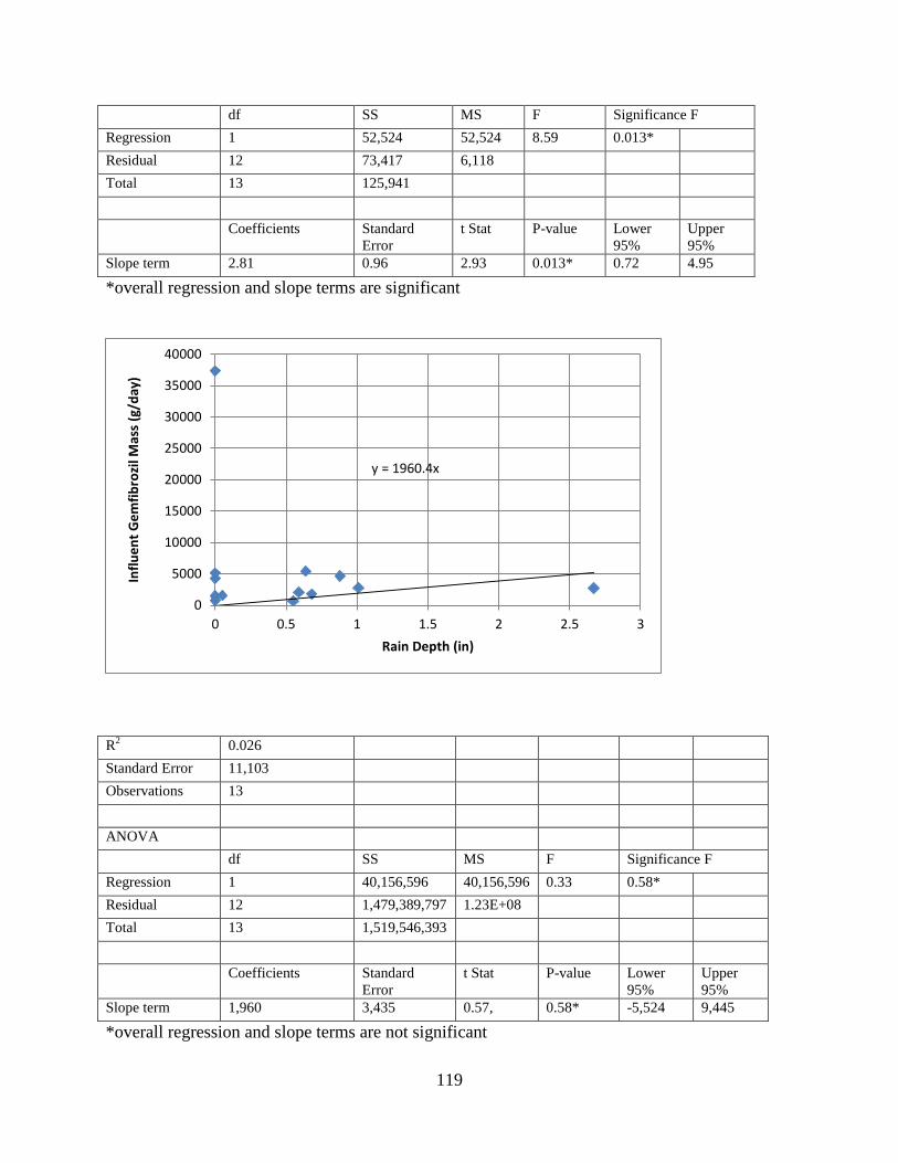
df SS MS F Significance F Regression 1 52,524 52,524 8.59 0.013* Residual 12 73,417 6,118 Total 13 125,941 Coefficients Standard
Error t Stat P-value Lower
95% Upper 95%
Slope term 2.81 0.96 2.93 0.013* 0.72 4.95
*overall regression and slope terms are significant
R2 0.026 Standard Error 11,103 Observations 13 ANOVA df SS MS F Significance F Regression 1 40,156,596 40,156,596 0.33 0.58* Residual 12 1,479,389,797 1.23E+08 Total 13 1,519,546,393 Coefficients Standard
Error t Stat P-value Lower
95% Upper 95%
Slope term 1,960 3,435 0.57, 0.58* -5,524 9,445
*overall regression and slope terms are not significant
y = 1960.4x
0
5000
10000
15000
20000
25000
30000
35000
40000
0 0.5 1 1.5 2 2.5 3
Influ
ent G
emfib
rozi
l Mas
s (g
/day
)
Rain Depth (in)
119

A.1.2. Summary Data for Ibuprofen Influe
nt (µg/L)
After Primary (µg/L)
After Secondary (µg/L)
Final Effluent (µg/L)
Daily Flow (MGD)
Mass Influent (g/day)
Daily Rain Depth at Tuscaloosa airport (in)
Overall % Reduction
1/16/2010 23 15 <dl <dl 18.2 1,582 0.55 100 3/2/2010 4.0 27 23 21 23.3 352 0.68 -425 4/24/2010 27 n/a* n/a n/a 16.5 1,684 1.01 n/a 6/25/2010 38 34 24 24 20.7 2,973 0.59 37 11/2/2010 30 26 22 22 2
0.5
2,325 0.88 27
3/9/2011 <dl <dl 27 <dl 42.2 <dl 2.67 Increase from <dl
5/11/2011 n/a 87 53 53 13.5 n/a 0.00 Increase from <dl
5/14/2011 188 48 48 <dl 30.7 21,817 0.00 100 9/20/2011 <dl <dl <dl <dl 26.5 <dl 0.64 n/a 3/20/2012 <dl <dl 39 39 17.1 0 0.00 Increase
from <dl 6/16/2012 <dl 25 <dl <dl 13.5 0 0.00 n/a 9/15/2012 <dl <dl <dl <dl 14.5 0 0.00 n/a 11/1/2012 51 62 <dl <dl 17.1 3,297 0.00 100 11/4/2012 <dl 29 26 30 15.4 0 0.05 Increase
from <dl Average dry (<0.1 inch of rain)
40 36 24 17 17.4 4,186 0.01 58 (calc. from averages)
Average wet 17 17 16 11 24.0 1,274 1.00 35 (calc. from averages)
* insufficient sample volume for analyses
120

Figure A.1.2.1. Probability plots for Ibuprofen
121

Figure A.1.2.2. Line graphs for Ibuprofen at four sampling locations Column Size Missing Mean Std Dev Std. Error C.I. of Mean influent 15 2 27.769 51.266 14.219 30.980 after primary 15 2 27.154 26.432 7.331 15.973 after secondary 15 2 20.154 19.034 5.279 11.502 effluent 15 2 14.538 18.219 5.053 11.010 flowMGD 10 0 22.900 8.462 2.676 6.053 rain depth 15 0 0.476 0.710 0.183 0.393 mass 9 1 3841.661 7344.657 2596.728 6140.287 Column Range Max Min Median 25% 75% influent 188.000 188.000 0.000 4.000 0.000 32.000
0.1
1
10
100
1000
Influent Primary Secondary Final
conc
(μg/
L)
Ibuprofen
01/16/10 (w)
03/02/10 (w)
04/24/10 (w)
06/25/10 (w)
11/02/10 (w)
03/09/11 (w)
05/11/11 (d)
05/14/11 (d)
09/20/11 (w)
03/20/12 (d)
06/16/12 (d)
09/15/12 (d)
11/01/12 (d)
11/04/12 (d)
11/08/12 (d)
11/12/12 (w)
MDL (upper)
MDL(lower)
122

after primary 87.000 87.000 0.000 26.000 0.000 37.500 after secondary 53.000 53.000 0.000 23.000 0.000 30.000 effluent 53.000 53.000 0.000 0.000 0.000 25.500 flowMGD 28.700 42.200 13.500 20.600 16.900 26.500 rain depth 2.670 2.670 0.000 0.0700 0.000 0.670 mass 21816.648 21816.648 0.000 1633.149 176.148 2649.024 Column Skewness Kurtosis K-S Dist. K-S Prob. SWilk W SWilk Prob influent 2.913 9.314 0.294 0.003 0.588 <0.001 after primary 0.982 0.787 0.167 0.385 0.888 0.090 after secondary 0.334 -1.070 0.240 0.040 0.866 0.046 effluent 0.900 -0.262 0.326 <0.001 0.794 0.006 flowMGD 1.438 2.213 0.203 0.279 0.881 0.134 rain depth 2.305 6.466 0.251 0.012 0.696 <0.001 mass 2.705 7.475 0.422 <0.001 0.556 <0.001
Figure A.1.2.3 Box and Whisker plots for Ibuprofen Normality Test (Shapiro-Wilk) Failed (P < 0.050) Kruskal-Wallis One Way Analysis of Variance on Ranks Group N Missing Median 25% 75% influent 15 2 4.000 0.000 34.000 after primary 15 2 26.000 0.000 41.000 after secondary 15 2 23.000 0.000 33.000 effluent 15 2 0.000 0.000 27.000 H = 1.955 with 3 degrees of freedom. (P = 0.582) The differences in the median values among the treatment groups are not great enough to exclude the possibility that the difference is due to random sampling variability; there is not a statistically significant difference (P = 0.582) Mann-Whitney Rank Sum Test
123

Normality Test (Shapiro-Wilk) Failed (P < 0.050) Group N Missing Median 25% 75% influent 15 2 4.000 0.000 34.000 after primary 15 2 26.000 0.000 41.000 Mann-Whitney U Statistic= 71.500 T = 162.500 n(small)= 13 n(big)= 13 (P = 0.509) The difference in the median values between the two groups is not great enough to exclude the possibility that the difference is due to random sampling variability; there is not a statistically significant difference (P = 0.509) Mann-Whitney Rank Sum Test Normality Test (Shapiro-Wilk) Failed (P < 0.050) Group N Missing Median 25% 75% after primary 15 2 26.000 0.000 41.000 after secondary 15 2 23.000 0.000 33.000 Mann-Whitney U Statistic= 70.500 T = 189.500 n(small)= 13 n(big)= 13 (P = 0.479) The difference in the median values between the two groups is not great enough to exclude the possibility that the difference is due to random sampling variability; there is not a statistically significant difference (P = 0.479) Mann-Whitney Rank Sum Test Normality Test (Shapiro-Wilk) Failed (P < 0.050) Group N Missing Median 25% 75% after secondary 15 2 23.000 0.000 33.000 effluent 15 2 0.000 0.000 27.000 Mann-Whitney U Statistic= 68.500 T = 191.500 n(small)= 13 n(big)= 13 (P = 0.402) The difference in the median values between the two groups is not great enough to exclude the possibility that the difference is due to random sampling variability; there is not a statistically significant difference (P = 0.402) Mann-Whitney Rank Sum Test Normality Test (Shapiro-Wilk) Failed (P < 0.050) Group N Missing Median 25% 75% influent 15 2 4.000 0.000 34.000 effluent 15 2 0.000 0.000 27.000
124

Mann-Whitney U Statistic= 75.500 T = 184.500 n(small)= 13 n(big)= 13 (P = 0.641) The difference in the median values between the two groups is not great enough to exclude the possibility that the difference is due to random sampling variability; there is not a statistically significant difference (P = 0.641)
R2 0.43 Standard Error 41.8 Observations 12 ANOVA df SS MS F Significance F Regression 1 13,228 13,228 7.57 0.020* Residual 10 17,475 1,748 Total 11 30,703 Coefficients Standard
Error t Stat P-value Lower
95% Upper 95%
Intercept -101 49.3 -2.06 0.067* -211 8.44 Slope term 6.74 2.45 2.75 0.020* 1.28 12.2
*overall regression, intercept (marginal), and slope terms are significant
y = 6.73x - 101 R² = 0.43; p = 0.02
1
10
100
1000
0 5 10 15 20 25 30 35Ibup
rofe
n in
fluen
t con
cent
ratio
ns (u
g/L)
Daily Treatment Plant Flow Rate (MGD)
125

R2 0.003 Standard Error 7,086 Observations 11 ANOVA df SS MS F Significance F Regression 1 1,560,312 1,560,312 0.031 0.86* Residual 10 502,145,820 50,214,582 Total 11 503,706,132 Coefficients Standard
Error t Stat P-value Lower
95% Upper 95%
Slope term 494 2,805 0.17 0.86* -5,756 6,745
*overall regression and slope terms are not significant A.1.3. Summary Data for Triclosan Influent
(µg/L) After Primary (µg/L)
After Secondary (µg/L)
Final Effluent (µg/L)
Daily Flow (MGD)
Mass Influent (g/day)
Daily Rain Depth at Tuscaloosa airport (in)
Overall % Reduction
1/16/2010 1.0 2.0 0.0 0.0 18.2 69 0.55 100 3/2/2010 4.0 2.0 0.0 0.0 23.3 352 0.68 100 4/24/2010 53 n/a n/a n/a 16.5 3,306 1.01 n/a 6/25/2010 8 5 <dl <dl 20.7 626 0.59 100 11/2/2010 <dl 7 7 8 20.5 n/a 0.88 n/a
y = 494x
0
5000
10000
15000
20000
25000
0 0.5 1 1.5 2 2.5
Influ
ent I
bupr
ofen
Mas
s (g
/day
)
Rain Depth (in.)
126
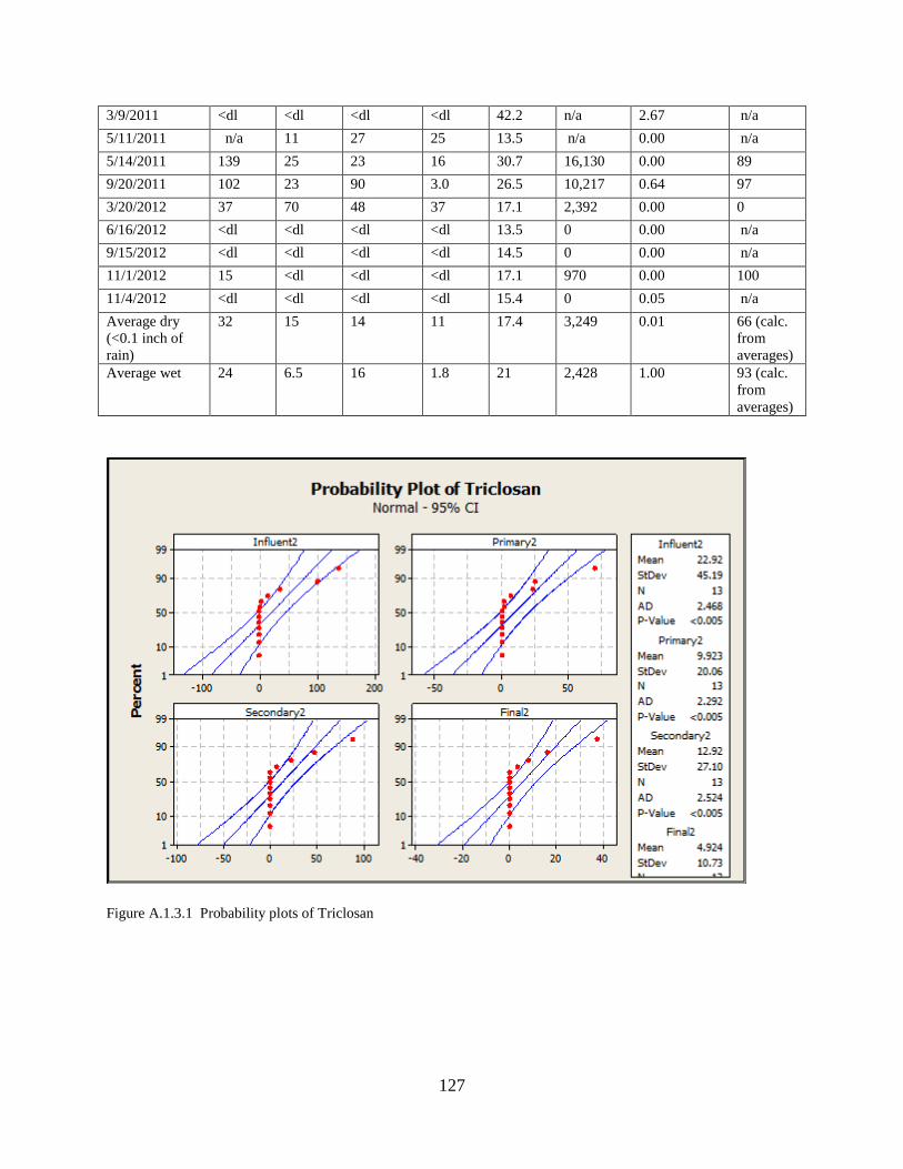
3/9/2011 <dl <dl <dl <dl 42.2 n/a 2.67 n/a 5/11/2011 n/a 11 27 25 13.5 n/a 0.00 n/a 5/14/2011 139 25 23 16 30.7 16,130 0.00 89 9/20/2011 102 23 90 3.0 26.5 10,217 0.64 97 3/20/2012 37 70 48 37 17.1 2,392 0.00 0 6/16/2012 <dl <dl <dl <dl 13.5 0 0.00 n/a 9/15/2012 <dl <dl <dl <dl 14.5 0 0.00 n/a 11/1/2012 15 <dl <dl <dl 17.1 970 0.00 100 11/4/2012 <dl <dl <dl <dl 15.4 0 0.05 n/a Average dry (<0.1 inch of rain)
32 15 14 11 17.4 3,249 0.01 66 (calc. from averages)
Average wet 24 6.5 16 1.8 21 2,428 1.00 93 (calc. from averages)
Figure A.1.3.1 Probability plots of Triclosan
127

Figure A.1.3.2 .Graph of Triclosan during Dry Weather
1
10
100
1000
Influent Primary Secondary Final
Conc
. μg/
L Triclosan
5/14/2011
3/20/2012
6/16/2012
9/15/2012
11/1/2012
Dry Weather
128

Figure A.1.3.3 Line plots of Triclosan at four sampling locations
Column Size Missing Mean Std Dev Std. Error C.I. of Mean influent 14 1 27.616 44.995 12.479 27.190 after primary 14 1 11.154 19.663 5.454 11.882 after secondary 14 1 15.000 27.058 7.505 16.351 final effluent 14 1 6.846 11.950 3.314 7.221 flow MGD 9 0 23.567 8.692 2.897 6.682 influent mass 9 1 3837.580 6073.540 2147.321 5077.606 rain depth 14 0 0.505 0.727 0.194 0.420 Column Range Max Min Median 25% 75% influent 139.000 139.000 0.000 4.000 0.000750 41.000 after primary 70.000 70.000 0.000 2.000 0.000 14.000 after secondary 90.000 90.000 0.000 0.001000 0.000 24.000 final effluent 37.000 37.000 0.000 0.001000 0.000 10.000 flow MGD 28.700 42.200 13.500 20.700 17.775 27.550 influent mass 16130.317 16130.394 0.0775 489.132 34.478 6761.475 rain depth 2.670 2.670 0.000 0.300 0.000 0.680
0.1
1
10
100
1000
Influent Primary Secondary Final
conc
(μg/
L)
Triclosan
01/16/10 (w)
03/02/10 (w)
04/24/10 (w)
06/25/10 (w)
11/02/10 (w)
03/09/11 (w)
05/11/10 (d)
05/14/11 (d)
09/20/11 (w)
03/20/12 (d)
06/16/12 (d)
09/15/12 (d)
11/01/12 (d)
11/04/12 (d)
11/08/12 (d)
11/12/12 (w)
MDL (upper)
MDL (lower)
129

Column Skewness Kurtosis K-S Dist. K-S Prob. SWilk W SWilk Prob influent 1.799 2.425 0.303 0.002 0.691 <0.001 after primary 2.582 7.271 0.285 0.005 0.633 <0.001 after secondary 2.150 4.628 0.326 <0.001 0.647 <0.001 final effluent 1.820 2.564 0.332 <0.001 0.662 <0.001 flow MGD 1.291 1.855 0.185 0.456 0.907 0.293 influent mass 1.594 1.495 0.327 0.012 0.714 0.003 rain depth 2.209 5.991 0.244 0.024 0.710 <0.001
Figure A.1.3.4 Box and Whisker plot of Triclosan Normality Test (Shapiro-Wilk) Failed (P < 0.050) Kruskal-Wallis One Way Analysis of Variance on Ranks Group N Missing Median 25% 75% influent 14 1 4.000 0.000500 45.000 after primary 14 1 2.000 0.000 17.000 after secondary 14 1 0.001000 0.000 25.000 final effluent 14 1 0.001000 0.000 12.000 H = 1.361 with 3 degrees of freedom. (P = 0.715) The differences in the median values among the treatment groups are not great enough to exclude the possibility that the difference is due to random sampling variability; there is not a statistically significant difference (P = 0.715) Mann-Whitney Rank Sum Test Normality Test (Shapiro-Wilk) Failed (P < 0.050)
130

Group N Missing Median 25% 75% influent 14 1 4.000 0.000500 45.000 after primary 14 1 2.000 0.000 17.000 Mann-Whitney U Statistic= 73.000 T = 187.000 n(small)= 13 n(big)= 13 (P = 0.569) The difference in the median values between the two groups is not great enough to exclude the possibility that the difference is due to random sampling variability; there is not a statistically significant difference (P = 0.569) Mann-Whitney Rank Sum Test Normality Test (Shapiro-Wilk) Failed (P < 0.050) Group N Missing Median 25% 75% after primary 14 1 2.000 0.000 17.000 after secondary 14 1 0.001000 0.000 25.000 Mann-Whitney U Statistic= 82.000 T = 178.000 n(small)= 13 n(big)= 13 (P = 0.917) The difference in the median values between the two groups is not great enough to exclude the possibility that the difference is due to random sampling variability; there is not a statistically significant difference (P = 0.917) Mann-Whitney Rank Sum Test Normality Test (Shapiro-Wilk) Failed (P < 0.050) Group N Missing Median 25% 75% after secondary 14 1 0.001000 0.000 25.000 final effluent 14 1 0.001000 0.000 12.000 Mann-Whitney U Statistic= 79.000 T = 181.000 n(small)= 13 n(big)= 13 (P = 0.792) The difference in the median values between the two groups is not great enough to exclude the possibility that the difference is due to random sampling variability; there is not a statistically significant difference (P = 0.792) Mann-Whitney Rank Sum Test Normality Test (Shapiro-Wilk) Failed (P < 0.050) Group N Missing Median 25% 75% influent 14 1 4.000 0.000500 45.000 final effluent 14 1 0.001000 0.000 12.000 Mann-Whitney U Statistic= 63.000 T = 197.000 n(small)= 13 n(big)= 13 (P = 0.274)
131

The difference in the median values between the two groups is not great enough to exclude the possibility that the difference is due to random sampling variability; there is not a statistically significant difference (P = 0.274)
R2 0.59 Standard Error 30.9 Observations 12 ANOVA df SS MS F Significance F
Regression 1 13,874 13,874 14.57 0.0035* Residual 10 9,595 959 Total 11 234,697 Coefficients Standard
Error t Stat P-value Lower
95% Upper 95%
Intercept -105 36.5 -2.87 0.017* -1867 -23.37 Slope term 6.90 1.81 3.80 0.0035* 2.86 10.9
*overall regression, intercept, and slope terms are significant
y = 6.9x - 105 R² = 0.59; p = 0.003
0.1
1
10
100
1000
0 5 10 15 20 25 30 35
Influ
ent T
riclo
san
(ug/
L)
Treatment Plant Daily Flow Rate (MGD)
132

R2 0.09 Standard Error 5,635 Observations 12 ANOVA df SS MS F Significance F Regression 1 33,367,332 33,367,332 1.05 0.33* Residual 11 349,323,899 31,756,718 Total 12 382,691,231 Coefficients Standard
Error t Stat P-value Lower
95% Upper 95%
Slope term 3,170 3,093 1.03 0.33* -3,637 9,978
*overall regression and slope terms are not significant
A.1.4. Summary Data for Carbamazepine
Influent (µg/L)
After Primary (µg/L)
After Secondary (µg/L)
Final Effluent (µg/L)
Daily Flow (MGD)
Mass Influent (g/day)
Daily Rain Depth at Tuscaloosa airport (in)
Overall % Reduction
1/16/2010 0.0 8.0 0.0 0.0 18.2 0 0.55 0 3/2/2010 0.0 5.0 5.0 7.0 23.3 0 0.68 0
0
2000
4000
6000
8000
10000
12000
14000
16000
18000
0.00 0.20 0.40 0.60 0.80 1.00 1.20
Influ
ent T
riclo
san
Mas
s (g/
day)
Daily Total Rainfall (inches)
133

4/24/2010 7.0 n/a n/a n/a 16.5 437 1.01 0 6/25/2010 0 10 2 2 20.7 0 0.59 0.0 11/2/2010 7 0 22 3 20.5 542 0.88 57.1 3/9/2011 0 0 0 0 42.2 0 2.67 0.0 5/11/2011 n/a 0.0 0.0 0.0 13.5 n/a 0.00 0.0 5/14/2011 0.0 0.0 0.0 0.0 30.7 0 0.00 0.0 9/20/2011 0.00 4.00 2.0 2.0 26.5 0 0.64 0.0 3/20/2012 0.0 0 0.0 0.0 17.1 0 0.00 0.0 6/16/2012 0.00 0.00 0.00 0.00 13.5 0 0.00 0.0 9/15/2012 0.00 0.00 9.0 3.0 14.5 0 0.00 0.0 11/1/2012 0.00 0.00 0.00 0.00 17.1 0 0.00 0.0 11/4/2012 0.00 4.0 2.0 2.0 15.4 0 0.05 0.0 11/8/2012 111.00 80.0 9.0 6.0 15.9 6,671 0.00 94.6 11/12/2012 5.00 8.0 4.0 4.0 16 302 0.44 20.0 Average dry (<0.1 inch of rain) 15.86 10.50 2.50 1.38 17.21 953.05 0.01
12 (calc. from averages)
Average wet
2.38 5.00 5.00 2.57 22.99 160.18 0.93
9.6 (calc. from averages)
100500-50-100
99
90
50
10
1100500-50
99
90
50
10
1
20100-10-20
99
90
50
10
11050-5
99
90
50
10
1
Influent_3
Perc
ent
Primary_3
Secondary_3 Final_3
Mean 9.286StDev 29.40N 14AD 4.112P-Value <0.005
Influent_3
Mean 7.929StDev 21.01N 14AD 3.465P-Value <0.005
Primary_3
Mean 3.929StDev 6.095N 14AD 1.561P-Value <0.005
Secondary_3
Mean 2.071StDev 2.336N 14
Final_3
Normal - 95% CICarbamazepine
134

Figure A.1.4.1. Probability Plot for Carbamazepine
Figure A.1.4.2 Line plot for Carbamazepine at four sampling locations Column Size Missing Mean Std Dev Std. Error C.I. of Mean Influent 16 1 8.667 28.432 7.341 15.745 After primary 16 1 7.933 20.250 5.229 11.214 After secondary 16 1 3.667 5.960 1.539 3.301 After final 16 1 1.933 2.314 0.597 1.281 Column Range Max Min Median 25% 75% Carbamazepine-Inf 111.000 111.000 0.000 0.000 0.000 3.750 Carbamazepine-Prim 80.000 80.000 0.000 0.000 0.000 7.250 Carbamazepine-Sec 22.000 22.000 0.000 2.000 0.000 4.750 Carbamazepine-Fin 7.000 7.000 0.000 2.000 0.000 3.000 Column Skewness Kurtosis K-S Dist. K-S Prob. SWilk W SWilk Prob Carbamazepine-Inf 3.817 14.683 0.457 <0.001 0.341 <0.001 Carbamazepine-Prim 3.674 13.879 0.393 <0.001 0.422 <0.001 Carbamazepine-Sec 2.378 6.322 0.277 0.003 0.673 <0.001 Carbamazepine-Fin 1.052 0.263 0.265 0.006 0.816 0.006 Column Sum Sum of Squares Carbamazepine-Inf 130.000 12444.000 Carbamazepine-Prim 119.000 6685.000 Carbamazepine-Sec 55.000 699.000 Carbamazepine-Fin 29.000 131.000
0.1
1.0
10.0
100.0
1000.0
Influent Primary Secondary Final
Conc
entr
atio
n (μ
g/L)
Carbamazepine
01/16/2010 (w)
3/2/2010 (w)
4/24/2010 (w)
6/25/2010 (w)
11/2/2010 (w)
9/20/2011 (w)
9/15/2012 (d)
11/4/2012 (d)
11/8/2012 (d)
11/12/2012 (w)
MDL (upper)
MDL (lower)
135

Figure A.1.4.3. Box and Whisker Plots for Carbamazepine One Way Analysis of Variance Data source: Data 1 in Notebook1 Normality Test (Shapiro-Wilk) Failed (P < 0.050) Test execution ended by user request, ANOVA on Ranks begun Kruskal-Wallis One Way Analysis of Variance on Ranks Data source: Data 1 in Notebook1 Group N Missing Median 25% 75% Col 1 16 1 0.000 0.000 5.000 Col 2 16 1 0.000 0.000 8.000 Col 3 16 1 2.000 0.000 5.000 Col 4 16 1 2.000 0.000 3.000 H = 1.574 with 3 degrees of freedom. (P = 0.665) The differences in the median values among the treatment groups are not great enough to exclude the possibility that the difference is due to random sampling variability; there is not a statistically significant difference (P = 0.665) Mann-Whitney Rank Sum Test Data source: Data 1 in Notebook1 Normality Test (Shapiro-Wilk) Failed (P < 0.050) Group N Missing Median 25% 75%
136
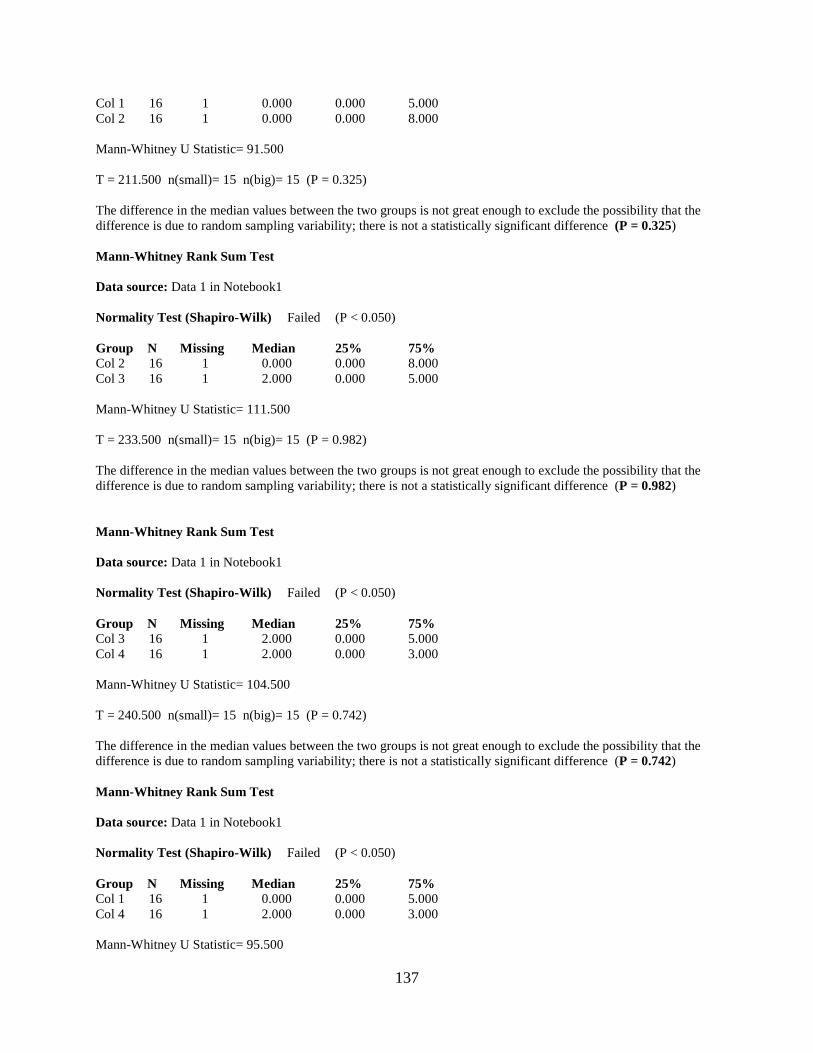
Col 1 16 1 0.000 0.000 5.000 Col 2 16 1 0.000 0.000 8.000 Mann-Whitney U Statistic= 91.500 T = 211.500 n(small)= 15 n(big)= 15 (P = 0.325) The difference in the median values between the two groups is not great enough to exclude the possibility that the difference is due to random sampling variability; there is not a statistically significant difference (P = 0.325) Mann-Whitney Rank Sum Test Data source: Data 1 in Notebook1 Normality Test (Shapiro-Wilk) Failed (P < 0.050) Group N Missing Median 25% 75% Col 2 16 1 0.000 0.000 8.000 Col 3 16 1 2.000 0.000 5.000 Mann-Whitney U Statistic= 111.500 T = 233.500 n(small)= 15 n(big)= 15 (P = 0.982) The difference in the median values between the two groups is not great enough to exclude the possibility that the difference is due to random sampling variability; there is not a statistically significant difference (P = 0.982) Mann-Whitney Rank Sum Test Data source: Data 1 in Notebook1 Normality Test (Shapiro-Wilk) Failed (P < 0.050) Group N Missing Median 25% 75% Col 3 16 1 2.000 0.000 5.000 Col 4 16 1 2.000 0.000 3.000 Mann-Whitney U Statistic= 104.500 T = 240.500 n(small)= 15 n(big)= 15 (P = 0.742) The difference in the median values between the two groups is not great enough to exclude the possibility that the difference is due to random sampling variability; there is not a statistically significant difference (P = 0.742) Mann-Whitney Rank Sum Test Data source: Data 1 in Notebook1 Normality Test (Shapiro-Wilk) Failed (P < 0.050) Group N Missing Median 25% 75% Col 1 16 1 0.000 0.000 5.000 Col 4 16 1 2.000 0.000 3.000 Mann-Whitney U Statistic= 95.500
137

T = 215.500 n(small)= 15 n(big)= 15 (P = 0.439) The difference in the median values between the two groups is not great enough to exclude the possibility that the difference is due to random sampling variability; there is not a statistically significant difference (P = 0.439)
A.1.5. Summary Data for Fluoxetine
Influent (µg/L)
After Primary (µg/L)
After Secondary (µg/L)
Final Effluent (µg/L)
Daily Flow (MGD)
Mass Influent (g/day)
Daily Rain Depth at Tuscaloosa airport (in)
Overall % Reduction
1/16/2010 30.0 18.0 0.0 0.0 18.2 2,064 0.55 100.0 3/2/2010 11.0 0.0 9.0 0.0 23.3 969 0.68 100.0 4/24/2010 10.0 n/a n/a n/a 16.5 624 1.01 0.0 6/25/2010 8 199 7 7 20.7 626 0.59 12.5 11/2/2010 18 24 0 0 20.5 1,395 0.88 100.0 3/9/2011 0 5 7 6 42.2 0 2.67 0.0 5/11/2011 n/a 120.0 13.0 0.0 13.5 0 0.00 0.0 5/14/2011 140.0 0.0 26.0 0.0 30.7 16,246 0.00 100.0 9/20/2011 8.00 6.00 0.0 0.0 26.5 801 0.64 100.0 3/20/2012 73.0 48 9.0 19.0 17.1 4,719 0.00 74.0 6/16/2012 17.00 24.0 5.0 12.0 13.5 868 0.00 29.4 9/15/2012 12.00 24.0 14.0 19.0 14.5 658 0.00 -58.3 11/1/2012 151.00 47.0 12.0 14.0 17.1 9,760 0.00 90.7 11/4/2012 1.00 13.0 5.0 5.0 15.4 58 0.05 -400.0 11/8/2012 38.00 18.0 9.0 8.0 15.9 2,284 0.00 78.9 11/12/2012 28.00 40.0 0.0 0.0 16 1,693 0.44 100.0 Average dry (<0.1 inch of rain) 61.71 36.75 11.63 9.63 17.21 4,941.81 0.01
-11 (calc. from averages)
Average wet
14.13 41.71 3.29 1.86 22.99 4,046.11 0.93
64 (calc. from averages)
138

2001000-100
99
90
50
10
12001000-100
99
90
50
10
1
3020100-10
99
90
50
10
1200-20
99
90
50
10
1
Influent_4
Perc
ent
Primary_4
Secondary_4 Final_4
Mean 36.33StDev 47.93N 15AD 1.908P-Value <0.005
Influent_4
Mean 39.07StDev 53.34N 15AD 1.837P-Value <0.005
Primary_4
Mean 7.733StDev 6.964N 15AD 0.534P-Value 0.143
Secondary_4
Mean 6StDev 7.051N 15
Final_4
Normal - 95% CIFluoxetine
Figure A.1.5.1. Probability plot for Fluoxetine
139

Figure A.1.5.2 Line graph of Fluoxetine at different sampling locations Column Size Missing Mean Std Dev Std. Error C.I. of Mean Fluoxetine-Inf 16 1 36.333 47.931 12.376 26.543 Fluoxetine-Prim 16 1 39.067 53.336 13.771 29.537 Fluoxetine-Sec 16 1 7.733 6.964 1.798 3.856 Fluoxetine-Final 16 1 6.000 7.051 1.821 3.905 Column Range Max Min Median 25% 75% Fluoxetine-Inf 151.000 151.000 0.000 17.000 8.500 36.000 Fluoxetine-Prim 199.000 199.000 0.000 24.000 7.750 45.250 Fluoxetine-Sec 26.000 26.000 0.000 7.000 1.250 11.250 Fluoxetine-Final 19.000 19.000 0.000 5.000 0.000 11.000
0.1
1.0
10.0
100.0
1000.0
Influent Primary Secondary Final
Conc
entr
atio
n μg
/L)
Fluoxetine
01/16/2010 (w)
3/2/2010 (w)
4/24/2010 (w)
6/25/2010 (w)
11/2/2010 (w)
3/9/2010 (w)
5/11/2011 (d)
5/14/2011 (d)
9/20/2011 (w)
3/20/2012 (d)
6/16/2012 (d)
9/15/2012 (d)
11/1/2012 (d)
11/4/2012 (d)
11/8/2012 (d)
11/12/2012 (w)
MDL (upper)
MDL (lower)
140

Column Skewness Kurtosis K-S Dist. K-S Prob. SWilk W SWilk Prob Fluoxetine-Inf 1.849 2.399 0.286 0.002 0.700 <0.001 Fluoxetine-Prim 2.379 5.809 0.300 <0.001 0.684 <0.001 Fluoxetine-Sec 1.142 2.231 0.161 0.348 0.884 0.054 Fluoxetine-Final 0.851 -0.586 0.269 0.005 0.812 0.005 Column Sum Sum of Squares Fluoxetine-Inf 545.000 51965.000 Fluoxetine-Prim 586.000 62720.000 Fluoxetine-Sec 116.000 1576.000 Fluoxetine-Final 90.000 1236.000
Figure A.1.5.3 Box and Whisker Plots for Fluoxetine One Way Analysis of Variance Data source: PHRM 2 in Notebook1 Normality Test (Shapiro-Wilk) Failed (P < 0.050) Test execution ended by user request, ANOVA on Ranks begun Kruskal-Wallis One Way Analysis of Variance on Ranks Data source: PHRM 2 in Notebook1 Group N Missing Median 25% 75% Col 6 16 1 17.000 8.000 38.000 Col 7 16 1 24.000 6.000 47.000 Col 8 16 1 7.000 0.000 12.000 Col 9 16 1 5.000 0.000 12.000
141

H = 15.108 with 3 degrees of freedom. (P = 0.002) The differences in the median values among the treatment groups are greater than would be expected by chance; there is a statistically significant difference (P = 0.002) To isolate the group or groups that differ from the others use a multiple comparison procedure. All Pairwise Multiple Comparison Procedures (Tukey Test): Comparison Diff of Ranks q P<0.05 Col 7 vs Col 9 292.500 4.324 Yes Col 7 vs Col 8 237.500 3.511 No Col 7 vs Col 6 14.000 0.207 Do Not Test Col 6 vs Col 9 278.500 4.117 Yes Col 6 vs Col 8 223.500 3.304 Do Not Test Col 8 vs Col 9 55.000 0.813 No Mann-Whitney Rank Sum Test Data source: PHRM 2 in Notebook1 Normality Test (Shapiro-Wilk) Failed (P < 0.050) Group N Missing Median 25% 75% Col 6 16 1 17.000 8.000 38.000 Col 7 16 1 24.000 6.000 47.000 Mann-Whitney U Statistic= 105.000 T = 225.000 n(small)= 15 n(big)= 15 (P = 0.771) The difference in the median values between the two groups is not great enough to exclude the possibility that the difference is due to random sampling variability; there is not a statistically significant difference (P = 0.771) Mann-Whitney Rank Sum Test Data source: PHRM 2 in Notebook1 Normality Test (Shapiro-Wilk) Failed (P < 0.050) Group N Missing Median 25% 75% Col 7 16 1 24.000 6.000 47.000 Col 8 16 1 7.000 0.000 12.000 Mann-Whitney U Statistic= 52.500 T = 292.500 n(small)= 15 n(big)= 15 (P = 0.013) The difference in the median values between the two groups is greater than would be expected by chance; there is a statistically significant difference (P = 0.013) Mann-Whitney Rank Sum Test
142

Data source: PHRM 2 in Notebook1 Normality Test (Shapiro-Wilk) Failed (P < 0.050) Group N Missing Median 25% 75% Col 8 16 1 7.000 0.000 12.000 Col 9 16 1 5.000 0.000 12.000 Mann-Whitney U Statistic= 93.000 T = 252.000 n(small)= 15 n(big)= 15 (P = 0.418) The difference in the median values between the two groups is not great enough to exclude the possibility that the difference is due to random sampling variability; there is not a statistically significant difference (P = 0.418) Mann-Whitney Rank Sum Test Data source: PHRM 2 in Notebook1 Normality Test (Shapiro-Wilk) Failed (P < 0.050) Group N Missing Median 25% 75% Col 6 16 1 17.000 8.000 38.000 Col 9 16 1 5.000 0.000 12.000 Mann-Whitney U Statistic= 44.000 T = 301.000 n(small)= 15 n(big)= 15 (P = 0.004) The difference in the median values between the two groups is greater than would be expected by chance; there is a statistically significant difference (P = 0.004)
A.1.6. Summary Data for Sulfamethoxazole
Influent (µg/L)
After Primary (µg/L)
After Secondary (µg/L)
Final Effluent (µg/L)
Daily Flow (MGD)
Mass Influent (g/day)
Daily Rain Depth at Tuscaloosa airport (in)
Overall % Reduction
1/16/2010 0.0 0.0 14.0 12.0 18.2 0 0.55 0.0 3/2/2010 26.0 70.0 22.0 24.0 23.3 2,290 0.68 7.7 4/24/2010 13.0 n/a n/a n/a 16.5 811 1.01 0.0 6/25/2010 10 16 9 10 20.7 782 0.59 0.0 11/2/2010 23 21 10 10 20.5 1,782 0.88 56.5 3/9/2011 11 12 12 10 42.2 1,755 2.67 9.1 5/11/2011 n/a 0.0 57.0 0.0 13.5 0.00 0.0 5/14/2011 247.0 46.0 0.0 42.0 30.7 28,663 0.00 83.0 9/20/2011 0.00 10.00 24.0 13.0 26.5 0 0.64 0.0 3/20/2012 0.0 28 50.0 31.0 17.1 0 0.00 0.0
143

6/16/2012 0.00 14.0 9.0 19.0 13.5 0 0.00 0.0 9/15/2012 10.00 20.0 34.0 25.0 14.5 548 0.00 -150.0 11/1/2012 0.00 160.0 22.0 0.0 17.1 0 0.00 0.0 11/4/2012 0.00 10.0 24.0 13.0 15.4 0 0.05 0.0 11/8/2012 224.00 63.0 53.0 65.0 15.9 13,463 0.00 71.0 11/12/2012 0.00 0.0 12.0 13.0 16 0 0.44 0.0 Average dry (<0.1 inch of rain) 68.71 42.63 31.13 24.38 17.21 6,096.33 0.01
0.50 (from average)
Average wet
10.38 18.43 14.71 13.14 22.99 927.52 0.93
9.16 (from average)
3001500-150-300
99
90
50
10
12001000-100
99
90
50
10
1
500-50
99
90
50
10
1500-50
99
90
50
10
1
Influent_5
Perc
ent
Primary_5
Secondary_5 Final_5
Mean 37.6StDev 80.92N 15AD 3.502P-Value <0.005
Influent_5
Mean 31.33StDev 41.64N 15AD 1.520P-Value <0.005
Primary_5
Mean 23.47StDev 17.57N 15AD 0.781P-Value 0.033
Secondary_5
Mean 19.13StDev 16.84N 15
Final_5
Normal - 95% CISulfamethoxazole
Figure A.1.6.1 Probability Plot for Sulfamethoxazole
144

Figure A.1.6.2 Line graph for Sulfamethoxazole at different sampling locations Column Size Missing Mean Std Dev Std. Error C.I. of Mean SMX-I 16 1 37.600 80.920 20.894 44.812 SMX-P 16 1 31.333 41.644 10.752 23.062 SMX-S 16 1 23.467 17.566 4.535 9.728 SMX-F 16 1 19.133 16.843 4.349 9.327 Column Range Max Min Median 25% 75% SMX-I 247.000 247.000 0.000 10.000 0.000 20.500 SMX-P 160.000 160.000 0.000 16.000 10.000 41.500 SMX-S 57.000 57.000 0.000 22.000 10.500 31.500 SMX-F 65.000 65.000 0.000 13.000 10.000 24.750 Column Skewness Kurtosis K-S Dist. K-S Prob. SWilk W SWilk Prob SMX-I 2.365 4.293 0.424 <0.001 0.506 <0.001 SMX-P 2.388 6.497 0.265 0.006 0.712 <0.001 SMX-S 0.882 -0.307 0.221 0.047 0.880 0.048 SMX-F 1.606 3.080 0.242 0.018 0.845 0.015 Column Sum Sum of Squares SMX-I 564.000 112880.000 SMX-P 470.000 39006.000 SMX-S 352.000 12580.000
0.1
1.0
10.0
100.0
1000.0
Influent Primary Secondary Final
Conc
entr
atio
n (μ
g/L)
Sulfamethoxazole
01/16/2010 (w)
3/2/2010 (w)
4/24/2010 (w)
6/25/2010 (w)
11/2/2010 (w)
3/9/2010 (w)
5/11/2011 (d)
5/14/2011 (d)
9/20/2011 (w)
3/20/2012 (d)
6/16/2012 (d)
9/15/2012 (d)
11/1/2012 (d)
11/4/2012 (d)
11/8/2012 (d)
11/12/2012 (w)
145

SMX-F 287.000 9463.000
Figure A.1.6.3. Box and Whisker Plots for Sulfamethoxazole One Way Analysis of Variance Data source: PHRM 2 in Notebook1 Normality Test (Shapiro-Wilk) Failed (P < 0.050) Test execution ended by user request, ANOVA on Ranks begun Kruskal-Wallis One Way Analysis of Variance on Ranks Data source: PHRM 2 in Notebook1 Group N Missing Median 25% 75% Col 11 16 1 10.000 0.000 23.000 Col 12 16 1 16.000 10.000 46.000 Col 13 16 1 22.000 10.000 34.000 Col 14 16 1 13.000 10.000 25.000 H = 3.754 with 3 degrees of freedom. (P = 0.289) The differences in the median values among the treatment groups are not great enough to exclude the possibility that the difference is due to random sampling variability; there is not a statistically significant difference (P = 0.289) Mann-Whitney Rank Sum Test Data source: PHRM 2 in Notebook1 Normality Test (Shapiro-Wilk) Failed (P < 0.050) Group N Missing Median 25% 75%
146

Col 11 16 1 10.000 0.000 23.000 Col 12 16 1 16.000 10.000 46.000 Mann-Whitney U Statistic= 79.500 T = 199.500 n(small)= 15 n(big)= 15 (P = 0.169) The difference in the median values between the two groups is not great enough to exclude the possibility that the difference is due to random sampling variability; there is not a statistically significant difference (P = 0.169) Mann-Whitney Rank Sum Test Data source: PHRM 2 in Notebook1 Normality Test (Shapiro-Wilk) Failed (P < 0.050) Group N Missing Median 25% 75% Col 12 16 1 16.000 10.000 46.000 Col 13 16 1 22.000 10.000 34.000 Mann-Whitney U Statistic= 109.000 T = 229.000 n(small)= 15 n(big)= 15 (P = 0.901) The difference in the median values between the two groups is not great enough to exclude the possibility that the difference is due to random sampling variability; there is not a statistically significant difference (P = 0.901) Mann-Whitney Rank Sum Test Data source: PHRM 2 in Notebook1 Normality Test (Shapiro-Wilk) Failed (P < 0.050) Group N Missing Median 25% 75% Col 13 16 1 22.000 10.000 34.000 Col 14 16 1 13.000 10.000 25.000 Mann-Whitney U Statistic= 100.500 T = 244.500 n(small)= 15 n(big)= 15 (P = 0.632) The difference in the median values between the two groups is not great enough to exclude the possibility that the difference is due to random sampling variability; there is not a statistically significant difference (P = 0.632) Mann-Whitney Rank Sum Test Data source: PHRM 2 in Notebook1 Normality Test (Shapiro-Wilk) Failed (P < 0.050) Group N Missing Median 25% 75% Col 11 16 1 10.000 0.000 23.000 Col 14 16 1 13.000 10.000 25.000 Mann-Whitney U Statistic= 78.500
147

T = 198.500 n(small)= 15 n(big)= 15 (P = 0.158) The difference in the median values between the two groups is not great enough to exclude the possibility that the difference is due to random sampling variability; there is not a statistically significant difference (P = 0.158)
A.1.7. Summary Data for Trimethoprim
Influent (µg/L)
After Primary (µg/L)
After Secondary (µg/L)
Final Effluent (µg/L)
Daily Flow (MGD)
Mass Influent (g/day)
Daily Rain Depth at Tuscaloosa airport (in)
Overall % Reduction
1/16/2010 0.0 0.0 16.0 14.0 18.2 0 0.55 0.0 3/2/2010 25.0 22.0 0.0 0.0 23.3 2,202 0.68 100.0 4/24/2010 0.0 n/a n/a n/a 16.5 0 1.01 0.0 6/25/2010 0 0 0 0 20.7 0 0.59 0.0 11/2/2010 0 0 0 0 20.5 0 0.88 0.0 3/9/2011 0 0 0 0 42.2 0 2.67 0.0 5/11/2011 n/a 0.0 38.0 34.0 13.5 0 0.00 0.0 5/14/2011 0.0 37.0 0.0 28.0 30.7 0 0.00 0.0 9/20/2011 0.00 0.00 11.0 0.0 26.5 0 0.64 0.0 3/20/2012 43.0 47 23.0 29.0 17.1 2,779 0.00 32.6 6/16/2012 12.00 0.0 0.0 0.0 13.5 612 0.00 100.0 9/15/2012 22.00 89.0 63.0 63.0 14.5 1,206 0.00 -186.4 11/1/2012 37.00 43.0 0.0 0.0 17.1 2,392 0.00 100.0 11/4/2012 0.00 0.0 14.0 0.0 15.4 0 0.05 0.0 11/8/2012 0.00 10.0 31.0 14.0 15.9 0 0.00 0.0 11/12/2012 0.00 0.00 0.00 0.00 16 0 0.44 0.0 Average dry (<0.1 inch of rain)
16.29 28.25 21.13 21.00 17.21 998.46 0.01
5.77 (calc from avg)
Average wet
3.13 3.14 3.86 2.00 22.99 275.23 0.93
11.11 (calc from avg)
148
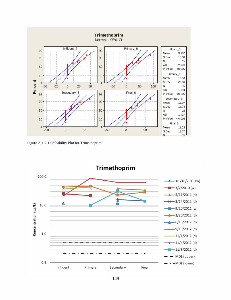
50250-25-50
99
90
50
10
1100500-50
99
90
50
10
1
500-50
99
90
50
10
1500-50
99
90
50
10
1
Influent_6
Perc
ent
Primary_6
Secondary_6 Final_6
Mean 9.267StDev 15.08N 15AD 2.276P-Value <0.005
Influent_6
Mean 16.53StDev 26.50N 15AD 1.894P-Value <0.005
Primary_6
Mean 13.07StDev 18.74N 15AD 1.427P-Value <0.005
Secondary_6
Mean 12.13StDev 18.77N 15
Final_6
Normal - 95% CITrimethoprim
Figure A.1.7.1 Probability Plot for Trimethoprim
0.1
1.0
10.0
100.0
Influent Primary Secondary Final
Conc
entr
atio
n (μ
g/L)
Trimethoprim
01/16/2010 (w)
3/2/2010 (w)
5/11/2011 (d)
5/14/2011 (d)
9/20/2011 (w)
3/20/2012 (d)
6/16/2012 (d)
9/15/2012 (d)
11/1/2012 (d)
11/4/2012 (d)
11/8/2012 (d)
MDL (upper)
MDL (lower)
149

Figure A.1.7.2 Line graph for Trimethoprim at different sampling locations Column Size Missing Mean Std Dev Std. Error C.I. of Mean TRM-I 16 1 9.267 15.078 3.893 8.350 TRM-P 16 1 16.533 26.500 6.842 14.675 TRM-S 16 1 13.067 18.737 4.838 10.376 TRM-F 16 1 12.133 18.773 4.847 10.396 Column Range Max Min Median 25% 75% TRM-I 43.000 43.000 0.000 0.000 0.000 19.500 TRM-P 89.000 89.000 0.000 0.000 0.000 33.250 TRM-S 63.000 63.000 0.000 0.000 0.000 21.250 TRM-F 63.000 63.000 0.000 0.000 0.000 24.500 Column Skewness Kurtosis K-S Dist. K-S Prob. SWilk W SWilk Prob TRM-I 1.388 0.584 0.397 <0.001 0.676 <0.001 TRM-P 1.750 2.866 0.334 <0.001 0.699 <0.001 TRM-S 1.615 2.427 0.291 0.001 0.756 0.001 TRM-F 1.679 2.657 0.341 <0.001 0.713 <0.001 Column Sum Sum of Squares TRM-I 139.000 4471.000 TRM-P 248.000 13932.000 TRM-S 196.000 7476.000 TRM-F 182.000 7142.000
Figure A.1.7.2 Box and Whisker Plots for Trimethoprim One Way Analysis of Variance Data source: PHRM 2 in Notebook1 Normality Test (Shapiro-Wilk) Failed (P < 0.050)
150

Test execution ended by user request, ANOVA on Ranks begun Kruskal-Wallis One Way Analysis of Variance on Ranks Data source: PHRM 2 in Notebook1 Group N Missing Median 25% 75% Col 16 16 1 0.000 0.000 22.000 Col 17 16 1 0.000 0.000 37.000 Col 18 16 1 0.000 0.000 23.000 Col 19 16 1 0.000 0.000 28.000 H = 0.514 with 3 degrees of freedom. (P = 0.916) The differences in the median values among the treatment groups are not great enough to exclude the possibility that the difference is due to random sampling variability; there is not a statistically significant difference (P = 0.916) Mann-Whitney Rank Sum Test Data source: PHRM 2 in Notebook1 Normality Test (Shapiro-Wilk) Failed (P < 0.050) Group N Missing Median 25% 75% Col 16 16 1 0.000 0.000 22.000 Col 17 16 1 0.000 0.000 37.000 Mann-Whitney U Statistic= 100.500 T = 220.500 n(small)= 15 n(big)= 15 (P = 0.581) The difference in the median values between the two groups is not great enough to exclude the possibility that the difference is due to random sampling variability; there is not a statistically significant difference (P = 0.581) Mann-Whitney Rank Sum Test Data source: PHRM 2 in Notebook1 Normality Test (Shapiro-Wilk) Failed (P < 0.050) Group N Missing Median 25% 75% Col 17 16 1 0.000 0.000 37.000 Col 18 16 1 0.000 0.000 23.000 Mann-Whitney U Statistic= 111.000 T = 231.000 n(small)= 15 n(big)= 15 (P = 0.963) The difference in the median values between the two groups is not great enough to exclude the possibility that the difference is due to random sampling variability; there is not a statistically significant difference (P = 0.963) Mann-Whitney Rank Sum Test
151

Data source: PHRM 2 in Notebook1 Normality Test (Shapiro-Wilk) Failed (P < 0.050) Group N Missing Median 25% 75% Col 18 16 1 0.000 0.000 23.000 Col 19 16 1 0.000 0.000 28.000 Mann-Whitney U Statistic= 106.500 T = 238.500 n(small)= 15 n(big)= 15 (P = 0.801) The difference in the median values between the two groups is not great enough to exclude the possibility that the difference is due to random sampling variability; there is not a statistically significant difference (P = 0.801) Mann-Whitney Rank Sum Test Data source: PHRM 2 in Notebook1 Normality Test (Shapiro-Wilk) Failed (P < 0.050) Group N Missing Median 25% 75% Col 16 16 1 0.000 0.000 22.000 Col 19 16 1 0.000 0.000 28.000 Mann-Whitney U Statistic= 104.000 T = 224.000 n(small)= 15 n(big)= 15 (P = 0.701) The difference in the median values between the two groups is not great enough to exclude the possibility that the difference is due to random sampling variability; there is not a statistically significant difference (P = 0.701)
A.2. Polycyclic Aromatic Hydrocarbons (PAHs)
A.2.1. Summary Data for Naphthalene
Influent (µg/L)
After Primary (µg/L)
After Secondary (µg/L)
Final Effluent (µg/L)
Daily Flow (MGD)
Mass Influent (g/day)
Daily Rain Depth at Tuscaloosa airport (in)
Overall % Reduction
1/16/2010 57.0 350.0 190 160 18.2 3,921 0.55 -180.7 3/2/2010 1.7 10.5 5.6 4.7 23.3 151 0.68 -175.1 4/24/2010 20.7 16.7 0.4 4.7 16.5 1,289 1.01 77.2 6/25/2010 0.33 0.25 0.27 0.33 20.7 26 0.59 0.4 10/17/2010 14 16.3 0.072 2.7 15.3 805 0.00 80.8 10.24/2010 20.7 16.7 0.4 4.7 15.7 1,227 0.10 77.2
152

11/2/2010 2.5 13 0.73 0.049 20.5 196 0.88 98.1 3/9/2011 7.7 18 BQ n/a 42.2 1,231 2.67 0.0 5/11/2011 30.4 50.9 8.0 0.0 13.5 1,552 0.00 100.0 5/14/2011 17.0 14.0 11.3 1.5 30.7 1,971 0.00 91.2 9/20/2011 0.86 0.84 2.5 7.3 26.5 86 0.64 -745.0 10/10/2011 0.18 4.33 10.8 4.6 16.9 11 0.00 -2477.4 3/20/2012 7.1 17 5.4 2.7 17.1 456 0.00 62.0 6/16/2012 0.62 6.7 2.4 BDL 13.5 32 0.00 100.0 9/15/2012 0.0 0.0 0.0 0.0 14.5 0 0.00 0.0 11/1/2012 1.1 1.7 0.0 0.0 17.1 72 0.00 100.0 11/4/2012 0.14 0.58 0.0 0.0 15.4 8 0.05 100.0 11/8/2012 0.14 0 0.0 0.0 15.9 8 0.00 100.0 11/12/2012 26 0.054 0.0 0.0 16.0 1,571 0.44 100.0 Average dry (<0.1 inch of rain)
7.058 11.143 3.811 1.273 16.990 491.692 0.005
-174 (calc from avg)
Average wet
15.27 47.24 24.99 22.72 22.18 1,077.57 0.84
-83.10 (calc from avg)
50250-25-50
99
90
50
10
14002000-200
99
90
50
10
1
2001000-100
99
90
50
10
12001000-100
99
90
50
10
1
Influent_7
Perc
ent
Primary_7
Secondary_7 Final_7
Mean 10.95StDev 14.96N 19AD 1.586P-Value <0.005
Influent_7
Mean 28.24StDev 78.84N 19AD 5.019P-Value <0.005
Primary_7
Mean 13.22StDev 44.28N 18AD 5.350P-Value <0.005
Secondary_7
Mean 11.36StDev 38.37N 17
Final_7
Normal - 95% CINaphthalene
Figure A.2.1.1. Probability plots for Naphthalene
153

Figure A.2.1.2.Graph of Naphthalene during Wet Weather
0.1
1
10
100
1000
Influent Primary Secondary Final
conc
μg/
L Naphthalene
01/16/2010
3/2/2010
4/24/2010
154

Figure A.2.1.3. Graph of Naphthalene during Dry Weather
0.01
0.1
1
10
100
Influent Primary Secondary Final
Conc
μg/
L
Naphthlene
10/24/2010
5/11/2011
5/14/2011
3/20/2012
155

Figure A.2.1.4. Line graph for Naphthalene (total) at four sampling locations Descriptive Statistics: Data source: PAH in PAH 2010-2012 Column Size Missing Mean Std Dev Std. Error C.I. of Mean Naphthalene-I 19 0 10.950 14.962 3.432 7.211 Naphthalene-P 19 0 28.241 78.841 18.087 38.000 Naphthalene-S 19 1 13.224 44.283 10.437 22.021 Naphthalene-F 19 2 11.365 38.374 9.307 19.730 Column Range Max Min Median 25% 75% Naphthalene-I 56.996 56.996 0.000 2.528 0.402 19.751 Naphthalene-P 350.000 350.000 0.000 10.458 0.644 16.666 Naphthalene-S 190.000 190.000 0.000 0.579 0.000 5.567 Naphthalene-F 160.000 160.000 0.000 1.490 0.000 4.704
0.0
0.1
1.0
10.0
100.0
1000.0
Influent Primary Secondary Final
Conc
entr
atio
n (μ
g/L)
Naphathlene
01/16/2010 (w)
3/2/2010 (w)
4/24/2010 (w)
6/25/2010 (w)
10/17/2010 (d)
10/24/2010 (w)
11/2/2010 (w)
3/9/2010 (w)
5/11/2011 (d)
5/14/2011 (d)
9/20/2011 (w)
10/10/2011 (d)
3/20/2012 (d)
6/16/2012 (d)
11/1/2012 (d)
11/4/2012 (d)
11/8/2012 (d)
11/12/2012 (w)
156

Column Skewness Kurtosis K-S Dist. K-S Prob. SWilk W SWilk Prob Naphthalene-I 1.847 3.894 0.240 0.005 0.757 <0.001 Naphthalene-P 4.197 17.967 0.448 <0.001 0.355 <0.001 Naphthalene-S 4.190 17.682 0.462 <0.001 0.316 <0.001 Naphthalene-F 4.097 16.848 0.484 <0.001 0.310 <0.001 Column Sum Sum of Squares Naphthalene-I 208.053 6307.469 Naphthalene-P 536.588 127040.994 Naphthalene-S 238.032 36483.767 Naphthalene-F 193.205 25756.844
Figure A.2.1.5. Box and Whisker plot for Naphthalene One Way Analysis of Variance Data source: PAH in Notebook1 Normality Test (Shapiro-Wilk) Failed (P < 0.050) Test execution ended by user request, ANOVA on Ranks begun Kruskal-Wallis One Way Analysis of Variance on Ranks Data source: PAH in Notebook1 Group N Missing Median 25% 75% Col 1 19 0 2.528 0.329 20.673 Col 2 19 0 10.458 0.580 16.666 Col 3 19 1 0.579 0.000 6.187
157

Col 4 19 2 1.490 0.000 4.704 H = 7.681 with 3 degrees of freedom. (P = 0.053) The differences in the median values among the treatment groups are not great enough to exclude the possibility that the difference is due to random sampling variability; there is not a statistically significant difference (P = 0.053) Mann-Whitney Rank Sum Test Data source: PAH in Notebook1 Normality Test (Shapiro-Wilk) Failed (P < 0.050) Group N Missing Median 25% 75% Col 1 19 0 2.528 0.329 20.673 Col 2 19 0 10.458 0.580 16.666 Mann-Whitney U Statistic= 176.000 T = 366.000 n(small)= 19 n(big)= 19 (P = 0.907) The difference in the median values between the two groups is not great enough to exclude the possibility that the difference is due to random sampling variability; there is not a statistically significant difference (P = 0.907) Mann-Whitney Rank Sum Test Data source: PAH in Notebook1 Normality Test (Shapiro-Wilk) Failed (P < 0.050) Group N Missing Median 25% 75% Col 2 19 0 10.458 0.580 16.666 Col 3 19 1 0.579 0.000 6.187 Mann-Whitney U Statistic= 102.000 T = 273.000 n(small)= 18 n(big)= 19 (P = 0.037) The difference in the median values between the two groups is greater than would be expected by chance; there is a statistically significant difference (P = 0.037) Mann-Whitney Rank Sum Test Data source: PAH in Notebook1 Normality Test (Shapiro-Wilk) Failed (P < 0.050) Group N Missing Median 25% 75% Col 3 19 1 0.579 0.000 6.187 Col 4 19 2 1.490 0.000 4.704 Mann-Whitney U Statistic= 142.500 T = 295.500 n(small)= 17 n(big)= 18 (P = 0.738)
158

The difference in the median values between the two groups is not great enough to exclude the possibility that the difference is due to random sampling variability; there is not a statistically significant difference (P = 0.738) Mann-Whitney Rank Sum Test Sunday, January 13, 2013, 2:09:25 PM Data source: PAH in Notebook1 Normality Test (Shapiro-Wilk) Failed (P < 0.050) Group N Missing Median 25% 75% Col 1 19 0 2.528 0.329 20.673 Col 4 19 2 1.490 0.000 4.704 Mann-Whitney U Statistic= 106.500 T = 259.500 n(small)= 17 n(big)= 19 (P = 0.083) The difference in the median values between the two groups is not great enough to exclude the possibility that the difference is due to random sampling variability; there is not a statistically significant difference (P = 0.083)
A.2.2. Summary Data for Acenaphthene
Influent (µg/L)
After Primary (µg/L)
After Secondary (µg/L)
Final Effluent (µg/L)
Daily Flow (MGD)
Mass Influent (g/day)
Daily Rain Depth at Tuscaloosa airport (in)
Overall % Reduction
1/16/2010 57.0 21.4 0.0 0.0 18.2 3921.1 0.55 100.0 3/2/2010 1.7 0.6 0.0 0.0 23.3 150.6 0.68 100.0 4/24/2010 20.7 3.1 2.5 4.2 16.5 1289.3 1.01 79.8 6/25/2010 0.33 0.099 0.036 0.022 20.7 25.8 0.59 93.3 10/17/2010 14 3.4 BDL 0.051 15.3 805.0 0.00 99.6 10.24/2010 20.7 4.8 0.2 0.2 15.7 1226.8 0.10 99.2 11/2/2010 2.5 0.97 BDL BQ 20.5 195.9 0.88 100.0 3/9/2011 7.7 2.3 BQ n/a 42.2 1231.1 2.67 100.0 5/11/2011 30.4 0.9 0.0 0.0 13.5 1552.4 0.00 100.0 5/14/2011 17.0 0.7 BQ BQ 30.7 1971.3 0.00 100.0 9/20/2011 0.86 0.29 0.00 0.085 26.5 86.0 0.64 90.0 10/10/2011 0.18 0.25 0.63 0.018 16.9 11.4 0.00 90.1 3/20/2012 7.1 2.4 0.16 0.088 17.1 456.2 0.00 98.8 6/16/2012 0.62 0.35 0.01 BDL 13.5 31.6 0.00 100.0 9/15/2012 0.00 0.00 0.00 0.0 14.5 0.0 0.00 0.0 11/1/2012 0.14 0.14 0.00 0.0 17.1 9.1 0.00 100.0
159

11/4/2012 0.00 0.00 0.00 0.00 15.4 0.0 0.05 0.0 11/8/2012 BQ 0.00 0.00 0.00 15.9 0.0 0.00 0.0 11/12/2012 BQ BQ 0.01 0.00 16.0 0.0 0.44 0.0 Average dry (<0.1 inch of rain) 7.70 0.82 0.10 0.02 16.99 483.71 0.01
68 (calc from avg)
Average wet
16.87 5.07 0.39 0.64 19.56 957.09 0.57
80. (calc from avg)
50250-25-50
99
90
50
10
120100-10
99
90
50
10
1
210-1-2
99
90
50
10
1420-2-4
99
90
50
10
1
Influent_8
Perc
ent
Primary_8
Secondary_8 Final_8
Mean 10.64StDev 15.22N 17AD 1.551P-Value <0.005
Influent_8
Mean 2.324StDev 4.977N 18AD 3.415P-Value <0.005
Primary_8
Mean 0.2343StDev 0.6511N 15AD 3.773P-Value <0.005
Secondary_8
Mean 0.3081StDev 1.073N 15
Final_8
Normal - 95% CIAcenaphthene
Figure A.2.2.1. Probability Plot for Acenaphthene
160

Figure A.2.2.2 Line graph for Acenaphthene at four different sampling locations Column .Size Missing Mean Std Dev Std. Error C.I. of Mean Acenaphthene-I 19 2 10.636 15.223 3.692 7.827 Acenaphthene-P 19 1 2.324 4.977 1.173 2.475 Acenaphthene-S 19 4 0.234 0.651 0.168 0.361 Acenaphthene-F 19 4 0.308 1.073 0.277 0.594 Column Range Max Min Median 25% 75% Acenaphthene-I 56.996 56.996 0.000 2.528 0.292 17.909 Acenaphthene-P 21.447 21.447 0.000 0.672 0.141 2.428 Acenaphthene-S 2.513 2.513 0.000 0.000 0.000 0.126 Acenaphthene-F 4.182 4.182 0.000 0.000 0.000 0.0770 Column Skewness Kurtosis K-S Dist. K-S Prob. SWilk W SWilk Prob Acenaphthene-I 2.021 4.628 0.242 0.009 0.737 <0.001 Acenaphthene-P 3.711 14.694 0.320 <0.001 0.479 <0.001 Acenaphthene-S 3.509 12.737 0.407 <0.001 0.420 <0.001 Acenaphthene-F 3.858 14.919 0.483 <0.001 0.317 <0.001 Column Sum Sum of Squares Acenaphthene-I 180.811 5631.046 Acenaphthene-P 41.837 518.294 Acenaphthene-S 3.515 6.759
0.0
0.0
0.1
1.0
10.0
100.0
Influent Primary Secondary Final
Conc
entr
atio
n (μ
g/L)
Acenaphthene
01/16/2010 (w)
3/2/2010 (w)
4/24/2010 (w)
6/25/2010 (w)
10/17/2010 (d)
10/24/2010 (w)
11/2/2010 (w)
3/9/2010 (w)
5/11/2011 (d)
5/14/2011 (d)
9/20/2011 (w)
10/10/2011 (d)
3/20/2012 (d)
6/16/2012 (d)
11/1/2012 (d)
161

Acenaphthene-F 4.622 17.535
Figure A.2.2.3 Box and Whisker Plot for Acenaphthene One Way Analysis of Variance Data source: PAH in PAH 2010-2012 Normality Test (Shapiro-Wilk) Failed (P < 0.050) Test execution ended by user request, ANOVA on Ranks begun Kruskal-Wallis One Way Analysis of Variance on Ranks Data source: PAH in PAH 2010-2012 Group N Missing Median 25% 75% Acenaphthene-I 19 2 2.528 0.254 18.830 Acenaphthene-P 19 1 0.672 0.131 2.602 Acenaphthene-S 19 4 0.000 0.000 0.156 Acenaphthene-F 19 4 0.000 0.000 0.0855 H = 24.614 with 3 degrees of freedom. (P = <0.001) The differences in the median values among the treatment groups are greater than would be expected by chance; there is a statistically significant difference (P = <0.001) To isolate the group or groups that differ from the others use a multiple comparison procedure. All Pairwise Multiple Comparison Procedures (Dunn's Method) :
162

Comparison Diff of Ranks Q P<0.05 Acenaphthene- vs Acenaphthene- 26.355 3.935 Yes Acenaphthene- vs Acenaphthene- 25.822 3.855 Yes Acenaphthene- vs Acenaphthene- 7.394 1.156 No Acenaphthene- vs Acenaphthene- 18.961 2.868 Yes Acenaphthene- vs Acenaphthene- 18.428 2.788 Yes Acenaphthene- vs Acenaphthene- 0.533 0.0772 No Mann-Whitney Rank Sum Test Data source: PAH in PAH 2010-2012 Normality Test (Shapiro-Wilk) Failed (P < 0.050) Group N Missing Median 25% 75% Acenaphthene-I 19 2 2.528 0.254 18.830 Acenaphthene-P 19 1 0.672 0.131 2.602 Mann-Whitney U Statistic= 104.500 T = 354.500 n(small)= 17 n(big)= 18 (P = 0.113) The difference in the median values between the two groups is not great enough to exclude the possibility that the difference is due to random sampling variability; there is not a statistically significant difference (P = 0.113) Mann-Whitney Rank Sum Test Data source: PAH in PAH 2010-2012 Normality Test (Shapiro-Wilk) Failed (P < 0.050) Group N Missing Median 25% 75% Acenaphthene-P 19 1 0.672 0.131 2.602 Acenaphthene-S 19 4 0.000 0.000 0.156 Mann-Whitney U Statistic= 53.000 T = 173.000 n(small)= 15 n(big)= 18 (P = 0.003) The difference in the median values between the two groups is greater than would be expected by chance; there is a statistically significant difference (P = 0.003) Mann-Whitney Rank Sum Test Data source: PAH in PAH 2010-2012 Normality Test (Shapiro-Wilk) Failed (P < 0.050) Group N Missing Median 25% 75% Acenaphthene-S 19 4 0.000 0.000 0.156 Acenaphthene-F 19 4 0.000 0.000 0.0855 Mann-Whitney U Statistic= 112.000
163

T = 232.000 n(small)= 15 n(big)= 15 (P = 1.000) The difference in the median values between the two groups is not great enough to exclude the possibility that the difference is due to random sampling variability; there is not a statistically significant difference (P = 1.000) Mann-Whitney Rank Sum Test Data source: PAH in PAH 2010-2012 Normality Test (Shapiro-Wilk) Failed (P < 0.050) Group N Missing Median 25% 75% Acenaphthene-I 19 2 2.528 0.254 18.830 Acenaphthene-F 19 4 0.000 0.000 0.0855 Mann-Whitney U Statistic= 30.000 T = 150.000 n(small)= 15 n(big)= 17 (P = <0.001) The difference in the median values between the two groups is greater than would be expected by chance; there is a statistically significant difference (P = <0.001)
A.2.3. Summary Data for Fluorene
Influent (µg/L)
After Primary (µg/L)
After Secondary (µg/L)
Final Effluent (µg/L)
Daily Flow (MGD)
Mass Influent (g/day)
Daily Rain Depth at Tuscaloosa airport (in)
Overall % Reduction
1/16/2010 56.7 0.0 0.0 0.0 18.2 3816.1 0.55 100.0 3/2/2010 1.7 0.0 0.0 0.0 23.3 146.6 0.68 100.0 4/24/2010 3.0 2.9 3.3 3.3 16.5 185.0 1.01 100.0 6/25/2010 0.094 0.099 0.073 0.044 20.7 7.2 0.59 -8.3 10/17/2010 1.7 7.8 BQ 0.14 15.3 98.3 0.00 53.6 11/2/2010 BQ 1.09 BQ BQ 20.5 0.0 0.88 0.0 3/9/2011 0.060 3.0 BQ n/a 42.2 9.3 2.67 0.0 5/11/2011 1.5 1.4 0.0 0.0 13.5 73.4 0.00 100.0 5/14/2011 1.6 1.3 BQ BQ 30.7 185.4 0.00 100.0 9/20/2011 0.03 0.13 0.011 0.11 26.5 2.6 0.64 -320.8 3/20/2012 0.46 1.1 0.3 0.14 17.1 29.1 0.00 69.3 6/16/2012 BDL 0.18 BDL BDL 13.5 0.0 0.00 0.0 9/15/2012 0.00 0.00 0.00 0.0 14.5 0.0 0.00 0.0 11/1/2012 0.0021 0.048 0.0 0.0 17.1 0.1 0.00 100.0 11/4/2012 0.00 0.00 0.00 0.00 15.4 0.0 0.05 0.0
164

11/8/2012 BQ 0.00 0.00 0.00 15.9 0.0 0.00 0.0 11/12/2012 BQ BQ 0.00 0.00 16.0 0.0 0.44 0.0 Average dry (<0.1 inch of rain)
0.67 1.19 0.04 0.05 17.95 38.89 0.01
42.3 (calc from avg)
Average wet
10.26 1.03 0.56 0.57 22.18 462.98 0.84
-3.63 (calc from avg)
50250-25-50
99
90
50
10
1630-3-6
99
90
50
10
1
420-2
99
90
50
10
1420-2
99
90
50
10
1
Influent_9
Perc
ent
Primary_9
Secondary_9 Final_9
Mean 5.145StDev 15.51N 13AD 3.848P-Value <0.005
Influent_9
Mean 1.189StDev 2.028N 16AD 2.066P-Value <0.005
Primary_9
Mean 0.3031StDev 0.9413N 12AD 3.573P-Value <0.005
Secondary_9
Mean 0.2858StDev 0.9019N 13
Final_9
Normal - 95% CIFluorene
Figure A.2.3.1 Probability plot for fluorene
165

Figure A.2.3.2. Line plot for fluorene at four different sampling locations Column Size Missing Mean Std Dev Std. Error C.I. of Mean Fluorene-I 19 5 4.779 14.966 4.000 8.641 Fluorene-P 19 2 1.127 1.980 0.480 1.018 Fluorene-S 19 6 0.281 0.905 0.251 0.547 Fluorene-F 19 5 0.273 0.868 0.232 0.501 Column Range Max Min Median 25% 75% Fluorene-I 56.669 56.669 0.000 0.277 0.0265 1.700 Fluorene-P 7.803 7.803 0.000 0.130 0.000 1.346 Fluorene-S 3.282 3.282 0.000 0.000 0.000 0.0262 Fluorene-F 3.282 3.282 0.000 0.000 0.000 0.112 Column Skewness Kurtosis K-S Dist. K-S Prob. SWilk W SWilk Prob Fluorene-I 3.715 13.855 0.475 <0.001 0.347 <0.001 Fluorene-P 2.712 8.316 0.285 <0.001 0.624 <0.001 Fluorene-S 3.563 12.768 0.437 <0.001 0.356 <0.001 Fluorene-F 3.713 13.848 0.489 <0.001 0.346 <0.001 Column Sum Sum of Squares Fluorene-I 66.907 3231.537 Fluorene-P 19.154 84.330 Fluorene-S 3.648 10.850 Fluorene-F 3.826 10.835
0.0
0.0
0.1
1.0
10.0
100.0
Influent Primary Secondary Final
Conc
entr
atio
n (μ
g/L)
Fluorene
01/16/2010 (w)
3/2/2010 (w)
4/24/2010 (w)
6/25/2010 (w)
10/17/2010 (d)
11/2/2010 (w)
3/9/2010 (w)
5/11/2011 (d)
5/14/2011 (d)
9/20/2011 (w)
3/20/2012 (d)
6/16/2012 (d)
11/1/2012 (d)
166

Figure A.2.3.3. Box and Whisker Plots for Flourene One Way Analysis of Variance Data source: PAH in PAH 2010-2012 Normality Test (Shapiro-Wilk) Failed (P < 0.050) Test execution ended by user request, ANOVA on Ranks begun Kruskal-Wallis One Way Analysis of Variance on Ranks Data source: PAH in PAH 2010-2012 Group N Missing Median 25% 75% Fluorene-I 19 5 0.277 0.0204 1.709 Fluorene-P 19 2 0.130 0.000 1.353 Fluorene-S 19 6 0.000 0.000 0.0418 Fluorene-F 19 5 0.000 0.000 0.118 H = 9.668 with 3 degrees of freedom. (P = 0.022) The differences in the median values among the treatment groups are greater than would be expected by chance; there is a statistically significant difference (P = 0.022) To isolate the group or groups that differ from the others use a multiple comparison procedure. All Pairwise Multiple Comparison Procedures (Dunn's Method) :
167

Comparison Diff of Ranks Q P<0.05 Fluorene-I vs Fluorene-S 15.874 2.441 No Fluorene-I vs Fluorene-F 13.536 2.121 Do Not Test Fluorene-I vs Fluorene-P 2.790 0.458 Do Not Test Fluorene-P vs Fluorene-S 13.084 2.103 Do Not Test Fluorene-P vs Fluorene-F 10.746 1.763 Do Not Test Fluorene-F vs Fluorene-S 2.338 0.359 Do Not Test Mann-Whitney Rank Sum Test Data source: PAH in PAH 2010-2012 Normality Test (Shapiro-Wilk) Failed (P < 0.050) Group N Missing Median 25% 75% Fluorene-I 19 5 0.277 0.0204 1.709 Fluorene-P 19 2 0.130 0.000 1.353 Mann-Whitney U Statistic= 107.000 T = 236.000 n(small)= 14 n(big)= 17 (P = 0.646) The difference in the median values between the two groups is not great enough to exclude the possibility that the difference is due to random sampling variability; there is not a statistically significant difference (P = 0.646) Mann-Whitney Rank Sum Test Data source: PAH in PAH 2010-2012 Normality Test (Shapiro-Wilk) Failed (P < 0.050) Group N Missing Median 25% 75% Fluorene-P 19 2 0.130 0.000 1.353 Fluorene-S 19 6 0.000 0.000 0.0418 Mann-Whitney U Statistic= 62.000 T = 153.000 n(small)= 13 n(big)= 17 (P = 0.036) The difference in the median values between the two groups is greater than would be expected by chance; there is a statistically significant difference (P = 0.036) Mann-Whitney Rank Sum Test Data source: PAH in PAH 2010-2012 Normality Test (Shapiro-Wilk) Failed (P < 0.050) Group N Missing Median 25% 75% Fluorene-S 19 6 0.000 0.000 0.0418 Fluorene-F 19 5 0.000 0.000 0.118 Mann-Whitney U Statistic= 83.500
168

T = 174.500 n(small)= 13 n(big)= 14 (P = 0.703) The difference in the median values between the two groups is not great enough to exclude the possibility that the difference is due to random sampling variability; there is not a statistically significant difference (P = 0.703) Mann-Whitney Rank Sum Test Data source: PAH in PAH 2010-2012 Normality Test (Shapiro-Wilk) Failed (P < 0.050) Group N Missing Median 25% 75% Fluorene-I 19 5 0.277 0.0204 1.709 Fluorene-F 19 5 0.000 0.000 0.118 Mann-Whitney U Statistic= 54.000 T = 247.000 n(small)= 14 n(big)= 14 (P = 0.041) The difference in the median values between the two groups is greater than would be expected by chance; there is a statistically significant difference (P = 0.041)
A.2.4. Summary Data for Fluoranthene
Influent (µg/L)
After Primary (µg/L)
After Secondary (µg/L)
Final Effluent (µg/L)
Daily Flow (MGD)
Mass Influent (g/day)
Daily Rain Depth at Tuscaloosa airport (in)
Overall % Reduction
1/16/2010 53.4 22.8 0.0 0.0 18.2 3596.9 0.55 100.0 3/2/2010 1.6 0.7 0.0 0.0 23.3 138.1 0.68 100.0 4/24/2010 3.3 3.3 3.3 3.6 16.5 199.9 1.01 -10.4 6/25/2010 0.11 0.10 0.074 0.041 20.7 8.2 0.59 62.0 10/17/2010 1.4 3.5 0.11 0.20 15.3 80.6 0.00 86.0 10.24/2010 3.3 4.3 0.4 0.0 15.7 190.8 0.10 98.6 11/2/2010 BQ 0.56 BQ BQ 20.5 0.0 0.88 0.0 3/9/2011 BQ 2.0 BQ n/a 42.2 0.0 2.67 0.0 5/11/2011 0.7 1.0 0.0 0.0 13.5 35.4 0.00 96.8 5/14/2011 0.5 0.5 BQ BQ 30.7 59.9 0.00 100.0 9/20/2011 0.046 0.073 0.000 0.0064 26.5 4.5 0.64 85.9 3/20/2012 0.091 0.31 n/a 0.12 17.1 5.8 0.00 -29.9 6/16/2012 0 0.03 0 0 13.5 0.0 0.00 0.0 9/15/2012 0 0 0 0.0 14.5 0.0 0.00 0.0 11/1/2012 0 0.000 0.0 0.0 17.1 0.0 0.00 0.0 11/4/2012 0 0 0 0 15.4 0.0 0.05 0.0 11/8/2012 BQ 0 0 0 15.9 0.0 0.00 0.0
169

11/12/2012 BQ BQ 0 0 16.0 0.0 0.44 0.0 Average dry (<0.1 inch of rain) 0.31 0.53 0.02 0.04 17.95 18.61 0.01
28 (calc from avg)
Average wet
10.29 4.23 0.54 0.53 22.18 459.82 0.84
48.46 (calc from avg)
50250-25-50
99
90
50
10
120100-10-20
99
90
50
10
1
420-2
99
90
50
10
1420-2
99
90
50
10
1
Influent
Perc
ent
Primary
Secondary Final
Mean 4.606StDev 14.10N 14AD 4.065P-Value <0.005
Influent
Mean 2.295StDev 5.470N 17AD 3.575P-Value <0.005
Primary
Mean 0.2799StDev 0.8748N 14AD 4.031P-Value <0.005
Secondary
Mean 0.2700StDev 0.9271N 15
Final
Normal - 95% CIFluoranthene
Figure A.2.4.1 Probability plots for Fluoranthene
170

Figure A.2.4.2 Line graph for Fluoranthene at four different sampling locations Column Size Missing Mean Std Dev Std. Error C.I. of Mean Fluoranthene-I 19 5 4.606 14.096 3.767 8.139 Fluoranthene-P 19 2 2.295 5.470 1.327 2.813 Fluoranthene-S 19 5 0.280 0.875 0.234 0.505 Fluoranthene-F 19 4 0.270 0.927 0.239 0.513 Column Range Max Min Median 25% 75% Fluoranthene-I 53.414 53.414 0.000 0.317 0.000 1.602 Fluoranthene-P 22.834 22.834 0.000 0.452 0.0240 2.312 Fluoranthene-S 3.295 3.295 0.000 0.000 0.000 0.0740 Fluoranthene-F 3.615 3.615 0.000 0.000 0.000 0.0452 Column Skewness Kurtosis K-S Dist. K-S Prob. SWilk W SWilk Prob Fluoranthene-I 3.698 13.763 0.466 <0.001 0.359 <0.001 Fluoranthene-P 3.707 14.466 0.337 <0.001 0.453 <0.001 Fluoranthene-S 3.643 13.435 0.434 <0.001 0.367 <0.001 Fluoranthene-F 3.849 14.862 0.464 <0.001 0.324 <0.001 Column Sum Sum of Squares Fluoranthene-I 64.478 2879.911 Fluoranthene-P 39.021 568.334 Fluoranthene-S 3.919 11.045 Fluoranthene-F 4.050 13.127
0.0
0.0
0.1
1.0
10.0
100.0
Influent Primary Secondary Final
Conc
entr
atio
n (μ
g/L)
Fluoranthene
01/16/2010 (w)
3/2/2010 (w)
4/24/2010 (w)
6/25/2010 (w)
10/17/2010 (d)
10/24/2010 (w)
11/2/2010 (w)
3/9/2010 (w)
5/11/2011 (d)
5/14/2011 (d)
9/20/2011 (w)
3/20/2012 (d)
171
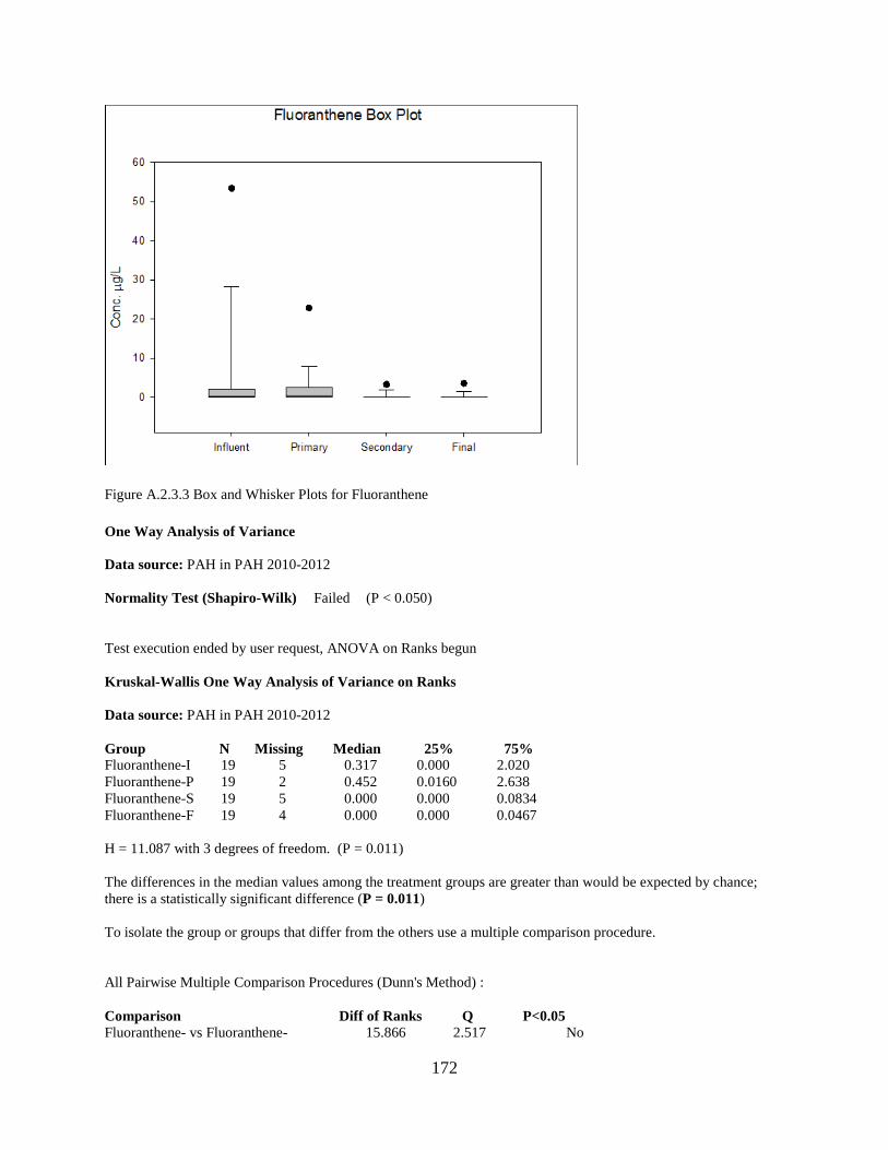
Figure A.2.3.3 Box and Whisker Plots for Fluoranthene One Way Analysis of Variance Data source: PAH in PAH 2010-2012 Normality Test (Shapiro-Wilk) Failed (P < 0.050) Test execution ended by user request, ANOVA on Ranks begun Kruskal-Wallis One Way Analysis of Variance on Ranks Data source: PAH in PAH 2010-2012 Group N Missing Median 25% 75% Fluoranthene-I 19 5 0.317 0.000 2.020 Fluoranthene-P 19 2 0.452 0.0160 2.638 Fluoranthene-S 19 5 0.000 0.000 0.0834 Fluoranthene-F 19 4 0.000 0.000 0.0467 H = 11.087 with 3 degrees of freedom. (P = 0.011) The differences in the median values among the treatment groups are greater than would be expected by chance; there is a statistically significant difference (P = 0.011) To isolate the group or groups that differ from the others use a multiple comparison procedure. All Pairwise Multiple Comparison Procedures (Dunn's Method) : Comparison Diff of Ranks Q P<0.05 Fluoranthene- vs Fluoranthene- 15.866 2.517 No
172

Fluoranthene- vs Fluoranthene- 14.627 2.364 Do Not Test Fluoranthene- vs Fluoranthene- 1.866 0.296 Do Not Test Mann-Whitney Rank Sum Test Data source: PAH in PAH 2010-2012 Normality Test (Shapiro-Wilk) Failed (P < 0.050) Group N Missing Median 25% 75% Fluoranthene-I 19 5 0.317 0.000 2.020 Fluoranthene-P 19 2 0.452 0.0160 2.638 Mann-Whitney U Statistic= 113.000 T = 218.000 n(small)= 14 n(big)= 17 (P = 0.826) The difference in the median values between the two groups is not great enough to exclude the possibility that the difference is due to random sampling variability; there is not a statistically significant difference (P = 0.826) Mann-Whitney Rank Sum Test Data source: PAH in PAH 2010-2012 Normality Test (Shapiro-Wilk) Failed (P < 0.050) Group N Missing Median 25% 75% Fluoranthene-P 19 2 0.452 0.0160 2.638 Fluoranthene-S 19 5 0.000 0.000 0.0834 Mann-Whitney U Statistic= 57.000 T = 162.000 n(small)= 14 n(big)= 17 (P = 0.011) The difference in the median values between the two groups is greater than would be expected by chance; there is a statistically significant difference (P = 0.011) Mann-Whitney Rank Sum Test Data source: PAH in PAH 2010-2012 Normality Test (Shapiro-Wilk) Failed (P < 0.050) Group N Missing Median 25% 75% Fluoranthene-S 19 5 0.000 0.000 0.0834 Fluoranthene-F 19 4 0.000 0.000 0.0467 Mann-Whitney U Statistic= 98.000 T = 203.000 n(small)= 14 n(big)= 15 (P = 0.751) The difference in the median values between the two groups is not great enough to exclude the possibility that the difference is due to random sampling variability; there is not a statistically significant difference (P = 0.751)
173

Mann-Whitney Rank Sum Test Data source: PAH in PAH 2010-2012 Normality Test (Shapiro-Wilk) Failed (P < 0.050) Group N Missing Median 25% 75% Fluoranthene-I 19 5 0.317 0.000 2.020 Fluoranthene-F 19 4 0.000 0.000 0.0467 Mann-Whitney U Statistic= 60.000 T = 255.000 n(small)= 14 n(big)= 15 (P = 0.044) The difference in the median values between the two groups is greater than would be expected by chance; there is a statistically significant difference (P = 0.044)
A.2.5. Summary Data for Acenaphthylene
Influent (µg/L)
After Primary (µg/L)
After Secondary (µg/L)
Final Effluent (µg/L)
Daily Flow (MGD)
Mass Influent (g/day)
Daily Rain Depth at Tuscaloosa airport (in)
Overall % Reduction
1/16/2010 56.6 0.0 0.0 0.0 18.2 3,895 0.55 100.0 3/2/2010 1.7 0.0 0.0 0.0 23.3 150 0.68 100.0 4/24/2010 4.7 3.9 4.0 4.6 16.5 292 1.01 1.9 6/25/2010 0.056 0.060 0.055 0.029 20.7 4 0.59 48.8 10/17/2010 0.29 4.2 0.0024 0.030 15.3 17 0.00 89.5 10.24/2010 0.2 0.3 0.2 0.0 15.7 9 0.10 81.4 11/2/2010 BQ 0.25 BQ BQ 20.5 0 0.88 0.0 3/9/2011 BQ 0.18 BQ x 42.2 0 2.67 0.0 5/11/2011 0.1 0.1 0.1 0.1 13.5 3 0.00 -50.5 9/20/2011 0.10 0.057 0.000 0.0042 26.5 10 0.64 95.8 10/10/2011 0.00 0.04 0.015 0.067 16.9 0 0.0 3/20/2012 0.12 0.27 0.050 0.057 17.1 8 0.00 50.7 6/16/2012 BDL BDL BDL BDL 13.5 0 0.00 0.0 9/15/2012 0.00 0.00 0.00 0.0 14.5 0 0.00 0.0 11/1/2012 0.00 0.00 0.00 0.0 17.1 0 0.00 0.0 11/4/2012 0.00 0.00 0.00 0.00 15.4 0 0.05 0.0 11/8/2012 BQ 0.00 0.00 0.00 15.9 0 0.00 0.0 11/12/2012 BQ BQ 0.00 0.00 16.0 0 0.44 0.0 Average dry (<0.1 inch of 0.08 0.58 0.01 0.02 17.95 3.74 0.01
8.98 (calc
174

rain) from avg)
Average wet
10.55 0.60 0.61 0.67 22.18 484.49 0.84
47.54 (calc from avg)
50250-25-50
99
90
50
10
15.02.50.0-2.5-5.0
99
90
50
10
1
420-2-4
99
90
50
10
1420-2-4
99
90
50
10
1
Influent_1
Perc
ent
Primary_1
Secondary_1 Final_1
Mean 4.906StDev 15.59N 13AD 3.903P-Value <0.005
Influent_1
Mean 0.5843StDev 1.355N 16AD 4.056P-Value <0.005
Primary_1
Mean 0.2945StDev 1.037N 15AD 4.792P-Value <0.005
Secondary_1
Mean 0.3269StDev 1.182N 15
Final_1
Normal - 95% CIAcenaphthylene
Figure A.2.5.1. Probability plot for Acenaphthylene
175

Figure A.2.5.2. Line graph for Acenaphthylene at four different sampling locations Column Size Missing Mean Std Dev Std. Error C.I. of Mean Acenaphthylene-I 19 6 4.906 15.591 4.324 9.422 Acenaphthylene-P 19 3 0.584 1.355 0.339 0.722 Acenaphthylene-S 19 4 0.294 1.037 0.268 0.574 Acenaphthylene-F 19 4 0.327 1.182 0.305 0.655 Column Range Max Min Median 25% 75% Acenaphthylene-I 56.612 56.612 0.000 0.101 0.000 0.642 Acenaphthylene-P 4.200 4.200 0.000 0.0584 0.000 0.257 Acenaphthylene-S 4.037 4.037 0.000 0.000 0.000 0.0511 Acenaphthylene-F 4.598 4.598 0.000 0.00423 0.000 0.0507 Column Skewness Kurtosis K-S Dist. K-S Prob. SWilk W SWilk Prob Acenaphthylene-I 3.562 12.764 0.429 <0.001 0.359 <0.001 Acenaphthylene-P 2.486 4.868 0.445 <0.001 0.470 <0.001 Acenaphthylene-S 3.855 14.900 0.467 <0.001 0.315 <0.001 Acenaphthylene-F 3.869 14.978 0.513 <0.001 0.303 <0.001
0.0
0.0
0.1
1.0
10.0
100.0
Influent Primary Secondary Final
Conc
entr
atio
n (μ
g/L)
Acenaphythylene
01/16/2010 (w)
3/2/2010 (w)
4/24/2010 (w)
6/25/2010 (w)
10/17/2010 (d)
10/24/2010 (w)
11/2/2010 (w)
3/9/2010 (w)
5/11/2011 (d)
9/20/2011 (w)
10/10/2011 (d)
3/20/2012 (d)
176

Column Sum Sum of Squares Acenaphthylene-I 63.778 3229.911 Acenaphthylene-P 9.349 32.987 Acenaphthylene-S 4.417 16.348 Acenaphthylene-F 4.904 21.162
Figure A.2.5.1. Box and Whisker Plots for Acenaphthylene One Way Analysis of Variance Data source: PAH in PAH 2010-2012 Normality Test (Shapiro-Wilk) Failed (P < 0.050) Test execution ended by user request, ANOVA on Ranks begun Kruskal-Wallis One Way Analysis of Variance on Ranks Wednesday, January 16, 2013, 12:30:57 PM Data source: PAH in PAH 2010-2012 Group N Missing Median 25% 75% Acenaphthylene-I 19 6 0.101 0.000 0.994 Acenaphthylene-P 19 3 0.0584 0.000 0.263 Acenaphthylene-S 19 4 0.000 0.000 0.0516 Acenaphthylene-F 19 4 0.00423 0.000 0.0575 H = 6.008 with 3 degrees of freedom. (P = 0.111) The differences in the median values among the treatment groups are not great enough to exclude the possibility that the difference is due to random sampling variability; there is not a statistically significant difference (P = 0.111)
177

Mann-Whitney Rank Sum Test Data source: PAH in PAH 2010-2012 Normality Test (Shapiro-Wilk) Failed (P < 0.050) Group N Missing Median 25% 75% Acenaphthylene-I 19 6 0.101 0.000 0.994 Acenaphthylene-P 19 3 0.0584 0.000 0.263 Mann-Whitney U Statistic= 92.000 T = 207.000 n(small)= 13 n(big)= 16 (P = 0.607) The difference in the median values between the two groups is not great enough to exclude the possibility that the difference is due to random sampling variability; there is not a statistically significant difference (P = 0.607) Mann-Whitney Rank Sum Test Data source: PAH in PAH 2010-2012 Normality Test (Shapiro-Wilk) Failed (P < 0.050) Group N Missing Median 25% 75% Acenaphthylene-P 19 3 0.0584 0.000 0.263 Acenaphthylene-S 19 4 0.000 0.000 0.0516 Mann-Whitney U Statistic= 83.000 T = 203.000 n(small)= 15 n(big)= 16 (P = 0.130) The difference in the median values between the two groups is not great enough to exclude the possibility that the difference is due to random sampling variability; there is not a statistically significant difference (P = 0.130) Mann-Whitney Rank Sum Test Data source: PAH in PAH 2010-2012 Normality Test (Shapiro-Wilk) Failed (P < 0.050) Group N Missing Median 25% 75% Acenaphthylene-S 19 4 0.000 0.000 0.0516 Acenaphthylene-F 19 4 0.00423 0.000 0.0575 Mann-Whitney U Statistic= 104.000 T = 224.000 n(small)= 15 n(big)= 15 (P = 0.723) The difference in the median values between the two groups is not great enough to exclude the possibility that the difference is due to random sampling variability; there is not a statistically significant difference (P = 0.723) Mann-Whitney Rank Sum Test
178

Data source: PAH in PAH 2010-2012 Normality Test (Shapiro-Wilk) Failed (P < 0.050) Group N Missing Median 25% 75% Acenaphthylene-I 19 6 0.101 0.000 0.994 Acenaphthylene-F 19 4 0.00423 0.000 0.0575 Mann-Whitney U Statistic= 58.000 T = 228.000 n(small)= 13 n(big)= 15 (P = 0.064) The difference in the median values between the two groups is not great enough to exclude the possibility that the difference is due to random sampling variability; there is not a statistically significant difference (P = 0.064)
A.2.6. Summary Data for Phenanthrene
Influent (µg/L)
After Primary (µg/L)
After Secondary (µg/L)
Final Effluent (µg/L)
Daily Flow (MGD)
Mass Influent (g/day)
Daily Rain Depth at Tuscaloosa airport (in)
Overall % Reduction
1/16/2010 40.9 20.2 0.0 0.0 18.2 2752.4 0.55 100.0 3/2/2010 1.2 0.6 0.0 0.0 23.3 105.7 0.68 100.0 4/24/2010 0.0 0.0 0.0 0.0 16.5 0.0 1.01 0.0 6/25/2010 BQ BQ BQ BQ 20.7 0.0 0.59 0.0 10/17/2010 4.9 14 0.043 0.61 15.3 280.1 0.00 87.7 10.24/2010 0.0 0.0 0.0 0.0 15.7 0.0 0.10 0.0 11/2/2010 0.40 2.9 0.19 0.24 20.5 30.0 0.88 38.5 3/9/2011 0.30 6.4 BQ n/a 42.2 46.1 2.67 100.0 5/11/2011 2.8 2.8 0.0 0.0 13.5 137.5 0.00 100.0 5/14/2011 2.3 1.8 BQ BQ 30.7 258.6 0.00 100.0 9/20/2011 0.19 0.35 0.000 0.019 26.5 18.5 0.64 89.9 10/10/2011 0.14 0.54 0.045 0.043 16.9 8.5 0.00 68.0 3/20/2012 1.4 3.6 1.1 0.69 17.1 88.2 0.00 50.8 6/16/2012 0.09 0.41 0.065 BDL 13.5 4.4 0.00 100.0 9/15/2012 0.00 0.00 0.00 0.0 14.5 0.0 0.00 0.0 11/1/2012 0.00 0.000 0.000 0.0 17.1 0.0 0.00 0.0 11/4/2012 0.00 0.00 0.00 0.00 15.4 0.0 0.05 0.0 11/8/2012 3.9 0.00 0.00 0.00 15.9 231.3 0.00 100.0 11/12/2012 BQ BQ 0.00 0.00 16.0 0.0 0.44 0.0 Average dry (<0.1 inch of rain)
1.56 0.77 0.16 0.12 18.84 75.13 0.01
53.55 (calc from avg)
179

Average wet
6.14 4.36 0.05 0.15 20.10 62.77 0.84
47.60 (calc from avg)
40200-20
99
90
50
10
120100-10-20
99
90
50
10
1
1.00.50.0-0.5-1.0
99
90
50
10
11.00.50.0-0.5
99
90
50
10
1
Influent_2
Perc
ent
Primary_2
Secondary_2 Final_2
Mean 3.442StDev 9.765N 17AD 4.358P-Value <0.005
Influent_2
Mean 3.122StDev 5.584N 17AD 2.585P-Value <0.005
Primary_2
Mean 0.08902StDev 0.2696N 16AD 4.316P-Value <0.005
Secondary_2
Mean 0.1068StDev 0.2287N 15
Final_2
Normal - 95% CIPhenanthrene
Figure A.2.6. 1. Probability plot for Phenanthrene
180

Figure A.2.6.2 Line graph for Phenanthrene at four different sampling locations Column Size Missing Mean Std Dev Std. Error C.I. of Mean Phenanthrene-I 19 2 3.442 9.765 2.368 5.021 Phenanthrene-P 19 2 3.122 5.584 1.354 2.871 Phenanthrene-S 19 3 0.0890 0.270 0.0674 0.144 Phenanthrene-F 19 4 0.107 0.229 0.0591 0.127 Column Range Max Min Median 25% 75% Phenanthrene-I 40.873 40.873 0.000 0.295 0.000 2.396 Phenanthrene-P 20.179 20.179 0.000 0.538 0.000 3.064 Phenanthrene-S 1.083 1.083 0.000 0.000 0.000 0.0439 Phenanthrene-F 0.686 0.686 0.000 0.000 0.000 0.0372 Column Skewness Kurtosis K-S Dist. K-S Prob. SWilk W SWilk Prob Phenanthrene-I 3.960 16.018 0.380 <0.001 0.379 <0.001 Phenanthrene-P 2.388 5.460 0.290 <0.001 0.625 <0.001 Phenanthrene-S 3.795 14.739 0.411 <0.001 0.377 <0.001 Phenanthrene-F 2.140 3.378 0.409 <0.001 0.535 <0.001 Column Sum Sum of Squares Phenanthrene-I 58.507 1727.075 Phenanthrene-P 53.075 664.664 Phenanthrene-S 1.424 1.217 Phenanthrene-F 1.601 0.904 One Way Analysis of Variance
0.0
0.1
1.0
10.0
100.0
Influent Primary Secondary Final
Conc
entr
atio
nn (μ
g/L)
Phenanthrene
01/16/2010 (w)
3/2/2010 (w)
10/17/2010 (d)
11/2/2010 (w)
3/9/2010 (w)
5/11/2011 (d)
5/14/2011 (d)
9/20/2011 (w)
10/10/2011 (d)
3/20/2012 (d)
6/16/2012 (d)
181
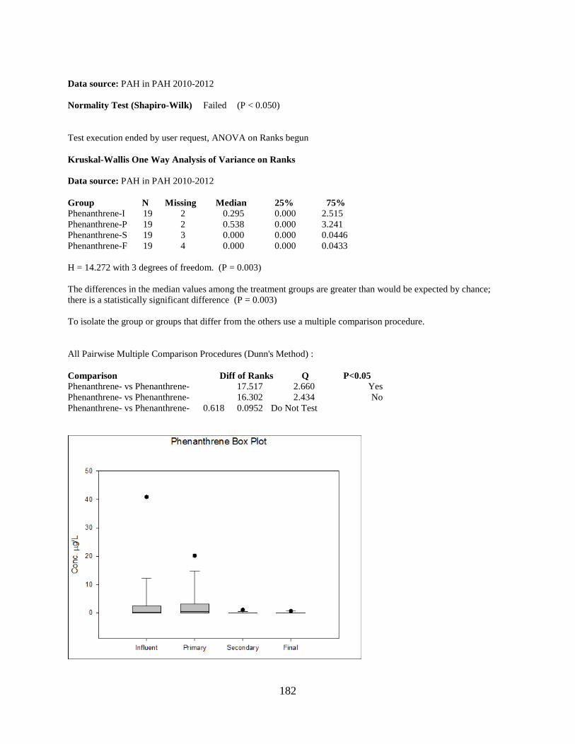
Data source: PAH in PAH 2010-2012 Normality Test (Shapiro-Wilk) Failed (P < 0.050) Test execution ended by user request, ANOVA on Ranks begun Kruskal-Wallis One Way Analysis of Variance on Ranks Data source: PAH in PAH 2010-2012 Group N Missing Median 25% 75% Phenanthrene-I 19 2 0.295 0.000 2.515 Phenanthrene-P 19 2 0.538 0.000 3.241 Phenanthrene-S 19 3 0.000 0.000 0.0446 Phenanthrene-F 19 4 0.000 0.000 0.0433 H = 14.272 with 3 degrees of freedom. (P = 0.003) The differences in the median values among the treatment groups are greater than would be expected by chance; there is a statistically significant difference (P = 0.003) To isolate the group or groups that differ from the others use a multiple comparison procedure. All Pairwise Multiple Comparison Procedures (Dunn's Method) : Comparison Diff of Ranks Q P<0.05 Phenanthrene- vs Phenanthrene- 17.517 2.660 Yes Phenanthrene- vs Phenanthrene- 16.302 2.434 No Phenanthrene- vs Phenanthrene- 0.618 0.0952 Do Not Test
182
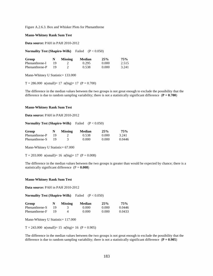
Figure A.2.6.3. Box and Whisker Plots for Phenanthrene Mann-Whitney Rank Sum Test Data source: PAH in PAH 2010-2012 Normality Test (Shapiro-Wilk) Failed (P < 0.050) Group N Missing Median 25% 75% Phenanthrene-I 19 2 0.295 0.000 2.515 Phenanthrene-P 19 2 0.538 0.000 3.241 Mann-Whitney U Statistic= 133.000 T = 286.000 n(small)= 17 n(big)= 17 (P = 0.700) The difference in the median values between the two groups is not great enough to exclude the possibility that the difference is due to random sampling variability; there is not a statistically significant difference (P = 0.700) Mann-Whitney Rank Sum Test Data source: PAH in PAH 2010-2012 Normality Test (Shapiro-Wilk) Failed (P < 0.050) Group N Missing Median 25% 75% Phenanthrene-P 19 2 0.538 0.000 3.241 Phenanthrene-S 19 3 0.000 0.000 0.0446 Mann-Whitney U Statistic= 67.000 T = 203.000 n(small)= 16 n(big)= 17 (P = 0.008) The difference in the median values between the two groups is greater than would be expected by chance; there is a statistically significant difference (P = 0.008) Mann-Whitney Rank Sum Test Data source: PAH in PAH 2010-2012 Normality Test (Shapiro-Wilk) Failed (P < 0.050) Group N Missing Median 25% 75% Phenanthrene-S 19 3 0.000 0.000 0.0446 Phenanthrene-F 19 4 0.000 0.000 0.0433 Mann-Whitney U Statistic= 117.000 T = 243.000 n(small)= 15 n(big)= 16 (P = 0.905) The difference in the median values between the two groups is not great enough to exclude the possibility that the difference is due to random sampling variability; there is not a statistically significant difference (P = 0.905)
183

Mann-Whitney Rank Sum Test Data source: PAH in PAH 2010-2012 Normality Test (Shapiro-Wilk) Failed (P < 0.050) Group N Missing Median 25% 75% Phenanthrene-I 19 2 0.295 0.000 2.515 Phenanthrene-F 19 4 0.000 0.000 0.0433 Mann-Whitney U Statistic= 63.000 T = 183.000 n(small)= 15 n(big)= 17 (P = 0.011) The difference in the median values between the two groups is greater than would be expected by chance; there is a statistically significant difference (P = 0.011)
A.2.7. Summary Data for Anthracene
Influent (µg/L)
After Primary (µg/L)
After Secondary (µg/L)
Final Effluent (µg/L)
Daily Flow (MGD)
Mass Influent (g/day)
Daily Rain Depth at Tuscaloosa airport (in)
Overall % Reduction
1/16/2010 54.5 0.0 69.1 0.0 18.2 3669.2 0.55 100.0 3/2/2010 1.6 0.0 2.1 0.0 23.3 110.1 0.68 100.0 4/24/2010 3.8 2.7 4.1 4.1 16.5 255.2 1.01 -7.2 6/25/2010 0.096 0.087 0.11 0.049 20.7 6.5 0.59 48.8 10/17/2010 478 0.90 BQ 0.20 15.3 32166.9 0.00 100.0 10.24/2010 1124.8 9.5 2.2 1.5 15.7 75742.0 0.10 99.9 11/2/2010 BQ 0.10 0.11 BQ 20.5 0.0 0.88 0.0 3/9/2011 BQ 5.6 BQ n/a 42.2 0.0 2.67 0.0 5/11/2011 1.7 0.0 1.0 0.9 13.5 117.6 0.00 47.2 5/14/2011 0.8 0.4 1.1 BQ 30.7 55.4 0.00 100.0 9/20/2011 0.10 0.19 0.000 0.13 26.5 6.6 0.64 -34.7 10/10/2011 0.01 0.39 0.061 0.18 16.9 0.8 0.00 -1345.8 3/20/2012 0.19 0.08 0.060 0.037 17.1 12.9 0.00 80.7 6/16/2012 BDL BDL 0.0068 0.062 13.5 0.0 0.00 0.0 9/15/2012 0.00 0.00 0.00 0.000 14.5 0.0 0.00 0.0 11/1/2012 0.00 0.000 0.0000 0.000 17.1 0.0 0.00 0.0 11/4/2012 0.00 0.00 0.00 0.00 15.4 0.0 0.05 0.0 11/8/2012 BQ 0.00 0.00 0.00 15.9 0.0 0.00 0.0 11/12/2012 BQ BQ 0.00 0.00 16.0 0.0 0.44 0.0 Average dry (<0.1 inch of rain) 60.07 0.18 0.24 0.15 17.95 3,235.94 0.01
-101.80 (calc from
184

avg) Average wet
197.48 2.27 9.70 0.81 22.18 8,865.52 0.84
34.09 (calc from avg)
10005000-500-1000
99
90
50
10
11050-5
99
90
50
10
1
500-50
99
90
50
10
1420-2-4
99
90
50
10
1
Influent_2_1
Perc
ent
Primary_2_1
Secondary_2_1 Final_2_1
Mean 119.0StDev 316.0N 14AD 3.612P-Value <0.005
Influent_2_1
Mean 1.173StDev 2.577N 17AD 3.490P-Value <0.005
Primary_2_1
Mean 4.698StDev 16.64N 17AD 5.301P-Value <0.005
Secondary_2_1
Mean 0.4432StDev 1.046N 16
Final_2_1
Normal - 95% CIAnthracene
Figure A.2.7.1 Probability Plot for Anthracene
185

Figure A.2.7.2. Line graph for Anthracene at four different sampling locations Column Size Missing Mean Std Dev Std. Error C.I. of Mean Anthracene-I 19 5 118.952 316.006 84.456 182.457 Anthracene-P 19 2 1.173 2.577 0.625 1.325 Anthracene-S 19 2 4.698 16.641 4.036 8.556 Anthracene-F 19 3 0.443 1.046 0.261 0.557 Column Range Max Min Median 25% 75% Anthracene-I 1124.770 1124.770 0.000 0.507 0.0123 3.790 Anthracene-P 9.490 9.490 0.000 0.0867 0.000 0.534 Anthracene-S 69.125 69.125 0.000 0.0605 0.000 1.368 Anthracene-F 4.062 4.062 0.000 0.0431 0.000 0.188 Column Skewness Kurtosis K-S Dist. K-S Prob. SWilk W SWilk Prob Anthracene-I 2.973 8.949 0.438 <0.001 0.449 <0.001 Anthracene-P 2.676 7.042 0.381 <0.001 0.533 <0.001 Anthracene-S 4.091 16.811 0.456 <0.001 0.308 <0.001 Anthracene-F 3.174 10.691 0.405 <0.001 0.493 <0.001 Column Sum Sum of Squares Anthracene-I 1665.329 1496274.755 Anthracene-P 19.942 129.638 Anthracene-S 79.869 4806.004 Anthracene-F 7.091 19.549
0.0
0.0
0.1
1.0
10.0
100.0
1000.0
10000.0
Influent Primary Secondary Final
Conc
entr
atio
n (μ
g/L)
Anthracene
01/16/2010 (w)
3/2/2010 (w)
4/24/2010 (w)
6/25/2010 (w)
10/17/2010 (d)
10/24/2010 (w)
11/2/2010 (w)
3/9/2010 (w)
5/11/2011 (d)
5/14/2011 (d)
9/20/2011 (w)
10/10/2011 (d)
3/20/2012 (d)
186

Figure A.2.7.3 Box and Whisker Plots for Anthracene One Way Analysis of Variance Data source: PAH in PAH 2010-2012 Normality Test (Shapiro-Wilk) Failed (P < 0.050) Test execution ended by user request, ANOVA on Ranks begun Kruskal-Wallis One Way Analysis of Variance on Ranks Data source: PAH in PAH 2010-2012 Group N Missing Median 25% 75% Anthracene-I 19 5 0.507 0.00922 16.465 Anthracene-P 19 2 0.0867 0.000 0.655 Anthracene-S 19 2 0.0605 0.000 1.603 Anthracene-F 19 3 0.0431 0.000 0.193 H = 3.737 with 3 degrees of freedom. (P = 0.291) The differences in the median values among the treatment groups are not great enough to exclude the possibility that the difference is due to random sampling variability; there is not a statistically significant difference (P = 0.291) Mann-Whitney Rank Sum Test Data source: PAH in PAH 2010-2012 Normality Test (Shapiro-Wilk) Failed (P < 0.050)
187

Group N Missing Median 25% 75% Anthracene-I 19 5 0.507 0.00922 16.465 Anthracene-P 19 2 0.0867 0.000 0.655 Mann-Whitney U Statistic= 84.500 T = 258.500 n(small)= 14 n(big)= 17 (P = 0.170) The difference in the median values between the two groups is not great enough to exclude the possibility that the difference is due to random sampling variability; there is not a statistically significant difference (P = 0.170) Mann-Whitney Rank Sum Test Data source: PAH in PAH 2010-2012 Normality Test (Shapiro-Wilk) Failed (P < 0.050) Group N Missing Median 25% 75% Anthracene-P 19 2 0.0867 0.000 0.655 Anthracene-S 19 2 0.0605 0.000 1.603 Mann-Whitney U Statistic= 139.000 T = 292.000 n(small)= 17 n(big)= 17 (P = 0.859) The difference in the median values between the two groups is not great enough to exclude the possibility that the difference is due to random sampling variability; there is not a statistically significant difference (P = 0.859) Mann-Whitney Rank Sum Test Data source: PAH in PAH 2010-2012 Normality Test (Shapiro-Wilk) Failed (P < 0.050) Group N Missing Median 25% 75% Anthracene-S 19 2 0.0605 0.000 1.603 Anthracene-F 19 3 0.0431 0.000 0.193 Mann-Whitney U Statistic= 116.000 T = 252.000 n(small)= 16 n(big)= 17 (P = 0.469) The difference in the median values between the two groups is not great enough to exclude the possibility that the difference is due to random sampling variability; there is not a statistically significant difference (P = 0.469) Mann-Whitney Rank Sum Test Data source: PAH in PAH 2010-2012 Normality Test (Shapiro-Wilk) Failed (P < 0.050) Group N Missing Median 25% 75% Anthracene-I 19 5 0.507 0.00922 16.465
188
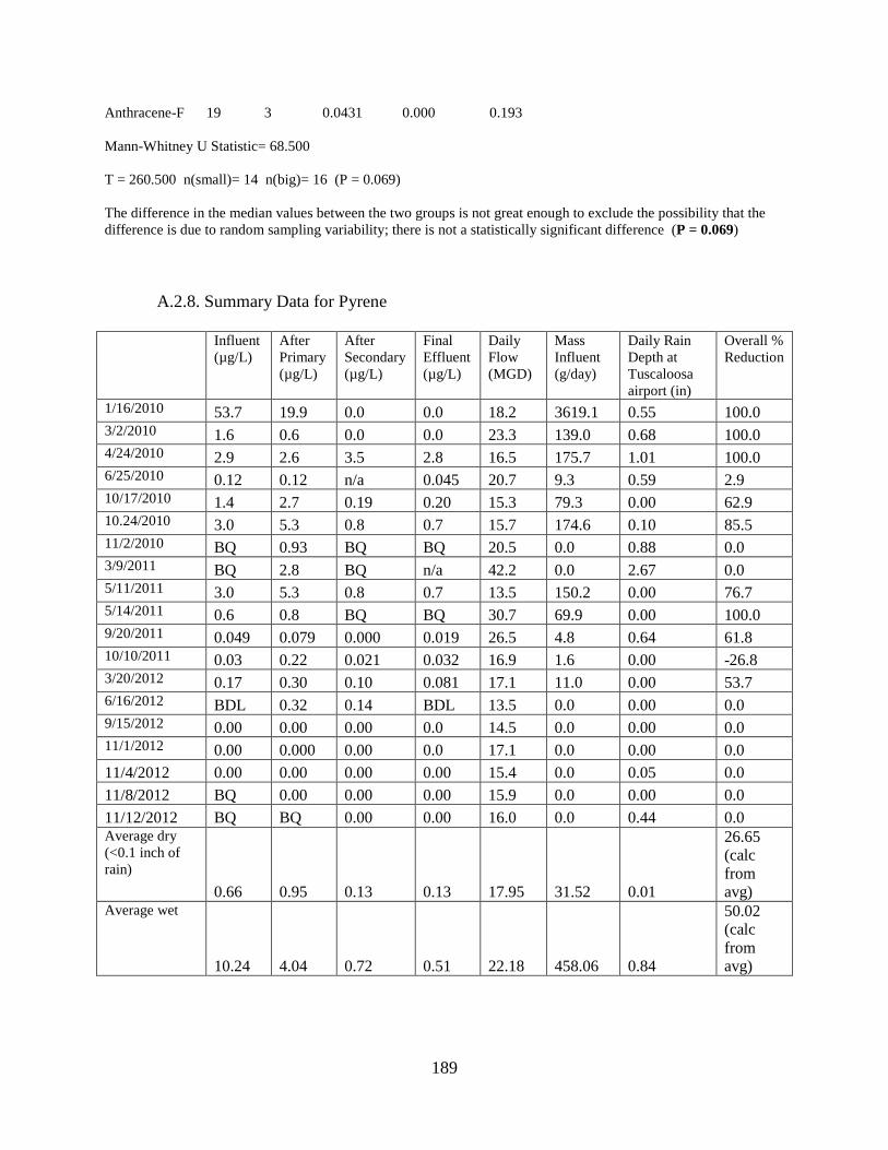
Anthracene-F 19 3 0.0431 0.000 0.193 Mann-Whitney U Statistic= 68.500 T = 260.500 n(small)= 14 n(big)= 16 (P = 0.069) The difference in the median values between the two groups is not great enough to exclude the possibility that the difference is due to random sampling variability; there is not a statistically significant difference (P = 0.069)
A.2.8. Summary Data for Pyrene
Influent (µg/L)
After Primary (µg/L)
After Secondary (µg/L)
Final Effluent (µg/L)
Daily Flow (MGD)
Mass Influent (g/day)
Daily Rain Depth at Tuscaloosa airport (in)
Overall % Reduction
1/16/2010 53.7 19.9 0.0 0.0 18.2 3619.1 0.55 100.0 3/2/2010 1.6 0.6 0.0 0.0 23.3 139.0 0.68 100.0 4/24/2010 2.9 2.6 3.5 2.8 16.5 175.7 1.01 100.0 6/25/2010 0.12 0.12 n/a 0.045 20.7 9.3 0.59 2.9 10/17/2010 1.4 2.7 0.19 0.20 15.3 79.3 0.00 62.9 10.24/2010 3.0 5.3 0.8 0.7 15.7 174.6 0.10 85.5 11/2/2010 BQ 0.93 BQ BQ 20.5 0.0 0.88 0.0 3/9/2011 BQ 2.8 BQ n/a 42.2 0.0 2.67 0.0 5/11/2011 3.0 5.3 0.8 0.7 13.5 150.2 0.00 76.7 5/14/2011 0.6 0.8 BQ BQ 30.7 69.9 0.00 100.0 9/20/2011 0.049 0.079 0.000 0.019 26.5 4.8 0.64 61.8 10/10/2011 0.03 0.22 0.021 0.032 16.9 1.6 0.00 -26.8 3/20/2012 0.17 0.30 0.10 0.081 17.1 11.0 0.00 53.7 6/16/2012 BDL 0.32 0.14 BDL 13.5 0.0 0.00 0.0 9/15/2012 0.00 0.00 0.00 0.0 14.5 0.0 0.00 0.0 11/1/2012 0.00 0.000 0.00 0.0 17.1 0.0 0.00 0.0 11/4/2012 0.00 0.00 0.00 0.00 15.4 0.0 0.05 0.0 11/8/2012 BQ 0.00 0.00 0.00 15.9 0.0 0.00 0.0 11/12/2012 BQ BQ 0.00 0.00 16.0 0.0 0.44 0.0 Average dry (<0.1 inch of rain)
0.66 0.95 0.13 0.13 17.95 31.52 0.01
26.65 (calc from avg)
Average wet
10.24 4.04 0.72 0.51 22.18 458.06 0.84
50.02 (calc from avg)
189

50250-25-50
99
90
50
10
120100-10
99
90
50
10
1
420-2
99
90
50
10
120-2
99
90
50
10
1
Influent_2_2
Perc
ent
Primary_2_2
Secondary_2_2 Final_2_2
Mean 4.759StDev 14.15N 14AD 4.005P-Value <0.005
Influent_2_2
Mean 2.330StDev 4.714N 18AD 3.023P-Value <0.005
Primary_2_2
Mean 0.3668StDev 0.9161N 15AD 3.337P-Value <0.005
Secondary_2_2
Mean 0.3050StDev 0.7293N 15
Final_2_2
Normal - 95% CIPyrene
Figure A.2.8.1. Probability plots for Pyrene
0.0
0.1
1.0
10.0
100.0
Influent Primary Secondary Final
Conc
entr
atio
n (μ
g/L)
Pyrene
01/16/2010 (w)
3/2/2010 (w)
4/24/2010 (w)
6/25/2010 (w)
10/17/2010 (d)
10/24/2010 (w)
11/2/2010 (w)
3/9/2010 (w)
5/14/2011 (d)
9/20/2011 (w)
10/10/2011 (d)
3/20/2012 (d)
190

Figure A.2.8.2 Line graphs for Pyrene at four different sampling locations Column Size Missing Mean Std Dev Std. Error C.I. of Mean Pyrene-I 19 5 4.759 14.149 3.782 8.170 Pyrene-P 19 1 2.330 4.714 1.111 2.344 Pyrene-S 19 4 0.367 0.916 0.237 0.507 Pyrene-F 19 4 0.305 0.729 0.188 0.404 Column Range Max Min Median 25% 75% Pyrene-I 53.744 53.744 0.000 0.395 0.0252 2.878 Pyrene-P 19.868 19.868 0.000 0.458 0.0791 2.663 Pyrene-S 3.545 3.545 0.000 0.000 0.000 0.177 Pyrene-F 2.794 2.794 0.000 0.0187 0.000 0.173 Column Skewness Kurtosis K-S Dist. K-S Prob. SWilk W SWilk Prob Pyrene-I 3.696 13.751 0.478 <0.001 0.364 <0.001 Pyrene-P 3.371 12.508 0.311 <0.001 0.531 <0.001 Pyrene-S 3.404 12.186 0.377 <0.001 0.461 <0.001 Pyrene-F 3.247 11.204 0.355 <0.001 0.485 <0.001 Column Sum Sum of Squares Pyrene-I 66.632 2919.771 Pyrene-P 41.939 475.567 Pyrene-S 5.502 13.769 Pyrene-F 4.575 8.841
Figure A.2.8.3. Box and Whisker Plots for Pyrene
191
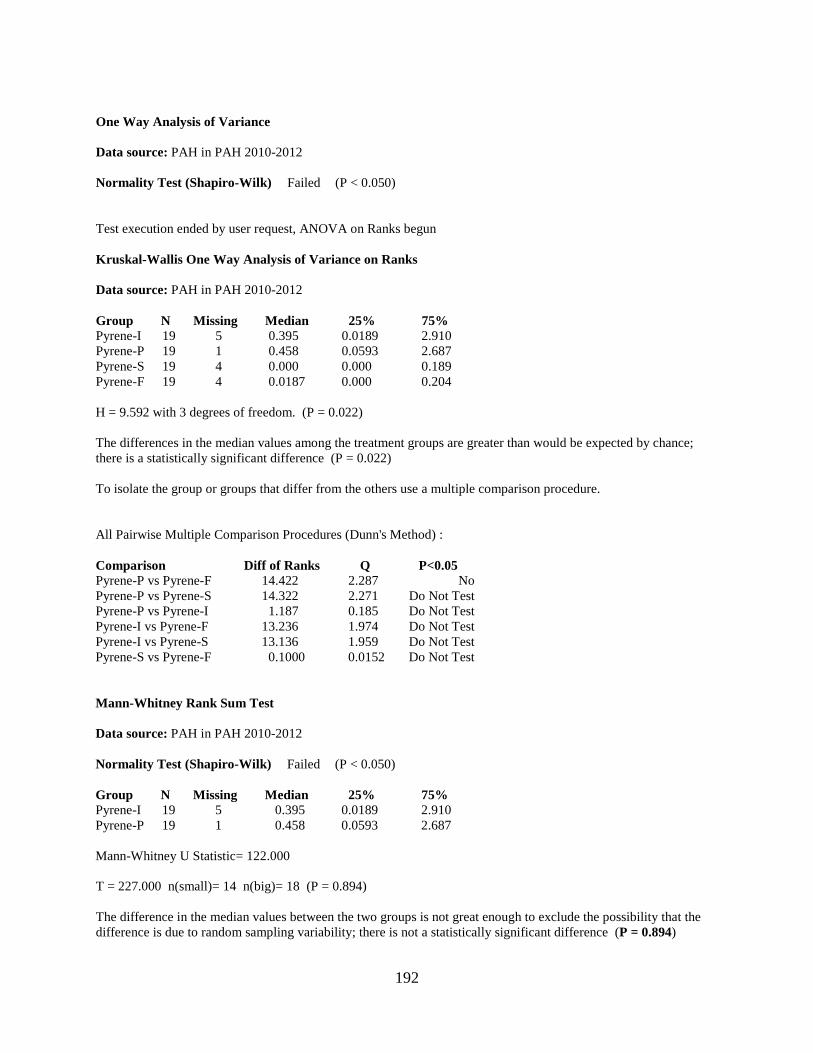
One Way Analysis of Variance Data source: PAH in PAH 2010-2012 Normality Test (Shapiro-Wilk) Failed (P < 0.050) Test execution ended by user request, ANOVA on Ranks begun Kruskal-Wallis One Way Analysis of Variance on Ranks Data source: PAH in PAH 2010-2012 Group N Missing Median 25% 75% Pyrene-I 19 5 0.395 0.0189 2.910 Pyrene-P 19 1 0.458 0.0593 2.687 Pyrene-S 19 4 0.000 0.000 0.189 Pyrene-F 19 4 0.0187 0.000 0.204 H = 9.592 with 3 degrees of freedom. (P = 0.022) The differences in the median values among the treatment groups are greater than would be expected by chance; there is a statistically significant difference (P = 0.022) To isolate the group or groups that differ from the others use a multiple comparison procedure. All Pairwise Multiple Comparison Procedures (Dunn's Method) : Comparison Diff of Ranks Q P<0.05 Pyrene-P vs Pyrene-F 14.422 2.287 No Pyrene-P vs Pyrene-S 14.322 2.271 Do Not Test Pyrene-P vs Pyrene-I 1.187 0.185 Do Not Test Pyrene-I vs Pyrene-F 13.236 1.974 Do Not Test Pyrene-I vs Pyrene-S 13.136 1.959 Do Not Test Pyrene-S vs Pyrene-F 0.1000 0.0152 Do Not Test Mann-Whitney Rank Sum Test Data source: PAH in PAH 2010-2012 Normality Test (Shapiro-Wilk) Failed (P < 0.050) Group N Missing Median 25% 75% Pyrene-I 19 5 0.395 0.0189 2.910 Pyrene-P 19 1 0.458 0.0593 2.687 Mann-Whitney U Statistic= 122.000 T = 227.000 n(small)= 14 n(big)= 18 (P = 0.894) The difference in the median values between the two groups is not great enough to exclude the possibility that the difference is due to random sampling variability; there is not a statistically significant difference (P = 0.894)
192

Mann-Whitney Rank Sum Test Data source: PAH in PAH 2010-2012 Normality Test (Shapiro-Wilk) Failed (P < 0.050) Group N Missing Median 25% 75% Pyrene-P 19 1 0.458 0.0593 2.687 Pyrene-S 19 4 0.000 0.000 0.189 Mann-Whitney U Statistic= 72.000 T = 192.000 n(small)= 15 n(big)= 18 (P = 0.021) The difference in the median values between the two groups is greater than would be expected by chance; there is a statistically significant difference (P = 0.021) Mann-Whitney Rank Sum Test Data source: PAH in PAH 2010-2012 Normality Test (Shapiro-Wilk) Failed (P < 0.050) Group N Missing Median 25% 75% Pyrene-S 19 4 0.000 0.000 0.189 Pyrene-F 19 4 0.0187 0.000 0.204 Mann-Whitney U Statistic= 112.000 T = 232.000 n(small)= 15 n(big)= 15 (P = 1.000) The difference in the median values between the two groups is not great enough to exclude the possibility that the difference is due to random sampling variability; there is not a statistically significant difference (P = 1.000) Mann-Whitney Rank Sum Test Data source: PAH in PAH 2010-2012 Normality Test (Shapiro-Wilk) Failed (P < 0.050) Group N Missing Median 25% 75% Pyrene-I 19 5 0.395 0.0189 2.910 Pyrene-F 19 4 0.0187 0.000 0.204 Mann-Whitney U Statistic= 59.500 T = 255.500 n(small)= 14 n(big)= 15 (P = 0.045) The difference in the median values between the two groups is greater than would be expected by chance; there is a statistically significant difference (P = 0.045)
193

A.2.9. Benzo(a)anthracene plus chrysene A.2.10. Benzo(b)fluoranthene, benzo(k)fluoranthene, benzo(a)pyrene, and indeno(1,2,3,cd)pyrene A.2.11. Benzo(a,h)anthracene plus benzo(g,h,i) perylene
A.3. Pesticides
194

APPENDIX B: CHROMATOGRAPHS FOR SAMPLE ANALYSES
Figure B.1. Influent Sample for 11/08/12: Acid Group I
Figure B.2. Influent Sample for 11/08/12: Acid Group II
195
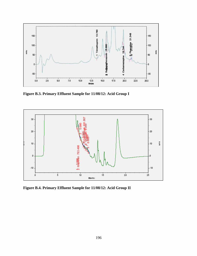
Figure B.3. Primary Effluent Sample for 11/08/12: Acid Group I
Figure B.4. Primary Effluent Sample for 11/08/12: Acid Group II
196
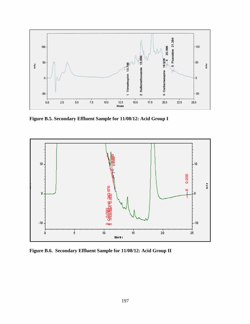
Figure B.5. Secondary Effluent Sample for 11/08/12: Acid Group I
Figure B.6. Secondary Effluent Sample for 11/08/12: Acid Group II
197
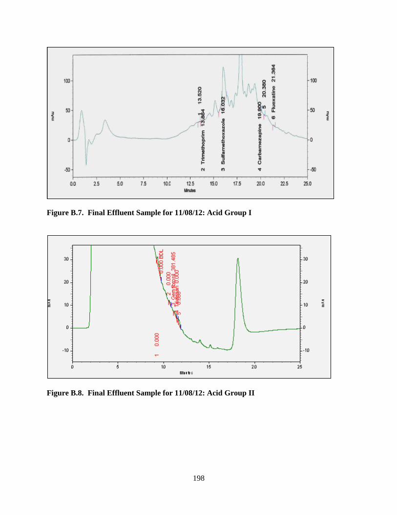
Figure B.7. Final Effluent Sample for 11/08/12: Acid Group I
Figure B.8. Final Effluent Sample for 11/08/12: Acid Group II
198
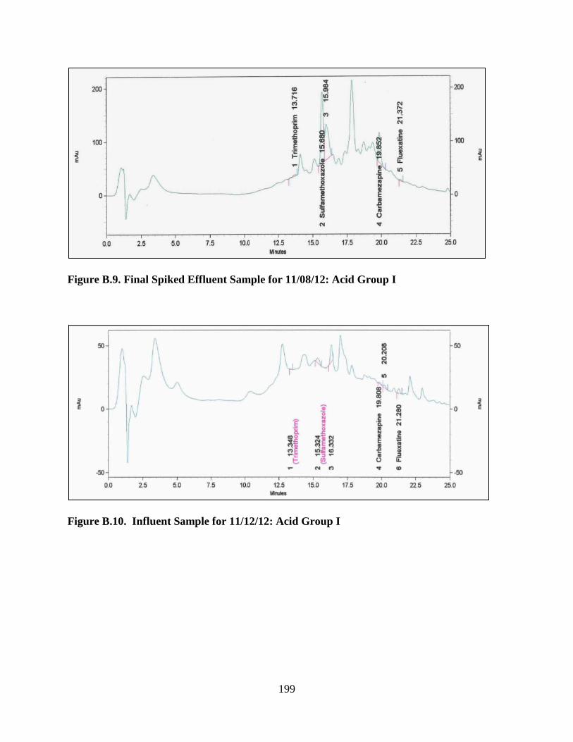
Figure B.9. Final Spiked Effluent Sample for 11/08/12: Acid Group I
Figure B.10. Influent Sample for 11/12/12: Acid Group I
199
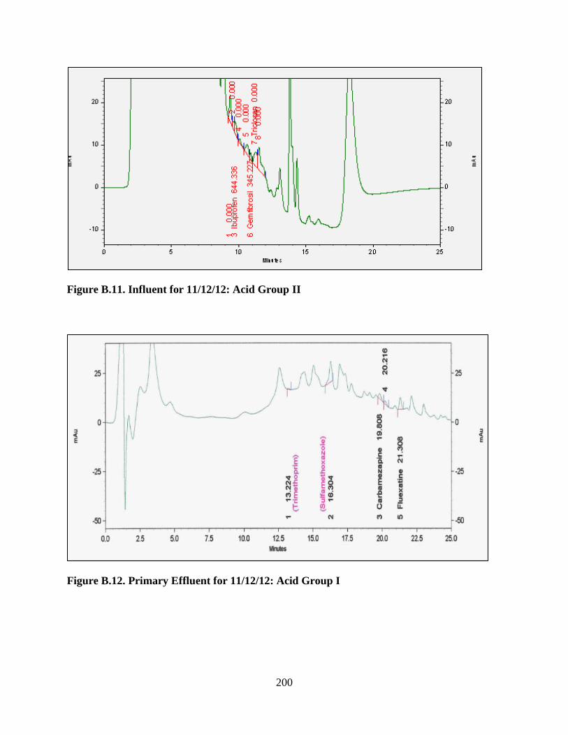
Figure B.11. Influent for 11/12/12: Acid Group II
Figure B.12. Primary Effluent for 11/12/12: Acid Group I
200

Figure B.13. Primary Effluent for 11/12/12: Acid Group II
Figure B.14. Secondary Effluent for 11/12/12: Acid Group I
201
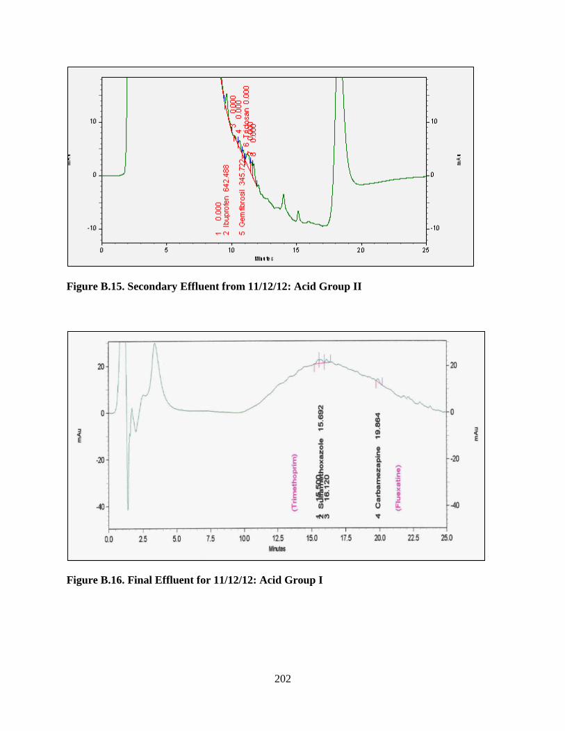
Figure B.15. Secondary Effluent from 11/12/12: Acid Group II
Figure B.16. Final Effluent for 11/12/12: Acid Group I
202

Figure B.17. Final Effluent from 11/12/12: Acid Group II
Figure B.18. Final Effluent (Spiked) for 11/12/12: Acid Group I
203
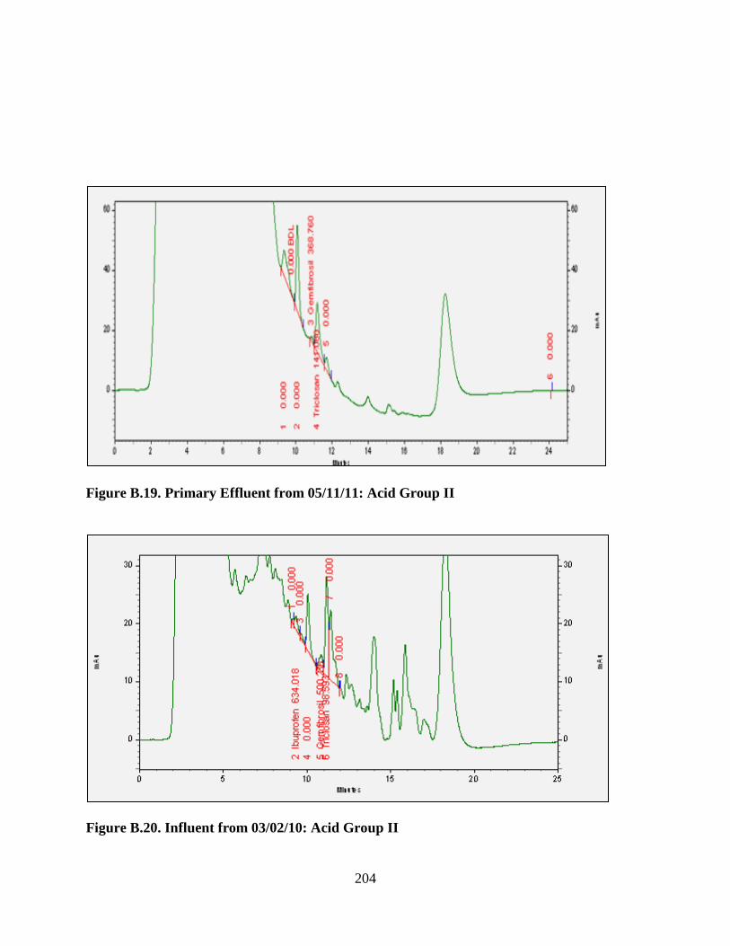
Figure B.19. Primary Effluent from 05/11/11: Acid Group II
Figure B.20. Influent from 03/02/10: Acid Group II
204

Figure B.21. Primary Effluent from 03/02/10: Acidic Group II
Figure B.22. Secondary Effluent from 03/02/10: Acid Group II
205

Figure B.23. Final Effluent from 03/02/10: Acid Group II
Figure B.24. Influent from 06/25/10: Acid Group II
206
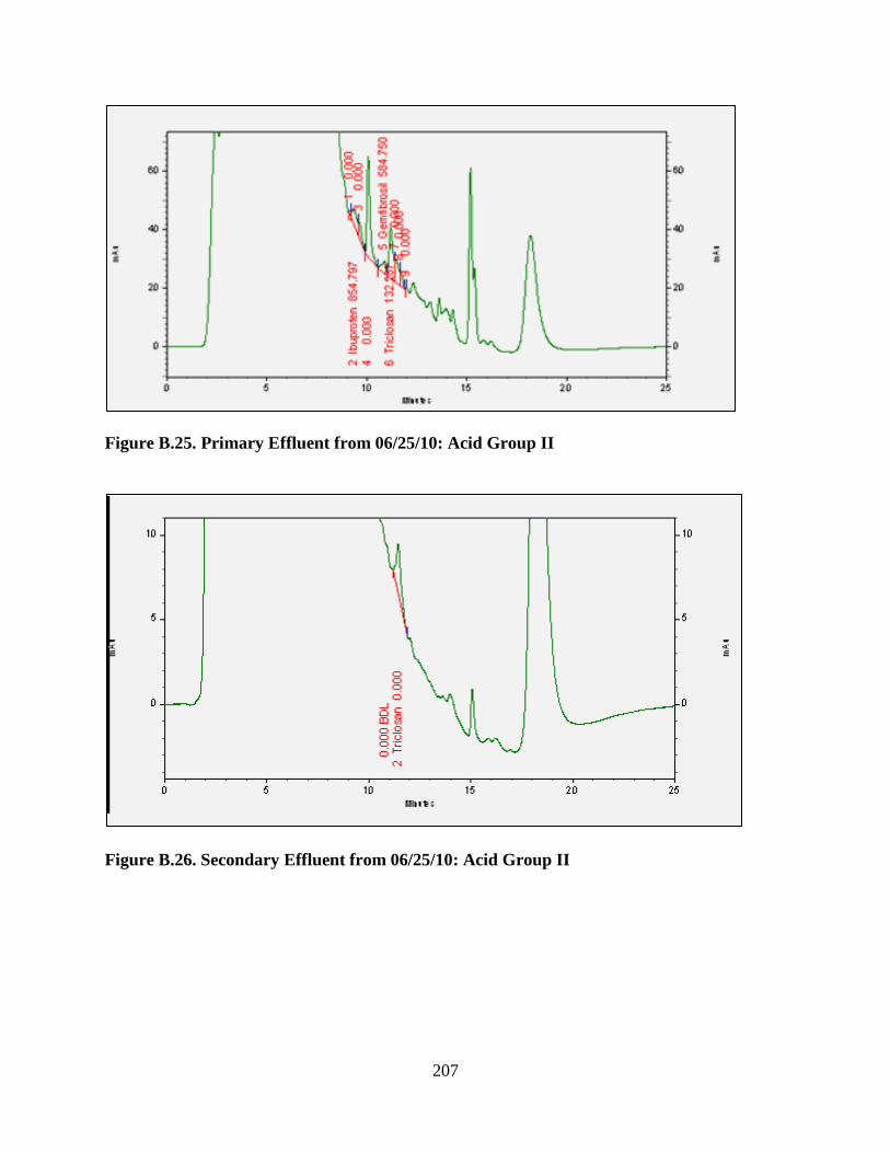
Figure B.25. Primary Effluent from 06/25/10: Acid Group II
Figure B.26. Secondary Effluent from 06/25/10: Acid Group II
207

Figure B.27. Final Effluent from 06/25/10: Acid Group II
Figure B.28. Influent from 11/02/10: Acid Group II
208

Figure B.29. Primary Effluent from 11/02/10: Acid Group II
Figure B.30. Secondary Effluent from 11/02/10: Acid Group II
209
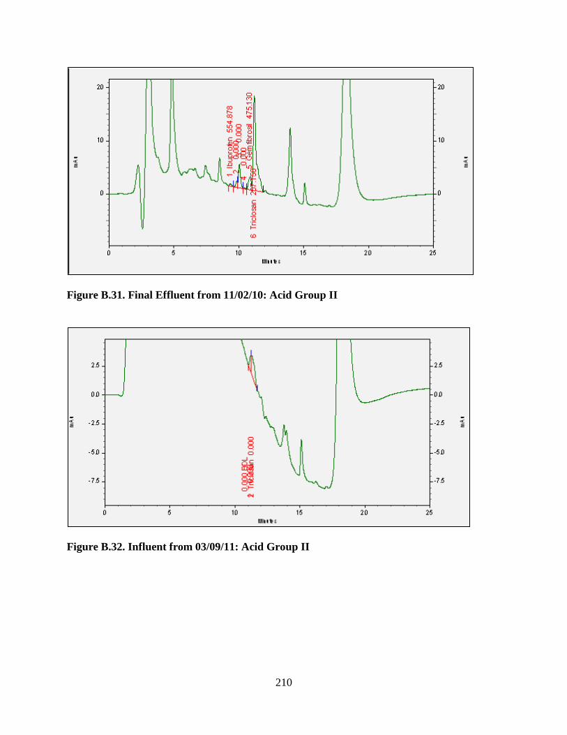
Figure B.31. Final Effluent from 11/02/10: Acid Group II
Figure B.32. Influent from 03/09/11: Acid Group II
210

Figure B.33. Primary Effluent from 03/09/11: Acid Group II
Figure B.34. Secondary Effluent from 03/09/11: Acid Group II
211

Figure B.35. Final Effluent from 03/09/11: Acid Group II
Figure B.36. Influent from 05/14/11: Acid Group II
212

Figure B.37. Primary Effluent from 05/14/11: Acid Group II
Figure B.38. Secondary Effluent from 05/14/11: Acid Group II
213

Figure B.39. Final Effluent from 05/14/11: Acid Group II
Figure B.40. Influent from 09/20/11: Acid Group II
214

Figure B.41. Primary Effluent from 09/20/11: Acid Group II
Figure B.42. Secondary Effluent from 09/20/11: Acid Group II
215
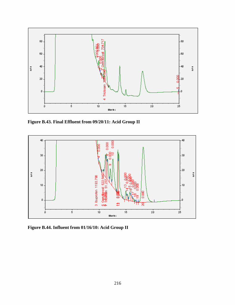
Figure B.43. Final Effluent from 09/20/11: Acid Group II
Figure B.44. Influent from 01/16/10: Acid Group II
216
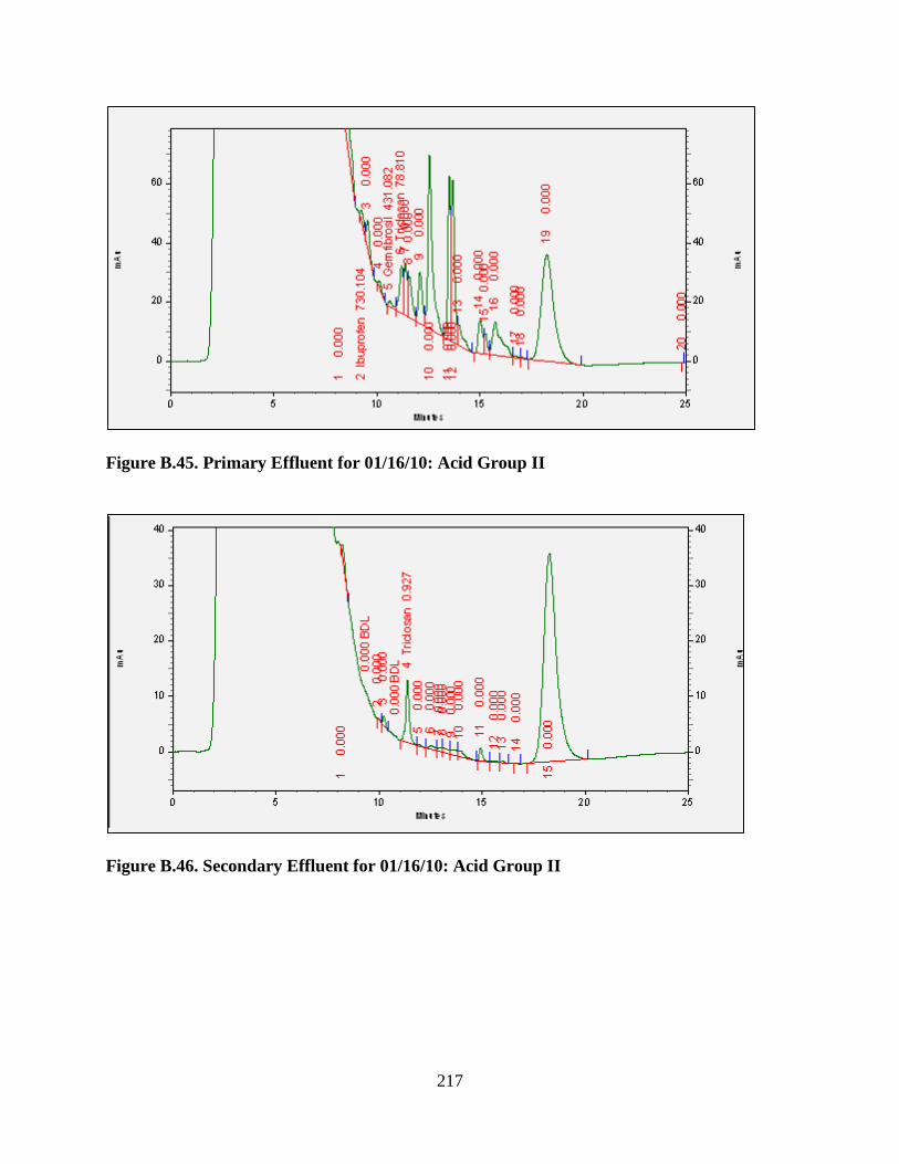
Figure B.45. Primary Effluent for 01/16/10: Acid Group II
Figure B.46. Secondary Effluent for 01/16/10: Acid Group II
217

Figure B.47. Final Effluent for 01/16/10: Acid Group II
Figure B.48. Influent from 03/20/11: Acid Group II
218

Figure B.49. Primary Effluent from 03/20/11: Acid Group II
Figure B.50. Secondary Effluent for 03/20/12: Acid Group II
219

Figure B.51. Final Effluent for 03/20/12: Acid Group II
Figure B.52. Influent from 06/16/12: Acid Group II
220

Figure B.53. Primary Effluent from 06/16/12: Acid Group II
Figure B.54. Secondary Effluent from 06/16/12: Acid Group II
221

Figure B.55. Final Effluent for 06/16/12: Acid Group II
Figure B.56. Influent from 09/15/12: Acid Group II
222

Figure B.57. Primary Effluent from 09/15/12: Acid Group II
Figure B.58. Secondary Effluent from 09/15/12: Acid Group II
223

Figure B.59. Final Effluent from 09/15/12: Acid Group II
Figure B.60. Influent from 11/01/12: Acid Group II
224

Figure B.61. Primary Effluent from 11/01/12: Acid Group II
Figure B.62. Secondary Effluent from 11/01/12: Acid Group II
225

Figure B.63. Final Effluent from 11/01/12: Acid Group II
Figure B.64. Influent from 11/04/12: Acid Group II
226

Figure B.65. Primary Effluent from 11/04/12: Acid Group II
Figure B.66. Secondary Effluent from 11/04/12: Acid Group II
227

Figure B.67. Final Effluent from 11/04/12: Acid Group II
228

APPENDIX C: QUALITY ASSURANCE AND QUALITY CONTROL DATA
Figure C.1. Standard Curve for Naphthalene Y = 26.29821X + 318.6786 R2 = 0.9637912 R = 0.9817287 External Standard Curve: Linear Origin: Force Through(Polyline) Mean RF : 29.49726 RF SD : 14.64758 RF %RSD : 49.65744 0, 20, 40, 60, 80, 100, and 120 ppb were used for calibration
0.0 25.0 50.0 75.0 100.0 Conc.0.0
1.0
2.0
3.0
Area(x1,000)
229
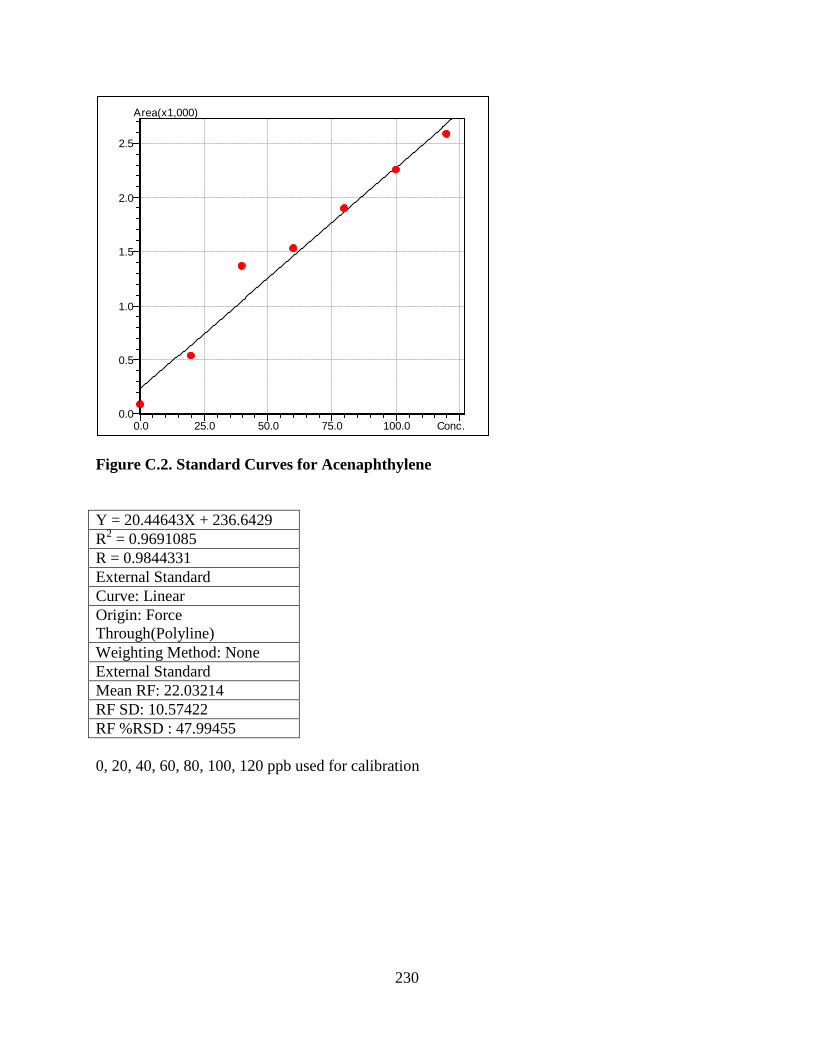
Figure C.2. Standard Curves for Acenaphthylene Y = 20.44643X + 236.6429 R2 = 0.9691085 R = 0.9844331 External Standard Curve: Linear Origin: Force Through(Polyline) Weighting Method: None External Standard Mean RF: 22.03214 RF SD: 10.57422 RF %RSD : 47.99455 0, 20, 40, 60, 80, 100, 120 ppb used for calibration
0.0 25.0 50.0 75.0 100.0 Conc.0.0
0.5
1.0
1.5
2.0
2.5
Area(x1,000)
230
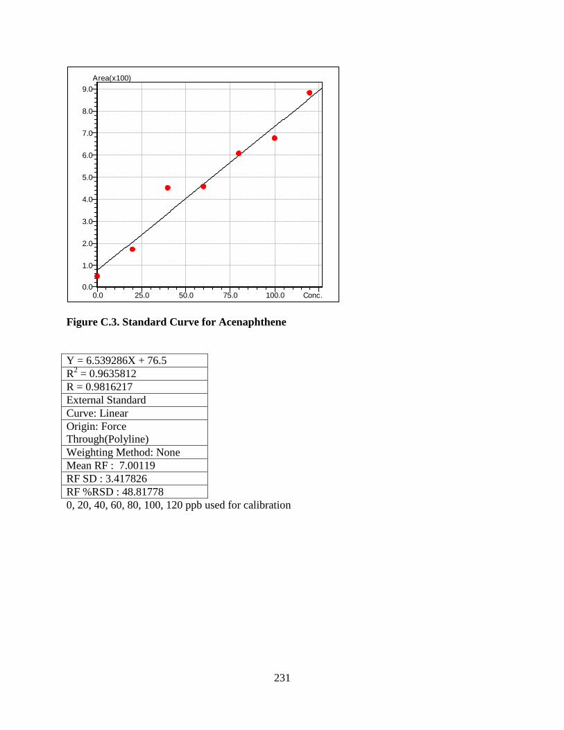
Figure C.3. Standard Curve for Acenaphthene Y = 6.539286X + 76.5 R2 = 0.9635812 R = 0.9816217 External Standard Curve: Linear Origin: Force Through(Polyline) Weighting Method: None Mean RF : 7.00119 RF SD : 3.417826 RF %RSD : 48.81778 0, 20, 40, 60, 80, 100, 120 ppb used for calibration
0.0 25.0 50.0 75.0 100.0 Conc.0.0
1.0
2.0
3.0
4.0
5.0
6.0
7.0
8.0
9.0Area(x100)
231

Figure C.4. Standard Curve for Fluorene Y = 24.46786X + 237.7857 R2 = 0.9584859 R = 0.9790229 External Standard Curve: Linear Origin: Force Through(Polyline) Weighting Method: None Mean RF : 25.56071 RF SD : 12.33030 RF %RSD : 48.23928 0, 20, 40, 60, 80, 100, 120 ppb used for calibration
0.0 25.0 50.0 75.0 100.0 Conc.0.0
0.5
1.0
1.5
2.0
2.5
3.0
Area(x1,000)
232

Figure C.5. Standard Curve for Phenanthrene Y = 23.75179X + 353.6071 R2 = 0.9329065 R = 0.9658708 External Standard Curve: Linear Origin: Force Through(Polyline) Weighting Method: None Mean RF : 27.49845 RF SD : 13.72379 RF %RSD : 49.90752 0, 20, 40, 60, 80, 100, 120 ppb used for calibration
0.0 25.0 50.0 75.0 100.0 Conc.0.0
0.5
1.0
1.5
2.0
2.5
3.0Area(x1,000)
233

Figure C.6. Standard Curve for Anthracene Y = 42.61429X + 351.1429 R2 = 0.9746687 R = 0.9872531 External Standard Curve: Linear Origin: Force Through(Polyline) Weighting Method: None Mean RF : 43.33095 RF SD : 19.96458 RF %RSD : 46.07465 0, 20, 40, 60, 80, 100, 120 ppb used for calibration
0.0 25.0 50.0 75.0 100.0 Conc.0.0
1.0
2.0
3.0
4.0
5.0
Area(x1,000)
234

Figure C.7. Standard Curve for Fluoranthene Y = 27.46786X + 408.9286 R2 = 0.9403727 R = 0.9697282 External Standard Curve: Linear Origin: Force Through(Polyline) Weighting Method: None Mean RF : 30.94845 RF SD : 15.42490 RF %RSD : 49.84064 0, 20, 40, 60, 80, 100, 120 ppb used for calibration
0.0 25.0 50.0 75.0 100.0 Conc.0.0
0.5
1.0
1.5
2.0
2.5
3.0
3.5
Area(x1,000)
235

Figure C.8. Standard Curve for Pyrene Y = 30.62321X + 358.8929 R2 = 0.9465796 R = 0.9729232 External Standard Curve: Linear Origin: Force Through(Polyline) Weighting Method: None Mean RF : 32.51202 RF SD : 16.25551 RF %RSD : 49.99846 0, 20, 40, 60, 80, 100, 120 ppb used for calibration
0.0 25.0 50.0 75.0 100.0 Conc.0.0
0.5
1.0
1.5
2.0
2.5
3.0
3.5
Area(x1,000)
236

Figure C.9. Standard Curve for Chrysene Y = 13.02143X + 171.8571 R2 = 0.9204694 R = 0.959411 External Standard Curve: Linear Origin: Force Through(Polyline) Weighting Method: None Mean RF : 32.51202 RF SD : 16.25551 RF %RSD : 49.99846
0.0 25.0 50.0 75.0 100.0 Conc.0.00
0.25
0.50
0.75
1.00
1.25
1.50
1.75Area(x1,000)
237

Figure C.10. Standard Curve for Ibuprofen
238
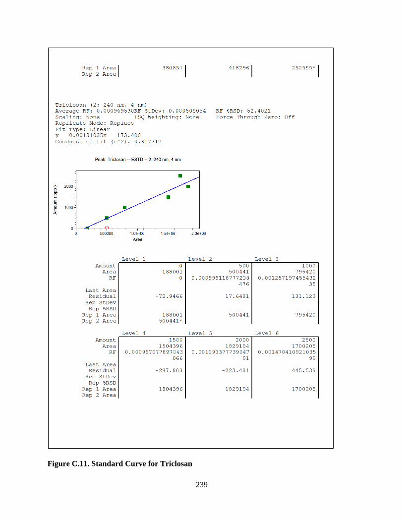
Figure C.11. Standard Curve for Triclosan
239

Figure C.12. Standard Curve for Gemfibrozil
240

Figure C.13. Standard Curve for Sulfamethoxazole
241

Figure C.14. Standard Curve for Carbamazepine
242

Figure C.15. Standard Curve for Fluoxetine
243

Pesticides Surrogate recovery analyses for each sample (acceptable recoveries are 70 to 130%):
IS_1,3-Dimethyl-2- Nitrobenzene (S) IS_Perylene-d12 (S) IS_Triphenylphosphate (S) Pyrene-d10 (S)
Sample flags:
Primary 011610 IS_1,3-Dimethyl-2- Nitrobenzene (S) (244%) 1 Influent 011610 IS_1,3-Dimethyl-2- Nitrobenzene (S) (383%) 3
IS_1,3-Dimethyl-2- Nitrobenzene (S) (249%) (duplicate) 2
Influent 062510 Pyrene-d10 (S) (62.1%) 4 Primary 110210 IS_1,3-Dimethyl-2- Nitrobenzene (S) (215%) 5
Influent 110210 IS_1,3-Dimethyl-2- Nitrobenzene (S) (159%) 6
PARAMETER QUALIFIERS\FLAGS
1) The surrogate IS_1,3-Dimethyl-2-Nitrobenzene for method EPA 525.2 was outside of control limits. The % Recovery was reported as 244 and the control limits were 70 to 130. This result was reported at a dilution of 1.
2) The surrogate IS_1,3-Dimethyl-2-Nitrobenzene for method EPA 525.2 was outside of control limits. The % Recovery was reported as 249 and the control limits were 70 to 130. This result was reported at a dilution of 2.
3) The surrogate IS_1,3-Dimethyl-2-Nitrobenzene for method EPA 525.2 was outside of control limits. The % Recovery was reported as 383 and the control limits were 70 to 130. This result was reported at a dilution of 1.
4) The surrogate Pyrene-d10 for method EPA 525.2 was outside of control limits. The % Recovery was reported as 62.1 and the control limits were 70 to 130. This result was reported at a dilution of 1.
5) The surrogate IS_1,3-Dimethyl-2-Nitrobenzene for method EPA 525.2 was outside of control limits. The % Recovery was reported as 215 and the control limits were 70 to 130. This result was reported at a dilution of 1.
6) The surrogate IS_1,3-Dimethyl-2-Nitrobenzene for method EPA 525.2 was outside of control limits.
244
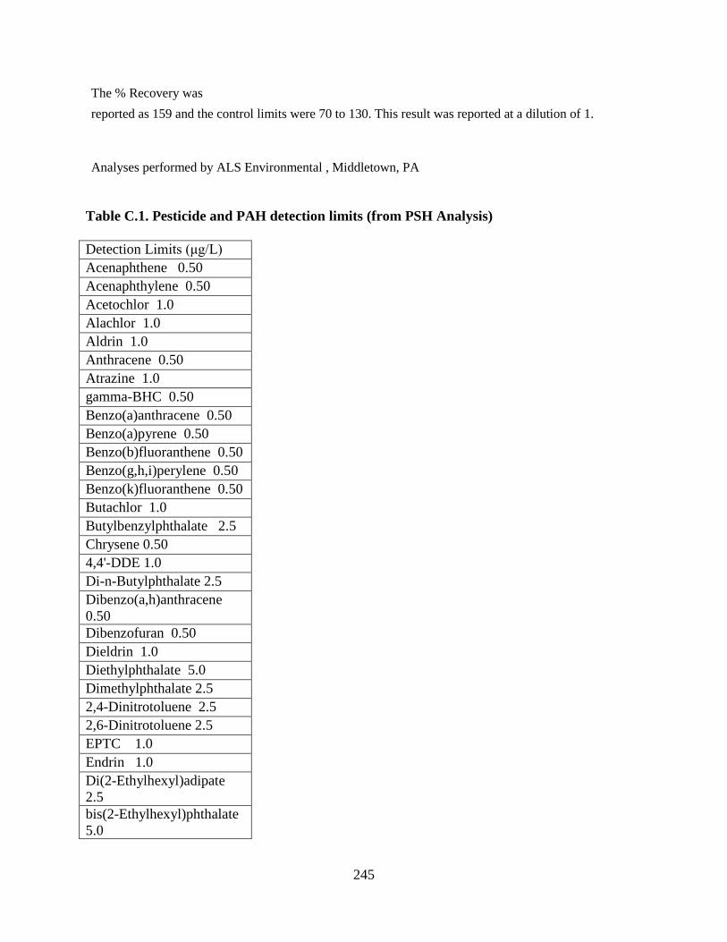
The % Recovery was reported as 159 and the control limits were 70 to 130. This result was reported at a dilution of 1.
Analyses performed by ALS Environmental , Middletown, PA
Table C.1. Pesticide and PAH detection limits (from PSH Analysis) Detection Limits (μg/L) Acenaphthene 0.50 Acenaphthylene 0.50 Acetochlor 1.0 Alachlor 1.0 Aldrin 1.0 Anthracene 0.50 Atrazine 1.0 gamma-BHC 0.50 Benzo(a)anthracene 0.50 Benzo(a)pyrene 0.50 Benzo(b)fluoranthene 0.50 Benzo(g,h,i)perylene 0.50 Benzo(k)fluoranthene 0.50 Butachlor 1.0 Butylbenzylphthalate 2.5 Chrysene 0.50 4,4'-DDE 1.0 Di-n-Butylphthalate 2.5 Dibenzo(a,h)anthracene 0.50 Dibenzofuran 0.50 Dieldrin 1.0 Diethylphthalate 5.0 Dimethylphthalate 2.5 2,4-Dinitrotoluene 2.5 2,6-Dinitrotoluene 2.5 EPTC 1.0 Endrin 1.0 Di(2-Ethylhexyl)adipate 2.5 bis(2-Ethylhexyl)phthalate 5.0
245

Fluoranthene 0.50 Fluorene 0.50 Heptachlor 0.50 Heptachlor Epoxide 0.50 Hexachlorobenzene 0.50 Hexachlorocyclopentadiene 1.0 Indeno(1,2,3-cd)pyrene 0.50 Methoxychlor 1.0 2-Methylnaphthalene 1.0 Metolachlor 1.0 Metribuzin 1.0 Molinate 1.0 Naphthalene 1.0 Phenanthrene 0.50 Propachlor 1.0 Pyrene 0.50 Simazine 1.0 Terbacil 2.5 2,4,5-Trichlorobiphenyl 0.50
246