Embed Size (px)
Citation preview

Tree Reconstruction by Maximum Likelihood
using Prior Knowledge
Bjørn Rohde Jensen
Supervisor: Christian Nørgaard Storm Pedersen
June 23, 2008Department of Computer Science
University of Aarhus
IT-parken, Aabogade 34
8200 Aarhus N.

ii

iii
AbstractIn the field of phylogenetics evolution of species is often described as the
result of random mutations and natural selection, which gives rise to the no-tion of phylogenetic trees. The large amount of high quality sequence dataavailable has made the reconstruction of phylogenetic trees from sequencedata possible. The maximum likelihood method is a powerful and popu-lar choice for constructing phylogenetic trees from sequence data, howeverfinding the maximum likelihood tree is a hard problem requiring numeri-cal methods, limiting the size of the trees, which can be constructed. Thesubject of this thesis is speeding up tree reconstruction by making use ofprior knowledge. We propose a new heuristic for incorporating a phyloge-netic tree in the search for the maximum likelihood tree for similar data set.In this thesis we implement both the proposed heuristic and a simulatedannealing algorithm for finding the maximum likelihood tree from a multi-ple alignment. The experiments performed show, that incorporating priorknowledge leads to a significant speed up, if large amounts are included.The implemented annealing algorithm turned out to be too inefficient totest the heuristic on very large trees.
ResumeEvolution beskrives ofte indenfor fylogenetiken som resultatet af til-
fældige mutationer samt naturlig udvælgelse. Ifølge denne model beskrivesarters udviklings historie ved fylogenetiske træer. Adgangen til betydeligemængder af sekvens information af høj kvalitet har gjort konstruktion affylogenetiske træer udfra sekvens information mulig. Maximum likelihoodmetoden er en populær og kraftig metode til at konstruere fylogenetisketræer fra sekvens information, men at find det optimale træ er et hardt prob-lem, som i praksis kræver numeriske metoder, hvilket igen sætter grænserfor størrelsen af træer, der kan bygges. Malet med dette speciale er at un-dersøge om konstruktionen af fylogenetiske træer kan udføres hurtigere vedat inkludere eksisterende viden. Vi introducerer i specialet en ny heuris-tik til at benytte et eksisterende fylogenetiske træ i søgningen efter detoptimale træ for et lignende data sæt. I specialet har vi implementeretbade den nye heuristik samt en algoritme baseret pa simulated annealingtil at finde det optimale fylogenetiske træ udfra sekvens data i form af etmultiple alignment. De udførte eksperimenter viser, at det er muligt at re-ducere udførselstiden kraftigt, hvis man lader store mængder eksisterendeviden indga i søgningen. Den implementerede annealing algoritme viste sigdesværre ikke i stand til at handtere meget store trær.

iv
Contents
1 Introduction 1
1.1 Structure of the Thesis . . . . . . . . . . . . . . . . . . . . . . 2
2 Phylogenetic Trees 5
2.1 Phylogenetic Trees . . . . . . . . . . . . . . . . . . . . . . . . 5
2.2 Multiple Alignments . . . . . . . . . . . . . . . . . . . . . . . 6
3 Maximum Likelihood 9
3.1 DNA/RNA evolution models . . . . . . . . . . . . . . . . . . 9
3.2 The likelihood of a tree . . . . . . . . . . . . . . . . . . . . . 12
3.3 The pruning Algorithm . . . . . . . . . . . . . . . . . . . . . 14
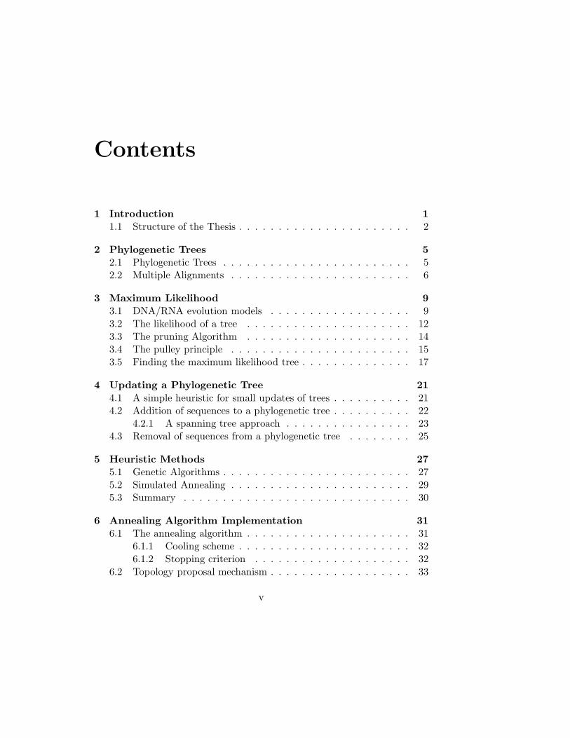
3.4 The pulley principle . . . . . . . . . . . . . . . . . . . . . . . 15
3.5 Finding the maximum likelihood tree . . . . . . . . . . . . . . 17
4 Updating a Phylogenetic Tree 21
4.1 A simple heuristic for small updates of trees . . . . . . . . . . 21
4.2 Addition of sequences to a phylogenetic tree . . . . . . . . . . 22
4.2.1 A spanning tree approach . . . . . . . . . . . . . . . . 23
4.3 Removal of sequences from a phylogenetic tree . . . . . . . . 25
5 Heuristic Methods 27
5.1 Genetic Algorithms . . . . . . . . . . . . . . . . . . . . . . . . 27
5.2 Simulated Annealing . . . . . . . . . . . . . . . . . . . . . . . 29
5.3 Summary . . . . . . . . . . . . . . . . . . . . . . . . . . . . . 30
6 Annealing Algorithm Implementation 31
6.1 The annealing algorithm . . . . . . . . . . . . . . . . . . . . . 31
6.1.1 Cooling scheme . . . . . . . . . . . . . . . . . . . . . . 32
6.1.2 Stopping criterion . . . . . . . . . . . . . . . . . . . . 32
6.2 Topology proposal mechanism . . . . . . . . . . . . . . . . . . 33
v

vi CONTENTS
6.2.1 Model parameter optimization . . . . . . . . . . . . . 336.2.2 Branch length optimization . . . . . . . . . . . . . . . 33
6.3 Topology changing operations . . . . . . . . . . . . . . . . . . 356.3.1 Nearest Neighbor Interchange . . . . . . . . . . . . . . 356.3.2 Subtree Prune and Regrafting . . . . . . . . . . . . . . 366.3.3 Tree bisection and recombination . . . . . . . . . . . . 386.3.4 Discussion . . . . . . . . . . . . . . . . . . . . . . . . . 40
6.4 Optimizations . . . . . . . . . . . . . . . . . . . . . . . . . . . 416.4.1 Subtree equivalence vectors . . . . . . . . . . . . . . . 416.4.2 Partial tree optimization . . . . . . . . . . . . . . . . . 436.4.3 Discussion . . . . . . . . . . . . . . . . . . . . . . . . . 43
6.5 Parallelization . . . . . . . . . . . . . . . . . . . . . . . . . . . 456.5.1 Parallelization of likelihood vector calculation . . . . . 456.5.2 Parallelization of topology exploration . . . . . . . . . 46
6.6 Summary . . . . . . . . . . . . . . . . . . . . . . . . . . . . . 48
7 Tree Update Implementation 49
7.1 Mapping an old multiple alignment to a new . . . . . . . . . 497.2 Distance matrix . . . . . . . . . . . . . . . . . . . . . . . . . . 507.3 Updating the tree . . . . . . . . . . . . . . . . . . . . . . . . . 54
8 Experiments 57
8.1 Tree construction using Neighbor-Joining . . . . . . . . . . . 578.2 Incremental tree construction . . . . . . . . . . . . . . . . . . 58
8.2.1 The size of updates . . . . . . . . . . . . . . . . . . . . 598.2.2 Different sizes of trees . . . . . . . . . . . . . . . . . . 60
8.3 Updating a Phylogenetic Tree . . . . . . . . . . . . . . . . . . 618.4 Parallelization . . . . . . . . . . . . . . . . . . . . . . . . . . . 65
8.4.1 Scaling . . . . . . . . . . . . . . . . . . . . . . . . . . 658.5 Local maxima . . . . . . . . . . . . . . . . . . . . . . . . . . . 68
9 Conclusion 71

Chapter 1
Introduction
Phylogenetic trees have long been used in biology to organize known speciesin families, subfamilies and so forth based on common characteristics deter-mined by direct observation. It is implicit in the organization of species intoa phylogenetic tree, that properties of a species are to some extent sharedwith its neighbors. While this is rather obvious, the implications are quiteprofound. It allows biologists to place a new species in a phylogenetic treebased on easily identified characteristics and in doing so obtain likely an-swers to characteristics not easily identified. Simply put, if it looks like acat, it probably behaves like a cat.
A phylogenetic tree is more than just a classification scheme, it is alsoa history of the evolution of species according to the theory of evolutionintroduced by Darwin; species sharing a great deal of characteristics musthave split recently, while species having few shared characteristics must havesplit long ago. The construction of one big phylogenetic tree, called the treeof life, modeling the evolution of every known species is of great academicinterest in itself and for the insights into the processes of evolution, it brings.
Classification based on direct observations has its limitations; bacteriado not have readily identifiable characteristics, and there are many casesof very distantly related species developing similar characteristics long afterthey split. One such example is color vision, which both primates and birdshave evolved.
The explosion of DNA sequence data over the last decade as illustratedby the graph of the number of base pairs in the Genbank sequence data basein figure 1.1 has spurred interest in the construction of large phylogenetictrees based on sequence data alone. The problem is a hard one in part due tothe large amounts of data but also from a strictly algorithmic view as both
1

2 CHAPTER 1. INTRODUCTION
0
1e+10
2e+10
3e+10
4e+10
5e+10
6e+10
1980 1985 1990 1995 2000 2005
Bas
e P
airs
Year
Figure 1.1: Growth of the Genbank sequence database
maximum parsimony and maximum likelihood, which are the most popularmethods of inferring phylogenetic trees, have been proven NP-hard[5, 4].
A lot of research has been done on the construction of phylogenetic treesfrom sequence data, the majority of the work assume no prior knowledgeabout the tree to be constructed, which in practice is rarely the case. Thefocus of this thesis is to investigate, if it is possible to make use of priorknowledge in the form of known phylogenetic trees for closely related datasets, when inferring phylogenetic trees to arrive at better trees in shortertime.
This work is based primarily on the works of Stamatakis[26, 25] andFelsenstein[8]. The real data sets used were multiple alignments extractedfrom the ARB[16] data base and provided by Niels Larsen from “DanskGenom Institut”, who also helped with insights into the underlying biology.
1.1 Structure of the Thesis
The subject of this thesis is the construction of phylogenetic trees from se-quence data in the form of multiple alignments by means of the maximumlikelihood method. A new heuristic for incorporating knowledge about sim-ilar multiple alignment in the search for the maximum likelihood tree isproposed, implemented and tested. Furthermore a simulated annealing al-gorithm for finding the maximum likelihood tree is implemented.

1.1. STRUCTURE OF THE THESIS 3
In chapter 2 common terms and definitions in the field of phylogeneticsused throughout this thesis are introduced. Chapter 3 gives a brief intro-duction to the maximum likelihood method. In chapter 4 the new heuristicis proposed. Chapter 5 describes the motivation behind implementing asimulated annealing algorithm rather than a genetic algorithm. A detaileddescription of the implemented annealing algorithm is given in chapter 6,and the implementation of the heuristic is described in chapter 7. Bothimplementations are tested in chapter 8. The conclusion of the thesis workis presented in chapter 9.
The implementations and all data sets are available at:
http://www.daimi.au.dk/~u920550/
The implementations are command line programs requiring quite a few pa-rameters, which make direct usage a bit cumbersome. Several sample runscripts can be found in the data directories included in “thesis.tar.bz2”.

4 CHAPTER 1. INTRODUCTION

Chapter 2
Phylogenetic Trees
In this chapter we introduce common terms and definitions in the field ofphylogenetics used throughout this thesis. The terms central to this workare phylogenetic trees and multiple alignments.
2.1 Phylogenetic Trees
A phylogenetic tree is a representation of the evolution of a set of species,where the species are grouped together based on similarity. The species cor-respond to leaves of the tree, and internal nodes correspond to hypotheticalcommon ancestors of these species. The branch lengths of the tree are ameasure of the evolutionary distance between the species, ancestor or not.The topology of a phylogenetic tree refers to the tree’s branching pattern. Itis important to note, that representing evolution by a tree is only a model,there are processes in evolution working outside of a tree like model such asDNA transfers by viruses.
In this context a phylogenetic tree is an unrooted binary tree, which rep-resents the evolution of a set of species represented by a set of DNA or RNAsequences in the form of a multiple alignment. DNA is short for deoxyri-bonucleic acid. It is a class of molecules found in all known living organismsfrom bacteria to humans, where they store genetic information and regulatecell function. DNA molecules are complex double helix structures com-posed of a sugar backbone and the amino acids adenine, thymine, guanineand cytosine, but for the purpose of phylogenetics, only their compositionis considered. The composition of a DNA molecule can be represented by astring over the alphabet A,T,G and C by reading along the backbone fromone end to the other. RNA is short for ribonucleic acid. It is another class
5

6 CHAPTER 2. PHYLOGENETIC TREES
Hum
an
Chi
mpa
nzee
Gor
illa
Figure 2.1: Phylogenetic subtree tree with humans and two closest relatedprimates
of molecules much like DNA with a sugar backbone and four amino acidbases. The RNA considered here is the special class of ribosomal RNA,which comes from the ribosomes also found in all known living organisms,where they are involved in decoding genetic information. The compositionof a RNA molecule can also be represented by a string over an alphabet likeDNA, but in this case the alphabet is A,U,G and C corresponding to theamino acids adenine, uracil, guanine and cytosine.
2.2 Multiple Alignments
Multiple alignment is a generalization of pairwise alignment, which is theproblem of finding the set of insertions, deletions and point mutations withthe highest score transforming one sequence to the other, to more than twosequences. Figure 2.2 is a small excerpt from the multiple alignment forarchaea and eukaryots used here. In order to construct a good phylogenetictree the underlying sequence data needs to be of high quality, but acquir-ing long sequences of high quality data from highly conserved regions of alarge number of species is not an easy task. And multiple alignment is a NP-hard problem[6], requiring heuristic methods in practice[10]. While multiplealignment is an interesting problem with a rich literature and implementedheuristics available, it will not be treated here, and sequence data is sim-

2.2. MULTIPLE ALIGNMENTS 7
-G---A-A-C--A------------UU------------------A-U---A-C--C
-G---U-C-C--A------------C-------------------UAC---G-C--C
-A---C-G-C--A------------U-------------------A-U-UUG-C--U
-A---C-G-C--A------------U-------------------A-U-UUG-C--U
-A---C-G-C--A------------U-------------------A-U-UUG-C--U
-A---C-G-C--A------------U-------------------A-U-UUG-C--U
-C---C-G-C--A------------U-------------------A-U-AUG-C--U
-C---C-G-C--A------------U-------------------A-U-AUG-C--U
-A---C-G-C--A------------U-------------------A-U-AUG-C--U
-C---C-G-C--A------------U-------------------A-U-CUG-C--U
Figure 2.2: Excerpt of the ten first sequences from the multiple alignmentof archaea and eukaryots from the ARB database. The actual sequences arequite long, thus only positions 3604 to 3660 are shown for each sequence.The letters A,U,G and C represent the four bases found in RNA, whilethe dashes represent gaps in the alignment. Gaps are the generalization ofinsertions in pairwise alignment.
ply assumed available as multiple alignments. Multiple alignments come inmany different formats with additional information and annotations, but forthe purpose this thesis, a multiple alignment is simply a set of equal lengthstrings over a particular alphabet. The ARB database[16] contains riboso-mal RNA from regions believed to be the most highly conserved and con-taining significant phylogenetic information, it is as such an obvious choicefor inferring phylogenetic trees.
The number of possible topologies for an unrooted binary phylogenetictree over n species is[3]:
n∏
i=3
(2i − 5), (2.1)
which can easily be shown using the simple observation, that a tree with nleaves can be constructed by inserting an internal node with a single leafinto any one of the edges of a tree with n−1 leaves. An unrooted binary treewith n−1 leaves has 2n−4 nodes and thus 2n−5 edges. The product formsimply corresponds to constructing a random tree by sequential addition.
The rapid growth in the number of possible topologies is at the heart ofproblem surrounding the construction of large phylogenetic trees. Further-more there are 2n − 3 branch lengths to be determined for each topology.

8 CHAPTER 2. PHYLOGENETIC TREES

Chapter 3
Maximum Likelihood
In this chapter we give a brief introduction to the maximum likelihoodmethod The likelihood of a phylogenetic tree is defined, and we cast in-ference of phylogenetic trees in the form of a combinatorial optimizationproblem.
The maximum likelihood method was invented by Fisher[9] and later ap-plied to molecular sequences by Neyman[19], it is now the method of choicefor inferring phylogenies from sequence data. Maximum likelihood hasproven itself superior to distance methods like UPGMA[24] and Neighbor-Joining[23] and the maximum parsimony method by consistently yieldingbetter trees[27], and being a statistical method it is able to handle sequenc-ing errors and ambiguities. The drawback is, that maximum likelihood is afairly complex model, however the advantages of the model far outweigh thecomplexity and as such, maximum likelihood is the only method consideredhere.
3.1 DNA/RNA evolution models
The Maximum Likelihood method rests firmly on the choice of the under-lying model of DNA or RNA evolution, one of the simplest of these modelswas proposed by Jukes and Cantor[12] and describes evolution as a series ofstochastic single letter substitutions. Each event results in the substitutionof a letter by any of the remaining letters with equal rates as illustrated infig 3.1, where the quantity u is the rate of substitution events. The proba-bility of one letter being substituted by an other letter in a given time spancan easily be found by solving an equivalent model, where each letter has anequal probability of being substituted with any letter including the original.
9

10 CHAPTER 3. MAXIMUM LIKELIHOOD
A G
C U
u/3
u/3
u/3
u/3
u/3
u/3
Figure 3.1: The Jukes-Cantor model of DNA evolution. In this model eachamino acid evolves at rate u into any one of the other three amino acidswith equal probability.
Any substitution, where the letter is the same before and after the event,is unobservable and does not correspond to a substitution event in the orig-inal model, as such only 3
4of the events in the modified model correspond
to events in the old model, which means the rate of substitution events inthe new model must be 4
3u for the rates of observable substitutions in the
two models to match. The substitution events in the modified model havethe pleasant property, that the probability of a substitution resulting in aparticular letter does not depend on the initial letter, thus it is not impor-tant how many events took place in an interval, it only matters whether anytook place or not.
One can view the substitution events in an interval as a simple coin-tossing experiment described by a binomial distribution with a probability ofa substitution event in an interval ∆t of 4
3u∆t, however as time is continuous
the number of events or coin tosses tend to infinity as ∆t tends to zero, andthe binomial distribution can be replaced by its limiting case, the Poisondistribution,
Ψ(x) =∑
i≤x
λie−λ
i!, λ > 0 (3.1)
The probability of at least one event occurring is easily found as the com-plement of the probability of no events occurring given by zero order termof the Poison distribution with λ = 4
3ut,
P (t) = 1 − e−4
3ut. (3.2)

3.1. DNA/RNA EVOLUTION MODELS 11
The probability Pij of a letter being substituted after time t is;
Pij(t) =1
4(1 − e−
4
3ut), i 6= j (3.3)
Pii(t) =1
4(1 + 3e−
4
3ut) (3.4)
where i and j are letters in the alphabet {A,G,C,U/T}.The Jukes-Cantor model can be seen as a special case of a much more
general model called the General Time-Reversible model. Dealing with in-dividual letters becomes somewhat tedious in the general case. It is simplerto work with state vectors representing the probability of observing a letterat a certain site in a sequence, and operators working on these state vectors.The evolution of a state vector x(t) can be described by the propagatorP (t′, t), also known as the evolution operator.
x(t′) = P(t′, t)x(t) (3.5)
The propagator has to obey the composition rule,
P(t′′, t′)P(t′, t) = P(t′′, t), t′′ > t′ > t (3.6)
since time is contiguous, and P obviously has to satisfy,
P(t, t) = I (3.7)
Assuming evolution at different sites in a sequence independent and the tran-sition rates between letters independent of time, then the evolution operatormust satisfy the differential equation,
∂
∂tP(t, t0)x(t0) = AP(t, t0)x(t0), (3.8)
where A is an operator yielding the change in a state vector corresponding toan expected rate of one event per unit of time. Conservation of probabilityrequires
∑
i Aij = 0. The solution is simply;
P(t) = eAt, (3.9)
which, depending on A, may or may not have an analytical form.DNA/RNA evolution models used with likelihood methods are often
limited to time-reversible models for efficiency reasons within these methods.A model is time-reversible, if the evolution operator P for all i, j and t satisfy,
πiPji(t) = πjPij(t), (3.10)

12 CHAPTER 3. MAXIMUM LIKELIHOOD
where πi and πj are the equilibrium probabilities of the letters i and j.
The rate operator A for the General Time-Reversible model with theletters {A,G,C,T} as basis was cast in the following form by Lanave etal [14],
A =
−a απA βπA γπA
απG −b δπG ǫπG
βπC δπC −c ηπC
γπT ǫπT ηπT −d
, (3.11)
where
a = απG + βπC + γπT , (3.12)
b = απA + δπC + ǫπT ,
c = βπA + δπG + ηπT ,
d = γπA + ǫπG + ηπC ,
with the constraint,
1 = 2(πAπGα + πAπCβ + πAπT γ + πGπCδ + πGπT ǫ + πCπT η), (3.13)
to ensure the expected rate of substitution events is one per unit of time.
Comparing the General Time-Reversible model and Jukes-Cantor modelthe difference is stark. Though both are time-reversible, the Jukes-Cantormodel offers very little in terms adaptability to a specific data set, but hassimple analytic forms. The Jukes-Cantor model has in particular been criti-cized for yielding equal equilibrium probabilities for letters in the alphabet,something which is contradicted by experimental data. The General Time-Reversible model is a very flexible model but depends on numerical methods,making it a substantially more demanding task.
3.2 The likelihood of a tree
Consider the joint probability P (T,D) of an evolution hypothesis T and thealignment data D. The law of conditional probability allows P (T,D) to bedecomposed in two ways;
P (T |D)P (D) = P (T,D) = P (D|T )P (T ), (3.14)
where P (T |D) is the probability of the hypothesis T given the data D,and P (D|T ) vice versa. The ratio between the joint probabilities of two

3.2. THE LIKELIHOOD OF A TREE 13
X
Y Z
S4S3S2S1
t1 t2 t3 t4
t5 t6
Figure 3.2: Sample likelihood calculation for a single site. S1 to S4 rep-resent letters in sequences in a multiple alignment, while X,Y and Z areintermediate results. t1 to t6 represent branch lengths.
hypotheses and a single data set can thus be written,
P (T1,D)
P (T2,D)=
P (T1|D)
P (T2|D)=
P (D|T1)P (T1)
P (D|T2)P (T2). (3.15)
The conditional probabilities P (D|T1) and P (D|T2) are called the likelihoodsof T1 and T2 respectively. Assuming the probability of observing letters atdifferent sites are independent, then the conditional probability P (D|T ) canbe written as the product of conditional probabilities P (Di|T ) for each site.
P (T1|D)
P (T2|D)=
(
n∏
i=1
P (Di|T1)
P (Di|T2)
)
P (T1)
P (T2). (3.16)
The ratio between the prior probabilities P (T1) and P (T2) is largely un-known due to the inherent difficulty in determining the prior probabilityof a hypothesis T , however, if the available data contains a large numberof sites and is of sufficient quality to discriminate between given hypothe-ses, the ratio of prior probabilities would be expected to be dominated bythe likelihood ratio, since the data would be expected to consistently favorone hypothesis across all sites. The hypothesis with the maximum likeli-hood is an estimate of the hypothesis with the maximum probability, andit was shown by Fisher[9], that maximum likelihood estimates converge tothe correct value as data, which in this context means the length of multiplealignments, increases.
The likelihood at a single site P (Di|T ) is the sum of the likelihoodsof all possible paths by which letters could have evolved into the observed

14 CHAPTER 3. MAXIMUM LIKELIHOOD
letters. Figure 3.2 illustrates the calculation of the likelihood for a small tree.The evolution along different branches also known as lineages are assumedindependent, thus the probability of for example X evolving into Y and Zis simply the product of the individual probabilities as determined by thechosen model of evolution of the alphabet in question. The likelihood in thiscase is given by;
∑
X
∑
Y
∑
Z
P (X)P (Y |X, t5)P (Z|X, t6)P (S1|Y, t1)P (S2|Y, t2)
P (S3|Z, t3)P (S4|Z, t4), (3.17)
where P (X) is the equilibrium probability of letter X under the chosenmodel of evolution. It is worth noting, that alignments in general containgaps(see figure 2.2), and sequences can contain ambiguities for example dueto limitations of sequencing techniques. Ambiguous data supports severalpaths by weighing the paths with the conditional probabilities of the lettersat the leaves of the tree being interpreted by the sequencing method asthe letters observed at a particular site. The probabilities of observingvarious letters at a given site need not add up to 1, since they correspond toindependent observations. Gaps in sequences are conceptually quite differentfrom sequencing errors but are treated in much the same way. A gap containsno information about the evolution at a particular site and thus supports anyhypothesis fully. Both ambiguities and gaps are easily handled by furthersummation over S1, S2, S3 and S4 and multiplication of the probability ofeach observed letter P (S1)P (S2)P (S3)P (S4). Each factor in this sum iseasily calculated, but the number of terms in general grows exponentiallywith the number of leaves in the tree making the method impractical.
3.3 The pruning Algorithm
Felsenstein introduced a more efficient algorithm than simple summationover terms called the pruning algorithm[7] for calculating the likelihood ofa tree. The algorithm exploits the fact, that, while one must sum over theentire alphabet for each node in the tree, a lot of extra work is performedcalculating the same quantities repeatedly. This is easily seen using the treein figure 3.2 as example by moving the summations in equation 3.17 as farto the right as possible.
∑
X
P (X)[∑
Y
P (Y |X, t5)P (S1|Y, t1)P (S2|Y, t2)] (3.18)
[∑
Z
P (Z|X, t6)P (S3|Z, t3)P (S4|Z, t4)].
3.4. THE PULLEY PRINCIPLE 15
The strong correlation between the topology of a tree and the expressionfor the corresponding likelihood is apparent. The sum over the letters ofa particular internal node only depends on the subtree rooted at the node.This fact suggests, the expression can be evaluated in a bottom up fashionusing dynamic programming, which is exactly what the pruning algorithmdoes.
Central for the algorithm is a quantity known as the conditional likeli-hood of a subtree Li
j(X), where i is the site in the sequence, j is the nodein the tree and X is the letter on which the likelihood of the subtree is con-ditional. The conditional likelihood of the tree rooted at an internal node isgiven by,
Lij(X) = [
∑
sl
P (sl|X, tl)Lil(sl)][
∑
sr
P (sr|X, tr)Lir(sr)], (3.19)
and the conditional likelihood of the subtree corresponding to a leaf is simplythe conditional probability of the letter X resulting in the letter observedat site i in the matching sequence. The pruning algorithm terminates aftercalculating Li
R(X) for the root node, from which the likelihood of the treeis given by,
Li =∑
X
P (X)LiR(X), (3.20)
where P (X) is the equilibrium probability of the letter as before.For an alignment consisting of n sequences of length l over an alphabet
of size z the pruning algorithm runs in time proportional to (n− 1)lz2 as itcalculates (n− 1) subtrees, each effectively requiring two matrix multiplica-tions by evolution matrices, for l sites. The running time of course dependson the choice of evolution model for the alphabet.
3.4 The pulley principle
The likelihood has been defined for rooted trees so far, giving the impression,that the likelihood is only well defined for rooted phylogenetic trees, whiletrue for the most general models, it is not so for the important class oftime reversible evolution models. Recall that a time reversible model forthe evolution of the letters in the alphabet satisfy,
P (y|x, t)πx = P (x|y, t)πy , (3.21)
for any pair of letters x,y and time t. The quantities πx and πy are the equi-librium probabilities of the letters x and y for the chosen model. Consider

16 CHAPTER 3. MAXIMUM LIKELIHOOD
R
t
T1
0
T2
R
t0
T2
T1
Figure 3.3: The Pulley Principle allows the root to be moved along an edgewithout changing the likelihood of tree. The root of the trees consideredhere will always have a child edge of length zero, but the principle does notrequire this. T1 and T2 are general subtrees, and t is the length of the edge,the root is moved through.
the two trees in figure 3.3, where T1 and T2 represent subtrees, which havebeen fully evaluated by means of the pruning algorithm. The likelihood ofthe tree on the left hand side is,
L =∑
R
∑
T1
∑
T2
πRP (T1|R, 0)L1(T1)P (T2|R, t)L2(T2) (3.22)
=∑
T1
∑
T2
πT1L1(T1)P (T2|T1, t)L2(T2). (3.23)
Using time reversibility this becomes,
L =∑
T1
∑
T2
πT2L1(T1)P (T1|T2, t)L2(T2) (3.24)
=∑
R
∑
T1
∑
T2
πRP (T1|R, t)L1(T1)P (T2|R, 0)L2(T2), (3.25)
which is exactly the likelihood of the tree on the right hand side. It can beshown, that the root R can be placed at any point along the line from T1
to T2 and still lead to the same likelihood, but the less general result shownhere will suffice. Consider now the likelihood of the trees in figure 3.4. T1,T2 and T3 are as before arbitrary trees fully evaluated using the pruningalgorithm. The likelihood of the tree on the left hand side is given by,
L =∑
R
∑
Y
∑
T1
∑
T2
∑
T3
πRP (T1|R, t1)L1(T1) (3.26)
3.5. FINDING THE MAXIMUM LIKELIHOOD TREE 17
R
t3
0
t2t1
Y
T2T3
T1
R
t1
t2
0
Yt3
T1T3T2
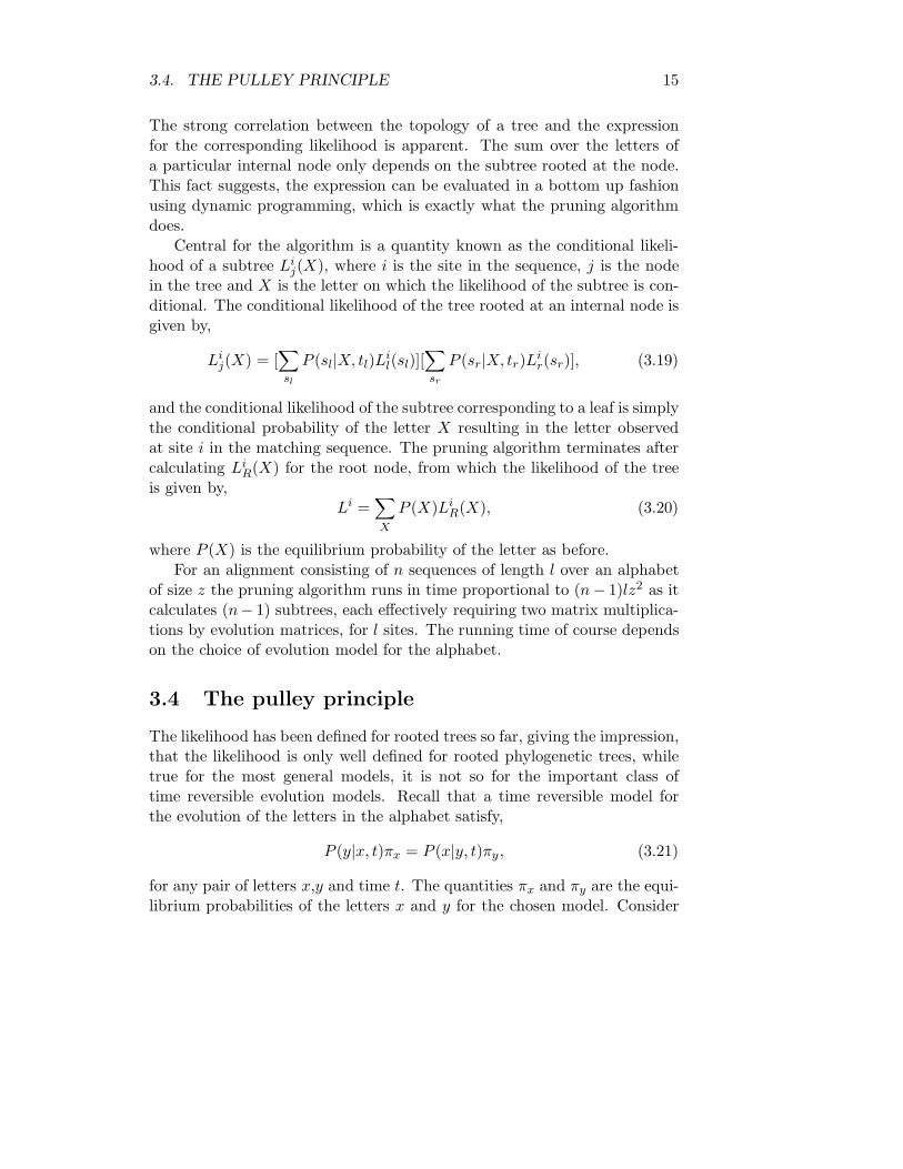
Figure 3.4: The Pulley Principle also allows the root to be moved through anode without changing the likelihood of the tree. T1,T2 and T3 are generalsubtrees, t1 through t3 are edge lengths, and Y is the node, which the rootis moved through.
P (Y |R, 0)P (T2|Y, t2)L2(T2)P (T3|Y, t3)L3(T3)
=∑
R
∑
T1
∑
T2
∑
T3
πRP (T1|R, t1)L1(T1) (3.27)
P (T2|R, t2)L2(T2)P (T3|R, t3)L3(T3)
=∑
R
∑
Y
∑
T1
∑
T2
∑
T3
πRP (Y |R, 0) (3.28)
P (T1|Y, t1)L1(T1)P (T2|Y, t2)L2(T2)P (T3|R, t3)L3(T3),
(3.29)
which is exactly the likelihood of the tree on the right hand side. The pulleyprinciple simply states, the likelihood of a phylogenetic tree does not dependon, how the tree is rooted, if the evolution model is time reversible.
3.5 Finding the maximum likelihood tree
Finding the unrooted binary tree with the maximum likelihood is in principlea simple optimization problem, however the sheer size of the search spacecomplicates matters. Finding the maximum likelihood tree has long beenbelieved to be an NP-hard problem by the community, in no small partdue to its close relationship to its competitor maximum parsimony, whichis similar yet simpler and for decades known to be NP-hard[5], but alsofrom the simple fact, that the search space is exponential in the size of thenumber of sequences. Choir et al [4] recently showed maximum likelihood

18 CHAPTER 3. MAXIMUM LIKELIHOOD
to be NP-complete by reduction from vertex cover.There is no analytical form for determining the optimal branch lengths
of a given topology, but the pruning algorithm and the pulley principle makethe use of numerical methods a viable approach by reducing the number oflikelihood vectors to be recomputed in the face of localized changes to trees.To optimize a single branch, it is necessary to temporarily insert a virtualroot. Suppose a virtual root has to be inserted in an unrooted tree consistingof the subtrees T1 and T2 to optimize the connecting edge of length t, thiscan be done simply by connecting T1 to the virtual root R with an edge oflength zero and connecting T2 to the virtual root R with an edge of lengtht as in figure 3.3. Finding the optimum branch length is then simply aquestion of optimizing the likelihood function given by equation 3.27 with tas the only parameter, assuming the conditional likelihoods of the subtreesare known. In general, the pulley principle makes it possible to place thevirtual root the most favorable place in the tree without any effect on theresult.
Optimizing the branches of the entire tree obviously results in the vir-tual root being moved around a great deal in the tree, which can be doneeasily enough, but the subsequent calculation of the likelihood requires theconditional likelihoods of the subtrees on either side of the branch to beknown. These quantities are easily calculated using the pruning algorithm,but to run the algorithm over the entire tree, every time the root is moved,is to do more work than need be.
For example consider an unrooted tree consisting of three subtrees T1,T2 and T3 connected to an internal node Y by edges t1, t2 and t3 respec-tively. Suppose one wants to move a virtual root from the branch t1 to t3,this corresponds exactly to moving the virtual root through the node Y asillustrated in figure 3.4. Application of the pruning algorithm to the treebefore and after moving the virtual root shows, that the calculations differonly for a single conditional likelihood near the virtual root. If one main-tains the invariant, that all conditional likelihoods for the current rootingare known. It is then easy to see, that one only needs to recalculate theconditional likelihood for the new subtree Y in the new virtual rooting toreestablish the invariant after moving the root.
Thus moving the virtual root during the optimization of the branches ofa tree requires the recalculation of one conditional likelihood for each node,the root is moved through in the process. The cost on the other hand ishaving to store the conditional likelihoods for every node in the tree. Itis important to note, that this mainly benefits topology and branch lengthoptimization, since changes in model parameters have a global impact on

3.5. FINDING THE MAXIMUM LIKELIHOOD TREE 19
the tree and thus invalidate all previous conditional likelihood vectors.

20 CHAPTER 3. MAXIMUM LIKELIHOOD
Chapter 4
Updating a PhylogeneticTree
In this chapter we propose a new heuristic for constructing phylogenetictrees by incorporating prior knowledge in the form of other phylogenetictrees. The heuristic is based on the assumption, that tree topology is to alarge degree conserved through moderate changes to the underlying multiplealignment.
Finding a maximum likelihood tree based only on a multiple alignmentis a very clean way, but it is perhaps also a somewhat wasteful way, sincea great deal is often known about the maximum likelihood tree based onwork on other multiple alignments with significant overlap. One example ofthis is the tree of life, which steadily grows as sequences are added to thedatabases. It is not unreasonable to expect the addition of a small set ofnew sequences to have a minor impact on the overall structure of the tree,and thus to find the structure of the old tree largely conserved within thenew tree.
4.1 A simple heuristic for small updates of trees
If one assumes, similarity between multiple alignments imply similarity be-tween the trees derived from said alignments, one implicitly assumes, thattree topologies are determined by short range effects primarily. This mightnot be the case in maximum likelihood calculations, where several topologyproposals might well have very different topologies while having similar like-lihoods. The addition or removal of a sequence strongly supporting one ormore of these topologies might tip the balance in favor of a very different
21

22 CHAPTER 4. UPDATING A PHYLOGENETIC TREE
A B
T
d
A B
T
ba
t
Figure 4.1: Addition of a sequence to a phylogenetic tree. The edge connect-ing the leaf A and subtree T is removed. The leaves A, B and subtree T areconnected to a new node, the lengths of the connecting edges must ensurethe path length between A and any node in T remains the same, while thelength of the path between A and B corresponds to their similarity.
topology. While such a scenario is obviously possible within the maximumlikelihood model, it would be an indication of a problem with the underly-ing multiple alignment or model parameters, as multiple maxima in practicerarely give rise to problems[8]. It is in other words not unreasonable to ex-pect a tree resulting from updates on an optimal tree for a closely relateddata set to lie in the neighborhood of an optimal tree for the new data set.Furthermore, if the updates are minor, and the phylogenetic signal strong,then the error in neglecting long range effects should be small.
4.2 Addition of sequences to a phylogenetic tree
The addition of a sequence is complicated by the large number of possibleinsertion points in a large tree, however one would expect similar sequencesto be grouped together in a tree, where similarity in this case is expressed interms of evolutionary distance between a pair of sequences according to theunderlying evolution model. One could have based the measure of similarityon the evolutionary distance between likelihood vectors corresponding to anynode in the tree rather than just vectors, which correspond to leaves, butdoing so complicated matters, as the likelihood vectors of leaves depend onlyon the corresponding sequence, while likelihood vectors of internal nodesdepend on topology of the tree, and thus subject to change with everyupdate of the tree.
Figure 4.1 shows the addition of sequence B as a new neighbor to A. Thedesire to leave path lengths between leaves in the original tree unchanged

4.2. ADDITION OF SEQUENCES TO A PHYLOGENETIC TREE 23
requires, a + t = d, and consistency demands a and b sum to the similarityscore between the sequences. This still leaves a free, but a reasonable initialchoice is to strive towards keeping the branch lengths a,b and t of similarsize by setting a equal to b or t whichever is the smaller.
The actual choice of where to add new sequences to the tree is com-plicated by the fact, that different orders of insertion using the describedheuristic give rise to different trees, but since similar sequences are expectedto be grouped together, inserting a sequences as a neighbor to the sequencein the tree, with which it has the highest similarity, is an obvious althoughnot perfect choice. This suggests a greedy algorithm, where the tree isgrown by adding the sequence with the highest similarity, and thus shortestdistance, to a sequence already in the tree. Problems can arise, if thereare what one might call outlier sequences; sequences with low similarity toany sequence in the tree. Such sequences will be added to the least remoteneighbor with a long edge, rather than as a single off shoot from a trunkdeeper in the tree.
4.2.1 A spanning tree approach
Slowly growing a phylogenetic tree by adding sequence upon sequence, al-ways choosing the sequence with the highest similarity to a sequence alreadyin the tree bears a strong resemblance to the Prim-Jarnık algorithm[21] forconstruction of a minimum spanning tree.
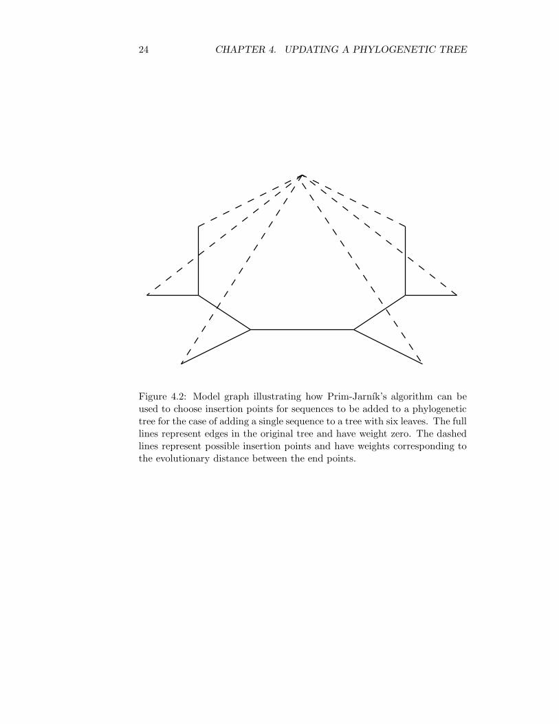
Consider the weighted graph consisting of all the nodes and edges of theold phylogenetic tree, a node for each sequence to be added and edges be-tween all pairs of nodes to be added and edges between all pairs consistingof a node to be added and a node corresponding to a leaf in the originalphylogenetic tree. Furthermore let all edges between nodes correspondingto nodes in the phylogenetic tree have weight zero, and the remaining edgeshave the weight of the similarity between the sequences, the nodes corre-spond to. Executing Prim-Jarnık’s algorithm on this graph starting from anode corresponding to a node in the original phylogenetic tree, until all edgesof weight zero have been added, constructs a tree identical to the originalphylogenetic tree by design. The criterion for selecting edges with a weightgreater than zero to be part of the spanning tree for this graph correspondsexactly to the criterion of the heuristic for adding sequences to the originalphylogenetic tree, but unlike the case of spanning tree construction, recordmust be kept of which nodes have already been added to the phylogenetictree, as the roles of the nodes the chosen edge is incident on are asymmetricin the insertion step. The simplest way to keep track of nodes already in the
24 CHAPTER 4. UPDATING A PHYLOGENETIC TREE
Figure 4.2: Model graph illustrating how Prim-Jarnık’s algorithm can beused to choose insertion points for sequences to be added to a phylogenetictree for the case of adding a single sequence to a tree with six leaves. The fulllines represent edges in the original tree and have weight zero. The dashedlines represent possible insertion points and have weights corresponding tothe evolutionary distance between the end points.

4.3. REMOVAL OF SEQUENCES FROM A PHYLOGENETIC TREE25
B
b
B
TT
S
s
t
S
s+t
Figure 4.3: Removal of a sequence from a phylogenetic tree. The leaf Bcorresponding to the removed sequence is pruned from the tree along withit parent node. subtrees S and T are connected by an edge of length s + tto ensure, the length of the path between any two remaining nodes remainsunaffected.
tree is to mark the nodes, as they are added to the tree. Adding sequences tothe original tree as the corresponding edges in the derived graph are chosenconstructs the new phylogenetic tree in time O(n ∗ (m−n)log(m)), where nis the number of sequences to be added, and m is the number of sequencesin the new phylogenetic tree, requiring only the original phylogenetic treeand a partial distance matrix.
4.3 Removal of sequences from a phylogenetic tree
The removal of a sequence from a phylogenetic is straight forward, it issimply a matter of pruning a leaf from the tree. The process is depictedin figure 4.3, where the leaf B corresponding to the removed sequence andthe connecting internal node are removed and the remaining subtrees S andT connected. The length of this connecting edge has to be determined bynumerical methods, but setting it to s + t leaves the length of the pathbetween any two remaining nodes in the new tree unchanged and should atleast serve as a good initial guess for further refinement.

26 CHAPTER 4. UPDATING A PHYLOGENETIC TREE
Chapter 5
Heuristic Methods
In this chapter we compare the published results by Stamatakis using simu-lated annealing on one hand and on the other hand Lewis and Brauer usinggenetic algorithms to determine, whether simulated annealing or a geneticalgorithm would be better suited to form the basis for implementation withthe purpose of testing the proposed heuristic.
Finding an optimal tree topology in the space of possible topologies ismuch harder than simply optimizing branch lengths, and many different op-timization schemes have been applied. The most obvious approach wouldbe to employ a simple local search heuristic, however the problem is com-pounded by the existence of local optima, which local search heuristics are illequipped to cope with, thus alternatives such as genetic algorithms and sim-ulated annealing have been the focus of much attention in the field. Bothapproaches make use of local topology change moves to explore the treespace, many of which applicable to both.
5.1 Genetic Algorithms
Genetic algorithms mimic the natural evolution process by encoding proper-ties in the genes of a population and then allowing the population to evolveby mutations of individual and combination usually of pairs of solutions toproduce new members of the population. The size of the population is lim-ited by the application of a domain specific fitness function to determine, ifeach individual in the population is sufficiently fit to survive into the nextgeneration. The use of genetic algorithms in optimization is mainly due toHolland[11], and first employed on phylogenies by Matsuda[17].
When applied to Maximum Likelihood the genes of the population usu-
27

28 CHAPTER 5. HEURISTIC METHODS
122
3
9
6
8
7
10
5
4
11
1
1
2
34
5
67
8
9
10
11
128
210116129
1
475
3
ChildParrent 2Parrent 1
Figure 5.1: Recombination move used by Lewis et al. The dotted lineshighlight the subtree selected from the first parent, the leaves pruned fromthe second parent and the subtree in the child,
ally encode the possible tree topologies, the branch lengths are treated byother means. The fitness function is usually simply the likelihood of theindividual. Lewis [15] and Brauer et al [2] report good results with theirGAML genetic algorithm, and efficient use of processing power in parallelversions. In GAML tree topologies are represented as text strings in Newickformat, mutations take the form of random subtree Prune and Regraft oper-ations (figure 6.2) and combinations are carried out by a somewhat elaborateprocedure, where a subtree is chosen from one parent and combined with atree formed by pruning the members of the chosen subtree from the secondparent (figure 5.1). While their results are encouraging, they indicate someproblems, the biggest being large memory and processing power require-ments.
Genetic algorithms while deceptively simple in appearance require care-ful encoding of the parameters of the solution space and choice of pairingscheme for generating offspring, the reported problems with loss of popula-tion diversity and a curiously small effect of changes in the rate of recom-binations suggest problems with the encoding and pairing schemes chosen.The exploration of the tree space by means of mutations and subsequent se-lection appears to work very well on the other hand. Newer results suggest,a great deal of progress has been made in overcoming these short comings.

5.2. SIMULATED ANNEALING 29
The initial population used in genetic algorithms are usually randomgenerated and must be sufficiently large to allow a proper sampling of thesolution space, however it is possible to make use of prior knowledge aboutsolutions and in a sense seed regions of the search space expected to containpossible solutions more densely, however doing so must be done with care,as it reduces the genetic diversity of the population.
The algorithm employed by Lewis et al is fairly complicated, requiresa lot of memory and fine tuning. Furthermore the algorithm appears tohave problems loosing genetic diversity too fast, and attempting to speedconvergence by seeding the initial population with topologies derived byadding or removing leaves from a similar phylogenetic tree seems almostguarantied to exacerbate the problem.
5.2 Simulated Annealing
Simulated annealing was invented by Kirkpatrick et al [13] as a generalizationof Metropolis Monte Carlo simulations of many body systems in physics tooptimization of combinatorial problems. The inspiration for the methodwas the observation, that crystalline materials such as metals manage toarrange themselves in a minimum energy state if cooled sufficiently slowfrom an initial high temperature state.
In Monte Carlo simulations the temperature is usually kept constant dur-ing the simulation, while a property of the system is sampled; Kirkpatrick etal showed how to optimize combinatorial problems by addition of a cool-ing schedule and by generalizing energy and temperature to an arbitraryobjective function defined over a given configuration space. The simulatedannealing algorithm consists of; a method for proposing new configurationsgiven an old, a cooling schedule, the Metropolis-step based on the objectivefunction to be minimized and a stopping criterion.
It can be shown, that simulated annealing will terminate with an optimalconfiguration with a probability tending to 1, as the length of the simula-tion tends towards infinity for an arbitrary initial configuration, providedthe configuration proposal mechanism can generate the entire configurationspace, the initial temperature is sufficiently high to allow all moves and thecooling process is sufficiently slow. Kirkpatrick quickly realized, the processof slow cooling from a high temperature would be impractical due to thelength of such annealing runs and introduced the notion of low temperaturestarts or cold starts. The idea behind low temperature starts is to find agood initial configuration by other means and continue the annealing pro-

30 CHAPTER 5. HEURISTIC METHODS
cess from there starting from a much lower temperature. Exactly how lowthe starting temperature depends on the quality of the initial configuration,with too low a starting temperature or rapid cooling the annealing processis likely to get stuck in local minima.
In practice the performance of a simulated annealing algorithm dependson good choices of configuration proposal mechanism and cooling scheduleto reach an acceptable solution quickly. Stamatakis et al [27] report good re-sults using a simulated annealing approach, where branch length and modelparameter optimization is handled by strict hill climbing, and only opti-mization of the tree topology is performed by actual simulated annealing.Stamatakis et al use subtree prune and regraft(SPR) moves in their topol-ogy proposal mechanism, however they restrict the possible graft points toa neighborhood centered on the prune point. The neighborhood is fully ex-plored using a fast scoring algorithm, the best candidate is then subjectedto branch length optimization before being presented as the new topologyproposal. Furthermore consensus trees are constructed at regular intervalsbased on the history of good topologies recently visited.
Stamatakis et al do not mention any complications and obtain goodresults with low memory and CPU usage, which is in itself encouraging,furthermore using prior knowledge is the standard in annealing methods.
5.3 Summary
Neither approach seems inherently superior to the other in terms of obtain-able results, but simulated annealing seems much better suited to makinguse of prior knowledge and boasts lower memory and CPU usage. Fur-thermore it appears to be easier to obtain good results with an annealingalgorithm than a genetic algorithm. For these reasons it was decided toimplement an annealing algorithm to explore the potential benefit of usingprior knowledge in construction of phylogenetic trees.

Chapter 6
Annealing AlgorithmImplementation
In this chapter we give a detailed description of the design choices andoptimizations for the implemented simulated annealing algorithm for findingthe maximum likelihood tree for a given multiple alignment.
Finding the maximum likelihood tree is predominantly a combinatorialoptimization problem, but the optimization of branch lengths and the opti-mization of the model parameters of the maximum likelihood function areoptimizations over contiguous spaces. The objective function to be maxi-mized is the logarithm of the likelihood score.
6.1 The annealing algorithm
A simulated annealing algorithm consists of iteration over four steps; topol-ogy proposal, cooling, Metropolis step and test of a stopping criterion. Thealgorithm looks as follows;
1. check stopping criterion
2. propose topology
3. Metropolis-step
4. update temperature
5. goto step 1
The key step in simulated annealing is the Metropolis-step, where aproposed new topology is assigned a probability based on the change in
31

32 CHAPTER 6. ANNEALING ALGORITHM IMPLEMENTATION
objective function and the temperature. An improving step is always taken,
but a worsening step is only accepted with probability;P = e∆L
T , where ∆Lis the change in the logarithm of the likelihood of the proposed change, andT is the current temperature.
The annealing process can be augmented with strict hill-climbing stepsand other heuristics to speed up convergence allowing the temperature tobe decreased faster resulting in shorter simulations.
6.1.1 Cooling scheme
The cooling schedule is crucial in terms of both speed an quality of the result,but the only solid requirement is, that the temperature reaches zero or tendsto zero as the simulation ends. The cooling scheme need not be monotonic,increasing the temperature could indeed help increase the probability ofescaping a local maximum. It is in general difficult to give heuristics forwhen to increase or decrease the temperature based on local informationor visited trees, thus people usually opt for simpler schemes. One of themost popular choices of cooling scheme is the exponential scheme, where thetemperature is simply reduced by multiplication of a constant α between 0and 1 at regular intervals. It is a simple scheme, which has turned out tobe very successful in practice, and it is also the cooling scheme, which willbe used here.
6.1.2 Stopping criterion
The stopping criterion can be as simple as a number proportional to thenumber of leaves in the phylogenetic tree to be optimized to heuristics basedon tree similarity between a history of distinct local optima visited. Thelikelihood score is not a good candidate for determining convergence, sincemovement through near degenerate regions of the search space can not bedistinguished from convergence based solely on the likelihood. The stoppingcriterion used here is simply to perform a given number of iterations. Theonly danger in doing so is waste of time by continuing a simulation past thepoint of convergence, since simulated annealing is a Markov process, and, inthe case of a premature termination, a new simulation can be started fromthe point, where the previous stopped.

6.2. TOPOLOGY PROPOSAL MECHANISM 33
6.2 Topology proposal mechanism
The topology proposal mechanism is responsible for providing new candi-date configurations to be accepted or rejected in the Metropolis step. Theconfiguration space for inferring phylogenetic trees is obviously the space ofall possible trees for a given number of leaves, however, branch length andmodel parameter optimization is usually factored out and performed usingother methods.
6.2.1 Model parameter optimization
Optimization of various model parameters can be treated as changes tothe likelihood function, and can be thought of as stopping the simulation,followed by optimization of the parameters of the objective function withrespect to the last topology by numerical methods, and finally starting anew simulation with a new objective function using the last topology asstarting point. The number of parameters and difficulty in optimizing themodel for a fixed tree depends on the chosen evolution model.
The Jukes-Cantor DNA evolution model was chosen due to the completeabsence of parameters in order to avoid the complexities of model parameteroptimization entirely, and while the model has been heavily criticized for itsshort comings, it is still good enough for testing the feasibility of updatingphylogenetic trees.
6.2.2 Branch length optimization
Having a partly discrete and partly contiguous search space is a bit awkwardin simulated annealing, thus it is customary to use a two step search. Thereobviously exists at least one optimal set of branch lengths for every treetopology, which suggests a partitioning with branch length optimization asa sub problem of topology optimization. There is by definition only onelikelihood associated with every topology after branch length optimization,although the likelihood may correspond to several trees [28]. As such it isconceptually simpler to consider the configuration space for the simulationto be the space of all trees with optimal branch lengths, and require thetopology proposal mechanism in the annealing algorithm yields such optimaltrees.
In practice, since there is no analytical solution to the problem of branchlength optimization, the topology proposal mechanism can only yield treeswith approximately optimal branch lengths. Optimization of the likelihood

34 CHAPTER 6. ANNEALING ALGORITHM IMPLEMENTATION
of a tree with respect to the branch lengths is a numerically hard problemdue to the dimensionality of the search space. Many methods exist varyingin the approaches taken to ensure the search progresses while trying to avoidgetting stuck in local maximum. It is generally accepted, that the branchlengths are weakly coupled making a case for optimizing a single branchat a time, which is computationally a much simpler task, but ignoring thecoupling of the individual branches, does impact the convergence rate ofthe algorithm as a whole. The method is guarantied to converge, since thelikelihood is never increased by any of the branch optimizations.
The branch optimization algorithm used here is single branch optimiza-tion using Brent’s algorithm as opposed to the more frequently used Newton-Rapson’s algorithm. Brent’s algorithm is a great deal more robust thanNewton-Rapson’s algorithm ensuring at least linear performance, further-more Brent’s algorithm employs bracketing of the search space, making iteasy to avoid negative branch lengths or slow convergence towards infinity.In order to speed up the likelihood calculation and thus the branch lengthoptimization, it is beneficial to keep a virtual root placed in the tree andto keep as invariant, that the conditional likelihoods of all subtrees for thisrooting are known. The invariant and the pulley principle greatly reducethe cost of branch length optimization.
The approach adopted here is a conservative one; each branch in thetree is converged to a specified limit before entering the Metropolis step.The optimization is repeated, until the likelihood of the tree is converged toa specified limit. It would have been possible to use dynamic convergencelimits instead of hard limits, but it is hard to give good heuristics for whento increase or decrease the accuracy, as such it is simpler to rely on lim-its found by performing small trial simulations on the particular data set.Similarly one could use superficial optimization of branch lengths after atopology change or infrequent branch length optimization instead of hardlimits. Doing so would reduce the amount of time spent on branch lengthoptimization, which is the step requiring the most time, but in doing so, onerelies on repeated optimization sweeps to slowly converge the branch lengthsas the simulation progresses. Problems could arise, if the branch lengths be-come poor approximations to the optimum and by extension, the calculatedlikelihood of the topology becomes a poor approximation of the actual likeli-hood of the topology. This could lead to improving topology changes beingerroneously rejected or to worsening changes being erroneously accepted.The later case could require many iterations for an annealing algorithm toundo.

6.3. TOPOLOGY CHANGING OPERATIONS 35
T0 T3
T0
T1 T2
T3
T0
T2T2 T1 T3
T1
Figure 6.1: Nearest neighbor interchange. Given an edge between two in-ternal nodes, there are only two NNI operations giving rise to distinct trees.The dashed lines indicate the location of the virtual roots. T0-T3 representgeneral subtrees.
6.3 Topology changing operations
The neighborhood relations used to propose alternative topologies are usu-ally based on simple topology changing operations on trees; popular choicesare Nearest Neighbor Interchange, subtree Prune and Regraft and Tree Bi-sections and Recombination. While all these operations do break the invari-ant, that all conditional likelihoods are know, the work required to restoreit is relatively small.
6.3.1 Nearest Neighbor Interchange
The topology changing operations in Nearest Neighbor Interchange(NNI) arebased on rearranging subtrees as shown in figure 6.1. First an edge betweentwo internal nodes is chosen, then the subtrees on these nodes are swappedas illustrated in the figure. There are only three distinct arrangements ofthese four subtrees, the remaining combinations can be shown to be mirrorimages or rotations of these three configurations. There are thus only twopossible topology changes given an edge between two internal nodes, as oneof the three possible subtree arrangements must correspond to the original
36 CHAPTER 6. ANNEALING ALGORITHM IMPLEMENTATION
tree. It is fairly obvious, that one can interchange any two subtrees by aseries of these basic interchanges, and thus generate any topology in the treespace.
The basic interchanges do not disturb the conditional likelihoods of thetree much, if the virtual root is placed on the chosen edge. Looking atfigure 6.1 it is clear, the conditional likelihoods of the subtrees T0,T1,T2 andT3 are unaffected. The conditional likelihoods at the two internal nodes willhave to be recalculated from the conditional likelihoods of their new subtreesas well as the conditional likelihood at the virtual root, thus determiningthe likelihood of the new tree requires only a few operations.
For a topology with N edges it is possible to generate O(N) distincttopologies using both NNI operations for every internal edge. Thus a topol-ogy proposal mechanism based on NNI operations results in every topologyin the configuration space having O(N) neighbors.
6.3.2 Subtree Prune and Regrafting
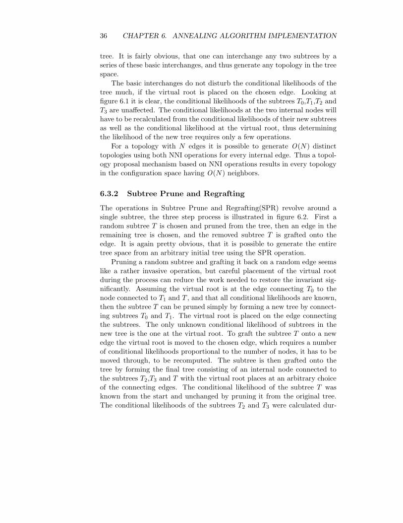
The operations in Subtree Prune and Regrafting(SPR) revolve around asingle subtree, the three step process is illustrated in figure 6.2. First arandom subtree T is chosen and pruned from the tree, then an edge in theremaining tree is chosen, and the removed subtree T is grafted onto theedge. It is again pretty obvious, that it is possible to generate the entiretree space from an arbitrary initial tree using the SPR operation.
Pruning a random subtree and grafting it back on a random edge seemslike a rather invasive operation, but careful placement of the virtual rootduring the process can reduce the work needed to restore the invariant sig-nificantly. Assuming the virtual root is at the edge connecting T0 to thenode connected to T1 and T , and that all conditional likelihoods are known,then the subtree T can be pruned simply by forming a new tree by connect-ing subtrees T0 and T1. The virtual root is placed on the edge connectingthe subtrees. The only unknown conditional likelihood of subtrees in thenew tree is the one at the virtual root. To graft the subtree T onto a newedge the virtual root is moved to the chosen edge, which requires a numberof conditional likelihoods proportional to the number of nodes, it has to bemoved through, to be recomputed. The subtree is then grafted onto thetree by forming the final tree consisting of an internal node connected tothe subtrees T2,T3 and T with the virtual root places at an arbitrary choiceof the connecting edges. The conditional likelihood of the subtree T wasknown from the start and unchanged by pruning it from the original tree.The conditional likelihoods of the subtrees T2 and T3 were calculated dur-

6.3. TOPOLOGY CHANGING OPERATIONS 37
T0
T1
T0
T1
T T
TT
T2
T3
T2
T3
Figure 6.2: subtree prune and regraft. The process of pruning a subtreeT from a tree and regrafting it is carried out in three steps. The dashedlines indicate the location of the virtual roots, and T0-T3 represent generalsubtrees. The virtual root is initially placed at the connecting edge of oneof the remaining subtrees. The subtree T is then pruned off, and a new treeformed by connecting the remaining subtrees. The virtual root is placedon the connecting edge. The virtual root is then moved to the regraft edge.Finally the subtree T is grafted onto the edge, the virtual root can be placedarbitrarily. The majority of the work required to restore the invariant is doneduring the movement of the virtual root.
38 CHAPTER 6. ANNEALING ALGORITHM IMPLEMENTATION
ing the movement of the virtual root in step two, thus the only conditionallikelihood needed to restore the invariant is the one at the added internalnode and at the virtual root.
For a topology with N edges it is possible to generate O(N2) distincttopologies using SPR operations. A quick way to see this is to choose twoedges, one edge is the regraft edge, the other edge defines two subtrees, oneof which contains the regraft edge, the other can be used as the subtree tobe pruned. There are O(N2) ways to choose two edges in the tree, thususing SPR operations results in every topology in the configuration spacehaving O(N2) neighbors.
6.3.3 Tree bisection and recombination
The operations in Tree Bisection and Recombination(TBR) are based onbreaking and joining trees by adding and removing connecting edges asshown in figure 6.3. First an edge between internal nodes is selected andremoved. Then two smaller trees are formed by joining the two subtrees ateach of the internal nodes. An edge is then selected in each of the smallertrees, and the trees are joined by inserting an internal node in the chosenedges as well as a connecting edge between the added nodes. The overallresult is a potentially radical change of tree topology, and as such it is nothard to see, that TBR can generate the entire tree space.
Despite the rather dramatic changes to the topology it is possible torestore the invariant by careful placement of virtual roots during the process.Assuming the virtual root is initially at the edge chosen for removal infigure 6.3 and all conditional likelihoods of subtrees known, then virtualroots can be placed at the edges connecting the subtrees T0-T1 and T2-T3
requiring only the conditional likelihoods at these roots to be calculatedfrom those of the subtrees as these smaller trees satisfy the same invariantas the parent tree. Each virtual root in the smaller trees must then bemoved to the edges chosen for the recombination of the trees, which requirea number of conditional likelihoods proportional to the sum of nodes the twovirtual roots must be moved through. Defining the virtual root of the finaltree to be at the central edge, then the invariant can be restored by merelycalculating the conditional likelihoods of the two added internal nodes andat the virtual root, since the conditional likelihoods of all the subtrees weredetermined during the movement of the virtual roots in the smaller trees,which brings the number of conditional likelihoods needed to be calculatedduring the TBR operation to five, two in step one and three in step three,plus a number proportional to the sum of distances the virtual roots in

6.3. TOPOLOGY CHANGING OPERATIONS 39
T0
T1
T2
T3
T0
T1
T2
T3
T4
T5
T6
T7
T4
T5
T6
T7
Figure 6.3: Tree bisection and recombination. The process of recombininga tree takes place in three steps. The dashed lines indicate the location ofthe virtual roots, and T0-T7 represent general subtrees. The virtual rootis initially placed at the bisection edge. First the bisection edge and thenodes, it is incident on, are removed resulting in two trees, each with avirtual root at the edges connecting its two subtrees. Then the virtual rootsare moved to the recombination edge in each tree, and a node is inserted ineach recombination edge and connected. The virtual root of the resultingtree is placed at the connecting edge. The majority of the work required torestore the invariant is done during the movement of the virtual roots.

40 CHAPTER 6. ANNEALING ALGORITHM IMPLEMENTATION
the smaller trees have to be moved. While the cost of maintaining theconditional likelihoods is fairly significant, it is of course still considerablysmaller than calculating them all from scratch.
There is no simple expression for the number of distinct topologies pos-sible by applying a single TBR operation on a topology. It is obviouslypossible to choose the bisection edge and recombination edges in O(N3)ways, but a lot of TBR operations give rise to the same topologies, makingthe actual number far smaller. The number of distinct topologies is at leastas large as in the case of SPR operations, since they are a subset of the TBRoperations corresponding to the case, where one of the virtual roots in thesmaller trees is not moved.
6.3.4 Discussion
Each of the three topology changing operations define a neighbor relationresulting in a connected configuration space, however the number of neigh-bors each configuration has varies for the three types of operations as doesthe work required to maintain the invariant. Having many neighbors makesit less probable for a simulation to get stuck in local maxima. On the otherhand having a large number of neighbors complicates the exploration ofthe neighborhood. In the extreme case, where every pair of configurationsare neighbors, there are no local maxima to get stuck in, but exploring theneighborhood of any configuration corresponds to an exhaustive search ofthe configuration space.
NNI operations only result in relatively small changes to topologies,which can pose a problem, if the simulation gets stuck in a local maxi-mum, since it could easily require many downhill NNI moves to escape theregion. Both SPR and TBR operations can result in large changes in topolo-gies, and thus are able to to escape in much fewer steps. The neighborhoodaround each topology is also much larger, when using SPR or TBR opera-tions in the topology proposal mechanism, making local maxima much lessabundant than in the case of NNI operations, but the large neighborhoodcan make finding an improving operation difficult. The difference betweenusing SPR and TBR operations is much less clear. The neighborhoods areof comparable size, but the work required to maintain the invariant appearson average to be larger for the more complex TBR operations than for SPR.
The topology operations used here is a union of NNI and SPR operationswith variable probability, enabling the topology proposal mechanism to workas anything between pure NNI moves to SPR moves. For both types ofoperations only a single topology in the neighborhood is examined, there

6.4. OPTIMIZATIONS 41
isn’t much work saved by exploring say two neighbors as opposed to takingtwo steps, the majority of the work is in the branch length optimizationof the proposed topologies. Secondly, there isn’t any reason to expect thesecond topology to be on average any better than the first.
6.4 Optimizations
The majority of time spent during a simulation is spent evaluating the likeli-hood function during branch length optimization, thus it is the most obviousplace for optimizations. To improve performance one must either reduce thetime needed to evaluate the likelihood or reduce the number of times thefunction is evaluated.
6.4.1 Subtree equivalence vectors
It is possible to reduce the amount of work required to evaluate the likelihoodfunction by making use of the independence of the individual sites in alikelihood vector and reuse quantities from calculations at one site at othersites. One approach to reuse is by means of ’subtree equivalence vectors’[25]. The idea is to keep track of how many times a column is repeatedin the alignment containing only sequences corresponding to the leaves ofthe subtree, the conditional likelihood is being calculated for and simplyreuse values wherever possible. Subtree equivalence vectors for leaves aredetermined directly from the corresponding sequences having one entry foreach letter occurring in the string.
Figure 6.4 illustrates how a subtree equivalence vector is calculated fromtwo subtrees. In the example the subtrees are leaves and the conditionallikelihood vectors derived directly from the sequences. Equivalence vectorsneed an entry for each distinct letter in the corresponding sequences, whichin this case turns out to be three and four respectively. The sequence rep-resenting the likelihood vector of the parent is determined site for site bycombining the corresponding letters of the left and right child vector as in-dicated by the dashed lines. The parent sequence is a sequence over theproduct of the alphabets of the child sequences. In the example the equiva-lence vector of the parent has only six elements, which need to be calculated,compared to the sixteen entries in the likelihood vector. The reduction innumber floating point operations is considerable, however it does require afair bit of bookkeeping to use subtree equivalence vectors.
One obvious problem is the rapid growth of the alphabet with the size ofthe subtree. The size of the alphabet can be limited to the size of the

42 CHAPTER 6. ANNEALING ALGORITHM IMPLEMENTATION
A U G C A A A G G A A A U U U U
A U G C
A U G C A A A G G A A A U U U UA U G A A G A A A U UG G A U U
AA
UU
GG
CG
AG
GA
A U G A A G A A A U UG G A U U
A U G
Figure 6.4: Subtree equivalence vectors. An example of how a likelihoodvector is calculated from the likelihood vectors of two subtrees using equiv-alence vectors. Essentially the entries in a likelihood vector act as keys withthe corresponding values stored in a subtree equivalence vector.

6.4. OPTIMIZATIONS 43
alphabet of the sequences in the underlying multiple alignment by onlyreusing values for sites, where all leaves in the subtree have the same letter.In this example the number of calculated entries remains six. Topologychanging operations and movement of the virtual root also become morecomplex, because they require the equivalence vectors to be recalculated,but benefit far less than branch optimizations, where the bookkeeping isdone once, and the benefit realized many times.
The speedup gained depends on how much the equivalence vectors can becompacted, but the amount of work saved can be considerable, Stamatakis[25]reports speedup of 30%-60% depending on data.
6.4.2 Partial tree optimization
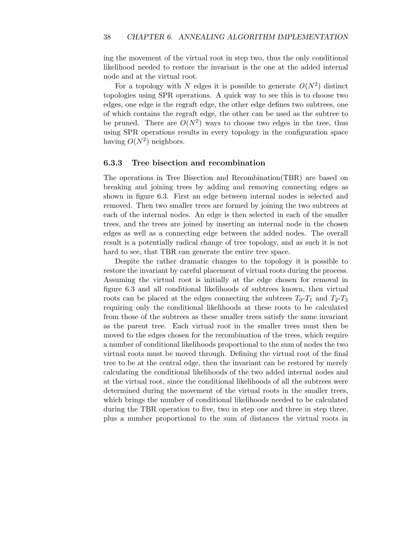
Reducing the number of branches considered for branch length optimizationis in theory hard due to the coupling between them, a change to any branchwill have an impact on all other branches, however the coupling is generallyconsidered weak, thus the effect of changes in distant branches will decreaserapidly. Secondly, branch optimization must be performed using numericalmethods and as such, the branch lengths and the likelihoods of trees are onlyapproximately optimal. Given an optimized tree, the impact of a topologychange is global, but there is little point in optimizing the branches, wherethe effect is smaller than the precision of the numerical method. In practiceit is difficult to give an estimate of how wide an area of a tree must beoptimized after a topology change without resorting to heuristics and trialsimulations.
The simplest such heuristic is to use a cut off distance from the virtualroot used in the topology changing operation as illustrated in figure 6.5.The work involved in moving the virtual root around is small compared tothe actual work required to optimize the branches, but the optimization ofthe branches can be expected to require several sweeps, before convergenceis reached, thus optimizing the branches in the order given by a boundeddepth-first traversal from the virtual root is preferable, as it leads to thevirtual root visiting each branch twice, which is the lowest possible.
6.4.3 Discussion
Subtree equivalence vectors is basically a compression technique and as suchit does not affect the value of the likelihood function being calculated. Thespeedup from subtree equivalence vectors is fairly small, and their imple-mentation is fairly complex due to the the booking required. Optimizing
44 CHAPTER 6. ANNEALING ALGORITHM IMPLEMENTATION
Figure 6.5: The number of branches to be optimized after a topology changecan be reduced by only including branches with a maximum depth from thevirtual root. The dashed line indicates the location of the virtual root,the dashed circle indicates the maximum depth. The branches in full areincluded in the branch length optimization.

6.5. PARALLELIZATION 45
only a subset of the branches on the other hand will have an impact onthe likelihood function. The implementation is trivial and the speedup forlarge trees should be very large. With partial tree optimization the costof optimizing a tree after a topology change is essentially independent ofthe size of the tree. Of the two optimizations considered here, only par-tial tree optimization was implemented due to its larger speedup and easierimplementation.
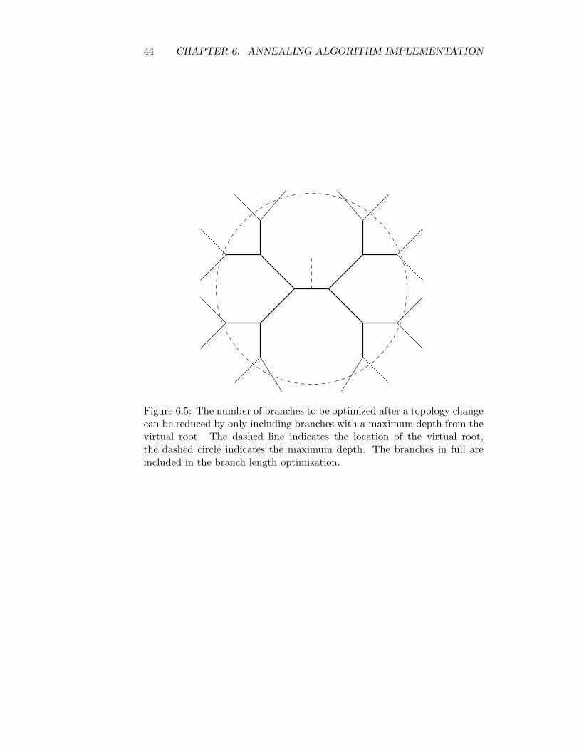
6.5 Parallelization
Finding the optimal phylogenetic tree for a large multiple alignment bymeans of simulated annealing is computationally very demanding both interms of memory and time required for the simulations to reach convergence.It is not realistic to hope the rapid improvement of hardware will overcomethese problems in the foreseeable future, since the growth of sequence datais considerably faster than improvements in hardware. Parallelization hasbeen widely used in the the field of phylogenetics as a means to find largerand better trees, and parallel versions in one form or other exist of manyprograms.
There are two obvious approaches to achieving parallelism in the anneal-ing algorithm; the calculation of likelihood vectors and the exploration of theneighborhood of the current configuration by the topology proposal mecha-nism. It is difficult to gauge the advantages of one over the other a priori,however a number of rules of thumb have been proposed by Pancake[20].The parallel version is to run on a cluster or network of workstations usingMPI, both choices reflect the de facto standard for parallel programs[1].
6.5.1 Parallelization of likelihood vector calculation
The calculation of each entry in a likelihood vector is independent of the en-tries due to the site independent nucleotide substitution model chosen. Onlywhen the likelihood of a tree is calculated are all the entries required. Thework needed to calculate each entry is fairly small, however it is identicalfor each entry, and the entries in a likelihood vector for a typical large treenumber in the thousands. This places the algorithm in the fully synchronouscategory, and according to the rules of thumb one can only expect reason-able performance in terms of speedup on a small cluster or shared memoryarchitectures. However the serial part of the algorithm is tiny compared tothe parallel part and independent of the size of the problem, while the par-allel part grows with the length of the sequences in the multiple alignment.
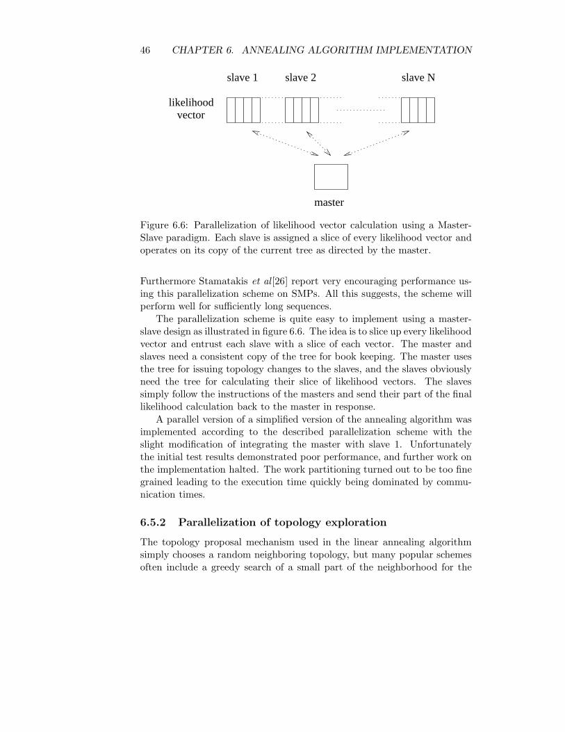
46 CHAPTER 6. ANNEALING ALGORITHM IMPLEMENTATION
slave 1
master
slave 2 slave N
likelihoodvector
Figure 6.6: Parallelization of likelihood vector calculation using a Master-Slave paradigm. Each slave is assigned a slice of every likelihood vector andoperates on its copy of the current tree as directed by the master.
Furthermore Stamatakis et al [26] report very encouraging performance us-ing this parallelization scheme on SMPs. All this suggests, the scheme willperform well for sufficiently long sequences.
The parallelization scheme is quite easy to implement using a master-slave design as illustrated in figure 6.6. The idea is to slice up every likelihoodvector and entrust each slave with a slice of each vector. The master andslaves need a consistent copy of the tree for book keeping. The master usesthe tree for issuing topology changes to the slaves, and the slaves obviouslyneed the tree for calculating their slice of likelihood vectors. The slavessimply follow the instructions of the masters and send their part of the finallikelihood calculation back to the master in response.
A parallel version of a simplified version of the annealing algorithm wasimplemented according to the described parallelization scheme with theslight modification of integrating the master with slave 1. Unfortunatelythe initial test results demonstrated poor performance, and further work onthe implementation halted. The work partitioning turned out to be too finegrained leading to the execution time quickly being dominated by commu-nication times.
6.5.2 Parallelization of topology exploration
The topology proposal mechanism used in the linear annealing algorithmsimply chooses a random neighboring topology, but many popular schemesoften include a greedy search of a small part of the neighborhood for the

6.5. PARALLELIZATION 47
slave 1
master
slave 2 slave N
topologyproposals top 1 top 2 top N
Figure 6.7: Parallelization of topology exploration using a Master-Slaveparadigm. Each slave maintains a copy of the current tree and sends pro-posals for new topologies to the master for evaluation.
best topology; the one most likely to be accepted in the Metropolis step.A greedy search of the neighborhood of a topology falls into the categoryof loosely synchronous problems, since the time required to explore eachtopology varies. However the only synchronization point of the algorithmis the selection of the best candidate, and each candidate requires branchoptimization to be performed on at least a part of the corresponding tree,which for even modest sized trees involves many thousands of floating pointoperations. Pancake’s rules of thumb suggest, there is potential for goodperformance, if the time required to optimize each candidate is sufficientlylong, and Stamatakis[25] reports good performance using a parallelizationscheme based on a distributed greedy search for a good topology proposal.
Parallel exploration of a neighborhood is fairly straight forward usinga master-slave design as illustrated in figure 6.7, but a few points need tobe addressed, first of all the division of labor. One possibility is to let themaster select a distinct topology for each slave and them distribute themto the slaves. It avoids the risk of duplicate work at the cost of havinga longer serial part of the algorithm. Alternatively selection of topologiescould be left to the slaves. Duplication of work is clearly not productive,but the neighborhood of a topology is O(N2) in the size of the tree, ifone includes subtree prune and regraft operations, thus the probability ofrandomly choosing the same topology twice or more quickly becomes remoteeven in the case of many slaves. In other words, communication overheadis likely to become a bottleneck long before duplication of work becomes
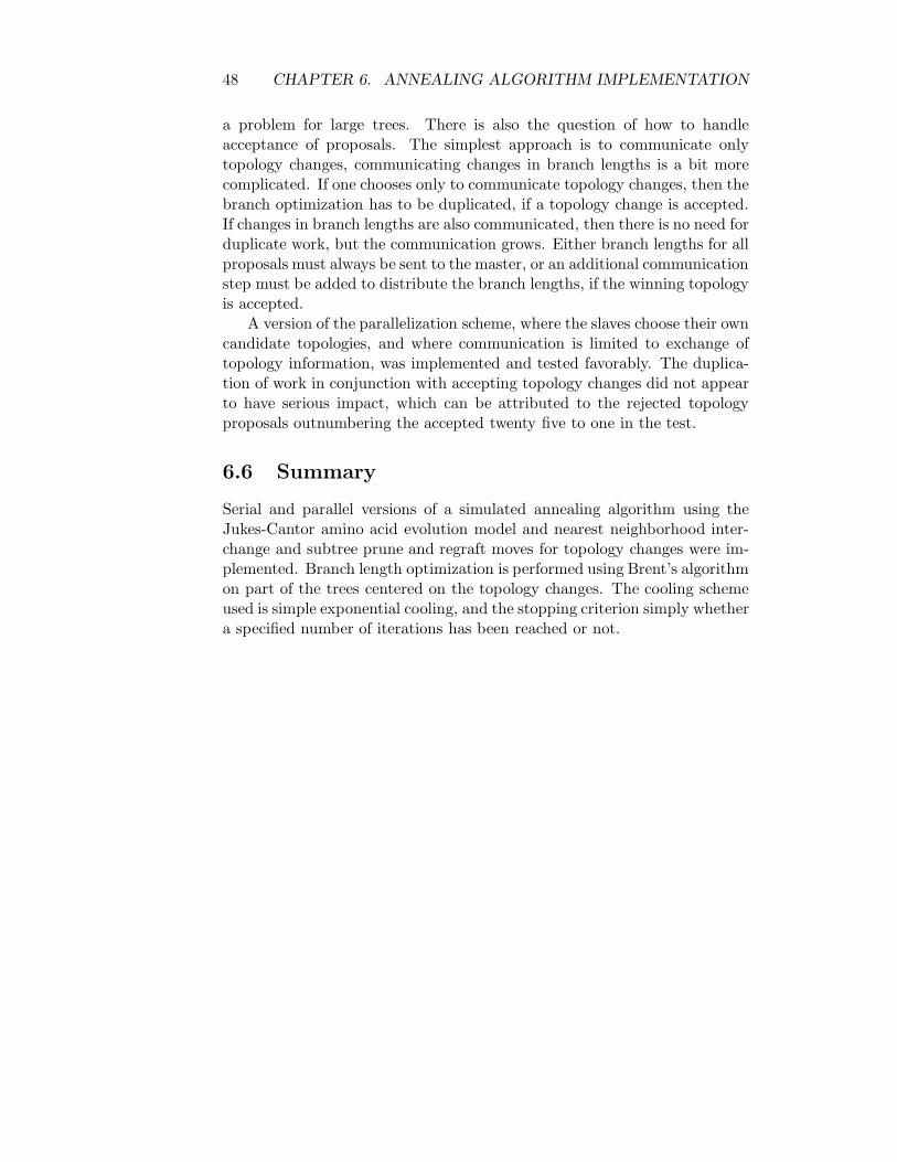
48 CHAPTER 6. ANNEALING ALGORITHM IMPLEMENTATION
a problem for large trees. There is also the question of how to handleacceptance of proposals. The simplest approach is to communicate onlytopology changes, communicating changes in branch lengths is a bit morecomplicated. If one chooses only to communicate topology changes, then thebranch optimization has to be duplicated, if a topology change is accepted.If changes in branch lengths are also communicated, then there is no need forduplicate work, but the communication grows. Either branch lengths for allproposals must always be sent to the master, or an additional communicationstep must be added to distribute the branch lengths, if the winning topologyis accepted.
A version of the parallelization scheme, where the slaves choose their owncandidate topologies, and where communication is limited to exchange oftopology information, was implemented and tested favorably. The duplica-tion of work in conjunction with accepting topology changes did not appearto have serious impact, which can be attributed to the rejected topologyproposals outnumbering the accepted twenty five to one in the test.
6.6 Summary
Serial and parallel versions of a simulated annealing algorithm using theJukes-Cantor amino acid evolution model and nearest neighborhood inter-change and subtree prune and regraft moves for topology changes were im-plemented. Branch length optimization is performed using Brent’s algorithmon part of the trees centered on the topology changes. The cooling schemeused is simple exponential cooling, and the stopping criterion simply whethera specified number of iterations has been reached or not.

Chapter 7
Tree Update Implementation
The implementation of the proposed heuristic for updating phylogenetictrees falls in three natural steps; identification of leaves to be added orremoved, distance calculation and the actual update of the phylogenetictree. In this chapter we give detailed descriptions of the design choices forthe implementation of each of the three steps involved in constructing aphylogenetic tree for one multiple alignment based on another alignmentand a tree topology for this other alignment.
7.1 Mapping an old multiple alignment to a new
The file format used here for multiple alignments is simply a sequence ofstrings. Each sequence is identified by its position in the sequence, thus itis necessary to not only identify strings to be added or removed but also tomap the identifiers for the common set of strings. Sequences in a multiplealignment usually contain gaps, which need to be removed before a mappingbetween sequences from two alignments using a dictionary is possible.
There are several ways to compute a map between two sets of strings,the approach used here is simply to create a dictionary containing one setand look up the strings of the other set. The data structure used for thedictionary is a compressed trie, where the leaves hold both the tail of a stringand the associated value. The choice of a trie reflects a compromise betweenease of implementation and running time, which in all cases is expected to beinsignificant compared to the time required by the corresponding annealingruns to converge.
Using a trie constructs the map in time O(NM log a), where N is thesize of the combined sets, M is the length of the strings, and a is the size of
49

50 CHAPTER 7. TREE UPDATE IMPLEMENTATION
c ga
c
a
u
u$
$u
ga
$
c
$
gu a
$
Figure 7.1: Example of a Compact Trie containing the strings; uggau, uggca,uggcu, uacca and uacgu. The dollar signs indicate end of string markers.
the alphabet.Multiple alignments can take up a considerable amount of memory, but
this problem is easily overcome simply by distributing the sequences to anumber of slaves, each maintaining a smaller dictionary as illustrated infigure 7.2. Obviously this only increases the size of alignments, which canbe compared, it does not improve the running time.
Both sequential and parallel versions of the alignment comparisons algo-rithms were implemented, however only the sequential version was actuallyused, since the trees, for which simulated annealing runs could be convergedin reasonable time, turned out to be a lot smaller than expected, and themultiple alignments based on real data contained a great deal of gaps, re-sulting in the set of strings in the alignment taking up significantly less spacethan the alignment.
7.2 Distance matrix
The calculation of the distances needed to perform updates on an existingphylogenetic tree is straight forward. The distance measure used is the oneimplied by the Jukes-Cantor model which is also used for branch length op-timization in the simulated annealing algorithm. The heuristic for updatinga tree requires the distance between every sequence unique to the new mul-tiple alignment and all other sequences in the new alignment to be known.The distances between sequences common to the old and new alignmentare not needed, as the corresponding leaves in the tree build from the oldalignment are not touched. The required parts correspond to region 2 and 3in figure 7.3.
How large a part of the full distance matrix, which has to be calculated,

7.2. DISTANCE MATRIX 51
slave 1
master
slave 2 slave N
Tries
Figure 7.2: Distribution of the dictionary using a master slave paradigm.Each slave maintains a trie with a subset of the full dictionary allowing alarger dictionary than the memory of any of the slaves permit. Look-ups areperformed simultaneously by all slaves and the result sent to the master.
1 2
3
Common Added
Com
mon
Add
ed
Sequences
Sequ
ence
s
Figure 7.3: Calculation of a partial distance matrix. The heuristic for up-dating an existing phylogenetic tree requires the distance between each se-quence to be added and all other sequences in the new alignment. Thedistance measure is symmetric, thus only matrix entries in regions 2 and 3need to be calculated.

52 CHAPTER 7. TREE UPDATE IMPLEMENTATION
depends on how much the alignments have in common of course, but theheuristic assumes a large degree of similarity between the optimal trees foreach alignment, and as such implies, that only a small part of the distancematrix is required. There is no analytical form for the distance betweentwo sequences in the model used as it allows for sampling errors and thelike. Instead the distances have to be determined by numerical methods.The approach used here is simply to build trees of size two for each dis-tance to be calculated. The distances between the pairs of sequences arethen determined by performing branch length optimizations on the branchesconnecting the corresponding nodes.
Calculating the required entries in a distance matrix for a large multiplealignment can be a demanding task; the sequences must be converted tolikelihood vectors, which take up a lot more memory than sequences, andgaps can no longer be ignored. Furthermore the distances must be calculatedwith high accuracy requiring many iterations, and the number of distanceis in worst case quadratic in the number of sequences.
The calculations of distances are independent of each other, thus it isfairly straight forward to overcome the memory issues using caching tech-niques, however it is possible to do better through parallelization. One sim-ple parallelization scheme is to distribute the added sequences on a numberof slaves, stream the entire alignment against them and have the slaves sendthe distances to a master. This is quite efficient in terms of memory, butit does not perform well, if the alignment is large but only few sequenceshave been added, nor does it work well if the ratio of added sequences islarge, since the alignment effectively has to be streamed twice; once duringthe distribution step and once during the calculation step. Dividing thesequences of the alignment between the slaves instead addresses both issues;the number of sequences for alignments of significant size makes load bal-ancing easier, secondly the “added” sequences do not have to be streamedby the master, they can be retrieved from whichever slave happens to haveit in memory.
A serial version and the second parallel version of the algorithm wereimplemented and both used to calculate the distance matrices used in theexperimental section. The parallel version proved most useful for calculatingthe distance matrices used by the Neighbor-Joining algorithm due to thelarge number of entries. The size of the alignments, which the simulatedannealing algorithm could converge in reasonable time, turned out not topose much of a problem for distance matrix calculation.

7.2. DISTANCE MATRIX 53
master
likelihoodvectors
slaves
broadcast
group
Figure 7.4: Parallelization of the distance matrix calculation. The masterreads and distributes the sequences to the slaves round-robin and then waitsfor the slaves to send results back. The “added” sequences are broadcastedby the responsible slave as needed. Communication between master andslaves is asynchronous, while the broadcasts between slaves is synchronous.The order in which the “added” sequences are broadcast is determined fromthe mapping between the old and new multiple alignments and broadcastto the slaves along with other book keeping information.

54 CHAPTER 7. TREE UPDATE IMPLEMENTATION
best edge
active
edges
heap
vector
Figure 7.5: Prim-Jarnık spanning tree algorithm using a heap. The setof active edges is stored in an augmented heap, which, aside from normalheap operations, supports read and removal of any element on the heap.The second data structure used in the implementation is a vector with anelement for each node containing either the index of the edge in the activeset incident on the node or a place holder, if there is no such edge.
7.3 Updating the tree
The update of a phylogenetic tree is quite simple given both a mappingbetween the old and the new multiple alignment and a distance matrixfor the new alignment. Update of the tree can be done in three basic steps;pruning of leaves to be removed, renumbering of common leaves and additionof new leaves as described in chapter 4. Pruning and renumbering leavesrequires little more than traversal of a list of edges, while adding new leavesinvolves finding the minimum spanning tree of a carefully constructed graphusing the Prim-Jarnık spanning tree algorithm.
The spanning tree algorithm used is a slightly modified version of thePrim-Jarnık spanning tree algorithm as cast by Goodrich and Tamassia[18].The key data structures used are an augmented heap and a vector with anentry for each node containing either a place holder or the position on theheap of the edge incident on the node as illustrated in figure 7.5.
The algorithm finds the minimum spanning tree by growing a cloudfrom a starting node, each node inside the cloud is covered by an edge inthe spanning tree, nodes outside the cloud are not. The set of edges onthe heap consists of the shortest edges connecting each node outside thecloud to a node inside. The vector is simply a map between nodes outside

7.3. UPDATING THE TREE 55
the cloud and an edge on the heap. It is straight forward to see, that theset of edges on the heap, after every zero weight edge in the constructedgraph has been added, will consist of edges between a leaf in the old treeand a leaf to be added. The addition of zero weight edges is not used toupdate the phylogenetic tree, thus it is possible to omit the zero weightedges and nodes corresponding to internal nodes in the phylogenetic tree, ifone initializes the heap and vector with the proper values. A simple way toperform this initialization is to treat every node corresponding to a leaf inthe phylogenetic tree as a starting point for the Prim-Jarnık algorithm.
Only a serial version of the algorithm for updating phylogenetic trees wasimplemented and used in experiments. A parallel version did not make a lotof sense, since the algorithm is fast, and the memory use is quite modest.

56 CHAPTER 7. TREE UPDATE IMPLEMENTATION

Chapter 8
Experiments
In this chapter we present a series of experiments testing the proposed heuris-tic for constructing phylogenetic trees and experiments testing the imple-mented annealing algorithm. The reference used when testing the heuristicis the Neighbor-Joining algorithm.
The multiple alignment used in the experiments in this chapter wereunless otherwise noted based on a multiple alignment of highly conservedregions of ribosomal RNA for archaea and eukaryots extracted from the ARBdatabase. The alignments used in the experiments had to be reduced in sizefor the implemented annealing algorithm to be able to handle them, whichwas done simply by picking the desired number of entries in the originalalignment and ignore the rest.
The topology proposal mechanism used in the simulations made use ofNearest Neighbor Interchange and Subtree Prune and Regraft moves withequal probability. The likelihood results are given as log likelihoods, andevery simulation was repeated five times and unless otherwise noted simplyaveraged to gain at least a little confidence in the results. The reruns wereperformed on different alignments of same size to compensate for bias inthe data. Five experiments is a small number to build statistics on, but thedeviation of the results in properly converged cases proved to be quite small,which somewhat justifies the small number.
8.1 Tree construction using Neighbor-Joining
A set of simulations were carried out using Neighbor-Joining trees as start-ing points to illustrate the problem of relying on the Neighbor-Joining algo-rithm for an initial topology for large trees. The simulations were allowed
57
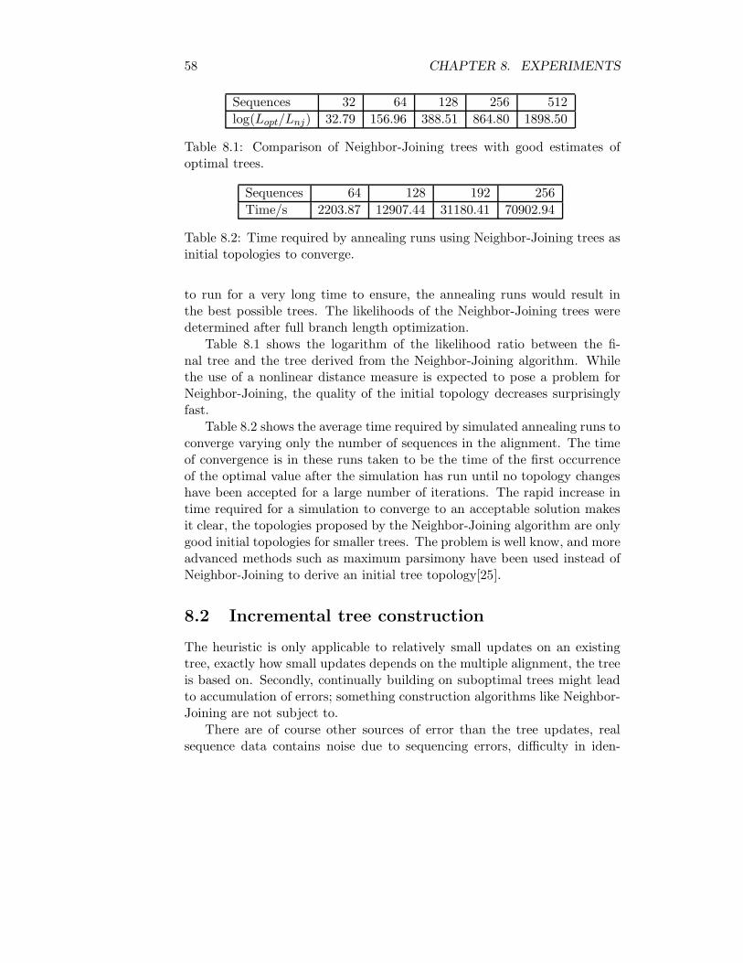
58 CHAPTER 8. EXPERIMENTS
Sequences 32 64 128 256 512
log(Lopt/Lnj) 32.79 156.96 388.51 864.80 1898.50
Table 8.1: Comparison of Neighbor-Joining trees with good estimates ofoptimal trees.
Sequences 64 128 192 256
Time/s 2203.87 12907.44 31180.41 70902.94
Table 8.2: Time required by annealing runs using Neighbor-Joining trees asinitial topologies to converge.
to run for a very long time to ensure, the annealing runs would result inthe best possible trees. The likelihoods of the Neighbor-Joining trees weredetermined after full branch length optimization.
Table 8.1 shows the logarithm of the likelihood ratio between the fi-nal tree and the tree derived from the Neighbor-Joining algorithm. Whilethe use of a nonlinear distance measure is expected to pose a problem forNeighbor-Joining, the quality of the initial topology decreases surprisinglyfast.
Table 8.2 shows the average time required by simulated annealing runs toconverge varying only the number of sequences in the alignment. The timeof convergence is in these runs taken to be the time of the first occurrenceof the optimal value after the simulation has run until no topology changeshave been accepted for a large number of iterations. The rapid increase intime required for a simulation to converge to an acceptable solution makesit clear, the topologies proposed by the Neighbor-Joining algorithm are onlygood initial topologies for smaller trees. The problem is well know, and moreadvanced methods such as maximum parsimony have been used instead ofNeighbor-Joining to derive an initial tree topology[25].
8.2 Incremental tree construction
The heuristic is only applicable to relatively small updates on an existingtree, exactly how small updates depends on the multiple alignment, the treeis based on. Secondly, continually building on suboptimal trees might leadto accumulation of errors; something construction algorithms like Neighbor-Joining are not subject to.
There are of course other sources of error than the tree updates, realsequence data contains noise due to sequencing errors, difficulty in iden-

8.2. INCREMENTAL TREE CONSTRUCTION 59
Increase/% Time/s log Lstepwise σ(log Lstepwise)
10 24577.28 -12521.76 13.6420 12649.61 -12555.18 28.6930 10653.59 -12590.16 46.2540 7843.44 -12607.04 23.92
Table 8.3: Stepwise construction of trees with 256 sequences. The numberof iterations between additions of sequences was five times the number ofsequences in the current tree.
Increase/% Time/s log Lstepwise σ(log Lstepwise)
10 45677.78 -12494.22 1.0620 24783.87 -12522.04 25.5730 18521.75 -12527.22 39.2940 15373.14 -12591.54 54.01
Table 8.4: Stepwise construction of trees with 256 sequences. The numberof iterations between additions of sequences was ten times the number ofsequences in the current tree.
tifying regions with strong phylogenetic signal and even in the underlyingmultiple alignment. These sources of error affect sequences to a varying de-gree potentially causing the overall quality of a subset of the data to dependgreatly on the actual sequences in the subset, which would make comparisonbetween trees of different sizes difficult, and could cause the exact order, inwhich sequences are added, to be significant. Adding the most noisy se-quences first would lead to more propagation of errors than adding the leastnoisy sequences first, thus the following experiments were carried out usingsimulated data. The data was constructed from a random string of lengthone hundred over a four letter alphabet and increased to the desired size bydoubling followed by mutation of each string in the old set.
8.2.1 The size of updates
Two series of experiments with repeated addition of sequences were made fordifferent rates of additions, in the first series the annealing algorithm is runon the tree after each addition for a number of iterations corresponding tofive times the size of the current tree, in the second series the number was tentimes the current tree size. The results can seen in table 8.3 and table 8.4.It is clear from the tables, that the relative growth ratio has a very large

60 CHAPTER 8. EXPERIMENTS
Sequences 64 128 192 256
log Lopt/Lstep 43.48 99.73 184.12 7.59
σ(log Lstep) 56.09 69.16 90.48 14.06
Table 8.5: Construction of trees by growing them 10% step by step. Thenumber of iterations between additions of sequences was ten times the num-ber of sequences in the current tree.
impact on the quality of the resulting tree in terms of likelihood, the effectof doubling the number of iterations during the convergence steps is alsoquite significant. The likelihood of the best tree produced is a mere 1 fromthe best value found by very long annealing runs on trees constructed byneighbor-joining, and the corresponding standard deviation is much smallerthan for any other simulation, which clearly indicates convergence. Theexperiments suggest, a good choice of parameters for this kind of stepwiseaddition would be to limit the growth ratio to 10% increases for each stepand iterate for ten times the number of sequences in the corresponding tree.
The log likelihoods and standard deviations are fairly systematic, thelarger the increases, the larger the deviation and the lower the likelihood,which is entirely to be expected. It is a little surprising, that doublingthe number of iterations in each step does not have greater impact on thedeviations. Looking at the log likelihoods it is interesting, that they growsomewhat regularly with increasing sizes of addition but make a jump toaround −12590 in both series. A probable cause for this is the algorithmgetting stuck in a local maximum. Given only a short time to escape sucha maximum and, assuming the subsequent additions of sequences does notnudge the algorithm out of the maximum, the probability of escape is quitesmall.
Summary
The conclusion is, that it seems possible to add a relatively large number ofnew sequences to an existing phylogenetic tree by inserting each sequencenext to the sequence, it is most similar to, without introducing too manyerrors.
8.2.2 Different sizes of trees
A series of experiments were made in order to test, if the guide line of 10%increases followed by an annealing run of a length corresponding to ten

8.3. UPDATING A PHYLOGENETIC TREE 61
times the size of the tree holds for different tree sizes. The results can beseen in table 8.5. The relatively large likelihood ratio and rapid increase issurprising, the ratio is growing more rapidly than the logarithm of likelihooditself, which suggests, the trees have not been properly converged before thenext sequences are added to the tree. This would result in an accumulationof error, since adding sequences to a poor tree is quite unlikely to yield agood starting point for converging a larger tree. The sudden decline in theratio and deviation for trees with 256 leaves is likely to be due to reachinga critical point, where enough errors have been corrected to make the treesgood starting points for convergence after addition of sequences, and thenumber of iterations during the convergence steps suddenly become morethan adequate. In hindsight the results are perhaps not so surprising. Theheuristic for adding sequences assumes there is a good tree to build on,which is far from the case when building from scratch.
Summary
The results of this simple stepwise construction algorithm suggest, that forthis data set adding sequences to the phylogenetic trees is relatively easy,and while propagation of error does take place as the tree is grown, treeupdates are not very sensitive to errors. Constructing a phylogenetic treestep by step in this fashion obviously isn’t the most efficient way to constructa tree, if the data set for the final tree is available at the start, there are farbetter choices such as using a disc covering method[22] followed by simulatedannealing. The results show, that trees can be increased in size by fairly largesteps, and that trees need not be strongly converged to avoid accumulationof error getting out of hand at a later stage.
8.3 Updating a Phylogenetic Tree
The addition of sequences to phylogenetic trees based on some very simpleand idealized multiple alignments was, in the previous subsection, shownto be quite feasible, but real alignments using real data can be expectedto contain much lower ration between the phylogenetic signal and noise.In this subsection addition and removal of sequences is explored on treesconstructed from alignments of ribosomal RNA for archaea and eukariotsfrom the ARB database.

62 CHAPTER 8. EXPERIMENTS
Removal of sequences from a Phylogenetic Tree
Figure 8.1 shows the average likelihoods of annealing runs using initial treesconstructed by the Neighbor-Joining algorithm and trees constructed byremoving extra sequences from a larger phylogenetic tree. The Neighbor-Joining trees were constructed from distance matrices using the same RNAevolution model as in the annealing run as distance measure. The initialtrees derived from larger trees were constructed by performing annealingruns on trees 10% larger trees until convergence and then remove the ex-tra sequences from the tree. The simulations were performed using fiverandomly chosen subsets of size 512 from the ARB database.
The figure quite clearly shows, that using a good phylogenetic tree for alarger multiple alignment as starting point by pruning leaves correspondingto sequences not found in the smaller alignment works very well. The de-rived trees are superior to those found after 40000 iterations starting fromNeighbor-Joining trees. The annealing runs using the derived trees yieldbetter topologies than the Neighbor-Joining simulations, which after even100000 iterations are still only very slowly catching up.
Addition of sequences to a Phylogenetic Tree
Figure 8.2 shows the average likelihoods of simulations with initial treesconstructed by respectively Neighbor-Joining and by adding sequences toa converged tree. The Neighbor-Joining trees were constructed as in theprevious set of simulations, and the initial trees derived from the smallertrees were constructed by performing annealing runs until convergence andthen insertion of the new sequences as neighbors to the closest sequencesin the tree using the distance matrix calculated for the construction of theNeighbor-Joining trees.
It is apparent from the graph, that the heuristic used for adding se-quences to existing trees does fairly well and certainly better than usingNeighbor-Joining to construct initial trees. The derived trees are better thanthe trees the simulations using Neighbor-Joining trees yield after 10000 it-erations. There is still a significant difference in likelihood between thesimulations after 100000, where the simulations using derived trees appearnicely converged and the Neighbor-Joining simulations clearly are not.
Summary
Using a phylogenetic tree derived from high quality trees based on data setssharing a large number of sequences with the current data set as a starting

8.3. UPDATING A PHYLOGENETIC TREE 63
-305000
-300000
-295000
-290000
-285000
-280000
0 20000 40000 60000 80000 100000
log
L
iterations
10% decreaseNeighbour-Join
Figure 8.1: Annealing runs using a Neighbor-Joining tree and a tree derivedby removing extra sequences from a converged but 10% larger tree
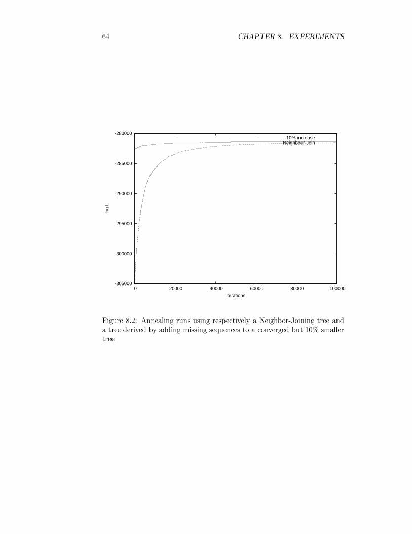
64 CHAPTER 8. EXPERIMENTS
-305000
-300000
-295000
-290000
-285000
-280000
0 20000 40000 60000 80000 100000
log
L
iterations
10% increaseNeighbour-Join
Figure 8.2: Annealing runs using respectively a Neighbor-Joining tree anda tree derived by adding missing sequences to a converged but 10% smallertree

8.4. PARALLELIZATION 65
point for a simulated annealing run works quite well. The derived treesproved to be vastly better than Neighbor-Joining trees thereby reducing thetime required for a simulation to find acceptable solutions. While the setsof annealing runs are far too small to make claims with any certainty, theysuggest, as much as half of the simulation time might be saved by usingknowledge gained from existing data sets.
Trees constructed only by removal of sequences are especially good initialtrees, trees constructed only by adding sequences are not quite as good initialtrees but still require only a fraction of the simulation time of Neighbor-Joining tree simulations. This is entirely to be expected, since, in a goodtree, the phylogenetic signal is strong and consistent in the sequences, andas such the removal of a few of these sequences should not give rise to largerearrangements in the remaining tree. Similarly the insertion of a few extrasequences are unlikely to cause rearrangements in an already well establishedtree, but the heuristic employed neglects long range effects, and while theeffects on the tree from the added sequences are expected to be small, thecombined effect of the rest of the tree on each added sequences need not besmall.
8.4 Parallelization
The purpose of the parallel version of the annealing algorithm was to makesimulations on larger data sets possible in part by making more memoryavailable for data and in part by speeding up simulations to make conver-gence feasible. The first objective was not reached, as the distribution ofthe data set on multiple nodes turned out to lead to a sharp increase ofthe simulation times in preliminary test. In this section the performanceof parallel exploration of the topology space is explored on alignments forarchaea and eukaryote ribosomal RNA from the ARB database.
8.4.1 Scaling
Figure 8.3 shows the average likelihoods for annealing runs starting fromNeighbor-Joining trees using 1, 2, 4 and 8 workers. The benefit of havingmore workers exploring the neighborhood of the current topology is fairlyclear, the simulations using the greatest number of workers are able to im-prove the topology much faster initially, and it converges to a topology witha higher likelihood than those of all other workers. The simulations us-ing just a single worker improve topologies noticeably slower and convergeto topologies inferior to those of simulations using several workers. This

66 CHAPTER 8. EXPERIMENTS
-86500
-86000
-85500
-85000
-84500
-84000
-83500
-83000
-82500
-82000
0 10000 20000 30000 40000 50000
log
L
iterations
1 worker 2 workers4 workers8 workers
Figure 8.3: Parallel annealing runs for 1, 2, 4, and 8 workers using identi-cal simulation parameters. All runs were performed using the same set ofNeighbour-Join start topologies for alignments with 128 sequences.

8.4. PARALLELIZATION 67
Topologies Lparallel Llinear
50000 -82281.4100000 -82278.5 -82279.8200000 -82267.9 -82277.6400000 -82266.0 -82272.5
Table 8.6: Parallel annealing runs for 1, 2, 4, and 8 workers and for twice,four times and eight times as long runs using identical simulation param-eters. Topologies is the number of topologies considered by the proposalmechanism, Lparallel and Llinear are the likelihoods of the best topologiesfound. All runs were performed using the same set of Neighbor-Joiningstart topologies for alignments with 128 sequences.
is entirely expected behavior considering the increased exploration of theneighborhood each extra worker adds.
The parallelization scheme used assumes a low chance of more than oneworker yielding an acceptable solution in any iteration, which the initialrapid increase in the likelihood for the simulations using eight workers sug-gests might not be the case. Having several acceptable solutions in everyiteration would cause the algorithm to become in a sense more greedy like ahill climbing algorithm than the serial version of the annealing algorithm asthe number of acceptable candidates in each iteration increases. This couldcause the parallel runs to have greater difficulty escaping local maxima.
A series of linear and parallel simulation runs were made to evaluate theeffect of using a slightly greedy algorithm in parallel runs, the results arelisted in table 8.6. The parallel runs were made using identical parameterssave the number of workers, while the linear runs were made with identicalparameters save the length of the run and the cooling frequency employed.The simulations show somewhat surprisingly, that the slightly greedier par-allel algorithm yields better results than the linear algorithm even when thelinear algorithm is allowed to run for a number of iterations correspondingto the number of workers times the length of the parallel simulation. Itseems, being greedy is a good idea, however even eight neighbors is a van-ishingly small subset of the neighborhoods for trees of this size, the chanceof all workers suggesting topologies, which could result in escaping a localmaxima, is still good for this few workers. The improved performance ofthe parallel algorithm can at least partly be attributed to greediness duringthe early parts of the simulation, where the topology is far from optimal,and picking the best proposal brings the current topology faster towards a

68 CHAPTER 8. EXPERIMENTS
maximum.
8.5 Local maxima
The results so far have been averages over many simulations on the samedata and the problem of local maxima fairly gracefully swept under the rug.It has however been a noticeable problem in most experiments, quite oftenmultiple simulations on the exact same data would converge to significantlydifferent values; a clear sign of simulations getting stuck in local maximadespite lengthy simulations starting from high temperatures and using slowcooling. The simplest solution to falling into local maxima is to repeatthe simulations several times in the hope, they wont all get stuck in localextrema. While this on average improves on the final result, it is also a bitwasteful, as a lot of time can be spent on simulations trying to escape alocal maximum despite the simulation having little hope of “catching up”with the best simulation on the data set.
It is possible to cut down on the wasted time by abandoning simulationsunlikely to yield a good result, these simulations could then be restarted us-ing a topology and temperature from another simulation as a starting point.This should result in more time being spent on simulations likely to improveon the current optimal topology and ultimately result in better results thana set of independent simulations. Figure 8.4 shows the simulations resultingin the best topology for two sets of five simulations on the same data set.One set consisted of five independent simulations, in the other set each ofthe five simulations were allowed to run until the next temperature decreaseafter which the likelihoods were compared and the simulation with the low-est likelihood restarted using one of the remaining topologies as startingpoint. Surprisingly, the graph does not show any significant benefit fromperiodically discarding the worst simulation. The number of simulations isa bit low, but this very simple form of restart appears to add nothing, theadded time for book keeping makes the result even more discouraging.
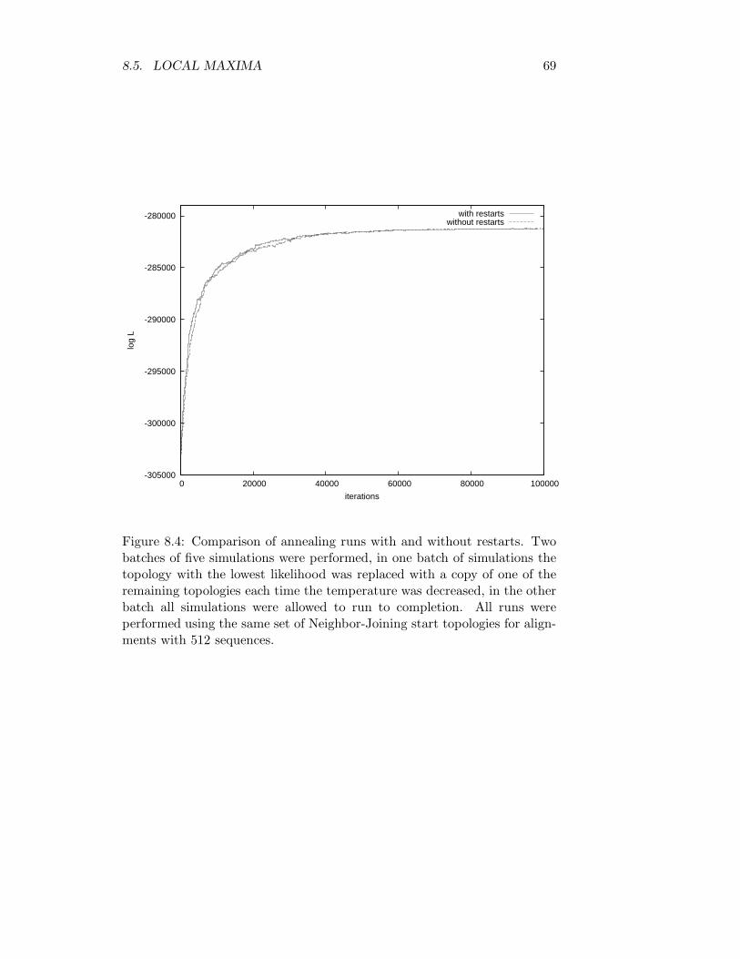
8.5. LOCAL MAXIMA 69
-305000
-300000
-295000
-290000
-285000
-280000
0 20000 40000 60000 80000 100000
log
L
iterations
with restartswithout restarts
Figure 8.4: Comparison of annealing runs with and without restarts. Twobatches of five simulations were performed, in one batch of simulations thetopology with the lowest likelihood was replaced with a copy of one of theremaining topologies each time the temperature was decreased, in the otherbatch all simulations were allowed to run to completion. All runs wereperformed using the same set of Neighbor-Joining start topologies for align-ments with 512 sequences.

70 CHAPTER 8. EXPERIMENTS

Chapter 9
Conclusion
A simple distance matrix based algorithm for updating existing phylogenetictrees was implemented in order to test, if construction of large trees could bespeeded up using prior knowledge about the topology of related trees, andan annealing algorithm for inferring phylogenetic trees based on maximumlikelihood implemented to improve on the updated trees.
A series of experiments were performed to test the consequences of in-cluding prior knowledge in this fashion. Experiments on simulated sequencedata showed, that trees making use of prior knowledge make much betterstarting points for annealing runs than trees constructed by the Neighbor-Joining algorithm. The amount of prior knowledge needed turned out to bequite high, addition or removal of roughly 10% seemed to work quite well forboth simulated and real sequence data. This makes the use of updated treesas starting points for further refinement by simulated annealing applicablemainly to situations, where one is interested in maintaining a phylogenetictree for a slowly changing data set, such as a growing sequence data base, ora sequence data base, where entries are slowly replaced with more accuratedata.
Implementation of the update algorithm proved quite easy, but the an-nealing algorithm turned out to be much more difficult than expected. It isquite easy to implement an annealing algorithm, but getting it to run fastenough to be able to handle large trees proved difficult, in addition thereis the problem of actually managing large data sets. Optimizations andheuristics had to be added along the way and even then, the size of multiplealignments, which could be handled in a reasonable amount of time wasunimpressive. The implemented topology proposal mechanism turned outto have serious problems escaping local maxima despite making use of both
71

72 CHAPTER 9. CONCLUSION
NNI and SPR moves, which leads to lengthy simulation runs or having torerun simulations many times to gain confidence in the resulting trees.
The topology proposal mechanism will have to be improved considerably,before larger data sets can be handled, and an external memory algorithmwill have to be employed, as the full data set will not fit in memory for theforeseeable future. Lastly a more efficient parallelization scheme will haveto be employed, the current scheme can not be expected to perform in thepresence of an external memory algorithm.

Bibliography
[1] Michael Allen Barry Wilkinson. Parallel Programming. Prentice Hall,1999.
[2] Matthew J. Brauer, Mark T. Holder, Laurie A. Dries, Derrick J. Zwickl,Paul O. Lewis, and David M. Hillis. Genetic algorithms and parallel pro-cessing in maximum-likelihood phylogeny inference. Mol. Biol. Evol.,19(10):1717–1726, 2002.
[3] Benny Chor, Michael D. Hendy, Barbara R. Holland, and David Penny.Multiple maxima of likelihood in phylogenetic trees:an analytic ap-proach. Mol. Biol. Evol., 17(10):1529–1541, 2000.
[4] Benny Chor and Tamir Tuller. Finding a maximum likelihood tree ishard. Journal of the ACM, 53, no. 5:722–744, September 2006.
[5] Sankoff D. Day W., Johnson D. The computational complexity of in-ferring rooted phylogenies by parsimony. Mathematical Biosciences,81:33–42, 1986.
[6] Dr. Isaax Elias. Settling the intractability of multiple alignment. Jour-nal of Computational Biology, 13(7):1323–1339, 2006.
[7] J. Felsenstein. Evolutionary trees from dna sequences:a maximum like-lihood approach. Journal of Molecular Evolution, 17:368–376, 1981.
[8] Joseph Felsenstein. Inferring Phylogenies. Sinauer Associates, Inc,2004.
[9] R. A. Fisher. On the mathematical foundations of theoretical statistics.Philosophical Transactions of the Royal Society of London, A 222:309–368, 1922.
73

74 BIBLIOGRAPHY
[10] D. G. Higgins and P.M. Sharp. Clustal: a package for performingmultiple sequence alignment on a microcomputer. Gene, 73:237–244,1988.
[11] J. Holland. Genetic algorithms and the optimal allocations of trials.SIAM Journal of Computing, vol 2(no 2):88–105, 1973.
[12] T. H. Jukes and C. R. Cantor. Evolution of protein molecules. In M. N.Munro, editor, Mammalian Protein Metabolism, volume III, pages 21–132. Academic Press, New York, 1969.
[13] S. Kirkpatrick, C. D. Gelatt, and M. P. Vecchi. Optimization by sim-ulated annealing. Science, Number 4598, 13 May 1983, 220, 4598:671–680, 1983.
[14] C. Lanave, G. Preparata, C Saccone, and G. Serio. A new methodfor calculating evolutionary substitution rates. Journal of MolecularEvolution, 20:86–93, 1984.
[15] Paul O. Lewis. A genetic algorithm for maximum-likelihood phylogenyinference using nucleotide sequence data. Mol. Biol. Evol., 15(3):277–283, 1998.
[16] Wolfgang Ludwig, Oliver Strunk, Ralf Westram, Lothar Richter, HaraldMeier, Yadhukumar, Arno Buchner, Tina Lai, Susanne Steppi, Gan-golf Jobb, Wolfram Forster, Igor Brettske, Stefan Gerber, Anton W.Ginhart, Oliver Gross, Silke Grumann, Stefan Hermann, Ralf Jost,Andreas Konig, Thomas Liss, Ralph Lußmann, Michael May, BjornNonhoff, Boris Reichel, Robert Strehlow, Alexandros Stamatakis, Nor-bert Stuckmann, Alexander Vilbig, Michael Lenke, Thomas Ludwig,Arndt Bode, and Karl-Heinz Schleifer. Arb: a software environmentfor sequence data. Nucleic Acids Research, 32(4):1363–1371, 2004.
[17] H. Matsuda. Protein phylogenetic inference using maximum likelihoodwith a genetic algorithm. Pacific Symposium on Biocomputing ’96,pages 512–523, 1996.
[18] Roberto Tamassia Michael T. Goodrich. Algorithm Design. John Wiley& Sons, Inc, 2002.
[19] J. Neyman. Molecular studies of evolution:a source of novel statisticalproblems. In S. S. Gupta and J. Yackel, editors, Statistical DecisionTheory and Related Topics, pages 1–27. Academic Press, New York,1971.

BIBLIOGRAPHY 75
[20] Cherri M. Pancake. Is parallelism for you? rules-of-thumb for computa-tional scientists and engineers. Computational Science and Engineering,Vol. 3(No. 2):18–37, 1996.
[21] R. C. Prim. Shortest connection networks and some generalizations.Bell Syst. Tech. J., 36:1389–1401, 1957.
[22] Usman W. Roshan, Bernard M. E. Moret, Tandy Warnow, andTiffani L. Williams. Rec-i-dcm3:a fast algorithmic technique for re-constructing large phylogenetic trees. Proceedings of the 2004 IEEEComputational Systems Bioinformatics Conference, 2004.
[23] N. Saitou and M. Nei. The neighbor-joining method: A new methodfor reconstructing phylogenetic trees. Molecular Biology and Evolution,4:406–425, 1987.
[24] R. R. Sokal and C. D. Michener. A statistical method for evaluat-ing systematic relationships. University of Kansas Science Bulletin,38:1409–1438, 1958.
[25] Alexandros Stamatakis. Distributed and Parallel Algorithms and Sys-tems for Inference of Huge Phylogenetic Trees based on the MaximumLikelihood Method. PhD thesis, Technische Universitat Munchen, Ger-many, October 2004.
[26] Alexandros Stamatakis, Michael Ott, and Thomas Ludwig. Raxml-omp: An efficient program for phylogenetic inference on smps. Pro-ceedings of 8th International Conference on Parallel Computing Tech-nologies (PaCT2005), Volume 3606 of Lecture Notes in ComputerScience:288–302, September 2005.
[27] Alexandrox Stamatakis. An efficient program for phylogenetic inferenceusing simulated annealing. In Proceedings of 19th IEEE/ACM Inter-national Parallel and Distributed Processing Symposium (IPDPS2005),High Performance Computational Biology Workshop, Proceedings onCD, Denver, Colorado, April 2005.
[28] Mike Steel. The maximum likelihood point for a phylogenetic tree isnot unique. Systematic Biology, 43(4):560–564, 1994.


![Computed Tomography Reconstruction Using Deep Image Prior ... · recently had great success in terms of reconstruction quality [2, 4, 15]. Three main classes are: end-to-end learned](https://img.pdfslide.net/doc/110x75/5f8552fb718984084234448f/computed-tomography-reconstruction-using-deep-image-prior-recently-had-great.jpg)


![Parsimonious Reconstruction of Network Evolutionckingsf/software/parana/docs/PARANA_WABI... · 2013. 3. 20. · Zhang and Moret [31,30] use a maximal likelihood method to reconstruct](https://img.pdfslide.net/doc/110x75/60e12c870a7ba456025f25dd/parsimonious-reconstruction-of-network-ckingsfsoftwareparanadocsparanawabi.jpg)