Embed Size (px)
Citation preview
1
Trends in Income and Price Elasticities
of Transport Demand (1850-2010)
Roger Fouquet
London School of Economics; Basque Centre for Climate Change (BC3); IKERBASQUE (Basque
Foundation for Science). Email: [email protected].
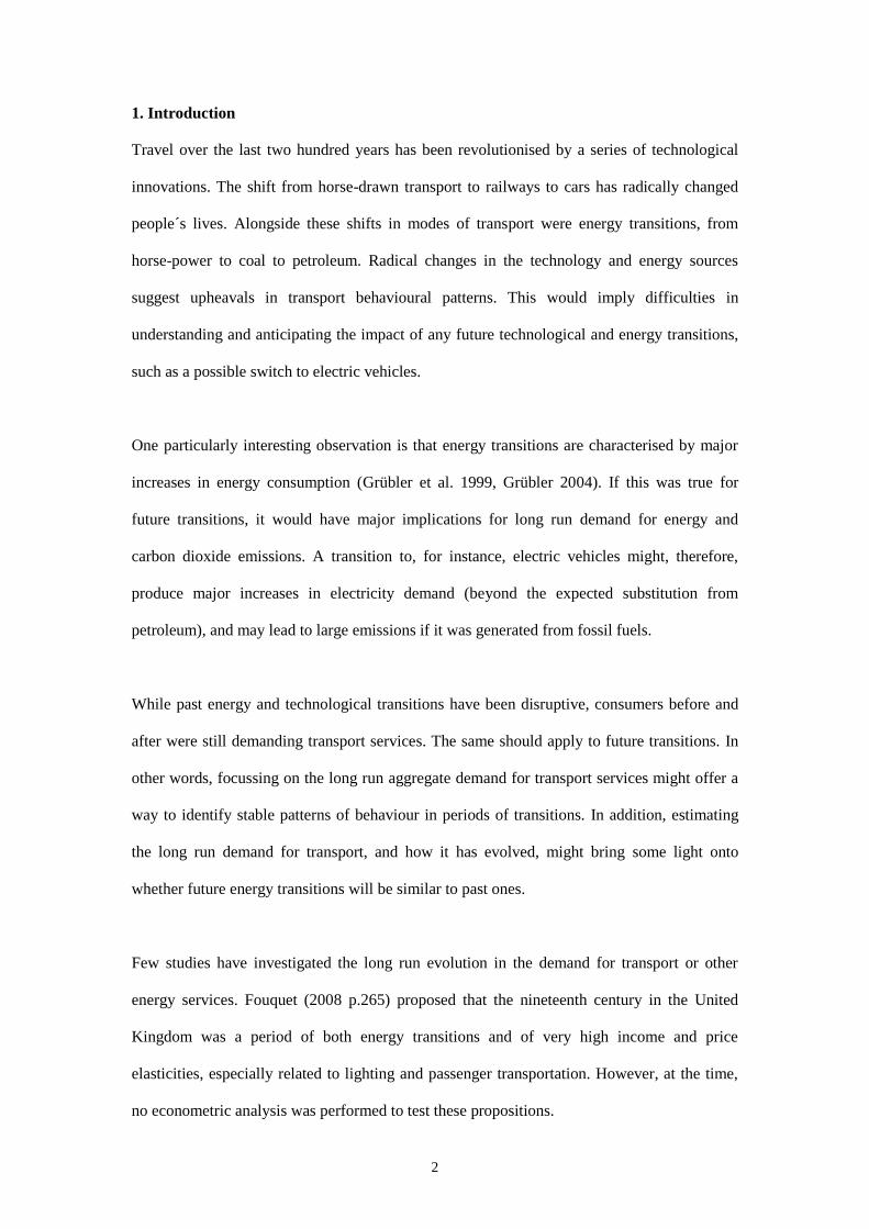
Abstract
The purpose of this paper is to estimate trends in income and price elasticities and to offer
insights for the future growth in transport use, with particular emphasis on the impact of
energy and technological transitions. The results indicate that income and price elasticities of
passenger transport demand in the United Kingdom were very large (3.1 and -1.5,
respectively) in the mid-nineteenth century, and declined since then. In 2010, long run income
and price elasticity of aggregate land transport demand were estimated to be 0.8 and -0.6.
These trends suggest that future elasticities related to transport demand in developed
economies may decline very gradually and, in developing economies, where elasticities are
often larger, they will probably decline more rapidly as the economies develop. Because of
the declining trends in elasticities, future energy and technological transitions are not likely
to generate the growth rates in energy consumption that occurred following transitions in the
nineteenth century. Nevertheless, energy and technological transitions, such as the car and
the airplane, appear to have delayed and probably will delay declining trends in income and
price elasticity of aggregate land transport demand.
Keywords: Income and Price Elasticities of Demand for Transport; Energy Transitions;
Rebound Effects
Published as: Fouquet, R. (2012) ‘Trends in income and price elasticities of transport demand (1850-
2010).’ Energy Policy 50: 50-61.
2
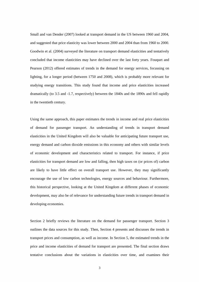
1. Introduction
Travel over the last two hundred years has been revolutionised by a series of technological
innovations. The shift from horse-drawn transport to railways to cars has radically changed
people´s lives. Alongside these shifts in modes of transport were energy transitions, from
horse-power to coal to petroleum. Radical changes in the technology and energy sources
suggest upheavals in transport behavioural patterns. This would imply difficulties in
understanding and anticipating the impact of any future technological and energy transitions,
such as a possible switch to electric vehicles.
One particularly interesting observation is that energy transitions are characterised by major
increases in energy consumption (Grübler et al. 1999, Grübler 2004). If this was true for
future transitions, it would have major implications for long run demand for energy and
carbon dioxide emissions. A transition to, for instance, electric vehicles might, therefore,
produce major increases in electricity demand (beyond the expected substitution from
petroleum), and may lead to large emissions if it was generated from fossil fuels.
While past energy and technological transitions have been disruptive, consumers before and
after were still demanding transport services. The same should apply to future transitions. In
other words, focussing on the long run aggregate demand for transport services might offer a
way to identify stable patterns of behaviour in periods of transitions. In addition, estimating
the long run demand for transport, and how it has evolved, might bring some light onto
whether future energy transitions will be similar to past ones.
Few studies have investigated the long run evolution in the demand for transport or other
energy services. Fouquet (2008 p.265) proposed that the nineteenth century in the United
Kingdom was a period of both energy transitions and of very high income and price
elasticities, especially related to lighting and passenger transportation. However, at the time,
no econometric analysis was performed to test these propositions.
3
Small and van Dender (2007) looked at transport demand in the US between 1960 and 2004,
and suggested that price elasticity was lower between 2000 and 2004 than from 1960 to 2000.
Goodwin et al. (2004) surveyed the literature on transport demand elasticities and tentatively
concluded that income elasticities may have declined over the last forty years. Fouquet and
Pearson (2012) offered estimates of trends in the demand for energy services, focussing on
lighting, for a longer period (between 1750 and 2008), which is probably more relevant for
studying energy transitions. This study found that income and price elasticities increased
dramatically (to 3.5 and -1.7, respectively) between the 1840s and the 1890s and fell rapidly
in the twentieth century.
Using the same approach, this paper estimates the trends in income and real price elasticities
of demand for passenger transport. An understanding of trends in transport demand
elasticities in the United Kingdom will also be valuable for anticipating future transport use,
energy demand and carbon dioxide emissions in this economy and others with similar levels
of economic development and characteristics related to transport. For instance, if price
elasticities for transport demand are low and falling, then high taxes on (or prices of) carbon
are likely to have little effect on overall transport use. However, they may significantly
encourage the use of low carbon technologies, energy sources and behaviour. Furthermore,
this historical perspective, looking at the United Kingdom at different phases of economic
development, may also be of relevance for understanding future trends in transport demand in
developing economies.
Section 2 briefly reviews the literature on the demand for passenger transport. Section 3
outlines the data sources for this study. Then, Section 4 presents and discusses the trends in
transport prices and consumption, as well as income. In Section 5, the estimated trends in the
price and income elasticities of demand for transport are presented. The final section draws
tentative conclusions about the variations in elasticities over time, and examines their
4
implications for our understanding of energy transitions, long run energy consumption and
climate policy.
2. Demand for Transport Services
The demand for passenger transport services reflects individuals´ willingness to pay for
travelling from one place to another. Before the nineteenth century, as well as having very
limited incomes, people had lifestyles that required little transport. Work was in or near the
home. People socialised with their family and neighbours. Yet, historically and across
cultures people´s travel distances have been bound by their monetary and time budgets
(Schäfer 2000). Greater income allowed individuals to spend more money on travel.
Similarly, new technologies and cheaper travel created an opportunity for the location of
work and lifestyles to change (Grübler et al 1999, Bannister 2011). Although some evidence
supports a constant relationship between income and travel demand (Schäfer and Victor
2000), this crucial issue in future energy use and carbon dioxide emissions deserves a deeper
look.
Consumer responsiveness to changes in prices and income has depended on a number of
factors. Income elasticities tend to reflect whether consumers perceived a particular good as a
“luxury” or as a necessity. For so-called “luxury” goods and services, consumption increased
more than proportionally as income rose (i.e., high income elasticity). Normal goods and
services (or necessities) were likely to have low elasticities (i.e., less than 1). In some cases,
they were seen as inferior goods and services, and consumption declined with greater income.
The traditional view is that, at low levels of economic development, most goods and services
have been luxuries relative to basic foods. So, as incomes rose, except for basic foods,
consumption for all goods and services increased more than proportionally. As income
increased further, saturation effects implied that consumption and expenditure of many
previously “luxury” goods and services grew less than income (Moneta and Chai 2010).
5
Evidence suggests that expenditure categories mostly associated with services have tended to
experience relatively lower levels of saturation. This is partly explained by the introduction of
higher quality services delaying the saturation effect. Consistent with this, there is some, but
limited, evidence of saturation for travel services (Moneta and Chai 2010). In other words, as
an economy develops and incomes rise, income elasticities associated with travel service
demand might be expected to fall, but not necessarily to zero.
Price elasticity can be broken-down into the income and substitution effects. The income
effect depends on the proportion of the individual’s budget spent on the service and whether
the individual tends to spend a greater proportion of the budget on the service as income rises.
The substitution effect indicates the tendency to switch towards the cheaper good or service.
The more substitutes available for a particular service the greater will be the substitution
effect.
When considering the aggregated market for passenger transport services, it is difficult to
identify clear substitutes. One could argue that communication, such as postal services, the
telegraph, the telephone and emails, has offered a partial substitute, by being able to transmit
messages from one person to another without needing people to travel. Thus, cheaper, faster
and better communication over the last two hundred years may have reduced the need for
certain types of travel (Selvanathan and Selvanathan 1994). At the same time, they (and
especially other forms of communication, such as newspapers, radio, television and the
internet) have probably increased people´s desire to travel more generally (Salomon 1985).
Even today, with emails, there still appears to be a relationship between distance and the
mode of communication used – for interactions with people living less than 5km, people still
often engage in face-to-face communication; for regional interactions, the phone is used
mostly; and for greater distances, the internet is the predominant choice (Mok et al. 2010).
6
It is important to distinguish between the overall market elasticity of demand for transport and
the demand facing individual modes of transport. Here, the focus is on the overall demand to
identify a continuous demand for travel over different modes, technologies and energy
sources. Most studies, however, focus on a particular mode of transport, rather than aggregate
demand. An early survey of the literature offers an insight into some of the elasticities that
might be expected by modes of transport (Oum et al. 1990, see also Oum et al.1992). For rail
travel, it identifies a wide range of price elasticities between -0.11 and -1.80. The variation is
explained in great part by the purpose and type of rail travel. Average peak intra-city travel
was -0.15 – that is, a 10% rise (or fall) in prices only reduced (or increased) consumption
1.5%. Whereas urban off-peak rail price elasticity was -1. Inter-city business travel was -0.8,
and average leisure rail travel was estimated to be -1.4. For off-peak car travel, price
elasticities ranged from -0.06 and -0.88 and, for peak journeys, estimates were between -0.12
and -0.49. Peak bus demand was inelastic (i.e., 0), while off-peak demand ranged from -1.08
and -1.54. Out of interest, the authors also found that the price elasticity of demand for air
travel ranged from -0.08 to -4.51, indicating, in some cases, great sensitivity to prices for this
more “luxury” form of transport. However, this study was unable to distinguish between short
run and long run estimates. Also, these estimates are for developed economies, while the
current paper is interested in demand at different phases of economic development.
More recently, Goodwin et al. (2004) surveyed the literature associated with car travel. In
addition to providing a valuable range of estimates, they were interested in changes in
elasticities. Although their results depend on the assumptions made about a traveller´s utility
function, their theoretical expectations (presented in Hanly et al. 2002) were that price
elasticities increased when (fuel) prices were high and fell with lower prices, and that price
elasticities fell with income (and, thus, over time). One might also expect a decline in price
elasticities because, for certain journeys, transport and leisure are consumed jointly and the
travel costs becomes a declining share of the total costs. However, they found no clear
support for these expectations. On the other hand, they proposed that, because of saturation
7
effects, income elasticities might be expected to fall, and tentatively concluded that income
elasticities did fall.
Price elasticity is also of great interest to energy economists because of possible rebound
effects (Howarth 1997, Greening et al. 2000, Sorrell 2007). Jevons (1865) introduced the
concept of the rebound effect, arguing that improvements in energy efficiency were likely to
lead to greater energy consumption (not less). Ayres (2005) proposed that rebound effects for
‘macro’ innovations (i.e. radical innovations, like the steam engine) might generate large
rebound effects and increases in energy consumption; and ‘micro’ innovations that improve
the efficiency of existing technologies result in smaller rebound effects. Fouquet (2008 p.277)
proposed a few historical cases in the United Kingdom (particularly, freight transport between
1715 and the 1930s, passenger transport from the 1840s to the 1920s, and lighting during the
nineteenth century – the latter confirmed in Fouquet and Pearson (2012)) where the rebound
effects were very high – partially supporting Jevons’ (1865) hypothesis.
In this light, Small and van Dender (2007) examined the price elasticity of demand for car
transport. They looked at transport demand in the US between 1960 and 2004, and found that
price elasticities were lower between 2000 and 2004 than from 1960 to 2000. They suggest
that the rebound effect fell from 2.1% to 0.57% for a 10% efficiency improvement. Thus, for
this limited sample, efficiency improvements generated only minor increases in car travel and
considerable reductions in energy use. Hughes et al. (2006) also find that the price elasticity
of gasoline demand has declined through time, but that, at any particular time, higher incomes
groups have higher price elasticities than lower income groups. The very limited evidence on
trends in income and price elasticity of demand for transport demand, and related rebound
effects, invites a more detailed time series study. The rest of this paper seeks to provide more
evidence.
8
3. Data Sources and Creation
To study the relationship between passenger transport use, income and prices, it is necessary
to gather statistical information on travel and the prices of travelling or energy sources
associated with the different modes. This section offers a summary of the sources and
methods used to produce annual estimates of prices (or costs) and use of horse drawn
transport (1850-1924), railways (1850-2010), buses (1904-2010) and cars (1904-2010) in
Great Britain and then, from the 1920s, the United Kingdom - more detail can be found in
Fouquet (2008).
For horse-drawn transport, Chartres & Trunbull (1983 p.71) presented estimates of passenger
miles per week for a number of years between 1715 and 1840. Thompson (1976) offered
detailed estimates of the number of horses associated with different activities (stagecoaches,
carriage, riding, as well as farm and trade), during the nineteenth and early twentieth century,
and particularly from 1851. These can be linked to the 1840 estimate by Chartres and
Turnbull (1983 p.71) to estimate the average number of passenger kilometres per horse used.
With this average, the number of horses used for transport can be used for calculating the
millions or billions of passenger-kilometres (bpk) from 1851 and 1924. While this was a
rough estimate, in the second half of the nineteenth century, horse transport was dwarfed by
railways use.
For prices, Jackman (1960) collected considerable information on the cost of stage coach
travel in the eighteenth and nineteenth centuries. When these were divided by the distance for
particular stage coach journeys, they produced estimates of the price per passenger-kilometre.
From estimates of several of the main journeys in England, an average price was estimated.
For railway use, Hawke (1970 p.47) offered data on millions of passenger miles and millions
of journeys travelled between 1840 and 1870. Mitchell (1988 p.545) also presented data on
millions of journeys travelled annually from 1842 until 1913. Thus, to calculate passenger-
9
kilometres after 1870, it was necessary to have estimates of the distance travelled during an
average journey. Munby (1978 pp.106–7) gave estimates of billions of passenger-kilometres
and the average length of train journeys between 1920 and 1970. So, the gap was only
between 1870 and 1920. Surprisingly, the calculation of the average length of a railway
journey in 1870 (from Hawke 1970) and in 1920 (from Munby 1978) are virtually identical,
and the distance travelled on the average railway journey was assumed to have remained
nearly constant over those fifty years. Mitchell’s (1988) passenger journey data was
multiplied by the average length of journeys to estimate passenger transport in billions of
passenger-kilometres (bpk) between 1870 and 1913. To complement Munby (1978), from
1938 to 2010, DoT (2002) and DfT (2011) presented direct estimates of passenger-km.
These can then also be used to estimate the price of railway passenger services. Mitchell
(1988 p.545) has railway passenger receipts (in £m) between 1843 and 1980. These figures
can be divided by estimates of total passenger-km travelled (discussed above) to suggest the
cost per passenger-km of using railways up to 1913. Munby (1978 pp.113–14) has direct
estimates of the price (in old pence per km) from 1920 to 1970. Between 1970 and 1980,
receipts were again divided by passenger-km. DoT (2002) and DfT (2011) had estimates of
the price between 1991 and 2010. An inability to find values during the 1980s led to
interpolation.
For twentieth century road travel, DoT (2002) and DfT (2010) presented data on passenger
travel (e.g., buses, cars, motorcycles, etc…) between 1952 and 2010. Before the early 1950s,
data needed to be pulled together. Mitchell (1988 pp.557–8) had information on the number
of cars and other vehicles between 1904 and 1980. Car passenger travel per vehicle was
calculated for 1952 - 16,000 km per car per year. Before these years, assumptions were made
about the trend in average travel per vehicle: for cars, an annual 2% decrease in the average
travel per car ratio each year before 1952 – based on the idea that there were fewer roads and
people travelled less per year than they did in the 1950s. This assumed trend in average
10
distance per vehicle (back to the beginning of the century) was multiplied by Mitchell’s (1988
pp.557–8) numbers of vehicles to produce an estimate of the bpk (billions of passenger
kilometres) back to 1904. Given that the number of buses was also available, a similar method
was used to quantify bpk used related to public transport vehicles (Fouquet 2008).
Passenger road transport ‘prices’ are more complex in the second-half of the twentieth
century. Rather than identifying the cost of buying a train or bus ticket, as more travellers
used their own cars, a number of different expenditures were involved. At least three costs
can be identified: the fuel costs, all marginal costs and annualized total costs. Table 1 shows
the breakdown of the annual cost of car travel between 1971 and 2008. Fuel costs accounted
for between 28%-40% of the total annual expenses. Few of the other expenses listed are
obvious marginal costs – tyre consumption also depends on distance travelled. So, fuel costs
were presented as the price (or main private marginal cost) of passenger transport.
The price of driving a car one kilometre was estimated by dividing passenger fuel expenditure
(in million tonnes of oil equivalent (mtoe)) by distance travelled (in bpk). Until the 1930s,
motor spirit (i.e., gasoline) was the main petroleum product for road vehicles. Then, diesel
(that is, ‘derv’) began to be used by goods vehicles and buses. Cars used exclusively motor
spirit until the 1980s, when diesel started to take a small market share. Thus, it was necessary
to identify the share of motor spirit and diesel consumed for passenger services.
The Ministry of Power (MoP 1961) indicated the share of motor spirit used by both passenger
and freight transport between 1938 and 1960. The share of motor spirit used by commercial
vehicles fell from 42% to 19% in that period – it was assumed that the share of buses was
around 10% of commercial vehicles in 1938 and 5% by 1960, reflecting the relative decline
of public transport. These shares enabled motor spirit consumption (DTI 2011 and back
copies, MoP 1961 and King 1952 p.551) to be estimated for passenger travel.
11
DTI (2011) presented the amount of diesel used by passenger travel back to 1995; in 2000, it
was equivalent to 18% of the total consumption of diesel. Miller (1993) indicated the share of
diesel vehicles in the passenger vehicle stock into the early 1990s, providing a basis for
calculating the small amount of diesel consumed. An interpolation connected 1991 and 1995.
The rest of road transport diesel (also found in DTI 1997, 2001, MoP 1961 and King 1952
p.551) was assumed to be for freight. Thus, consumption of motor spirit and derv for
passenger road transport were estimated between 1910 and 2000.
DTI (1997, 2001, 2011) presented the price of motor spirit and diesel back to 1954. The
Institute of Petroleum (1994) had data on the price of motor spirit from 1902 to 1953. The
prices were multiplied to the consumption estimates to calculate the fuel expenditure of
passenger road transport. Dividing fuel expenditure by distance enabled an estimate of fuel
costs of road transport services in pence per passenger-km. All prices for transport service
were converted into real terms using the data available in Allen (2007).
4. Trends in Transport Prices and Use
Passenger transport in Britain experienced a series of revolutions that radically altered the
ability to travel. First, from the mid-seventeenth century, the introduction of turnpikes,
managed roads that travellers paid to use, enabled an improved road network. Then, from the
1770s, stage coach journeys became better managed and faster – by 1830, average trips took
one-fifth of the time they took in the 1770s (Bagwell 1974). Between 1775 and 1815,
passenger travel increased from 0.05 billion passenger-km (bpk) to 3 bpk – a sixty-fold
increase in fifty years (Chartres and Turnbull 1983).
Then, harnessing the power of steam by heating fuels revolutionised the economy and society.
It, first, provided stationary power to remove water from coal mines and to spin cotton, then,
as directed power, enabled transport along railways (and for ships). The introduction of steam
12
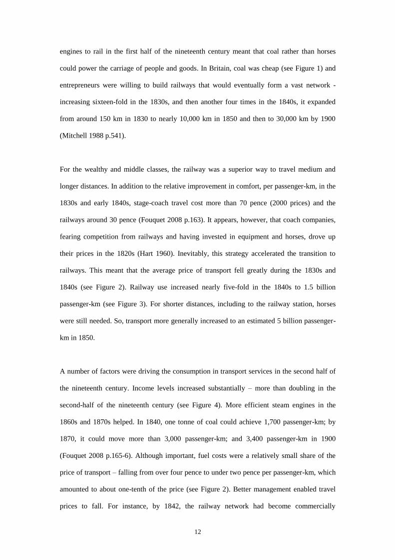
engines to rail in the first half of the nineteenth century meant that coal rather than horses
could power the carriage of people and goods. In Britain, coal was cheap (see Figure 1) and
entrepreneurs were willing to build railways that would eventually form a vast network -
increasing sixteen-fold in the 1830s, and then another four times in the 1840s, it expanded
from around 150 km in 1830 to nearly 10,000 km in 1850 and then to 30,000 km by 1900
(Mitchell 1988 p.541).
For the wealthy and middle classes, the railway was a superior way to travel medium and
longer distances. In addition to the relative improvement in comfort, per passenger-km, in the
1830s and early 1840s, stage-coach travel cost more than 70 pence (2000 prices) and the
railways around 30 pence (Fouquet 2008 p.163). It appears, however, that coach companies,
fearing competition from railways and having invested in equipment and horses, drove up
their prices in the 1820s (Hart 1960). Inevitably, this strategy accelerated the transition to
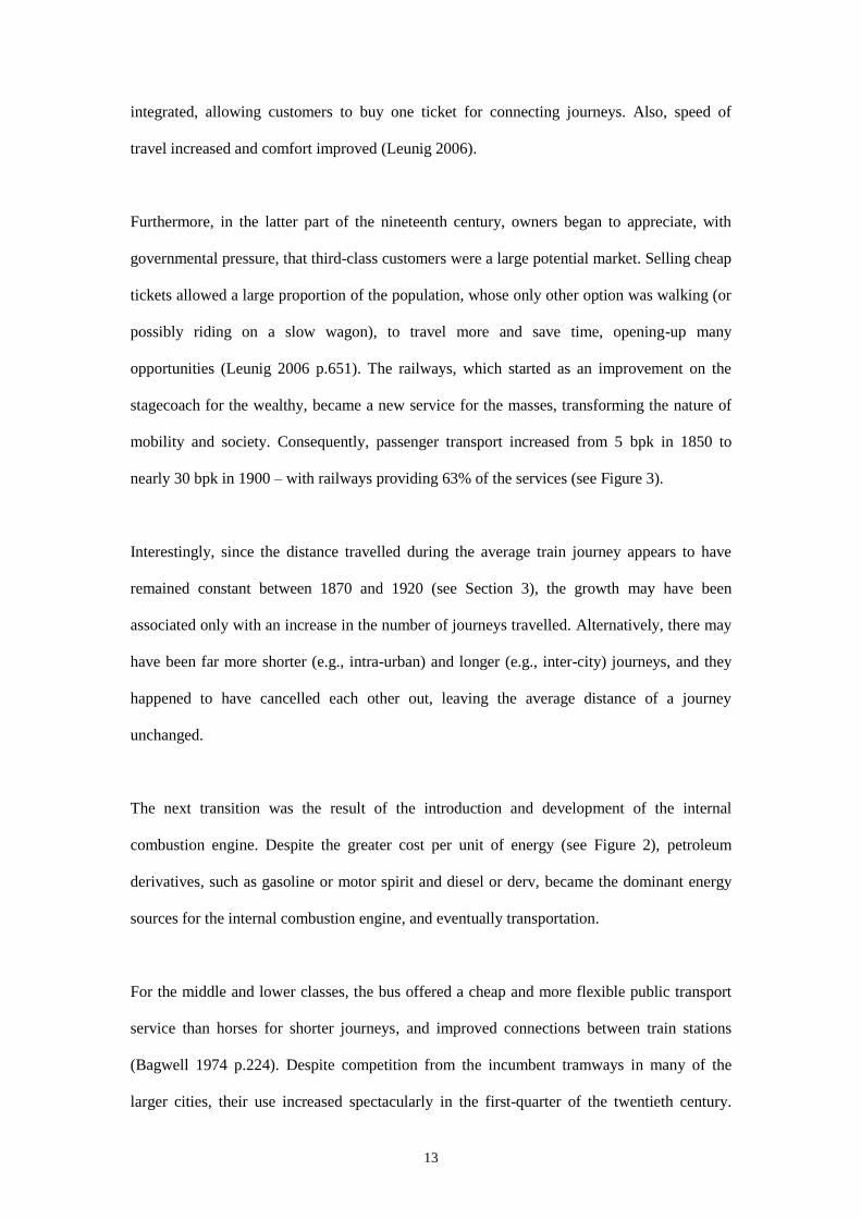
railways. This meant that the average price of transport fell greatly during the 1830s and
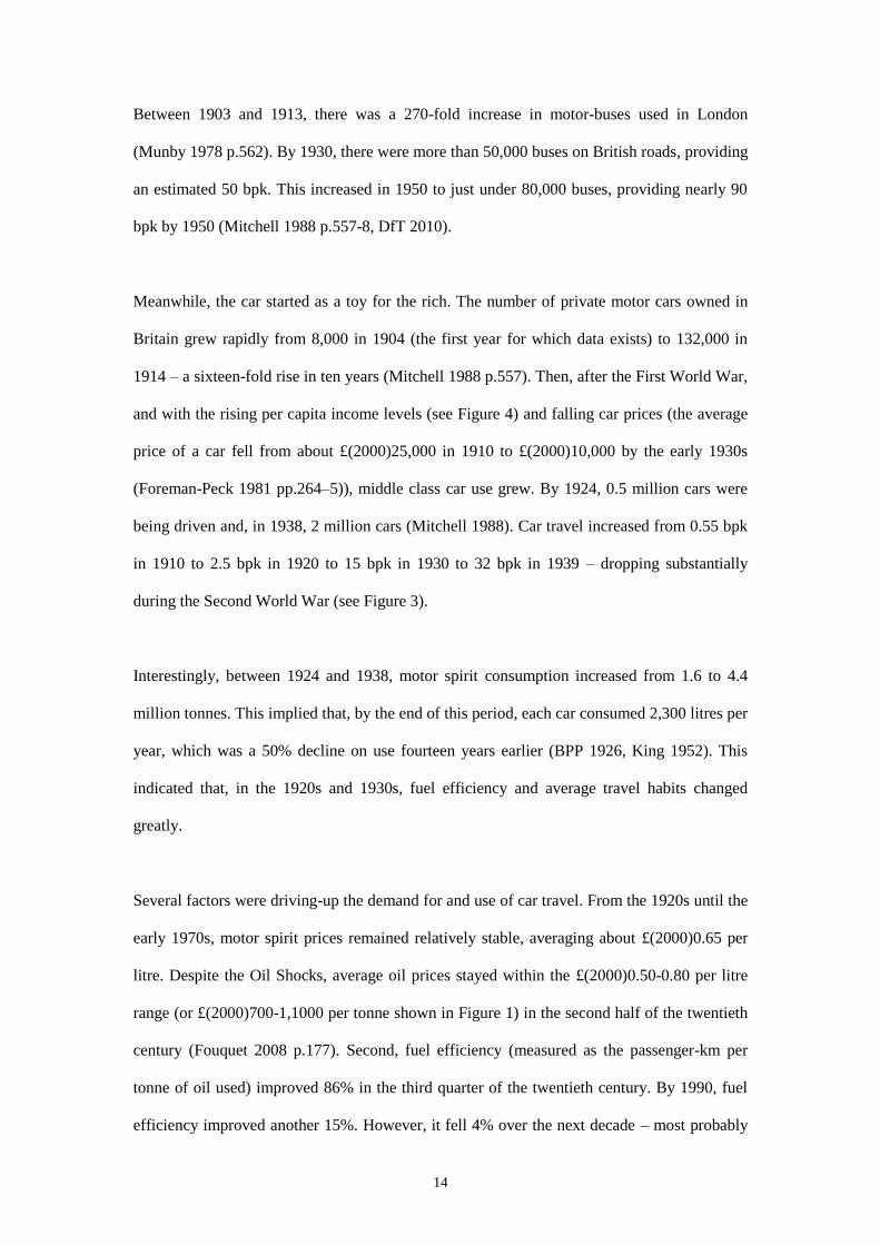
1840s (see Figure 2). Railway use increased nearly five-fold in the 1840s to 1.5 billion
passenger-km (see Figure 3). For shorter distances, including to the railway station, horses
were still needed. So, transport more generally increased to an estimated 5 billion passenger-
km in 1850.
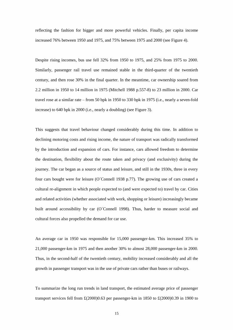
A number of factors were driving the consumption in transport services in the second half of
the nineteenth century. Income levels increased substantially – more than doubling in the
second-half of the nineteenth century (see Figure 4). More efficient steam engines in the
1860s and 1870s helped. In 1840, one tonne of coal could achieve 1,700 passenger-km; by
1870, it could move more than 3,000 passenger-km; and 3,400 passenger-km in 1900
(Fouquet 2008 p.165-6). Although important, fuel costs were a relatively small share of the
price of transport – falling from over four pence to under two pence per passenger-km, which
amounted to about one-tenth of the price (see Figure 2). Better management enabled travel
prices to fall. For instance, by 1842, the railway network had become commercially
13
integrated, allowing customers to buy one ticket for connecting journeys. Also, speed of
travel increased and comfort improved (Leunig 2006).
Furthermore, in the latter part of the nineteenth century, owners began to appreciate, with
governmental pressure, that third-class customers were a large potential market. Selling cheap
tickets allowed a large proportion of the population, whose only other option was walking (or
possibly riding on a slow wagon), to travel more and save time, opening-up many
opportunities (Leunig 2006 p.651). The railways, which started as an improvement on the
stagecoach for the wealthy, became a new service for the masses, transforming the nature of
mobility and society. Consequently, passenger transport increased from 5 bpk in 1850 to
nearly 30 bpk in 1900 – with railways providing 63% of the services (see Figure 3).
Interestingly, since the distance travelled during the average train journey appears to have
remained constant between 1870 and 1920 (see Section 3), the growth may have been
associated only with an increase in the number of journeys travelled. Alternatively, there may
have been far more shorter (e.g., intra-urban) and longer (e.g., inter-city) journeys, and they
happened to have cancelled each other out, leaving the average distance of a journey
unchanged.
The next transition was the result of the introduction and development of the internal
combustion engine. Despite the greater cost per unit of energy (see Figure 2), petroleum
derivatives, such as gasoline or motor spirit and diesel or derv, became the dominant energy
sources for the internal combustion engine, and eventually transportation.
For the middle and lower classes, the bus offered a cheap and more flexible public transport
service than horses for shorter journeys, and improved connections between train stations
(Bagwell 1974 p.224). Despite competition from the incumbent tramways in many of the
larger cities, their use increased spectacularly in the first-quarter of the twentieth century.
14
Between 1903 and 1913, there was a 270-fold increase in motor-buses used in London
(Munby 1978 p.562). By 1930, there were more than 50,000 buses on British roads, providing
an estimated 50 bpk. This increased in 1950 to just under 80,000 buses, providing nearly 90
bpk by 1950 (Mitchell 1988 p.557-8, DfT 2010).
Meanwhile, the car started as a toy for the rich. The number of private motor cars owned in
Britain grew rapidly from 8,000 in 1904 (the first year for which data exists) to 132,000 in
1914 – a sixteen-fold rise in ten years (Mitchell 1988 p.557). Then, after the First World War,
and with the rising per capita income levels (see Figure 4) and falling car prices (the average
price of a car fell from about £(2000)25,000 in 1910 to £(2000)10,000 by the early 1930s
(Foreman-Peck 1981 pp.264–5)), middle class car use grew. By 1924, 0.5 million cars were
being driven and, in 1938, 2 million cars (Mitchell 1988). Car travel increased from 0.55 bpk
in 1910 to 2.5 bpk in 1920 to 15 bpk in 1930 to 32 bpk in 1939 – dropping substantially
during the Second World War (see Figure 3).
Interestingly, between 1924 and 1938, motor spirit consumption increased from 1.6 to 4.4
million tonnes. This implied that, by the end of this period, each car consumed 2,300 litres per
year, which was a 50% decline on use fourteen years earlier (BPP 1926, King 1952). This
indicated that, in the 1920s and 1930s, fuel efficiency and average travel habits changed
greatly.
Several factors were driving-up the demand for and use of car travel. From the 1920s until the
early 1970s, motor spirit prices remained relatively stable, averaging about £(2000)0.65 per
litre. Despite the Oil Shocks, average oil prices stayed within the £(2000)0.50-0.80 per litre
range (or £(2000)700-1,1000 per tonne shown in Figure 1) in the second half of the twentieth
century (Fouquet 2008 p.177). Second, fuel efficiency (measured as the passenger-km per
tonne of oil used) improved 86% in the third quarter of the twentieth century. By 1990, fuel
efficiency improved another 15%. However, it fell 4% over the next decade – most probably
15
reflecting the fashion for bigger and more powerful vehicles. Finally, per capita income
increased 76% between 1950 and 1975, and 75% between 1975 and 2000 (see Figure 4).
Despite rising incomes, bus use fell 32% from 1950 to 1975, and 25% from 1975 to 2000.
Similarly, passenger rail travel use remained stable in the third-quarter of the twentieth
century, and then rose 30% in the final quarter. In the meantime, car ownership soared from
2.2 million in 1950 to 14 million in 1975 (Mitchell 1988 p.557-8) to 23 million in 2000. Car
travel rose at a similar rate – from 50 bpk in 1950 to 330 bpk in 1975 (i.e., nearly a seven-fold
increase) to 640 bpk in 2000 (i.e., nearly a doubling) (see Figure 3).
This suggests that travel behaviour changed considerably during this time. In addition to
declining motoring costs and rising income, the nature of transport was radically transformed
by the introduction and expansion of cars. For instance, cars allowed freedom to determine
the destination, flexibility about the route taken and privacy (and exclusivity) during the
journey. The car began as a source of status and leisure, and still in the 1930s, three in every
four cars bought were for leisure (O´Connell 1938 p.77). The growing use of cars created a
cultural re-alignment in which people expected to (and were expected to) travel by car. Cities
and related activities (whether associated with work, shopping or leisure) increasingly became
built around accessibility by car (O´Connell 1998). Thus, harder to measure social and
cultural forces also propelled the demand for car use.
An average car in 1950 was responsible for 15,000 passenger-km. This increased 35% to
21,000 passenger-km in 1975 and then another 30% to almost 28,000 passenger-km in 2000.
Thus, in the second-half of the twentieth century, mobility increased considerably and all the
growth in passenger transport was in the use of private cars rather than buses or railways.
To summarize the long run trends in land transport, the estimated average price of passenger
transport services fell from £(2000)0.63 per passenger-km in 1850 to £(2000)0.39 in 1900 to
16
£(2000)0.08 in 1950 to £(2000)0.05 in 2000 – a twelve-fold decline in 150 years. Income per
capita increased from £(2000)1,500 per year in 1850 to £(2000)3,200 in 1900 to £(2000)5,200
in 1950 to £(2000)17,000 in 2000 – nearly a twelve-fold rise in 150 years. Land passenger
transport consumption soared from less than 4.5 bpk in 1850 to 27 bpk in 1900 to 186 bpk in
1950 to nearly 740 bpk in 2000 – a 165-fold rise in 150 years. If income and price were both
unit elastic in relation to transport demand for these 150 years, consumption would have
increased 144-fold. Thus, the evidence suggests the demand for land transport was either
elastic for the last 150 years or very elastic during certain periods.
Yet, the introduction of air travel has increased total passenger transport even more rapidly
over the last sixty years. In 1950, airplanes provided 2 bpk. By 1975, this had increased to 62
bpk, and up to 260 bpk in 2000, reaching 305 bpk in 2010. So, at present, air travel provides
almost half the number of passenger kilometres that cars do – airplanes are responsible for
28% of all passenger transport and cars for 61%. Recent total1 (i.e., land and air) use
increased more - from 192 bpk in 1950 to 1,012 bpk in 2000, and 1,095 bpk in 2010. Thus,
total passenger transport increased 220-fold in 150 years, indicating even higher income
and/or price elasticities.
5. Income and Price Elasticities, and Rebound Effects
This section presents some estimates of the influence of income and prices on transport use,
and their trends over the last 150 years. Following the same approach as Fouquet and Pearson
(2012), a vector error correcting model was used to provide an econometric analysis of the
data and the trends, and estimate the cointegrated relationship between travel, income and
1 Sea passenger transport was excluded because the author has only managed to find data from 1950,
despite its historical role in international transport. In 1950, there were 6.4 bpk by sea, implying that it
provided less than 4% of total passenger travel at the time. Its role fell further, providing less than 3
bpk at the beginning of the twenty-first century (DfT 2011).
17
transport prices. The emphasis should not be on the methods used, which are open to criticism
and other scholars might improve upon2, but the trends.
Given the trended nature of the data (see Figures 2, 3 and 4) and the tendency for long run
transport use (or energy related to transport), GDP and travel costs to be cointegrated
(Bentzen 1994, Fouquet 1997, Ramanathan 1999), the possibility of using vector error-
correcting models (VECM) was explored. From a statistical perspective, such models were
appropriate.
First, for the long run trends in transport consumption, GDP per capita and the price of
transport, non-stationarity could not be rejected. In addition to the standard tests for unit roots,
an augmented Dickey-Fuller test where the time series is transformed via a generalized least
squares (GLS) regression was used to improve the power of the test (Elliott, Rothenberg and
Stock 1996). Here, for up to 15 lags, and incorporating the assumption of a time trend, the
tau-statistics could not reject at the 10% confidence level. Thus, unit roots (i.e. non-
stationarity) were likely.
Second, the causal relationship between transport consumption and per capita GDP was
examined. The results suggest unidirectional causality from per capita GDP to transport use.
As expected, GDP per capita was not influenced by either transport use or prices, as transport
has been only a small component of economic activity (generally less than 8% of GDP).
Although still significant, as will be shown by certain elasticity estimates, the causality test
indicated that prices were less of a powerful explanatory variable of transport consumption.
The results indicate that, in the second-half of the nineteenth century, consumption may have
also influenced prices – perhaps reflecting the importance of economies of scale in driving
2 The author would like to thank Bill Nordhaus, David Stern, Lester Hunt and Lutz Killian for their
comments on this avenue of research. Lutz Killian questioned whether long run elasticities can be
estimated with time series, rather than with panel data (See Killian and Murphy 2009). The other three
18
down early railway costs. While this raised a simultaneity problem, for this exercise, it was
assumed that causality was unidirectional from prices to consumption for the whole period.
Third, tests rejected the null hypothesis of no cointegrating equations for the relationship
between transport consumption, GDP per capita and the price of transport – for the whole
period between 1850 and 2010 (see below). Having selected the appropriate number of lags
from a series of different tests (Nielson 2001), tests for the existence of cointegrating
equations were performed and, when the null hypothesis of no relationship was rejected,
almost always one cointegrated relationship could not be rejected (based on methods
developed in Johansen 1988, 1995).
These VECM were, therefore, used to estimate the evolution of income and price elasticities.
The approach was to estimate elasticities for fifty year periods moving through time. For
example, the income and price elasticities were estimated for the period 1850-1899, then
1851-1900, and so on until 1961-2010. Then, the elasticity for any particular year would be
the moving average (i.e., the average of all elasticities estimated where that year was
included). For example, for the moving average around the year 1950, fifty income elasticity
estimates were produced (for the periods 1900-1950, 1901-1951, and so on until 1950-2000)
and the average of all these estimates was equal to 0.91. Estimated in the same way, the
average price elasticity around 1950 was -0.72.
Inevitably, for some periods, the results were either not as expected or the possibility of no
cointegrated relationship could not be rejected. In particular, the period broadly between 1850
and 1869 produced unexpected price elasticities and the absence of cointegrating relationships
could not be rejected. Most of the price elasticities were positive and large. In the absence of a
satisfactory explanation, these estimates were excluded from the calculation of the average
scholars encouraged this line of research, although offered caution about the methods. Naturally, the
author of this paper is solely responsible for the choices made and the limitations of the methods used.
19
estimates. Consequently, for the years 1850-1869 less than five estimates for price elasticity
were available and no average was calculated. Nevertheless, the majority of estimates
produced standard signs and sizes – income elasticity estimates were used for 97% of the
moving averages over the 160 years and, between 1870 and 2010, price elasticity estimates
for 93% of the moving averages.
Figure 5 presents the trends. It shows the clear the decline (in absolute terms) of both income
and price elasticities. In the third quarter of the nineteenth century, they were at their highest,
falling in several waves, the first, in the final quarter of the century, then, in the early 1900s,
and, finally, from the 1920s until the end of the century, a gradual decline for land transport.
It is worth noting first, however, that consumption associated with horse-drawn carriage in the
late eighteenth and early nineteenth centuries had increased 60-fold in fifty years (Chartres
and Turnbull 1983). In the last quarter of the eighteenth century, average income grew 30%,
travel prices fell around 25% and journey speeds increased up to 80%. Thus, although there is
a lack of annual data, it indicates spectacular sensitivity to changes in availability, prices,
quality of service and income levels. So, we can conclude that income (and other variable)
elasticities were very high, especially in the late 1700s.
In the 1850s, income elasticity was also very high - a 10% increase in income led to a 31%
increase in travel (see Table 2). The creation and expansion of the railway network allowed
the upper and growing middle classes to travel more. This expansion coincided with the rise
in average income levels during the mid-nineteenth century. Transport services were a key
household expenditure. During the second-half of the nineteenth century, expenditure as a
proportion of GDP increased from 6% to 7% (Fouquet 2008 p.271). At the time, households
were spending three times more on travelling than on heating their homes and six times more
than on lighting their homes.
20
The growth in average income throughout the nineteenth century, as well as the decline in
prices, made railways accessible not only to upper and middle classes, but also working
classes. Fouquet and Pearson (2012), commenting about lighting demand, proposed that
below certain levels of accessibility, the energy service only provides a basic level of service.
However, beyond a threshold, the service can help to meet many other demands – in relation
to work and to leisure, thus, transforming lives.
For instance, the expansion of the railways coincided with increased urbanisation. As
populations moved to urban centres from the beginning of the nineteenth century, they were
closer to transport nodes, thus, more able to take advantage of transport services. Later, in the
second-half of the nineteenth century, the expansion of suburbia was driven by the growth in
suburban railway services. From the 1840s, upper and upper-middle class households had
sought to move away from the crime, sewage and smoke, and the expansion of urban railway
networks enabled them to move to the suburbs (Luckin 2000). The introduction of the Cheap
Trains Act of 1883 and a rapid expansion of suburban housing in the 1890s offered an
opportunity for lower-middle class families to live in the suburbs and commute into the city
(Jackson 2003, Burnett 1986). The urbanised area of London increased five-fold between
1841 and 1901 (Demographia 2011). Thus, transport changed people´s lifestyles, which, in
turn, required higher levels of transport services to be sustained.
While transport services were still a “luxury”, by the early 1900s, income elasticity of
transport demand fell dramatically. It fell from an average of 2.2 in the 1890s to 1.2 in the
1920s (see Table 2). Surprisingly, the development of the internal combustion engine and the
growth of bus and car use did not stop the decline in income elasticity. After the Second
World War, land transport became a “necessity”, as it was an essential part of everyday life.
It is surprising that the introduction of cars, allowing for personal freedom of travel and
privacy, did not raise income elasticity. Nevertheless, without the introduction of cars, income
21
elasticity of travel demand would probably have fallen further, implying a substantially less
mobile economy and society. In other words, the technological and energy transition
associated with the internal combustion engine and particularly the car, which offered a
different travelling experience, probably slowed the decline in income elasticities.
This hypothesis (that energy and technological transitions can delay the decline in income
elasticities) is supported for air travel. When the same regressions were run using total (land
and air) passenger transport, income elasticity stayed around 1.2 between the 1920s and 1980s
(see Table 2 and Figure 5). Nevertheless, looking in a little more details indicates that income
elasticities for total passenger transport started to decline from the mid-1960s, but only
reached unity at the beginning of the twenty-first century. For land passenger transport, an
income elasticity of 1 was reached in the 1940s. Thus, it appears that the introduction of air
travel delayed the decline in passenger transport income elasticity by roughly sixty years.
Interestingly, air travel had far less influence over price elasticities. It very slightly reduced
consumer sensitivity to prices. This may be because consumers are more driven by their rising
incomes. More probably, however, it simply reflects the price variable used. This was an
average of land passenger transport, and does not incorporate the declining price of air travel
between 1950 and 2010, for which data was not found.
Returning to the long run trends, the general decline in land transport price elasticities was
more gradual than for income (see Table 2). In the 1870s, price elasticity was -1.5, implying
that a 10% decrease in transport prices would lead to a 15% rise in passenger travel (during
the 1850s and 1860s, only a few of the price elasticity estimates were significant). This fell
close to -1 by 1890, falling to -0.9 during the 1920s and to -0.7 for most of the second-half of
the twentieth century. Between 2000 and 2010, price elasticity stood at -0.6. This indicates
that, over the last 60 years (and throughout the major shift to cars, the dependence on oil for
22
transport and the Oil Shocks), a surprisingly stable relationship has existed between transport
(and indirectly petrol) prices and consumption.
Separating price elasticity into its two components can help a little to understand the decline.
The income effects appear to have fallen – travel expenditure relative to GDP fell from more
than 8% in the 1920s down to 2% at the end of the twentieth century (Fouquet 20008 p.271).
So, changes in prices would have had a much greater effect on consumer purchasing power at
the beginning of the twentieth century than at the beginning of the twenty-first century. Given
the difficulty of identifying clear substitutes for transportation, it is hard to assess whether the
substitution effect changed over the last 150 years. It is possible that communication
technologies could have acted as a substitute for certain transport needs. However, the
telephone, for instance, was very slow to diffuse in the United Kingdom – although
introduced in 1881, only 21% of households had telephones by 1965; this increased to 77% in
1983 (Bowden and Offer 1994 p.744). One might propose that, during the twentieth century,
while income effects were falling, the substitution potential was increasing. Thus, the
considerable changes in income effects and possibly substitution effects over the last 80 years
may have cancelled each other out (to a certain extent), implying that there was only a modest
decline in price elasticities.
Transport demand price elasticities are also of interest for identifying possible rebound
effects. Energy efficiency improvements associated with cars effectively reduced the marginal
cost of travel. Although this was not very relevant for the nineteenth century, since the fuel
costs were a small proportion of the price of rail transport, it has been more important in the
second-half of the twentieth century or the twenty-first century. The study suggests that,
despite the Oil Shocks and major changes in car technology, consumers today may still be
increasing their travel by 6% for a 10% increase in fuel efficiency, implying only a 4% energy
saving. That is, this study proposes that there is a substantial rebound effect associated with
aggregate transport demand.
23
This is considerably larger than other studies, such as Small and van Dender (2007). One
explanation is that, in fact, the rebound effect will be smaller than 6%, because fuel costs (if
one of the main marginal costs) tend to be less than one-third (although 40% in 2008) of the
total annual expenditure on cars (see Table 1). So, the rebound effect may be considerably
lower – that is, closer to 2%, implying a 8% energy saving. Another possible explanation is
that studies that focus only on car travel will tend to ignore the effects between modes of
transport – such as cheaper costs of running a car encourage rail users to travel more by car.
6. Conclusion
This paper sought to estimate the trends in real income and price elasticities of demand for
aggregate transport. Focussing on the experience in the United Kngdom, it tried to identify
the influences of the increase in per capita income (12-fold between 1850 and 2000) and of
the decline in the real price of transport (12-fold between 1850 and 2000) on the rapid rise in
aggregate passenger land transport consumption (165-fold over 150 years). Using standard
econometric techniques and modelling of long run economic behaviour, a series of income
and price elasticities were estimated. For each year, a moving average estimate was
calculated, thus, providing a time series of the income and price elasticities from the middle
of the nineteenth century to the beginning of the twenty-first century.
The results indicate that income and price elasticities were very large (3.1 and -1.5,
respectively) in the mid-nineteenth century and declined continuously since then. Land
transport demand became price inelastic (i.e., less than one) in the early 1920s and income
inelastic at the end of the 1930s and in the early 1940s. However, the trends in income
elasticity for total passenger transport demand remained higher, around 1.2, and only fell to
unity in the twenty-first century. This indicated that the introduction of air travel delayed the
decline in income elasticities by sixty years.
24
It is worth stressing points made earlier about the study´s limitations. The reliability and
coverage of the data (especially for the nineteenth century) and also the validity of the
econometric procedures can be questioned and criticised. Perhaps the estimates are the
outcome of a flawed statistical analysis. Yet, the econometric estimates broadly match the
data – that is, between 1850 and 1900, jointly income and price elasticities were greater than
one and, between 1950 and 2000, for land transport, they were less than one.
Also, providing a long-run perspective on changes in transport demand elastiticies, these
results support theoretical and prior empirical expectations about transport demand. These
expectations were, first, that saturation effects will reduce income elasticity, although more
slowly than for basic goods (Hanly et al. 2002, Moneta and Chai 2010, Goodwin et al. 2004)
and, second, that price elasticities fall as prices decline and incomes rise (Hanly et al. 2002,
Small and van der Dender 2007). They are also similar to the trends in elasticities for lighting
demand – income and price elasticities peaked in the second-half of the nineteenth century
(3.5 and -1.7, respectively) and declined during the twentieth century (Fouquet and Pearson
2012).
As well as matching expectations and providing greater detail on trends, these results are of
interest for anticipating future behaviour. The elasticity estimates, which were remarkably
stable during the twentieth century, suggest that aggregate passenger land transport
consumption in the United Kingdom will increase by 8% from a 10% rise in income and by
6% from a 10% decline in average transport prices in the early twenty-first century. This also
gives clues to the rebound effect, which is estimated to be between 2% and 6% from a 10%
fuel efficiency improvement.
Since the study offers a long run perspective, some readers may be interested in long run
forecasts of trends in elasticities. It is obvious that to do so is to risk being very wrong.
25
However, current forecasts of energy demand and carbon emissions look forward decades and
centuries, and depend on some evidence about the trends in elasticities. So, despite the
speculative nature of forecasting (and the slight increase in income elasticities during the first
decade of the twenty-first century), the trends in this study and prior expectations suggest that
income and price elasticities are likely to decline gradually.
One of the reasons for focusing on aggregate transport demand and the related elasticity
trends was to identify the impact of energy transitions on energy use. Aggregate transport
demand offered a stable variable through periods of dramatic change. It is important to point-
out that, within this framework, energy and related technological transitions have two ways to
influence aggregate transport demand (Fouquet 2010): first, by reducing the costs or prices of
transport services, which did occur in past transitions, and can be represented by a slide down
the demand curve; and, second, through providing higher quality services, which also
occurred, and might be reflected by a shift in the demand curve.
Here, it is proposed that the dramatic increase in energy consumption that followed the
transition from stage coaches (and horse power) to railways (and coal) was due to very high
income and price elasticities. Prices fell substantially generating greater transport use. Even
more important seems to have been the dramatic shift in the demand curve (reflected in the
high income elasticity). The transition to the internal combustion engine (and petroleum
products), buses and cars, led to a large increase in energy consumption. However, income
elasticities were around unity and price elasticities were less than one. In other words, the
energy transition from coal to petroleum boosted energy consumption relatively less than the
one from horse power to coal. Given past trends, prior expectations and the tentative forecast
above, it is tempting to conclude that any future energy transition in the land transport sector
will increase energy consumption relatively less than past transitions.
26
Having said this, the demand for transport-related energy is driven first by the demand for
transport and then by the relationship between the technology for providing transport and the
amount of energy required (Small and van Dender 2007). The extent of the increase in energy
consumption will depend on (i) the decline in transport prices, (ii) transport price elasticities,
(iii) the change in fuel efficiency, (iv) transport income elasticity and (v) improvements in the
quality of the transport service associated with the transition, which will affect the income
elasticity. The latter highlights an important feature of energy transitions: by raising the
quality of the service, as cars and arguably planes did, they delay the decline in elasticities.
So, when comparing two scenarios of the future (one with and one without transition), unless
the transition is towards a highly energy efficient technology (and this is possible), it is likely
that the scenario with an energy transition will generate higher energy consumption. Whether
this scenario produces more or less carbon dioxide emissions will depend on the energy
source used.
Up to this point, the discussion has been about behaviour in the United Kingdom, and
possibly by analogy in other developed economies. Since this study looks at trends in
elasticities at different phases of economic development, it can provide some clues to trends
in developing economies. Their elasticities are probably higher than in developed economies.
So, as these economies develop and incomes rise, transport use is likely to rise more than
proportionally, with major effects on the demand for current energy sources and on the local
and global environment.
It is possible that income and price elasticities are not as high in developing economies today
as in Victorian Britain – for a given level of income, transport prices are substantially lower in
developing economies today than in nineteenth century England. Also, as these economies
develop, their elasticities will probably also fall. Again, the introduction of new and superior
quality transport services associated with a transition will probably delay or slow-down the
declining trend.
27
This study focussed mostly on land transport. It appears that elasticity estimates for air travel
in developed economies are still high. Thus, a technological and/or energy transition in air
transport services may well generate high increases in transport and energy consumption in
both developed and developing economies. Again, the environmental impact will depend on
the energy source used after the transition.
This discussion implies that trends in energy consumption are likely to continue to grow.
There may be policies and strategies that can reduce or stabilise transport demand, if that is
desirable (Bannister 2011). However, the underlying argument of this paper is that energy use
is driven by the demand for mobility, and energy and technological transitions will not stop
this demand or its trend. Nevertheless, this paper proposes that, although future transitions
will probably not generate the dramatic increases in energy consumption experienced during
transitions in the nineteenth century, they may well alter (and shift upwards) the trends in
transport and related energy use, with substantial implications for carbon dioxide emissions.
Especially given the relatively low price elasticity of demand for land transport in
industrialised countries, the role of policies, such as carbon pricing or taxing, will be not so
much to reduce demand for travel but to encourage a shift towards low carbon energy
sources, technologies and possibly behaviour.
Acknowledgements
I would like to thank Bill Nordhaus, David Stern, Lester Hunt, Lutz Killian, Peter Pearson,
Paul Warde and Steve Sorrell, as well as two anonymous referees, for comments related to
this research line and/or this paper. Of course, the author of this paper is solely responsible for
any errors.
28
References
Allen, R.C. 2007. Pessimism Preserved: Real Wages in the British Industrial Revolution.
Economics Series Working Papers 314. University of Oxford. Department of Economics.
http://www.nuffield.ox.ac.uk/General/Members/allen.aspx
Ayres, R.U. (2005) ‘Resources, scarcity, technology and growth’ in Simpson, R.D., M.A.
Toman and R.U. Ayres (eds) Scarcity and Growth Revisited: Natural Resources and the
Environment in the New Millennium. Resources for the Future. Washington D.C.
Bagwell, P.S. (1974) The Transport Revolution from 1770. B.T. Batsford. London.
Banerjee, A. Dolado, J. Galbraith, J.W., and Hendry, D. (1993). Co-integration, Error
Correction, and the Econometric Analysis of Non-Stationary Data. Oxford University Press.
Oxford.
Bannister, D. (2011). The trilogy of distance, speed and time. Journal of Transport Geography
19(4) 950-959.
Bentzen, 1994 J. Bentzen, An empirical analysis of gasoline demand in Denmark using
cointegration techniques. Energy Economics, 16( 2) 139–143.
Bowden, S. and Offer, A. 1994. Household Appliances and the Use of Time: The United
States and Britain Since the 1920s. Economic History Review 47(4) 725-748.
BPP: British Parliamentary Papers (1926) Coal Statistical Tables. Irish University Press.
Shannon, Ireland.
29
Broadberry, S. Campbell, B., Klein, A., Overton, M. and van Leeuwen, B. (2009). British
Economic Growth, 1270-1870, Working Paper.
http://www2.lse.ac.uk/economicHistory/pdf/Broadberry/BritishGDPLongRun.pdf
Burnett, J. 1986. A Social History of Housing 1815-1985. Methuen. London.
Chartres, J. and G. Turnbull (1983) ‘Road transport’ in Aldcroft, D. and M. Freeman (eds)
Transport in the Industrial Revolution. Manchester University Press. Manchester.
Demographia. 2011. London Urbanized Area: Historical Estimated Population & Density.
http://www.demographia.com/db-lonuza1680.htm.
DoT (2002) GB Transport Statistics (GBTS). HMSO. London.
DfT (2011) GB Transport Statistics (GBTS). HMSO. London.
DTI - Department of Trade and Industry (2011 and backdates) Digest of United Kingdom
Energy Statistics. London: HMSO.
Elliott, G., Rothenberg, T.J. and Stock, J.H. (1996). Efficient tests for an autoregressive unit
root. Econometrica 64 813-36.
Foreman-Peck, J. (1981) ‘The effect of market failure on the British motor industry before
1939.’ Explorations in Economic History 18(3) 257–89.
Fouquet, R. (2008). Heat Power and Light: Revolutions in Energy Services. Cheltenham and
Northampton, MA, USA: Edward Elgar Publications.
30
Fouquet, R. (2010). ‘The Slow Search for Solutions: Lessons from Historical Energy
Transitions by Sector and Service’. Energy Policy. 38(10) 6586-96.
Fouquet, R. (2011). ‘Divergences in long run trends in the prices of energy and energy
services.’ Review of Environmental Economics and Policy 5(2) 196-218.
Fouquet, R., D. Hawdon, P.J.G. Pearson, C. Robinson and P.G. Stevens. (1997). ‘The future
of UK final user energy demand.’ Energy Policy 25(2) 231–40.
Fouquet, R. and Pearson, P.J.G. 2012, forthcoming. The Long Run Demand for Lighting:
Elasticities and Rebound Effects in Different Phases of Economic Development. Economics
of Energy and Environmental Policy 1(1).
Goodwin, P., Dargay, J. and Hanly, M., (2004) Elasticities of Road Traffic and Fuel
Consumption with Respect to Price and Income: A Review. Transport Reviews 24(3) 275-
292.
Greening, L. A., Greene, D. L., Difiglio, C. (2000). ‘Energy efficiency and consumption – the
rebound effect – a survey.’ Energy Policy 28 (6-7), 389-401.
Grübler, A. 2004. Transitions in energy use. Encyclopedia of Energy 6: 163-77.
Grübler, A., Nakicenovic, N., Victor, D.G. 1999. Dynamics of energy technologies and global
change. Energy Policy 27, 247–80.
31
Haas, R., N. Nakicenovic, A. Ajanovic. (2008). Towards sustainability of energy systems: A
primer on how to apply the concept of energy services to identify necessary trends and
policies. Energy Policy. 36(11): 4012-4021.
Hanly, M., Dargay, J. and Goodwin, P. 2002. Review of Income and Price Elasticities in the
Demand for Road Traffic, Report 2002/13. ESRC Transport Studies Unit, University College
London. London.
Hart, H.W. (1960) ‘Some notes on coach travel.’ Journal of Transport History 4(3) 146–60.
Hawke, G.R. (1970) Railways and Economic Growth in England and Wales (1840–1870).
Clarendon Press. Oxford.
Howarth, R.B. (1997), ‘Energy efficiency and economic growth.’ Contemporary Economic
Policy 15(4) 1-9.
Hughes, J.P., Knittel, C.R., and Sperling, D. (2006) Evidence of a Shift in the Short-Run Price
Elasticity of Gasoline Demand. NBER Working Paper No. 12530. National Bureau of
Economic Research.
Institute of Petroleum (1994) UK Petrol Prices (1902–1993). Library & Information Service.
Institute of Petroleum. London.
Jackson, A.A. 2003. The London railway suburb, 1850-1914, in: Evans, A.K.B. and Gough,
J.V. (eds.) The Impact of the Railway on Society in Britain: Essays in Honour of Jack
Simmons. Ashgate. Adershot.
32
Jevons, W.S. (1865). The Coal Question: An Inquiry Concerning the Progress of the Nation,
and the Probable Exhaustion of Our Coal-Mines. Macmillan. London.
Johansen, S. (1988). ‘Statistical analysis of cointegration vectors.’ Journal of Economic
Dynamics and Control 12 231-54.
Johansen, S. (1995). Likelihood-Based Inference in Cointegrated Vector Autoregressive
Models. Oxford University Press. Oxford.
Kilian, L., Murphy, D, (2010). The Role of Inventories and Speculative Trading in the Global
Market for Crude Oil, CEPR Discussion Papers 7753.
King, A.L. (1952) ‘Statistics relating to the petroleum industry, with particular reference to
the United Kingdom.’ Journal of the Royal Statistical Society 115(4) 534–65.
Leunig, T. (2006) ‘Time is money: a re-assessment of the passenger social savings from
Victorian British railways.’ Journal of Economic History 66(3) 635–73.
Luckin, B. 2000. The pollution in the city. In Daunton, M.J. (ed.) The Cambridge Urban
History of Britain: 1840-1950. Cambridge University Press. Cambridge.
Miller, K. (1993b) Transport Sector Energy Model. Report for Economics and Statistics
Branch. Department of Trade and Industry. London.
Mitchell, B.R. (1988). British Historical Statistics. Cambridge: Cambridge University Press.
MOFP - Ministry of Fuel and Power. (1951). Statistical Digest 1950. London: HMSO.
33
Mok, D., B. Wellman and J.A. Carrasco (2010) Does distance matter in the age of the
Internet? Urban Studies 47(13) 2747-2784
MOP - Ministry of Power. (1961). Statistical Digest 1960. London: HMSO.
Moneta, A. and Chai, A. 2010. The evolution of Engel curves and its implications for
structural change. Discussion Papers in Economics 201009. Griffith University, Department
of Accounting, Finance and Economics.
Munby, D.L. (1978). Inland Transport Statistics: Great Britain, 1900–70. Vol. I. (edited and
completed by A.H. Watson). Clarendon Press. Oxford.
Nielsen, B. (2001). Order Determination in General Vector Autoregressions. Working Paper.
Department of Economics. University of Oxford and Nuffield College.
Nordhaus, W.D. (1996). ‘Do real output and real wage measures capture reality? The history
of lighting suggests not.’ In The Economics of New Goods, ed. T.F. Breshnahan and R.
Gordon. Chicago: Chicago University Press.
O´Connell,S. 1998. The Car in British Society: Class, Gender and Motoring. Manchester
University Press. Manchester.
ONS: Office of National Statistics (2002) Social Trends. London: HMSO.
Oum, T.H., Waters, II, W.G., and Yong, J.S. 1990. A Survey of Recent Estimates of Price
Elasticities of Demand for Transport. Working Paper. Policy, Planning and Research.
Infrastructure and Urban Development Department. The World Bank.
34
Oum, T.H., Waters, II, W.G., and Yong, J.S. 1992. Concepts of Price Elasticities of transport
Demand and Recent empirical Estimates. Journal of Transport Economics and Policy 26(2)
139-154.
Ramanathan, 1999 R. Ramanathan, Short- and long-run elasticities of gasoline demand in
India: an empirical analysis using cointegration techniques. Energy Economics, 21: 321-33.
Rao, B.B. (1994). Cointegration for the Applied Economist. Macmillan. London.
Small, K.A. and K. van Dender (2007). ‘Fuel Efficiency and Motor Vehicle Travel: The
Declining Rebound Effect.’ The Energy Journal 28(1) 25-52.
Salomon, I. 1985. Telecommunications and travel: Substitutability or modified mobility?
Journal of Transport Economics and Policy 19(3) 219-235.
Schäfer, A. 2000. Regularities in Travel Demand: An International Perspective. Journal of
Transportation and Statistics 3(3) 1-32.
Schäfer, A. and D.G. Victor. 2000. Transportation Research Part A: Policy and Practice 34(3)
171–205.
Selvanathan, E.A. and Selvanathan, S. 1994. The demand for transport and communication in
the United Kingdom and Australia. Transportation Research (Part B) 28(1) 1-9.
Sorrell,S., (2007). The Rebound Effect: An Assessment of the Evidence for Economy-Wide
Energy Savings from Improved Energy Efficiency. UK Energy Research Centre, London.
Small, K.A. and K. van Dender (2007). ‘Fuel Efficiency and Motor Vehicle Travel: The
Declining Rebound Effect.’ The Energy Journal 28(1) 25-52
35
Stern, D.I. (2000). ‘A multivariate cointegration analysis of the role of energy in the US
macroeconomy.’ Energy Economics 22(2) 267-83.
Thompson, F.M.L. (1976) ‘Nineteenth century horse-sense.’ Economic History Review 39(1)
60–81.
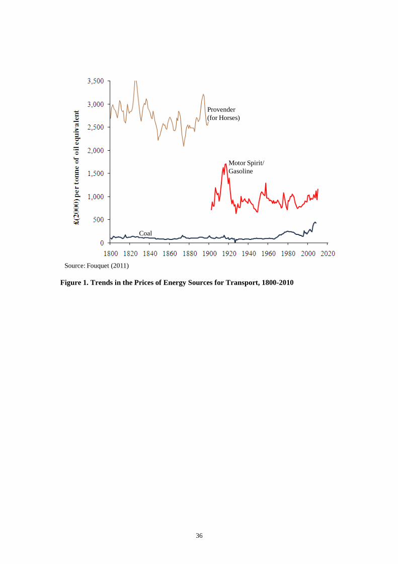
36
Motor Spirit/
Gasoline
Source: Fouquet (2011)
Coal
Provender
(for Horses)
Figure 1. Trends in the Prices of Energy Sources for Transport, 1800-2010
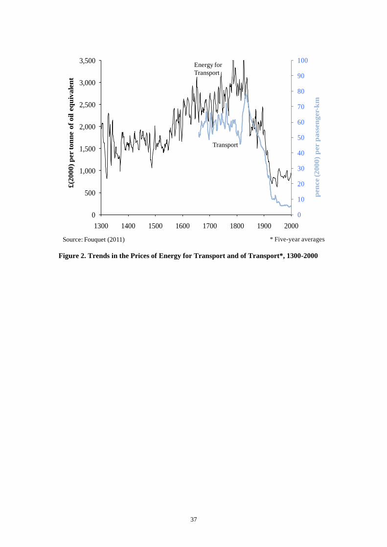
37
0
10
20
30
40
50
60
70
80
90
100
0
500
1,000
1,500
2,000
2,500
3,000
3,500
1300 1400 1500 1600 1700 1800 1900 2000
pen
ce (
200
0)
per p
ass
en
ger-
km
£(2
000)
per ton
ne o
f oil e
qu
ivale
nt
Energy for
Transport
Transport
* Five-year averagesSource: Fouquet (2011)
Figure 2. Trends in the Prices of Energy for Transport and of Transport*, 1300-2000
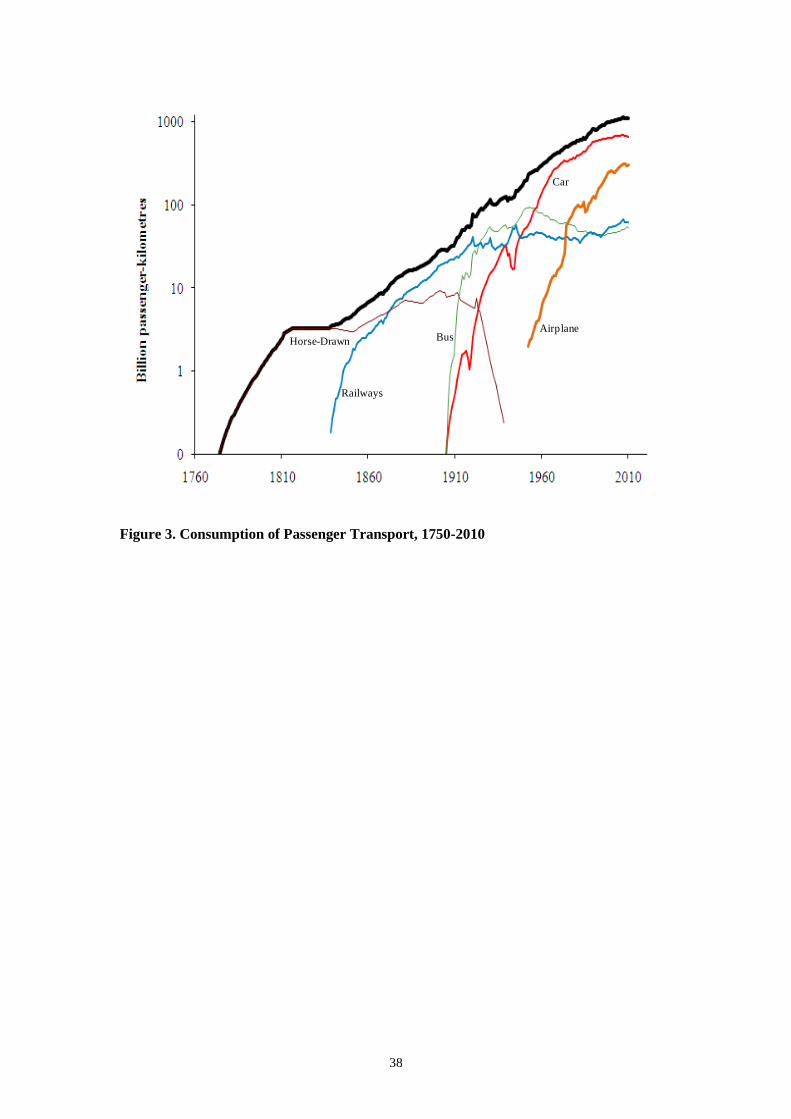
38
Horse-Drawn
Railways
Bus
Car
Airplane
Figure 3. Consumption of Passenger Transport, 1750-2010
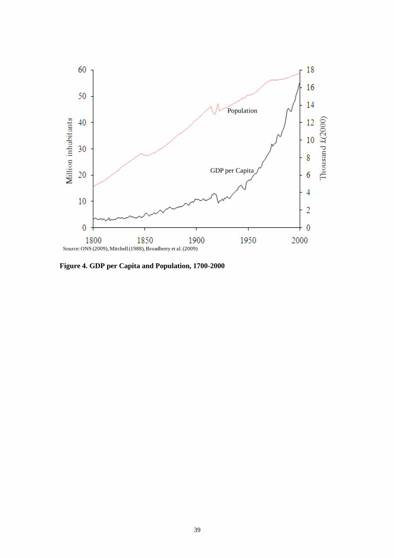
39
GDP per Capita
Population
Source: ONS (2009), Mitchell (1988), Broadberry et al. (2009)
Figure 4. GDP per Capita and Population, 1700-2000
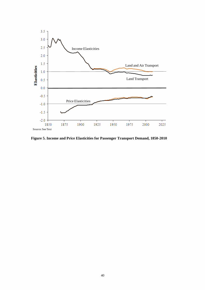
40
Price Elasticities
Income Elasticities
Source: See Text
Land and Air Transport
Land Transport
Figure 5. Income and Price Elasticities for Passenger Transport Demand, 1850-2010