Trends in the CERES Dataset, 2000–13: The Effects of Sea

Trends in the CERES Dataset, 2000–13: The Effects of Sea Ice and Jet Shifts andComparison to Climate Models

DENNIS L. HARTMANN AND PAULO CEPPI

Department of Atmospheric Sciences, University of Washington, Seattle, Washington

(Manuscript received 12 July 2013, in final form 7 November 2013)

ABSTRACT

The Clouds and the Earth’s Radiant Energy System (CERES) observations of global top-of-atmosphere

radiative energy fluxes for the period March 2000–February 2013 are examined for robust trends and vari-

ability. The trend in Arctic ice is clearly evident in the time series of reflected shortwave radiation, which

closely follows the record of ice extent. The data indicate that, for every 106 km2 decrease in September sea ice

extent, annual-mean absorbed solar radiation averaged over 758–908N increases by 2.5Wm22, or about

6Wm22 between 2000 and 2012. CMIP5 models generally show a much smaller change in sea ice extent over

the 1970–2012 period, but the relationship of sea ice extent to reflected shortwave is in good agreement with

recent observations. Another robust trend during this period is an increase in reflected shortwave radiation

in the zonal belt from 458 to 658S. This trend is mostly related to increases in sea ice concentrations in

the Southern Ocean and less directly related to cloudiness trends associated with the annular variability of

the Southern Hemisphere. Models from phase 5 of the Coupled Model Intercomparison Project (CMIP5)

produce a scaling of cloud reflection to zonal wind increase that is similar to trend observations in regions

separated from the direct effects of sea ice. Atmospheric Model Intercomparison Project (AMIP) model

responses over the Southern Ocean are not consistent with each other or with the observed shortwave

trends in regions removed from the direct effect of sea ice.

1. Introduction

The Clouds and the Earth’s Radiant Energy System

(CERES) experiment makes precise measurements of

Earth’s broadband solar and longwave irradiance (Loeb

et al. 2012a; Wielicki et al. 1996). The dataset is un-

precedented in its consistency and accuracy (Loeb et al.

2012b). Although a 13-yr record is short for climate

analysis, the dataset deserves a careful look to see what it

can tell us about connections within the climate system,

even though the changes we observe on such short time

scales are likely heavily influenced by natural variability.

Two things of interest that the dataset should be able

to measure are the sensitivity of the energy balance to

changing polar ice and the relationship of cloud albedo

to the position of the extratropical jet in the Southern

Hemisphere. We will begin by looking for statistically

significant linear trends in zonal–annual means of the

data and will then attempt tomake quantitative estimates

of the sensitivity of reflected solar radiation to sea ice

extent and the southern annular mode and compare with

climate model simulations.

2. Data and methods

The CERES data used are the monthly-mean Energy

Balanced and Filled (EBAF) version 2.7 data for the

period of March 2000 through February 2013, a period

of 13 yr. The time series of sea ice extent in September

was obtained from the National Snow and Ice Data

Center (Fetterer et al. 2009). We also make use of the

merged Hadley Centre–National Oceanic and Atmo-

spheric Administration (NOAA) optimum interpolated

(OI) sea surface temperature (SST) and sea ice concen-

tration dataset (Hurrell et al. 2008; Rayner et al. 2003).

These data are also boundary conditions for the Atmo-

spheric Model Intercomparison Project (AMIP) simula-

tions wewill use. The sea ice concentrationmeasurements

are based primarily on microwave satellite measurements

and should not be sensitive to the presence of clouds

of water or ice. The annular variability is characterized

by the upper tropospheric zonal wind averaged over

Corresponding author address:Dennis L. Hartmann, Department

of Atmospheric Sciences, University of Washington, Box 351640,

Seattle, WA 98195-1640.

E-mail: [email protected]

2444 JOURNAL OF CL IMATE VOLUME 27

DOI: 10.1175/JCLI-D-13-00411.1

� 2014 American Meteorological Society

mailto:[email protected]

458–658S, which is well correlated with other indices of an-

nular variability. Three-dimensional monthly-mean meteo-

rological fields were obtained from both the National

Centers for Environmental Prediction–National Center

for Atmospheric Research (NCEP–NCAR) reanalysis

dataset (Kalnay et al. 1996) and the European Centre for

Medium-Range Weather Forecasts (ECMWF) Interim

Re-Analysis (ERA-Interim) dataset (Dee et al. 2011).

To compare the observed changes with climate mod-

els, we analyze the output of 34 models from phase 5 of

the Coupled Model Intercomparison Project (CMIP5)

(Taylor et al. 2012), listed in the appendix. We combine

the historical and representative concentration pathway

(RCP) 8.5 integrations to yield time series for the period

March 1970–February 2013. We use this longer period

from the models so that the trend magnitude is more

robust and more comparable in size to the trend in the

data. The variables used are sea ice area fraction, out-

going top-of-atmosphere shortwave radiation, and zonal

wind, and the data are averaged annually. For eachmodel,

we use only the first ensemble member (‘‘r1i1p1’’). In

addition, we use AMIP runs from the CMIP5 archive.

To assess linear trends we use the methodology de-

scribed in Santer et al. (2008), which uses the theory

described in Sveshnikov (1968) and the formulas from

Bretherton et al. (1999) to estimate the degrees of free-

dom of an autoregressive-1 (AR-1) process. Uncertainties

are plotted for 5% and 95% confidence levels so that, if an

uncertainty bound is above (below) zero, the chance that

the trend is not positive (negative) is less than 5%. Lines

appearing in scatterplots were determined by principal

component analysis rather than ordinary least squares.

3. Results

a. Global trends

Figure 1 shows the linear trend of the annually and

zonally averaged reflected shortwave (SW) as a function

of latitude, along with the 5% and 95% confidence in-

tervals on the trend. The year is defined as the average of

March through February so that 13 12-month means can

be computed. Although trends are computed from a

12-yr difference, they are reported as change per decade.

The most robustly significant changes are a decreasing

trend over the Arctic and an increasing trend over the

Southern Ocean from 458 to 658S. The seasonal and lat-

itudinal distributions of these changes are illustrated in

Fig. 2, which shows a contour plot of the linear trend in

monthly-mean SW over 2000–12 as a function of latitude

and month. As expected, the shortwave trends in the

Arctic occur primarily in the spring and summer seasons.

The Arctic trend dips down to 608N in May, indicating

a significant contribution from earlier snowmelt in land

areas of the Arctic (Derksen and Brown 2012).

The spatial distribution of the trends in annual-mean

SW is shown in Fig. 3. Three features are of interest.

The negative trends in Arctic SW are greatest in the

Canadian and Siberian sectors but span the Arctic

Ocean. These changes are contributed mostly by the

summer half year inmiddle and high latitudes. Over the

FIG. 1. Trend in reflected shortwave computed from annual-

mean data and plotted as a function of latitude. The solid line

shows the linear trend difference over the period 2000–12 for the

zonal- and annual-mean reflected shortwave. The dashed lines

show the 5% and 95% confidence levels.

FIG. 2. Trend in reflected shortwave for 2000–12 computed from

monthly data and plotted as a function of latitude and month.

Contour interval is 2Wm22 decade21 and the zero contour is

omitted. Red contours indicate a reduction in reflected SW and

blue contours indicate an increase.

15 MARCH 2014 HARTMANN AND CEP P I 2445

Southern Ocean the reflected shortwave increases mod-

estly over a broad region between 458 and 658S in the

Indian and Pacific Ocean sectors. The trends at many

of these points are statistically significant, and no points

have statistically significant negative trends. The South-

ern Ocean trend is visible in every season as well, so it is

quite robust during this period. Some trends toward less

reflection can be seen along the coast of Antarctica and

in the Ross Sea that are related to declines in sea ice

there in the summer season. The effects of sea ice con-

centration trends in the Southern Ocean will be dis-

cussed more fully later.

The spatial structure of the trend in annual-mean

reflected shortwave in Fig. 3 strongly suggests a trend

toward La Ni~na conditions over this period, as indicated

by the decreasing reflection near the dateline and the

increased reflection west of the dateline and from an

analysis of sea surface temperature (not shown). The La

Ni~na trend also accounts for the upward trend in zonal-

mean SW between the equator and 108N in Fig. 1, since

as equatorial east Pacific SST cools during La Ni~na the

ITCZ is more concentrated north of the equator there.

A northward movement of the ITCZ would be con-

sistent with the greater absorption of energy in the

Northern Hemisphere accompanying the polar ice melt

following the reasoning of Chiang and Bitz (2005) and

Frierson and Hwang (2012), but the integrated effect of

this increasedArctic energy intake seems too small to be

important compared to the influence of ENSO during

the period of the CERES data.

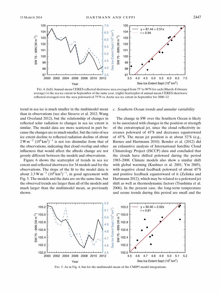
b. Arctic trends and sea ice

The trend over the Arctic is clearly related to the de-

cline in sea ice extent and associated snow cover during

this period. The climate feedbacks associated with ob-

served changes in surface ice have been recently assessed

by Flanner et al. (2011). The left panel of Fig. 4 shows

the September sea ice extent and the annual-mean SW

averaged over the area poleward of 758N as a function of

year. The right panel shows a scatterplot of the same

two quantities. From the linear fit in Fig. 4, we infer that,

for each million square kilometers (106 km2) of sea ice

extent removed, the SW at the top of the atmosphere

averaged poleward of 758Ndecreases by about 2.5Wm22.

That translates into an albedo change of about 0.013

(106 km2)21. These are annual averages, and the changes

are much larger in summer. The polar cap albedo de-

clined by about 0.034 or about 6% between 2000 and

2012, while the sea ice extent in September declined

about 40%. The change in mean solar absorption pole-

ward of 758N over this period is about 6Wm22 for the

annual mean and 20Wm22 for the June throughAugust

average. FromFig. 4 it is clear that year-to-year variations

in SW over the pole are closely related to sea ice extent.

Changes in clouds may also have an influence, primarily

by screening the surface albedo changes from affecting

the top-of-atmosphere budget as much as they might,

but there may also be changes in cloudiness associated

with the sea ice change.We have not attempted to assess

cloud changes, except to note that the observed top-of-

atmosphere response to sea ice extent is reasonably well

simulated by models (Kay and Gettelman 2009). CERES

clear-sky estimates suggest that about half of the surface

albedo decrease because ice melt is screened by clouds

and thereby not apparent at the top of the atmosphere

(N. Loeb 2013, personal communication).

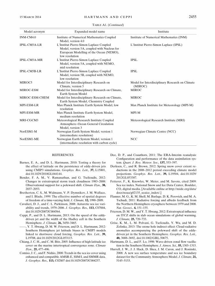
Figure 5 shows the same data as Fig. 4, except for the

multimodel mean of the CMIP5 models. The downward

FIG. 3. Linear trend of CERES annual-mean reflected shortwave computed for each 18 3 18region of the globe (Wm22 decade21).


trend in sea ice is much smaller in the multimodel mean

than in observations (see also Stroeve et al. 2012; Wang

and Overland 2012), but the relationship of changes in

reflected solar radiation to changes in sea ice extent is

similar. The model data are more scattered in part be-

cause the changes are somuch smaller, but the ratio of sea

ice extent decline to reflected radiation decline of about

2Wm22 (106 km2)21 is not too dissimilar from that of

the observations, indicating that cloud overlap and other

influences that would affect the albedo change are not

grossly different between the models and observations.

Figure 6 shows the scatterplot of trends in sea ice

extent and reflected shortwave for 34 models and for the

observations. The slope of the fit to the model data is

about 2.3Wm22 (106 km2)21, in good agreement with

Fig. 5. The models and the data are on the same line, but

the observed trends are larger than all of the models and

much larger than the multimodel mean, as previously

shown.

c. Southern Ocean trends and annular variability

The change in SW over the Southern Ocean is likely

to be associated with changes in the position or strength

of the extratropical jet, since the cloud reflectivity in-

creases poleward of 458S and decreases equatorward

of 458S. The mean jet position is at about 528S (e.g.,

Barnes and Hartmann 2010). Bender et al. (2012) did

an exhaustive analysis of International Satellite Cloud

Climatology Project (ISCCP) data and concluded that

the clouds have shifted poleward during the period

1983–2008. Climate models also show a similar shift

with global warming (Kushner et al. 2001; Yin 2005),

with negative cloud feedback poleward of about 458Sand positive feedback equatorward of it (Zelinka and

Hartmann 2012), which may be related to a poleward jet

shift as well as thermodynamic factors (Tsushima et al.

2006). In the present case, the long-term temperature

and ozone trends during this period are small and the

FIG. 4. (left) Annual-mean CERES reflected shortwave area averaged from 758 to 908N for each (March–February

average) vs the sea ice extent in September of the same year. (right) Scatterplot of annual-mean CERES shortwave

reflected averaged over the area poleward of 758N vs Arctic sea ice extent in September for 2000–12.

FIG. 5. As in Fig. 4, but for the multimodel mean of the CMIP5 model integrations.


trend we see is most likely to be associated with natural

variability, possibly because of the trend toward LaNi~na

conditions.

To show the relationship of the SW trend to circulation

changes, we compute the trends of meteorological fields

over the Southern Hemisphere and see that they reflect

a change in meteorology that can be logically associated

with the shortwave trends. Figure 7 shows the trend in

zonal wind averaged over the 700–300-hPa layer in the

same format as Fig. 1. Statistically significant trends occur

over the Southern Ocean, with increasing winds in the

band from 458 to 658S and decreasing winds to the north

and south of that. Trends are shown for both NCEP–

NCAR and ERA-Interim reanalyses to demonstrate that

these trends are not very sensitive to the dataset used,

although the ERA-Interim trend is smaller. The wind

increases by about 2ms21, while the SW increases by

about 2Wm22, giving a simple one-to-one scaling of the

annual-mean wind increase with the SW increase of

1Wm22 (ms21)21 of wind increase. The relationship of

cloud shortwave reflection to a poleward wind shift, with

increased solar reflection poleward of the jet and de-

creased solar reflection equatorward of it, may help to

enhance or sustain the poleward movement of the jet,

since cloud radiative effects influence the latitude of the

jet in CMIP5 simulations (Ceppi et al. 2012).

While the SW trend signal is strongest in Southern

Hemisphere (SH) summer because of the seasonal varia-

tion of insolation, thewind trend signature shows no strong

seasonal preference, with thewesterly intensification trend

over the Southern Ocean apparent in every season (not

shown). In this time period the zonal wind over the

Southern Ocean in summer is somewhat correlated with

the zonal wind during the previous winter. A statistically

significant reduction in zonal winds is also seen near

708N, which comes primarily from the Northern Hemi-

sphere (NH) spring and summer season and may be

related to the ice melt in the Arctic (Ogi and Wallace

2012; Screen et al. 2013). A westerly trend is also ap-

parent around 158N and is likely related to the La Ni~na

trend, which concentrates more convective heating and

Rossby wave driving north of the equator.

As an index of southern annular mode variability we

have considered the Antarctic Oscillation index (AAO)

as well as zonal averages of zonal wind averaged over

700–300 hPa between 458 and 658S. These two indices

are correlated with each other at 0.95. For the tropo-

spheric wind index we hereafter use the ERA-Interim

zonal winds averaged over 300–700 hPa and area aver-

aged over 458–658S.Despite the strongly suggestive temporal trends of

SW and zonal wind in the band from 458 to 658S it ap-

pears that the robust linear trend in SW is more strongly

connected to Antarctic sea ice than to the zonal winds.

Satellite data indicate that sea ice concentration around

Antarctica has been increasing (Cavalieri and Parkinson

2008; Comiso and Nishio 2008; Parkinson and Cavalieri

2012; Screen 2011). The increase in sea ice concen-

tration in the band from 558 to 658S appears to be

a substantial contributor to the increase in shortwave

reflection over the period from 2000 to 2012 for which

FIG. 6. Trend from 2000 to 2012 for 758–908N reflected shortwave

vs same trend for sea ice extent. Solid circles indicate the trends

calculated from 34 CMIP5 models. The open circle represents

observations not included in the regression shown.FIG. 7. As in Fig. 1, but for the trend of annual-mean zonal wind

fromNCEP–NCAR reanalysis averaged over the 700–300-hPa layer.

The dashed line shows a comparable trend for ERA-Interim.


we have CERES observations. Figure 8 shows the

annual-mean reflected shortwave and sea ice concen-

tration, which both have increasing trends over this

period. Sea ice concentrations also increase poleward

of 658S, but we limit consideration to 558–658S since

this includes all the sea ice variations within the band

where the SW increases with time. The trend in sea ice

is a major contributor to the trend in SW in the band

from 458 to 658S during the period, but the trend in SW

extends beyond the region that is directly influenced

by sea ice (Figs. 1–3).

Table 1 shows the correlation matrix between various

indices that are likely involved in the trends observed.

For a sample size of 13 annual means, the 5% and 95%

confidence limits on correlation are 60.48, using a null

hypothesis that the true correlation is zero. We have

chosen the band from 458 to 658S for SW and winds,

since these are where the records show significant

trends and also because these latitudes correspond to

the poleward lobe of wind variations associated with the

southern annular mode (e.g., Hartmann and Lo 1998).

Table 1 indicates strong correlations of SW with sea ice

concentration and also significant correlations with tro-

pospheric wind. The correlation with wind is still sig-

nificant if the temporal trend is first removed from the

data. Also shown is that stratospheric winds are signifi-

cantly correlated with tropospheric winds, and Ni~no-

3.4 is significantly correlated with both tropospheric

and stratospheric winds. The connection between tro-

pospheric and stratospheric annular variability is well

established for both hemispheres (Thompson and

Wallace 2000). L’Heureux and Thompson (2006) found

that about 25% of the Southern Hemisphere annular

variability was related to ENSO. The connection of the

annular variability to ENSO in the Southern Hemi-

sphere has recently been discussed by Lin et al. (2012),

who showed that the stationary wave variability in the

extratropics increases during La Ni~na conditions, mostly

through the meridional propagation in the troposphere.

The stationary wave variability then establishes a link to

the stratosphere. The mechanisms are increasingly better

understood whereby the Hadley cell expands during La

Ni~na (Seager et al. 2003) and the extratropical eddy-

driven jet shifts north and southwith theHadley cell edge

(Kang and Polvani 2011; Ceppi andHartmann 2013). It is

therefore expected that themidlatitudewesterly jet in the

troposphere and stratosphere would be shifted poleward

and intensified by La Ni~na conditions.

Figure 9 shows the trend of the 700–300-hPa zonalwind

in the CMIP5 models during 1970–2012, along with the

trend in observed wind repeated from Fig. 7. The ob-

served wind trend is much stronger, primarily because

the natural variability in 2000–12 trended strongly toward

a positive annular mode during this period. Figure 9 also

shows the trend in shortwave in the models along with

a rescaling of the shortwave trend to estimate what the

FIG. 8. Observed annual mean of SW averaged from 458 to 658S and sea ice concentration averaged from 558 to 658S(left) plotted vs year from 2000 to 2012 and (right) as a scatterplot.

TABLE 1. Correlation matrix for annual-mean values of some

selected indices. Tropospheric wind (U Trop) is averaged over

300–700hPa and stratospheric wind (U Strat) is for 10 hPa. All

latitude bands are area-weighted averages. Correlations larger

than 0.48 are considered significant (see text).

SW

458–658SSea ice

558–658SU Trop

458–658SU Strat

458–658S Ni~no-3.4

SW 458–658S 1

Sea ice

558–658S0.76 1

U Trop

458–658S0.51 0.40 1

U Strat

458–658S0.29 0.35 0.63 1

Ni~no-3.4 20.13 20.40 20.53 20.55 1


model shortwave trendwould be if themultimodel-mean

wind shift was as large as the NCEP–NCAR change in

the left panel. The rescaled model shortwave trends

agree with the observations between 308 and 508S but

depart significantly from observations outside this in-

terval. The models produce a significant hemispherically

integrated net reduction in reflected shortwave in asso-

ciation with a poleward shift of the jet, whereas we will

see in section 3d that the observed changes in reflected

solar radiation tend to integrate to a smaller number,

although the observed trend in SWat higher latitudes has

contributions from sea ice change that are not included

in the model results. Of course the CMIP5 simulated

changes over 1970–2012 are likely driven by different

mechanisms than drive the mostly natural interannual

variability in the observed trends over 2000–12. For

global warming it might be expected that the declining

sea ice trends in the Antarctic would be opposite to the

increasing Antarctic sea ice observed in 2000–12, and this

explains much of the discrepancy between CMIP5models

and the observations between 558 and 708S in Fig. 9.

As a further comparison with models we show in

Fig. 10 the trend in SW over 2000–08 from the AMIP

simulations from the CMIP5 archive, along with the

trend in sea ice concentration from the merged Hadley

Centre–NOAA OI dataset and the SW trend from

CERES over the same period. The CMIP5 AMIP ar-

chive stops in 2008, so we compare for the shorter period

in which CERES andAMIP overlap. The regions of best

agreement for SW between AMIP and observations are

in the polar regions, where the observed sea ice con-

centrations were used to force the AMIP models. Some

of the tropical signature associated with ENSO is also

captured, but the trends in SW over the Southern Ocean

midlatitudes that appear to be associated with annular

mode variations are not captured by the AMIP simula-

tions. It is tempting to conclude that the models are not

capturing the SW response to ENSO in the extratropics,

but the record is short and the level of natural variability

of the southern annular mode is large.

Figure 11 shows the trend of zonal-mean OLR over

the 2000–12 period as a function of latitude. In high

southern latitudes it has a similar shape to the year-to-

year variability and its structure is consistent with a

poleward jet shift and intensification. The most signif-

icant features are an increase of OLR over the Arctic,

FIG. 9. Comparison of the observed annual-mean trends during 2000–12 (red line) and from CMIP5 models over

the 1970–2012 period (gray lines) for (left) zonal-mean wind averaged for 700–300hPa and (right) the SW trend. The

black line represents the multimodel mean, and the dashed line represents the model means rescaled to the observed

zonal wind change at 608S.

FIG. 10. Trends over the 2000–08 period for SW in AMIPmodels

(dashed), SW from CERES (solid), and sea ice concentration from

the merged Hadley Centre–NOAA OI dataset (blue). All are

based on annual-mean data.


which we can associate with ice melting, and a decrease

just north of the equator in association with the El Ni~no

trend over this period. The outgoing longwave radia-

tion (OLR) shows a much more robust connection to

the annular mode variability than the SW. The corre-

lation between OLR over 608–908S and tropospheric

zonal wind over 458–658S is 0.91. This high correlation

is because the jet shift has a strong signature in the

temperature field, via the thermal wind relationship. As

the jet shifts poleward and simultaneously intensifies,

the air becomes cooler poleward of the jet and the OLR

decreases with this cooling. Cloud changes may also

contribute to the change in OLR, but this contribution is

likely of the same sign and smaller than the effect of

temperature. The air cools by sinking less, which might

be expected to give an increase in high clouds, further

contributing to the reduction in OLR but probably

marginally so compared to the direct temperature ef-

fect. The cloud reflectivity depends less sensitively on

the zonal jet structure, since the dominant cloud type

for reflection is low cloud. Low clouds are in large part

driven by the vertical exchange of energy in the boundary

layer, so they are less directly linked to zonal wind shifts

than temperature and OLR. Figure 12 shows a close re-

lationship between the annual-mean tropospheric wind

at 458–658S and the OLR averaged over the area of the

polar cap from 608 to 908S. This signature is slightly

stronger in the winter season (not shown).

d. Area averages and northward transports

To quantify how the trends in shortwave reflection af-

fect larger areas, we integrate the trends in Fig. 1 over the

north and south polar caps as in (1), where u is latitude

and x5 sinu. The term S[ represents the trend in SW,

FSP(u)5

ðsinu21

S[ dx

ðsinu21

dx

and FNP(u)5

ð1sinu

S[ dx

ð1sinu

dx

. (1)

These integrals as functions of latitude are shown in

Fig. 13. Following the south polar cap integral (blue line),

one can see that the contributions to increased reflection

in the 458–658S band are very nearly canceled by the

trends of opposite sign in the 208–458S band, so that not

much net change results from the SouthernOcean trends,

FIG. 11. As in Fig. 1, but for OLR.

FIG. 12. (left) OLR averaged for the region 608–908S and the tropospheric wind index for 458–658S annual-average

anomalies vs year and (right) scatterplot of the same quantities with the linear fit (R 5 0.91).


which are associated partly with sea ice concentration

increases and partly with the cloud response to a jet

shift. The trend in global-mean reflected solar radiation

is most easily read from the south polar cap integral at

the North Pole and is about 20.1Wm22. The area av-

erage of the integral of SW trend over the south polar cap

reaches a maximum of 10.86Wm22 decade21 at 508S,which implies an increase in the required poleward en-

ergy flux of about 0.06 PW or about 1% of the total

poleward flux. The area-average SW trend poleward

of 348S is zero and reaches a maximum negative value

(increased solar absorption) of 20.16Wm22 decade21

at 278S, indicating a rather small net energy gain in the

Southern Hemisphere. A significant difference between

the observed south polar cap integral and the equivalent

calculation for the rescaled model response in Fig. 9 is

the weakness of the increased reflection between 458 and658S in the models. In consequence of this, the model

integral is about 20.6Wm22 at 308S, where the obser-

vational integral is only 20.1Wm22 decade21. A signif-

icant portion of this difference is related to the increase in

sea ice concentration in high southern latitudes, which

does not occur in the simulations.

Polvani and Smith (2013) suggest that the Antarctic

sea ice trends are within the range expected from natu-

ral variability exhibited by CMIP5 simulations. Sea ice

variations are known to occur in conjunction with the

annular mode. In both the long-term trend (Parkinson

and Cavalieri 2012) and in the response to the southern

annular mode and ENSO (Lefebvre et al. 2004; Liu et al.

2004; Simpkins et al. 2012), changes of opposite sign tend

to occur in the Ross Sea area and the Bellingshausen/

Amundsen Seas area. Modeling suggests that the asym-

metries in the sea ice response can be explained by

asymmetries in the mechanical and thermal forcing

of sea ice by annular mode variability (Lefebvre and

Goosse 2005; Sen Gupta and England 2006; Turner et al.

2009). The sea ice trends over the 2000–12 period are

more zonally symmetric (not shown). Lefebvre andGoosse

(2008) argue that during winter each Antarctic sea ice

sector changes independently.

For the north polar cap integral (red line in left panel

of Fig. 4) the polar cap area average is initially quite

large (26Wm22) and gradually decreases to near zero

at the equator. Note that the scales for the two hemi-

spheres are quite different. As one proceeds south

across the equator, trends in southern midlatitudes

cause a small reduction in global reflection from 208 to458S, which is then erased by the trends in the 458–658Sband, indicating the energetic significance of the high-

latitude sea ice and cloud brightening.

The right panel in Fig. 13 shows the changes in the im-

plied northward energy flux from the trends in shortwave,

longwave, and net radiation, assuming that the northward

flux balances the trends at the top of the atmosphere. The

global mean of 20.1Wm22 decade21 was removed prior

to this calculation. The reduction in northward flux implied

by the shortwave trends is offset by trends in longwave

emission, so that the reduction in flux implied by the net

radiation is considerably less. Although the gradient in flux

is largest over theArctic regionwhere the decreases in SW

are greatest, the flux anomalies continue to increase all the

way to 308N. The extension to lower latitudes is contrib-

uted by the small reductions of SW in the midlatitudes,

whose genesis is unclear to us. In the Southern Hemi-

sphere the compensation between SW and longwave

trends is less, so that the increase in poleward flux is of the

same magnitude as in the Northern Hemisphere, though

FIG. 13. (left) Integrals of reflected solar radiation trends over the southern and northern polar caps as

functions of latitude and (right) trends of northward energy flux implied by the trends in top-of-atmosphere

energy flux.


the changes in shortwave flux are smaller in the Southern

Hemisphere.

4. Summary and discussion

The 13-yr record of CERES earth radiation budget

measurements, although relatively short for climate

purposes, reveals three statistically significant linear

trends of annual means over the 2000–12 period.

These are related to 1) the declining Arctic sea ice,

2) increasing sea ice concentrations and shifting of the

zonal wind pattern over the Southern Ocean, and

3) ENSO variability. Based on the linear trend of annual

means, we estimate that a reduction in September

Arctic sea ice extent of 106 km2 results in an increase in

solar absorption over the polar cap from 758 to 908N of

2.5Wm22 or an albedo decrease of about 0.013. Al-

though sea ice trends in the CMIP5 model ensemble

are much smaller than observed during the interval

2000–12, the relationship between sea ice decline and

reflected solar radiation is similar, indicating that ice

albedo changes and their relationship with cloud albedo

are reasonably treated in the models.

CERES and reanalysis data from 2000 to 2012 indicate

that, for annual means, increasing upper-level zonal winds

in the latitude band from 458 to 658S by 1ms21 result in

an increase in shortwave reflection of about 1Wm22 in

the same band, but a significant portion of the increased

reflection is associated with increasing Antarctic sea ice

during this period. Decreases in reflected radiation occur

in other latitudes, however, such that the hemispheric-

average shortwave reflection is virtually unchanged.

While models capture some of the trends associated with

annular mode variability in the Southern Hemisphere,

the increased reflectivity in high latitudes associated with

sea ice is not a feature of CMIP5 global warming simu-

lations. They simulate reduced reflection equatorward of

458S of about the observed magnitude but produce much

less brightening poleward of 558S than is observed during

the 2000–12 period.

Grise et al. (2013, hereafter G13) presented radiation

budget changes associated with the positive (poleward)

shift of the southern annular mode (SAM) index in sim-

ulations with the CAM3 model and compare with ISCCP

cloud changes. The pattern of response they obtain is quite

different than the trend in Fig. 1 and gives amuch stronger

impact on the hemispheric energy balance. They find a

decrease of cloud reflection across 358–608S and an in-

crease in reflection from 158 to 358S, whereas the trend in

Fig. 1 is an increase of reflection from 458 to 708S and

a decrease from 258 to 458S, so that these structures are

nearly orthogonal to each other. G13 considered the

December–February season, whereas Fig. 1 shows the

annual mean. We find that the structure of the trend for

the December–February mean is similar to the annual

mean in Fig. 1, with slightly larger trends and greater

uncertainty. If we regress the zonal-mean SW onto the

458–658S wind index we have used here, the regressions

for the annual mean and December–January mean are

quite noisy but do show a brightening of clouds in the

458–658S band similar to the trend. The noisy rela-

tionship between indices of the annular mode and the

CERES SW indicates that the annular mode is not

a dominant influence on the zonal-mean SWduring this

period. If we regress the zonal winds and SW in the

CMIP5 models against an index of the southern annu-

lar mode, the multimodel mean shows a reduction of

cloud reflection equatorward of the jet but no sub-

stantial increase poleward of the jet, in basic agreement

with the analysis of G13 (not shown).

In contrast, the trend of OLR found here is in good

agreement with the structure found by G13 and in the

regressions of the multimodel CMIP5 simulations, with

a reduction of OLR poleward of about 508S and an in-

crease around 308–458S, which appear to follow the

temperature changes required by thermal wind. This

suggests that the structure of the large-scale dynamical

shift is similar in the observations shown here, in G13

and in CMIP5, but that the shift in shortwave reflection

is very different. This would be consistent with the great

diversity of climate model responses in Fig. 9 and with

the general wisdom that cloud shortwave responses are

uncertain and vary greatly from model to model (e.g.,

Ceppi et al. 2012).

An assessment of the robustness of the trends seen in

the 2000–13 period is difficult without a longer dataset.

Since the period of record is short and the trends in wind

and SW in the Southern Hemisphere seem to be influ-

enced in part by ENSO changes and in part by as yet

unexplained increases in sea ice concentration, it would

be dangerous to assume that the relationships found

here would apply to climate change or other forms of

annular variability. In particular, it is not certain that

the data presented here give a robust estimate of what

cloud responses we should expect from a shift in the

southern annular mode, since sea ice and other things

are changing at the same time.

Acknowledgments. The authors thank Kevin Grise,

Norman Loeb, Angie Pendergrass, and an anonymous

reviewer for helpful suggestions. The CERES data were

obtained from the NASA Langley Research Center

Atmospheric Science Data Center. Reanalysis data were

obtained from NOAA and ECMWF web resources. The

authors were supported byNSFGrantAGS-0960497 and

NASA Grant NNX09AH73G.


APPENDIX

CMIP5 models used in the analysis

A list of the 34 CMIP5models analyzed, their expanded names, and the institutions responsible for themodels are

in Table A1.

TABLE A1. List of CMIP5 models used in the analysis.

Model acronym Expanded model name Institute

ACCESS1.0 Australian Community Climate and Earth-System

Simulator, version 1.0

Commonwealth Scientific and Industrial Research

Organisation (CSIRO)–Bureau of Meteorology

(BOM)

ACCESS1.3 Australian Community Climate and Earth-System

Simulator, version 1.3

CSIRO–BOM

BCC-CSM1.1 Beijing Climate Center, Climate System Model,

version 1.1

Beijing Climate Center (BCC)

BCC-CSM1.1(m) Beijing Climate Center, Climate System Model,

version 1.1(m)

BCC

BNU-ESM Beijing Normal University–Earth System Model College of Global Change and Earth System

Science (GCESS), Beijing Normal University

CanESM2 Second Generation Canadian Earth System

Model

Canadian Centre for Climate Modelling and

Analysis (CCCma)

CCSM4 Community Climate System Model, version 4 NCAR

CESM1 (BGC) Community Earth System Model, version 1

(Biogeochemistry)

National Science Foundation (NSF)–U.S.

Department of Energy (DOE)–NCAR

CESM1 (CAM5) Community Earth System Model, version 1

(Community Atmosphere Model, version 5)

NSF–DOE–NCAR

CMCC-CESM Centro Euro-Mediterraneo per I Cambiamenti

Climatici Carbon Earth System Model

Centro Euro-Mediterraneo per I Cambiamenti

Climatici (CMCC)

CMCC-CM Centro Euro-Mediterraneo per I Cambiamenti

Climatici Climate Model

CMCC

CNRM-CM5 Centre National de Recherches M�et�eorologiques

Coupled Global Climate Model, version 5

Centre National de Recherches M�et�eorologiques

(CNRM)–Centre Europ�een de Recherche et de

Formation Avanc�ee en Calcul Scientifique

(CERFACS)

CSIRO Mk3.6.0 Commonwealth Scientific and Industrial Research

Organisation Mark, version 3.6.0

CSIRO– Queensland Climate Change Centre of

Excellence (QCCCE)

FGOALS-g2 Flexible Global Ocean–Atmosphere–Land

System Model gridpoint, version 2

State Key Laboratory of Numerical Modeling for

Atmospheric Sciences and Geophysical Fluid

Dynamics (LASG)–Center for Earth System

Science (CESS)

GFDL CM3 Geophysical Fluid Dynamics Laboratory Climate

Model, version 3

NOAA/Geophysical Fluid Dynamics Laboratory

(GFDL)

GFDL-ESM2G Geophysical Fluid Dynamics Laboratory Earth

System Model with Generalized Ocean Layer

Dynamics component

NOAA/GFDL

GFDL-ESM2M Geophysical Fluid Dynamics Laboratory Earth

System Model with Modular Ocean Model 4

component

NOAA/GFDL

GISS-E2H Goddard Institute for Space Studies Model E2,

coupled with the Hybrid Coordinate Ocean

Model (HYCOM)

National Aeronautics and Space Administration

(NASA) Goddard Institute for Space Studies

(GISS)

GISS-E2-R Goddard Institute for Space Studies Model E2,

coupled with the Russell ocean model

NASA GISS

HadGEM2-AO Hadley Centre Global Environment Model,

version 2–Atmosphere and Ocean

National Institute of Meteorological Research

(NIMR), Korea Meteorological Administration

(KMA)

HadGEM2-CC Hadley Centre Global Environment Model,

version 2–Carbon Cycle

Met Office (UKMO) Hadley Centre

HadGEM2-ES Hadley Centre Global Environment Model,

version 2–Earth System

UKMO Hadley Centre


REFERENCES

Barnes, E. A., and D. L. Hartmann, 2010: Testing a theory for

the effect of latitude on the persistence of eddy-driven jets

using CMIP3 simulations. Geophys. Res. Lett., 37, L15801,

doi:10.1029/2010GL044144.

Bender, F. A. M., V. Ramanathan, and G. Tselioudis, 2012:

Changes in extratropical storm track cloudiness 1983–2008:

Observational support for a poleward shift. Climate Dyn., 38,

2037–2053.

Bretherton, C. S., M. Widmann, V. P. Dymnikov, J. M. Wallace,

and I. Blade, 1999: The effective number of spatial degrees

of freedom of a time-varying field. J. Climate, 12, 1990–2009.

Cavalieri, D. J., and C. L. Parkinson, 2008: Antarctic sea ice vari-

ability and trends, 1979–2006. J. Geophys. Res., 113, C07004,doi:10.1029/2007JC004564.

Ceppi, P., and D. L. Hartmann, 2013: On the speed of the eddy-

driven jet and the width of the Hadley cell in the Southern

Hemisphere. J. Climate, 26, 3450–3465.——, Y. T. Hwang, D. M. W. Frierson, and D. L. Hartmann, 2012:

Southern Hemisphere jet latitude biases in CMIP5 models

linked to shortwave cloud forcing. Geophys. Res. Lett., 39,

L19708, doi:10.1029/2012GL053115.

Chiang, J. C. H., and C. M. Bitz, 2005: Influence of high latitude ice

cover on the marine intertropical convergence zone. Climate

Dyn., 25, 477–496.Comiso, J. C., and F. Nishio, 2008: Trends in the sea ice cover using

enhanced and compatible AMSR-E, SSM/I, and SMMR data.

J. Geophys. Res., 113, C02S07 doi:10.1029/2007JC004257.

Dee, D. P., and Coauthors, 2011: The ERA-Interim reanalysis:

Configuration and performance of the data assimilation sys-

tem. Quart. J. Roy. Meteor. Soc., 137, 553–597.

Derksen, C., and R. Brown, 2012: Spring snow cover extent re-

ductions in the 2008–2012 period exceeding climate model

projections. Geophys. Res. Lett., 39, L19504, doi:10.1029/

2012GL053387.

Fetterer, F., K. Knowles, W. Meier, and M. Savoie, cited 2009:

Sea ice index. National Snow and Ice Data Center, Boulder,

CO, digital media. [Available online at http://nsidc.org/data/

docs/noaa/g02135_seaice_index/.]

Flanner, M. G., K. M. Shell, M. Barlage, D. K. Perovich, andM. A.

Tschudi, 2011: Radiative forcing and albedo feedback from

the Northern Hemisphere cryosphere between 1979 and 2008.

Nat. Geosci., 4, 151–155.Frierson, D.M.W., and Y. T. Hwang, 2012: Extratropical influence

on ITCZ shifts in slab ocean simulations of global warming.

J. Climate, 25, 720–733.

Grise, K. M., L. M. Polvani, G. Tselioudis, Y. Wu, and M. D.

Zelinka, 2013: The ozone hole indirect effect: Cloud-radiative

anomalies accompanying the poleward shift of the eddy-

driven jet in the Southern Hemisphere. Geophys. Res. Lett.,

40, 3688–3692, doi:10.1002/GRL.50675.

Hartmann, D. L., and F. Lo, 1998: Wave-driven zonal flow vacilla-

tion in the Southern Hemisphere. J. Atmos. Sci., 55, 1303–1315.

Hurrell, J. W., J. J. Hack, D. Shea, J. M. Caron, and J. Rosinski,

2008: A new sea surface temperature and sea ice boundary

dataset for the CommunityAtmosphereModel. J. Climate, 21,

5145–5153.

TABLE A1. (Continued)

Model acronym Expanded model name Institute

INM-CM4.0 Institute of Numerical Mathematics Coupled

Model, version 4.0

Institute of Numerical Mathematics (INM)

IPSL-CM5A-LR L’Institut Pierre-Simon Laplace Coupled

Model, version 5A, coupled with Nucleus for

European Modelling of the Ocean (NEMO),

low resolution

L’Institut Pierre-Simon Laplace (IPSL)

IPSL-CM5A-MR L’Institut Pierre-Simon Laplace Coupled

Model, version 5A, coupled with NEMO,

mid resolution

IPSL

IPSL-CM5B-LR L’Institut Pierre-Simon Laplace Coupled

Model, version 5B, coupled with NEMO,

low resolution

IPSL

MIROC5 Model for Interdisciplinary Research on

Climate, version 5

Model for Interdisciplinary Research on Climate

(MIROC)

MIROC-ESM Model for Interdisciplinary Research on Climate,

Earth System Model

MIROC

MIROC-ESM-CHEM Model for Interdisciplinary Research on Climate,

Earth System Model, Chemistry Coupled

MIROC

MPI-ESM-LR Max Planck Institute Earth System Model, low

resolution

Max Planck Institute for Meteorology (MPI-M)

MPI-ESM-MR Max Planck Institute Earth System Model,

medium resolution

MPI-M

MRI-CGCM3 Meteorological Research Institute Coupled

Atmosphere–Ocean General Circulation

Model, version 3

Meteorological Research Institute (MRI)

NorESM1-M Norwegian Earth System Model, version 1

(intermediate resolution)

Norwegian Climate Centre (NCC)

NorESM1-ME Norwegian Earth System Model, version 1

(intermediate resolution with carbon cycle)

NCC


http://nsidc.org/data/docs/noaa/g02135_seaice_index/

http://nsidc.org/data/docs/noaa/g02135_seaice_index/

Kalnay, E., and Coauthors, 1996: The NCEP/NCAR 40-Year Re-

analysis Project. Bull. Amer. Meteor. Soc., 77, 437–471.

Kang, S. M., and L. M. Polvani, 2011: The interannual relationship

between the latitude of the eddy-driven jet and the edge of the

Hadley cell. J. Climate, 24, 563–568.

Kay, J. E., and A. Gettelman, 2009: Cloud influence on and re-

sponse to seasonal Arctic sea ice loss. J. Geophys. Res., 114,

D18204, doi:10.1029/2009JD011773.

Kushner, P. J., I. M. Held, and T. L. Delworth, 2001: Southern

Hemisphere atmospheric circulation response to global

warming. J. Climate, 14, 2238–2249.

Lefebvre, W., and H. Goosse, 2005: Influence of the southern an-

nular mode on the sea ice-ocean system: The role of the

thermal and mechanical forcing. Ocean Sci., 1, 145–157.

——, and ——, 2008: An analysis of the atmospheric processes

driving the large-scale winter sea ice variability in the

Southern Ocean. J. Geophys. Res., 113, C02004, doi:10.1029/

2006JC004032.

——,——,R. Timmermann, and T. Fichefet, 2004: Influence of the

southern annular mode on the sea ice–ocean system. J. Geo-

phys. Res., 109, C09005, doi:10.1029/2004JC002403.

L’Heureux, M. L., and D. W. J. Thompson, 2006: Observed rela-

tionships between the El Ni~no–Southern Oscillation and the

extratropical zonal-mean circulation. J. Climate, 19, 276–287.

Lin, P., Q. Fu, and D. L. Hartmann, 2012: Impact of tropical SST

on stratospheric planetary waves in the Southern Hemisphere.

J. Climate, 25, 5030–5046.

Liu, J. P., J. A. Curry, and D. G. Martinson, 2004: Interpretation of

recent Antarctic sea ice variability. Geophys. Res. Lett., 31,

L02205, doi:10.1029/2003GL018732.

Loeb, N. G., S. Kato, W. Su, T. Wong, F. G. Rose, D. R. Doelling,

J. R. Norris, and X. Huang, 2012a: Advances in understanding

top-of-atmosphere radiation variability from satellite obser-

vations. Surv. Geophys., 33, 359–385.——, J. M. Lyman, G. C. Johnson, R. P. Allan, D. R. Doelling,

T. Wong, B. J. Soden, and G. L. Stephens, 2012b: Observed

changes in top-of-the-atmosphere radiation and upper-

ocean heating consistent within uncertainty. Nat. Geosci.,

5, 110–113.

Ogi, M., and J. M. Wallace, 2012: The role of summer surface wind

anomalies in the summer Arctic sea ice extent in 2010 and

2011.Geophys. Res. Lett., 39,L09704, doi:10.1029/2012GL051330.

Parkinson, C. L., and D. J. Cavalieri, 2012: Antarctic sea ice vari-

ability and trends, 1979-2010. Cryosphere, 6, 871–880.

Polvani, L.M., andK. L. Smith, 2013: Can natural variability explain

observed Antarctic sea ice trends? New modeling evidence

from CMIP5. Geophys. Res. Lett., 40, 3195–3199, doi:10.1002/

grl.50578.

Rayner, N. A., D. E. Parker, E. B. Horton, C. K. Folland, L. V.

Alexander, D. P. Rowell, E. C. Kent, and A. Kaplan, 2003:

Global analyses of sea surface temperature, sea ice, and night

marine air temperature since the late nineteenth century.

J. Geophys. Res., 108, 4407, doi:10.1029/2002JD002670.

Santer, B. D., and Coauthors, 2008: Consistency of modelled and

observed temperature trends in the tropical troposphere. Int.

J. Climatol., 28, 1703–1722.

Screen, J. A., 2011: Sudden increase in Antarctic sea ice: Fact

or artifact? Geophys. Res. Lett., 38, L13702 doi:10.1029/

2011GL047553.

——, I. Simmonds, C. Deser, andR. Tomas, 2013: The atmospheric

response to three decades of observed Arctic sea ice loss.

J. Climate, 26, 1230–1248.

Seager, R., N. Harnik, Y. Kushnir, W. Robinson, and J. Miller,

2003: Mechanisms of hemispherically symmetric climate var-

iability. J. Climate, 16, 2960–2978.Sen Gupta, A., and M. H. England, 2006: Coupled ocean–

atmosphere–ice response to variations in the southern

annular mode. J. Climate, 19, 4457–4486.Simpkins, G. R., L. M. Ciasto, D. W. J. Thompson, and M. H.

England, 2012: Seasonal relationships between large-scale

climate variability and Antarctic sea ice concentration. J. Cli-

mate, 25, 5451–5469.Stroeve, J. C., V. Kattsov, A. Barrett, M. Serreze, T. Pavlova,

M. Holland, and W. N. Meier, 2012: Trends in Arctic sea ice

extent from CMIP5, CMIP3 and observations. Geophys. Res.

Lett., 39, L16502, doi:10.1029/2012GL052676.

Sveshnikov, A. A., 1968: Problems in Probability Theory, Math-

ematical Statistics and Theory of Random Functions. Dover,

481 pp.

Taylor, K. E., R. J. Stouffer, andG.A.Meehl, 2012:An overview of

the CMIP5 and the experiment design. Bull. Amer. Meteor.

Soc., 93, 485–498.

Thompson,D.W. J., and J.M.Wallace, 2000:Annularmodes in the

extratropical circulation. Part I: Month-to-month variability.

J. Climate, 13, 1000–1016.

Tsushima, Y., andCoauthors, 2006: Importance of themixed-phase

cloud distribution in the control climate for assessing the re-

sponse of clouds to carbon dioxide increase: A multi-model

study. Climate Dyn., 27, 113–126.

Turner, J., and Coauthors, 2009: Non-annular atmospheric circu-

lation change induced by stratospheric ozone depletion and its

role in the recent increase of Antarctic sea ice extent. Geo-

phys. Res. Lett., 36, L08502, doi:10.1029/2009GL037524.

Wang, M. Y., and J. E. Overland, 2012: A sea ice free summer

Arctic within 30 years: An update from CMIP5 models. Geo-

phys. Res. Lett., 39, L18501, doi:10.1029/2012GL052868.

Wielicki, B.A., B. R. Barkstrom,E. F.Harrison, E. B. Lee III, G. L.

Smith, and J. E. Cooper, 1996: Clouds and the Earth’s Radiant

Energy System (CERES): An Earth Observing System ex-

periment. Bull. Amer. Meteor. Soc., 77, 853–868.

Yin, J. H., 2005: A consistent poleward shift of the storm tracks in

simulations of 21st century climate. Geophys. Res. Lett., 32,L18701, doi:10.1029/2005GL023684.

Zelinka, M. D., and D. L. Hartmann, 2012: Climate feedbacks

and their implications for poleward energy flux changes in

a warming climate. J. Climate, 25, 608–624.


Documents

Trends in the CERES Dataset, 2000–13: The Effects of Sea