1

Triangular Springs for Modeling Non-LinearMembranes

H. Delingette

Asclepios Research Project, INRIA, 06902 Sophia Antipolis, France

Abstract— This paper provides a formal connexion betweensprings and continuum mechanics in the context of one-dimensional and two-dimensional elasticity. In a first stage,the equivalence between tensile springs and the finite elementdiscretization of stretching energy on planar curves is established.Furthermore, when considering a quadratic strain functionof stretch, we introduce a new type of springs called tensilebiquadratic springs. In a second stage, we extend this equiva-lence to non-linear membranes (St Venant-Kirchhoff materials)on triangular meshes leading to triangular biquadratic andquadratic springs. Those tensile and angular springs produceisotropic deformations parameterized by Young modulus andPoisson ratios on unstructured meshes in an efficient and simpleway. For a specific choice of the Poisson ratio, 0.3, we show thatregular spring-mass models may be used realistically to simulatea membrane behavior. Finally, the different spring formulationsare tested in pure traction and cloth simulation experiments.

Index Terms— spring-mass, membrane, St-Venant Kirchhoff,biquadratic springs, TRBS, TRQS, cloth simulation.

I. INTRODUCTION

IN recent years, computer graphics has tackled the toughchallenge of simulating the deformation of flexible objects,

sometimes in real-time, by developing a wide variety ofphysically based models [1]. In fact, some of those modelsare not strictly based on the law of physics but a growingnumber are borrowed or inspired from mechanical engineeringand especially from continuum mechanics. If we only focus onsimulating the deformation of surface objects, the mechanicaltheory of interest is the theory of plates and shells [2].Plates and shells are volumetric bodies whose thickness issmall compared to their extent, plates being flat surfaces thatcan bend or twist and shells being curved smooth surfaces.Because the computer graphics community is mainly inter-ested in simulating the deformation of clothes or anatomicalmembranes the focus has mainly been on the shell theory. Inthis framework, the energy necessary to deform a shell canbe decomposed into the sum of a membrane energy and abending energy. The membrane term corresponds to the in-plane stretching energy and requires only first order derivativesof the displacement. On the other hand, the bending energyis related with the variation of surface curvature and involvessecond-order derivatives. There exists several thin shell modelsassociated with different kinematic hypothesis. One commonchoice is the Kirchhoff-Love thin shell theory [3] where linesinitially normal to the middle surface are assumed to remainstraight after deformation, to keep their initial length and toremain normal to the middle surface. For instance, Eischen [4]has modelled cloth deformation based on the Kirchhoff-Love

thin shell theory . Cirak [5] et al. have used subdivisionsurfaces to discretize the developed Kirchhoff-Love energywithout including any nodal rotations. This work was extendedby Green [3] to include quadrilateral elements and betterenforcements of boundary conditions.

Despite the development of those rather complex"physically-based" models, a large number of animationsystems are still largely based on the mass-springs, becausethey are supposedly both simple to understand and toimplement. Mass-springs models are essentially discretemodels that define elastic forces between two vertices basedon the variation of the edge length. Although spring forcesare related to the theory of one-dimensional elasticity (seesection II), they cannot be used to discretize properly twoor three dimensional elastic materials based on continuummechanics. Van Gelder [6] showed for instance that spring-mass models cannot represent linear elastic membranes butproposed a spring stiffness formulation that approximatethe membrane behavior (see section IV-B). The discretenature of spring-mass systems is particularly problematicwhen handling unstructured triangular or tetrahedral meshes.To cope with this limitation, a number of researchers [7],[8] have proposed computational methods to estimate thetopologies and the stiffness of springs. But a more commonalternative is to define springs on a rectangular [9], [10] orhexahedral lattice [11] in order to improve the isotropy andhomogeneity of the deformation.

Knowing the limitations of mass-springs models, severalauthors have developed "particle systems" [1], closely relatedto the intuitive notion of springs but that are more physicallyplausible without resorting to the complexity of the Kirchhoff-Love models. Terzopoulos et al. [9] in 1988, for instance,proposed a membrane (resp. bending) energy which corre-sponds to the weighted norm of the difference between the first(resp. second) fundamental form of the deformed configurationand that of the rest configuration. Those deformation energieswere discretized and approximated with finite differenceson a regular grid. Provot [12] and Breen [13] proposed toinclude some non-linear effects in the stiffness of mass springsmodels in order to better simulate cloth deformation. Baraffand Witkin [14] replaced the membrane energy introducedin [9] which is a quartic function of position with a quadraticfunction but which is only valid for small deformation. Eis-chen [15] compared finite elements and modified mass springmodels on a regular lattice and showed similar behavior.Bourguignon et al. [16] have proposed to include anisotropicbehavior in mass springs models by adding angular springs.

2

Volino [17] used a linear strain-stress relationship to modelcloth deformation and later [18] proposed a membrane energyon non-regular triangular meshes that couples the elongationof all triangle edges. Etzmuss [19] et al. have carefullyderived a particle system from the equations of continuummechanics on a regular surface grid. They approximate thestrain tensor by defining a sheared rest frame and derive aformulation where tension and shearing forces are computedfrom the dot product of edge vectors. Grinspun [20] etal. have defined a membrane energy that penalizes the changeof edge elongation and triangle area, similarly to the approachproposed by Teschner [21], and a bending energy related withthe change of dihedral angle of each triangle edge. Etzmusset al. [22] use a corotational approach to apply the linearelastic membrane formulation even in case of large rotation oftriangles. Thomaszewski [23] et al. extended the corotationalprinciple to the linearized Kirchhoff-Love model discretizedwith subdivision surfaces. Bridson [24] et al. have introducedbending forces that minimize the variation of the dihedralangle around each edge, while Choi [25] use non-linear springsfor the membrane and bending energies on a regular lattice tocope with the post-buckling instabilities of fabrics. Volino [26]proposed linearized bending forces that are suited for implicittime integration.

The models mentioned above are inspired from continuummechanics and have some nice properties in the context ofComputer Graphics : they are usually invariant with respectto rigid transformations and they are often simple to imple-ment, relatively efficient to compute and lead to plausibledeformations. However, those models do not follow the lawsof continuum mechanics or only on restricted cases (smalldisplacements,...). As such, they lack one essential property :the deformation of a model based on continuum mechanicsonly depends on its number of degrees of freedom but not onthe discretization method. This is a very important propertysince it allows to build efficient algorithms based on multigridapproaches [27], adaptive refinement methods [28] or to com-bine two different discretization methods in the same object(e.g. hybrid models in [29]). Furthermore continuum modelsguarantee the true isotropy or anisotropy of the material whichis often difficult to enforce with discrete models. .

Dealing with continuum models instead of discrete ones hasbeen reported in many computer graphics papers as being farmore complex and as leading to greater computation times.While this is true in general, for specific choices of thediscretization method (constant strain finite element method),continuum models may actually be as simple and even moreefficient [29] than mass spring models (see section V-A).

In this paper, we show the total equivalence between acontinuum formulation of the membrane energy and the energyof a set of triangular biquadratic springs. Those springsdo not correspond exactly to the regular springs that arecommonly encountered in computer graphics. However, weshow that for small deformations, they are equivalent to regular(quadratic) tensile and angular springs. Furthermore, triangularbiquadratic springs are simple to implement and efficient tocompute and they have a similar complexity than that massspring models, even if they are continuum models based on

non-linear, finite strain mechanics.To derive these new spring models, we first look at the

theory of one-dimensional elasticity and show how it is closelyrelated to the concept of springs. In section III, a non-linearmembrane energy on two-dimensional manifolds is describedand a formal equivalence of that strain energy and biquadraticsprings is established when discretized with the finite elementmethod on linear triangles. In section IV, two limit casesof that strain energy are studied : small displacements andsmall deformations. In the latter case, equivalence with regulartensile and angular springs is established. Finally, in section V,we benchmark the different membrane formulation in testcases but also in the context of cloth simulation.

II. SPRINGS AND ONE-DIMENSIONAL ELASTICITY

A. Linear Elastic Axially Loaded Bar

In this section, we detail how a linear elastic material underlarge displacements is formulated for an axially loaded barwhich is clamped on one side. The bar is assumed to haveconstant cross-sectional area A, the center of each cross-sections being on a straight line (see Figure 1) of length L.The rest configuration of the bar is Ω ⊂ IR3 and after applyingan axial load, each center of cross-sections X ∈ [0, L] ismoved into a new position Φ(X) ∈ [0,Φ(L)]. An infinitesimalmaterial segment of length dx and located around center pointX is deformed into a segment of length dΦ

dx (X) dx. The stretchratio s is thus s = dΦ

dx . When this stretch ratio is exactly onethen the deformation does not entail any local stretching effectaround point X. The strain ε at this point is a quantity thatmeasures how different is this stretch ratio from the valueone, positive strain implying extension of the material andnegative strain contraction. There exists a family of possiblestrain functions :

ε(C) =

1α (sα − 1) if α 6= 0

log(s) if α = 0

When α = 1, ε = s−1, it is called the engineering strain. Forα = 2 ε = 1/2(s2− 1), it corresponds to the Green-Lagrangestrain while α = 0 corresponds to the Henky or naturalstrain. The engineering strain is maybe the most intuitive strainmeasure since it corresponds to a relative length variationhowever it does not generalize easily to 2D or 3D elasticmaterials. The Green-Lagrange strain on the other hand is themost widely used because it is analytically tractable but itleads to non-intuitive behavior for strong compression. Henkystrain leads to more complex computations but possesses manyremarkable properties [30].

Making the hypothesis of a linear elastic material, the(nominal) stress (force per unit area) σ(X) at each point isproportional to the strain at that point : σ = λε where λis a stiffness parameter (in Nm−2). The work W necessaryto bring the material cross section around center point X toΦ(X) is therefore W = 1

2σε and the total energy WΩ requiredto deform the bar Ω, assumed to be homogeneous, is :

WΩ =∫

Ω

12σε dV =

λA

2α2

∫ L

0

((dΦdx

)α − 1)2

dX

3

A

P(η)=X

Q(η)=ϕ(X)

L

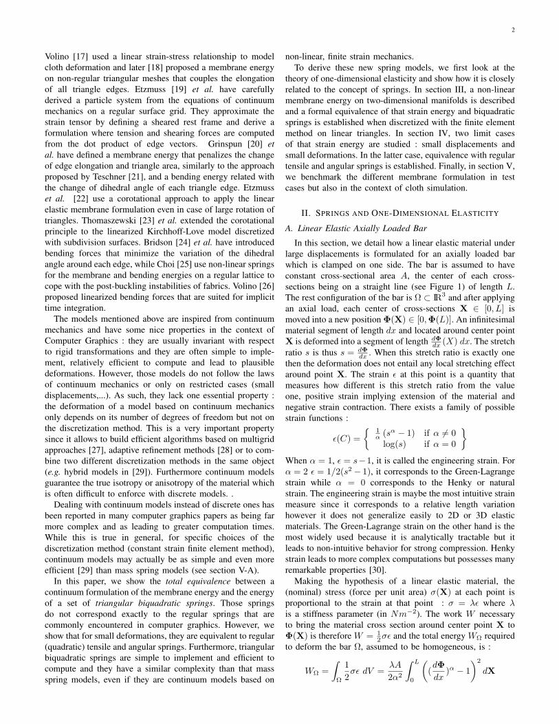
Fig. 1. Axially loaded bar in rest (top) and deformed (bottom) configurations.All cross sections are identical and of area A. The center line is a segment ofrest length L and is parameterized with function P (η) (resp. Q(η)), η ∈ [a, b]in its rest (resp. deformed) position.

If the segment [0, L] is parameterized by a function X =P (η), η ∈ [a, b] ⊂ IR and its deformation by a functionΦ(X) = Q(η), η ∈ [a, b] ⊂ IR then the deformation functioncan be written as : Φ(X) = Q(P−1(X)). In this case, thetotal energy WΩ can be expressed as :

WΩ =λA

2α2

∫ b

a

((dQ

dη)α − (

dP

dη)α

)2 (dP

dη

)(1−2α)

dη (1)

B. Stretching energy of deformable curves

Instead of studying the deformation of a straight bar, weconsider a curved bar Ω of cross-section A embedded ina Euclidean space IRd, d > 1. The center line curve pa-rameterized as P(η), is deformed into another curve Φ(Ω),parameterized with Q(η), η ∈ [a, b]. To obtain the stretchingenergy necessary to deform Ω into Φ(Ω), it suffices to replacein Equation 1 the first derivative dP

dη with the norm of the firstderivative ‖dP

dη ‖ :

WΩ =λA

2α2

∫ b

a

(‖dQ

dη‖α − ‖dP

dη‖α

)2 ∥∥∥∥dPdη

∥∥∥∥(1−2α)

dη (2)

If the parameter η is the arc length of the reference curve P(η)then the stretching energy simplifies as :

WΩ =λA

2α2

∫Ω

(‖dQ

dη‖α − 1

)2

dη (3)

Clearly, this functional is zero if the arc length of P(η) isalso the arc length of deformed curve Q(η)

C. Finite Element Discretization

We use in the remainder the Rayleigh-Ritz approach [31](p60) of the finite element method. This approach is equivalentto the Galerkin weighted residual method, and relies on thevariational form (strain energy) rather than the weak form(principle of virtual work) of the same elasticity problem.Dealing with the variational form is more convenient to derivesymmetric analytical expressions and is widely used in com-puter graphics. Equations are derived by first discretizing thestretching energy and then applying the principle of minimumpotential energy.

In Equation 2, the coordinate functions P(η) and Q(η) onlyneed to have their first derivative square integrable. Therefore,the reference curve Ω can be approximated with a set Ωh

of line segments Si : Ωh =⋃

i=1,..,N Si = [Pi,Pi+1].Each reference segment [Pi,Pi+1] is deformed into segment[Qi,Qi+1], the set of points Qi, i = 1, . . . , N being thenodes of the finite element model.

Ω Φ(Ω)

P(η)Q(η)

Pi Qi

Rest CurveDeformed Curve

hΩRest Polygon hΦ(Ω)Deformed Polygon

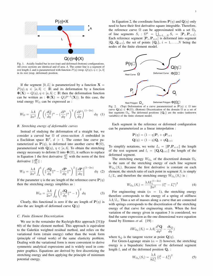
Fig. 2. (Top) Deformation of a curve parameterized as P(η) ∈ Ω intocurve Q(η) ∈ Φ(Ω); (Bottom) Discretization of the domain Ω as a set ofline segments Ωh. The deformed positions Qi are the nodes (unknownvariables) of the finite element model.

Each segment in the reference or deformed configurationcan be parameterized as a linear interpolation :

P(η) = (1− η)Pi + ηPi+1

Q(η) = (1− η)Qi + ηQi+1

To simplify notations, we write Li = ‖PiPi+1‖ the lengthof the rest segment and li = ‖QiQi+1‖ the length of thedeformed segment.

The stretching energy WΩhof the discretized domain Ωh

is the sum of the stretching energy of each line segmentWΩh

(Si). Because the first derivative is constant on eachelement, the stretch ratio of each point in segment Si is simplyli/Li and therefore the stretching energy WΩh

(Si) is :

WΩh(Si) =

λAL(1−2α)i

2α2(lαi − Lα

i )2 (4)

For engineering strain (α = 1), the stretching energytherefore corresponds to the energy of a spring of stiffnessλA/Li. Thus a set of masses along a curve that are connectedwith springs corresponds to the discretization of the stretchingenergy of that curve for engineering strain. When the firstvariation of the energy given in equation 3 is considered, wefind the same expression as the one dimensional wave equationfound by Etzmuss et al. [19] :

δWΩh(Si) = λA(

d2Qdη2

− dtQ

dη)

where tQ is the tangent vector at point Q(η).For Green-Lagrange strain (α = 2) however, the stretching

energy is a biquadratic function of the deformed segmentlength li and of the deformed position Qi :

WΩh(Si) =

λA

8L3i

(l2i − L2

i

)2(5)

4

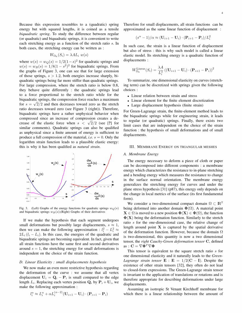
Because this expression resembles to a (quadratic) springenergy but with squared lengths, it is coined as a tensilebiquadratic spring. To study the difference between regular(or quadratic) and biquadratic springs, it is convenient to writeeach stretching energy as a function of the stretch ratio s. Inboth cases, the stretching energy can be written as :

WΩh(Si) = λALi w(s)

where w(s) = wQ(s) = 1/2(1−s)2 for quadratic springs andw(s) = wB(s) = 1/8(1− s2)2 for biquadratic springs. Fromthe graphs of Figure 3, one can see that for large extensionof those springs, s > 1.2, both energies increase sharply, bi-quadratic springs being far more stiffer than quadratic springs.For large compression, where the stretch ratio is below 0.8,they behave quite differently : the quadratic springs leadto a force proportional to the stretch ratio while for thebiquadratic springs, the compression force reaches a maximumfor s =

√2/2 and then decreases toward zero as the stretch

ratio decreases toward zero (see Figure 3 (right)). Therefore,biquadratic springs have a rather unphysical behavior whencompressed since an increase of compression creates a de-crease of the elastic force when s <

√2/2 (see [?] for

similar comments). Quadratic springs can also be qualifiedas unphysical since a finite amount of energy is sufficient toproduce a full compression of the material, i.e. s = 0. Only thelogarithm strain function leads to a plausible elastic energy:this is why it has been qualified as natural strain.

-0,15

0,05

0,25

0,45

0,65

0,85

1,05

1,25

-0,2 0,3 0,8 1,3 1,8

wQ(s)

wB(s)

s

-1,5

-1

-0,5

0

0,5

1

1,5

2

2,5

3

-0,2 0 0,2 0,4 0,6 0,8 1 1,2 1,4 1,6 1,8 2

dwQ

s

ds(s)

dwB

ds(s)

Fig. 3. (Left) Graphs of the energy functions for quadratic springs wQ(s)and biquadratic springs wB(s);(Right) Graphs of their derivatives

If we make the hypothesis that each segment undergoessmall deformations but possibly large displacements, s ≈ 1,then we can make the following approximation : l2i − L2

i ≈2Li (li − Li). In this case, the energies of the quadratic andbiquadratic springs are becoming equivalent. In fact, given thatall strain functions have the same first and second derivativesaround s = 1, the stretching energy for small deformations isindependent on the choice of the strain function.

D. Linear Elasticity : small displacements hypothesisWe now make an even more restrictive hypothesis regarding

the deformation of the curve : we assume that all vertexdisplacement Ui = Qi − Pi is small compared to the edgelength Li. Replacing each vertex position Qi by Pi +Ui, wemake the following approximation :

lαi ≈ Lαi + αL

(α−2)i (Ui+1 −Ui) · (Pi+1 −Pi)

Therefore for small displacements, all strain functions can beapproximated as the same linear function of displacement :

(sα − 1)/α ≈ (Ui+1 −Ui) · (Pi+1 −Pi)/L2i

In such case, the strain is a linear function of displacementbut also of stress : this is why such model is called a linearelastic model. Its stretching energy is a quadratic function ofdisplacements :

WLinearΩh

(Si) =λA

L3i

((Ui+1 −Ui) · (Pi+1 −Pi))2

To summarize, one dimensional elasticity on curves (stretch-ing term) can be discretized with springs given the followingchoices :

• Linear relation between strain and stress• Linear element for the finite element discretization• Large displacement hypothesis (finite strain)

For Green-Lagrange strain, the finite-element method leads tothe biquadratic springs while for engineering strain, it leadsto regular (or quadratic) springs. Finally, there exists twolimit cases that are independent on the choice of the strainfunction : the hypothesis of small deformations and of smalldisplacements.

III. MEMBRANE ENERGY ON TRIANGULAR MESHES

A. Membrane Energy

The energy necessary to deform a piece of cloth or papercan be decomposed into different components : a membraneenergy which characterizes the resistance to in-plane stretchingand a bending energy which measures the resistance to changein the surface normal orientation. The membrane energygeneralizes the stretching energy for curves and under theplane stress hypothesis [31] (p87), this energy only depends onthe change in local metrics of the surface (its first fundamentalform).

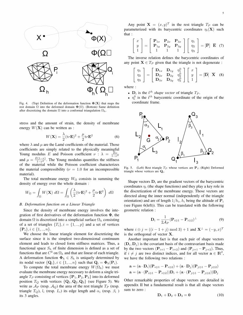
We consider a two-dimensional compact domain Ω ⊂ IR2

being deformed into another domain Φ(Ω). A material pointX ∈ Ω is moved to a new position Φ(X) ∈ Φ(Ω), the functionΦ(X) being the deformation function. Similarly to the stretchratio s for the one-dimensional case, the relative change oflength around point X is captured by the spatial derivativeof the deformation function. However, because the domain Ωis two-dimensional, this quantity is now a two dimensionaltensor, the right Cauchy-Green deformation tensor C, definedas : C = ∇ΦT∇Φ

This tensor is equivalent to the square stretch ratio s forone dimensional elasticity and it naturally leads to the Green-Lagrange strain tensor E : E = 1/2(C − I). Despite theexistence of other strain tensors [32], they often do not leadto closed-form expressions. The Green-Lagrange strain tensoris invariant to the application of translations or rotations and istherefore appropriate for describing deformations under largedisplacements.

Assuming an isotropic St Venant Kirchhoff membrane forwhich there is a linear relationship between the amount of

5

Ω Φ(Ω)

X Φ(X)

Ω Φ ( Ω )h hh

Pi Qi

Fig. 4. (Top) Definition of the deformation function Φ(X) that maps therest domain Ω into the deformed domain Φ(Ω). (Bottom) Same definitionafter discretizing the domain Ω into a conformal triangulation Ωh.

stress and the amount of strain, the density of membraneenergy W (X) can be written as :

W (X) =λ

2(trE)2 +

µ

2trE2 (6)

where λ and µ are the Lamé coefficients of the material. Thosecoefficients are simply related to the physically meaningfulYoung modulus E and Poisson coefficient ν : λ = Eν

1−ν2

and µ = E(1−ν)1−ν2 . The Young modulus quantifies the stiffness

of the material while the Poisson coefficient characterizesthe material compressibility (ν = 1.0 for an incompressiblematerial).

The total membrane energy WΩ consists in summing thedensity of energy over the whole domain :

WΩ =∫

Ω

W (X) dΩ =∫

Ω

(λ

2(trE)2 +

µ

2trE2

)dΩ

B. Deformation function on a Linear Triangle

Since the density of membrane energy involves the inte-gration of first derivatives of the deformation function Φ, thedomain Ω is discretized into a simplicial surface Ωh consistingof a set of triangles Ti, i = 1, .., p and a set of verticesPi, i ∈ 1, .., n.

We choose the linear triangle element for discretizing thesurface since it is the simplest two-dimensional continuumelement and leads to closed form stiffness matrices. Thus, afunctional space Sh of finite dimension is defined as a set offunctions that are C0 on Ωh and that are linear of each triangle.A deformation function Φh ∈ Sh is uniquely determined byits nodal vector Qi, i ∈ 1, .., n such that Qi = Φh(Pi).

To compute the total membrane energy W (Ωh) we mustevaluate the membrane energy necessary to deform a single tri-angle TP consisting of vertices P1,P2,P3 into its deformedposition TQ with vertices Q1,Q2,Q3 (see Figure 5). Wewrite as AP (resp. AQ) the area of the rest triangle TP (resp.triangle TQ), li (resp. Li) its edge length and αi (resp. βi )its 3 angles.

Any point X = (x, y)T in the rest triangle TP can beparameterized with its barycentric coordinates ηi(X) suchthat : x

y1

=

P1x P2x P3x

P1y P2y P3y

1 1 1

η1

η2

η3

= [P] E (7)

The inverse relation defines the barycentric coordinates ofany point X ∈ TP given that the triangle is not degenerate : η1

η2

η3

=

D1x D1y η01

D2x D2y η02

D3x D3y η03

xy1

= [D] X (8)

where :• Di is the ith shape vector of triangle TP .• η0

i is the ith barycentric coordinate of the origin of thecoordinate frame.

P1

2P

3P

l2

l3

L1

a1

a2

a3

2Q

1Q

3Q

L2

L

3

l 1G

b2b1

b3

Fig. 5. (Left) Rest triangle TP whose vertices are Pi; (Right) Deformedtriangle whose vertices are Qi.

Shape vectors Di are the gradient vectors of the barycentriccoordinates ηi (the shape functions) and they play a key role inthe discretization of the membrane energy. Those vectors aredirected along the inner normal (independently of the triangleorientation) and are of length 1/hi, hi being the altitude of Pi

(see Figure 6(left)). This can be translated with the followinggeometric relation :

Di =1

2AP(Pi⊕1 −Pi⊕2)⊥ (9)

where i ⊕ j = ((i − 1 + j) mod 3) + 1 and X⊥ = (−y, x)T

is the orthogonal of vector X.Another important fact is that each pair of shape vectors

(Di,Dj) is the covariant basis of the contravariant basis madeby the two vectors (Pi+1−Pi+2) and (Pj+1−Pj+2). Thus,if i 6= j are two distinct indices, and for all vector a ∈ IR2,we have the following two relations :

a = (a ·Di)(Pi⊕1 −Pi⊕2) + (a ·Dj)(Pj⊕1 −Pj⊕2)a = (a · (Pi⊕1 −Pi⊕2))Di + (a · (Pj⊕1 −Pj⊕2))Dj

Other remarkable properties of shape vectors are detailed inappendix II but a fundamental result is that all shape vectorssum to zero :

D1 + D2 + D3 = 0 (10)

6

P

2P

1

3

D2

D1

D3

P

2Q

1Q

3Q

J3

Cot b1Cot b2

J3*

Cot a1

Cot a2

Fig. 6. (Left) Shape vectors polarvi are orthogonal to each edge and directedinwards; (Right) The foot Ji is the barycenter of points Qj and Qk withcoefficients cot βj and cot βk while pseudo-foot point J?

i has barycentriccoordinates cot αj and cot αk .

To simplify notations, we introduce the centroid G oftriangle TP of barycentric coordinates ηi = 1/3 in theEquation 7 :

X =3∑

i=1

ηi(X) Pi =3∑

i=1

(13

+ Di · (X−G))

Pi (11)

The deformation function Φ(X) on a linear triangle maps apoint X ∈ TP such that Φ(X) has the same barycentriccoordinates in triangle TQ than X in triangle TP :

Φ(X) =3∑

i=1

ηi(X) Qi =3∑

i=1

(13

+ Di · (X−G))

Qi

(12)

C. Invariants of the Green-Lagrange Strain Tensor

To write the total membrane energy W (TP ) necessary todeform triangle TP into triangle TQ, it is necessary to write thetwo invariants trE and trE2 as a function of the two trianglesshape. From Equation 12, it can be seen that the gradient ofthe deformation function is independent is constant on the resttriangle TP which simplifies further expressions :

∇Φ =[∂Φi

∂xj

]=

3∑i=1

Qi ⊗Di

C = ∇ΦT∇Φ =3∑

i=1

3∑j=1

(Qi ·Qj)(Di ⊗Dj) (13)

The trace of the Green strain tensor trE is simply derivedfrom the trace of the tensor C : trE = 1/2(trC− 2). Fromequation 13, we easily get :

trC =3∑

i=1

3∑j=1

(Qi ·Qj)(Di ·Dj) (14)

Appendix III details how this sum of dot products can beexpressed as a function of edge length and angles. Theresulting expressions are simply :

trC =1

2AP

(l21 cot α1 + l22 cot α2 + l23 cot α3

)trE =

(l21 − L21) cot α1 + (l22 − L2

2) cot α2 + (l23 − L23) cot α3

2AP

The expression of trC is closely related to the Dirichletenergy used in discrete harmonic mapping [33]. Indeed, inthis case, the deformation Φ maps two planar surfaces andthe right Cauchy-Green deformation tensor is just the firstfundamental form and its trace the norm of the deformationmatrix : trC = ‖∇Φ‖2. Extending the analogy with the fieldof surface parametrization, we can see the membrane energyas a functional that enforces isometric mappings (instead ofconformal or harmonic ones) since it is minimal when C = I.

The second invariant of the strain tensor trE2 can be writtenas a function of the first invariant and the determinant of Ebut also of C :

trE2 = (trE)2 − 2 detE =1 + 2trE + 2(trE)2 − detC

2

The determinant of the deformation tensor C = ∇ΦT∇Φ isthe square of the determinant of Φ which is the ratio of thetwo triangle areas : detΦ = AQ/AP . Putting it all together,the second invariant is also a simple function of the squareedge elongation ∆2li = (l2i − L2

i )

trE2 =

∑i 6=j 2∆2li∆2lj −

∑3i=1(∆

2li)2

64A2P

D. Membrane Energy and Triangular Biquadratic Springs

The density of elastic energy W (X) is given by Equation6 and is constant for all points in triangle TP . Thus, fromprevious results, we can show that the total energy to deformtriangle TP into TQ is a function of square edge variation ∆2liand of the angles αi of the rest triangle :

WTRBS(TP ) =∫

TP

W (X) dX = AP W (G)

WTRBS(TP ) =3∑

i=1

(∆2li)2(2 cot2 αi(λ + µ) + µ)64AP

+ (15)

∑i 6=j

2∆2li∆2lj(2 cotαi cot αj(λ + µ)− µ)64AP

We call this formulation of the membrane energy the TRian-gular Biquadratic Springs (TRBS) since the first term can beinterpreted as the energy of three tensile biquadratic springsthat prevent edges from stretching while the second term canbe seen as three angular biquadratic springs that prevent anychange in vertex angles. We can thus rewrite the previousequation by enforcing the existence of those two types ofbiquadratic springs :

WTRBS(TP ) =3∑

i=1

kTPi

4(l2i − L2

i )2 +

∑i 6=j

cTP

k

2(l2i − L2

i )(l2j − L2

j )

where kTPand cTP

are the tensile and angular stiffness of thebiquadratic springs. Replacing the Lamé coefficients with theYoung modulus E and Poisson coefficient ν, we get :

kTPi =

2 cot2 αi(λ + µ) + µ

16AP=

E(2 cot2 αi + 1− ν)16(1− ν2)AP

cTP

k =2 cot αi cot αj(λ + µ)− µ

16AP=

E(2 cotαi cot αj + ν − 1)16(1− ν2)AP

7

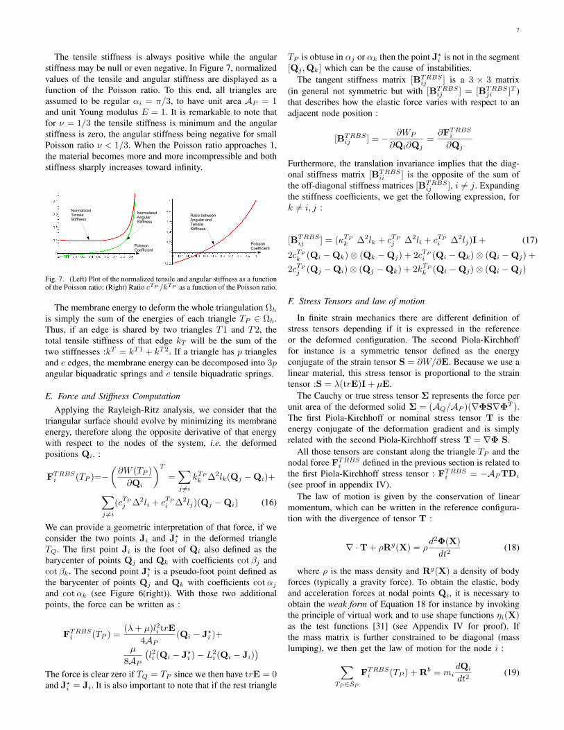
The tensile stiffness is always positive while the angularstiffness may be null or even negative. In Figure 7, normalizedvalues of the tensile and angular stiffness are displayed as afunction of the Poisson ratio. To this end, all triangles areassumed to be regular αi = π/3, to have unit area AP = 1and unit Young modulus E = 1. It is remarkable to note thatfor ν = 1/3 the tensile stiffness is minimum and the angularstiffness is zero, the angular stiffness being negative for smallPoisson ratio ν < 1/3. When the Poisson ratio approaches 1,the material becomes more and more incompressible and bothstiffness sharply increases toward infinity.

Poisson Coefficient

NormalizedTensile Stiffness

NormalizedAngular Stiffness

Poisson Coefficient

Ratio betweenAngular and Tensile Stiffness

Fig. 7. (Left) Plot of the normalized tensile and angular stiffness as a functionof the Poisson ratio; (Right) Ratio cTP /kTP as a function of the Poisson ratio.

The membrane energy to deform the whole triangulation Ωh

is simply the sum of the energies of each triangle TP ∈ Ωh.Thus, if an edge is shared by two triangles T1 and T2, thetotal tensile stiffness of that edge kT will be the sum of thetwo stiffnesses :kT = kT1 + kT2. If a triangle has p trianglesand e edges, the membrane energy can be decomposed into 3pangular biquadratic springs and e tensile biquadratic springs.

E. Force and Stiffness Computation

Applying the Rayleigh-Ritz analysis, we consider that thetriangular surface should evolve by minimizing its membraneenergy, therefore along the opposite derivative of that energywith respect to the nodes of the system, i.e. the deformedpositions Qi. :

FTRBSi (TP )=−

(∂W (TP )

∂Qi

)T

=∑j 6=i

kTP

k ∆2lk(Qj −Qi)+∑j 6=i

(cTPj ∆2li + cTP

i ∆2lj)(Qj −Qi) (16)

We can provide a geometric interpretation of that force, if weconsider the two points Ji and J?

i in the deformed triangleTQ. The first point Ji is the foot of Qi also defined as thebarycenter of points Qj and Qk with coefficients cot βj andcot βk. The second point J?

i is a pseudo-foot point defined asthe barycenter of points Qj and Qk with coefficients cot αj

and cot αk (see Figure 6(right)). With those two additionalpoints, the force can be written as :

FTRBSi (TP ) =

(λ + µ)l2i trE4AP

(Qi − J?i )+

µ

8AP

(l2i (Qi − J?

i )− L2i (Qi − Ji)

)The force is clear zero if TQ = TP since we then have trE = 0and J?

i = Ji. It is also important to note that if the rest triangle

TP is obtuse in αj or αk then the point J?i is not in the segment

[Qj ,Qk] which can be the cause of instabilities.The tangent stiffness matrix [BTRBS

ij ] is a 3 × 3 matrix(in general not symmetric but with [BTRBS

ij ] = [BTRBSji ]T )

that describes how the elastic force varies with respect to anadjacent node position :

[BTRBSij ] = − ∂WP

∂Qi∂Qj=

∂FTRBSi

∂Qj

Furthermore, the translation invariance implies that the diag-onal stiffness matrix [BTRBS

ii ] is the opposite of the sum ofthe off-diagonal stiffness matrices [BTRBS

ij ], i 6= j. Expandingthe stiffness coefficients, we get the following expression, fork 6= i, j :

[BTRBSij ] = (κTP

k ∆2lk + cTPj ∆2li + cTP

i ∆2lj)I + (17)

2cTP

k (Qi −Qk)⊗ (Qk −Qj) + 2cTPi (Qi −Qk)⊗ (Qi −Qj) +

2cTPj (Qj −Qi)⊗ (Qj −Qk) + 2kTP

k (Qi −Qj)⊗ (Qi −Qj)

F. Stress Tensors and law of motion

In finite strain mechanics there are different definition ofstress tensors depending if it is expressed in the referenceor the deformed configuration. The second Piola-Kirchhofffor instance is a symmetric tensor defined as the energyconjugate of the strain tensor S = ∂W/∂E. Because we use alinear material, this stress tensor is proportional to the straintensor :S = λ(trE)I + µE.

The Cauchy or true stress tensor Σ represents the force perunit area of the deformed solid Σ = (AQ/AP )(∇ΦS∇ΦT ).The first Piola-Kirchhoff or nominal stress tensor T is theenergy conjugate of the deformation gradient and is simplyrelated with the second Piola-Kirchhoff stress T = ∇Φ S.

All those tensors are constant along the triangle TP and thenodal force FTRBS

i defined in the previous section is related tothe first Piola-Kirchhoff stress tensor : FTRBS

i = −AP TDi

(see proof in appendix IV).The law of motion is given by the conservation of linear

momentum, which can be written in the reference configura-tion with the divergence of tensor T :

∇ ·T + ρRg(X) = ρd2Φ(X)

dt2(18)

where ρ is the mass density and Rg(X) a density of bodyforces (typically a gravity force). To obtain the elastic, bodyand acceleration forces at nodal points Qi, it is necessary toobtain the weak form of Equation 18 for instance by invokingthe principle of virtual work and to use shape functions ηi(X)as the test functions [31] (see Appendix IV for proof). Ifthe mass matrix is further constrained to be diagonal (masslumping), we then get the law of motion for the node i :∑

TP∈SP

FTRBSi (TP ) + Rb = mi

dQi

dt2(19)

8

IV. APPROXIMATION OF THE MEMBRANE ENERGY

A. Small Displacements : Linear Elastic Membrane

We propose a first approximation of the membrane energyin the case of small displacements, corresponding to theframework of linear elasticity. In such case, it is preferableto analyze the deformation of a membrane surface in termsof displacement u(X) = Φ(X) − X rather than in termsof deformation Φ(X). The linear elastic membrane energyis derived by replacing the Green-Lagrange strain tensor withits linearized version : EL = 1

2 (∇u +∇uT ).On a linear triangle element, the linear membrane energy is

a quadratic expression of the displacements ui of the threevertices (see [6] for an equivalent expression of the localstiffness matrix) :

WL(TP ) =12

3∑i,j=0

uTi [BL

ij ]uj

[BLij ] =

[λ(Di ⊗Dj) +

µ

2(Dj ⊗Di) +

µ

2(Di ·Dj)I

]The linear elastic approximation is advantageous in terms

of computational efficiency (see section V-A) since the elasticforce can be evaluated by a simple matrix vector compu-tation which is why it has been coined as a Tensor-Massapproach [29]. However it is quite restrictive in practice withthe occurrence of exaggerated dilation when large rotationsare applied [34]. Note that when Qi = Pi, the TRBS tangentstiffness matrix of Equation 17 is equal to the linear elasticstiffness matrix.

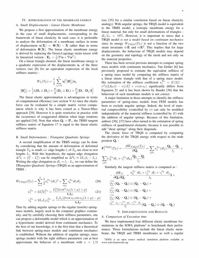
B. Small Deformations : Triangular Quadratic Springs

A second simplification of the TRBS energy can be doneby considering that the amount of deformation of deformedtriangle TQ is small, i.e. edge lengths li of TQ are close to restlengths Li. With this hypothesis, the square edge elongation∆2li = (l2i − L2

i ) can be simplified as ∆2li ≈ 2Li(li − Li).Writing the edge elongation as dli = li−Li, we can define theTRiangular Quadratic Springs (TRQS) as an approximation ofTRBS :

WTRQS(TP ) =3∑

i=1

12κTP

i (dli)2 +∑i 6=j

γTP

k dlidlj (20)

κTPi = 2L2

i kTPi =

L2i (2 cot2 αi(λ + µ) + µ)

8AP(21)

γTP

k = 2LiLjcTP

k =LiLj(2 cotαi cot αj(λ + µ)− µ)

8AP

Thus by adding angular springs to the regular (tensile) spring-mass models, largely used in the computer graphics commu-nity, and by carefully choosing their stiffness parameters, onecan propose a deformable model which is an approximation ofa hyperelastic model derived from continuum mechanics. Tothe best of our knowledge, it is the first time that a theoreticallink between spring-mass models and continuum mechanicsis established. Without the addition of angular springs, masssprings models with the right stiffness parameters can at bestapproximate the behavior of a membrane with ν = 1/3

(see [35] for a similar conclusion based on linear elasticityanalogy). With angular springs, the TRQS model is equivalentto the TRBS model, a isotropic membrane energy for alinear material, but only for small deformations of triangles :dli/Li < 10%. However, it is important to stress that aTRQS model is not a model based on continuum mechanicssince its energy WTRQS(TP ) is not a function of the twostrain invariants trE and trE2. This implies that for largedisplacements, the behaviour of TRQS models may dependon the geometry and topology of the mesh and not only onthe material properties.

There has been several previous attempts to compare springmass models with continuum mechanics. Van Gelder [6] haspreviously proposed to estimate the equivalent stiffness ofa spring mass model by comparing the stiffness matrix ofa linear elastic triangle with that of a spring mass model.His estimation of the stiffness coefficient κTP

i = E/2(1 −ν2)(2AP (1 − ν)/L2

i + ν cot αi) significantly differs fromEquation 21 and it has been shown by Baudet [36] that thebehaviour of such membrane models is not correct.

A major limitation in those attempts to identify the stiffnessparameters of spring-mass models from FEM models hasbeen to exclude angular springs. Indeed, the level of mate-rial compressibility (controlled by ν) can only be modifiedindependently of the material stiffness (controlled by E) withthe addition of angular springs. Because of this limitation,authors [36], [37] have often turned to the estimation of springstiffness of quadrilateral elements, because it was possible toadd "shear springs" along their diagonals.

The elastic force of TRQS is computed by computingthe derivative of the TRQS energy with respect to the nodeposition Qi :

FTRQSi (TP ) = −∂WTRQS(TP )

∂Qi=

∑j 6=i

κTPj (dlj)

Qk −Qi

lj+

∑j 6=i

(γTP

k dli + γTPi dlk)

Qk −Qi

lj

Similarly the tangent stiffness matrix is computed as :

− ∂WP

∂Qi∂Qj=

κTP

k dlk + γTPj dli + γTP

i dlj

lkI +

γTPk

lilj(Qk −Qi)⊗ (Qj −Qk) +

γTPi

lj lk(Qi −Qk)⊗ (Qi −Qj) +

γTPj

lilk(Qj −Qi)⊗ (Qj −Qk) +

κTPk Lk−γ

TPj dli−γ

TPi dlj

l3k(Qi −Qj)⊗ (Qi −Qj)

V. IMPLEMENTATION AND RESULTS

A. Comparison of Execution timeWe have implemented four different elastic membrane for-

mulations in the SOFA platform1 to benchmark their perfor-mance. Those formulations include the linear elastic mem-brane, the TRQS and TRBS membranes as well a regular

1SOFA is an open source medical simulation platform available atwww.sofa-framework.org

9

spring-mass membrane obtained by dropping the angularsprings in the TRQS formulation.

To optimize the execution time of the TRBS and TRQSmembrane forces, the tensile stiffness κTP

i and kTPi are stored

on edges and are accumulated from adjacent triangles. Thus,the force computation first requires to examine all edges tocompute their extensions (∆2li and dli) and the tensile termsfollowed by the examination of all triangles to add the angularterms. In the latter case, each edge term may be computedonly once by taking advantage of the action-reaction principle(Fi→j = −Fj→i).

In section III-F we have showed that the application of theregular finite element or finite volume method (such as [38])is equivalent to the TRBS membrane but with a formulationof the force which involves the first Piola-Kirchhoff ten-sor :FTRBS

i = −AP TDi. The computation of the membraneforces for the three vertices of a tridimensional triangle basedon FEM requires 121 multiplications and 75 additions whilethe TRBS forces can be computed with 30 multiplications and44 additions2 which represents at least a speedup factor of two.Thus, the biquadratic spring formulation performs an optimalassembly of the stiffness information.

0

0,02

0,04

0,06

0,08

0,1

0,12

0,14

TRQS TRBS Springs Linear

seco

nd

Force Computation DfDx Computation

Fig. 8. Execution times to compute 100 times the elastic force Fi and thematrix-vector product [Bij ]X for 4 differents elastic membrane formulations.

In Figure 8, we compare the execution times for theevaluation of the elastic membrane force Fi as well as thematrix-vector product [Bij ]X on a triangular mesh having774 vertices and 1546 triangles. The matrix-vector productevaluation is useful to benchmark the performance of theconjugated gradient algorithm. The linear elastic membraneis the most efficient, followed by the spring-mass, TRBSand TRQS models. The TRBS is only 60% more expensivethan the spring-mass, while the TRBS is itself 60 % moreexpensive than the TRQS. The execution times for the matrix-vector products follow the same hierarchy but with smallerdifferences between the models (the TRQS is only 20% moreexpensive than the TRBS in this case).

2The decomposition of forces based on FEM exploits the fact that all nodalforces of a triangle sum to zero Fi + Fj + Fk = 0. In the case of TRBS,we have assumed that each edge is shared by two triangles.

B. Comparison on test cases

We compare the behavior of the four membrane formu-lations in a pure traction study for which there is a knownanalytical solution for linear elastic materials. Figure 9 summa-rizes the boundary conditions consisting in applying a knownpressure p on the top of a square membrane while preventingthe vertical displacements of the bottom vertices. In the linearelastic case, the vertical and horizontal strains, εy and εx

are proportional to the applied pressure : εy = E p andεx = E ν p.

No vertical displacements

Constant Vertical Pressure p

Dx Dy

h

L

Fig. 9. Pure traction experiment where a constant pressure is applied on aslab, bottom vertices being constrained to have zero vertical displacements.The horizontal and vertical deformations are computed as εx = Dx/L andεy = Dy/h.

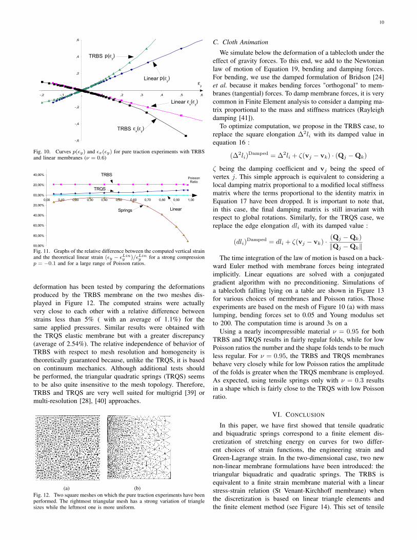
Several indentation tests have been performed on a mem-brane material having unit Young Modulus E = 1 and varyingPoisson ratios ν ∈ [0, 1[. We solve those non-linear staticproblems with an implicit method, using the tangent stiffnessmatrices (Newton-Raphson algorithm), each linear system ofequations being solved with the modified conjugated gradientof Baraff and Witkin [14]. In Figure 10, the curves p(εy) ≈Eεy and εx(εy) ≈ −νεy are displayed for the linear and theTRBS membranes for a given Poisson ratio ν = 0.6. Thosecurves have been computed from the mesh of Figure 12 (a). Asexpected, all curves are linear for small strains while the TRBSmembrane leaves the domain of linearity for strain greater than3%. For extensions, p > 0, TRBS membranes exhibit a greaterstiffness than linear membranes while the converse is true forcompressions. The differences in the stress-strain relationshipscan be readily explained by the difference between the Green-Lagrange strain (quadratic function of stretch) used in theTRBS model and the engineering strain (linear function ofstretch) for the linear model. Indeed, the curves p(εy) closelyresemble that of the curves dwB/ds in Figure 3.

For a strong compression, p = −0.1, away from the lineardomain εx ≈ 10%, the TRBS membrane exhibits verticalstrains that are on average 20% greater than in the linearcase (see Figure 11). The TRQS membrane has a intermediatebehavior between the linear and TRBS membranes which issensible since it is a large displacement formulation (as theTRBS case) but with a strain measure (engineering strain)similar to linear materials. Finally using tensile springs leadsto solutions that are far from being physical except when thePoisson ratio is close to 0.3, which correlates the findings ofsection III-D.

The impact of the mesh homogeneity on the computed

10

TRBS p(ey)

Linear p(ey)

TRBS ex(ey)

Linear ex(ey)

ey

-,6

-,4

-,2

,

,2

,4

,6

-,2 -,1 , ,1 ,2 ,3 ,4 ,5 ,6

Fig. 10. Curves p(εy) and εx(εy) for pure traction experiments with TRBSand linear membranes (ν = 0.6)

-100,00%

-80,00%

-60,00%

-40,00%

-20,00%

00,00%

20,00%

40,00%

0,00 0,10 0,20 0,30 0,40 0,50 0,60 0,70 0,80 0,90 1,00

PoissonRatio

TRBS

TRQS

Springs Linear

Fig. 11. Graphs of the relative difference between the computed vertical strainand the theoretical linear strain (εy − εLin

y )/εLiny for a strong compression

p = −0.1 and for a large range of Poisson ratios.

deformation has been tested by comparing the deformationsproduced by the TRBS membrane on the two meshes dis-played in Figure 12. The computed strains were actuallyvery close to each other with a relative difference betweenstrains less than 5% ( with an average of 1.1%) for thesame applied pressures. Similar results were obtained withthe TRQS elastic membrane but with a greater discrepancy(average of 2.54%). The relative independence of behavior ofTRBS with respect to mesh resolution and homogeneity istheoretically guaranteed because, unlike the TRQS, it is basedon continuum mechanics. Although additional tests shouldbe performed, the triangular quadratic springs (TRQS) seemsto be also quite insensitive to the mesh topology. Therefore,TRBS and TRQS are very well suited for multigrid [39] ormulti-resolution [28], [40] approaches.

(a) (b)Fig. 12. Two square meshes on which the pure traction experiments have beenperformed. The rightmost triangular mesh has a strong variation of trianglesizes while the leftmost one is more uniform.

C. Cloth Animation

We simulate below the deformation of a tablecloth under theeffect of gravity forces. To this end, we add to the Newtonianlaw of motion of Equation 19, bending and damping forces.For bending, we use the damped formulation of Bridson [24]et al. because it makes bending forces "orthogonal" to mem-branes (tangential) forces. To damp membrane forces, it is verycommon in Finite Element analysis to consider a damping ma-trix proportional to the mass and stiffness matrices (Rayleighdamping [41]).

To optimize computation, we propose in the TRBS case, toreplace the square elongation ∆2li with its damped value inequation 16 :

(∆2li)Damped = ∆2li + ζ(vj − vk) · (Qj −Qk)

ζ being the damping coefficient and vj being the speed ofvertex j. This simple approach is equivalent to considering alocal damping matrix proportional to a modified local stiffnessmatrix where the terms proportional to the identity matrix inEquation 17 have been dropped. It is important to note that,in this case, the final damping matrix is still invariant withrespect to global rotations. Similarly, for the TRQS case, wereplace the edge elongation dli with its damped value :

(dli)Damped = dli + ζ(vj − vk) · (Qj −Qk)‖Qj −Qk‖

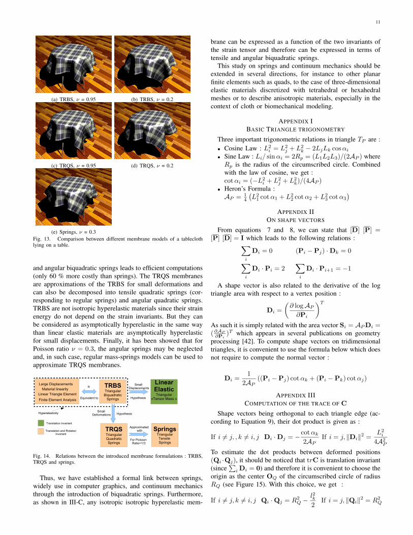
The time integration of the law of motion is based on a back-ward Euler method with membrane forces being integratedimplicitly. Linear equations are solved with a conjugatedgradient algorithm with no preconditioning. Simulations ofa tablecloth falling lying on a table are shown in Figure 13for various choices of membranes and Poisson ratios. Thoseexperiments are based on the mesh of Figure 10 (a) with masslumping, bending forces set to 0.05 and Young modulus setto 200. The computation time is around 3s on a

Using a nearly incompressible material ν = 0.95 for bothTRBS and TRQS results in fairly regular folds, while for lowPoisson ratios the number and the shape folds tends to be muchless regular. For ν = 0.95, the TRBS and TRQS membranesbehave very closely while for low Poisson ratios the amplitudeof the folds is greater when the TRQS membrane is employed.As expected, using tensile springs only with ν = 0.3 resultsin a shape which is fairly close to the TRQS with low Poissonratio.

VI. CONCLUSION

In this paper, we have first showed that tensile quadraticand biquadratic springs correspond to a finite element dis-cretization of stretching energy on curves for two differ-ent choices of strain functions, the engineering strain andGreen-Lagrange strain. In the two-dimensional case, two newnon-linear membrane formulations have been introduced: thetriangular biquadratic and quadratic springs. The TRBS isequivalent to a finite strain membrane material with a linearstress-strain relation (St Venant-Kirchhoff membrane) whenthe discretization is based on linear triangle elements andthe finite element method (see Figure 14). This set of tensile

11

(a) TRBS, ν = 0.95 (b) TRBS, ν = 0.2

(c) TRQS, ν = 0.95 (d) TRQS, ν = 0.2

(e) Springs, ν = 0.3Fig. 13. Comparison between different membrane models of a tableclothlying on a table.

and angular biquadratic springs leads to efficient computations(only 60 % more costly than springs). The TRQS membranesare approximations of the TRBS for small deformations andcan also be decomposed into tensile quadratic springs (cor-responding to regular springs) and angular quadratic springs.TRBS are not isotropic hyperelastic materials since their strainenergy do not depend on the strain invariants. But they canbe considered as asymptotically hyperelastic in the same waythan linear elastic materials are asymptotically hyperelasticfor small displacements. Finally, it has been showed that forPoisson ratio ν = 0.3, the angular springs may be neglectedand, in such case, regular mass-springs models can be used toapproximate TRQS membranes.

Large DisplacementsMaterial linearity

Linear Triangle ElementFinite Element Analysis

TRBSTriangularBiquadratic

Springs

is

Equivalent to

Small Displacements

Hypothesis

LinearElasticTriangular

«Tensor Mass »

Small Deformations Hypothesis

TRQSTriangularQuadraticSprings

For Poisson Ratio=1/3

Approximated with Springs

TriangularTensile Springs

Translation Invariant

Translation and RotationInvariant

Hyperelasticity

Fig. 14. Relations between the introduced membrane formulations : TRBS,TRQS and springs.

Thus, we have established a formal link between springs,widely use in computer graphics, and continuum mechanicsthrough the introduction of biquadratic springs. Furthermore,as shown in III-C, any isotropic isotropic hyperelastic mem-

brane can be expressed as a function of the two invariants ofthe strain tensor and therefore can be expressed in terms oftensile and angular biquadratic springs.

This study on springs and continuum mechanics should beextended in several directions, for instance to other planarfinite elements such as quads, to the case of three-dimensionalelastic materials discretized with tetrahedral or hexahedralmeshes or to describe anisotropic materials, especially in thecontext of cloth or biomechanical modeling.

APPENDIX IBASIC TRIANGLE TRIGONOMETRY

Three important trigonometric relations in triangle TP are :• Cosine Law : L2

i = L2j + L2

k − 2LjLk cos αi

• Sine Law : Li/ sinαi = 2Rp = (L1L2L3)/(2AP ) whereRp is the radius of the circumscribed circle. Combinedwith the law of cosine, we get :cot αi = (−L2

i + L2j + L2

k)/(4AP )• Heron’s Formula :AP = 1

4

(L2

1 cot α1 + L22 cot α2 + L2

3 cot α3

)APPENDIX II

ON SHAPE VECTORS

From equations 7 and 8, we can state that [D] [P] =[P] [D] = I which leads to the following relations :∑

i

Di = 0 (Pi −Pj) ·Dk = 0∑i

Di ·Pi = 2∑

i

Di ·Pi+1 = −1

A shape vector is also related to the derivative of the logtriangle area with respect to a vertex position :

Di =(

∂ logAP

∂Pi

)T

As such it is simply related with the area vector Si = AP Di =(∂AP

∂Pi)T which appears in several publications on geometry

processing [42]. To compute shape vectors on tridimensionaltriangles, it is convenient to use the formula below which doesnot require to compute the normal vector :

Di =1

2AP((Pi −Pj) cot αk + (Pi −Pk) cot αj)

APPENDIX IIICOMPUTATION OF THE TRACE OF C

Shape vectors being orthogonal to each triangle edge (ac-cording to Equation 9), their dot product is given as :

If i 6= j, , k 6= i, j Di ·Dj = −cot αk

2APIf i = j, ‖Di‖2 =

L2i

4A2P

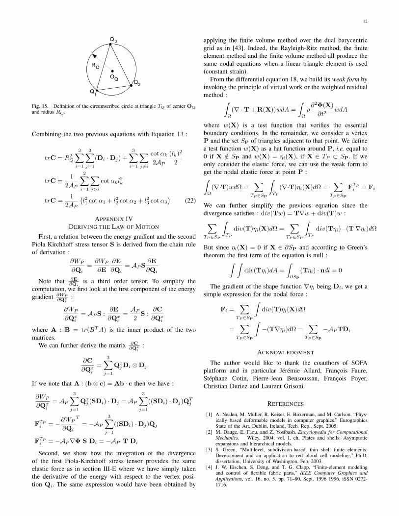
To estimate the dot products between deformed positions(Qi ·Qj), it should be noticed that trC is translation invariant(since

∑i Di = 0) and therefore it is convenient to choose the

origin as the center OQ of the circumscribed circle of radiusRQ (see Figure 15). With this choice, we get :

If i 6= j, k 6= i, j Qi ·Qj = R2Q −

l2k2

If i = j, ‖Qi‖2 = R2Q

12

2Q

1Q

3Q

RQ

OQ

Fig. 15. Definition of the circumscribed circle at triangle TQ of center OQ

and radius RQ.

Combining the two previous equations with Equation 13 :

trC = R2Q

3∑i=1

3∑j=1

(Di ·Dj) +3∑

i=1

∑j 6=i

cot αk

2AP

(lk)2

2

trC =1

2AP

2∑i=1

∑j>i

cot αkl2k

trC =1

2AP

(l21 cot α1 + l22 cot α2 + l23 cot α3

)(22)

APPENDIX IVDERIVING THE LAW OF MOTION

First, a relation between the energy gradient and the secondPiola Kirchhoff stress tensor S is derived from the chain ruleof derivation :

∂WP

∂Qi=

∂WP

∂E∂E∂Qi

= AP S∂E∂Qi

Note that ∂E∂Qi

is a third order tensor. To simplify thecomputation, we first look at the first component of the energygradient ∂WP

∂Qxi

:

∂WP

∂Qxi

= AP S :∂E∂Qx

i

=AP

2S :

∂C∂Qx

i

where A : B = tr(BT A) is the inner product of the twomatrices.

We can further derive the matrix ∂C∂Qx

i:

∂C∂Qx

i

=3∑

j=1

Qxj Di ⊗Dj

If we note that A : (b⊗ c) = Ab · c then we have :

∂WP

∂Qxi

= AP

3∑j=1

Qxj (SDi) ·Dj = AP

3∑j=1

((SDi) ·Dj)QTj

FTPi = −∂WP

∂Qi

T

= −AP

3∑j=1

((SDi) ·Dj)Qj

FTPi = −AP∇Φ S Di = −AP T Di

Second, we show how the integration of the divergenceof the first Piola-Kirchhoff stress tensor provides the sameelastic force as in section III-E where we have simply takenthe derivative of the energy with respect to the vertex posi-tion Qi. The same expression would have been obtained by

applying the finite volume method over the dual barycentricgrid as in [43]. Indeed, the Rayleigh-Ritz method, the finiteelement method and the finite volume method all produce thesame nodal equations when a linear triangle element is used(constant strain).

From the differential equation 18, we build its weak form byinvoking the principle of virtual work or the weighted residualmethod :∫

Ω

(∇ ·T + R(X))wdA =∫

Ω

ρ∂2Φ(X)

∂t2wdA

where w(X) is a test function that verifies the essentialboundary conditions. In the remainder, we consider a vertexP and the set SP of triangles adjacent to that point. We definea test function w(X) as a hat function around P, i.e. equal to0 if X /∈ SP and w(X) = ηi(X), if X ∈ TP ⊂ SP. If weonly consider the elastic force, we can use the weak form toget the nodal elastic force at point P :∫

Ω

(∇·T)wdΩ =∑

TP∈SP

∫TP

(∇·T)ηi(X)dΩ =∑

TP∈SP

FTPi = Fi

We can further simplify the previous equation since thedivergence satisfies : div(Tw) = T∇w + div(T)w :∑TP∈SP

∫TP

div(T)ηi(X)dΩ =∑

TP∈SP

∫TP

div(Tηi)−(T∇ηi)dΩ

But since ηi(X) = 0 if X ∈ ∂SP and according to Green’stheorem the first term of the equation is null :∫ ∫

div(Tηi)dA =∫

∂SP

(Tηi) · ndl = 0

The gradient of the shape function ∇ηi being Di, we get asimple expression for the nodal force :

Fi =∑

TP∈SP

∫div(T)ηi(X)dΩ

=∑

TP∈SP

∫−(T∇ηi)dΩ =

∑TP∈SP

−AP TDi

ACKNOWLEDGMENT

The author would like to thank the coauthors of SOFAplatform and in particular Jérémie Allard, François Faure,Stéphane Cotin, Pierre-Jean Bensoussan, François Poyer,Christian Duriez and Laurent Grisoni.

REFERENCES

[1] A. Nealen, M. Muller, R. Keiser, E. Boxerman, and M. Carlson, “Phys-ically based deformable models in computer graphics.” EurographicsState of the Art, Dublin, Ireland, Tech. Rep., Sept. 2005.

[2] M. Dauge, E. Faou, and Z. Yosibash, Encyclopedia for ComputationalMechanics. Wiley, 2004, vol. I, ch. Plates and shells: Asymptoticexpansions and hierarchical models.

[3] S. Green, “Multilevel, subdivision-based, thin shell finite elements:Development and an application to red blood cell modeling,” Ph.D.dissertation, University of Washington, Feb. 2003.

[4] J. W. Eischen, S. Deng, and T. G. Clapp, “Finite-element modelingand control of flexible fabric parts,” IEEE Computer Graphics andApplications, vol. 16, no. 5, pp. 71–80, Sept. 1996 1996, iSSN 0272-1716.

13

[5] F. Cirak, M. Ortiz, and P. Schröder, “Subdivision surfaces: new paradigmfor thin-shell finite-element analysis,” International Journal for Numer-ical Methods in Engineering, vol. 47, no. 12, p. 2039U2072, 2000.

[6] A. Van Gelder, “Approximate simulation of elastic membranes bytriangulated spring meshes,” Journal of Graphics Tools: JGT, vol. 3,no. 2, pp. 21–41, 1998.

[7] G. Bianchi, B. Solenthaler, G. Székely, and M. Harders, “Simultaneoustopology and stiffness identification for mass-spring models basedon fem reference deformations,” in Medical Image Computing andComputer-Assisted Intervention MICCAI 2004, C. Barillot, Ed., vol. 2.Springer, November 2004, pp. 293–301.

[8] J. Louchet, X. Provot, and D. Crochemore, “Evolutionary identificationof cloth animation models,” in Computer Animation and Simulation ’95,D. Terzopoulos and D. Thalmann, Eds., Eurographics. Springer-Verlag,Sept. 1995, pp. 44–54.

[9] D. Terzopoulos, J. Platt, A. Barr, and K. Fleischer, “Elastically de-formable models,” in Computer Graphics (SIGGRAPH-87), vol. 21,no. 3, 1987, pp. 205–214.

[10] K. Waters and D. Terzopoulos, “Modeling and animating faces usingscanned data,” The Journal of Visualization and Computer Animation,vol. 2, pp. 129–131, 1991.

[11] A. Maciel, R. Boulic, and D. Thalmann, “Deformable tissue parameter-ized by properties of real biological tissue,” in International Symposiumon Surgery Simulation and Soft Tissue Modeling (IS4TM’03), vol. 2673.Springer-Verlag Heidelberg, 2003, pp. 74–87.

[12] X. Provot, “Deformation constraints in a mass–spring model to describerigid cloth behavior,” in Graphics Interface ’95, May 1995, pp. 147–154.

[13] D. E. Breen, D. H. House, and M. J. Wozny, “Predicting the drape ofwoven cloth using interacting particles,” in Proceedings of SIGGRAPH’94 (Orlando, Florida, July 24–29, 1994), ser. Computer GraphicsProceedings, Annual Conference Series, A. Glassner, Ed., ACM SIG-GRAPH. ACM Press, July 1994, pp. 365–372.

[14] D. Baraff and A. Witkin, “Large steps in cloth simulation,” in ComputerGraphics (SIGGRAPH’98), ACM, Ed., Orlando (USA), July 1998, pp.43–54.

[15] J. Eischen and R. Bigliani, Cloth Modeling and Animation. A.K. Peters,2000, ch. Continuum versus particle representations, pp. 19–122.

[16] D. Bourguignon and M.-P. Cani, “Controlling anisotropy in mass-springsystems,” in Computer Animation and Simulation ’00, ser. Eurographics,N. Magnenat-Thalmann, D. Thalmann, and B. Arnaldi, Eds. Springer-Verlag Wien New York, 2000, pp. 113–123, proceedings of the Euro-graphics Workshop in Interlaken, Switzerland, August 21–22, 2000.

[17] P. Volino, M. Courchesne, and N. M. Thalmann, “Versatile andefficient techniques for simulating cloth and other deformableobjects,” Computer Graphics, vol. 29, no. Annual Conference Series,pp. 137–144, Nov. 1995. [Online]. Available: http://www.acm.org:80/pubs/citations/proceedings/graph/218380/p137-volino/

[18] P. Volino and N. Magnenat-Thalmann, “Developing simulation tech-niques for an interactive clothing system,” in Proceedings of Inter-national Conference on Virtual Systems and MultiMedia. Geneva,Switzerland: IEEE, 1997, pp. 109–118.

[19] O. Etzmuss, J. Gross, and W. Strasser, “Deriving a particlesystem from continuum mechanics for the animation ofdeformable objects,” IEEE Transactions on Visualization andComputer Graphics, vol. 9, no. 4, pp. 538–550, Oct./Dec.2003. [Online]. Available: http://csdl.computer.org/comp/trans/tg/2003/04/v0538abs.htm;http://csdl.computer.org/dl/trans/tg/2003/04/v0538.pdf

[20] E. Grinspun, A. N. Hirani, M. Desbrun, and P. Schröder,“Discrete shells,” in Eurographics/SIGGRAPH Symposium on ComputerAnimation, D. Breen and M. Lin, Eds. San Diego, California:Eurographics Association, 2003, pp. 62–67. [Online]. Available:http://www.eg.org/EG/DL/WS/SCA03/062-067.pdf

[21] M. Teschner, B. Heidelberger, M. Mueller, and M. Gross, “A versatileand robust model for geometrically complex deformable solids,” inComputer Graphics International CGI’04, Crete, Greece, 2004, pp. 312–319.

[22] O. Etzmuss, M. Keckeisen, and W. Straßer, “A Fast Finite ElementSolution for Cloth Modelling,” in Proceedings of Pacific Graphics,Canmore, Canada, 2003, pp. 244–252.

[23] B. Thomaszewski, M. Wacker, and W. Straßer, “A consistent bendingmodel for cloth simulation with corotational subdivision finite elements,”in Proceedings of ACM SIGGRAPH/Eurographics Symposium on Com-puter Animation (SCA 2006). ACM Press, 2006, pp. 0–10.

[24] R. Bridson, S. Marino, and R. Fedkiw, “Simulation of clothingwith folds and wrinkles,” in Eurographics/SIGGRAPH Symposiumon Computer Animation, D. Breen and M. Lin, Eds. San Diego,

California: Eurographics Association, 2003, pp. 28–36. [Online].Available: http://www.eg.org/EG/DL/WS/SCA03/028-036.pdf

[25] K.-J. Choi and H.-S. Ko, “Stable but responsive cloth,” in SIGGRAPH2002 Conference Proceedings, ser. Annual Conference Series, J. Hughes,Ed. ACM Press/ACM SIGGRAPH, 2002, pp. 604–611. [Online].Available: http://visinfo.zib.de/EVlib/Show?EVL-2002-209

[26] P. Volino and N. Magnenat-Thalmann, “Simple linear bending stiffnessin particle systems,” in Symposium on Computer Animation. Euro-graphics/ACM.

[27] W. L. Briggs, V. E. Henson, and S. F. McCormick, A Multigrid Tutorial,second edition ed. The Society for Industrial and Applied Mathematics(SIAM), 2000.

[28] E. Grinspun, P. Krysl, and P. Schröder, “CHARMS: a simple frameworkfor adaptive simulation,” ACM Transactions on Graphics, vol. 21, no. 3,pp. 281–290, July 2002.

[29] S. Cotin, H. Delingette, and N. Ayache, “A hybrid elastic model allowingreal-time cutting, deformations and force-feedback for surgery trainingand simulation,” The Visual Computer, vol. 16, no. 8, pp. 437–452, 2000.

[30] X. Pennec, R. Stefanescu, V. Arsigny, P. Fillard, and N. Ayache,“Riemannian elasticity: A statistical regularization framework for non-linear registration,” in Proceedings of the 8th Int. Conf. on MedicalImage Computing and Computer-Assisted Intervention - MICCAI 2005,Part II, ser. LNCS, J. Duncan and G. Gerig, Eds., vol. 3750. PalmSprings, CA, USA, October 26-29: Springer Verlag, 2005, pp. 943–950.

[31] R. T. O. Zienkiewicz, The Finite Element Method, fifth ed. ed. Butter-worth Heinemann, 2000, vol. Vol 1 : The Basis.

[32] P. Dluzewski, “Anisotropic hyperelasticity based upon general strain,”Journal of Elasticity, vol. 60, no. 2, pp. 110–129, 2001.

[33] M. S. Floater and K. Hormann, Advances in Multiresolution for Geo-metric Modelling. Springer-Verlag, 2005, ch. Surface Parameterization:a Tutorial and Survey, pp. 157–186.

[34] G. Picinbono, H. Delingette, and N. Ayache, “Non-Linear AnisotropicElasticity for Real-Time Surgery Simulation,” Graphical Models,vol. 65, no. 5, pp. 305–321, Sept. 2003.

[35] M. Harders, “Surgical scene generation for virtual reality-based trainingin medicine,” Thesis for the the venia legendi, SWISS FEDERALINSTITUTE OF TECHNOLOGY ZURICH, Nov. 2006.

[36] V. Baudet, “Modélisation et simulation paramètrable d’objets dé-formables. application aux traitements des cancers pulmonaires.” Ph.D.dissertation, Université Lyon I, June 2006.

[37] X. Wang and V. Devarajan, “1d and 2d structured mass-spring modelswith preload,” The Visual Computer, vol. 21, no. 7, pp. 429–448, Aug.2005.

[38] J. Teran, S. Blemker, V. N. T. Hing, and R. Fedkiw,“Finite volume methods for the simulation of skeletal muscle,”in Eurographics/SIGGRAPH Symposium on Computer Animation,D. Breen and M. Lin, Eds. San Diego, California:Eurographics Association, 2003, pp. 68–74. [Online]. Available:http://www.eg.org/EG/DL/WS/SCA03/068-074.pdf

[39] G. Debunne, M. Desbrun, M.-P. Cani, and A. H. Barr, “Dynamic real-time deformations using space and time adaptive sampling,” ComputerGraphics Proceedings, Aug 2001, proceedings of SIGGRAPH’01.

[40] M. Nesme, F. Faure, and Y. Payan, “Hierarchical multi-resolutionfinite element model for soft body simulation,” in Workshop onComputer Assisted Diagnosis and Surgery, Santiago de Chile, march2006. [Online]. Available: http://www-evasion.imag.fr/Publications/2006/NFP06a

[41] K.-L. Bathe, Finite Element Procedures in Engineering Analysis.Prentice-Hall, 1982.

[42] M. Desbrun, M. Meyer, P. Schröder, and A. H. Barr, “Implicitfairing of irregular meshes using diffusion and curvature flow,”Computer Graphics, vol. 33, no. Annual Conference Series, pp.317–324, 1999. [Online]. Available: http://www.acm.org/pubs/citations/proceedings/graph/311535/p317-desbrun/

[43] J. Teran, E. Sifakis, S. S. Blemker, V. Ng-Thow-Hing, C. Lau, andR. Fedkiw, “Creating and simulating skeletal muscle from the visiblehuman data set,” IEEE Transactions on Visualization and ComputerGraphics, vol. 11, no. 3, pp. 317–328, May/June 2005.