TRIANGULATIONS AND HEEGAARD SPLITTINGS

By

ZHENYI LIU

Bachelor of Mathematics and Applied MathematicsYantai Teachers’ UniversityYantai, Shandong, China

1997 – 2000

Master of Applied MathematicsSouthwest Jiaotong University

Chengdu, Sichuan, China2000 – 2003

Submitted to the Faculty of theGraduate College of

Oklahoma State Universityin partial fulfillment ofthe requirements for

the Degree ofDOCTOR OF PHILOSOPHY

May, 2010

COPYRIGHT c©

By

ZHENYI LIU

May, 2010

TRIANGULATIONS AND HEEGAARD SPLITTINGS

Dissertation Approved:

Dr. William Jaco

Dissertation advisor

Dr. Jesse Johnson

Dr. Robert Myers

Dr. Weiping Li

Dr. Nohpill Park

Dr. A. Gordon Emslie

Dean of the Graduate College

iii

ACKNOWLEDGMENTS

I would like to gratefully and sincerely thank my advisor, Dr. William Jaco, for

his guidance, understanding, insights and valuable discussions throughout my study.

He is the one who taught my first class in geometric topology, gave me the great

opportunity to spend a wonderful year of study at the University of Michigan, and

who helped me explore my potential to grow as a mathematician and an independent

thinker.

I would also like to thank my committee members Dr. Jesse Johnson, Dr. Weiping

Li, Dr. Robert Myers and Dr. Nohpill Park for their guidance and help over the years.

Their doors are always open for me. I also extend my thanks to Dr. Joseph Maher.

He is not only an excellent teacher, but also a good friend. His cheerful and optimistic

attitude was always uplifting.

I owe my deepest gratitude to my husband and parents. They give me their ever-

extending love, continuous support, and quiet patience. It’s their unwavering faith in

me that helped me overcome the difficult times, gain confidence in myself to make a

breakthrough and successfully finish this dissertation. Thank you for everything.

Finally, I extend my sincere thanks to all my friends and colleagues for the encour-

agement, entertainment and support. Because of them, I always felt at home in the

Math Department and will have lots of wonderful memories to recall in the future.

iv

TABLE OF CONTENTS

Chapter Page

1 Introduction 1

1.1 Triangulations, normal surfaces and almost normal surfaces . . . . . . 6

1.2 Heegaard splittings and incompressible surfaces . . . . . . . . . . . . 9

1.3 Seifert fibered spaces . . . . . . . . . . . . . . . . . . . . . . . . . . . 10

2 Layered chain triangulations 15

2.1 Layered chain triangulations of the Solid torus . . . . . . . . . . . . . 15

2.2 Normal surfaces in the Layered chain triangulations . . . . . . . . . . 18

2.2.1 Some families of normal surfaces in the layered chain triangu-

lations of the solid torus . . . . . . . . . . . . . . . . . . . . . 26

2.2.2 Normal surfaces in C2 . . . . . . . . . . . . . . . . . . . . . . 31

2.2.3 Classification of normal surfaces in the layered chain triangula-

tions of the solid torus . . . . . . . . . . . . . . . . . . . . . . 36

3 Twisted layered loop triangulations 42

3.1 Twisted layered loop triangulations of Mk . . . . . . . . . . . . . . . 42

3.2 Normal surfaces in twisted layered loop triangulations . . . . . . . . . 43

4 Layered chain pair triangulations 48

4.1 Layered chain pair triangulations of Mr,s . . . . . . . . . . . . . . . . 48

4.2 Normal surfaces in layered chain pair triangulations . . . . . . . . . . 49

5 Almost Normal Octagonal Surfaces 78

v

5.1 Almost normal octagonal surfaces in the layered chain triangulations 78

5.2 Almost normal octagonal surfaces in the twisted layered loop triangu-

lations . . . . . . . . . . . . . . . . . . . . . . . . . . . . . . . . . . . 90

5.3 Almost normal octagonal surfaces in the Layered chain pair triangula-

tions . . . . . . . . . . . . . . . . . . . . . . . . . . . . . . . . . . . . 91

6 Heegaard splitting surfaces 114

6.1 Heegaard splitting surfaces in the twisted layered loop triangulations 115

6.2 Heegaard splitting surfaces in the layered chain pairs triangulations . 131

6.2.1 Almost normal octaognal Heegaard splitting surfaces . . . . . 131

6.2.2 Almost normal tubed Heegaard splitting surfaces . . . . . . . 138

BIBLIOGRAPHY 150

vi

LIST OF FIGURES

Figure Page

1.1 Normal triangles and normal quads. . . . . . . . . . . . . . . . . . . . 7

1.2 Three octagonal disk types. . . . . . . . . . . . . . . . . . . . . . . . 8

1.3 M = M0/(A1 = A2). . . . . . . . . . . . . . . . . . . . . . . . . . . . 14

2.1 A0 is the bottom annulus of the boundary of a solid torus. . . . . . . 16

2.2 Layering the tetrahedron σ1 on top of A0 along the edge e1. . . . . . 16

2.3 C1, a triangulation of the creased solid torus. . . . . . . . . . . . . . . 16

2.4 C2, a triangulation of the solid torus. . . . . . . . . . . . . . . . . . . 17

2.5 Ck, a layered chain triangulation of a solid torus of length k. . . . . . 17

2.6 Three types of quadrilaterals. . . . . . . . . . . . . . . . . . . . . . . 20

2.7 Four examples of bandings. . . . . . . . . . . . . . . . . . . . . . . . 21

2.8 Two possible types of essential arcs in the bottom annulus. . . . . . 23

2.9 ∂-compress in C2. . . . . . . . . . . . . . . . . . . . . . . . . . . . . . 35

3.1 Twisted layered loop triangulation. . . . . . . . . . . . . . . . . . . . 43

4.1 Face identifications of two layered chain triangulations, Cr and Cs,

giving a layered chain pair triangulation, Cr,s. . . . . . . . . . . . . . 49

5.1 Three possible octagonal disk of type I. . . . . . . . . . . . . . . . . . 80

5.2 Three possible octagonal disk of type II. . . . . . . . . . . . . . . . . 83

5.3 Three possible octagonal disk of type III. . . . . . . . . . . . . . . . . 86

5.4 Two genus two octagonal surfaces in C4,3. . . . . . . . . . . . . . . . 93

5.5 Two genus two octagonal surfaces in C6,2. . . . . . . . . . . . . . . . 93

vii

6.1 The complementary annuli w.r.t. a thin edge-linking tube. . . . . . . 115

6.2 An almost normal tube along the edge t = −b at the same level of the

tube around the thin edge e. . . . . . . . . . . . . . . . . . . . . . . . 123

6.3 Push the almost normal tube to the level annulus. . . . . . . . . . . . 123

6.4 Push the tube up to the level annulus. . . . . . . . . . . . . . . . . . 124

6.5 Cut along the level annulus. . . . . . . . . . . . . . . . . . . . . . . . 124

6.6 An almost tube at the same level of the thin edge-linking tube. . . . . 125

6.7 Push the almost tube through the edge t = −b. . . . . . . . . . . . . 126

6.8 The isotopy of the surface S. . . . . . . . . . . . . . . . . . . . . . . 127

6.9 . . . . . . . . . . . . . . . . . . . . . . . . . . . . . . . . . . . . . . . 127

6.10 S is the genus 2 handlebody. . . . . . . . . . . . . . . . . . . . . . . 128

6.11 The isotopy surface of S. . . . . . . . . . . . . . . . . . . . . . . . . . 129

6.12 The isotopy surface of S. . . . . . . . . . . . . . . . . . . . . . . . . . 129

6.13 The isotopy surface of S. . . . . . . . . . . . . . . . . . . . . . . . . . 130

6.14 Isotopy one possible S towards the vertex. . . . . . . . . . . . . . . . 132

6.15 Isotopy S ′ towards the vertex. . . . . . . . . . . . . . . . . . . . . . . 133

6.16 Isotopy S away from the vertex. . . . . . . . . . . . . . . . . . . . . . 134

6.17 Isotopy S towards/away from the vertex. . . . . . . . . . . . . . . . . 135

6.18 A genus 2 octagonal almost normal surface in Cn,3. . . . . . . . . . . 135

6.19 A genus 2 octagonal almost normal surface in Cn,2. . . . . . . . . . . 136

6.20 The barrier normal surface in C5,3. . . . . . . . . . . . . . . . . . . . 137

6.21 The barrier normal surface in C5,3. . . . . . . . . . . . . . . . . . . . 138

6.22 The barrier normal surface in Cn,3. . . . . . . . . . . . . . . . . . . . 143

6.23 The barrier normal surface in Cn,2 . . . . . . . . . . . . . . . . . . . . 144

6.24 . . . . . . . . . . . . . . . . . . . . . . . . . . . . . . . . . . . . . . . 145

6.25 . . . . . . . . . . . . . . . . . . . . . . . . . . . . . . . . . . . . . . . 146

6.26 . . . . . . . . . . . . . . . . . . . . . . . . . . . . . . . . . . . . . . . 147

viii

6.27 . . . . . . . . . . . . . . . . . . . . . . . . . . . . . . . . . . . . . . . 148

6.28 . . . . . . . . . . . . . . . . . . . . . . . . . . . . . . . . . . . . . . . 149

ix

CHAPTER 1

Introduction

Any 3-manifold can be triangulated. A triangulation of a 3-manifold consists of two

parts, a collection of tetrahedra and the manner in which faces of the tetrahedra

are identified by face–pairings. However, different triangulations will tell us different

aspects of the story of the manifold. To gain more information about the manifolds

requires us to have a deeper understanding of triangulations. My advisor, Dr. William

Jaco, and Dr. Hyam Rubinstein together discovered some really nice triangulations,

which are called efficient triangulations [12]. These triangulations, in general, have

only one vertex and some well behaved embedded normal surfaces. For example, in

a 0-efficient triangulation of a closed 3-manifold the only normal 2-sphere is vertex

linking. They started a program to extend these ideas to restrictions on normal tori

in the triangulation, yielding 1-efficient triangulations. This work is ongoing and is of

interest to me. Their work has given rise to the study of layered triangulations [13].

There remain a number of unsolved problems on layered triangulations of higher genus

handlebodies and their use for giving new combinatorial structures for the study of

Heegaard splittings.

Irreducible 3-manifolds consists of Haken manifolds and non-Haken manifolds.

We can study Haken manifolds by using the fact that them contains incompressible

surfaces. For non-Haken manifolds, we don’t have these surfaces. However, we can

explore another tool, Heegaard splitting surfaces. Here the underlying philosophy is

to embed a surface into a 3-manifold so that the components of its complement are

as ”simple” as possible.

1

Heegaard splittings were first introduced by Poul Heegaard [9] in his Ph.D thesis.

Now it has become a classical way to study the topology of 3-manifolds. A Heegaard

splitting surface is a surface that splits a 3-manifold into two handlebodies necessarily

having the same genus. A handlebody is a 3-manifold topologically equivalent to a

3-manifold obtained by thickening of a finite connected graph in R3. Similar to

triangulations, any 3-manifold has a Heegaard splitting. Roughly speaking, given

a 3-manifold with a triangulation, the boundary of a regular neighborhood of the

1-skeleton is a Heegaard splitting surface. Furthermore, every 3-manifold admits a

Heegaard splitting of arbitrary high genus. However, not every one of them will

say much about the topology of the manifold it lies in. In order to gain useful

information from Heegaard splittings, we need to add some nontrivial conditions on

it. For example, Casson and Gordon in their paper [5] gave the definition of a strongly

irreducible Heegaard splitting. They also showed that in a non-Haken manifold, an

irreducible Heegaard splitting is strongly irreducible. Hyam Rubinstein [27] proved

that for any triangulation of a closed, irreducible 3-manifold, a strongly irreducible

Heegaard splitting surface is isotopic to an almost normal surface. This gives us a

good connection between Heegaard splittings and almost normal surface theory.

Heegaard splittings are intruduced to construct and classify 3-manifolds. Here

arises the classification problem for Heegaard splittings. Nowadays, Heegaard split-

ting as a tool is also used to study homeomorphisms of 3-manifolds and to compute

the mapping class group of some special 3-manifolds. It is also the main tool to show

that every homeomorphism of the Poincare sphere is isotopic to the identity [2].

Recently G. Perelman proved Thurston’s Geometrization Conjecture, which says

that every 3-manifold can be decomposed into submanifolds, each of which admits

one of eight homogeneous geometries including the familiar Euclidean, hyperbolic,

and elliptic geometries. The solution of the Poincare Conjecture is a direct applica-

tion of this theorem. Perelman proved the Geometrization Conjecture by using Ricci

2

flow with surgery. One may ask whether there is a topological/combinatorial way

to prove it. So far, we have a combinatorial approach to the prime decomposition

step of the decomposition, a surgery decomposition based on normal 2-spheres. Ev-

ery compact orientable 3-manifold decomposes uniquely as a connected sum of prime

manifolds. Prime orientable manifolds are irreducible except for S2 × S1. In the

mid 1970’s, Jaco-Shalen and Johannson gave a further canonical decomposition of

irreducible compact orientable 3-manifolds, splitting along tori, which is called a JSJ

decomposition. Each component after the JSJ decomposition is either atoroidal or a

Seifert fibered manifold. People realized that the JSJ decomposition is a finer decom-

position than the geometric one conjectured by Thurston. One can get a geometric

decomposition from the JSJ decomposition by making some identifications along the

boundaries of some of the JSJ pieces. Therefore, this may give us a way, by using

triangulations, to realize geometric decompositions.

Jaco and Rubinstein present an algorithm [12] that one can modify any triangu-

lation of a compact 3-manifold to arrive at a decomposition of the 3-manifold into

a connected sum with the interesting component having 0-efficient triangulation. It

is really interesting that this algorithm seems to model the first stage of the Ricci

flow in the work of Perelman et al [6, 17, 18, 22, 23, 24]. The algorithm starts by

searching for a normal 2-sphere or a normal disk obstruction to the triangulation

being 0-efficient. Crushing the triangulation along such a normal surface can reduce

the complexity of the triangulation or chop off a connected sum factor S2 ×S1, RP 3,

or D2 × S1 from the manifold. By repeating this procedure a number of times, we

can finally present the original 3-manifold as a connected sum of copies of S2 × S1,

copies of RP 3, copies of D2 ×S1, and manifolds with 0-efficient triangulations. Since

we crush along all the special normal 2-spheres, at the final stage, the only normal

2-spheres left in the latter case of manifolds are vertex-linking. Therefore, we can get

0-efficient triangulations.

3

Once we finish the spherical decomposition and have a 0-efficient triangulation of

a manifold, we can start to look for certain kinds of normal tori or annuli to crush.

The procedure is finite and stops by enabling one to construct the JSJ decomposition.

The goal is to arrive at a 0-efficient triangulation along with strong restrictions on

embedded normal tori for the factors that are not Seifert fibered. At the final stage

in the crushing [14] we have some components that are open 3-manifolds, which are

atoroidal with ideal triangulations that are ”1-efficient”. The problem is in keeping

these conditions upon reconstructing the factors in the JSJ decomposition.

Jaco and Rubinstein’s algorithm to construct either the JSJ or the geometric

decomposition of a 3–manifold starts with a 0-efficient triangulation of a 3-manifold

and proceeds to find the JSJ/geometric decomposition by modifying the triangulation

via the crushing of certain interesting normal tori (if no such normal tori exists, then

the triangulation is 1–efficient). Crushing a given triangulation of an irreducible 3-

manifold along normal tori encounters obstructions similar to what happens in the

case of crushing along normal 2-spheres. However, here these obstructions are resolved

by showing that they give rise to Seifert fibered components in the JSJ or geometric

decomposition.

Recently in the papers [15, 16], it is proved that the generalized quaternion spaces

S3/Q4k, which are small Seifert fibered spaces (S2 : (2, 1), (2, 1), (k,−k + 1)), have

complexity k, k ≥ 2. The complexity of a 3-manifold M is the minimal number of

tetrahedra in a triangulation of M . The techniques used can be expanded to other

infinite families, including showing that the layered chain pair triangulations of the

Seifert fibered spaces (S2 : (2,−1), (r + 1, 1), (s + 1, 1)) are minimal.

My thesis is to closely study the minimal, 0-efficient triangulations of the above

two infinite families of Seifert fiberd spaces. One is called the twisted layered loop

triangulation, and the other is called layered chain pair triangulations in paper [4].

We classify all the normal and almost normal surfaces, and identify one-sided incom-

4

pressible surfaces, and orientable incompressible surfaces if there are any. We also

use combinatorial methods to classify Heegaard splitting surfaces. In order to study

these two triangulations, we need to first focus on a special family of triangulations,

layered chain triangulations, of the solid torus.

In the twisted layered loop triangulations of the generalized quaternion spaces

S3/Q4k, k ≥ 2. we prove that normal surfaces cannot be Heegaard splitting surfaces

in this case. We also prove that a properly embedded surface S is a Heegaard splitting

surface if and only if it is an almost normal tubed surface with the almost normal

tube at the same level of a thin edge-linking tube. Any genus two Heegaard splitting

surface is proved to be vertical. Furthermore, a combinatorial proof is given that all

these vertical Heegaard splitting surfaces are the same up to isotopy. Since there are

no normal and almost normal octagonal Heegaard splitting surfaces, thus, we classify

all the irreducible genus 2 Heegaard splittings, up to isotopy, and get a conclusion

that there is a unique irreducible genus 2 Heegaard splitting, up to isotopy, in each of

the twisted layered loop triangulations of the generalized quaternion spaces S3/Q4k,

k ≥ 2.

In the layered chain pair triangulation of Seifert fibered spaces Mr,s=(S2 : (2,−1), (r+

1, 1), (s + 1, 1)), r, s ≥ 1, we notice that there are some normal surfaces which can

be Heegaard splitting surfaces in this case. Furthermore, we prove that the genus 2

almost normal octagonal surface in M3,4 and M2,6 are Heegaard splitting surfaces. We

also prove that an almost normal tubed surface with the almost normal tube at the

same level of a thin edge-linking tube is a Heegaard splitting surface. Moreover, if the

genus of it is 2, then it is not only an irreducible Heegaard splitting but also a vertical

one. We give a combinatorial proof that up to isotopy, there is a unique irreducible

vertical Heegaard splitting surface in each of the layered chain pair triangulations of

this infinite family of Seifert fibered spaces.

For the octagonal almost normal surface in the layered chain pair triangulation

5

of Seifert fibered spaces Mr,s, r, s ≥ 1, we can prove that the genus 2 octagonal

almost normal surface in M3,4 and M2,6 are Heegaard splitting surfaces. We are

still working on classify these genus 2 octagonal Heegaard splitting surfaces, up to

isotopy. In [1, 19], they showed that in Seifert fibered space W (2, 4, b), with 2 ∤ b,

b ≥ 5 and V (2, 3, a) with 3 ∤ a, a ≥ 7, there are two Heegaard splittings up to isotopy,

one vertical and one is horizontal. Here, in our two infinite family triangulations of

Seifert fibered spaces with 3 exceptional fibers, only M3,4 and M2,6 belongs to these

two special families of 3-manifolds, and M3,4 = W (2, 4, 5) and M2,6 = V (2, 3, 7).

Our work follows the methods used by Jaco and Rubinstein in studying layered-

triangulations of the solid torus and their classification of normal surfaces and almost

normal surfaces in these triangulations [13]. We introduce some basic definitions

and properties about triangulation, normal surface theory, Heegaard splittings, and

Seifert fibered spaces in the next section.

1.1 Triangulations, normal surfaces and almost normal surfaces

The results presented in this section are based on [10, 12, 13].

Definition 1.1 A triangulation T of a compact 3-manifold M consists of a finite

collection of pairwise disjoint tetrahedron ∆ = {∆i|1 ≤ i ≤ m} and a family of

homeomorphisms Φ = {φj|1 ≤ j ≤ n}, such that each homeomorphism φi identifies

faces of tetrahedra in pairs and M = ∆/Φ.

For a compact, orientable 3-manifold with nonempty boundary, a triangulation

is 0-efficient [12] if and only if the only properly embedded, normal disks are vertex-

linking. A triangulation of a closed, orientable 3-manifold is 0-efficient if and only if

the only embedded, normal 2-spheres are vertex-linking. A 0-efficient triangulation

of a closed manifold has only one vertex or the manifold is S3 and in this case, the

triangulation has precisely two vertices.

6

Hellmuth Kneser originated the concept normal surface in his proof of the prime

decomposition theorem for 3-manifolds. In 1961, Wolfgang Haken [7] developed nor-

mal surface theory, which is at the basis of many of the algorithms in 3-manifold

theory. The notion of almost normal surfaces is due to Hyam Rubinstein.

Definition 1.2 A normal arc is a simple arc lying in a triangle(often in the face of

a tetrahedron) such that its two end points meet two different edges of this triangle. A

normal curve in a triangulated surface is a simple closed curve such that it intersects

each triangle in the triangulation only in normal arcs.

The boundary of a tetrahedron is a triangulated 3-sphere. Each normal curve

bounds a properly embededed disk in the tetrahedron.

If a normal curve in the boundary of a tetrahedron meets the edges at most once,

then it consists of either three or four normal arcs.

Definition 1.3 If a normal curve in the boundary of a tetrahedron consists of three

normal arcs, then the properly embedded disk it bounds in the tetrahedron is called a

normal triangle. If it consists of four normal arcs, then the disk is called a normal

quadrilateral (quad).

Definition 1.4 An embedded surface S is a normal surface with respect to T , if

S meets each tetrahedra from the triangulation T only in normal triangles and/or

normal quads. See figure 1.1

Figure 1.1: Normal triangles and normal quads.

Notice any two different types of quads must intersect with each other inside one

tetrahedron. Therefore, in order to make sure that S is an embedded surface, we

have to put extra constaints on it.

7

Definition 1.5 Quadrilateral condition: the intersection of S with every tetrahedra

in T must have no more than one quad type.

Every embedded normal surface should satisfy the quadrilateral condition.

Definition 1.6 S is an almost normal surface if S meets all the tetrahedra of T the

same way as a normal surface does, except for one tetrahedron where S has either an

almost normal tube or an almost normal octagonal disk. Furthermore, S satisfies the

quadrilateral condition.

There are twenty five almost normal tube types for each tetrahedron. Every tube

type is one possible type of connection by adding a tube between two different normal

quads, normal triangles, or between a normal quad and a normal triangle. There are

three different connections between two quads, ten different connection between a

triangle and a triangle, twelve between a triangle and a quad.

There are three almost normal octagonal disk types for each tetrahedron. See

Figure 1.2.

II IIII

Figure 1.2: Three octagonal disk types.

Note that if there is an almost normal octagonal disk in a tetrahedron, there will

be no normal quads in this tetrahedron.

Definition 1.7 A normal surface in a triangulation T of a 3-manifold is called a

splitting surface if it consists of precisely one quadrilateral disc within each tetrahedron

of T and no other normal disc.

8

1.2 Heegaard splittings and incompressible surfaces

Most of the results in this section are based on [28].

Definition 1.8 H is a handlebody, if H is topologically equivalent to a regular neigh-

borhood of a graph in R3.

H is a 3-manifold with boundary.

Definition 1.9 A Heegaard splitting for a closed 3-manifold is a decomposition of

M into two handlebodies so that M = H1 ∪S H2, and S = H1 ∩ H2 = ∂H1 = ∂H2.

The surface S is called a Heegaard splitting surface.

Definition 1.10 The genus of a Heegaard splitting of 3-manifold is the genus of its

Heegaard splitting surface.

Definition 1.11 The genus of M , g(M), is the least genus of all Heegaard splittings

of M .

Definition 1.12 Two Heegaard splittings are isotopic if their splitting surfaces are

isotopic in M .

Definition 1.13 Two Heegaard splittings are homeomorphic if there is a homeomor-

phism of M carrying the splitting surface of one to the splitting surface of the other.

Definition 1.14 A Heegaard splitting is stabilized if there are properly embedded,

essential disks D1 ⊂ H1 and D2 ⊂ H2 such that |∂D1 ∩ ∂D2| = 1.

Definition 1.15 A Heegaard splitting is reducible if there is a 2-sphere which inter-

sects S in a single essential cirle. Otherwise, it is irreducible.

A Heegaard splitting is reducible iff there are essential disks D1 ⊂ H1 and D2 ⊂ H2

such that ∂D1=∂D2.

Theorem 1.1 ([33]). Every positive genus Heegaard splitting of S3 is stabilized.

9

Theorem 1.2 ([3]). In a lens space, M , every Heegaard splitting of M with genus

g ≥ 2 is stabilized.

Theorem 1.3 Suppose M is an irreducible 3-manifold and H1 ∪S H2 is a reducible

Heegaard splitting of M . Then H1 ∪S H2 is stabilized.

Definition 1.16 A Heegaard splitting is weakly reducible if there are essential disks

D1 ⊂ H1 and D2 ⊂ H2 such that ∂D1 ∩∂D2 = φ. Otherwise, it is stongly irreducible.

Theorem 1.4 ([5]). If M = H1 ∪S H2 is a weakly reducible splitting, then either

H1 ∪S H2 is reducible or M contains an incompressible surface.

Here are some definitions of surfaces based on [8] and [11].

Definition 1.17 A surface S in M3 is incompressible if for each disk D ⊂ M with

D ∩ S = ∂D, there is a disk D′ ⊂ S with ∂D′ = ∂D. Otherwise, S is compressible.

Definition 1.18 If M is a 3-manifold with boundary and S is a properly embedded

surface in M , we say S is ∂-incompressible if for each disk D ⊂ M , such that ∂D

is the union of two arcs α and β meeting only at their common endpoints, with

D ∩ S = α and D ∩ ∂M = β, there is a disk D′ ⊂ S, such that ∂D′ is the union of

two arcs α and γ meeting only at their common endpoints and γ ⊂ ∂S. Otherwise,

S is ∂-compressible.

1.3 Seifert fibered spaces

The definitions and theorems in this section are mainly based on [1, 11, 20, 28, 30,

31, 32].

Definition 1.19 A fibered solid torus is a decomposition of S1 × D2 into disjoint

circles, called fibers, constructed as follows: Start with [0, 1] × D2 decomposed into

the segments [0, 1]× {x}, identify the disks 0×D2 and 1×D2 via a 2πγ/α rotation,

10

for γ/α ∈ Q with γ and α relatively prime. The segment [0, 1] × {0} becomes a fiber

S1 × {0}, where every other fiber in S1 × D2 is made from α segments [0, 1] × {x}.

Definition 1.20 A Seifert fibered 3-manifold M is a 3-manifold that can be decom-

posed into pairwise disjoint circles, the fibers, such that each fiber has a neighborhood

homeomorphic, preserving fibers, to a fibered solid torus.

Since each fiber circle f in a Seifert fibered space M has a neighborhood a fibered

solid torus, it has a well-defined multiplicity or index, the number of times a small

disk transverse to f meets each nearby fiber. Fibers of multiplicity 1 are called regular

fibers and other fibers are singular or exceptional. For a compact Seifert fibered space

there are only finitely many exceptional fibers.

The quotient space obtained by identifying each fiber to a point is a surface B,

called the base surface of the Seifert manifold. The projection π : M → B in general

does not define a fiber bundle, but the restriction does when we exclude the finite

number of points x1, ..., xm of B that correspond to exceptional fibers f1, ..., fm of M .

In this article, we only consider a closed Seifert fibered space over an orientable

base surface.

For each exceptional fiber fi, i = 1, · · · , m, choose βi, δi, such that αiδi−βiγi = 1.

The fi is called an exceptional fiber of type βi/αi(mod 1). We always use βi/αi, such

that 0 < βi < αi to represent this type of exceptional fiber fi.

Let the interger e be the usual Euler class representing the obstruction to extend a

section given on the boundary components of regular neighborhoods of the exceptional

fibers to the complement. Then, the rational Euler number is defined to be

e0 = e − β1/α1 − ... − βm/αm

.

Definition 1.21 Let M be an orientable Seifert fibered space with an orientable based

space B of genus g0, m exceptional fibers, and rational Euler number e0. It will be

11

denoted by

M = {g0, e0|(α1, β1), ..., (αm, βm)},

where g.c.d.(αj, βj) = 1 and βj is normalized so that 0 < βj < αj. The pairs of

numbers (αj, βj) are Seifert invariants of the jth exceptional fiber.

π1M =< f, s1, ..., sm|[si, f ] = 1, s1s2s3fe = 1, si

αifβi = 1, i = 1, ..., m >

Definition 1.22 An orientable Seifert fibered space M is called a small Seifert fibered

space if it doesn’t contain any orientable incompressible surface.

Since we only consider closed Seifert fibered spaces, we will give the definition of

a vertical Heegaard splitting of closed Seifert fibered space. (c.f. [20, 28, 30]).

Definition 1.23 Suppose that M is a closed orientable Seifert fibered manifold with

an orientable base B, projection p : M → F , and singular fibers f1, ..., fm the inverse

images of x1, ..., xm ∈ B. Let Γ be a connected graph in B such that some nonempty

subsets of the xi, 1 ≤ i ≤ m, are vertices of Γ and each component of B − Γ is a

disk containing a single xi. Let H1 ⊂ M is a handlebody whose spine is the union

of the lift of Γ and the exceptional fiber(s) lying over each Xi ⊂ Γ. The complement

of H1 in M is also a handlebody, whose spine is the union of exceptional fibers not

lying over Γ and the lift of a ”dual” complex to Γ. Therefore, M = H1 ∪ H2. This

Heegaard splitting is called a vertical Heegaard splitting.

Now we will give the definition of a horizontal Heegaard splitting.

Let M be a Seifert fibered space and let fi be a fiber(regular or exceptional) in

M . Then M0 = M − N(fi) fibers over S1 with a surface fiber S. Suppose that M

is obtained from M0 by 1/n-Dehn filling with respect to the framing determined by

∂S. Then the Heegaard splitting for M constructed as following (using M0 and S) is

called a horizontal Heegaard splitting corresponding to the fiber fi with mutiplicity

αi = n.

12

The construction of horizontal Heegaard splittings in the Seifert fibered spaces M

which admitted them is as follows:

Consider a Seifert fibered space M0, where M0 = M − N(fi), an orientable man-

ifold over an orientable base surface B0 = B − N(pt) with one torus boundary com-

ponent. Now M0 has n0 exceptional fibers, where n0 = m or m − 1. Such manifold

fibers as a periodic surface bundle over the circle, M0 = S×S1, where the fiber S is

a connected and orientable surface and the orbit of any point under the S1 action is

a fiber in the Seifert fibering. We can write

M0 = S × I/x × {0} ∼ h(x) × {1},

where h : S → S is the periodic homeomorphism associated with the bundle M0 =

S×S1. h will have degree d = lcm{α1, ..., αn0}.

Since S is a once punctured surface and hence a regular neighborhood of S is a

handlebody H1 whose genus is 2×(genus S). The manifold M0 −N(S) is homeomor-

phic to S × I and is also a handlebody H2. The two handlebodies H1,H2 are glued to

each other along their boundaries except for two annuli A1 ⊂ H1, A2 ⊂ H2. The two

annuli are glued to each other along their boundaries to form the boundary torus.

Choose two disjoint copies of the surface fiber, S1 and S2, and cut along these surfaces

to decompose M0 = S×S1 into two pieces, S × I1 and S × I2. Label the surfaces S1

and S2 and orient I1 and I2 so that S × I1− = S1; S × I1

+ = S2; S × I2− = S2, and

S × I2+ = S1.

We obtain M by gluing the solid torus neighborhood of f , N(f), to the boundary

of M0, such that the meridian m of the solid torus N(f) must intersect ∂S exactly

once. Then m1 = m∩A1 and m2 = m∩A2 will each be a single arc and the manifold

M maybe thought of as the quotient M0/(A1 = A2), where the gluing of A1 and A2

is defined by identifying the arcs m1 and m2. See figure 1.3.

Definition 1.24 The Heegaard splitting M = (S × I1) ∪F (S × I2), where F =

13

F1F2

A1

A2

A

Figure 1.3: M = M0/(A1 = A2).

S1 ∪ A ∪ S2 = S2 ∪ A ∪ S1 is called a horizontal splitting of M at f .

We can construct three vertical Heegaard splitting in small Seifert fibered space

M with three exceptional fibers fi, 1 ≤ i ≤ 3. Take any two exceptional fibers fi and

fj , 1 ≤ i 6= j ≤ 3. Let’s connect them by an arc projected to a simple arc on the

base S2, which gives us a graph in M . Now let H be the regular neighborhood of this

graph, we get a handlebody. Notice the complement of H in M is the handlebody

which is described as H1 in the above definition, where Γ is a loop based on one

vertex xk, i 6= k 6= j, which separates xi and xj on the base B. This gives us a

vertical Heegaard splitting of genus 2 in the small Seifert fibered space.

Waldhausen in [33] shows that S3 has a unique Horizontal irreducible Heegaard

splitting. Bonahon and Otal in [3] show that lens spaces have a unique vertical

splitting. The main results of [20]and [29] imply that irreducible Heegaard splittings

of Seifert fibered spaces are vertical or horizontal. Eric Sedgewick in [30] Shows that

if M is a Seifert fibered space which admits a horizontal splitting at the fiber f . If the

genus of the horizontal splitting at f is less than the genus of the vertical splittings,

its genus will be minimal and the splitting irreducible. Otherwise, this splitting will

be irreducible if and only if the multiplicity of the fiber f is strictly greater than

the least common multiple of the multiplicities of the other fibers. In particular,

each Seifert fibered space possesses at most one irreducible horizontal splitting. The

vertical splittings will be reducible if and only if M has a horizontal splitting with

genus strictly less than the genus of the vertical splittings.

14

CHAPTER 2

Layered chain triangulations

In this chapter we will give the definition of a layered chain triangulation of the solid

torus, as well as some other important definitions. We will provide detailed proofs

for the classification of normal surfaces in layered chain triangulations of the solid

torus. A partial classification appears in work of [16] without much detail. The

methods are similar to those of [13], where the normal surfaces in a minimal layered

triangulation of the solid torus are classified. These results will be applied to the

study of twisted layered loop triangulations and layered chain pair triangulations of

some infinite families of Seifert fibered spaces.

2.1 Layered chain triangulations of the Solid torus

Define layered chain triangulations of the solid torus. Notice the boundary of the solid

torus is a torus that can be obtained by gluing two annuli along their corresponding

boundary components t and b. The layered chain triangulation of the solid torus

starts from a triangulation of the bottom annulus, denoted by A0, labelling as in the

figure 2.1. Notice that there are two vertices v1 and v2 on A0. The edge t is a loop

based at vertex v1, and the edge b is a loop based at vertex v2. The edge e1 and e2

are oriented from vertex v1 to vertex v2.

Given a tetrahedron σ1, it has four faces. Let any two of these four faces, which

share a common edge, glue to the two faces on the A0, such that the common edge

is identified with edge e1. This operation is called layering the tetrahedron σ1 on top

of A0 along the edge e1. See figure 2.2.

15

t

b

v1v1

v2v2

e1e2e2

A0

Figure 2.1: A0 is the bottom annulus of the boundary of a solid torus.

t

b

σ1

e1e2e2

A0

Figure 2.2: Layering the tetrahedron σ1 on top of A0 along the edge e1.

After layering the first tetrahedron σ1 on top of A0 along the edge e1, we get a

one tetrahedron triangulation C1 of a creased solid torus. See figure 2.3.

t

b

e1

e2e2

e3

C1

Figure 2.3: C1, a triangulation of the creased solid torus.

In σ1, after identification, the top two triangles give us the top annulus A1 with

an edge e3 oriented from t to b.

Now let’s layer the second tetrahedron σ2 on top of A1 along the edge e2. we get

a triangulation of the solid torus with two vertices, v1 and v2. See figure 2.4. σ1 and

σ2 together give us a triangulation of 2-tetrahedron of the solid torus, denoted by C2.

16

The top two triangles give us the top annulus A2 with an edge e4 oriented from v1 to

v2.

tt

bb

e1 e2e2e2 e3e3

e3e4

σ1 σ2

Figure 2.4: C2, a triangulation of the solid torus.

Keep doing the same procedure, after layering the kth tetrahedron σk on top of

Ak−1 along the edge ek, k ≥ 2, we get a triangulation of k-tetrahedron of the solid

torus, Ck. See figure 2.5. This special way of construction k-tetrahedron triangulation

of the solid torus is called the layered chain triangulation of length k.

t

t

b

b

e1

e2e2

e3

ek

ek+1ek+1 ek+2

Ck

Figure 2.5: Ck, a layered chain triangulation of a solid torus of length k.

This triangulation has 2 vetices, v1 and v2. The edge t is a loop based on vertex

v1, and edge b is a loop based on vertex v2. All the other edge ei, 1 ≤ i ≤ k + 2, is

oriented from vertex v1 to vertex v2.

The boundary of the layered chain triangulation of a solid torus of length k consists

of two annuli, the bottom one A0 and the top one Ak. We will call the annulus Ai,

1 ≤ i ≤ k − 1 obtained during the layering the level annulus. In the triangulation Ck,

17

edge t and b are only edges of degree k, e1 and ek+2 are univalent edge of degree 1.

e2 and ek+1 are edges of degree 2, and all the other edges are of degree 3.

2.2 Normal surfaces in the Layered chain triangulations

In this section we will study and give a classification of the normal surfaces in the

layered chain triangulations of the solid torus. The results will be applied to the

study the minimal, 0-efficient triangulations of two infinite families of small Seifert

fiberd spaces.

Definition 2.1 The edge-weight of a normal arc in the bottom or top annulus of a

layered chain triangulation of the solid torus is an ordered 4-tuple (wtt, wtb, wte1, wte2)

or (wtt, wtb, wtek+1, wtek+2

), respectively, where wtx is the number of intersections of

a normal arc with the edge x. We call it the bottom or top edge-weight of a normal

arc in the layered chain triangulation of the solid torus.

For a normal curve in a layered triangulation of the solid torus, it will intersects

with the bottom and top annulus of the boundary of this triangulation. Therefore,

we will use (wtt, wtb, wte1, wte2); (wtt, wtb, wtek+1, wtek+2

) to represent the edge-weight

of a normal curve.

For a normal surface, we consider the edge-weight of its boundary to be the edge-

weight of the surface.

Suppose we have a layered chain triangulation Ck of the solid torus. Now if

we layer a new tetrahedron σk+1 on top of Ak along the edge ek+1, we will get a

new layered chain triangulation Ck+1 of the solid torus with k + 1 tetrahedra. The

difference between Ck+1 and Ck is that we just add a product structure of the top

annulus of the triangulation Ck. Now suppose Sk+1 is a normal surface in Ck+1, then

Sk+1 ∩Ck = Sk is a normal surface in Ck. The only difference between Sk+1 and Sk is

a collection of normal triangles and quadrilaterals in the tetrahedron σk+1. Now we

18

pay close attention to how we get these extra normal pieces from the normal surface

Sk to form the new normal surface Sk+1. We notice there are two possible ways to

add normal disks.

1. Push-through. We extend every normal arc in the intersection of Sk with

the two faces of the top annulus Ak of the triangulation Ck in σk, by adding

some of 4 types of normal triangles and/or possibly one of the 3 types of normal

quadrilaterals. These are completely determined by the arc types of the inter-

section of Sk with the top annulus Ak. Obviously, Push-through just adds the

product structure to the normal surface. We get a new normal surface which is

homeomorphic to the old surface.

2. Banding. Instead of pushing through every normal arc, the intersections of

Sk with Ak in Ck, we allows to add a band connecting two parallel arcs, if

the new band will not intersect with any other new adding normal disks in

the tetrahedron σk+1. Sometime, we can add more than more bands in σk+1.

These bands are the same type of quadrilaterals out of total 3 possible types

of quadrilaterals, according to the Quadrilateral condition. Every times we add

a band on the surface, the Euler character will be decreased by 1, i.e. χ(old

surface)= χ(new surface)−1.

In the layered chain triangulation of the solid torus, if we push-through the normal arc

with edge-weight (2, 0, 1, 1) or (0, 2, 1, 1) on the top annulus Ak of Ck by adding the

tetrahedron σk+1, we’ll get the same edge-weight (2, 0, 1, 1) or (0, 2, 1, 1), respectively,

on the top annulus Ak+1 in the layered chain triangulation Ck+1. Notice the sum of

edge-weight (2, 0, 1, 1) and (0, 2, 1, 1) is (2, 2, 2, 2). From now on, we use (2, 2, 2, 2) to

represent a pair of normal arcs (2, 0, 1, 1) and (0, 2, 1, 1) on the bottom annulus in a

layered chain triangulation of the solid torus. According to the above discussion, if we

push-through the normal arcs with bottom edge-weight (2, 2, 2, 2) on the top annulus

19

Ak of Ck in the σk+1 which lies on top of Ak in Ck+1, we’ll get the same edge-weight

for normal arcs on the top annulus Ak+1 in the layered chain triangulation Ck+1.

If we push-through the normal arc with edge-weight (0, 0, 1, 1) on the top annulus

Ak of Ck by adding the tetrahedron σk+1, we get the same edge-weight (0, 0, 1, 1) on

the top annulus Ak+1 in a layered chain triangulation Ck+1.

If we push-through the normal arc with edge-weight (1, 1, p, p + 1) on the top

annulus Ak of Ck by adding the tetrahedron σk+1, we will get the edge-weight (1, 1, p+

1, p+2) on the top annulus Ak+1 in a layered chain triangulation Ck+1. For the edge-

weight (1, 1, p + 1, p), we will get the edge-weight (1, 1, p, |p− 1|), for any p ≥ 0.

There are three possible types of quadrilateral disks in the k + 1th tetrahedron

σk+1 in a layered chain triangulation. From the figure 2.6, we can see that a quad of

type I is obtained by push-through the arc with edge-weight (1, 1, 1, 0) on the bottom

annulus Ak in Ck+1. The new surface will have an edge-weight (1, 1, 0, 1) on the top

annulus Ak+1 in Ck+1. The quad of type II is obtained by push-through the arc with

edge-weight (0, 0, 1, 1) on the bottom annulus Ak in Ck+1, and have the same edge-

weight on the top annulus Ak+1 in Ck+1. The quad of type III is the only quad type,

that is obtained by banding, instead of push-through. It has an edge-weight (1, 1, 0, 1)

on Ak and an edge-weight (1, 1, 1, 0) on Ak+1 in a layered chain triangulation Ck+1 of

the solid torus.

I II III

Figure 2.6: Three types of quadrilaterals.

Here are some examples that we can add a band or two bands in σk+1. If a

normal surface intersects with the bottom annulus of σk+1 with two normal arcs with

edge-weights (2, 2, 2, 2), then we can add a band between the two arcs parallel to

20

ek+1 and push through the other two arcs, the new surface will have the edge-weight

2 × (1, 1, 1, 0) on the top annulus Ak+1 in Ck+1. If a normal surface intersects with

the bottom annulus of σk+1 with an edge-weight (1, 1, 0, 1), then we can add one band

between the two parallel arcs, the new surface will have the edge-weight (1, 1, 1, 0).

If a normal surface intersects with the bottom annulus of σk+1 with an edge-weight

2 × (1, 1, 0, 1), then we can add a band or two bands between the two parallel arcs,

the new surface will have the edge-weight (2, 2, 2, 2) or 2 × (1, 1, 1, 0). See figure 2.7.

In fact, (2, 2, 2, 2), (1, 1, 1, 0), 2× (1, 1, 1, 0) are the only possible edge-weights on the

top annulus Ak of Ck that we can add a band by adding the tetrahedron σk+1.

1 3 42

Figure 2.7: Four examples of bandings.

For any connected normal surface Sk in the layered chain triangulation Ck of

a solid torus, then ∂Sk meets the top and bottom annuli of Ck in a collection of

normal curves. Now we need to find all the possible edge-weights of a normal curve

intersecting with the bottom or top annulus in the layered chain triangulation of a

solid torus.

Lemma 2.1 All the possible bottom(top) edge-weights of a connected normal surface

in a layered chain triangulation of the solid torus are (2, 0, 1, 1), (0, 2, 1, 1), (2, 2, 2, 2),

(0, 0, 1, 1), (1, 1, p + 1, p), (1, 1, p, p + 1), p ≥ 0 or at most 2 copies of the last two

cases.

Proof. Any normal closed curve on the boundary of a solid torus will intersect the

bottom annulus A0 in trivial arcs, essential arcs, essential simple closed curve. Notice

a trivial closed curve can not be normally isotopic to a normal curve on the bottom

21

annulus, hence we will not pay attention to this case.

An essential curve of the annulus is a closed curve parallel to the boundary of the

annulus. It has the edge-weight (0, 0, 1, 1) on the bottom annulus A0. The only way

to get a new normal surfaces from this arc is by pushing through. The normal surface

obtained by this way intersects each tetrahedron with a quad of type II in the figure

2.6 in the triangulation Ck of a solid torus. By calculate the Euler characteristic of

this surface, it is a normal annulus separating edge t and edge b. The edge-weight of

this normal surface is (0, 0, 1, 1); (0, 0, 1, 1).

The trivial arc on the bottom annulus can only be an arc with end points on

the same boundary component of the annulus. Therefore, the only possible trivial

normal arc has an edge-weight (2, 0, 1, 1) or (0, 2, 1, 1). The only way to get a new

surface from either of them is by pushing through. Hence, we get a normal disk

whose boundary with the edge-weight (2, 0, 1, 1); (2, 0, 1, 1) or (0, 2, 1, 1); (0, 2, 1, 1)

respectively.

An essential arc of the annulus is a simple arc with two end points on the two

different boundary components of the annulus. On the bottom annulus, the normal

essential arc can only have one of the following two types of edge-weights, (1, 1, p+1, p)

or (1, 1, p, p + 1), p ≥ 0. See figure 2.8.

If we push through the normal arc with edge-weight (1, 1, p, p + 1) on the top

annulus Ai of Ci by adding the tetrahedron σi+1, we will get the edge-weight (1, 1, p+

1, p+2) on the top annulus Ai+1 in the new layered chain triangulation Ci+1. It means

by pushing through this normal arc once in a tetrahedron, its last two coordinates

of the edge-weight on the top annulus in the new layered chain triangulation will

be increased by 1 at the same time. Therefore, an normal arc with the edge-weight

(1, 1, p, p+1) on the bottom annulus in Ck, will has the edge-weight (1, 1, p+k, p+k+1)

on the top annulus Ak in the layered chain triangulation Ck. Furthermore, the last

coordinate of the edge-weight is still greater than the third coordinate by 1. Therefore,

22

(1, 1, p, p+1), for p ≥ 1 is one of the possible top edge-weights of a connected normal

surface.

If we push through the normal arc with edge-weight (1, 1, p + 1, p), when p > 0,

on the top annulus Ai of Ci by adding the tetrahedron σi+1, we will get the edge-

weight (1, 1, p, p − 1) on the top annulus Ai+1 in the new layered chain triangulation

Ci+1. It means by pushing through this normal arc once in a tetrahedron, its last

two coordinates of the edge-weight on the top annulus in the new layered chain

triangulation will be decreased by 1 at the same time. If we push through the normal

arc with edge-weight (1, 1, p+1, p), when p = 0, on the top annulus Ai of Ci by adding

the tetrahedron σi+1, we will get the edge-weight (1, 1, 0, 1)=(1, 1, p, |p − 1|) on the

top annulus Ai+1 in the new layered chain triangulation Ci+1. If we push throught

the normal arc with edge-weight (1, 1, 0, 1)=(1, 1, p, p+ 1), p = 0 in the layered chain

triangulation, then the last two coordinates of the new normal arc on the top of

annulus of the new layered chain triangulation will be increased by 1 for each more

tetrahedron layering after the ith tetrahedron in Ck. All in all, the normal arc with

edge-weight (1, 1, p + 1, p) can be pushed through in the layered chain triangulation

Ck and has the top edge-weight (1, 1, |p − k|, |p − k − 1|) in Ck. Therefore, this case

can give us two of the possible top edge-weights (1, 1, p+1, p) and (1, 1, p, p+1) with

p ≥ 0.

tt

bb

e1e1e2e2e2e2

(1, p + 1, p) (1, p, p + 1)

Figure 2.8: Two possible types of essential arcs in the bottom annulus.

Now we want to show that (2, 2, 2, 2), 2×(1, 1, p+1, p), 2×(1, 1, p, p+1), p ≥ 0 are

possible top/bottom edge-weights for a connected normal surface in a layered chain

23

triangulation.

For two trivial normal arcs (2, 0, 1, 1) and (0, 2, 1, 1) together on the bottom an-

nulus of Ck, respectively. Notice they together hit the edge t and edge b same times,

the sum of the edge-weights is (2, 2, 2, 2). We can always push through these two arcs

in the tetrahedron and get two disjoint surfaces that give us two same nontrivial arcs

with edge-weight (2, 2, 2, 2) on the top annulus of that tetrahedron. Suppose we keep

pushing through these two arcs in the first i tetrahedra, 0 ≤ i < k, we get two disjoint

arcs with same edge-weight (2, 2, 2, 2) on the bottom annulus of σi+1. From figure

2.7, we can see that we can also add a band on them instead of push-through. Thus

we get a connected normal surface with edge-weight 2× (1, 1, 1, 0) on the top annulus

Ai+1 of σi+1. If there is a tetrahedron σi+2 layering on top of Ai+1, we can only push

through the arcs with edge-weight 2 × (1, 1, 1, 0) and get two arcs with edge-weight

2× (1, 1, 0, 1) on the top annulus Ai+2 of σi+2. If there is a tetrahedron σi+3 layering

on top of Ai+2, we can push through, add a band or add two bands on the arcs with

edge-weight 2 × (1, 1, 0, 1) and get the arcs with edge-weight 2 × (1, 1, 1, 2), 2, 2, 2, 2,

or 2× (1, 1, 1, 0) on on the top annulus Ai+3 of σi+3. We realize that for any arc with

edge-weight of type 2× (1, 1, p, p+1), p ≥ 1, we can only push through them and the

new arcs will with edge-weight of same type 2× (1, 1, p′, p′ + 1). As for the arcs with

edge-weight 2, 2, 2, 2, we can have the whole argument about its edge-weight which

starts from the very beginning of this paragraph again. For the arcs with edge-weight

2 × (1, 1, 1, 0), our argument about its edge-weight next repeated from a connected

normal surface with edge-weight 2 × (1, 1, 1, 0) on the top annulus Ai+1 of σi+1 in

this paragraph. Since any sub-layered-chain from σi and end at any σj ,j ≥ i + 2, is

still a layered chain triangulation of a solid tous. Therefore, (2, 2, 2, 2), 2× (1, 1, 1, 0),

2× (1, 1, 0, 1), are possible bottom edge-weights of a connected surface in the layered

chain triangulation Ck of the solid torus. (2, 2, 2, 2), 2× (1, 1, 1, 0), 2× (1, 1, p, p+ 1),

p ≥ 0, are the possible top edge-weights of a connected surface in Ck. In particular,

24

2× (1, 1, p, p+1), p ≥ 1 can not be the edge-weight of a connected surface in Ck. this

is because that the last two coordinates of the edge-weight of these two arcs can only

be increased by pushing through and can never have a chance to add a band to get

a connected surface.

From now on if we mention an arc with edge-weight (2, 0, 1, 1) or (0, 2, 1, 1), it

means this arc cannot be part of a pair (2, 2, 2, 2) in a layered chain triangulation of

the solid torus, i.e. there is no arc with edge-weight (0, 2, 1, 1) or (2, 0, 1, 1) in the

chain that they together make a pair arcs with edge-weight (2, 2, 2, 2).

Now we need to check an edge-weight 2×(1, 1, p+1, p),p ≥ 1, is a possible bottom

edge-weight of a connect surface in Ck. If we have two arcs with bottom edge-weight

2× (1, 1, p+1, p) in Ck, we can push only push through them. After we push through

them in the first k + 1 tetrahedra, we will have two disjoint normal surfaces with

edge-weight 2 × (1, 1, |p + 1 − (p + 1)|, |p − (p + 1)|)=2 × (1, 1, 0, 1). If we keep push

through these two disjoint surfaces, we will never have chance to add a band later.

In order to get a connected surface, we need to add at least a band here. See the

last two cases in figure 2.7. Therefore, 2 × (1, 1, p + 1, p),p ≥ 1, is a possible bottom

edge-weight of a connect surface in Ck.

Now the last thing we need to check is that there is no other possible edge-weights

for a connected surface in the layered chain triangulation Ck of a solid torus.

First we observes that if there are several arcs on the bottom annulus A0 of Ck

with one of them with bottom edge-weights (2, 0, 1, 1), or (0, 2, 1, 1), then we will not

get a connected surface unless all the arcs together give us a edge-weight (2, 2, 2, 2).

It means as long as they don’t show up in pairs, it can give us a connected surface

by itself and will not be added a band to connect with other surfaces.

Another observation is that if there are several arcs on the bottom annulus A0 of

Ck with one of them with bottom edge-weights (0, 0, 1, 1) or (2, 2, 2, 2), then we will

not get a connected surface, because (0, 0, 1, 1) and (2, 2, 2, 2) can give us a connected

25

surface by itself and can not be added a band to connected with other surfaces.

Till now, all the possible bottom edge-weights left for a connect surface is from

a collection of compatible essential arcs. Furthermore, they need to have same edge-

weights (1, 1, p + 1, p). If not, no band can be added to them to form a connected

surface.

Suppose that there are n copies of an essential arc with bottom edge-weights

n× (1, 1, p+1, p) on the bottom annulus A0 of Ck. In order to add bands, we have to

push through them in the first p + 1 tetrahedra to get an edge-weight n × (1, 1, 0, 1)

on the top annulus of Ap+1, therefore, k > p + 1. Now we can add at most n bands

in σp+2, which give us at most n/2 connected surface if n is even or at most (n+1)/2

connected surfaces if n is odd. Furthermore, they will give us n × (1, 1, 1, 0) on

the top annulus Ap+2 of σp+2. If there is σp+3 on top of Ap+2, we can only push

through these surfaces and get an edge-weight n×(1, 1, 0, 1) again on the top annulus

Ap+3 of σp+3, we can add at most n bands again, however, all these bands will only

add to the original connected surfaces instead of connecting two disjoint surfaces.

Hence, although we have chance to add more bands from now on, but banding will

not decrease the number of surfaces that are disconnected any more. The smallest

number of disconnected surfaces is n/2 if n is even or (n+1)/2 if n is odd. Therefore,

we will get a connected surface only if n is 1 or 2. All these cases we already discussed.

Therefore, we proved the lemma.

2.2.1 Some families of normal surfaces in the layered chain triangulations

of the solid torus

All the normal surfaces in the layered chain triangulation of the solid torus will be

classified in this section. However, before we do that, we give some examples of

normal surfaces in layered chain triangulations of a solid torus and develop some

terminology for the various families of such normal surfaces. If T is a triangulation

26

of a 3–manifold and S is a normal surface such that for some edge e the surface S

contains the collection of quadrilaterals linking e, we say S has a thin edge-linking

tube (about e). Other terms we use are either identical with or analogous to those in

[13].

0. Vertex-linking disk,(0, 2, 1, 1); (0, 2, 1, 1) or (2, 0, 1, 1); (2, 0, 1, 1).

If S is a normal surface such that for one of the vertice v the surface S contains

the collection of triangles linking v, we say S has a vertex linking disk (about

v). There are two vertices in the layered chain triangulation Ck of the solid

torus. Vertex-linking disks are obtained by starting with vertex-linking arcs,

(0, 2, 1, 1) or (2, 0, 1, 1), in C0 and pushing through at each layer. Obviously

these two disks have edge-weights (0, 2, 1, 1); (0, 2, 1, 1) or (2, 0, 1, 1); (2, 0, 1, 1).

1. Vertex-linking disks with thin edge-linking tubes, (2, 2, 2, 2); (2, 2, 2, 2).

There are two vertex-linking disks (2, 0, 1, 1); (2, 0, 1, 1) and (0, 2, 1, 1); (0, 2, 1, 1).

They together give us vertex-linking disks with edge-weight (2, 2, 2, 2); (2, 2, 2, 2).

It is also possible to add a band about an edge e to connect these two disks.

If we continue to add all the quads that link the thin edge e as the band

does, then we create a thin edge-linking tube about e between the two vertex-

linking disks. We call it the vertex-linking disks with a thin edge-linking tube,

(2, 2, 2, 2); (2, 2, 2, 2). Notice we can keep adding quads linking other thin edges

in this way, hence we get a family of normal surfaces, (2, 2, 2, 2); (2, 2, 2, 2). We

call them the vertex-linking disks with thin edge-linking tubes.

2. Vertical annulus, (0, 0, 1, 1); (0, 0, 1, 1).

This is a quadrilateral, splitting surface, splitting the edge t from the edge b.

It starts with the essential simple closed curve in C0 which is pushed through

at every stage of the layering. It also is a thin edge-linking annulus about the

edge t as well as about the edge b.

27

3. Meridian disk.

(a) Meridian disk, (1, 1, p, p + 1); (1, 1, p + k, (p + 1) + k), or

(b) Meridian disk, (1, 1, p + 1, p); (1, 1, |(p + 1) − k|, |p − k|).

Each starts with an essential arc in C0 having edge weights (1, 1, p, p + 1) or

(1, 1, p + 1, p), respectively, and at every layer, the new surface is obtained by

pushing through. This gives two infinite families of normal meridional disks.

4. Upper edge-linking disk (possibly) with thin edge-linking tubes, (2, 2, 2, 2); 2 ×

(1, 1, 1, 0) or (2, 2, 2, 2); 2× (1, 1, q, q+1), with q ≥ 0. In Ci−1, the surface is the

vertex-linking disks (possibly) with thin edge-linking tubes; in layer i a band

is added. This is an upper edge-linking disk (possibly) with thin edge-linking

tubes. At all subsequent steps of the layering, push through. If i = k, then

the edge weights on the top annulus of Ck are 2 × (1, 1, 0) and the surface is

the thin edge-linking disk about the edge ek+2,(possibly) with thin edge-linking

tubes. These normal surfaces are analogous to the edge-linking annuli in [?].

It is ”upper” since it meets the bottom annulus of Ck only in vertex-linking

arcs. Each embedded edge in Ck determines a finite family of these surfaces,

the members differing only by the placement of thin edge-linking tubes.

5. Lower edge-linking disk (possibly) with thin edge-linking tubes, 2 × (1, 1, p +

1, p); (2, 2, 2, 2) or 2 × (1, 1, 0, 1); (2, 2, 2, 2).

There are two essential normal arcs in C0 with bottom edge-weights 2×(1, 1, p+

1, p). By pushing through at each stage, then the edge weights in the top annulus

of Cp are 2×(1, 1, 1, 0). The only possibility in Cp+1 is to push through; however,

in Cp+2 one or two bands can be added. Adding one band gives a lower edge-

linking disk. In this case, k ≥ p + 2 and if k > p + 2, we only add thin edge-

linking tubes in subsequent layers, giving a lower edge-linking disk (possibly)

28

with thin edge-linking tubes. In the case of the two arcs in C0 having edge

weights 2 × (1, 1, 0, 1), the lower edge-linking disk is the thin edge-linking disk

about the edge e1. These edge-linking disks are ”lower” since they meets the top

annulus of Ck only in vertex-linking arcs. Each embedded edge in Ck determines

a finite family of these surfaces, the members differing only by the placement

of thin edge-linking tubes.

We notice that a lower edge-linking disk (possibly) with tubes is just an inverted

upper edge-linking disk (possibly) with tubes and vice-versa.

6. One-sided (nonorientable) surface.

(a) One-sided surface of genus c, (1, 1, 0, 1); (1, 1, |k − 2c|, (k + 1) − 2c), k ≥

2c − 1.

These one-sided surfaces can be obtained by banding immediately in C1

and then alternately pushing through and banding, possibly eventually

just pushing through ; banding adds nonorientable genus while pushing

through adds edge-weight to the intersection numbers of the boundary of

the surface with the edges in the top annulus.

It is possible to ∂–compress these surfaces into the bottom annulus of Ck,

giving a surface with c−1 crosscaps and edge-weights (1, 1, 2, 1); (1, 1, |k−

2c|, (k + 1) − 2c), k ≥ 2c − 1. See Example 6(b) with p = 1 and c − 1

crosscaps.

If k = 2c, the surface is a quadrilateral, one-sided, splitting surface, split-

ting the odd index edges. It has edge-weights (1, 1, 0, 1); (1, 1, 0, 1).

If k = 2c+1, it is possible to ∂–compress the surface into the top annulus of

Ck, giving a surface with c crosscaps and edge-weights (1, 1, 0, 1); (1, 1, 1, 2);

29

∂–compressing into both the top and bottom annulus gives a surface with

c − 1 crosscaps and edge-weights (1, 1, 2, 1); (1, 1, 1, 2). The latter surface

appears as a surface in 6(b) with p = 1.

(b) One-sided surface of genus c, (1, 1, p + 1, p); (1, 1, |(k − 1) − (p + 2c)|, k −

(p + 2c)), k ≥ (p + 2c).

For i = p, there is a meridian disk having edge weights on the top annulus

(1, 1, 1, 0); then at Cp+2 it is possible to band, giving a Mobius band. The

various one-sided surfaces are obtained either by continuing alternatively

pushing through or banding, the latter of which adds nonorientable genus,

possibly eventually ended by pushing through, which adds edge-weight to

the intersection numbers of the boundary of the surface with the edges in

the top annulus.

If p = 0 and k = 2c, the surface is a quadrilateral, one-sided, splitting sur-

face, splitting the even index edges. It has edge-weights (1, 1, 1, 0); (1, 1, 1, 0).

7. Annulus (possibly) with thin edge-linking tubes.

(a) Annulus (possibly) with thin edge-linking tubes, which is the double of sur-

face 6(a).

The boundary of the surface with the following two possible boundary

edge-weights

(a.1) 2 × (1, 1, 0, 1); 2× (1, 1, 1, 0), for k = 2c − 1, c ≥ 1;

(a.2) 2 × (1, 1, 0, 1); 2× (1, 1, q, q + 1), for k = 2c + q, q ≥ 0;

(b) Annulus (possibly) with thin edge-linking tubes, which is the double of sur-

face 6(b).

30

The boundary of the surface with the following two possible weights

(b.1) 2 × (1, 1, p + 1, p); 2 × (1, 1, 1, 0), for k = p + 2c, p ≥ 0; or

(b.2) 2 × (1, 1, p + 1, p); 2 × (1, 1, q, q + 1), for k = p + 2c + q + 1, p, q ≥ 0.

(c) Annulus (possibly) with thin edge-linking tubes, with the following possible

weights.

(c.1) 2 × (1, 1, 0, 1); 2× (1, 1, 1, 0),

(c.2) 2 × (1, 1, 0, 1); 2 × (1, 1, q, q + 1), which includes 2 × (1, 1, 0, 1); 2 ×

(1, 1, 0, 1),

(c.3) 2 × (1, 1, p + 1, p); 2 × (1, 1, 1, 0), which includes 2 × (1, 1, 1, 0); 2 ×

(1, 1, 1, 0),

(c.4) 2× (1, 1, p + 1, p); 2× (1, 1, q, q + 1), which includes 2× (1, 1, 1, 0); 2×

(1, 1, 0, 1),

The surface above in 7(c) is obtained from a lower edge-linking disk (pos-

sibly) with thin edge-linking tubes attached along two vertex-linking arcs

with an upper edge-linking disk (possibly) with thin edge-linking tubes.

2.2.2 Normal surfaces in C2

Before we give the classification of the normal surfaces in Ck, let’s first studies the

normal surfaces in C2.

Theorem 2.1 In the layered chain triangulation C2 of a solid torus, all the connected

normal surfaces are one of the following:

1. vertex-linking disks, (2, 0, 1, 1); (2, 0, 1, 1) and (0, 2, 1, 1); (0, 2, 1, 1)

2. vertical annulus, (0, 0, 1, 1); (0, 0, 1, 1).

31

3. Meridian disk.

(a) Meridian disk, (1, 1, p, p + 1); (1, 1, p + 2, p + 3), p ≥ 0, or

(b) Meridian disk, (1, 1, p + 1, p); (1, 1, |p− 1|, |p − 2|), p ≥ 0.

For p = 0, we have the meridian disk (1, 1, 1, 0); (1, 1, 1, 2) which is the

boundary compression of the the Mobius band with edge weights (1, 1, 1, 0); (1, 1, 1, 0)

in 5(a) into the top annulus A2 of the boundary of the solid torus.

For p = 1, we have the meridian disk (1, 1, 2, 1); (1, 1, 0, 1) which is the

boundary compression of the the Mobius band with edge weights (1, 1, 0, 1); (1, 1, 0, 1)

in 5(b) into the bottom annulus A0 of the boundary of the solid torus.

4. Upper edge-linking disk, (2, 2, 2, 2); 2× (1, 1, 0, 1) or (2, 2, 2, 2); 2× (1, 1, 1, 0).

5. Lower edge-linking disk, 2 × (1, 1, 1, 0); (2, 2, 2, 2) or 2 × (1, 1, 0, 1); (2, 2, 2, 2).

6. One-sided (nonorientable) surface.

(a) Mobius band, (1, 1, 0, 1); (1, 1, 0, 1).

(b) Mobius band, (1, 1, 1, 0); (1, 1, 1, 0).

7. Annulus,

(a) 2 × (1, 1, 1, 0); 2 × (1, 1, 1, 0), which is the double of the Mobius band in

6(a), or

(b) 2 × (1, 1, 0, 1); 2 × (1, 1, 0, 1), which is the double of the Mobius band in

6(b), or

(c) 2 × (1, 1, 0, 1); 2× (1, 1, 1, 0)

Proof. According to 2.1, all the possible edge-weights of normal curves from the

boundaries of a connect normal surface in the bottom annulus A0 are (2, 0, 1, 1),

32

(0, 2, 1, 1), (2, 2, 2, 2), (0, 0, 1, 1), (1, 1, p, p + 1), (1, 1, p + 1, p), 2 × (1, 1, 0, 1) or 2 ×

(1, 1, p + 1, p) with p ≥ 0.

1. The bottom edge-weight of a normal surface is (2, 0, 1, 1) or (0, 2, 1, 1). Then all

we can do to these two vertex linking arcs is push-through. Hence we get two

vertex-linking disks, (2, 0, 1, 1); (2, 0, 1, 1) and (0, 2, 1, 1); (0, 2, 1, 1). This gives

us case 1 in the theorem.

2. The bottom edge-weight of a normal surface is (2, 2, 2, 2). Then we can either

push through or add a band in the first tetrahedron.If we push through in both

tetrahedra, we will get 2 disjoint vertex-linking disks (2, 2, 2, 2). Since this is

not connected, we ignore this case. If we first push through this normal surface

in the first tetrahedron and then add a band connecting the two vertex linking

disks, by calculating the Euler character, we get an orientable normal disk in

this triangulation. Hence we get the first part of case 4, an upper edge-linking

disk, (2, 2, 2, 2); 2× (1, 1, 1, 0). If we add a band at the beginning, then we will

have edge-weight (2, 2, 2, 2); 2 × (1, 1, 1, 0), in C1. By the above discussion of

the change of edge-weight, we know in the next tetrahedron we can only push

through this normal surface, hence we find another upper edge-linking disk

(2, 2, 2, 2); 2× (1, 1, 0, 1). This gives us the second part of case 4.

3. The bottom edge-weight of a normal surface is (0, 0, 1, 1). We can only push

though in the two tetrahedra. We notice that this surface is an annulus in case

2, a vertical annulus, (0, 0, 1, 1); (0, 0, 1, 1).

4. The bottom edge-weight of a normal surface is (1, 1, p, p+1), where p ≥ 0. There

are two possibilities for this case. If p ≥ 1, all we can do is to push through the

normal arc all the way. Thus we get a meridian disk,(1, 1, p, p+1); (1, p+2, p+3),

in case 3(a) when p > 0. If p=0, then we have a normal surface with bottom

edge-weight (1, 1, 0, 1). In this situation, we can either push through or add

33

a bandin σ1. If we just push through, then we just get a meridian disk with

edge-weights (1, 1, 0, 1); (1, 1, 2, 3), which is from case 3(a) when p = 0 in C2. If

we add a band in σ1, it means we add a crosscap to the normal surface with top

edge-weight (1, 1, 1, 0). We can only push through in the second tetrahedron.

Therefore we get a Mobius band with edge weights (1, 1, 0, 1); (1, 1, 0, 1) giving

case 6(a).

5. The bottom edge-weight of a normal surface is (1, 1, p + 1, p), where p ≥ 0. If

p ≥ 1, then we can only push through in C2, we get a meridian disk of case 3(b)

for p > 0. If p = 0, we can only push through (1, 1, 1, 0) to (1, 1, 0, 1) in σ1. In σ2,

we can either push through or add a band. If we push through, we get a meridian

disk, (1, 1, 1, 0); (1, 1, 1, 2), in case 3(b) for p = 0. If we add a band, then we get a

Mobius band with edge-weight (1, 1, 1, 0), (1, 1, 1, 0) giving case 6(b). Notice we

have the meridian disk (1, 1, 1, 0); (1, 1, 1, 2), which is the boundary compression

of the the Mobius band with edge weights (1, 1, 1, 0); (1, 1, 1, 0) into the top

annulus A2 of the boundary of the solid torus. Furthermore, for p = 1, we

get a meridian disk,(1, 1, 2, 1); (1, 1, 0, 1), which is the boundary compression of

the the Mobius band with edge weights (1, 1, 0, 1); (1, 1, 0, 1) into the bottom

annulus of ∂C2 See figure 2.9

6. The bottom edge-weight of a normal surface is 2×(1, 1, 0, 1). In this case we have

3 choices in the first tetrahedron. The first choice we can do is to push through.

However, if we do this, then we can never add a band in the second tetrahedron

to make this two copies of normal surfaces connected. Hence we ignore it. The

second choice is to add one band. Then we have the top edge-weight (2, 2, 2, 2)

in the first tetrahedron. What we can do next is either to push through or add

one band in the σ2. If we push through, we will have a lower edge-linking disk,

2 × (1, 1, 0, 1); (2, 2, 2, 2), which is the second possiblility in case 5. If we add a

34

through

push

through

push

add

through

push

a band

Mobius band, (1, 1, 0, 1); (1, 1, 0, 1)

Mobius band, (1, 1, 1, 0); (1, 1, 1, 0)

Meridian disk, (1, 1, 2, 1); (1, 1, 0, 1)

Meridian disk, (1, 1, 1, 0); (1, 1, 1, 2)

∂-compress disk

∂-compress disk

Figure 2.9: ∂-compress in C2.

band in the σ2, then we will get a normal annulus, 2× (1, 1, 0, 1); 2× (1, 1, 1, 0),

which is the case 7(c). The third choice we can do in the σ1 is to add two bands.

The edge-weights changed from 2 × (1, 1, 0, 1) to 2 × (1, 1, 1, 0) by adding two

bands. Therefore, we get a normal annulus, 2× (1, 1, 0, 1); 2× (1, 1, 0, 1), which

is the case 7(b)

7. The bottom edge-weight of a normal surface is 2 × (1, 1, p + 1, p). If p ≥ 1,

The only thing we can do in C2 is push through. Then we will get two disjoint

meridian disks, 2 × [(1, 1, p + 1, p); (1, 1, p − 1, p − 2)]. We ignore this case. If

p = 0, we have the bottom edge-weight 2×(1, 1, 1, 0). We can only push through

in σ1 and get the top edge-weight 2 × (1, 1, 0, 1) on A1. Hence in σ2, we can

either add one band or two bands to get a connected surface. If we add one

band, we will get a lower edge-linking disk, 2 × (1, 1, 1, 0); (2, 2, 2, 2), which is

the first possiblility of case 5. If we add two bands on it, we will get a normal

annulus, 2 × (1, 1, 1, 0); 2× (1, 1, 1, 0), which is the case 7(a).

35

2.2.3 Classification of normal surfaces in the layered chain triangulations

of the solid torus

We show that the examples we studied in the section 2.2.1 represent all possible types

of connected, embedded, normal surfaces in layered chain triangulations of the solid

torus.

Theorem 2.2 A connected, embedded, normal surface in a layered chain triangula-

tion, Ck, of the solid torus, k ≥ 2, is normally isotopic to one of the model surfaces

listed in the following,

0. Vertex-linking disk,(0, 2, 1, 1); (0, 2, 1, 1) or (2, 0, 1, 1); (2, 0, 1, 1)

1. Vertex-linking disks (possibly) with thin edge-linking tubes, (2, 2, 2, 2); (2, 2, 2, 2).

2. Vertical annulus, (0, 0, 1, 1); (0, 0, 1, 1).

3. Meridian disk.

(a) Meridian disk, (1, 1, p, p + 1); (1, 1, p + k, (p + 1) + k), or

(b) Meridian disk, (1, 1, p + 1, p); (1, 1, |(p + 1) − k|, |p − k|).

4. Upper edge-linking disk (possibly) with thin edge-linking tubes, (2, 2, 2, 2); 2 ×

(1, 1, 1, 0) or (2, 2, 2, 2); 2× (1, 1, q, q + 1), with q ≥ 0.

5. Lower edge-linking disk (possibly) with thin edge-linking tubes, 2 × (1, 1, p +

1, p); (2, 2, 2, 2) or 2 × (1, 1, 0, 1); (2, 2, 2, 2).

6. One-sided (nonorientable) surface.

(a) One-sided surface of genus c, (1, 1, 0, 1); (1, 1, |k − 2c|, (k + 1) − 2c), k ≥

2c − 1.

(b) One-sided surface of genus c, (1, 1, p + 1, p); (1, 1, |(k − 1) − (p + 2c)|, k −

(p + 2c)), k ≥ (p + 2c).

36

7. Annulus (possibly) with thin edge-linking tubes.

(a) Annulus (possibly) with thin edge-linking tubes, which is the double of sur-

face 6(a).

The boundary of the surface with the following two possible boundary edge-

weights,

(a.1) 2 × (1, 1, 0, 1); 2× (1, 1, 1, 0), for k = 2c − 1, c ≥ 1;

(a.2) 2 × (1, 1, 0, 1); 2× (1, 1, q, q + 1), for k = 2c + q, q ≥ 0;

(b) Annulus (possibly) with thin edge-linking tubes, which is the double of sur-

face 6(b).

The boundary of the surface with the following two possible weights,

(b.1) 2 × (1, 1, p + 1, p); 2 × (1, 1, 1, 0), for k = p + 2c, p ≥ 0; or

(b.2) 2 × (1, 1, p + 1, p); 2 × (1, 1, q, q + 1), for k = p + 2c + q + 1, p, q ≥ 0.

(c) Annulus (possibly) with thin edge-linking tubes, with the following possible

weights.

(c.1) 2 × (1, 1, 0, 1); 2× (1, 1, 1, 0),

(c.2) 2 × (1, 1, 0, 1); 2 × (1, 1, q, q + 1), which includes 2 × (1, 1, 0, 1); 2 ×

(1, 1, 0, 1),

(c.3) 2 × (1, 1, p + 1, p); 2 × (1, 1, 1, 0), which includes 2 × (1, 1, 1, 0); 2 ×

(1, 1, 1, 0),

(c.4) 2× (1, 1, p + 1, p); 2× (1, 1, q, q + 1), which includes 2× (1, 1, 1, 0); 2×

(1, 1, 0, 1),

Proof. Our proof is by induction on k, the number of layers in the layered chain

triangulation of the solid torus.

We begin with C2, the first level for which we have a solid torus.

37

By theorem 2.1, all of the possible normal surfaces in C2 are listed among those

in the above cases. We do not have any thin edge-linking tubes for surfaces in C2,

since there are no interior edges in the triangulation.

Now let’s assume that all the normal surfaces in Ck, k ≥ 2 are among those listed

in the theorem. We consider Ck+1.

A connected normal surface Sk+1 in Ck+1 meets Ck in a normal surface Sk and

meets the tetrahedron σk+1 in a collection of normal triangles and normal quads.

There are two possibilities that determine the collection of triangles and quads in

σk+1: pushing Sk through or adding band(s) on Sk.

Case A. The surface Sk+1 is obtained from Sk by pushing Sk through σk+1. In

this case the surface Sk+1 is homeomorphic to Sk; hence, we only need to check the

intersection numbers for components of Sk+1 meeting the top annulus of Ck+1.

We have same top edge weight for (2, 0, 1, 1), (0, 2, 1, 1), (2, 2, 2, 2) and (0, 0, 1, 1).

For the general case (1, 1, p, p + 1), with p ≥ 0 we have (1, 1, p + 1, p + 2) and for

(1, 1, p + 1, p), we have (1, 1, p, |p− 1|), p ≥ 0. This satisfies our induction hypothesis.

Case B. The surface Sk+1 is obtained from Sk by banding in σk+1. Recall that for a

band to be added, the surface Sk must met the top annulus of Ck in slopes (2, 2, 2, 2)

or (1, 1, 0, 1) or the double the latter case. Furthermore, since we are only interested

in the case the surface Sk+1 is connected, then either Sk is connected or Sk consists

of two copies of a normal surface, each meeting the top annulus of Ck in one essential

arc with edge weights (1, 1, 0, 1), according to the proof of Lemma [?].

Our induction hypothesis is that we have classified the connected normal surfaces

in Ck and they appear in the above list of examples. Hence, by running through the

different type of surfaces 1-7 in the list, we can distinguish all possibilities having the

edge-weights in the top annulus Ak of Ck either (2, 2, 2, 2) or (1, 1, 0, 1).

We have:

38

0. Sk is the Vertex-linking disk,(0, 2, 1, 1); (0, 2, 1, 1) or (2, 0, 1, 1); (2, 0, 1, 1).

In this case, We can not add any band on either of the vertex-linking disk.

However, if Sk is disconnected normal surface consisting of two different types of

vertex-linking disks, (0, 2, 1, 1); (0, 2, 1, 1) and (2, 0, 1, 1); (2, 0, 1, 1), we can add a

band between them and get an upper edge-linking disk, (2, 2, 2, 2); 2×(1, 1, 0, 1).

This gives us the surface in case 4.

1. Sk is the vertex-linking disks (possibly) with thin edge-linking tubes, (2, 2, 2, 2); (2, 2, 2, 2).

In this case, we can add a band in σk+1 and Sk+1 is an upper edge-linking disk

(possibly) with thin edge-linking tubes and intersection numbers (2, 2, 2, 2); (1, 1, 1, 0),

which appears in case 4.

3(b1). Sk is a meridian disk, (1, 1, p + 1, p); (1, 1, |(p + 1) − k|, |p − k|), p > 0.

Only when k = p+1, the meridian disk has edge-weights (1, 1, p+1, p); (1, 1, 0, 1)

on Ck. In this case, we can add a band in Ck+1, and Sk+1 is a Mobius band

with intersection numbers (1, 1, p + 1, p); (1, 1, 1, 0), which appears in case 6(b)

with k = p + 2 = p + 2c, c = 1.

3(b2). Sk is two copies of a meridian disk, (1, 1, p+1, p); (1, 1, |(p+1)−k|, |p−k|), k =

p + 1, p > 0.

In this case, we can add two bands and Sk+1 is an annulus with intersection

numbers 2 × (1, 1, p + 1, p); 2 × (1, 1, 1, 0); it is the double the Mobius band in

3(b1), which appears in case 7.

Or, we can add just one band and two triangles and Sk+1 is a lower edge-linking

disk with intersection numbers 2×(1, 1, p+1, p); (2, 2, 2, 2); it is a ∂–compression

of the previous annulus, which appears in case 5.

4. Sk is an upper edge-linking disk (possibly) with thin edge-linking tubes, (2, 2, 2, 2); 2×

(1, 1, 0, 1).

39

In this case, we can add two bands and Sk+1 is new upper edge-linking disk

(possibly) with thin edge-linking tubes and with edge weights 2× (2, 2, 2, 2); 2×

(1, 1, 1, 0), which appears in case 4.

Or, we can add just one band and two triangles and Sk+1 is the vertex-linking

disks with thin edge-linking tubes and intersection numbers (2, 2, 2, 2); (2, 2, 2, 2),

which appears in case 1.

5. Sk is a lower edge-linking disk (possibly) with thin edge-linking tubes, 2×(1, 1, p+

1, p); (2, 2, 2, 2) or 2 × (1, 1, 0, 1); (2, 2, 2, 2).

In this case, we can add just one band and Sk+1 is an annulus (possibly) with

thin edge-linking tubes and edge weights 2 × (1, 1, p + 1, p); 2 × (1, 1, 1, 0) or

2 × (1, 1, 0, 1); 2× (1, 1, 1, 0), both of which appear in case 7.

6(a). Sk is a one-sided surface of genus c ≥ 1, (1, 1, 0, 1); (1, 1, |k−2c|, (k+1)−2c), k ≥

2c − 1.

For k = 2c the intersection numbers for Sk are (1, 1, 0, 1); (1, 1, 0, 1). Hence, we

can add one band in σk+1. In this case Fk+1 is a one-sided surface of genus c+1

and has intersection numbers (1, 1, 0, 1); (1, 1, 1, 0). Note that k + 1 = 2c + 1

and the general form for the intersection numbers on the top annulus of Ck+1

is (1, 1, 1, 0) = (1, 1, |(2c + 1) − 2(c + 1)|, 2c + 2 − (2c + 2)) = (1, 1, |((k + 1) −

2(c + 1))|, ((k + 1) + 1) − 2(c + 1)), which is the general form and appears in

Case 6(a).

6(b). Sk is a one-sided surface of genus c ≥ 1, (1, 1, p + 1, p); (1, 1, |(k − 1) − (p +

2c)|, k − (p + 2c)), k = (p + 2c + 1).

For k = p + 2c + 1 the edge weights for Sk are (1, 1, p + 1, p); (1, 1, 0, 1). Hence,

we can add one band in σk+1. In this case Sk+1 is a one-sided surface of genus

c + 1 and has edge weights (1, 1, p + 1, p); (1, 1, 1, 0). Note that k + 1 = p +

40

2c + 2 and the general form for the edge weights on the top annulus of Ck+1

is (1, 1, 1, 0) = (1, 1, p + 2c + 1 − (p + 2c + 2), p + 2c + 2 − (p + 2c + 2)) =

(1, 1, |((k+1)−1)− (p+2(c+1))|, (k+1)− (p+2(c+1))), which is the general

form and appears in Case 6(b).

Finally, the only remaining possibility for banding in σk+1 is

7. Sk is an annulus (possibly) with thin edge-linking tubes and intersection numbers

2 × (1, 1, 0, 1); 2× (1, 1, 0, 1) or 2 × (1, 1, p + 1, p); 2 × (1, 1, 0, 1).

In either case, we can add two bands and Sk+1 is an annulus with thin edge-

linking tubes and with intersection numbers 2 × (1, 1, 0, 1); 2 × (1, 1, 1, 0) or

2 × (1, 1, p + 1, p); 2 × (1, 1, 1, 0), respectively; it can be the the double of the

one-sided surface in 6(a) or 6(b), or just add a thin edge-linking tube to the

original surface from 7(c). Hence all the surfaces appears in Case 7.

Or, we can add just one band and two triangles and Fk+1 is a lower edge-linking

disk with thin edge-linking tubes and intersection numbers 2×(1, 1, 0, 1); (2, 2, 2, 2)

or 2× (1, 1, p + 1, p); (2, 2, 2, 2), which appears in Example 5. Furthermore, it is

a ∂–compression of the previous annulus.

Hence, all normal surfaces in Ck+1 are included in the list.

41

CHAPTER 3

Twisted layered loop triangulations

In a layered chain triangulation, Ck, of the solid torus there are two free faces in

the tetrahedron σk making up the top annulus Ak in ∂Ck and two free faces in the

tetrahedron σ1 making up the bottom annulus A0 in ∂Ck. If we try to identify the

free faces on the boundary of the solid torus in pairs, we may get a new triangulation

of some 3-manifolds. Burton in [4] discussed several different cases. In this chapter

we will study one of them which is called twisted layered loop triangulation.

3.1 Twisted layered loop triangulations of Mk

. First let’s see how Burton constructed this triangulation. We identify the four free

faces on the top/bottom annuli of a layered chain triangulation of the solid torus by

layering σ1 onto σk along ek with e1 ↔ −ek+1, e2 ↔ −ek+2, and t ↔ −b. See figure

3.1. The result is a closed 3–manifold, denoted Mk, and the triangulation, denoted

Ck. In [4], he also shows that for each k ≥ 1, the twisted layered loop Ck is a one-

vertex triangulation of the space S3/Q4k, or equivalently of the Seifert fibered space

SFS(S : (2, 1), (2, 1), (k,−k + 1)). Recently in the papers [15, 16], it is proved that

the generalized quaternion spaces S3/Q4k have complexity k, k ≥ 2. The complexity

of a 3-manifold M is the minimal number of tetrahedra in a triangulation of M .

Therefore, a twisted layered loop triangulation Ck of Mk is a minimal triangulation

of Mk.

42

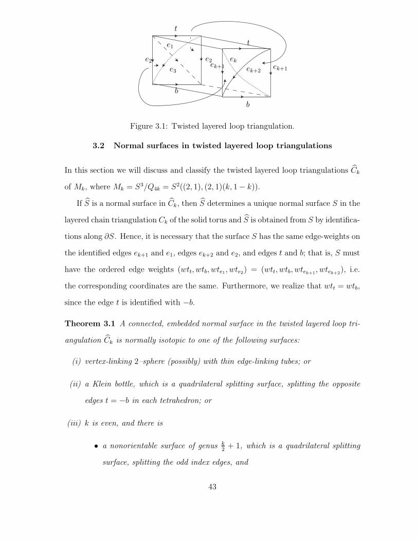
t

t

b

b

e1

e2e2

e3

ek

ek+1ek+1 ek+2

Figure 3.1: Twisted layered loop triangulation.

3.2 Normal surfaces in twisted layered loop triangulations

In this section we will discuss and classify the twisted layered loop triangulations Ck

of Mk, where Mk = S3/Q4k = S2((2, 1), (2, 1)(k, 1− k)).

If S is a normal surface in Ck, then S determines a unique normal surface S in the

layered chain triangulation Ck of the solid torus and S is obtained from S by identifica-

tions along ∂S. Hence, it is necessary that the surface S has the same edge-weights on

the identified edges ek+1 and e1, edges ek+2 and e2, and edges t and b; that is, S must

have the ordered edge weights (wtt, wtb, wte1, wte2) = (wtt, wtb, wtek+1, wtek+2

), i.e.

the corresponding coordinates are the same. Furthermore, we realize that wtt = wtb,

since the edge t is identified with −b.

Theorem 3.1 A connected, embedded normal surface in the twisted layered loop tri-

angulation Ck is normally isotopic to one of the following surfaces:

(i) vertex-linking 2–sphere (possibly) with thin edge-linking tubes; or

(ii) a Klein bottle, which is a quadrilateral splitting surface, splitting the opposite

edges t = −b in each tetrahedron; or

(iii) k is even, and there is

• a nonorientable surface of genus k2

+ 1, which is a quadrilateral splitting

surface, splitting the odd index edges, and

43

• a nonorientable surface of genus k2

+ 1, which is a quadrilateral splitting

surface, splitting the even index edges.

Remark 3.1 The double of the surface in (ii) is a thin edge-linking torus about the

edge t = −b. The doubles of the surfaces in (iii) are vertex-linking 2–spheres with

thin edge-linking tubes; in the first case of (iii), the thin edge-linking tubes are about

the odd index edges and in the second case of (iii), the thin edge-linking tubes are

about the even index edges. In all these doubles, we have quadrilateral surfaces that

fall into (i).

Proof. We only need to list the embedded normal surfaces in the layered chain trian-

gulation Ck of the solid torus as in theorem 2.2 and consider those normal surfaces

where we have ordered edge weights (wtt, wtb, wte1, wte2) = (wtt, wtb, wtek+1, wtek+2

),

and wtt = wtb.

0. No surfaces result from Vertex-linking disk. For any Vertex-linking disk,(0, 2, 1, 1);(0, 2, 1, 1)

or (2, 0, 1, 1); (2, 0, 1, 1), we can not get any normal surfaces in the twisted lay-

ered loop triangulation, since wtt 6= wtb

1. From the vertex-linking disks (possibly) with thin edge-linking tubes, (2, 2, 2, 2); (2, 2, 2, 2),

we get the vertex-linking 2–sphere (possibly) with thin edge-linking tubes. The

two vertex-linking disks are identified along their boundaries to give the single

vertex-linking 2–sphere; if there are thin edge-linking tubes, then the resulting

surface has the same thin edge-linking tubes.

2. From the vertical annulus, (0, 0, 1, 1); (0, 0, 1, 1), we have a Klein bottle, which

is a quadrilateral splitting surface, splitting the opposite edges t = −b in each

tetrahedron.

In this case the two boundaries of the vertical annulus have an orientation

reversing identification, giving a Klein bottle.

44

3. No surfaces result from the meridian disks.

For the meridian disks from 3(a) with boundary edge-weights, (1, 1, p, p+1); (1, 1, p+

k, (p + 1) + k), we have k > 0 and thus p 6= p + k.

For the meridian disks from 3(b) with boundary edge-weights, (1, 1, p+1, p); (1, 1, |(p+

1) − k|, |p − k|), we have k > 0; hence, for 0 < k ≤ p, we have 0 ≤ p − k 6= p

and for k > p, we have |(p+1)−k| < |p−k|, whereas p+1 > p. It follows that

in both cases the boundary edge-weights do not match upon identification.

4. No surfaces result from an upper edge-linking disk (possibly) with thin edge-

linking tubes, (2, 2, 2, 2); 2× (1, 1, q, q + 1) or (2, 2, 2, 2); 2× (1, 1, 1, 0), because

the boundary edge-weights do not match upon identification.

5. Similarly, no surfaces result from a lower edge-linking disk (possibly) with thin

edge-linking tubes, 2 × (1, 1, p + 1, p); (2, 2, 2, 2) or 2 × (1, 1, 0, 1); (2, 2, 2, 2).

6. If k is even we get two one-sided (nonorientable) surfaces each having genus

k2

+ 1.

(a) From the one-sided surfaces of genus c, (1, 1, 0, 1); (1, 1, 0, 1), we get a

nonorientable surface of genus k2

+ 1, S1, which is a quadrilateral splitting

surface, splitting the odd index edges.

In case 6(a) of theorem 2.2 we have a family of one-sided surface of genus c,

(1, 1, 0, 1); (1, 1, |k−2c|, (k+1)−2c), k = 2c. For a surface from this family

to give a surface in Ck, we must have the edge-weight |k − 2c| = 0, which

happens if and only if k = 2c. We noted above in Example 6(a) that this

surface is a quadrilateral splitting surface, splitting the odd index edges.

This surface has connected boundary in Ck and upon identification of its

boundary, we add another crosscap, giving a one-sided surface with genus

c + 1 = k2

+ 1 in Ck. Notice there is no other nonorientable surface exist

45

such that this surface can be compress to, therefore, it is incompressible.

(b) From the one-sided surface of genus c = k2, (1, 1, 1, 0); (1, 1, 1, 0), we get a

nonorientable surface of genus k2

+ 1, S2, which is a quadrilateral splitting

surface, splitting the even index edges.

In case 6(b) of theorem 2.2 we have a family of one-sided surface of genus

c, (1, 1, p + 1, p); (1, 1, |(k − 1) − (p + 2c)|, k − (p + 2c)), k ≥ (p + 2c). For

a surface from this family to give a surface in Ck, we must have the edge-

weight k−(p+2c) = p, which happens if and only if k = 2p+2c. However,

we also must have the edge-weight |(k−1)−(p+2c)| = p+1 for k = 2p+2c,

which happens if and only if p = 0. So, from Example 6(b) above, we

must have the one-sided surface of genus c = k2, (1, 1, 1, 0); (1, 1, 1, 0). We

noted that this surface is a quadrilateral splitting surface, splitting the

even index edges; it has connected boundary in Ck and upon identification

of its boundary, we add another crosscap, giving a one-sided surface with

genus c + 1 = k2

+ 1 in Ck, and it is incompressible.

7. Finally, we have annuli (possibly) with thin edge-linking tubes and edge-weights

in ∂Ck, 2 × (1, 1, 0, 1); 2 × (1, 1, 1, 0), or 2 × (1, 1, 0, 1); 2 × (1, 1, q, q + 1), or

2 × (1, 1, p + 1, p); 2 × (1, 1, 1, 0), or 2 × (1, 1, p + 1, p); 2× (1, 1, q, q + 1), where

p, q ≥ 0.

Obviously, we can not get a match from 2 × (1, 1, 0, 1); 2 × (1, 1, 1, 0). From

2 × (1, 1, 0, 1); 2 × (1, 1, q, q + 1), we must have q = 0 and we have the double

of the one-sided surface in 6(a),or an annulus in 7(c). From 2 × (1, 1, p +

1, p); 2 × (1, 1, 1, 0), we must have p = 0 and it is the double of the one-sided

surface in 6(b) or annulus in 7(c). In the last case where the edge-weights are

2×(1, 1, p+1, p); 2×(1, 1, q, q+1), we can never get a match, since the maximum

edge-weight is on e1 in the bottom annulus of ∂Ck but is on ek+2, not ek+1, in

46

the top annulus. These edge-weights are not match under the identification.

Note that the only surfaces we obtained from 7 are the vertex-linking 2–sphere

with thin edge-linking tubes.

This completes the proof.

Corollary 3.1 Let Mk = S3/Q4k = S2((2, 1), (2, 1), (k, 1−k)). If k is even, then Mk

has precisely three distinct (up to isotopy ) embedded, connected, one-sided, incom-

pressible surfaces; one is a Klein bottle, each of the other two have genus k2

+ 1.

Proof. It is well-known (c.f. [11, 21]) that the fundamental group of Mk is

π1Mk =< f, s1, s2, s3|[si, f ], s12f, s2

2f, s3kf, s1s2s3f

e = 1, i = 1, 2, 3 >

where the interger e is the usual Euler class representing the obstruction to ex-

tend a section given on the boundary components of regular neighborhoods of the

exceptional fibers to the complement. Here e = 1.

Therefore, the first homology group H1(Mk, Z2) is Z2 + Z2 for k is even, and is Z4

for k is odd. There is an one-sided incompressible nonorientable surface associated

with any nonzero class in H1(Mk, Z2) ∼= H1(Mk, Z2) ∼= H2(Mk, Z2) (See details in

[26]). Therefore, for k even, there are 3 nonzero class in H1(Mk, Z2) is Z2+Z2. Hence,

Mk has at least three distinct (up to isotopy), embedded, one-sided incompressible

surfaces. It follows that for any triangulation of Mk there must then be at least three

distinct, embedded, one-sided, incompressible surfaces. In particular, this is true for

the twisted layered loop triangulation Ck. Since the triangulation Ck has precisely

three one-sided normal surfaces: a Klein bottle and two surfaces each with genus

k2

+ 1, it follows that these surfaces are not isotopic and are incompressible.

47

CHAPTER 4

Layered chain pair triangulations

In this chapter we will discuss another family of triangulations, layered chain pair

triangulations, based on layered chain triangulations of the solid torus, constructed

by Ben Burton in [4].

4.1 Layered chain pair triangulations of Mr,s

The starting point for a layered chain pair triangulation is two layered chain trian-

gulations Cr and Cs of the solid torus, of length r and s, respectively. The boundary

of the solid torus in a layered chain triangulation is made up of four triangles. Two

of them make up what we are calling the top annulus and the other two make up the

bottom annulus. In the layered chain Cr we label the boundary edges τ, β, f1, f2, fr+1,

and fr+2, where the labels are analogous with those in Figure 3.24 in [4], and direct

them as in Figure 3.24 in [4]. In the layered chain Cs we label the boundary edges

t, b, e1, e2, es+1 and es+2 and direct them as in Figure 3.24 in [4]. A manifold with

triangulation is then obtained by identifying the four boundary faces of Cr with the

four boundary faces of Cs, using the following edge identifications. See Figure 4.1.

b ↔ fr+1 t ↔ −f2

e2 ↔ −τ es+1 ↔ β

e1 ↔ −f1 ↔ −es+2 ↔ fr+2.

The result is a closed 3–manifold, denoted Mr,s, and the triangulation, denoted

Cr,s, is called an (r, s) layered chain pair after [4].

48

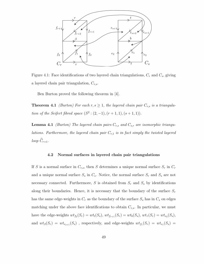
e1e2 e2

es+1

es+1es+2

t

t

b

f1 f2f2

fr+1

fr+1fr+2

τ

τ

β

CsCr

Figure 4.1: Face identifications of two layered chain triangulations, Cr and Cs, giving

a layered chain pair triangulation, Cr,s.

Ben Burton proved the following theorem in [4].

Theorem 4.1 (Burton) For each r, s ≥ 1, the layered chain pair Cr,s is a triangula-

tion of the Seifert fibred space (S2 : (2,−1), (r + 1, 1), (s + 1, 1)).

Lemma 4.1 (Burton) The layered chain pairs Cr,s and Cs,r are isomorphic triangu-

lations. Furthermore, the layered chain pair Cr,1 is in fact simply the twisted layered

loop Cr+1.

4.2 Normal surfaces in layered chain pair triangulations

If S is a normal surface in Cr,s, then S determines a unique normal surface Sr in Cr

and a unique normal surface Ss in Cs. Notice, the normal surface Sr and Ss are not

necessary connected. Furthermore, S is obtained from Sr and Ss by identifications

along their boundaries. Hence, it is necessary that the boundary of the surface Sr

has the same edge-weights in Cr as the boundary of the surface Ss has in Cs on edges

matching under the above face identifications to obtain Cr,s. In particular, we must

have the edge-weights wtf2(Sr) = wtt(Ss), wtfr+1(Sr) = wtb(Ss), wtτ (Sr) = wte2(Ss),

and wtβ(Sr) = wtes+1(Ss) , respectively, and edge-weights wtf1(Sr) = wte1(Ss) =

49

wtfr+2(Sr) = wtes+2(Ss).

In our notation, the edge-weights for the boundary of the surface Sr are given as

(wtτ , wtβ, wtf1, wtf2); (wtτ , wtβ, wtfr+1, wtfr+2); whereas, those for the surface Ss are

given as (wtt, wtb, wte1, wte2); (wtt, wtb, wtes+1, wtes+2). Hence, in order for Sr and Ss

to match to give a normal surface in Cr,s, we must have pairs of 4-tuple:

(x, y, z, u); (x, y, v, z) ↔ (u, v, z, x); (u, v, y, z), (4.1)

where the first pair (x, y, z, u); (x, y, v, z) are the parameterizations for edge-weights of

the boundary of Sr in the bottom annulus and the top annulus of Cr,respectively, and

the second pair (u, v, z, x); (u, v, y, z) are the parametrizations for the edge-weights of

the boundary of Ss in the bottom annulus and the top annulus of Cs, respectively.

From now on, we will identify the unique normal surface S obtained from Sr and Ss

by the edge-weight matching equation (x, y, z, u); (x, y, v, z) ↔ (u, v, z, x); (u, v, y, z),

determined from Sr and Ss.

Theorem 4.2 A connected, embedded, normal surface S in the triangulated chain

pair, Cr,s=Cs,r, r, s > 1 is isotopic to one of the following surfaces:

For the orientable case,

I. S is a vertex-linking s2 (possibly) with thin edge-linking tubes in all triangulation

Cr,s, r, s > 1.

It has one of the following possible edge-weight matching equations,

1. (2, 2, 2, 2); (2, 2, 2, 2) ↔ (2, 2, 2, 2); (2, 2, 2, 2)

2. 2 × (1, 1, 0, 1); 2× (1, 1, 1, 0) ↔ 2 × (1, 1, 0, 1); 2× (1, 1, 1, 0)

3. [(0, 2, 1, 1); (0, 2, 1, 1)] + [(0, 0, 1, 1); (0, 0, 1, 1)] ↔ 2 × (1, 1, 1, 0); (2, 2, 2, 2)

4. [(2, 0, 1, 1); (2, 0, 1, 1)]+[(0, 0, 1, 1); (0, 0, 1, 1)] ↔ (2, 2, 2, 2) ↔ 2×(1, 1, 0, 1)

5. 2 × (0, 0, 1, 1); 2× (0, 0, 1, 1) ↔ 2 × (1, 1, 1, 0); 2× (1, 1, 0, 1)

50

In fact, for very edge in the layered chain pair triangulation, there is a vertex-

linking S2 with a thin edge-linking tube around it. Furthermore, For any proper

compatible subsets of all edges in the layered chain pair triangulation, there is

a vertex linking S2 with thin edge-linking tubes around each edge in this subset.

II. S is an orientable normal surface, which is not a thin edge-linking tube surface.

Assume Sr in Cr has genus g′, and Ss in Cs has genus g.

1. S is a nonseparating torus in C2,5 = C5,2 with edge-weights matching equa-

tion (2, 2, 3, 1); (2, 2, 1, 3) ↔ (1, 1, 3, 2); (1, 1, 2, 3).

It is a torus fiber in the fibration of M2,5 = M5,2 over S1.

2. S is an orientable surface with genus g+2 in C2,n = Cn,2, n ≥ 7, with edge-

weights matching equation 2×(2, 2, 3, 1); 2×(2, 2, 1, 3) ↔ 2×(1, 1, 3, 2); 2×

(1, 1, 2, 3).

3. S is a nonseparating torus in C3,3 with edge-weights matching equation

(1, 1, 2, 1); (1, 1, 1, 2) ↔ (1, 1, 2, 1); (1, 1, 1, 2).

It is a torus fiber in the fibration of M3,3 over S1.

4. S is an orientable surface with genus g′ + g + 2 in C3,5 = C5,3 or Cr,s,

r, s ≥ 5, with edge-weights matching equation 2×(1, 1, 2, 1); 2×(1, 1, 1, 2) ↔

2 × (1, 1, 2, 1); 2× (1, 1, 1, 2).

For the nonorientable case,

I. r even and s odd, s = 2c + 1, c ≥ 1 (or r odd, r = 2c′ + 1, c′ ≥ 1 and s even):

1. a nonorientable incompressible surface of genus c (or c’) if r = 2, s =

2c + 1,s ≥ 7, i.e. c ≥ 3.

It has an edge-weights matching equation (2, 2, 3, 1); (2, 2, 1, 3) ↔ (1, 1, 3, 2); (1, 1, 2, 3).

The double of it is an orientable surface with genus c− 1 in the orientable

case II.2. Also, if s = 5 this surface is a nonseparating torus in C2,5.

51

2. a nonorientable, quadrilateral, splitting surface of genus c+2 (or c′ +2), if

r = 2, s = 2c+1, s ≥ 3. The edge-matching equation is (0, 0, 1, 1); (0, 0, 1, 1) ↔

(1, 1, 1, 0)(1, 1, 0, 1).

In C2,2c+1, c ≥ 2 i.e. s ≥ 5, it is a compressible surface and can be

compressed to a surface mentioned in the above case 1. Otherwise, it is

incompressible. The double of this surface is a vertex-linking S2 with c + 1

thin edge-linking tubes. It always has at least two thin edge-linking tubes

around edge τ = −e2 and β = es+1, respectively.

II. r, s both odd, r = 2c′ + 1, s = 2c + 1, c′, c ≥ 1

1. a nonorientable, incompressible, quadrilateral splitting surface of genus c+

2, with edge-weights matching equation (0, 0, 1, 1); (0, 0, 1, 1) ↔ (1, 1, 1, 0)(1, 1, 0, 1).

2. a nonorientable, incompressible, quadrilateral splitting surface of genus c′+

2, (1, 1, 1, 0)(1, 1, 0, 1) ↔ (0, 0, 1, 1); (0, 0, 1, 1).

3. a nonorientable, compressible, quadrilateral splitting surface of genus c′ +

c+2, with edge-weights matching equation (1, 1, 0, 1); (1, 1, 1, 0) ↔ (1, 1, 0, 1); (1, 1, 1, 0).

This surface can be compressed to get a surface in the following case.

4. a nonorientable, incompressible surface of genus c′ + c, except for c′ =

c = 1. It has the edge-weights matching equation (1, 1, 2, 1); (1, 1, 1, 2) ↔

(1, 1, 2, 1); (1, 1, 1, 2).

If we double this surface we will get a normal surface with genus c′+c−1 in

the orientable case II.4. When c′ = c = 1, this surface is a nonseperating

torus in C3,3 in the orientable case II.3.

Proof. As noted above, a normal surface S in Cr,s determines unique normal surfaces

Sr in Cr and Ss in Cs and is formed by identification of the boundary of Sr with

the boundary of Ss. Furthermore, in order for the boundaries of Sr and Ss to match

52

to give a normal surface in Cr,s, we must have the pairs of 4-tuples of edge-weights

match as in equation 4.1, including possible multiplicities.

For the proof, we analyze the possible matches of these 4-tuples, using the classi-

fication of normal surfaces in a layered chain triangulation of the solid torus given in

Theorem 2.2.

Notice all the families of normal surfaces in the Theorem 2.2 have edge-weight 4-

tuples satisfy the equation wtt = wtb, except for the vertex linking disk, (0, 2, 1, 1); (0, 2, 1, 1)

and (2, 0, 1, 1); (2, 0, 1, 1) in case 0. Therefore, |x − y| = 2m holds for the edge-

weights of the normal surface Sr, (x, y, z, u); (x, z, v, y), in Cr, where m is the number

of extra copies of (0, 2, 1, 1); (0, 2, 1, 1) or (2, 0, 1, 1); (2, 0, 1, 1) in case 0. If x ≥ y,

then m is where m is the number of extra copies of (0, 2, 1, 1); (0, 2, 1, 1), and vice

versa. Similarly, |u − v| = 2n holds for the the edge-weights of the boundary

of Ss, (u, v, z, x); (u, v, y, z), in Cs, where n is the the number of extra copies of

(0, 2, 1, 1); (0, 2, 1, 1) or (2, 0, 1, 1); (2, 0, 1, 1) in case 0.

Since Cr,s and Cs,r are isomorphic, we only need to consider the following 3 cases.

• if x = y and u = v,

• if x = y and u 6= v,

• if x 6= y and u 6= v.

Let’s start from the first case.

• if x = y and u = v, In order for the Sr and Ss to match to give a normal surface

in Cr,s, we must have pairs of 4-tuples:

(x, x, z, u); (x, x, u, z) ↔ (u, u, z, x); (u, u, x, z), (4.2)

we analyze the possible matches of these 4-tuples, using the classification of

normal surfaces in a layered chain triangulation of the solid torus given in

53

Theorem 2.2. Obviously that the normal surface Sr or Ss cannot be vertex

linking disk, (2, 0, 1, 1); (2, 0, 1, 1) or (0, 2, 1, 1); (0, 2, 1, 1), Since its edge-weight

does’t satisfy x = y. Hence we ignore this case. We start from Sr is from case

1 in Theorem 2.2.

Case 1. The surface Sr is the vertex-linking disks (possibly) with thin edge-

linking tubes, (2, 2, 2, 2); (2, 2, 2, 2).

The match is

(2, 2, 2, 2); (2, 2, 2, 2) ↔ (2, 2, 2, 2); (2, 2, 2, 2),

giving that Ss must also be the vertex-linking disks (possibly) with thin edge-

linking tubes. The surface S in Cr,s is the vertex-linking 2–sphere (possibly) with

thin edge-linking tubes.

Case 2.Sr is the vertical annulus, (0, 0, 1, 1); (0, 0, 1, 1).

It follows from the necessary matching of edge weights in equation 4.2 that the

edge-weights for the surface Ss must be (1, 1, 1, 0); (1, 1, 0, 1) and the match is:

(0, 0, 1, 1); (0, 0, 1, 1) ↔ (1, 1, 1, 0); (1, 1, 0, 1).

Hence, we consider the possibilities for Ss.

Possibility 2.1. Ss is from 3(b) of Theorem 2.2, a meridian disk, (1, 1, p +

1, p); (1, 1, |(p+1)− s|, |p− s|). Hence, necessarily p = 0 and s = 1 and S is the

Klein bottle in Cr+1. Since here we are assuming s > 1, we temporarily ignore

this case, and address it again in the corollary following this proof.

Possibility 2.2. Ss is from 6(b) of Theorem 2.2, a one-sided surface of genus

c ≥ 1, (1, 1, p + 1, p); (1, 1, |(s − 1) − (p + 2c)|, s − (p + 2c)), s ≥ (p + 2c). So,

necessarily p = 0 and (s − 1) − 2c = 0 giving s = 2c + 1, c ≥ 1. The surface S

in Cr,2c+1 is a nonorientable, quadrilateral, splitting surface of genus c + 2. In

54

general, this surface is is compressible, if r = 2, s = 2c + 1, s ≥ 7. Otherwise,

it is incompressible.

If r is odd, r = 2c′ +1, then we can reverse the roles of r and s and we have the

surface S in C2c′+1,s a nonorientable, quadrilateral, splitting surface of genus

c′ + 2 (See Possibility 6.2.1 below).

If r = 2c′ + 1 and s = 2c + 1 are both odd, then we have both of these

in C2c′+1,2c+1, giving distinct, nonorientable, quadrilateral, splitting surfaces of

genus c + 2 and c′ + 2.

Possibility 2.3. If we double the surface Sr, we have the match

2 × (0, 0, 1, 1); 2× (0, 0, 1, 1) ↔ 2 × (1, 1, 1, 0); 2× (1, 1, 0, 1).

.

Ss is from 7(a.1) or 7(c.1) of Theorem 2.2, an annulus with thin edge-linking

tubes, 2 × (1, 1, 1, 0); 2× (1, 1, 0, 1).

Notice if Ss is double of a meridian disk, then S is not connected which consists

of two disjoint surfaces. we ignore this case. Hence, Ss is from 7(a.1) or 7(c.1)

of Theorem 2.2, an annulus with thin edge-linking tubes, 2 × (1, 1, 1, 0); 2 ×

(1, 1, 0, 1).

In this situation, S is a vertex-linking 2–sphere that has thin edge-linking tubes.

Furthermore, S obtained from (7(a.1) is a quadrilateral vertex-linking 2–sphere

with thin edge-linking tubes which is the double of Possibility 2.2.

Case 3. Sr is from 3(b) of Theorem 2.2, a meridian disk, (1, 1, p+1, p); (1, 1, |(p+

1) − r|, |p − r|).

We have that 3(a) of Theorem 2.2 can not occur. For in this case, the edge-

weights for the boundary of the meridian disk meeting the edges in the bottom

annulus and the top annulus of Cr are (1, 1, p, p+1); (1, 1, p+r, (p+1)+r), where

55

r > 1. However, the matching from equation 4.2 would require p = p + 1 + r

i.e. r = −1, and p + 1 = p + r, which is impossible.

If we have 3(b), the edge-weights for the boundary of the meridian disk Sr is

(1, 1, p+1, p); (1, 1, |(p+1)−r|, |p−r|). Since the edge-weights for the boundary

of the meridian disk meeting the edges in the bottom annulus is (1, 1, p + 1, p),

it follows from equation 4.2 that the match is

(1, 1, p + 1, p); (1, 1, p, p + 1) ↔ (p, p, p + 1, 1); (p, p, 1, p + 1),

By comparing the coordinates of the edge-weights in the above equation, we

have r = 2p + 1. we also notice Sr is a meridian disk from 3(b), (1, 1, p +

1, p); (1, 1, p, p + 1), p ≥ 0.

Now, we consider the possibilities for the surface Ss. Its edge-weights must be

(p, p, p + 1, 1); (p, p, 1, p + 1).

notice the edge-weights for the boundary of Ss meeting the edges in the bottom

annulus is

(p, p, p + 1, 1) =

(1, 1, 2, 1) + (p − 1) × (1, 1, 1, 0), p ≥ 2

(1, 1, 2, 1), p = 1

(0, 0, 1, 1), p = 0

(4.3)

Let’s consider the case p ≥ 2, the edge-weights for the boundary of Ss meeting

the edges in the bottom annulus is

(p, p, p + 1, 1) = (1, 1, 2, 1) + (p − 1) × (1, 1, 1, 0)

push−→ (1, 1, 1, 0) + (p − 1) × (1, 1, 0, 1)

push−→ (1, 1, 0, 1) + (p − 1) × (1, 1, 1, 2)

push−→ (1, 1, 1, 2) + (p − 1) × (1, 1, 2, 3)

push−→ · · ·

push−→ (1, 1, p′, p′ + 1) + (p − 1) × (1, 1, p′ + 1, p′ + 2), p′ ≥ 0

56

Hence, the edge-weights for the boundary of Ss meeting the edges in the top

annulus with bottom edge-weights (p,p,p+1,1)can only possible be

(1, 1, 1, 0) + (p − 1) × (1, 1, 0, 1), or

(1, 1, p′, p′ + 1) + (p − 1) × (1, 1, p′ + 1, p′ + 2), p′ ≥ 0

While, according to the match (1, 1, p+1, p); (1, 1, p, p+1) ↔ (p, p, p+1, 1); (p, p, 1, p+

1), the edge-weights for the boundary of Ss meeting the edges in the top annulus

need to be

(p, p, 1, p + 1) =

(1, 1, 1, 2) + (p − 1) × (1, 1, 0, 1), p ≥ 2

(1, 1, 1, 2), p = 1

(0, 0, 1, 1), p = 0

(4.4)

Notice, for p ≥ 2 case, if (1, 1, 1, 2) + (p − 1) × (1, 1, 0, 1) = (1, 1, 1, 0) + (p −

1) × (1, 1, 0, 1), or (1, 1, p′, p′ + 1) + (p − 1) × (1, 1, p′ + 1, p′ + 2), p′ ≥ 0, we

get p can only be 2, and the edge-weights of Ss are (2, 2, 3, 1); (2, 2, 1, 3) i.e.

(1, 1, 2, 1) + (1, 1, 1, 0); (1, 1, 0, 1) + (1, 1, 1, 2)

Therefore, if the surfaces Sr with Ss together satisfying

(1, 1, p + 1, p); (1, 1, p, p + 1) ↔ (p, p, p + 1, 1); (p, p, 1, p + 1);

Therefore, p = 0, p = 1, or p = 2.

Possibility 3.1. If p = 0, the match is (0, 0, 1, 1); (0, 0, 1, 1) ↔ (1, 1, 1, 0); (1, 1, 0, 1).

Notice that no meridian disk is of the boundary edge-weights (0, 0, 1, 1), (0, 0, 1, 1).

Hence this case is impossible.

Possibility 3.2. If p = 1, then r = 3 and the match is (1, 1, 2, 1); (1, 1, 1, 2) ↔

(1, 1, 2, 1); (1, 1, 1, 2). For this case, there are two possibilities for Ss.

57

Possibility 3.2.1. Ss is from 3(b) of Theorem 2.2, a meridian disk, (1, 1, 2, 1); (1, 1, s−

2, s − 1), s > 1.

From this we have s − 2 = 1, s = 3; S3 is a meridian disk in Cs = C3 with

boundary edge-weights (1, 1, 2, 1); (1, 1, 1, 2) and joining it with the meridian

disk S3 in Cr = C3 we have the triangulation is C3,3 and S is the torus fiber in

the fibration of M3,3 over S1.

Possibility 3.2.2. Ss is from 6(b) of Theorem 2.2, a one-sided surface of genus

c, (1, 1, 2, 1); (1, 1, |s− 2 − 2c|, s − 1 − 2c), s ≥ 2c + 1.

From this we have s − 1 − 2c = 2 i.e. s = 2c + 3, c ≥ 1. When we calculate

the Euler characteristics of the normal surface S in this case, we have a nonori-

entable surface of genus c+2; thus in C2c+1 the nonorientable genus is c+1. In

C3,2c+1 we have a nonorientable, incompressible surface of genus 1 + c. (Note

this is related to Possibility 6.2.2 below and for 3 = 2c′ + 1, c′ = 1 and we have

genus c′ + c = 1 + c as in that possibility.)

Possibility 3.2.3. Ss is from 7 of Theorem 2.2, an annulus with thin edge-linking

tubes, 2 × (1, 1, 2, 1); 2× (1, 1, 1, 2).

This is case that we double the edge-weights of Sr and Ss, we have the match

2 × (1, 1, 2, 1); 2 × (1, 1, 1, 2) ↔ 2 × (1, 1, 2, 1); 2 × (1, 1, 1, 2). Thus in Cr = C3

we have two copies of a meridian disk, (1, 1, 2, 1); (1, 1, 1, 2) and in Cs we have

2 possibilities. One is two copies of meridian disk, 2 × (1, 2, 1); 2× (1, 1, 2). we

will get two copies of S in C3,3. We ignore this case. The other one is from 7

of Theorem 2.2. Furthermore, it is from 7(b.2) or 7(c.4). Both of them give us

the vertex-linking 2–sphere with thin edge-linking tubes. Notice the one from

7(b.2) is the double of the one-sided surface in Possibility 3.2.2.

Possibility 3.3. If p = 2, then r = 5 and the match is (1, 1, 3, 2); (1, 1, 2, 3) ↔

(2, 2, 3, 1); (2, 2, 1, 3). For this case, Ss can only be two disjoint meridian disks

58

with edge-weight (1, 1, 2, 1) + (1, 1, 1, 0); (1, 1, 0, 1) + (1, 1, 1, 2).

Notice (1, 1, 2, 1)+(1, 1, 1, 0)push−→ (1, 1, 1, 0)+(1, 1, 0, 1)

push−→ (1, 1, 0, 1)+(1, 1, 1, 2)

Obviously, Ss can only be two disjoint meridian disks. In C5,2, we calculate the

Euler characteristics of the normal surface S, we get S is a torus.

If we double the edge-weights of S, we get two disjoint surfaces, so we ignore

this case.

Now we need to consider the case that we have any combination of meridian

disks, n1m1 + n2m2 + ... + nkmk, where ni ∈ {1, 2, ...}, and mi is any meridian

disk from case 3.

Notice,

– If Cr consists of n copies of a meridian disks, by the above argument, then

we may have n copies of disjoint surfaces S.

– If Cr consists of different copies of different type of meridian disks, some of

which are from 3(a), others are from 3(b), there are two different quadrilat-

eral normal disks in the same tetrahedron. This contradicts to the quadri-

lateral condition that it can not contain more than one type of quadrilateral

normal disk in one tetrahedron. Hence all of the meridian disks, summands

of Cr, are either all from 3(a), or all from 3(b).

– If Cr is only from the combination of meridian disks from 3(a), n1m1 +

n2m2 + ... + nkmk, then the bottom edge-weights of it is n1(1, 1, p1, p1 +

1) + n2(1, 1, p2, p2 + 1) + ... + nk(1, 1, pk, pk + 1) = (t, t, u, t + u), where t,

u are positive intergers. However,the matching from equation 4.2 would

require the top edge-weights of it is (t, t, t+u, u), which is impossible since

the weights (t, t, u, t + u) can only be (t, t, u + k, t + u + k) obtained by

push.

59

Hence Cr can only be any combination of meridian disks, n1m1 + n2m2 + ... +

nkmk, where ni ∈ {1, 2, ...}, where mi is any meridian disk from 3(b) with

bottom edge-weights (t, t, t + v, v). Therefore, Cr is the disconnected surface

with edge-weights (t, t, t + v, v); (t, t, v, t + v) Now consider Cr’s the bottom

edge-weights (t, t, t + v, v). It’s not difficult to show that:

(t, t, t+v, v) =

v(1, 1, 2, 1) + (t − v)(1, 1, 1, 0), t > v

t(1, 1, 2, 1), t = v

r(1, 1, n + 2, n + 1) + (t − r)(1, 1, n + 1, n), t < v, v = nt + r

(4.5)

If the bottom edge-weights of the surface is (t, t, v, t + v), by same argument as

above we get

(t, t, v, t + v) =

v(1, 1, 1, 2) + (t − v)(1, 1, 0, 1), t > v

t(1, 1, 1, 2), t = v

r(1, 1, n, n + 2) + (t − r)(1, 1, n, n + 1), t < v, v = nt + r

(4.6)

For Cr, the surface of any combination of meridian disks, where all meridian

disks are from 3(b) with edge-weights (t, t, t + v, v); (t, t, v, t + v), there are 3

possibilities by considering its bottom edge-weights:

– The first case t > v.

Possibility 3.4. Cr is two disjoint meridian disks (1, 1, 2, 1); (1, 1, 0, 1) and

(1, 1, 1, 0); (1, 1, 1, 2), where r = 2

For t > v, Cr the surface of any combination of meridian disks, where all

meridian disks are from 3(b) with edge-weights (t, t, t + v, v); (t, t, v, t + v)

with t > v.

(t, t, t + v, v) =v(1, 1, 2, 1) + (t − v)(1, 1, 1, 0)

push−→ v(1, 1, 1, 0) + (t − v)(1, 1, 0, 1)

60

push−→ v(1, 1, 0, 1) + (t − v)(1, 1, 1, 2)

push−→ · · ·

push−→ v(1, 1, p, p + 1) + (t − v)(1, 1, p + 1, p + 2), p ≥ 0.

From the above, we notice that in order to have the top edge-weights

(t, t, v, t + v), we need to require v = t − v, i.e. t = 2v. Hence, Cr with

edge-weights

(2v, 2v, 3v, v); (2v, 2v, v, 3v) = v[(2, 2, 3, 1); (2, 2, 1, 3)]

= v[(1, 1, 2, 1) + (1, 1, 1, 0); (1, 1, 0, 1) + (1, 1, 1, 2)].

. This is v copies of the sum of two meridian disks (1, 1, 2, 1); (1, 1, 0, 1)

and (1, 1, 1, 0); (1, 1, 1, 2).

Consider one copy of the sum of two meridian disks (1, 1, 2, 1); (1, 1, 0, 1)

and (1, 1, 1, 0); (1, 1, 1, 2). Look at the matching equation 4.2. We have the

match:

(2, 2, 3, 1); (2, 2, 1, 3) ↔ (1, 1, 3, 2); (1, 1, 2, 3), i.e.

(1, 1, 2, 1) + (1, 1, 1, 0); (1, 1, 0, 1) + (1, 1, 1, 2) ↔ (1, 1, 3, 2); (1, 1, 2, 3).

There are two possibilities for cs with edge-weights (1, 1, 3, 2); (1, 1, 2, 3).

Possibility 3.4.1. Cr is two disjoint meridian disks (1, 1, 2, 1); (1, 1, 0, 1) and

(1, 1, 1, 0); (1, 1, 1, 2), where r = 2. Cs is a meridian disk, (1, 1, 3, 2); (1, 1, 2, 3),

with s = 5. This gives us that S is a torus.

Possibility 3.4.2. Cr is two disjoint meridian disks (1, 1, 2, 1); (1, 1, 0, 1) and

(1, 1, 1, 0); (1, 1, 1, 2), where r = 2. Cs is a a one-sided nonorientable surface

of genus c from 6(b), (1, 1, 3, 2); (1, 1, 2, 3). Since p = 2, then r = 2c + 5.

so S2c+5 is a one-sided nonorientable surface of genus c, c ≥ 1. This

is equivalently to say S2c+1 is a one-sided nonorientable surface of genus

61

c − 2, c ≥ 3. In this case s ≥ 7. S is an incompressible non-orientable

surface in C2,2c+1 with genus c − 2 + 2 = c, where c ≥ 7, i.e s ≥ 7.

Now consider two copies of the sum of two meridian disks (1, 1, 2, 1); (1, 1, 0, 1)

and (1, 1, 1, 0); (1, 1, 1, 2). Look at the matching equation 4.2. We have the

match:

2 × (2, 2, 3, 1); 2× (2, 2, 1, 3) ↔ 2 × (1, 1, 3, 2); (1, 1, 2, 3), i.e.

2 × [(1, 1, 2, 1) + (1, 1, 1, 0)]; 2× [(1, 1, 0, 1) + (1, 1, 1, 2)]

↔ 2 × (1, 1, 3, 2); 2× (1, 1, 2, 3).

Possibility 3.4.3. Cr is two copies of two disjoint meridian disks (1, 1, 2, 1); (1, 1, 0, 1)

and (1, 1, 1, 0); (1, 1, 1, 2), where r = 2 and cs is from 7(b.2) or 7(c.4) of The-

orem 2.2. Any of the resulting surfaces is a vertex-linking 2–sphere with

thin edge-linking tubes. The one with Ss from 7(b.2) is the double of the

one-sided surface from Possibility 3.4.2..

Notice, if v ≥ 3, we will get disjoint surface S. We ignore this case.

– The second case t = v. We have Cr is any combination of meridian

disks, where all meridian disks are from 3(b) with edge-weights (t, t, t +

v, v); (t, t, v, t + v), s.t. t = v. Therefore, Cr’s t copies of meridian disks

(1, 1, 2, 1); (1, 1, 1, 2). Which is the same case as Possibility 3.2.

– The third case t < v. We have Cr is any combination of meridian disks,

where all meridian disks are from 3(b) with edge-weights (t, t, t+v, v); (t, t, v, t+

v), s.t. t < v. Then Cr is some combination of meridian disks r(1, 1, n +

2, n + 1) + (t− r)(1, 1, n + 1, n); r(1, 1, n+ 1, n + 2) + (t− r)(1, 1, n, n + 1),

where v = nt + r. Let’s consider the possible top edge-weights of the sur-

faces with bottom edge-weights (1, 1, n+2, n+1)+(t−r)(1, 1, n+1, n).By

the same argument as above, we have r = t − r, i.e. t = 2r.

62

If r = 0, Cr is t copies of meridian surface, (1, 1, n + 1, n); (1, 1, n, n + 1).

We discuss this case before. If r > 0, Cr is the sum of r copies of 2 meridian

surfaces, (1, 1, n+2, n+1)+(1, 1, n+1, n); (1, 1, n+1, n+2)+(1, 1, n, n+1).

Look at the matching equation 4.2. We have the match:

(1, 1, n + 2, n + 1) + (1, 1, n + 1, n); (1, 1, n + 1, n + 2) + (1, 1, n, n + 1)

↔ (1, 1, n+1, n+2)+(1, 1, n, n+1); (1, 1, n+2, n+1)+(1, 1, n+1, n+2)

Notice if this is the case, then Cs is of edge-weights (1, 1, n + 1, n + 2) +

(1, 1, n, n + 1); (1, 1, n + 2, n + 1) + (1, 1, n + 1, n + 2), which is impossible.

Case 4. Sr is from 4 of Theorem 2.2, an upper edge-linking disk, (2, 2, 2, 2); 2×

(1, 1, q, q + 1). From the matching in equation 4.2, we would necessarily have

2 = 2q and 2 = 2 + 2q, which is impossible.

Case 5. Sr is from 5 of Theorem 2.2, a lower edge-linking disk, 2 × (1, 1, p +

1, p); (2, 2, 2, 2). Similar to Case 4, this situation is impossible.

Case 6. Sr is from 6 of Theorem 2.2, either 6(a) or 6(b).

Possibility 6.1. Sr is from 6(a), a one-sided surface of genus c′, (1, 1, 0, 1); (1, 1, |r−

2c′|, (r + 1)− 2c′), r ≥ 2c′ − 1. In this case, By matching equation 4.2, we have

the match: (1, 1, 0, 1); (1, 1, 1, 0) ↔ (1, 1, 0, 1); (1, 1, 1, 0). Hence, the boundary

edge-weights for the surface Sr are (1, 1, 0, 1); (1, 1, 1, 0), hence r + 1 − 2c′ = 0,

i.e. r = 2c′ − 1.

The only possibility for the surface Ss in this case is a one-sided surface of genus

c from 6(a) with s = 2c− 1. Now, changing the index to match that above, we

have for r = 2c′+1 with c′ ≥ 0 and s = 2c+1 with c ≥ 0, nonorientable surfaces,

Sr and Ss, of genus c′+1 and c+1, respectively. Considering how these surfaces

are attached along their boundaries, we have in C2c+1,2c′+1 a nonorientable,

63

compressible, quadrilateral splitting surface of genus c′ + c + 2. Notice that this

surface compresses about the valence 4 edge e1 ↔ −f1 ↔ −es+2 ↔ fr+2.

Possibility 6.2. Sr is from 6(b), a one-sided surface of genus c′, (1, 1, p +

1, p); (1, 1, |(r − 1) − (p + 2c′)|, r − (p + 2c′), r ≥ p + 2c′. Again, we look at

the matching equation 4.2. We have

(1, 1, p + 1, p); (1, 1, p, p + 1) ↔ (p, p, p + 1, 1); (p, p, 1, p + 1)

Hence, p+1 = r− (p+2c′) and therefore, r = 2p+2c′ +1, c′ ≥ 1. By the same

argument in case 3, we get p = 0, p = 1, or p = 2.

Possibility 6.2.1. Suppose p = 0, we have Sr is a one-sided surface of genus c′,

r = 2c′ + 1.

Look at the matching equation 4.2. We have the match:

(1, 1, 1, 0); (1, 1, 0, 1) ↔ (0, 0, 1, 1); (0, 0, 1, 1).

This is the reversal of the roles of r and s from Possibility 2.2 above and we

have Sr is a one-sided surface of genus c′, r = 2c′ + 1, and Ss is the vertical

annulus. Hence, The surface S in C2c′+1,s is a nonorientable, quadrilateral,

splitting surface of genus c′ + 2. In general, this surface is compressible, if

r = 2c′ + 1, s = 2, r ≥ 7. Otherwise, it is incompressible.

Possibility 6.2.2. Suppose p = 1. we have Sr is a one-sided surface of genus c′,

r = 2c′ + 3

we look at the matching equation 4.2. We have the match:

(1, 1, 2, 1); (1, 1, 1, 2) ↔ (1, 1, 2, 1); (1, 1, 1, 2).

Hence, r = 2c′ + 3 and s is odd, say s = 2c + 3. If c = 0 and s = 3, then we

have Ss = S3 is a meridian disk and we have the reverse roles of r and s from

Possibility 3.2 above.

64

If c 6= 0 6= c′, then upon identification, we have a nonorientable, incompressible

surface of genus c′ + c + 2. Hence, for r = 2c′ + 1, s = 2c + 1, the nonorientable

genera of Sr and Ss are c′−1 and c−1, respectively. Combining these results with

those of Case 3 above which handles these surfaces when either r = 3 or s = 3,

we have in C2c′+1,2c+1, except for c′ = 1 = c, a nonorientable, incompressible

surface of genus c′ + c; for c′ = 1 = c and in C3,3, this surface is the torus fiber

in the fibration of M3,3 over S1. In all cases, these surfaces are compressions of

a surface in Possibility 6.2.1.

Notice that for either r = 3 or s = 3, the surfaces found in Case 3 are special

cases of this family of surfaces where S3 in Cr, r = 3, is a meridian disk rather

than a one-sided surface. The genus of the surface S in C2c′+1,2c+1 is c′ + c and

agrees with the special cases c′ = 1, c > 1 or c = 1, c′ > 1.

Possibility 6.3. Suppose p = 2. we have Sr is a one-sided surface of genus c′,

and r = 2c′ + 5, where c′ ≥ 1. Hence r ≥ 7

Look at the matching equation 4.2. We have the match:

(1, 1, 3, 2); (1, 1, 2, 3) ↔ (2, 2, 3, 1); (2, 2, 1, 3), i.e.

(1, 1, 3, 2); (1, 1, 2, 3) ↔ [(1, 1, 2, 1) + (1, 1, 1, 0)]; [(1, 1, 0, 1) + (1, 1, 1, 2)]

Since p = 2, then r = 2c′ + 5. so S2c′+5 is a one-sided nonorientable surface of

genus c′, c′ ≥ 1. This is equivalently to say S2c′+1 is a one-sided nonorientable

surface of genus c′ − 2, c′ ≥ 3. In this case r ≥ 7. Ss can only be two

disjointed meridian disks (1, 1, 2, 1); (1, 1, 1, 0) and (1, 1, 1, 0); (1, 1, 1, 2). By the

same argument as Possibility 3.3., s = 2. Therefore, S is a non-orientable

surface in C2c′ + 1, 2 with genus c′ − 2 + 2 = c′. This is an incompressible

surface, a compression of Possibility 6.2.1., when c′ ≥ 3 i.e. r ≥ 7.

Case 7. Sr is from 7 of Theorem 2.2, an annulus possible with thin edge-

linking tubes. We notice that the edge-weights for the boundary of Sr meeting

65

the edges in the bottom annulus is either 2 × (1, 1, 0, 1) or 2 × (1, 1, p + 1, p).

Possibility 7.1. Sr is an annulus (possibly) with thin edge-linking tubes with

bottom edge-weights 2 × (1, 1, 0, 1).we get the matching of the boundary edge-

weights for Sr with those of Ss as

2 × (1, 1, 0, 1); 2× (1, 1, 1, 0) ↔ 2 × (1, 1, 0, 1); 2× (1, 1, 1, 0).

The only possibilities for Sr are from 7(a.1) and 7(c.1) of Theorem 2.2. The

possibility for Ss is from 3, 7(a.1) or 7(c.1). In any case, the resulting surface

is a vertex-linking 2–sphere with thin edge-linking tubes, and the one with

Sr and Ss both from 7(a.1) is the double of the one-sided surface from 6.1

above,the resulting surfaces is a quadrilateral vertex-linking 2–sphere with thin

edge-linking tubes.

Possibility 7.2. Sr is an annulus (possibly) with thin edge-linking tubes with

bottom edge-weights 2×(1, 1, p+1, p), then it is from 7(b.2) or 7(c.4) of Theorem

2.2. Since the bottom edge-weight is 2× (1, 1, p + 1, p), we get the matching of

the boundray edge-weights for Sr with those of Ss as

2 × (1, 1, p + 1, p); 2 × (1, 1, p, p + 1) ↔ 2 × (p, p, p + 1, 1); 2 × (p, p, 1, p + 1).

Hence p = 0, p = 1 or p = 2.

Possibility 7.2.1. Suppose p = 0. Sr is from 7(b.2) or 7(c.4) of Theorem 2.2, an

annulus possible with thin edge-linking tubes, 2× (1, 1, 1, 0); 2× (1, 1, 0, 1). By

the matching equation 4.2, we have the match:

2 × (1, 1, 1, 0); 2× (1, 1, 0, 1) ↔ 2 × (0, 0, 1, 1); 2× (0, 0, 1, 1).

Hence, Ss is two copies of the vertical annulus. The resulting surfaces is a

vertex-linking 2–sphere with thin edge-linking tubes. The one with Sr from

7(b.2) is the double of the one-sided surface from Possibility 6.2.1 above and we

66

have Sr is the double of a one-sided surface of genus c′, r = 2c′ + 1, This is the

reversal of the roles of r and s in Possibility 2.3 above.

Possibility 7.2.2. Suppose p = 1. Sr is from 7(b.2) or 7(c.4) of Theorem 2.2, an

annulus possible with thin edge-linking tubes, 2× (1, 1, 2, 1); 2× (1, 1, 1, 2). By

the matching equation 4.2, we have the match:

2 × (1, 1, 2, 1); 2× (1, 1, 1, 2) ↔ 2 × (1, 1, 2, 1); 2× (1, 1, 1, 2).

Hence, Ss is also from two copies of 3, 7(b.2) or 7(c.4). Any of the resulting

surfaces is a vertex-linking 2–sphere with thin edge-linking tubes. The one

with Sr and Ss both from 7(b.2) is the double of the one-sided surface from

Possibility 6.2.2 above and we have Sr is the double of a one-sided surface of

genus c′, r = 2c′ + 1, This is the reversal of the roles of r and s in Possibility

6.2.2. above.

Possibility 7.2.3 Suppose p = 2. Sr is from 7(b.2) or 7(c.4) of Theorem 2.2, an

annulus possible with thin edge-linking tubes, 2× (1, 1, 3, 2); 2× (1, 1, 2, 3). By

the matching equation 4.2, we have the match:

2 × (1, 1, 3, 2); 2× (1, 1, 2, 3) ↔ 2 × (2, 2, 3, 1); 2× (2, 2, 1, 3),

i.e.(1, 1, 3, 2); (1, 1, 2, 3) ↔ [(1, 1, 2, 1) + (1, 1, 1, 0)]; [(1, 1, 0, 1) + (1, 1, 1, 2)]

We have Ss is the two copies of two disjoint meridian disks (1,1,2,1);(1,1,1,0)

and (1,1,1,0);(1,1,1,2). Notice s = 2. Any of the resulting surfaces is a vertex-

linking 2–sphere with thin edge-linking tubes. The one with Sr from 7(b.2) is

the double of the one-sided surface from Possibility 6.3.

2. if x = y and u 6= v,

We know Sr can be any family of normal surfaces including the vertex-linking

pair except copies of only one type of vertex-linking disk (2, 0, 1, 1); (2, 0, 1, 1) or

67

(0, 2, 1, 1); (0, 2, 1, 1). The possibilities of Sr is the same as the discussion in the above

case. However, u 6= v, it means that Ss can only consist of copies of only one type

vertex-linking disks (2, 0, 1, 1); (2, 0, 1, 1) or (0, 2, 1, 1); (0, 2, 1, 1) or the combination

of them with other normal surfaces. It is also easy to see that If we have more than

one copy of vertex-linking disk in the above cases, we can never have a connected

surface S in Cr,s obtained by identifying the boundaries of the Sr and Ss.

we start to analyze the possible matches of these 4-tuples, using the classification of

normal surfaces in a layered chain triangulation of the solid torus given in Theorem

2.2. we must have the pairs of 4-tuples of edge-weights match as in equation 4.1,

including possible multiplicities.

case 1. The surface Sr is the vertex-linking disks (possibly) with thin edge-linking

tubes, (2, 2, 2, 2); (2, 2, 2, 2). The match is

(2, 2, 2, 2); (2, 2, 2, 2) ↔ (2, 2, 2, 2); (2, 2, 2, 2),

giving that Ss must also be the vertex-linking disks (possibly) with thin edge-linking

tubes. Hence U = V = 2. This contradicts the fact that u 6= v.

Case 2. Sr is the vertical annulus, (0, 0, 1, 1); (0, 0, 1, 1) It follows from the nec-

essary matching of edge weights in equation 4.1 that the edge-weights for the surface

Ss must be (1, 1, 1, 0); (1, 1, 0, 1) and the match is:

(0, 0, 1, 1); (0, 0, 1, 1) ↔ (1, 1, 1, 0); (1, 1, 0, 1).

Hence, Hence U = V = 1. This contradicts the fact that u 6= v.

Case 3. Sr is a meridian disk from 3(a) or 3(b) of Theorem 2.2.

Possibility 3.1 Sr is a meridian disk from 3(a),(1, 1, p, p+1); (1, 1, p+ r, p+1+ r).

It follows from the necessary matching of edge weights in equation 4.1 that z = p and

z = p + 1 + r, which is impossible, since r 6= −1.

Possibility 3.2 Sr is a meridian disk from 3(b), (1, 1, p+1, p); (1, 1, |(p+1)−r|, |p−

r|). It follows from the necessary matching of edge weights in equation 4.1 that u = p,

68

v = |(p + 1) − r|,z = p + 1 and z = |p − r|.

From z = p + 1 = |p − r|, we get

p + 1 =

p − r, p > r

0, p = r

r − p, p < r

(4.7)

. Obviously, if p > r, then r = −1. If p = r, p = −1. They are all impossible. If

p < r, we get p+1 = r−p, hence r = 2p+1, where p is a nonnegative integer. Hence

we have u = p, v = |(p + 1) − r| = r − (p + 1) = p. This contradicts the fact u 6= v.

Case 4. Sr is from 4 of Theorem 2.2, an upper edge-linking disk, (2, 2, 2, 2); 2 ×

(1, 1, 1, 0) or (2, 2, 2, 2); 2× (1, 1, q, q + 1).

Possibility 4.1 If Sr is from 4 of Theorem 2.2, an upper edge-linking disk, (2, 2, 2, 2); 2×

(1, 1, 1, 0). We would necessarily have u = v = 2, from the matching in equation 4.1.

This is impossible.

Possibility 4.2 If Sr is from 4 of Theorem 2.2, an upper edge-linking disk, (2, 2, 2, 2); 2×

(1, 1, q, q + 1).

It follows from the necessary matching of edge weights in equation 4.1 that u = 2,

v = 2q, z = 2 and z = 2(q + 1). From z = 2 = 2(q + 1), we have q = 0, hence v = 0.

Then the edge-weight of the boundary of normal surface Ss is (2, 0, 2, 2); (2, 0, 2, 2),

which is the sum of edge-weights (2, 0, 1, 1); (2, 0, 1, 1) and (0, 0, 1, 1); (0, 0, 1, 1). Hence

the matching equation is

(2, 2, 2, 2); 2× (1, 1, 0, 1) ↔ (2, 0, 2, 2); (2, 0, 2, 2),

i.e.

(2, 2, 2, 2); 2× (1, 1, 0, 1) ↔ [(2, 0, 1, 1); (2, 0, 1, 1) + (0, 0, 1, 1); (0, 0, 1, 1)]

This gives us the vertex-linking S2 with a thin edge-linking tube around the edge

fr+1 = b in Cr,s and possibly with other thin edge-linking tubes.

69

Since we can reverse the role of r and s, so we can get a vertex-linking S2 with a

thin edge-linking tube around the edge es+1 = β in Cr,s and possibly with other thin

edge-linking tubes, with the matching equation

[(2, 0, 1, 1); (2, 0, 1, 1) + (0, 0, 1, 1); (0, 0, 1, 1)] ↔ (2, 2, 2, 2); 2× (1, 1, 0, 1)

Case 5. Sr is from 5 of Theorem 2.2, a lower edge-linking disk, 2×(1, 1, 0, 1); (2, 2, 2, 2)

or 2 × (1, 1, p + 1, p); (2, 2, 2, 2).

Possibility 5.1 If Sr is from 5 of Theorem 2.2, an lower edge-linking disk, 2 ×

(1, 1, 0, 1); (2, 2, 2, 2). We would necessarily have u = v = 2, from the matching in

equation 4.1. This is impossible.

Possibility 5.2 If Sr is from 5 of Theorem 2.2, an Lower edge-linking disk, 2 ×

(1, 1, p + 1, p); (2, 2, 2, 2).

It follows from the necessary matching of edge weights in equation 4.1 that u = p,

v = 2, z = 2 and z = 2(p + 1).From z = 2 = 2(p + 1), we have p = 0, hence u = 0.

Then the edge-weight of the boundary of normal surface Ss is (0, 2, 2, 2); (0, 2, 2, 2),

which is the sum of edge-weights (0, 2, 1, 1); (0, 2, 1, 1) and (0, 0, 1, 1); (0, 0, 1, 1). Hence

the matching equation is

2 × (1, 1, 1, 0); (2, 2, 2, 2) ↔ (0, 2, 2, 2); (0, 2, 2, 2),

i.e.

2 × (1, 1, 1, 0); (2, 2, 2, 2) ↔ [(0, 2, 1, 1); (0, 2, 1, 1) + (0, 0, 1, 1); (0, 0, 1, 1)]

This gives us the vertex-linking S2 with a thin edge-linking tube around the edge

f2 = −t in Cr,s and possibly with other thin edge-linking tubes.

Since we can reverse the role of r and s, so we can get a vertex-linking S2 with a

thin edge-linking tube around the edge e2 = −τ in Cr,s and possibly with other thin

edge-linking tubes, with the matching equation

[(0, 2, 1, 1); (0, 2, 1, 1) + (0, 0, 1, 1); (0, 0, 1, 1)] ↔ 2 × (1, 1, 1, 0); (2, 2, 2, 2)

70

Case 6. Sr is from 6 of Theorem 2.2, either 6(a) or 6(b).

Possibility 6.1. Sr is from 6(a), a one-sided surface of genus c′, (1, 1, 0, 1); (1, 1, |r−

2c′|, (r + 1) − 2c′), r ≥ 2c′ − 1. In this case, By matching equation 4.1, we get

z = 0 = k +2c−1, which meansk = 2c−1, U = 1 and v = |r−2c′|. Since k = 2c−1,

so v = |r − 2c′| = |2c − 1 − 2c| = 1. Hence,u = v = 1, which is a contradiction.

Possibility 6.2. Sr is from 6(b), a one-sided surface of genus c′, (1, 1, p+1, p); (1, 1, |(r−

1) − (p + 2c′)|, r − (p + 2c′), r ≥ p + 2c′. Again, we look at the matching equation

4.1. We get u = p,v = |r − 1) − (p + 2c′)| and z = p + 1 = r − (p + 2c′). The last

relation gives us r = 2p + 1 + 2c′. Hence v = |2p + 1 + 2c′ − 1 − p − 2c′| = 0.Hence

z = r − (p + 2c′) = 1 = p + 1 ,which means p = 0. Therefore, u = p = 0 = v, which

is a contradiction.

Case 7. Sr is from 7 of Theorem 2.2, an annulus possible with thin edge-linking

tubes with edge weight 2× (1, 1, 0, 1); 2× (1, 1, 1, 0), 2× (1, 1, 0, 1); 2× (1, 1, q, q + 1),

2× (1, 1, 0, 1); 2× (1, 1, 1, 0), 2× (1, 1, p+1, p); 2× (1, 1, 1, 0) or 2× (1, 1, p+1, p); 2×

(1, 1, q, q + 1).

Possibility 7.1. Sr is an annulus (possibly) with thin edge-linkin tubes with edge-

weights 2 × (1, 1, 0, 1); 2 × (1, 1, 1, 0). Obviously it implies u = v = 2, which is a

contradiction.

Possibility 7.2. Sr is an annulus (possibly) with thinedge-linking tubes with edge-

weights 2 × (1, 1, 0, 1); 2 × (1, 1, q, q + 1). It implies that z = 0 = 2(q + 1).Hence q is

negative, which is impossible.

Possibility 7.3. Sr is an annulus (possibly) with thin edge-linking tubes with edge-

weights 2× (1, 1, p + 1, p); 2× (1, 1, 1, 0). This implies thatz = 2(p + 1) = 0. Hence p

is negative, which is impossible.

Possibility 7.4. Sr is an annulus (possibly) with thin edge-linking tubes with edge-

weights 2 × (1, 1, p + 1, p); 2 × (1, 1, q, q + 1). This implies thatu = 2p,v = 2q,z =

2(p + 1) = 2(q + 1). From the last relation, we get p = q. Hence u = v, which is a

71

contradiction.

3. if x 6= y and u 6= v.

In this case, Sr can only consist of copies of only one type vertex-linking disks

(2, 0, 1, 1); (2, 0, 1, 1) or (0, 2, 1, 1); (0, 2, 1, 1) or the combination of them with other

normal surfaces, which include vertex-linking disk pairs.

Case 1. If Sr is a vertex-linking disk (2, 0, 1, 1); (2, 0, 1, 1) or (0, 2, 1, 1); (0, 2, 1, 1).

Possibility 1.1. If Sr is a vertex-linking disk (2, 0, 1, 1); (2, 0, 1, 1).By the matching

equation, we get

(2, 0, 1, 1); (2, 0, 1, 1) ↔ (1, 1, 1, 2); (1, 1, 0, 1)

Notice no normal surface can has the edge weight (1, 1, 1, 2); (1, 1, 0, 1). Obviously

it is impossible for Sr to be more than one copy of this type of disk. Also notice

u = v = 1, which is a contradiction.

Possibility 1.2. If Sr is a vertex-linking disk (0, 2, 1, 1); (0, 2, 1, 1). By the matching

equation, we get

(0, 2, 1, 1); (0, 2, 1, 1) ↔ (1, 1, 1, 0); (1, 1, 2, 1)

Notice no normal surface can has the edge weight (1, 1, 1, 0); (1, 1, 2, 1). Obviously it

is impossible for Sr to be more than one copy of this type of disk. Also notice that

u = v = 1, which is a contradiction.

Case 2. If Sr is the combination of one type of vertex linking disk with other

normal surfaces, which include vertex-linking disk pairs.

Now let’s consider Sr is the combination of one type of vertex linking disk with

one connected normal surfaces. According to the discussion in Case 1., we find out

that if Sr is vertex-linking disk, then by matching equation, it will give us u = v, no

matter the corresponding Ss exists or not.

Moreover,by the discussion in the above two cases x = y, u = v and x = y, u 6= v.

72

We notice for any normal surface Sr in the 1 − 3, 6, 7 of the theorem 2.2,we will get

a matching equation s.t. u = v,no matter the corresponding Ss exists or not.

Therefore, Sr in this case can not be the combination of vertex-linking disk with

the normal surfaces in the 1 − 3, 6, 7 of the theorem 2.2.

In order to have u 6= v, we only need to consider the normal surface in 4, 5 of the

theorem 2.2, we will have u 6= v for Ss.

1. If Sr is vertex-linking disk (2, 0, 1, 1); (2, 0, 1, 1) or (0, 2, 1, 1); (0, 2, 1, 1) together

with an upper edge-linking disk, (2, 2, 2, 2); 2×(1, 1, 1, 0) or (2, 2, 2, 2); 2×(1, 1, q, q+1),

where q ≥ 0.

Since in the Possibility 4.1 of case x = y, u 6= v, we find out if Sr is from 4

of Theorem 2.2, an upper edge-linking disk, (2, 2, 2, 2); 2 × (1, 1, 1, 0). We would

necessarily have u = v = 2, from the matching in equation 4.1. This is a contradiction.

Hence we only need to consider the combination of vertex-linking disk with the other

case in 4, which is an upper edge-linking disk, (2, 2, 2, 2); 2 × (1, 1, q, q + 1), where

q ≥ 1.

Possibility 1.1 If Sr is vertex-linking disk (2, 0, 1, 1); (2, 0, 1, 1) with an upper edge-

linking disk, (2, 2, 2, 2); 2× (1, 1, q, q + 1), where q ≥ 1.

It follows from the necessary matching of edge weights in equation 4.1 that Sr has

the edge-weight(2, 0, 1, 1)+(2, 2, 2, 2); (2, 0, 1, 1)+2×(1, 1, q, q+1), i.e. (4, 2, 3, 3); (4, 2, 1+

2q, 1+2(q+1)) Hence x = 4, y = 2, u = 3, v = 2q+1, z = 3 and z = 1+2(q+1).From

z = 3 = 1 + 2(q + 1), we have q = 0, hence v = 1. Therefore we get the matching

equation

[(2, 0, 1, 1) + (2, 2, 2, 2) = (4, 2, 3, 3); (2, 0, 1, 1) + 2 × (1, 1, 0, 1) = (4, 2, 1, 3)]

↔ (3, 1, 3, 4); (3, 1, 2, 3)

which equals

[(2, 0, 1, 1) + (2, 2, 2, 2) = (4, 2, 3, 3); (2, 0, 1, 1) + 2 × (1, 1, 0, 1) = (4, 2, 1, 3)]

73

↔ [(2, 0, 1, 1) + (1, 1, 2, 3); (2, 0, 1, 1) + (1, 1, 1, 2)]

The only normal surface with edge-weights satisfies u ≥ v is vertex-linking disk

(2, 0, 1, 1); (2, 0, 1, 1). Hence, we can decompose the edge-weight of later part to the

following combination.

[(2, 0, 1, 1); (2, 0, 1, 1) + (2, 2, 2, 2); 2× (1, 1, 0, 1)]

↔ [(2, 0, 1, 1); (2, 0, 1, 1) + (1, 1, 2, 3); (1, 1, 1, 2)]

Notice there is no normal surface with the edge-weights (1, 1, 2, 3); (1, 1, 1, 2). This

is impossible.

Possibility 1.2 If Sr is vertex-linking disk (0, 2, 1, 1); (0, 2, 1, 1) with an upper edge-

linking disk, (2, 2, 2, 2); 2× (1, 1, q, q + 1), where q ≥ 1. It follows from the necessary

matching of edge weights in equation 4.1 that Sr has the edge-weight(0, 2, 1, 1) +

(2, 2, 2, 2); (0, 2, 1, 1)+2×(1, 1, q, q+1), i.e. (2, 4, 3, 3); (2, 4, 1+2q, 1+2(q+1)) Hence

x = 2, y = 4, u = 3, v = 2q +1, z = 3 and z = 1+2(q+1).From z = 3 = 1+2(q+1),

we have q = 0, hence v = 1. Therefore we get the matching equation

[(2, 0, 1, 1) + (2, 2, 2, 2) = (2, 4, 3, 3); (2, 0, 1, 1) + 2 × (1, 1, 0, 1) = (2, 4, 1, 3)]

↔ [(3, 1, 3, 2); (3, 1, 4, 3)]

The only normal surface with edge-weights satisfies u ≥ v is vertex-linking disk

(2, 0, 1, 1); (2, 0, 1, 1). Hence, we can decompose the edge-weight of later part to the

following combination.

[(0, 2, 1, 1); (0, 2, 1, 1) + (2, 2, 2, 2); 2× (1, 1, 0, 1)]

↔ [(2, 0, 1, 1); (2, 0, 1, 1) + (1, 1, 2, 1); (1, 1, 3, 2)]

Notice that there is no normal surface with edge-weights (1, 1, 2, 1); (1, 1, 3, 2),

hence it is impossible.

74

2.If Sr is vertex-linking disk (2, 0, 1, 1); (2, 0, 1, 1) or (0, 2, 1, 1); (0, 2, 1, 1) together

with an lower edge-linking disk, 2×(1, 1, 0, 1); (2, 2, 2, 2) or 2×(1, 1, p+1, p); (2, 2, 2, 2),

where p ≥ 0.

If Sr is vertex-linking disk (2, 0, 1, 1); (2, 0, 1, 1) with an lower edge-linking disk,2×

(1, 1, 0, 1); (2, 2, 2, 2). We would necessarily have u = v = 3, from the matching in

equation 4.1. This is impossible. Hence, Sr is vertex-linking disk (2, 0, 1, 1); (2, 0, 1, 1)

or (0, 2, 1, 1); (0, 2, 1, 1) together with an lower edge-linking disk, 2×(1, 1, p+1, p); (2, 2, 2, 2),

where p ≥ 0

Possibility 2.1 If Sr is vertex-linking disk (2, 0, 1, 1); (2, 0, 1, 1) with an upper edge-

linking disk, 2 × (1, 1, p + 1, p); (2, 2, 2, 2), where q ≥ 1.

It follows from the necessary matching of edge weights in equation 4.1 that Sr has

the edge-weight (2, 0, 1, 1) + 2 × (1, 1, p + 1, p); (2, 0, 1, 1) + (2, 2, 2, 2), i.e. (4, 2, 1 +

2(p + 1), 1 + 2p); (4, 2, 3, 3) Hence x = 4, y = 2, u = 1 + 2p, v = 3, z = 3 and

z = 1 + 2(p + 1).From z = 3 = 1 + 2(p + 1), we have p = 0, hence u = 1. Therefore

we get the matching equation

[(2, 0, 1, 1) + 2 × (1, 1, 1, 0) = (4, 2, 3, 1); (2, 0, 1, 1) + (2, 2, 2, 2) = (4, 2, 3, 3)]

↔ (1, 3, 3, 4); (1, 3, 2, 3)

The only normal surface with edge-weights satisfies v ≥ u is vertex-linking disk

(0, 2, 1, 1); (0, 2, 1, 1). Hence, we can decompose the edge-weight of later part to the

following combination.

[(2, 0, 1, 1); (2, 0, 1, 1) + 2 × (1, 1, 1, 0); (2, 2, 2, 2))]

↔ [(0, 2, 1, 1); (0, 2, 1, 1) + (1, 1, 2, 3); (1, 1, 1, 2)]

Notice there is no normal surface with the edge-weights (1, 1, 2, 3); (1, 1, 1, 2). This

is impossible. Possibility 2.2 If Sr is vertex-linking disk (0, 2, 1, 1); (0, 2, 1, 1) with an

upper edge-linking disk, 2 × (1, 1, p + 1, p); (2, 2, 2, 2), where q ≥ 1.

75

It follows from the necessary matching of edge weights in equation 4.1 that Sr has

the edge-weight (0, 2, 1, 1) + 2 × (1, 1, p + 1, p); (0, 2, 1, 1) + (2, 2, 2, 2), i.e. (2, 4, 1 +

2(p + 1), 1 + 2p); (2, 4, 3, 3) Hence x = 2, y = 4, u = 1 + 2p, v = 3, z = 3 and

z = 1 + 2(p + 1).From z = 3 = 1 + 2(p + 1), we have p = 0, hence u = 1. Therefore

we get the matching equation

[(0, 2, 1, 1) + 2 × (1, 1, 1, 0) = (2, 4, 3, 1); (0, 2, 1, 1) + (2, 2, 2, 2) = (2, 4, 3, 3)]

↔ (1, 3, 3, 2); (1, 3, 4, 3)

The only normal surface with edge-weights satisfies v ≥ u is vertex-linking disk

(0, 2, 1, 1); (0, 2, 1, 1). Hence, we can decompose the edge-weight of later part to the

following combination.

[(2, 0, 1, 1); (2, 0, 1, 1) + 2 × (1, 1, 1, 0); (2, 2, 2, 2))]

↔ [(0, 2, 1, 1); (0, 2, 1, 1) + (1, 1, 2, 1); (1, 1, 3, 2)]

Notice there is no normal surface with the edge-weights (1, 1, 2, 1); (1, 1, 3, 2). This

is impossible.

Therefore we can not get any surface from the case x 6= y and u 6= v.

All in all, any normal surface is isotopic to one of the surfaces in the list.

From the observation above that Ck = Ck−1,1, we can carry the analysis of the

normal surfaces in a layered chain pair triangulation to obtain an alternate proof of

Theorem 3.1.

Corollary 4.1 A connected, embedded, normal surface in the triangulated chain pair,

Ck−1,1 = Ck is normally isotopic to one of the following surfaces:

(i) A vertex-linking 2–sphere (possibly) with thin edge-linking tubes; or

76

(ii) When k − 1 is even, a Klein bottle, which is a nonorientable, incompressible,

quadrilateral splitting surface; or

(iii) When k − 1 is odd, three distinct (up to isotopy) nonorientable surfaces:

(a) A nonorientable, incompressible, quadrilateral splitting surface of genus 2

(genus c + 2, c = 0), a Klein bottle,

(b) A nonorientable, incompressible, quadrilateral splitting surface of genus

k2

+ 1 (genus c′ + 2, c′ = k2− 1,

(c) A nonorientable, incompressible, quadrilateral splitting surface of genus

k2

+ 1 (genus c + c′ + 2, c = 0, c′ = k2− 1).

From Possibility 2.1 of theorem, we note that for s = 1, then Cr,1 = Cr+1 and S

is a Klein bottle. The similar situation occurs reversing the roles of r and s. From

Possibility 3.1 and (1, 1, 1, 0); (1, 1, 0, 1) ↔ (0, 0, 1, 1); (0, 0, 1, 1); in which case, Ss can

only be the vertical annulus in item 2 of Theorem 2.2. This is the reversal of the

roles of r and s from Possibility 2.1 above in Case 2, which gives the Klein bottle in

C1,s = Cs+1.

77

CHAPTER 5

Almost Normal Octagonal Surfaces

In this chapter we will provide detailed proofs for the classification of almost normal

octagonal surfaces in layered chain triangulations of the solid torus.

5.1 Almost normal octagonal surfaces in the layered chain

triangulations

We can list all the almost normal octagonal surfaces by studying their possibilities of

edge-weights on the bottom annulus of the tetrahedron in Ck.

Theorem 5.1 The connected orientable almost normal octagonal surfaces in the lay-

ered chain triangulation Ck of the solid torus is an octagonal disk (possibly) with thin

edge-linking tubes or an octagonal annulus (possibly) with thin edge-linking tubes.

1. An octagonal disk (possibly) with thin edge-linking tubes, which has one of the

following edge-weights,

(a) (2, 2, 2, 2); 2× (1, 1, p′, p′ + 1), p′ ≥ 1;

(b) 2 × (1, 1, p + 1, p); (2, 2, 2, 2), p ≥ 1;

(c) (2, 2, 2, 2) + (1, 1, p + 1, p); (1, 1, 0, 1) + 2 × (1, 1, 1, 0), p ≥ 0

(d) (2, 2, 2, 2)+(1, 1, p+1, p); (1, 1, p′+1, p′+2)+2× (1, 1, p′, p′+1), p, p′ ≥ 0.

(e) 2 × (1, 1, 0, 1) + (1, 1, 1, 0); (2, 2, 2, 2) + (1, 1, p′, p′ + 1), p′ ≥ 0;

(f) 2× (1, 1, p+1, p)+ (1, 1, p+2, p+1); (2, 2, 2, 2)+ (1, 1, p′, p′ +1), p, p′ ≥ 0;

(g) (2, 2, 2, 2) + (1, 1, p + 1, p); 2 × (1, 1, 1, 0) + (1, 1, 2, 1), p ≥ 2;

78

(h) (2, 2, 2, 2) + (1, 1, p + 1, p); 2 × (1, 1, 0, 1) + (1, 1, 1, 0), p ≥ 2;

(i) (2, 2, 2, 2) + (1, 1, p + 1, p); 2× (1, 1, p′ + 1, p′ + 2) + (1, 1, p′, p′ + 1), p ≥ 2,

p′ ≥ 0.

(j) 2 × (1, 1, 0, 1) + (1, 1, 1, 2); (2, 2, 2, 2) + (1, 1, p′, p′ + 1), p′ ≥ 2;

(k) 2 × (1, 1, 1, 0) + (1, 1, 0, 1); (2, 2, 2, 2) + (1, 1, p′, p′ + 1), p′ ≥ 2;

(l) 2 × (1, 1, p + 2, p + 1) + (1, 1, p + 1, p); (2, 2, 2, 2) + (1, 1, p′, p′ + 1), p ≥ 0,

p′ ≥ 2.

2. An octagonal annulus (possibly) with thin edge-linking tubes, which has one of

the following edge-weights

(a) 2 × (1, 1, p + 1, p); 2 × (1, 1, p′, p′ + 1), p ≥ 0,p′ ≥ 1;

(b) 2 × (1, 1, 0, 1); 2× (1, 1, p′, p′ + 1), p′ ≥ 1;

(c) 2 × (1, 1, p + 1, p); 2 × (1, 1, p′, p′ + 1), p ≥ 1,p′ ≥ 0

(d) 2 × (1, 1, p + 1, p); 2 × (1, 1, 1, 0), p ≥ 1;

(e) (1, 1, 1, 0) + (1, 1, 0, 1); (1, 1, p′, p′ + 1) + (1, 1, p′ + 1, p′ + 2), p′ ≥ 0;

(f) (1, 1, p + 2, p + 1) + (1, 1, p + 1, p); (1, 1, 1, 0) + (1, 1, 0, 1), p ≥ 0;

(g) (1, 1, p + 2, p + 1) + (1, 1, p + 1, p); (1, 1, p′, p′ + 1) + (1, 1, p′ + 1, p′ + 2), p,

p′ ≥ 0;

(h) (2, 2, 2, 2) + (0, 0, 1, 1); (1, 1, 2, 1) + (1, 1, 1, 0);

(i) (2, 2, 2, 2) + (0, 0, 1, 1); (1, 1, 1, 0) + (1, 1, 0, 1);

(j) (2, 2, 2, 2) + (0, 0, 1, 1); (1, 1, p′, p′ + 1) + (1, 1, p′ + 1, p′ + 2), p′ ≥ 0;

(k) (1, 1, 0, 1) + (1, 1, 1, 2); (2, 2, 2, 2) + (0, 0, 1, 1);

(l) (1, 1, 1, 0) + (1, 1, 0, 1); (2, 2, 2, 2) + (0, 0, 1, 1);

(m) (1, 1, p + 2, p + 1) + (1, 1, p + 1, p); (2, 2, 2, 2) + (0, 0, 1, 1), p ≥ 0.

79

Proof. There are three normal octagonal disk types for each tetrahedron. We can

investigate all the possible edge-weights on the bottom annulus of the tetrahedron in

Ck where we can add an octagonal disk in it, and furthermore which can give us a

connected surface in Ck after the identification. Let’s denote the tetrahedron where

we add the octagonal disk σi, with 1 ≤ i ≤ k.

Case 1. An almost normal octagonal surfaces with an octagonal disk of type I.

It’s not hard to verify that there are three possible edge-weights on the bottom

annulus of one tetrahedron which will allow us to add an octagonal disk of type I.

See figure 5.1.

oct

oct

oct

(1)

(2)

(3)

Figure 5.1: Three possible octagonal disk of type I.

1. An octagonal Mobius band,(1, 1, p + 1, p); (1, 1, p′, p′ + 1), with p ≥ 2, p′ ≥ 1.

In the case (1) of type I, after we add an octagonal disk, the edge-weights is

changed from (1, 1, 2, 1) to (1, 1, 1, 2). Note the almost normal surface intersect

other tetrahedron with only triangles and quads as normal surface does. Hence

we can use the same discussion about the change in the edge-weights in the

chapter two here.

Notice by theorem 2.2 the only normal surface with the top-edge weight (1, 1, 2, 1)

is a normal surface with the bottom edge-weight (1, 1, p + 1, p), for p ≥ 2, and

80

obtained by pushing through p−2 times. Furthermore, the only normal surface

with the bottom edge-weight (1, 1, 1, 2) can only be obtained by push through.

Hence we get this relationship of the edge-weight of this almost normal surface.

(1, 1, p + 1, p)push−→ (1, 1, p, p − 1)

push−→ · · ·

push−→ (1, 1, 2, 1)

oct−→ (1, 1, 1, 2)

push−→ · · ·

push−→ (1, 1, p′, p′ + 1), p ≥ 2, p′ ≥ 1.

After we identify the corresponding edges and calculate the Euler characteristic,

we find out this surface is an octagonal Mobius band.

Since k ≥ 2, we have if p = 1, then p′ ≥ 2. Moreover, if p′ = 1, then p ≥ 3

2. (a) An octagonal disk (possibly) with thin edge-linking tubes, (2, 2, 2, 2); 2 ×

(1, 1, p′, p′ + 1), with p′ ≥ 1.

(b) An octagonal annulus (possibly) with thin edge-linking tubes, with edge-

weights 2 × (1, 1, p + 1, p); 2 × (1, 1, p′, p′ + 1), with p ≥ 0 and p′ ≥ 1 or

2 × (1, 1, 0, 1); 2× (1, 1, p′, p′ + 1), where p′ ≥ 1.

In the case (2), after we add an octagonal disk, the edge-weights is changed

from (2, 2, 2, 2) to 2 × (1, 1, 1, 2).

By theorem 2.2, the possible normal surfaces with top edge-weight (2, 2, 2, 2) are

(a) vertex-linking disks (possibly) with thin edge-linking tubes, (2, 2, 2, 2); (2, 2, 2, 2),

and (b) lower edge-linking disk (possibly) with thin edge-linking tubes, 2 ×

(1, 1, p + 1, p); (2, 2, 2, 2) or 2 × (1, 1, 0, 1); (2, 2, 2, 2)

The only normal surfaces with bottom edge-weight 2×(1, 1, 1, 2) are two disjoint

copies of normal meridian disks, 2× (1, 1, 1, 2); 2× (1, 1, p′, p′ + 1), with p′ ≥ 1.

After we identify the corresponding edges and calculate the Euler characteristic,

we find out this surface is either (a) an octagonal disk (possibly) with thin

81

edge-linking tubes, (2, 2, 2, 2); 2 × (1, 1, p′, p′ + 1) or (b) an octagonal annulus

(possibly) with thin edge-linking tubes;2 × (1, 1, p + 1, p); 2× (1, 1, p′, p′ + 1) or

2 × (1, 1, 1, 2); 2× (1, 1, p′, p′ + 1), where p′ ≥ 1.

3. (a) An octagonal disk (possibly) with thin edge-linking tubes, 2 × (1, 1, p +

1, p); (2, 2, 2, 2), with p ≥ 1.

(b) An octagonal annulus (possibly) with thin edge-linking tubes, with edge-

weights 2 × (1, 1, p + 1, p); 2 × (1, 1, p′, p′ + 1), with p ≥ 1 and p′ ≥ 0 or

2 × (1, 1, 0, 1); 2× (1, 1, 1, 0).

In the case (3), after we add an octagonal disk in σi, the edge-weight is changed

from 2 × (1, 1, 2, 1) to (2, 2, 2, 2).

By theorem 2.2, the possible normal surfaces with top edge-weight 2×(1, 1, 2, 1)

are two disjoint copies of meridian disks, 2× (1, 1, p + 1, p); 2× (1, 1, 2, 1), with

p ≥ 1.

The possible normal surfaces with bottom edge-weight (2, 2, 2, 2) are either

vertex-linking disks (possibly) with thin edge-linking tubes, (2, 2, 2, 2); (2, 2, 2, 2)

or lower edge-linking disk (possibly) with thin edge-linking tubes, (2, 2, 2, 2); 2×

(1, 1, 1, 0) or (2, 2, 2, 2); 2× (1, 1, p′, p′ + 1), with p′ ≥ 0.

After we identify the corresponding edges and calculate the Euler characteristic,

we find out this surface is either (a) an octagonal disk (possibly) with thin

edge-linking tubes, 2 × (1, 1, p + 1, p); (2, 2, 2, 2) or (b) an octagonal annulus

(possibly) with thin edge-linking tubes; 2 × (1, 1, p + 1, p); 2 × (1, 1, 1, 0) or

2 × (1, 1, p + 1, p); 2 × (1, 1, p′, p′ + 1), where p ≥ 1 and p′ ≥ 0.

Case 2. An almost normal octagonal surfaces with an octagonal disk of type II.

It’s not hard to verify that there are three possible edge-weights on the bottom

annulus of one tetrahedron which will allow us to add an octagonal disk of type I.

See figure 5.2.

82

oct

oct

(1)

(2)

(3)oct

Figure 5.2: Three possible octagonal disk of type II.

1. An octagonal annulus with one of the following possible edge-weight,

(1, 1, 1, 0) + (1, 1, 0, 1); (1, 1, p′, p′ + 1) + (1, 1, p′ + 1, p′ + 2), p′ ≥ 0

(1, 1, p + 2, p + 1) + (1, 1, p + 1, p); (1, 1, 1, 0) + (1, 1, 0, 1), p ≥ 0

(1, 1, p + 2, p + 1) + (1, 1, p + 1, p); (1, 1, p′, p′ + 1) + (1, 1, p′ + 1, p′ + 2), p′ ≥ 0

In the case (1) of type II, after we add an octagonal disk, the edge-weights is

changed from (1,1,0,1)+(1,1,1,0) to (1, 1, 1, 0) + (1, 1, 0, 1).

By theorem 2.2 and the discussion on chapter four, the only normal surfaces with

the top edge-weight (1, 1, 0, 1)+(1, 1, 1, 0) is two disjoint meridian disks with the

bottom edge-weight (1, 1, p+2, p+1)+(1, 1, p+1, p), for p ≥ 0, and obtained by

pushing through p times. Furthermore, the only normal surface with the bottom

edge-weight (1,1,1,0)+(1,1,0,1) can only be obtained by pushing through.

Hence we get this relationship of the edge-weight of this almost normal surface.

(1, 1, p + 2, p + 1) + (1, 1, p + 1, p)push−→ · · ·

Oct−→ (1, 1, 1, 0) + (1, 1, 0, 1)

push−→ · · ·

83

push−→ (1, 1, p′, p′ + 1) + (1, 1, p′ + 1, p′ + 2), p ≥ 0, p′ ≥ 0.

After we identify the corresponding edges and calculate the Euler characteristic,

we find out this surface is an octagonal annulus.

Since k ≥ 2, we can not have an octagonal annulus with edge-weight (1, 1, 1, 0)+

(1, 1, 0, 1); (1, 1, 1, 0) + (1, 1, 0, 1).

2. (a) An octagonal disk, with edge-weight (2, 2, 2, 2)+(1, 1, p+1, p); (1, 1, 0, 1)+

2×(1, 1, 1, 0) or (2, 2, 2, 2)+(1, 1, p+1, p); (1, 1, p′+1, p′+2)+2×(1, 1, p′, p′+

1), where p, p′ ≥ 0.

(b) A nonorientable octagonal surface.

In the case (2), after we add an octagonal disk, the edge-weights is changed

from (2, 2, 2, 2) + (1, 1, 1, 0) to (1, 1, 0, 1) + 2 × (1, 1, 1, 0).

By theorem 2.2 and the discussion on chapter four, the possible normal sur-

faces with top edge-weight (2, 2, 2, 2) + (1, 1, 1, 0) are (a) the disjoint union of

vertex-linking disks and a meridian disk, (2, 2, 2, 2)+ (1, 1, p+1, p); (2, 2, 2, 2)+

(1, 1, 1, 0), (b) the disjoint union of vertex-linking disks with no tubes and a

nonorientable surface, with bottom edge-weight (2, 2, 2, 2)+(1, 1, 0, 1), (2, 2, 2, 2)+

(1, 1, p+1, p), 3× (1, 1, 0, 1) or 3× (1, 1, p+1, p), where p ≥ 0. It is not hard to

check that the disjoint union of lower edge-linking disk and a orientable surface

can not give us the top edge-weight (2, 2, 2, 2) + (1, 1, 1, 0). We can investigate

a surface with bottom edge-weight 3 × (1, 1, 0, 1) to see why this is true.

The only normal surfaces with bottom edge-weight (1, 1, 0, 1) + 2 × (1, 1, 1, 0)

are three disjoint surfaces obtained by pushing through.

Hence after identify all the pieces together, we get two possible octagonal sur-

faces as mentioned above.

84

3. (a) An octagonal disk, 2 × (1, 1, 0, 1) + (1, 1, 1, 0); (2, 2, 2, 2) + (1, 1, p′, p′ + 1)

or 2 × (1, 1, p + 1, p) + (1, p + 2, p + 1); (2, 2, 2, 2) + (1, 1, p′, p′ + 1), where

p, p′ ≥ 0.

(b) A nonorientable octagonal surface, with the same possible edge-weights as

above (a) and two more, 2 × (1, 1, 0, 1) + (1, 1, 1, 0); (2, 2, 2, 2) + (1, 1, 1, 0)

and 2× (1, 1, p+1, p)+(1, p+2, p+1); (2, 2, 2, 2)+(1, 1, 1, 0), where p ≥ 0.

In the case (3), after we add an octagonal disk, the edge-weights is changed from

2 × (1, 1, 0, 1) + (1, 1, 1, 0) to (2, 2, 2, 2) + (1, 1, 0, 1).

By theorem 2.2 and the discussion on chapter four, the possible normal surfaces

with top edge-weight 2×(1, 1, 0, 1)+(1, 1, 1, 0) are (a) the disjoint union of two copies

of one meridian disk and one copy of another meridian disk, with bottom edge-weight

2 × (1, 1, 0, 1) + (1, 1, 1, 0) or 2 × (1, 1, p + 1, p) + (1, p + 2, p + 1), p ≥ 0.

The possible normal surfaces with bottom edge-weight, (2, 2, 2, 2) + (1, 1, 0, 1),

are either the disjoint union of vertex-linking disks and a meridian disk, (2, 2, 2, 2) +

(1, 1, 0, 1); (2, 2, 2, 2)+(1, 1, p′, p′+1) with p′ ≥ 0 or the disjoint union of vertex-linking

disks and a nonorientable disk, 2 × (1, 1, 0, 1) + (1, 1, 1, 0); (2, 2, 2, 2) + (1, 1, 1, 0) or

(2, 2, 2, 2) + (1, 1, 0, 1); (2, 2, 2, 2) + (1, 1, p′, p′ + 1), with p′ ≥ 0

Hence after identify all the pieces together, we get two possible octagonal surfaces

as mentioned above.

Case 3. An almost normal octagonal surfaces with an octagonal disk of type III.

It’s not hard to verify that there are five possible edge-weights on the bottom

annulus of one tetrahedron which will allow us to add an octagonal disk of type III.

See figure 5.3.

1. A nonorientable octagonal surface with one of the following possible edge-

weights,

(1, 1, p, p + 1); (1, 1, p′, p′ + 1); or (1, 1, p, p + 1); (1, 1, p′ + 1, p′), 0 ≤ p, p′ ≤ 1

85

oct

oct (2)

(1)

oct (3)

oct

oct (5)

(4)

Figure 5.3: Three possible octagonal disk of type III.

(1, 1, p + 1, p); (1, 1, p′ + 1, p′);or (1, 1, p, p + 1); (1, 1, p′, p′ + 1), p ≥ 0, 0 ≤ p′ ≤ 1

In the case (1) of type III, after we add an octagonal disk, the edge-weights is

changed from (1, 1, 1, 2) to (1, 1, 2, 1).

By theorem 2.2, the possibly normal surfaces with the top edge-weight (1, 1, 1, 2)

is a meridian disk or a nonorientable surface with the bottom edge-weight

(1, 1, p, p + 1), with 0 ≤ p ≤ 1 or (1, 1, p + 1, p), with p ≥ 0. Furthermore,

the possible normal surface with the bottom edge-weight (1, 1, 2, 1) can also

be either a meridian disk or a nonorientable surface with the top edge-weight

(1, 1, p′ + 1, p′), with 0 ≤ p′ ≤ 1 or (1, 1, p, p + 1), with p′ ≥ 0.

After we identify the corresponding edges and calculate the Euler characteristic,

we find out all the possible surfaces are nonorientable.

2. An octagonal annulus, (2, 2, 2, 2)+(0, 0, 1, 1); (1, 1, 2, 1)+(1, 1, 1, 0), (2, 2, 2, 2)+

(0, 0, 1, 1); (1, 1, 1, 0) + (1, 1, 0, 1), or (2, 2, 2, 2) + (0, 0, 1, 1); (1, 1, p′, p′ + 1) +

(1, 1, p′ + 1, p′ + 2), with p′ ≥ 0.

86

In the case (2) of type III, after we add an octagonal disk, the edge-weights is

changed from (2, 2, 2, 2) + (0, 0, 1, 1) to (1, 1, 2, 1) + (1, 1, 1, 0).

By theorem 2.2, the possibly normal surfaces with the top edge-weight (2, 2, 2, 2)+

(0, 0, 1, 1) is the disjoint union of vertex-linking disks (2, 2, 2, 2); (2, 2, 2, 2) and

vertical annulus (0, 0, 1, 1); (0, 0, 1, 1). Furthermore, we know any normal sur-

face with bottom edge-weight (1, 1, 2, 1) + (1, 1, 1, 0) can only be obtained by

pushing through two disjoint meridian disks. Therefore, the possible top edge-

weights are (1, 1, 2, 1) + (1, 1, 1, 0), (1, 1, 1, 0) + (1, 1, 0, 1) and (1, 1, p′, p′ + 1) +

(1, 1, p′ + 1, p′ + 2), with p′ ≥ 0.

After we identify the corresponding edges and calculate the Euler characteristic,

we find out all the possible result surfaces are octagonal annulus.

3. An octagonal disk, (2, 2, 2, 2)+(1, 1, p+1, p); 2×(1, 1, 1, 0)+(1, 1, 2, 1), (2, 2, 2, 2)+

(1, 1, p+1, p); 2×(1, 1, 0, 1)+(1, 1, 1, 0), or (2, 2, 2, 2)+(1, 1, p+1, p); 2×(1, 1, p′+

1, p′ + 2) + (1, 1, p′, p′ + 1), with p ≥ 2, p′ ≥ 0.

In the case (3) of type III, after we add an octagonal disk, the edge-weights is

changed from (2, 2, 2, 2) + (1, 1, 3, 2) to 2 × (1, 1, 1, 0) + (1, 1, 2, 1).

By theorem 2.2, the possibly normal surfaces with the top edge-weight (2, 2, 2, 2)+

(1, 1, 3, 2) is the disjoint union of vertex-linking disks (2, 2, 2, 2); (2, 2, 2, 2) and a

meridian disk (1, 1, p + 1, p); (1, 1, 3, 2), with p ≥ 2. Furthermore, we know any

normal surface with bottom edge-weight 2× (1, 1, 0, 1) + (1, 1, 1, 0) can only be

obtained by pushing through three disjoint meridian disks.

Hence we get this relationship of the edge-weight of this almost normal surface.

(2, 2, 2, 2) + (1, 1, p + 1, p)push−→ · · ·

push−→ (2, 2, 2, 2) + (1, 1, 3, 2)

oct−→ 2 × (1, 1, 1, 0) + (1, 1, 2, 1)

push−→ 2 × (1, 1, 0, 1) + (1, 1, 1, 0)

push−→ · · ·

push−→ 2 × (1, 1, p′ + 1, p′ + 2) + (1, 1, p′, p′ + 1), p ≥ 2, p′ ≥ 0.

87

After we identify the corresponding edges and calculate the Euler characteristic,

we find out this surface is an octagonal disk with the possible edge-weight listed

as above.

4. An octagonal annulus, (1, 1, 0, 1)+(1, 1, 1, 2); (2, 2, 2, 2)+(0, 0, 1, 1), (1, 1, 1, 0)+

(1, 1, 0, 1); (2, 2, 2, 2)+(0, 0, 1, 1), or (1, 1, p+2, p+1)+(1, 1, p+1, p); (2, 2, 2, 2)+

(0, 0, 1, 1), with p ≥ 0.

In the case (4) of type III, after we add an octagonal disk, the edge-weights is

changed from (1, 1, 1, 2) + (1, 1, 0, 1) to (2, 2, 2, 2) + (0, 0, 1, 1).

By theorem 2.2, we know any normal surface with top edge-weight (1, 1, 0, 1)+

(1, 1, 1, 2) can only be obtained by pushing through two disjoint meridian disks.Furthermore,

the possibly normal surfaces with the top edge-weight (2, 2, 2, 2) + (0, 0, 1, 1) is

the disjoint union of vertex-linking disks (2, 2, 2, 2); (2, 2, 2, 2) and vertical an-

nulus (0, 0, 1, 1); (0, 0, 1, 1).

Hence we get this relationship of the edge-weight of this almost normal surface.

(1, 1, p + 2, p + 1) + (1, 1, p + 1, p)push−→ · · ·

push−→ (1, 1, 1, 0) + (1, 1, 0, 1)

push−→ (1, 1, 0, 1) + (1, 1, 1, 2)

oct−→ (2, 2, 2, 2) + (0, 0, 1, 1)

push−→ · · ·

push−→ (2, 2, 2, 2) + (0, 0, 1, 1), p ≥ 0.

After we identify the corresponding edges and calculate the Euler characteristic,

we find out all the possible result surfaces are octagonal annulus with the edge-

weight listed as above.

5. An octagonal disk, 2 × (1, 1, 0, 1) + (1, 1, 1, 2); (2, 2, 2, 2) + (1, 1, p′, p′ + 1), 2 ×

(1, 1, 1, 0) + (1, 1, 0, 1); (2, 2, 2, 2) + (1, 1, p′, p′ + 1), or 2 × (1, 1, p + 2, p + 1) +

(1, 1, p + 1, p); (2, 2, 2, 2) + (1, 1, p′, p′ + 1), with p ≥ 0, p′ ≥ 2.

88

In the case (5) of type III, after we add an octagonal disk, the edge-weights is

changed from 2 × (1, 1, 1, 2) + (1, 1, 0, 1) to (2, 2, 2, 2) + (1, 1, 2, 3).

By theorem 2.2, we know any normal surface with top edge-weight 2×(1, 1, 1, 2)+

(1, 1, 0, 1) can only be obtained by pushing through three disjoint meridian

disks. Furthermore, the possibly normal surfaces with the bottom edge-weight

(2, 2, 2, 2)+(1, 1, 2, 3) is the disjoint union of vertex-linking disks (2, 2, 2, 2); (2, 2, 2, 2)

and a meridian disk (1, 1, 2, 3); (1, 1, p′, p′ + 1), with p′ ≥ 2.

Hence we get this relationship of the edge-weight of this almost normal surface.

2 × (1, 1, p + 2, p′ + 1) + (1, 1, p + 1, p)push−→ · · ·

push−→ 2 × (1, 1, 1, 0) + (1, 1, 0, 1)

push−→ 2 × (1, 1, 0, 1) + (1, 1, 1, 2)

oct−→ (2, 2, 2, 2) + (1, 1, 2, 3)

push−→ · · ·

push−→ (2, 2, 2, 2) + (1, 1, p′, p′ + 1), p ≥ 0, p′ ≥ 2.

After we identify the corresponding edges and calculate the Euler characteristic,

we find out this surface is an octagonal disk with the possible edge-weight listed

as above.

According to the above discussion, we showed that all the possible orientable

surfaces are included in the list of the theorem.

Now by theorem 5.1, we can give the list of almost normal octagonal surfaces in

the triangulation C2 of the solid torus. Furthermore, this can give us a clear ideal

how the Euler characteristic is changed by adding an octagonal disk.

89

5.2 Almost normal octagonal surfaces in the twisted layered loop

triangulations

In chapter 3 we showed that if F is a normal surface in the twisted layered loop

triangulation Ck, then F determines a unique normal surface F in the layered chain

triangulation Ck and F is obtained from F by identifications along ∂F , and its edge

weights satisfies

(wtt, wtt, wte1, wte2) = (wtt, wtt, wtek+1, wtek+2

), (5.1)

,

Similarly, if S is an almost normal octagonal surface in the twisted layered loop

triangulation Ck, then S intersects all the tetrahedron with triangle and/or quads

except for one, which is an octagonal disk. Hence, S determines a unique almost nor-

mal octagonal surface S in the layered chain triangulation Ck and S is obtained from

S by identifications along ∂S, and its edge weights satisfies the matching equation

5.1. The correspondence between the set of almost normal surfaces in Ck and the set

of almost normal surfaces in Ck is one-to-one and onto. Therefore, all the possible

orientable almost normal octagonal surfaces comes from those listed in the theorem

5.1, which also satisfies the matching equation 5.1.

Theorem 5.2 There is no connected orientable almost normal octagonal surface in

the twisted layered loop triangulation Ck of the Seifert fibered space Mk, k ≥ 2.

Proof. There are two types of almost normal octagonal surfaces in the layered chain

triangulation of the solid torus. One is an octagonal disk (possibly) with thin edge-

linking tubes, and the other is an octagonal annulus (possibly) with thin edge-linking

tubes. Let’s check all edge-weights of octagonal surfaces in the theorem 5.1 to see

which one satisfies the condition 5.1.

For the first case, an octagonal disk (possibly) with thin edge-linking tubes,

90

(2, 2, 2, 2); 2 × (1, 1, p′, p′ + 1), with p′ ≥ 1. Obviously, wtt = wtb = 2. However,

if we let 2 = wte1 = wtek+1= 2p′, then p′ = 1. Hence wtek+2

= 2(p′ + 1) = 4 which

is not equal to wte2 = 2. Hence this almost normal surface in the layered chain tri-

angulation of a solid torus can not give us an almost normal surface in the twisted

layered loop triangulation Ck of the small Seifert fibered space Mk.

By the same argument, it is not hard to check that no edge-weights listed in the

theorem 5.1 satisfies the condition (wtt, wtb, wte1, wte2) = (wtt, wtb, wtek+1, wtek+2

),

where wtt = wtb. Therefore, there is no connected orientable almost normal surface

here is no connected orientable almost normal octagonal surface in the twisted layered

loop triangulation Ck of Mk.

5.3 Almost normal octagonal surfaces in the Layered chain pair

triangulations

In the closed 3-manifold Mr,s, if S is a normal surface in Cr,s, then S determines

a unique normal surface Sr in Cr and a unique normal surface Ss in Cs. Simi-

larly, if S is an almost normal octagonal surface in Cr,s, then S intersects all the

tetrahedron with triangle and/or quads except for one, which is an octagonal disk.

This means that S will determines a normal surface in one of the layered chain

triangulation of the solid torus and determines an almost normal octagonal sur-

face in the other one. The surface it determines in Cr is Sr and in Cs is Ss, re-

spectively. Notice that S is obtained from Sr and Ss by identifications along their

boundaries. It is necessary that the boundary of the surface Sr has the same edge-

weights as the boundary of the surface Ss on matching edges under the face identi-

fications in chapter 4. Hence, the edge-weights of Sr and Ss satisfies the matching

equation 4.1, which is (x, y, z, u); (x, y, v, z) ↔ (u, v, z, x); (u, v, y, z), where the first

pair (x, y, z, u); (x, y, v, z) are the parameterizations for edge-weights of the bound-

ary of Sr in the bottom annulus and the top annulus of Cr, and the second pair

91

(u, v, z, x); (u, v, y, z) gives the edge-weights of the boundary of Ss in the bottom

annulus and the top annulus of Cs, respectively.

Notice the almost normal octagonal surface in the layered chain triangulation of

the solid torus is either an octagonal disk (possibly) with thin edge-linking tubes or

an octagonal annulus (possibly) with thin edge-linking tubes.If Sr is an almost normal

octagonal surface, we will assume that Sr is an octagonal disk/annulus with c thin

edge-linking tubes. If Ss is orientable normal surface, then it is a disk/annulus with

c′ thin edge-linking tubes.

Theorem 5.3 The connected orientable almost normal octagonal surface in the lay-

ered chain pair triangulation Cr,s of the Seifert fibered space Mr,s, r, s ≥ 2 are iso-

morphic to one of the following:

1. An almost octagonal surfaces S with genus c + 2 in Cr,3, r ≥ 4, with an edge-

weight matching equation, 2 × (1, 1, 2, 1); 2 × (1, 1, 1, 2) ↔ 2 × (1, 1, 2, 1); 2 ×

(1, 1, 1, 2). Here Sr is an octagonal annulus with c thin edge-linking tubes, 0 ≤

c ≤ ⌊ r−42⌋ and Ss is two copies of meridian disks, (1, 1, 2, 1); (1, 1, 1, 2). In

particular, in C4,3, we will have two orientable octagonal surfaces with genus

two. See figure 5.4.

2. An almost normal octagonal surfaces S with genus c + c′ + 3 in Cr,s, r ≥ 4 and

s ≥ 5.It has an edge-weight matching equation of ∂Sr and ∂Ss, 2×(1, 1, 2, 1); 2×

(1, 1, 1, 2) ↔ 2×(1, 1, 2, 1); 2×(1, 1, 1, 2) Here Sr is an octagonal annulus with c

thin edge-linking tubes and Ss is an annulus with c′ tubes, where 0 ≤ c ≤ ⌊ r−42⌋

and 0 ≤ c′ ≤ ⌊s−32⌋.

3. An almost normal octagonal surfaces S with genus 2 + c in Cr,2, r ≥ 6. It

has an edge-weight matching equation 2 × (1, 1, 3, 2); 2 × (1, 1, 2, 3) ↔ 2 ×

(2, 2, 3, 1); 2 × (2, 2, 1, 3) i.e. 2 × (1, 1, 3, 2); 2 × (1, 1, 2, 3) ↔ 2 × (1, 1, 2, 1) +

2 × (1, 1, 1, 0); 2 × (1, 1, 1, 2) + 2 × (1, 1, 0, 1). Here Sr is an octagonal annulus

92

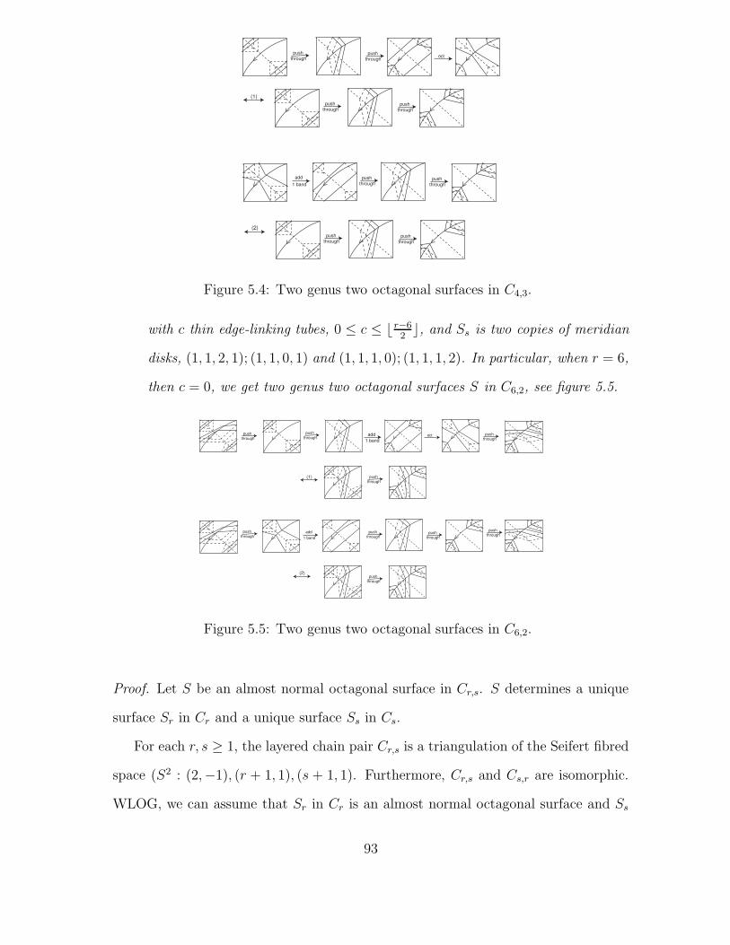
oct

(1)

pushadd

1 band through

push

through

push

through

push

through

push

throughpush

through

push

throughpush

through

(2)

Figure 5.4: Two genus two octagonal surfaces in C4,3.

with c thin edge-linking tubes, 0 ≤ c ≤ ⌊ r−62⌋, and Ss is two copies of meridian

disks, (1, 1, 2, 1); (1, 1, 0, 1) and (1, 1, 1, 0); (1, 1, 1, 2). In particular, when r = 6,

then c = 0, we get two genus two octagonal surfaces S in C6,2, see figure 5.5.

oct

(1)

pushadd

1 band throughpush

through

push

through

push

through

(2)

push

throughpush

through

push

through

push

through

add

1 band

push

through

Figure 5.5: Two genus two octagonal surfaces in C6,2.

Proof. Let S be an almost normal octagonal surface in Cr,s. S determines a unique

surface Sr in Cr and a unique surface Ss in Cs.

For each r, s ≥ 1, the layered chain pair Cr,s is a triangulation of the Seifert fibred

space (S2 : (2,−1), (r + 1, 1), (s + 1, 1). Furthermore, Cr,s and Cs,r are isomorphic.

WLOG, we can assume that Sr in Cr is an almost normal octagonal surface and Ss

93

in Cs is a normal surface, which is possibly disconnected.

Since Sr is an almost normal surface in the layered chain triangulation Cr, we can

list all the possible cases according to the theorem 5.1.

Case 1. Sr is an almost normal octagonal disk (possibly) with thin edge-linking

tubes.

1. Sr has edge-weight (2, 2, 2, 2); 2 × (1, 1, p′, p′ + 1), with p′ ≥ 1. This case is

impossible because according to the edge-weight matching equation 4.1,

(x, y, z, u); (x, y, v, z) ↔ (u, v, z, x); (u, v, y, z)

. we will have x = y = 2, u = 2, v = 2p′ and z = 2 = 2(p′ + 1). Hence, p′ = 0,

which contradicts to the fact that p′ ≥ 1.

2. Sr has edge-weight 2 × (1, 1, p + 1, p); (2, 2, 2, 2), with p ≥ 1. This case is

impossible because according to the edge-weight matching equation 4.1, we will

have x = y = 2, u = p, v = 2 and z = 2 = 2(p + 1). Hence, p = 0, which

contradicts to the fact that p′ ≥ 1.

3. Sr has edge-weight (2, 2, 2, 2) + (1, 1, p + 1, p); (1, 1, 0, 1) + 2× (1, 1, 1, 0), p ≥ 0.

This case is impossible because according to the edge-weight matching equation

4.1, we will have x = y = 3, u = 2 + p, v = 2 and z = 1 = 2 + p + 1. Hence,

p = −1,which contradicts to the fact that p′ ≥ 0.

4. Sr has edge-weight (2, 2, 2, 2)+(1, 1, p+1, p); (1, 1, p′+1, p′+2)+2×(1, 1, p′, p′+1),

p, p′ ≥ 0.

According to the edge-weight matching equation 4.1, we will have x = y = 3,

u = 2 + p, v = 3p′ + 1 and z = 2 + p + 1 = 3p′ + 4. Hence, p = 3p′ + 1.

We get v = p. Now the possible edge-weight for the normal surface Ss in

Cs is (u, v, z, x); (u, v, y, z) = (p + 2, p, p + 3, 3); (p + 2, p, 3, p + 3), which is

94

(2, 0, 1, 1) + (p, p, p + 2, 2); (2, 0, 1, 1) + (p, p, 2, p + 2). Notice for (p, p, p + 2, 2),

we have

(p, p, p + 2, 2) =

2 × (0, 0, 1, 1), p = 0

(1, 1, 3, 2), p = 1

2 × (1, 1, 2, 1), p = 2

2 × (1, 1, 2, 1) + (p − 2) × (1, 1, 1, 0), p ≥ 2

(5.2)

Notice for (p, p, 2, p + 2), we have

(p, p, 2, p + 2) =

2 × (0, 0, 1, 1), p = 0

(1, 1, 2, 3), p = 1

2 × (1, 1, 1, 2), p = 2

2 × (1, 1, 1, 2) + (p − 2) × (1, 1, 0, 1), p ≥ 2

(5.3)

Possibility 1. If p = 0, by p = 3p′ + 1 we get p′ is not integer, which is a

contradiction.

Possibility 2. If p = 1, P ′ = 0, since p = 3p′ + 1. Hence

Sr has edge-weight (2, 2, 2, 2) + (1, 1, 2, 1); (1, 1, 1, 2)+ 2× (1, 1, 0, 1). According

to the Case 2. 2(a) of the theorem 5.1. This is an octagonal disk and r = 3.

By the edge-weight matching equation 4.1, we have Ss in Cs has edge-weight

(2, 0, 1, 1) + (1, 1, 3, 2); (2, 0, 1, 1) + (1, 1, 2, 3). By theorem 2.2, we know that

there are two possibilities for Ss. First, it is a disjoint union of vertex-linking

disk (2, 0, 1, 1); (2, 0, 1, 1) and a meridian disk (1, 1, 3, 2); (1, 1, 2, 3). Hence we

get s = 5. After identifying the corresponding edges on ∂Sr and ∂Ss together,

we get an orientable almost normal octagonal surface S in C3,5. (2, 2, 2, 2) +

(1, 1, 2, 1); (1, 1, 1, 2)+2×(1, 1, 0, 1) ↔ (2, 0, 1, 1)+(1, 1, 3, 2); (2, 0, 1, 1)+(1, 1, 2, 3).

However, after identification, we notice this is a nonorientable surface. We ig-

nore it.

95

The other possibility for Ss is nonorientable surface from 6(b). Then the almost

normal S is obtained from this Ss is a nonorientable surface. Hence we ignore

it.

Possibility 3. If p = 2, by p = 3p′ + 1 we get p′ is not integer, which is a

contradiction.

Possibility 4. If p ≥ 2, we need to have 3|(p − 1), since p = 3p′ + 1 and p′ is

a nonnegative integer. Notice Ss has the edge-weight 2 × (1, 1, 2, 1) + (p − 2) ×

(1, 1, 1, 0); 2× (1, 1, 1, 2) + (p − 2) × (1, 1, 0, 1), when p ≥ 2.

Notice for any normal surfaces with bottom edge-weight 2×(1, 1, 2, 1)+(p−2)×

(1, 1, 1, 0) can only be obtained by pushing through. The change of edge-weight

after pushing through is showed as follows

2 × (1, 1, 2, 1) + (p − 2) × (1, 1, 1, 0)push−→ 2 × (1, 1, 1, 0) + (p − 2) × (1, 1, 0, 1)

push−→ 2 × (1, 1, 0, 1) + (p − 2) × (1, 1, 1, 2)

push−→ 2 × (1, 1, 1, 2) + (p − 2) × (1, 1, 2, 3)

push−→ · · ·

Since Ss has the top edge-weight 2×(1, 1, 1, 2)+(p−2)×(1, 1, 0, 1), when p ≥ 2.

We realize the only possibly case is when p−2 = 2, i.e. p = 4. In this case s = 2

and Ss is the disjoint union of two copies of meridian disk, (1, 1, 2, 1); (1, 1, 0, 1)

and two copies of meridian disk (1, 1, 1, 0); (1, 1, 1, 2) and vertex linking disk

(2, 0, 1, 1); (2, 0, 1, 1). Furthermore, when p = 4, p′ = 1. Hence Sr is octagonal

disk with edge-weight (2, 2, 2, 2)+(1, 1, 5, 4); (1, 1, 2, 3)+2×(1, 1, 1, 2), with r = 6.

Therefore, we get a almost octagonal normal surface S in C6,2. The matching

equation for Sr and Ss is (2, 2, 2, 2) + (1, 1, 5, 4); (1, 1, 2, 3) + 2 × (1, 1, 1, 2) ↔

2 × [(1, 1, 1, 2) + (1, 1, 0, 1)]. However, after identification, we notice this is a

nonorientable surface. We ignore it.

96

5. Sr has edge-weight 2× (1, 1, 0, 1)+(1, 1, 1, 0); (2, 2, 2, 2)+(1, 1, p′, p′+1), p′ ≥ 0.

It is impossible.

According to the edge-weight matching equation 4.1, we will have x = y = 3,

u = 2, v = p′ + 2 and z = 1 = p′ + 3. Hence, p′ = −2, which contradicts to the

fact that p′ ≥ 0.

6. Sr has edge-weight 2×(1, 1, p+1, p)+(1, 1, p+2, p+1); (2, 2, 2, 2)+(1, 1, p′, p′+1),

p, p′ ≥ 0.

According to the edge-weight matching equation 4.1, we will have x = y = 3, u =

3p+1, v = p′+2 and z = 3p+4 = p′+3. Hence, p′ = 3p+1 = u. Now the possible

edge-weight for the normal surface Ss in Cs is (u, v, z, x); (u, v, y, z) = (p′, p′ +

2, p′ +3, 3); (p′, p′ +2, 3, p′+3), which is (0, 2, 1, 1)+(p′, p′, p′ +2, 2); (0, 2, 1, 1)+

(p′, p′, 2, p′ + 2). According to the equations 4.5 and 4.6. we have the following

argument.

For (p′, p′, p′ + 2, 2), we have

(p′, p′, p′ + 2, 2) =

2 × (0, 0, 1, 1), p′ = 0

(1, 1, 3, 2), p′ = 1

2 × (1, 1, 2, 1), p′ = 2

2 × (1, 1, 2, 1) + (p′ − 2) × (1, 1, 1, 0), p′ ≥ 2

(5.4)

Notice for (p′, p′, 2, p′ + 2), we have

(p′, p′, 2, p′ + 2) =

2 × (0, 0, 1, 1), p′ = 0

(1, 1, 2, 3), p′ = 1

2 × (1, 1, 1, 2), p′ = 2

2 × (1, 1, 1, 2) + (p′ − 2) × (1, 1, 0, 1), p′ ≥ 2

(5.5)

Possibility 1. If p′ = 0, by p′ = 3p + 1 we get p is not integer, which is a

contradiction.

97

Possibility 2. If p′ = 1, P = 0, since p′ = 3p + 1. Hence

Sr has edge-weight 2 × (1, 1, 1, 0) + (1, 1, 2, 1); (2, 2, 2, 2) + (1, 1, 1, 2). Accord-

ing to the Case 2. 3(a) of the theorem 5.1. This is an octagonal disk and

r = 3. By the edge-weight matching equation 4.1, we have Ss in Cs has edge-

weight (0, 2, 1, 1) + (p′, p′, p′ + 2, 2); (0, 2, 1, 1) + (p′, p′, 2, p′ + 2) = (0, 2, 1, 1) +

(1, 1, 3, 2); (0, 2, 1, 1) + (1, 1, 2, 3). By theorem 2.2, we know that there are two

possibilities for Ss. First, it is a disjoint union of vertex-linking disk (0, 2, 1, 1);(0, 2, 1, 1)

and a meridian disk (1, 1, 3, 2); (1, 1, 2, 3). Hence we get s = 5.

After identifying the corresponding edges on ∂Sr and ∂Ss together, we get an

orientable almost normal octagonal surface S in C3,5. The matching equation

for Sr and Ss is 2× (1, 1, 1, 0)+(1, 1, 2, 1); (2, 2, 2, 2)+(1, 1, 1, 2) ↔ (0, 2, 1, 1)+

(1, 1, 3, 2); (0, 2, 1, 1)+ (1, 1, 2, 3) However, after identification, we notice this is

a nonorientable surface. We ignore it.

The other possibility for Ss is nonorientable surface from 6(b). Then the almost

normal S is obtained from this Ss is a nonorientable surface. Hence we ignore

it.

Possibility 3. If p′ = 2, by p′ = 3p + 1 we get p is not integer, which is a

contradiction.

Possibility 4. If p′ ≥ 2, we need to have 3|(p′ − 1), since p′ = 3p + 1 and p is

a nonnegative integer. Notice Ss has the edge-weight 2× (1, 1, 2, 1) + (p′ − 2)×

(1, 1, 1, 0); 2× (1, 1, 1, 2) + (p′ − 2) × (1, 1, 0, 1), when p ≥ 2.

Notice for any normal surfaces with bottom edge-weight 2×(1, 1, 2, 1)+(p′−2)×

(1, 1, 1, 0) can only be obtained by pushing through. The change of edge-weight

after pushing through is showed as follows

2 × (1, 1, 2, 1) + (p′ − 2) × (1, 1, 1, 0)push−→ 2 × (1, 1, 1, 0) + (p′ − 2) × (1, 1, 0, 1)

98

push−→ 2 × (1, 1, 0, 1) + (p′ − 2) × (1, 1, 1, 2)

push−→ 2 × (1, 1, 1, 2) + (p′ − 2) × (1, 1, 2, 3)

push−→ · · ·

Since Ss has the top edge-weight 2 × (1, 1, 1, 2) + (p′ − 2) × (1, 1, 0, 1), when

p ≥ 2. We realize the only possibly case is when p′ − 2 = 2, i.e. p′ = 4. In

this case s = 2 and Ss is the disjoint union of two copies of meridian disk,

(1, 1, 2, 1); (1, 1, 0, 1), two copies of meridian disk (1, 1, 1, 0); (1, 1, 1, 2) and two

copies of (0, 2, 1, 1); (0, 2, 1, 1). Furthermore, when p′ = 4, p = 1. Hence Sr is

octagonal disk with edge-weight 2×(1, 1, 2, 1)+(1, 1, 3, 2); (2, 2, 2, 2)+(1, 1, 4, 5),

with r = 6.

After identifying the corresponding edges on ∂Sr and ∂Ss together, we get an

orientable almost normal octagonal surface S in C6,2. The matching equation for

Sr and Ss is 2×(1, 1, 2, 1)+(1, 1, 3, 2); (2, 2, 2, 2)+(1, 1, 4, 5) ↔ 2× [(1, 1, 2, 1)+

(1, 1, 1, 0)]; 2× [(1, 1, 0, 1) + (1, 1, 1, 2)]. However, after identification, we notice

this is a nonorientable surface. We ignore it.

7. Sr has edge-weight (2, 2, 2, 2)+(1, 1, p+1, p); 2×(1, 1, 1, 0)+(1, 1, 2, 1), p ≥ 2. It

is impossible to get a S from this surface. According to the edge-weight matching

equation 4.1, we will have x = y = 3, u = 2 + p, v = 4 and z = p + 3 = 1.

Hence, p = −2, which contradicts to the fact that p ≥ 2.

8. Sr has edge-weight (2, 2, 2, 2)+(1, 1, p+1, p); 2×(1, 1, 0, 1)+(1, 1, 1, 0), p ≥ 2. It

is impossible to get a S from this surface. According to the edge-weight matching

equation 4.1, we will have x = y = 3, u = 2 + p, v = 1 and z = p + 3 = 2.

Hence, p = −1, which contradicts to the fact that p ≥ 2.

9. Sr has edge-weight (2, 2, 2, 2)+(1, 1, p+1, p); 2×(1, 1, p′+1, p′+2)+(1, 1, p′, p′+1),

p ≥ 2, p′ ≥ 0. According to the edge-weight matching equation 4.1, we will have

99

x = y = 3, u = 2 + p, v = 3p′ + 2 and z = p + 3 = 3p′ + 5. Hence,

p = 3p′+2 = v. Hence Ss has edge-weight (p+2, p, p+3, 3); (p+2, p, 3, p+3) =

(2, 0, 1, 1)+(p, p, p+2, 2); (2, 0, 1, 1)+(p, p, 2, p+2), p ≥ 2. According to equation

5.2, (p, p, p + 2, 2) = 2 × (1, 1, 2, 1) + (p − 2) × (1, 1, 1, 0) and (p, p, 2, p + 2) =

2 × (1, 1, 1, 2) + (p − 2) × (1, 1, 0, 1), with p ≥ 2.

Possibility 1. p = 2. Since p = 3p′ +2, we get p′ = 0. Hence, Sr is an octagonal

disk with edge-weight (2, 2, 2, 2)+(1, 1, 3, 2); 2×(1, 1, 1, 2)+(1, 1, 0, 1), with r = 3.

Ss has edge-weight (2, 0, 1, 1) + 2× (1, 1, 2, 1); (2, 0, 1, 1)+ 2× (1, 1, 1, 2). Hence

Ss is a disjoint union of vertex-linking disk (2, 0, 1, 1); (2, 0, 1, 1) and a normal

surface with edge-weight 2 × (1, 1, 2, 1); 2 × (1, 1, 1, 2). There are 3 possibilities

for this normal surface.

(a) If this normal surface is 2 copies of meridian disks, (1, 1, 2, 1); (1, 1, 1, 2),

with s = 3. After identifying the corresponding edges on ∂Sr and ∂Ss to-

gether, we get an orientable almost normal octagonal surface S in C3,3. The

matching equation for Sr and Ss is (2, 2, 2, 2) + (1, 1, 3, 2); 2× (1, 1, 1, 2) +

(1, 1, 0, 1) ↔ (2, 0, 1, 1)+2×(1, 1, 2, 1); (2, 0, 1, 1)+2×(1, 1, 1, 2). However,

after identification, we notice this is a nonorientable surface. We ignore

it.

(b) If this normal surface is an annulus (possibly ) with tubes, which is double

of nonorientable suface from 7(b.2) of theorem 2.2, (1, 1, 2, 1); (1, 1, 1, 2),

with s = 3 + 2c, c ≥ 0, which is the number of tetrahedron we add bands

in.

After identifying the corresponding edges on ∂Sr and ∂Ss together, we get

an orientable almost normal octagonal surface S in C3,3+2c. The matching

equation for Sr and Ss is (2, 2, 2, 2)+(1, 1, 3, 2); 2×(1, 1, 1, 2)+(1, 1, 0, 1) ↔

(2, 0, 1, 1)+ 2× (1, 1, 2, 1); (2, 0, 1, 1)+ 2× (1, 1, 1, 2). However, after iden-

100

tification, we notice this is a nonorientable surface. We ignore it.

(c) If this normal surface is an annulus (possibly ) with tubes from 7(c.4). Then

s ≥ 6. After identifying the corresponding edges on ∂Sr and ∂Ss together,

we get an orientable almost normal octagonal surface S in C3,3+2c. The

matching equation for Sr and Ss is (2, 2, 2, 2) + (1, 1, 3, 2); 2× (1, 1, 1, 2) +

(1, 1, 0, 1) ↔ (2, 0, 1, 1)+2×(1, 1, 2, 1); (2, 0, 1, 1)+2×(1, 1, 1, 2). However,

after identification, we notice this is a nonorientable surface. We ignore

it.

Possibility 2. For p ≥ 2, by the similar argument as in above case 4 possibility 4.

we have p− 2 = 2, i.e. p = 4 to have normal surface Ss. However, p = 3p′ + 2,

hence, p′ = 2/3, which is a contradiction.

10. Sr has edge-weight 2× (1, 1, 0, 1)+(1, 1, 1, 2); (2, 2, 2, 2)+(1, 1, p′, p′+1), p′ ≥ 2.

It is impossible to get an octagonal surface S. According to the edge-weight

matching equation 4.1, we will have x = y = 3, u = 4, v = p′ + 2 and z = 1 =

p′ + 3. Hence, p′ = −2, which is a contradiction to the fact p′ ≥ 2.

11. Sr has edge-weight 2 × (1, 1, 1, 0) + (1, 1, 0, 1); (2, 2, 2, 2) + (1, 1, p′, p′ + 1), p′ ≥

2.It is impossible to get an octagonal surface S. According to the edge-weight

matching equation 4.1, we will have x = y = 3, u = 1, v = p′ + 2 and z = 2 =

p′ + 3. Hence, p′ = −1, which is a contradiction to the fact p′ ≥ 2.

12. Sr has edge-weight 2×(1, 1, p+2, p+1)+(1, 1, p+1, p); (2, 2, 2, 2)+(1, 1, p′, p′+1),

p ≥ 0, p′ ≥ 2. According to the edge-weight matching equation 4.1, we will have

x = y = 3, u = 3p + 2, v = p′ + 2 and z = 3p + 5 = p′ + 3. Hence,

p′ = 3p + 2 = u, Now the possible edge-weight for the normal surface Ss in

Cs is (u, v, z, x); (u, v, y, z) = (p′, p′ + 2, p′ + 3, 3); (p′, p′ + 2, 3, p′ + 3), which is

(0, 2, 1, 1)+(p′, p′, p′+2, 2); (0, 2, 1, 1)+(p′, p′, 2, p′+2). The argument is similar

to the case [6.].

101

Possibility 1. If p′ = 0, by p′ = 3p + 2 we get p is not integer, which is a

contradiction.

Possibility 2. If p′ = 1,by p′ = 3p + 2 we get p is not integer, which is a

contradiction.

Possibility 3. If p′ = 2, by p′ = 3p + 2 we get p = 0. Now Sr is an octagonal

disk, 2× (1, 1, 2, 1) + (1, 1, 1, 0); (2, 2, 2, 2)+ (1, 1, 2, 3), with r = 3. Ss is a nor-

mal surface with edge-weight (u, v, z, x); (u, v, y, z) = (2, 4, 5, 3); (2, 4, 3, 5), i.e.

(0, 2, 1, 1)+2×(1, 1, 2, 1); (0, 2, 1, 1)+2×(1, 1, 1, 2). There are three possibilities

for Ss.

(a) If this normal surface is a disjoint union of vertex-linking disk, (0, 2, 1, 1);(0, 2, 1, 1),

and 2 copies of meridian disks, (1, 1, 2, 1); (1, 1, 1, 2), with s = 3.

After identifying the corresponding edges on ∂Sr and ∂Ss together, we get

an orientable almost normal octagonal surface S in C3,3. . The matching

equation for Sr and Ss is 2×(1, 1, 2, 1)+(1, 1, 1, 0); (2, 2, 2, 2)+(1, 1, 2, 3) ↔

(0, 2, 1, 1)+ 2× (1, 1, 2, 1); (0, 2, 1, 1)+ 2× (1, 1, 1, 2). However, after iden-

tification, we notice this is a nonorientable surface. We ignore it.

(b) If this normal surface is a disjoint union of vertex-linking disk, (0, 2, 1, 1);(0, 2, 1, 1),

and an annulus (possibly ) with tubes, which is double of nonorientable su-

face from 7(b.2) of theorem 2.2, (1, 1, 2, 1); (1, 1, 1, 2), with s = 3 + 2c,

c ≥ 0, with c ≥ 1.

After identifying the corresponding edges on ∂Sr and ∂Ss together, we get

an orientable almost normal octagonal surface S in C3,3+2c, with c ≥ 1.

The matching equation for Sr and Ss is 2×(1, 1, 2, 1)+(1, 1, 1, 0); (2, 2, 2, 2)+

(1, 1, 2, 3) ↔ (0, 2, 1, 1)+2×(1, 1, 2, 1); (0, 2, 1, 1)+2×(1, 1, 1, 2). However,

after identification, we notice this is a nonorientable surface. We ignore

it.

102

(c) If this normal surface is an annulus (possibly) with tubes from 7(c.4). Then

s ≥ 6. After identifying the corresponding edges on ∂Sr and ∂Ss to-

gether, we get an orientable almost normal octagonal surface S in C3,s,

with s ≥ 6. The matching equation for Sr and Ss is 2 × (1, 1, 2, 1) +

(1, 1, 1, 0); (2, 2, 2, 2)+ (1, 1, 2, 3) ↔ (0, 2, 1, 1) + 2× (1, 1, 2, 1); (0, 2, 1, 1)+

2×(1, 1, 1, 2) However, after identification, we notice this is a nonorientable

surface. We ignore it.

Possibility 4. If p′ ≥ 2, we need to have 3|(p′ − 2), since p′ = 3p + 2 and p is

a nonnegative integer. By the similar argument we have in case [6.] We must

have p′ − 2 = 2 in order to have a corresponding normal surface Ss. Then this

contradicts to the fact 3|(p′ − 2). Therefore, this is impossible.

Case 2. Sr is an almost normal octagonal annulus (possibly) with thin edge-linking

tubes.

1. Sr has edge-weight 2×(1, 1, p+1, p); 2×(1, 1, p′, p′+1), p ≥ 0,p′ ≥ 1. According

to the edge-weight matching equation 4.1,

(x, y, z, u); (x, y, v, z) ↔ (u, v, z, x); (u, v, y, z)

we will have x = y = 2, u = 2p, v = 2p′ and z = 2(p + 1) = 2(p′ + 1). Hence,

p = p′ and p ≥ 1.

Now the possible edge-weight for the normal surface Ss in Cs is (u, v, z, x); (u, v, y, z) =

(2p, 2p, 2p + 2, 2); (2p, 2p, 2, 2p + 2).

For the bottom edge-weight (2p, 2p, 2p+ 2, 2), according to the equation 4.5 we

have

(2p, 2p, 2p + 2, 2) =

2 × (0, 0, 1, 1), p = 0

2 × (1, 1, 2, 1), p = 1

2 × (1, 1, 2, 1) + (2p − 2)(1, 1, 1, 0), p ≥ 2

(5.6)

103

For the top edge-weight (2p, 2p, 2, 2p+2),according to the equation 4.6 we have

(2p, 2p, 2, 2p + 2) =

2 × (0, 0, 1, 1), p = 0

2 × (1, 1, 1, 2), p = 1

2 × (1, 1, 1, 2) + (2p − 2)(1, 1, 0, 1), p ≥ 2

(5.7)

Since p = p′ ≥ 1 Possibility 1. If p = 1, then p′ = p = 1. we have Sr is

an octagonal annulus (possibly) with c thin edge-linking tubes,2× (1, 1, 2, 1); 2×

(1, 1, 1, 2). Then r ≥ 4, since it needs at least 3 steps from the edge-weight

2 × (1, 1, 2, 1) to (2, 2, 2, 2), and one more step to add an octagonal disk to get

a surface with top edge-weight 2 × (1, 1, 1, 2). Moreover, we will have Ss has

edge-weight 2× (1, 1, 2, 1); 2× (1, 1, 1, 2). There are three possible choices for Ss.

(a) If Ss is a normal surface of two copies of meridian disks, 2×(1, 1, 2, 1); 2×

(1, 1, 1, 2). We notice s = 3. After identifying the corresponding edges on

∂Sr and ∂Ss together, we get an orientable almost normal octagonal surface

S with genus c + 2 in Cr,3, where r ≥ 4. In particular, if r = 4, we get a

genus 2 orientable octagonal surface S in C4,3. Later, we will show that it

is a Heegaard splitting. The matching equation for Sr and Ss is

2 × (1, 1, 2, 1); 2× (1, 1, 1, 2) ↔ 2 × (1, 1, 2, 1); 2× (1, 1, 1, 2)

(b) If Ss is an annulus (possibly ) with c′ thin edge-linking tubes, which is

double of nonorientable suface from 7(b.2) of theorem 2.2, 2×(1, 1, 2, 1); 2×

(1, 1, 1, 2), with s = 3 + 2c′.

After identifying the corresponding edges on ∂Sr and ∂Ss together, we get

an orientable almost normal octagonal surface S with genus c + c′ + 3 in

Cr,3+2c′, r ≥ 4. The matching equation for Sr and Ss is

2 × (1, 1, 2, 1); 2× (1, 1, 1, 2) ↔ 2 × (1, 1, 2, 1); 2× (1, 1, 1, 2)

104

(c) If this normal surface is an annulus (possibly ) with tubes from 7(c.4). Then

s ≥ 6. After identifying the corresponding edges on ∂Sr and ∂Ss together,

we get an orientable almost normal octagonal surface S with genus 3+c+c′

in Cr,s, where r ≥ 4 and s ≥ 6. The matching equation for Sr and Ss is

2 × (1, 1, 2, 1); 2× (1, 1, 1, 2) ↔ 2 × (1, 1, 2, 1); 2× (1, 1, 1, 2)

Possibility 2. If p ≥ 2. Ss has edge-weight 2× (1, 1, 2, 1)+(2p−2)(1, 1, 1, 0); 2×

(1, 1, 1, 2) + (2p − 2)(1, 1, 0, 1). Notice

2 × (1, 1, 2, 1) + (2p − 2)(1, 1, 1, 0)push−→ 2 × (1, 1, 1, 0) + (2p − 2) × (1, 1, 0, 1)

push−→ 2 × (1, 1, 0, 1) + (2p − 2) × (1, 1, 1, 2)

push−→ 2 × (1, 1, 1, 2) + (2p − 2) × (1, 1, 2, 3)

push−→ · · ·

Compare this with the top edge-weight 2× (1, 1, 1, 2) + (2p− 2)(1, 1, 0, 1) of Ss.

The only possible choice for p is 2p − 2 = 2, which p = 2.

When p = 2, p′ = p = 2. we have Sr is an octagonal annulus (possibly)

with c thin edge-linking tubes, 2 × (1, 1, 3, 2); 2 × (1, 1, 2, 3).Then r ≥ 6, since

it needs at least 4 steps from the edge-weight 2 × (1, 1, 2, 1) to (2, 2, 2, 2), a

step to add an octagonal disk and one more step to push through the surface to

get top edge-weight 2 × (1, 1, 2, 3). Moreover, we will have Ss has edge-weight

2× (1, 1, 2, 1)+2× (1, 1, 1, 0); 2× (1, 1, 1, 2)+2× (1, 1, 0, 1). Hence, Ss can only

obtained two copies of disconnected normal meridian disks, (1, 1, 2, 1); (1, 1, 0, 1)

and (1, 1, 1, 0); (1, 1, 1, 2). Therefore, s = 2

After identifying the corresponding edges on ∂Sr and ∂Ss together, we get an

orientable almost normal octagonal surface S with genus 2 + c in Cr,2, r ≥ 6.

The matching equation for Sr and Ss is

2×(1, 1, 3, 2); 2×(1, 1, 2, 3) ↔ 2×(1, 1, 2, 1)+2×(1, 1, 1, 0); 2×(1, 1, 1, 2)+2×(1, 1, 0, 1)

105

In particular, when in C6,2, we will have an orientable octagonal surface with

genus two, this is the Heegaard splitting surface.

2. Sr has edge-weight 2 × (1, 1, 0, 1); 2 × (1, 1, p′, p′ + 1), p′ ≥ 1. It is impossible,

because according to the edge-weight matching equation 4.1, we will have x =

y = 2, u = 2, v = 2p′ and z = 0 = 2(p′ + 1). Hence, p′ = −1, which is a

contradiction to the fact that p′ ≥ 1.

3. Sr has edge-weight 2×(1, 1, p+1, p); 2×(1, 1, p′, p′+1), p ≥ 1,p′ ≥ 0. This edge-

weight is the same as the case [1.], except the domain of p and p′. According to

the edge-weight matching equation 4.1, we will have x = y = 2, u = 2p, v = 2p′

and z = 2(p+1) = 2(p′+1). Hence, p = p′ and p ≥ 1. Therefore, the discussion

is exactly follow the first case in Case 2.

Possibility 1. If p = 1, then p′ = p = 1. we have Sr is an octagonal annulus

(possibly) with c thin edge-linking tubes,2× (1, 1, 2, 1); 2× (1, 1, 1, 2), with r ≥ 4.

There are three possible choices for Ss.

(a) If Ss is a normal surface of two copies of meridian disks, 2×(1, 1, 2, 1); 2×

(1, 1, 1, 2), with s = 3. After identifying the corresponding edges on ∂Sr

and ∂Ss together, we get an orientable almost normal octagonal surface S

with genus c + 2 in Cr,3, where r ≥ 4. In particular, if r = 4, we get a

genus two orientable octagonal surface S in C4,3. Later, we will show that

it is a Heegaard splitting. The matching equation for Sr and Ss is

2 × (1, 1, 2, 1); 2× (1, 1, 1, 2) ↔ 2 × (1, 1, 2, 1); 2× (1, 1, 1, 2)

(b) If Ss is an annulus (possibly ) with c′ thin edge-linking tubes, which is

double of nonorientable suface from 7(b.2) of theorem 2.2, 2×(1, 1, 2, 1); 2×

(1, 1, 1, 2), with s = 3 + 2c′.

106

After identifying the corresponding edges on ∂Sr and ∂Ss together, we get

an orientable almost normal octagonal surface S with genus c + c′ + 3 in

Cr,3+2c′, r ≥ 4. The matching equation for Sr and Ss is

2 × (1, 1, 2, 1); 2× (1, 1, 1, 2) ↔ 2 × (1, 1, 2, 1); 2× (1, 1, 1, 2)

(c) If this normal surface is an annulus (possibly ) with tubes from 7(c.4). Then

s ≥ 6. After identifying the corresponding edges on ∂Sr and ∂Ss together,

we get an orientable almost normal octagonal surface S with genus 3+c+c′

in Cr,s, where r ≥ 4 and s ≥ 6. The matching equation for Sr and Ss is

2 × (1, 1, 2, 1); 2× (1, 1, 1, 2) ↔ 2 × (1, 1, 2, 1); 2× (1, 1, 1, 2)

Possibility 2. If p = 2, p′ = p = 2. we have Sr is an octagonal annulus (possibly)

with c thin edge-linking tubes, 2×(1, 1, 3, 2); 2×(1, 1, 2, 3), with r ≥ 6. Moreover,

we will have Ss has edge-weight 2 × (1, 1, 2, 1) + 2 × (1, 1, 1, 0); 2× (1, 1, 1, 2) +

2 × (1, 1, 0, 1). Hence, Ss can only obtained two copies of disconnected normal

meridian disks, (1, 1, 2, 1); (1, 1, 0, 1) and (1, 1, 1, 0); (1, 1, 1, 2). Therefore, s = 2

After identifying the corresponding edges on ∂Sr and ∂Ss together, we get an

orientable almost normal octagonal surface S with genus 2 + c in Cr,2, r ≥ 6.

The matching equation for Sr and Ss is 2 × (1, 1, 3, 2); 2 × (1, 1, 2, 3) ↔ 2 ×

(1, 1, 2, 1) + 2 × (1, 1, 1, 0); 2× (1, 1, 1, 2) + 2 × (1, 1, 0, 1) In particular, when in

C6,2, we will have an orientable octagonal surface with genus two, this is the

Heegaard splitting surface.

4. Sr has edge-weight 2 × (1, 1, p + 1, p); 2 × (1, 1, 1, 0), p ≥ 1. It is impossible.

According to the edge-weight matching equation 4.1, we will have x = y = 2,

u = 2p, v = 2 and z = 2(p + 1) = 0. Hence p = −1, which contradicts to the

fact that p ≥ 1.

107

5. Sr has edge-weight (1, 1, 1, 0) + (1, 1, 0, 1); (1, 1, p′, p′ + 1) + (1, 1, p′ + 1, p′ + 2),

p′ ≥ 0. It is impossible. According to the edge-weight matching equation 4.1,

we will have x = y = 2, u = 1, v = 2P ′ + 1 and z = 1 = 2P ′ + 3. Hence

p′ = −1,which contradicts to the fact that p′ ≥ 0.

6. Sr has edge-weight (1, 1, p + 2, p + 1) + (1, 1, p + 1, p); (1, 1, 1, 0) + (1, 1, 0, 1),

p ≥ 0. It is impossible. According to the edge-weight matching equation 4.1, we

will have x = y = 2, u = 2p+1, v = 1 and z = 2P +3 = 1. Hence p = −1,which

contradicts to the fact that p ≥ 0.

7. Sr has edge-weight (1, 1, p+ 2, p+ 1) + (1, 1, p+ 1, p); (1, 1, p′, p′ + 1) + (1, 1, p′ +

1, p′ + 2), p ,p′ ≥ 0. According to the edge-weight matching equation 4.1, we

will have x = y = 2, u = 2p + 1, v = 2p′ + 1 and z = 2P + 3 = 2p′ + 3.

Hence p = p′. Now the possible edge-weight for the normal surface Ss in Cs is

(u, v, z, x); (u, v, y, z) = (2p + 1, 2p + 1, 2p + 3, 2); (2p + 1, 2p + 1, 2, 2p + 3).

For the bottom edge-weight (2p + 1, 2p + 1, 2p + 3, 2), according to the equation

4.5 we have

(2p + 1, 2p + 1, 2p + 3, 2) =

((1, 1, 3, 2), p = 0

2 × (1, 1, 2, 1) + (2p − 1)(1, 1, 1, 0), p ≥ 1(5.8)

For the top edge-weight (2p + 1, 2p + 1, 2, 2p + 3),according to the equation 4.6

we have

(2p, 2p, 2, 2p + 2) =

(1, 1, 3, 2), p = 0

2 × (1, 1, 1, 2) + (2p − 1)(1, 1, 0, 1), p ≥ 1(5.9)

Possibility 1. If p = 0, then p′ = p = 0. we have Sr is an octagonal annulus

(with no tubes), (1, 1, 2, 1) + (1, 1, 1, 0); (1, 1, 0, 1) + (1, 1, 1, 2). Notice r = 3,

because

(1, 1, 2, 1) + (1, 1, 1, 0)push−→ (1, 1, 1, 0) + (1, 1, 0, 1)

108

oct−→ (1, 1, 1, 0) + (1, 1, 0, 1)

push−→ (1, 1, 0, 0) + (1, 1, 1, 2)

Furthermore, the possible edge-weight for the normal surface Ss in Cs is (u, v, z, x); (u, v, y, z)=

(1, 1, 3, 2); (1, 1, 2, 3). There are two possible choices for Ss.

(a) Ss is a copy of meridian disk, (1, 1, 3, 2); (1, 1, 2, 3). Then we get s = 5.

After identifying the corresponding edges on ∂Sr and ∂Ss together, we get

an orientable almost normal octagonal surface S in C3,5.

The matching equation for Sr and Ss is

(1, 1, 2, 1) + (1, 1, 1, 0); (1, 1, 0, 1) + (1, 1, 1, 2) ↔ (1, 1, 3, 2); (1, 1, 2, 3)

However, after identification, we notice this is a nonorientable surface. We

ignore it.

(b) Ss is a nonorientable surface,(1, 1, 3, 2); (1, 1, 2, 3). This will give us a

nonorientable octagonal S after identifying the corresponding edges on ∂Sr

and ∂Ss together. Therefore, we will ignore this case.

Possibility 2. If p ≥ 1, since

2 × (1, 1, 2, 1) + (2p − 1)(1, 1, 1, 0)push−→ 2 × (1, 1, 1, 0) + (2p − 1) × (1, 1, 0, 1)

push−→ 2 × (1, 1, 0, 1) + (2p − 1) × (1, 1, 1, 2)

push−→ 2 × (1, 1, 1, 2) + (2p − 2) × (1, 1, 2, 3)

push−→ · · ·

Therefore, if we need to find a surface Ss with edge-weight (2p + 1, 2p + 1, 2p +

3, 2); (2p + 1, 2p + 1, 2, 2p + 3) for p ≥ 1, it requires that 2p − 1 = 2, hence p is

not an integer. Therefore it is impossible.

109

8. Sr has edge-weight(2, 2, 2, 2)+(0, 0, 1, 1); (1, 1, 2, 1)+(1, 1, 1, 0). It is impossible.

According to the edge-weight matching equation 4.1, we will have x = y = 2,

u = 3, v = 3 and z = 3 = 1, which is impossible.

9. Sr has edge-weight(2, 2, 2, 2)+(0, 0, 1, 1); (1, 1, 1, 0)+(1, 1, 0, 1). It is impossible.

According to the edge-weight matching equation 4.1, we will have x = y = 2,

u = 3, v = 1 and z = 3 = 1, which is impossible.

10. Sr has edge-weight(2, 2, 2, 2) + (0, 0, 1, 1); (1, 1, p′, p′ + 1) + (1, 1, p′ + 1, p′ + 2),

p′ ≥ 0. According to the edge-weight matching equation 4.1, we will have x =

y = 2, u = 3, v = 2p′ + 1 and z = 3 = 2p′ + 3. Hence p′ = 0. Sr has

edge-weight(2, 2, 2, 2) + (0, 0, 1, 1); (1, 1, 0, 1) + (1, 1, 1, 2), with r ≥ 3, since

(2, 2, 2, 2) + (0, 0, 1, 1)push−→ · · ·

push−→ (2, 2, 2, 2) + (0, 0, 1, 1)

oct−→ (1, 1, 2, 1) + (1, 1, 1, 0)

push−→ (1, 1, 1, 0) + (1, 1, 0, 1)

push−→ (1, 1, 0, 1) + (1, 1, 1, 2)

Now the possible edge-weight for the normal surface Ss in Cs is (u, v, z, x); (u, v, y, z) =

(3, 1, 3, 2); (3, 1, 2, 3) = (2, 0, 1, 1)+ (1, 1, 2, 1); (2, 0, 1, 1)+ (1, 1, 1, 2). Therefore,

there are two possible choices for Ss.

(a) Ss is a disjoint union of vertex-linking disk, (2, 0, 1, 1); (2, 0, 1, 1) and a

meridian disk (1, 1, 2, 1); (1, 1, 1, 2). Notice here s = 3. After identifying

the corresponding edges on ∂Sr and ∂Ss together, we get an orientable

almost normal octagonal surface S in Cr,3, r ≥ 3.

The matching equation for Sr and Ss is (2, 2, 2, 2)+ (0, 0, 1, 1); (1, 1, 0, 1)+

(1, 1, 1, 2) ↔ (2, 0, 1, 1) + (1, 1, 2, 1); (2, 0, 1, 1) + (1, 1, 1, 2). However, this

is a nonorientable surface. We ignore it.

110

(b) Ss is a disjoint union of vertex-linking disk, (2, 0, 1, 1); (2, 0, 1, 1) and a

nonorientable surface (1, 1, 2, 1); (1, 1, 1, 2). Then after identifying the cor-

responding edges on ∂Sr and ∂Ss together, we get a nonorientable octagonal

surface. We ignore this case.

11. Sr has edge-weight(1, 1, 0, 1) + (1, 1, 1, 2); (2, 2, 2, 2) + (0, 0, 1, 1). This case is

impossible. According to the edge-weight matching equation 4.1, we will have

x = y = 2, u = 3, v = 3 and z = 1 = 3, which is impossible.

12. Sr has edge-weight(1, 1, 1, 0) + (1, 1, 0, 1); (2, 2, 2, 2) + (0, 0, 1, 1). This case is

impossible. According to the edge-weight matching equation 4.1, we will have

x = y = 2, u = 1, v = 3 and z = 1 = 3, which is impossible.

13. Sr has edge-weight(1, 1, p+2, p+1)+(1, 1, p+1, p); (2, 2, 2, 2)+(0, 0, 1, 1), p ≥ 0.

According to the edge-weight matching equation 4.1, we will have x = y = 2,

u = 2p + 1, v = 3 and z = 2p + 3 = 3. Hence we get p = 0. Hence Sr has

edge-weight (1, 1, 2, 1) + (1, 1, 1, 0); (2, 2, 2, 2) + (0, 0, 1, 1). Notice here r ≥ 3

(1, 1, 2, 1) + (1, 1, 1, 0)push−→ (1, 1, 1, 0) + (1, 1, 0, 1)

push−→ (1, 1, 0, 1) + (1, 1, 1, 2)

oct−→ (2, 2, 2, 2) + (0, 0, 1, 1)

push−→ cdots

push−→ (2, 2, 2, 2) + (0, 0, 1, 1)

Now the possible edge-weight for the normal surface Ss in Cs is (u, v, z, x); (u, v, y, z)=

(1, 3, 3, 2); (1, 3, 2, 3) = (0, 2, 1, 1)+ (1, 1, 2, 1); (0, 2, 1, 1)+ (1, 1, 1, 2). Therefore,

there are two possible choices for Ss.

(a) Ss is a disjoint union of vertex-linking disk, (0, 2, 1, 1); (0, 2, 1, 1) and a

meridian disk (1, 1, 2, 1); (1, 1, 1, 2). Notice here s = 3. After identifying

the corresponding edges on ∂Sr and ∂Ss together, we get an orientable

111

almost normal octagonal surface S in Cr,3, r ≥ 3. The matching equation

for Sr and Ss is (1, 1, 2, 1)+(1, 1, 1, 0); (2, 2, 2, 2)+(0, 0, 1, 1) ↔ (0, 2, 1, 1)+

(1, 1, 2, 1); (0, 2, 1, 1)+(1, 1, 1, 2). However, this is a nonorientable surface.

We ignore it.

(b) Ss is a disjoint union of vertex-linking disk, (0, 2, 1, 1); (0, 2, 1, 1) and a

nonorientable surface (1, 1, 2, 1); (1, 1, 1, 2). Then after identifying the cor-

responding edges on ∂Sr and ∂Ss together, we get a nonorientable octagonal

surface. We ignore this case.

Let’s consider the smallest genus octagonal surfaces in each layered chain pair

triangulation of Mr,s. We notice according to theorem 5.3, this happens if and only

if c = c′ = 0.

Corollary 5.1 The octagonal almost normal surface with the smallest genus in the

layered chain triangulation of Mr,s,r, s ≥ 2 are isotopic to one of the followings,

1. In Cn,3 = C3,n, n ≥ 5, there are only two almost normal octagonal surfaces of

genus 2.

2. In Cr,2 = C2,r, r ≥ 6, there are only two almost normal octagonal surfaces with

genus 2.

3. In Cr,s = Cs,r, r, s ≥ 5 or C4,5 = C5,4, all the almost normal octagonal surfaces

has genus at least 3.

4. There is no octagonal surface in other C(r, s). The list of them are C3,3, C4,4,

C2,s = Cs,2, 2 ≤ s ≤ 5.

All in all, there are almost normal octagonal surfaces in any layered chain pair

triangulation Cr,s of Mr,s, except for M2,2, M2,3, M2,4, M2,5, M3,3 and M4,4. Notice the

first 5 Seifert fibered manifolds satisfies the condition∑

1/αi ≥ 1, with i = 1, 2, 3.

112

We also notice that M4,3 = M3,4=W (2, 4, b), where b = 5, and M2,6 = M6,2=V (2, 3, a),

where a = 7.

1. V (2, 3, a) is a Brieskon manifold.

V (2, 3, a) ={z ∈ C3|z12 + z2

3 + z3a = 0, ‖z‖ = 1}, with 3 ∤ a, a ≥ 7.

If a is even, V (2, 3, a) = S(0;− 16a

; 12, (−a)−1

3, 6−1

a), otherwise

V (2, 3, 2a′)=S(0;− 13a

; −a′−1

3, −a′−1

3, 3−1

a′),

2. W (2, 4, b) is the link of the singularity.

W (2, 4, b)={z ∈ C3|z12 + (z2

2 + z3b)z2 = 0, ‖z‖ = 1}, with 2 ∤ b, b ≥ 5

W (2, 4, b) = S(0;− 14b

; 12, (−b)−1

4, 4−1

b).

In fact, by comparing the seifert invariant notations of Mr,s with V (2, 3, a) and

W (2, 4, b). We notice M4,3 = M3,4 and M2,6 = M6,2 are the only two manifolds in

Mr,s belongs to these two special families of manifolds.

113

CHAPTER 6

Heegaard splitting surfaces

In this chapter, we will discuss Heegaard splitting surfaces in twisted layered loop

triangulations of Seifert fibred spaces Mk = S3/Q4k = S2((2, 1), (2, 1)(k, 1 − k)),

and layered chain pairs triangulation of Seifert fibred space Mr,s=(S2 : (2,−1), (r +

1, 1), (s + 1, 1)), respectively.

Definition 6.1 In the twisted layered loop triangulation Ck of the manifold M , if

we cut the triangulation along a level annulus that meets a thin edge-linking tube,

which is not t = b, then M turns into a solid torus, and the twisted layered loop

triangulation turns into the layered chain triangulation. Furthermore, the boundaries

of this thin edge-linking tube in M will separate the torus boundary into two annulus.

The annulus which contains the vertices is called the companion annulus for this tube.

The other annulus is called the complementary annulus.

There are two possible companion/complementary annulus for the same thin edge-

linking tube. It depends where we cut the level annulus. See figure 6.1

Definition 6.2 If an almost normal tubed surface is obtained by adding an almost

normal tube to a normal surface along an edge, which intersects with some quad(s) of

a thin edge-linking tube from this normal surface, it is called an almost normal tubed

surface with the almost normal tube at the same level of a thin edge-linking tube.

114

push

thro

ugh

pushthrough

pushthrough

push

thro

ugh

Postition 1 Position 2

Figure 6.1: The complementary annuli w.r.t. a thin edge-linking tube.

6.1 Heegaard splitting surfaces in the twisted layered loop

triangulations

.

In this section we will show that Heegaard splitting surface can not be normal in

the twisted layered loop triangulation of M . Moreover, we will discuss what surfaces

are Heegaard splitting surfaces and answer the classification problem for Heegaard

splitting surfaces.

Theorem 6.1 Any orientable normal surface in the twisted layered loop triangulation

of small Seifert fibred space M is not Heegaard splitting surface.

Proof. First notice that any orientable normal surface in twisted layered loop triangu-

lation is a vertex-linking 2-sphere (possibly) with thin edge-linking tubes by theorem

3.1.

The manifold M is a small Seifert fibered space, not S3 or lens space. According

to the papers [33], M can not have genus 0 or 1 Heegaard splittings. Therefore, we

only consider the normal surface S2 with at least two thin edge-linking tubes.

Let S be a normal surface, a vertex-linking disk with at least two thin edge-linking

tubes. We assume that S has genus g, then g ≥ 2. We will prove this theorem by

115

contradiction.

Suppose S is a Heegaard splitting surface of M . S separates M into 2 handlebodies

H , H ′.

Let H be the handlebody containing the unique vertex of the twisted layered loop

triangulation Ck. Then H is a handlebody. If we cut M along a level annulus that

meets a thin edge-linking tube, then S become a normal surface S ′, an annulus with

at least one tube in the layered chain triangulation of the solid torus M . S ′ has a

companion annulus A and a complementary annulus B on the boundary of the solid

torus M .

Let’s first make an observation. Notice B is an embedded Mobius band in the

handlebody H ′ before cutting. This is because t = −b and B is doesn’t contains

vertice and B ∩ H=B ∩ ∂H=B ∩ S=∂B(=∂A). Since any embedded surface in a

handlebody is compressible or ∂-compressible in H ′.

First we will show that Mobius band is not compressible. Let γ be a noncon-

tractable simple closed curve on the Mobius band. This curve is orientation reversing

curve. Suppose that we can find a compression disk for this Mobius and ∂D is γ.

Let’s take the small regular neighborhood of D, we get a ball with curve γ on its

boundary. Since γ is orientation reversing curve, the small regular neighborhood of

it on the 2-sphere is a Mobius band. Furthermore, any simple closed curve on the

2-sphere bounds a disk. Hence, we can add a disk on the boundary of this Mobius,

therefore, we get a RP2 on the surface 2-sphere, which is impossible because the first

homology of RP2 is Z2, which can not be a subgroup of Z. Mobius band is therefore

not compressible.

Mobius band is ∂-compressible in a handlebody. Now let’s consider all ∂-compressing

disks for all possible Mobius bands Bs in the handlebody H ′.

Let D be a ∂-compressing disk for the some Mobius band B with respect to thin

edge-linking tube e, where −b 6= e 6= t, so that it has minimal intersection with all

116

the Bs in H ′, where ∂D ∩ S = α, ∂D ∩ B = β, and ∂D = α ∪ β.Notice D ⊂ H ′.

Let’s first consider the case if there is an innermost simple closed intersection

curve in D.

Notice this simple closed curve can only be a trivial curve. Otherwise, it is an

orientation reversing curve on the Mobius band, we know it cannot bounds a disk

here. If it is a trivial curve in some B′, then we can use standard techniques to modify

the intersection to reduce the number of intersection components in D, Since every S2

bounds a ball in an irreducible manifold. Therefore, we get a new ∂-compressing disk

for the annulus B which has less intersection with the collection of the complementary

annuli. This is a contradiction to the fact that D has the minimal intersection with

the collection of complementary annuli. It is impossible.

Now Let’s consider the outermost intersection arc in D with the collection of

complementary annuli .

If it is a trivial arc in some B′, it will cobound a disk with an arc γ on the boundary

of B′. Moreover, this trivial arc will separate ∂D into two parts, and obviously that

the two endpoints of the arc are on the boundary of B′ ⊂ S, hence they are in the arc

α. Now we can construct a new ∂-compressing disk D′ for B, where ∂D′ = β ∪ γ∪

the two segments on the ∂D between the endpoints of γ and β.

If it is an essential arc, denoted by γ in some B′. we will get a new ∂-compressing

disk D′ for B′, with ∂D′ is the union of γ and the arc which is the segment in α ⊂ S

obtained by separation from the endpoints of γ on the ∂D. Obviously D′ ⊂ D

has less intersection with the collection of complementary annuli for S. This is a

contradiction.

Therefore, the ∂-compressing disk D for the Mobius band B in H ′ doesn’t intersect

with any other Mobius band Bs with respect to other thin edge-linking tubes.

Furthermore, we get that D is also a ∂-compressing disk for the annulus with

respect to edge e of the normal surface S ′ into its complementary annulus B on the

117

boundary of the layered chain triangulation of the solid torus. First we notice that

β ⊂ B has two endpoints on two different boundaries of B in the layered chain

triangulation. Therefore, it is essential arc on the annulus B. Moreover, α ⊂ S is an

arc on the annulus part of S ′ without hitting other tubes and it have same endpoints

as β. Therefore, α is an arc with endpoints on the different boundaries of the annulus

of S with respect to the thin edge-linking tube e. Therefore, We get that α is essential

with respect to the thin edge-linking tube e. Therefore, We get the annulus of S ′ with

respect to thin edge-linking tube e is ∂-compressed to its complementary annulus B,

and D is a ∂-compressing disk in the solid torus. Therefore, the companion annulus

of the annulus in S ′ is ∂-compressed into its the complementary annulus. Hence, the

thin edge that the annulus is around should be longitudinal. However, this edge e is

not t or b. This is a contradiction.

Therefore, no normal surface in the twisted layered loop triangulation is a Hee-

gaard splitting surface.

Lemma 6.1 If S is an almost normal tubed surface which is obtained by adding an

almost normal tube between two connected normal surfaces in the twisted layered loop

triangulation, then S can not be a Heegaard splitting surface.

Proof. Let S be an almost normal surface which is obtained by adding an almost

normal tube between two compatible connected normal surfaces S1 and S2 in the

twisted layered loop triangulation. Furthermore, S1 separates S2 from the vertex.

Obviously, S1 and S2 are both vertex-linking S2 (possibly) with thin edge-linking

tubes by theorem 3.1. They all bounds a handlebody on the side which contains

the unique vertex in the twisted layered loop triangulation of M . We will prove the

theroem by contradiction.

Let’s assume that S is a Heegaard Splitting surface. S separates M into two

118

handlebodies H and H ′, where H is the one that contains the vertex. Then S2 is

a disk connected summand of S and it bounds a handlebody that is a connected

summand of H on the side that not only doesn’t contain the vertex, but also is

disjoint from S1. Hence, S2 boundsa handlebody on both sides. Therefore, it is a

Heegaard splitting surface. However, According to the theorem 6.1, no normal surface

can be a Heegaard splitting surface. This is a contradiction. Therefore, S can not be

a Heegaard splitting surface.

Now we will come to answwer the question what kind of surface in the twisted

layered triangulation can be a Heegaard splitting surface. Before that, let’s first make

some important observation.

By theorem 3.1, the only orientable normal surface in the twisted layered loop tri-

angulation is vertex-linking S2 (possibly) with thin edge-linking tubes. These surfaces

come from the following orientable surfaces in the layered chain triangulation after

identification their boundary according to the match equation (wtt, wtb, wte1, wte2) =

(wtt, wtb, wtek+1, wtek+2

), where wtt = wtb.

1. Vertex-linking disks (possibly) with thin edge-linking tubes, (2, 2, 2, 2); (2, 2, 2, 2)

2. The double cover of a Klein bottle, which has the edge-weights 2×(0, 0, 1, 1); 2×

(0, 0, 1, 1) and is a quadrilateral splitting surface, splitting the opposite edges

t = −b in each tetrahedron of the layered chain triangulation. This give us a

vertex-linking S2 with a thin edge-linking tube around the edge t = −b in the

twisted layered loop.

3. If k is even,

• the double cover of a nonorientable surface of genus k2

+ 1, which has the

edge-weights 2 × (1, 1, 0, 1); 2 × (1, 1, 0, 1) and is a quadrilateral splitting

surface, splitting the odd index edges in the layered chain triangulation.

119

This can give us a vertex-linking S2 with thin edge-tubes around all the

odd edges with genus k2.

• the double cover of a nonorientable surface of genus k2

+ 1, which has the

edge-weights 2 × (1, 1, 1, 0); 2 × (1, 1, 1, 0) and is a quadrilateral splitting

surface, splitting the even index edges in the layered chain triangulation.

This can give us a vertex-linking S2 with thin edge-tubes around all the

even edges with genus k2.

4. If k ≥ 3, the annulus with c thin-edge linking tubes, 2×(1, 1, 0, 1); 2×(1, 1, 0, 1),

or 2 × (1, 1, 1, 0); 2× (1, 1, 1, 0). The gunus is c + 1.

Lemma 6.2 If we add an almost normal tube to a connected orientable normal sur-

face with at least one thin edge-linking tube in the twisted layered loop triangulation,

the new surface is either isotopic to a connected normal surface with one more thin

edge-linking tube, or an almost normal surface such that the almost normal tube is

along the edge t = −b, or an almost normal surface such that the almost normal tube

is along any edge except for edge t = −b.

Proof. Suppose we have an orientable normal surface S, a vertex-linking S2 possibly

with thin edge-linking tubes. For the case that S has no thin edge-linking tube

around edge t = −b. If we add an almost tube along an edge, except for edge t = −b,

which has no thin edge-linking tube around it, then this almost normal tube can be

normally isotopic to a normal tube around this edge. If we add an almost normal

tube along other edges, which has a thin-edge linking tube around it, then it always

can be normally isotopic to an almost normal tube along the edge t = −b. Notice

there is no thin edge-linking tube around edge t = −b.

For the case that S has a thin edge-linking tube around edge t = −b. We notice

from the above observation, S is obtained by identify the boundaries of the double

cover of of a Klein bottle, 2× (0, 0, 1, 1); 2× (0, 0, 1, 1), in the layered chain triangula-

120

tion. This is a quadrilateral splitting surface, splitting the opposite edges t = −b in

each tetrahedron. Hence, the almost normal tube can be normally isotopic to along

any edge, except for t = −b, in the twisted layered loop triangulation of 3-manifold

M .

By the proof of the above lemma, we notice that the almost normal surface S with

a thin edge-linking tube around edge t = −b, is a surface of genus 2. We will prove

that it is a Heegaard splitting surface.

Theorem 6.2 If S is an almost normal tubed surface with a thin edge-linking tube

around the edge t = −b, then S is an irreducible Heegaard splitting of M . Further-

more, it is a vertical Heegaard splitting.

Proof. Since S is a vertex-linking S2 with an almost normal tube and a thin edge-

linking tube around the edge t = −b, it separates M into two parts, H and H ′. If H

is the part contains the vertex, then H is a handlebody of genus two. Now we want

to show that H ′ is also a handlebody.

Since S is obtained from adding an almost normal tube to an orientalbe normal

surface S ′ in the twist layered loop triangulation of M , which is obtained by identifying

the boundaries of 2 copies of vertical annuli, 2×(0, 0, 1, 1); 2×(0, 0, 1, 1) in the layered

chain triangulation of a solid torus. This normal surface S ′ is a torus which is a double

cover of a Klein bottle K, i.e the boundary of K×I. After we add an almost normal

tube on it, it is equivalent to say that we drill a tunnel along the direction of the

I-boundle. Hence H ′ is a manifold obtained by the I-bounble of K − intD, which is

same as the regular neighborhood of S1 ∨ S1. Hence H ′ is a handlebody of genus 2.

Therefore, S is a Heegaard splitting surface of genus 2 in M .

Since M is a Seifert manifold, not a lens space or S3, the smallest genus of its

Heegaard splitting is 2. Hence, it is irreducible Heegaard splitting.

121

Now we will show that S is a vertical Heegaard splitting. By the definition given

in the paper [1], we know any vertical Heegaard splitting surface is the boundary of

the neighborhood of two exceptional seifert fibers and an arc, which are projected to

be an arc connecting two singular points projected by these two exceptional fibers. In

our twist layered loop triangulation of M , Since the Klein bottle K is an embedded

imcompressible surface in M , by Proposition 3 in [25], M−intH is the Handlebody

H ′, which can be fibered by circles, with two exceptional fibers of multiplicity 2 at

the centers of the Mobius bands on K. Moreover, the edge t = −b is at the core

of the solid torus H bounded by S. Therefore, M = H ∪ H ′ is a vertical Heegaard

splitting.

Now let’s consider an almost normal tubed surface with exactly one thin edge-

linking tube around edge e, which is not the edge t = −b. We will show that it is a

Heegaard splitting surface of M and it is isotopic to a vertical Heegaard splitting. In

fact, we find two methods to prove that it is a genus 2 Heegaard splitting surface.

Theorem 6.3 If S is an almost normal tubed surface with exactly one thin edge-

linking tube around an edge e, where e is not t = −b, in the twisted layered loop

triangulation of M , S is a Heegaard splitting surface of M . Moreover, S has genus

2 and it gives us an irreducible Heegaard splitting, which is isotopic to a vertical

Heegaard splitting of M in the theorem 6.2.

Proof. Since S is an almost normal tubed surface with exactly one thin edge-linking

tube around edge e, which is not t = −b, it separates M in to two parts H and H ′,

where H is the part that contains the unique vertex of the triangulation, hence H

is a handlebody of genus 2. Now we need to prove that H ′ is also a handlebody of

genus 2.

There are two ways to prove this part. Method 1 is the first method we found,

and later we realize there is a much easier proof by using barrier surface theory.

122

Method 1: By Lemma 6.2, we know that the almost tube of S can always be

isotopic to along the edge t = −b. Furthermore, we can always push the almost tube

to be in the position at the same level of the tube around the thin edge e indicated

as figure 6.2.

push

through

Position 1 Position 2

add

a band e

eee

Figure 6.2: An almost normal tube along the edge t = −b at the same level of the

tube around the thin edge e.

If we cut the triangulation open along the level annulus at the position 1 or 2, we

will get a layered chain triangulation of the solid torus. WLOG, we can cut it at the

position 2. Before we cut it open, we can push the almost normal tube until it meet

with the level annulus indicated as figure 6.3.

push

through

Position 2

e

ee

Figure 6.3: Push the almost normal tube to the level annulus.

Once we cut the triangulation open at the position 2, we get a solid torus and the

123

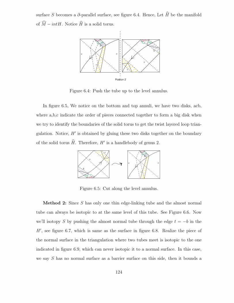
surface S becomes a ∂-parallel surface, see figure 6.4. Hence, Let H be the manifold

of M − intH . Notice H is a solid torus.

Position 2

e

ee

aa

b

b

c

c

Figure 6.4: Push the tube up to the level annulus.

In figure 6.5, We notice on the bottom and top annuli, we have two disks, acb,

where a,b,c indicate the order of pieces connected together to form a big disk when

we try to identify the boundaries of the solid torus to get the twist layered loop trian-

gulation. Notice, H ′ is obtained by gluing these two disks together on the boundary

of the solid torus H. Therefore, H ′ is a handlebody of genus 2.

e

ee

a

a

b

b

c

c

Figure 6.5: Cut along the level annulus.

Method 2: Since S has only one thin edge-linking tube and the almost normal

tube can always be isotopic to at the same level of this tube. See Figure 6.6. Now

we’ll isotopy S by pushing the almost normal tube through the edge t = −b in the

H ′, see figure 6.7, which is same as the surface in figure 6.8. Realize the piece of

the normal surface in the triangulation where two tubes meet is isotopic to the one

indicated in figure 6.9, which can never isotopic it to a normal surface. In this case,

we say S has no normal surface as a barrier surface on this side, then it bounds a

124

handlebody (c.f.[12]). Therefore, we proved that H ′ is a handlebody.

Therefore, S separates M into two genus 2 handlebodies. It is a genus 2 Heegaard

splitting. Since M is not a lens space or S3, then this is a Heegaard splitting with

minimal genus, therefore, it is an irreducible Heegaard splitting.

Now we will show that S is isotopic to the vertical Heegaard splitting surface,

denote it S ′ in the theorem 6.2.

In the Lemma 6.2, we showed that the almost normal tube S ′ can be moved to

along any edge which is not t = −b. Therefore, we can move it to same tetrahedron

where S has two tubes meet together and along the edge e. See figure 6.10. Now we

isotopic S ′ in certain ways shown in figure 6.11, we get the exactly same surface in

figure 6.8inside this triangulation. This shows that this two surface are isotopic to

each other.

add

1 band

push

through

push

through

push

through

e ee

e

fadd

1 band

push

through

Figure 6.6: An almost tube at the same level of the thin edge-linking tube.

After further isotopy the surface in 6.8, we realize that they are all isotopic to

a handlebody S indicated as figure 6.12. It’s not hard to realize that this give us a

genus 2 handlebody (see figure 6.13) in the twisted layered loop triangulation of small

Seifert fibered space M .

Hence, S is isotopic to a vertical Heegaard splitting S ′. Since this is true for any

thin edge-linking tube e, therefore, all the almost normal tubed surface with genus

125

add

1 band

push

through

push

through

push

through

push

through

e ee

adde

1 band

Figure 6.7: Push the almost tube through the edge t = −b.

2, obtained by adding a tube on the a connected normal surface, are isotopic to the

vertical Heegaard splitting S ′.

Theorem 6.4 Any embedded orientable surface in the twisted layered loop triangu-

lation of the small Seifert manifold M is a Heegaard splitting surface, if and only if it

is an almost normal tubed surface such that it is obtained by adding an almost normal

tube on any orientable normal surface with at least one thin edge-linking tube in M .

Proof. =⇒

If S is an embedded orientable Heegaard splitting surface in the twisted layered

loop triangulation of a Seifert manifold M , it is not normal by theorem 6.1. Hence,

S can only be an almost normal surface in M . By theorem 5.2, there is no connected

orientable almost normal octagonal surface. Therefore, S can only be an almost

normal tubed surface.

Since S is a Heegaard splitting, it separates M into two handlebodies H and H ′,

where H is the one that contains the unique vertex in the triangulation. By lemma

6.1, we know that S can not be a surface obtained by adding an almost normal tube

to two disconnected normal surfaces. Hence, it can only be obtained by adding a tube

126

add

1 band

push

through

push

through

e ee

add

1 band

push

through

push

through

e

Figure 6.8: The isotopy of the surface S.

isotopyeeee

Figure 6.9:

to a connected normal surface, denoted by S ′. since S ′ is orientable normal surface,

so S ′ is a vertex-linking S2 possibly with thin edge-linking tubes. Therefore, S is

a vertex-linking S2 with an almost normal tube and possibly with thin edge-linking

tubes. Since M is a small Seifert fibered surface,not a lens space or S3, the Heegaard

splitting surface of it can not have genus 0 or genus 1. Therefore, S should have at

least 2 tubes. Since one of them should be an almost normal tube, S should have at

least one thin edge-linking tube.

⇐=

If S is an almost normal tubed surface obtained by adding an almost normal tube

on any orientable normal surface with at least one thin edge-linking tube in M . By

the Lemma 6.2, we realize that there are 2 possibilities for S in the twisted layered

chain triangulation, an almost normal tubed surface such that the thin edge-linking

127

add

1 band

push

through

push

through

add

1 band

push

through

push

through

eee

e

Figure 6.10: S is the genus 2 handlebody.

tube is around the edge t = −b, and the almost normal tube is along the edge t = −b

and at the same level of the thin edge-linking tube.

By theorem 6.2, If we add the almost tube to the vertex linking 2-sphere with a

thin edge-linking tube around the edge t = −b, it is a Heegaard splitting surface.

For the latter case, S has at least one thin edge-linking tube and the almost normal

tube is along the edge t = −b. Notice this surface always bounds a handlebody on

the side which contains the vertex. Because any vertex-linking S2 with thin edge-

linking tube(s) will bounds a handlebody on the side containing the vertex. If we

add one handle along an edge of the triangulation to this surface, it is still bounds a

handlebody on this side.

Now we need to show that S bounds a handlebody on the other side. Recall that

the almost tube can always be put at the same level with a thin edge-linking tube

around edge e 6= t. If we isotopy S by pushing the almost tube through the edge

t = −b in the direction away from the vertex, we realize that the piece of surface

(figure 6.9) inside this tetrahedron can not be normalized later. Therefore, S has no

normal surface as a barrier surface in this direction. It means it bounds a handlebody.

Therefore, S bounds a handlebody on both sides, so it is a Heegaard splitting

128

add

1 band

push

through

push

through

add

1 band

push

through

push

through

Figure 6.11: The isotopy surface of S.

add

1 band

push

throughpush

through

add

1 band

push

through

push

through

ee e e

e e

1

2

1

2

n+2

Figure 6.12: The isotopy surface of S.

surface of M .

According to this theorem 6.4, theorem 6.2 and 6.3 we can directly get the follow-

ing conclusion.

Theorem 6.5 (Isotopy theorem) There is a unique irreducible Heegaard splitting in

the twisted layered loop triangulation of Seifert fibered space M =Mk = S3/Q4k =

S2((2, 1), (2, 1)(k, 1− k)), up to isotopy. Furthermore, it is a vertical Heegaard split-

129

1

2

3 n+2 1

2

Figure 6.13: The isotopy surface of S.

ting.

Proof. From the theorem 3.1, we know there is no orientable incompressible surface

in Mk, therefore, Mk is a small Seifert fibered manifold, which is non-Haken. Because

any triangulation can catch each strongly irreducible Heegaard splitting class up to

isotopy. In the non-Haken manifold, every irreducible Heegaard splitting surface is

strongly irreducible. All the strongly irreducible Heegaard splittings will be isotopic

to an almost normal surface. Since there is no octagonal almost normal surface in

the twisted layered loop triangulation of Mk, all the irreducible Heegaard splitting

surface are almost normal tubed surfaces.

We showed that all the Heegaard splitting surfaces of genus 2 in M are almost

normal tubed surfaces which obtained by adding an almost normal tube to a vertex-

linking S2 with a thin edge-linking tube in theorem 6.4.

We also showed in theorem 6.3that they are all isotopic to the vertical Heegaard

splitting surface, S, discussed in theorem 6.2.

Therefore, all the genus 2 almost normal surfaces which are Heegaard splitting

surfaces are isotopic to a vertical Heegaard splitting S. And there is no other Heegaard

splittings with less genus than S. Therefore, S is irreducible (c.f.[30]). Therefore,

there is a unique irreducible Heegaard splitting surface of genus 2 in M .

130

6.2 Heegaard splitting surfaces in the layered chain pairs triangulations

In this section, we will study more about the surfaces in the layered chain pair trian-

gulations of Seifert fibered spaces Mr,s=(S2 : (2,−1), (r + 1, 1), (s + 1, 1)), and try to

tell which surface is a Heegaard splitting surface.

6.2.1 Almost normal octaognal Heegaard splitting surfaces

Theorem 6.6 The orientable almost normal octagonal surfaces with genus 2 in the

layered chain pair triangulation of the Seifert fibred spaces M4,3 = M3,4 and M2,6 =

M6,2 are irreducible Heegaard splitting surfaces.

Proof. According to theorem 5.3, there are two almost normal octagonal surfaces with

genus 2 in M4,3 = M3,4 and M2,6 = M6,2, respectively.

1 .The almost octagonal surfaces S and S ′ of genus 2 in C4,3 (or C3,4), with an

edge-weights matching equation of ∂Sr and ∂Ss, 2× (1, 1, 2, 1); 2× (1, 1, 1, 2) ↔

2 × (1, 1, 2, 1); 2 × (1, 1, 1, 2). Here Sr is an octagonal annulus and Ss is two

copies of meridian disks. Notice S is an octagonal surface of genus two. See

figure 5.4. In fact, they are homeomorphic to each other.

On one hand, we can isotopy S and S ′ towards the vertex, and from the figure

6.14, and figure 6.15, we can tell the S is isotopic to a normal surface with

two thin edge-linking tubes, which bounds a handlebody of genus 2 on the side

containing the vertex. On the other hand, we isotopy S and s′ away from the

vertex, and from figure 6.16, it’s not hard to check that S can not fall on any

normal surface. By the barrier theory in the paper [12], S bounds a handlebody

on the side away from vertex. It can be a fun exercise to further isotopy it and

see how it finally looks like a genus two handlebody in C4,3 (or C3,4. Therefore,

S and S ′ are genus two Heegaard splitting surfaces in C4,3 (or C3,4).

131

oct

(1)

push

throughpush

through

push

throughpush

through

oct

(1)

push

throughpush

through

push

throughpush

through

Figure 6.14: Isotopy one possible S towards the vertex.

2 . Two almost normal octagonal surfaces S, S ′ of genus 2 in C6,2 (or C2,6),

with an edge-matching equation of ∂Sr and ∂Ss, 2× (1, 1, 3, 2); 2× (1, 1, 2, 3) ↔

2 × (1, 1, 2, 1) + 2 × (1, 1, 1, 0); 2 × (1, 1, 1, 2) + 2 × (1, 1, 0, 1). Here Sr is an

octagonal annulus and Ss is two copies of meridian disks, (1, 1, 2, 1); (1, 1, 0, 1)

and (1, 1, 1, 0); (1, 1, 1, 2) then the genus of S is 2. See figure 5.5. In fact, they

are homeomorphic to each other.

In these case, we can try to isotopy S, S ′ to both side. See figure 6.17.S can not

isotopy to any normal surface. By the barrier theory in the paper [12], S bounds

a handlebody on each side. Therefore, S is a genus two Heegaard splitting

surface in C6,2 (or C2,6). Since the Heegaard genus of these two manifolds are

2, so these octagonal surfaces are irreducible Heegaard splittings.

132

pushadd

1 band through

push

through

push

through

push

through

(2)

pushadd

1 band throughpush

through

push

throughpush

through

(2)

Figure 6.15: Isotopy S ′ towards the vertex.

Corollary 6.1 The normal surface in the layered chain pair triangulation C4,3 (or

C3,4) that is isotopic to an octagonal almost normal surface is a genus two irreducible

Heegaard splitting.

Proof. Since two almost octagonal surfaces S of genus 2 in C4,3 (or C3,4) are isotopic

to two normal surfaces, repectively. See figure 5.4. Furthermore, these two octagonal

surfaces are Heegaard splitting surfaces. So does these two normal surfaces.

Remark: These two normal Heegaard splitting surfaces in C4,3 are a vertex-

linking S2 with thin edge-linking tubes around edge f3 and edge e3, and a vertex-

linking S2 with thin edge-linking tubes around edge f4 and edge e3, respectively. see

figure 6.14 and 6.15.

Theorem 6.7 Any genus 2 octagonal almost normal surface is isotopic to a normal

133

oct

(1)

pushadd

1 band through

push

through

push

through

push

through

push

throughpush

through

push

throughpush

through

(2)

Figure 6.16: Isotopy S away from the vertex.

surface in Cr,s, r, s ≥ 1, except for the ones in C2,6. Furthermore, each genus 2

octagonal almost normal surface isotopes to a normal surface if we isotopic it in the

direction away from the vertex in Cr,s, r, s ≥ 2, except for the ones in C3,4 and C2,6.

Furthermore, the genus 2 octagonal almost normal surfaces in C3,5 and C2,7 are not

Heegaard splitting surfaces.

Proof. By the corollary 5.1, we notice genus 2 octagonal almost surface only exist in

case 1 and case 2 of the corollary.

1. In Cn,3 = C3,n, n ≥ 5, there are only one almost normal octagonal surfaces of

genus 2.

It has edge-weight matching equation 2 × (1, 1, 2, 1); 2 × (1, 1, 1, 2) ↔ 2 ×

(1, 1, 2, 1); 2× (1, 1, 1, 2).

Notice here Sr is an annulus with no tubes. Therefore, we realize all the pieces

134

(1)

push

throughpush

throughpush

oct

(1)

push

throughpush

throughpush

throughadd

1 band

octpush

through

push

through

push

through

Figure 6.17: Isotopy S towards/away from the vertex.

in the layered chain triangulation in Cr are vertex-linking disks except for the

remaining 4 tetrahedra at the beginning and end of layered chain triangulation

which were restricted by the edge-weights of the annulus Sr. See figure 6.18.

push

through

push

through

push

through

push

through

(2)

push

throughpush

through

Figure 6.18: A genus 2 octagonal almost normal surface in Cn,3.

2. In Cr,2 = C2,r, r ≥ 7, there are only one almost normal octagonal surface of

genus 2.

It has edge-weight matching equation 2 × (1, 1, 3, 2); 2 × (1, 1, 2, 3) ↔ 2 ×

135

(2, 2, 3, 1); 2 × (2, 2, 1, 3) i.e. 2 × (1, 1, 3, 2); 2 × (1, 1, 2, 3) ↔ 2 × (1, 1, 2, 1) +

2 × (1, 1, 1, 0); 2× (1, 1, 1, 2) + 2 × (1, 1, 0, 1).

Notice here Sr is an annulus with no tubes. Therefore, we realize all the pieces

in the layered chain triangulation in Cr are vertex-linking disks except for the

remaining 6 tetrahedra at the beginning and end of layered chain triangulation

which were restricted by the edge-weights of the annulus Sr. See figure 6.19.

add

1 band

push

through

push

throughpush

through

push

through

push

throughpush

throughpush

through

Figure 6.19: A genus 2 octagonal almost normal surface in Cn,2.

We already shows that genus two octagonal surfaces in C4,3 = C3,4 and C2,6 = C6,2

are not isotopic to a normal surface if we push them outwards the vertex. This is how

we prove that they are Heegaard splitting surfaces. However, In C4,3 = C3,4, each

octagonal surface is isotopic to a normal surface when we push it towards the vertex.

Therefore, Only the genus 2 almost normal octagonal surfaces in C2,6 is not isotopic

to a normal surfaces.

Now let’s consider the case in Cn,3 = C3,n, n ≥ 5.

First, consider the case in C5,3. The genus 2 octagonal almost normal surface will

isotopic to a normal surface indicated in figure 6.20.

Notice the normal surface of genus 2 is double cover of a genus 3 nonorientable

surface. Hence, it bounds a twist I boundle of a nonorientable surface, which is not

a handlebody. Therefore, the genus 2 Octagonal almost normal surface in C5,3 is not

a Heegaard splitting surface.

136

push

throughpush

through

(1)

push

through

push

through

add

1 band

push

through

push

throughpush

through

(1)

push

through

push

through

add

2 bands

push

through

Figure 6.20: The barrier normal surface in C5,3.

We can use the same reason to prove that the genus 2 octagonal almost normal

surface in C7,2 is not a Heegaard splitting surface. It is also isotopic to the double

cover of a nonorientable surface. See figure 6.21

It’s not hard to discuss the case in Cn,3,n ≥ 6, and Cn,2, n ≥ 8. They are all

isotopic to a normal surface. See figure 6.22 and 6.23

Open question: From Theorem 6.7, we have a good reason to expect that genus

2 octagonal almost normal surfaces in C2,n, n ≥ 8 and Cn,3, n ≥ 6, are not Heegaard

splitting surfaces. Notice they are all isotopic to a normal surface of genus 2 in

Cr,s with edge-weight matching equation either 2 × (1, 1, 2, 1); 2 × (1, 1, 1, 2) ↔ 2 ×

(1, 1, 2, 1); 2×(1, 1, 1, 2) or 2×(1, 1, 3, 2); 2×(1, 1, 2, 3) ↔ 2×(2, 2, 3, 1); 2×(2, 2, 1, 3).

137

push

through

push

through

push

through

push

through

push

throughadd

1 band

push

through

push

through

push

through

push

through

push

through

push

through

push

through

add

2 bands

Figure 6.21: The barrier normal surface in C5,3.

6.2.2 Almost normal tubed Heegaard splitting surfaces

Now we will consider the almost normal tubed surfaces in the layered chain pair

triangulation of Mr,s. We will give the classification of the irreducible Heegaard

splitting.

According to the theorem 4.2, there are three types of orientable normal surfaces

in Cr,s.

1. a vertex-linking S2 (possibly) with thin edge-linking tubes, denoted by type I

surface.

2. a surface of genus n, n ≥ 2, which has non thin edge-linking tubes, denoted by

type II normal surfaces.

They have edge-weights matching equations either 2×(1, 1, 2, 1); 2×(1, 1, 1, 2) ↔

2× (1, 1, 2, 1); 2× (1, 1, 1, 2) or 2× (1, 1, 3, 2); 2× (1, 1, 2, 3) ↔ 2× (2, 2, 3, 1); 2×

(2, 2, 1, 3).

138

3. a nonseparating torus, which only exist in C3,3 and C5,2 = C2,5. They have edge-

weights matching equation 2 × (1, 1, 2, 1); 2 × (1, 1, 1, 2) ↔ 2 × (1, 1, 2, 1); 2 ×

(1, 1, 1, 2), 2 × (1, 1, 3, 2); 2× (1, 1, 2, 3) ↔ 2 × (2, 2, 3, 1); 2× (2, 2, 1, 3), respec-

tively.

Now let’s consider what kind of surfaces we will get if we add an almost normal tube

to a connected orientable normal surface.

Theorem 6.8 If we add an almost normal tube along an edge to a nonseparating

torus in C3,3 and C2,5, we will get a nonorientable surface.

Proof. The only way to add the almost normal tube to the nonseparating torus in C3,3,

up to isotopy, are shown in figure 6.24. It is isotpoic to a genus 2 nonorientable surface,

with edge-weight matching equation (1, 1, 0, 1); (1, 1, 1, 0) ↔ (1, 1, 0, 1); (1, 1, 1, 0).

The same method can also applied to the nonseparating torus in C2,5. It is

isotopic to a genus 2 nonorientable surface, with edge-weight matching equation

(1, 1, 1, 0); (1, 1, 0, 1) ↔ (0, 0, 1, 1); (0, 0, 1, 1).

See figure 6.25.

According to the theorem 4.2, every normal surface with genus 1 is either vertex-

linking 2-sphere with one thin edge-linking tube in any Cr,s, r, s ≥ 2 or a nonseparat-

ing torus in C3,3 or C5,2. In the theorem 6.8, we just showed that if we add an almost

normal tube to a nonseparating torus in C3,3 or C5,2, we will get a nonorientable sur-

face.If we attached the almost normal tube to other orientable normal surface from

type II, which has a non thin-edge linking tube, then it is a surface with genus at

least 3. It is also not hard to show that these surfaces are also Heegaard splitting

surfaces.

Let S be a vertex-linking 2-sphere with a thin edge-linking tube. If the almost

normal tube is attached along an edge which doesn’t intersect with any quads of

139

S, it will normally isotopic to a vertex-linking 2-sphere with two thin edge-linking

tubes. From the discussion of last section, we know some of this type of surfaces

are Heegaard splitting surfaces and some of them are not. From now on we only

consider the surface which is a vertex-linking 2-sphere with 2 tubes such that the

almost normal tube is at the same level of the thin edge-linking tube.

Theorem 6.9 Let S be an orientable genus 2 almost normal tubed surface with an

almost normal tube at the same level of a thin edge-linking tube in Mr,s, r, s ≥ 2, then

it is a Heegaard splitting surface. Furthermore, they are isotopic to each other and

are all vertical Heegaard splitting surfaces.

Proof. Since S is an orientable genus 2 almost normal tubed surface with an almost

normal tube at the same level of an thin edge-linking tube. For convenience, we use

Si to denote this type of surface and with one thin edge-lining tube around the edge

i in Cr,s. The complete list of all these Si is Sf1 = Sfr+2 = Se1 = Ses+2 , Sτ = Se2,

Sβ = Ses+1, St = Sf2 , Sb = Sfk+1and Se, e is any other edge in Cr,s. Now we want to

show these surfaces are the same, up to isotopy.

For surface Se, if the edge e is in Cr, and e is any edge except for τ = −e2,

β = −er+1 and f1 = −fr+2 = −e1 = es+2. Now we will show Se is isotopy to

Sτ = Se2 . This is indicated in figure 6.26. Se is on the top of the figure and Sτ is

on the bottom of the figure. These two surfaces looks exactly the same after isotopy,

when they were pushed away from the vertex.

Let Sβ be a genus 2 almost normal tubed surface with the thin edge-linking tube

around the edge β. Since we can isotopy the almost normal tube on Se to along the

edge β. See figure 6.27. Se is the surface on the top of the figure and can be isotopy

to Sβ on the bottom of the figure.

Therefore, Sτ = Se = Sβ , up to isotopic.

For Sf1 , an orientable genus 2 almost normal tubed surface, it is obtained by

140

adding an almost normal tube to a vertex-linking S2 with one thin edge-linking tube

around f1 = −fk+2 = e1 = −ek+2. See figure 6.28. Sf1 is the surface on the top of

the figure and it can be isotopy to Sτ on the bottom of the figure.

Hence, we have Sf1 = Sτ = Se2, up to the isotopic.

Therefore, we proved Sτ = Sβ=Se, for e is every edge in Cr except for f2 = −t

and fr+1 = b.

Since f1 = −fr+2 = e1 = −es+2, so Se1 and Sf1 is the same surface. Since

Cr,s = Cs,r, up to isomorphisim, if we switch the role of r and s, we can show that

St=Sb=Se, up to isotopy, where e is every edge in Cs, except for e2 = −τ and

es+1 = −β, by using the same figure 6.26, 6.27 and 6.28.

All in all, Sτ=Sβ=t=Sb=Se, e is any other edge in Cr,s, up to isotopy.

Therefore, all the genus two almost normal tubed surface are isotopy.

Furthermore, we notice they are all vertical Heegaard splitting surfaces, Because

they can all be viewed as a boundary surface of a neighborhood of an exceptional fiber

with an arc attach to it, which will be projected to be a loop based on the project

point of this exceptional fibers. Moreover, Sf1 is a verical Heegaard splitting surface

with respective to the exceptional fiber with multiplicity 2, Sτ is a verical Heegaard

splitting surface with respective to the exceptional fiber with multiplicity r + 1, and

St is a verical Heegaard splitting surface with respective to the exceptional fiber with

multiplicity s+1. Notice these are all possible vertical Heegaard splittings in Mr,s, and

they are isotopic to each other, therefore, there is unique vertical Heegaard splitting

surface, up to isotopy, in the layered chain triangulation.

Theorem 6.10 (Isotopy theorem) In a layered chain pair triangulation of Mr,s, r, s ≥

1, there exists a unique vertical Heegaard splitting, up to isotopy.

Proof. Since in any layered chain triangulation of Cr,s, the genus 2 almost tubed

surfaces with an almost normal tube at the same level of an thin edge-linking tube

141

are Heegaard splitting surfaces. Furthermore, we know all these almost normal tubed

surfaces are not only vertical Heegaard splittings, but also includes all three possible

vertical Heegaard splitting surfaces, up to isotopy. We proved that they are isotopic

to each other for s, r ≥ 2 according to theorem 6.9. Hence, there is a unique vertical

Heegaard splitting surface, up to isotopy. If s = 1 or r = 1, by theorem 6.5, there is

only one vertical Heegaard splitting up to isotopy. Therefore, in a layered chain pair

triangulation of Mr, s, r, s ≥ 1, there exists a unqiue vertical Heegaard splitting, up

to isotopy.

Corollary 6.2 There is only one genus 2 irreducible Heegaard splitting surface in

M2,7 and M3,5, up to isotopy.

Proof. Since we know that in small Seifert fiber spaces M2,7 and M3,5, every irreducible

Heegaard splitting surfaces are strongly irreducible. Furthermore, every strongly

irreducible Heegaard splitting surface up to isotopy will be normally isotopy to an

almost normal surface. In these two manifolds, we proved in Theorem 6.7 that genus

2 octagonal surfaces are not Heegaard splitting surfaces. Therefore, all the Heegaard

splitting surfaces of genus 2 can only be almost normal tubed surfaces. By Theorem

6.10, there is only one genus 2 irreducible Heegaard splitting surface up to isotopy.

Here, we finish our discussion of genus 2 irreducible Heegaard splitting surfaces

in Mr,s, r, s ≥ 1. There is some questions that we are still working on. For example,

we hope to give a proof that all the genus two octagonal almost normal surfaces

are not Heegaard splitting surface in Mr,s, except for M3,4 and M2,6. Two octagonal

Heegaard splitting surfaces are very likely to be horizontal Heegaard splitting surfaces

in M3,4 and M2,6, respectively. This may leads to a complete classification of genus

two Heegaard splitting surfaces, up to isotopy.

142

add

1 band

(2)

push

through

push

through

push

throughpush

through

(2)

push

throughpush

through

push

through

add

1 band

push

throughpush

through

push

throughpush

through

push

through

push

throughpush

through

push

through

push

throughpush

through

push

throughpush

through

push

through

add

1 band

push

throughpush

through

add

1 band

push

through

push

through

push

through

push

through

push

throughpush

through

push

throughpush

through

isotopy in Cn,3, n ≥ 6

isotopy in Cn,2, n ≥ 8

Figure 6.22: The barrier normal surface in Cn,3.

143

add

1 band

push

through

push

through

push

throughpush

through

push

through

push

throughpush

through

push

through

add

1 band

push

through

push

through

push

through

push

through

push

throughpush

through

push

throughpush

through

Figure 6.23: The barrier normal surface in Cn,2

.

144

isotopy

isotopy

Figure 6.24:

145

push

throughpush

through

push

through

push

through

push

through

push

throughpush

through

push

through

push

through

push

through

push

througha band

push

through

push

through

add

a band

add

isotopy

isotopy

Figure 6.25:

146

e ee

e

e ee

e

e ee

e

eee e

eee e

isotopy

isotopy

isotopy

isotopy

Figure 6.26:

147

e ee

e

push

through

e ee

e

e ee

e

isotopy

isotopy

isotopy

isotopy

Figure 6.27:

148

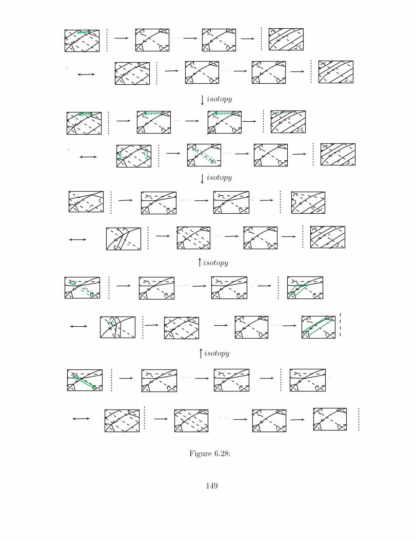
e

e

e

e

e

e

e

e

a

d

c

b

e

isotopy

isotopy

isotopy

isotopy

Figure 6.28:

149

BIBLIOGRAPHY

[1] M. Boileau, D.J. Collins and Zieschang, Genus 2 Heegaard Decompositions of

Small Seifert Manifolds, Ann. Inst. Fourier, Grenoble, 41, 4(1991), 1005-1024.

[2] M. Boileau, J.P. Otal, Groupes des diffe topies de cetaines varietes des Seifert.

C.R. Acad. Sci. Paris, 303-I (1986), 19-22.

[3] F. Bonahon and J.P. Otal, Scindements de Heegaard des espaces lenticulaires,

Ann. Sci. Ec. Norm. Sup, 16 (1983), 451-466.

[4] Benjamin Burton, Minimal triangulations and normal surfaces, PhD Thesis,

University of Melbourne, 2003.

[5] A. J. Casson and C. McA. Gordon. Reducing Heegaard splittings. Topology

and its Applications.27:275-283, 1987.

[6] Huai-Dong Cao and Xi-Ping Zhu, A complete proof of the Poincare and

geometrization conjectures-application of the Hamilton-Perelman theory of

the Ricci flow, Asian J. Math. 10 (2006), no. 2, 165-492, Erratum, p. 663.

MR2233789.

[7] W. Haken, Theorie der normalflachen, Acta Math. 105 (1961), 245-375. MR

25:4519a.

[8] Allen Hatcher, Notes on basic 3-manifold topology, on his webpage.

[9] Poul Heegaard, Forstudier til en topologiskteori for de alebraiske fladers sam-

menhaeng. Ph.D. thesis, 1898.

150

[10] J. Hempel, 3-manifolds, Princeton University Press, 1976. MR 54:3702.

[11] William Jaco, Lectures on Three-Manifold Topology, America Mathematics

Socitey,1980.

[12] William Jaco and J. Hyam Rubinstein, 0-efficient triangulations of 3-manifolds,

J. Differential Geometry, 65(2003),no.1, 61-168.

[13] William Jaco and J. Hyam Rubinstein, Layered-triangulations of 3-manifolds.

Preprint, (2006), j96 pages, math.GT/0603601.

[14] William Jaco and J. Hyam Rubinstein, Inflating ideal triangulations, preprint.

[15] William Jaco, J. Hyam Rubinstein and Stephan Tillmann, Minimal trian-

gulations for an infinite family of lens spaces, Journal of Topology 2 (2009)

157–180.

[16] William Jaco, J. Hyam Rubinstein and Stephan Tillmann, Coverings and Min-

imal triangulations of 3-manifolds, 2009, arXiv:math.

[17] Bruce Kleiner and John Lott, Notes on Perelman’s papers, arXiv:

math/0605667.

[18] John Morgan and Gang Tian, Ricci flow and the Poincare conjecture, Clay

Mathematical Monographs, vol. 3, American Mathematical Society, Provi-

dence, RI, 2007

[19] Yoav Moriah, Heegaard splittings of Seifert fibered spaces, Inventiones math-

ematicae, 91, 465-481, 1988.

[20] Yoav Moriah and Jennifer Schultens, Irreducible Heegaard splittings of Seifert

fibered spaces are either vertical or horizontal, Topology, Vol. 37, No. 5, pp.

1098-1112, 1998.

151

[21] Peter Orlik, Seifert Manifolds, Lecture Notes in Mathematics, no.291,

Springer-Verlag, Berlin, 1972.

[22] Grisha Perelman, The entropy formula for the Ricci flow and its geometric

application.

[23] Grisha Perelman, Finite extinction time for the solutions to the Ricci flow and

its geometric applications.

[24] Grisha Perelman, Ricci flow with surgery on three-manifolds.

[25] J. Hyam Rubinstein, On 3-manifolds that have finite fundamental group and

contain Klein bottles, Trans. Amer. Math. Soc. 251(1979),129-137.

[26] J. Hyam Rubinstein, One-sided heegaard splittings of 3-manifolds, Pacific

Journal of Mathematics, Vol. 76, No. 1, 1978.

[27] J. Hyam Rubinstein, Polyhedral minimal surfaces, Heegaard splittings and

decision problems for 3-dimensional manifolds, Proceedings of the Georgia

Topology Conference, AMS/IP Stud. Adv. Math., vol. 21, Amer. Math. Soc.,

Providence, RI, 1997, pp. 1-20. MR 98f:57030.

[28] Martin Scharlemann, Heegaard splittings of Compact 3-Manifolds, Handbook

of geometric topology, edited by R.J. Daverman and R.B. Sher, 923-951.

[29] Jennifer Schultens, Weakly reducible Heegaard splittings of Seifert fibered

spaces, preprint.

[30] Eric Sedgwick,The irreducibility of Heegaard splittings of Seifert fibered

spaces, Pacific Journal of Mathematics, Vol. 190, No. 1, 1999.

[31] H.Seifert and W. Threlfall, A Textbook of topology, and Seifert: Topology of

3-dimensional fibered spaces.

152

[32] P. Scott, The eight geometries of 3-manifolds, Bulletin of London Mathematics

Society, 1993,67(3),425-448.

[33] F. Waldhausen, Heegaard-Zerlegungen der 3-Sphare, Topology 7(1968), 195-

203.

153

VITA

Zhenyi Liu

Candidate for the Degree of

Doctor of Philosophy

Dissertation: TRIANGULATIONS AND HEEGAARD SPLITTINGS

Major Field: Mathematics

Biographical:

Personal Data: Born in Yantai, Shandong, China on March 30, 1979.

Education:Received the B.S. degree from Yantai Teachers’ University, Yantai, Shan-dong, China, 1997 - 2000, in Mathematics and Applied Mathematics.Received the M.S. degree from Southwest Jiaotong University, Chengdu,Sichuan, China, 2000 - 2003, in Applied Mathematics.Completed the requirements for the degree of Doctor of Philosophy with amajor in Pure Mathematics at Oklahoma State University in May, 2010.

Experience:Teaching Assistant, in the Math department, at Oklahoma State Univer-sity, 2003 - 2010.

Name: ZHENYI LIU Date of Degree: May, 2010

Institution: Oklahoma State University Location: Stillwater, Oklahoma

Title of Study: TRIANGULATIONS AND HEEGAARD SPLITTINGS

Pages in Study: 153 Candidate for the Degree of Doctor of Philosophy

Major Field: Mathematics

Recently William Jaco, J. Hyam Rubinstein and Stephan Tillmann together provedthat the generalized quaternion spaces S3/Q4k, k ≥ 2, which are small Seifert fiberedspaces Mk= (S2 : (2, 1), (2, 1), (k,−k + 1)), have complexity k, which is the minimalnumber of tetrahedra in a triangulation of Mk. The techniques used can be expandedto show that the layered chain pair triangulations of Seifert fibered spaces (S2 :(2,−1), (r + 1, 1), (s + 1, 1)), r, s ≥ 1 are minimal.

My thesis is to closely study the minimal, 0-efficient triangulations of the above twoinfinite families of Seifert fiberd spaces. One family is called the twisted layered looptriangulation, and the other family is called layered chain pair triangulations. Theywere named by Ben Burton. We classify all normal and almost normal surfaces byidentifying one-sided incompressible surfaces, orientable incompressible surfaces andHeegaard splitting surfaces. We also use combinatorial methods to study and classifyirreducible Heegaard splitting surfaces, up to isotopy, in these two infinite families ofSeifert fibered manifolds.

In the twisted layered loop triangulations of the Seifert fibered space Mk, k ≥ 2. Weprove that a properly embedded surface S is a Heegaard splitting surface if and onlyif it is an almost normal tubed surface with the almost normal tube at the same levelof a thin edge-linking tube. Furthermore, any genus two Heegaard splitting surfaceis vertical. A combinatorial proof is given that there is a unique irreducible genus 2Heegaard splitting surface, up to isotopy, in Mk, k ≥ 2.

In the layered chain pair triangulation of Seifert fibered spaces Mr,s=(S2 : (2,−1), (r+1, 1), (s+1, 1)), r, s ≥ 1, we prove that an almost normal tubed surface with the almostnormal tube at the same level of a thin edge-linking tube is a Heegaard splittingsurface. Moreover, if the genus of it is 2, then it is not only an irreducible Heegaardsplitting but also a vertical one. We give a combinatorial proof that there is a uniqueirreducible vertical Heegaard splitting surface, up to isotopy, in Mr,s, r, s ≥ 1.

Our work follows the methods used by Jaco and Rubinstein in studying layered-triangulations of the solid torus and their classification of normal surfaces in thesetriangulations.

ADVISOR’S APPROVAL: